Curved geometries from planar director fields -
Solving the two-dimensional inverse problem

Abstract

Thin nematic elastomers, composite hydrogels and plant tissues are among many systems that display uniform anisotropic deformation upon external actuation. In these materials, the spatial orientation variation of a local director field induces intricate global shape changes. Despite extensive recent efforts, to date, there is no general solution to the inverse design problem: how to design a director field that deforms exactly into a desired surface geometry upon actuation, or whether such a field exists. In this work, we phrase this inverse problem as a hyperbolic system of differential equations. We prove that the inverse problem is locally integrable, provide an algorithm for its integration, and derive bounds on global solutions. We classify the set of director fields that deform into a given surface, thus paving the way to finding optimized fields.

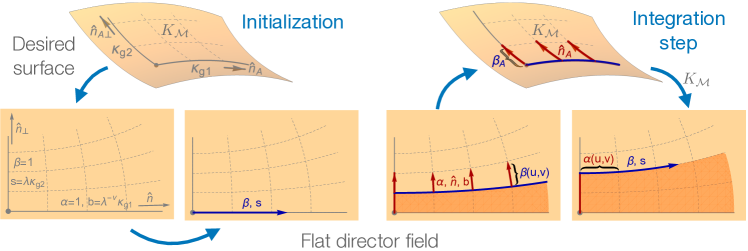
Figure 1: Integration of the director field. Left: Initialization. Given a surface with curvature $K$ the initial condition consists of two perpendicular curves that will become integral curves of the actuated director and its perpendicular. The corresponding unactuated integral curves inherit the geosedic curvatures $b=\lambda^{-\nu}\kappa_{g1}$ and $s=\lambda\kappa_{g2}$ respectively, and we are free to set $\alpha=1$ along the former and $\beta=1$ along the latter. We next integrate to obtain $\beta$ and $s$ along the director integral curve completing the initialization of the SOE. Right: Iterative integration step. (i) $\alpha,\hat{\mathbf{n}},\mathbf{r}$ and $b$ are integrated a $dv$ step along $\hat{\mathbf{n}}_{\perp}$ on the flat sheet. $\hat{\mathbf{n}}_{\!A}$ and $\mathbf{r}_{\!A}$ are integrated a step $dv$ along $\hat{\mathbf{n}}_{A\perp}$ on the desired curved surface. (ii) $\beta$ and $s$ are integrated along $\hat{\mathbf{n}}$ according to the Gaussian curvature $K_{\mathcal{M}}$ pulled back from the desired surface. With the information at hand this step can now be reiterated.

Many fiber-reinforced thin biological tissues Fahn and Zohary (1955); Armon et al. (2011); Reyssat and Mahadevan (2009); Aharoni et al. (2012) and synthetic sheets of responsive materials Sydney Gladman et al. (2016); Mostajeran et al. (2016); Aharoni et al. (2018); Warner and Mostajeran (2018); Kowalski et al. (2018) deform into their desired shapes by a uniform anisotropic deformation. Upon actuation these effectively 2D materials expand by a constant factor along the fibers and shrink by a different factor along the perpendicular direction. While the length variations along these principal axes are constant across the material, the spatial variation in the direction of the principal axes allows this simple mode of uniform deformation to result in rich and intricate shapes.

The fiber orientation is described by the field $\hat{\mathbf{n}}(\mathbf{r})$ called the director. Together with the spatially constant shrinkage/expansion factors the director field uniquely defines the two-dimensional geometry that is obtained upon actuation. The actuation can be achieved through changing a variety of ambient conditions: temperature or light in liquid crystal elastomers Küpfer and Finkelmann (1991); Finkelmann et al. (2001); Warner and Terentjev (2003), humidity for a variety of plants Fahn and Zohary (1955); Armon et al. (2011); Reyssat and Mahadevan (2009), and immersion in water in fiber-reinforces hydrogels Sydney Gladman et al. (2016).

Predicting the geometry obtained upon activation as a function of the prescribed director field has been recently resolved Modes et al. (2010); Modes and Warner (2011); Aharoni et al. (2014); Mostajeran (2015). This geometry, captured by the two dimensional Riemannian metric, however, does not uniquely define the obtained surface. A given metric will correspond to a wide and typically continuous family of surfaces. The geometric rigidity that arises from Gaussian curvature sign variations as well as imposed boundary conditions serve to narrow down this wide family. Nonetheless, selecting the desired surface among all embeddings requires some control over the principal curvatures of the surface. Several techniques to partially control the principal curvatures of the thin sheet have been proposed and implemented Aharoni et al. (2014); Sydney Gladman et al. (2016); Aharoni et al. (2018), yet these techniques are system-specific and depend strongly on the elastic constitutive relations. In what follows we only address the universal problem associated with controlling the two-dimensional Riemannian geometry. The desired surface is an isometric embedding of the obtained solution, however, other embeddings may exist. Selecting among these will be addressed in the future.

Recent responsive 3D printing (often termed 4D) applications Sydney Gladman et al. (2016) and advances in programmable nematic elastomer production Aharoni et al. (2018) are aimed at producing a desired surface upon actuation, and thus give rise to the inverse problem: What is the planar director orientation field that will result in a desired geometry upon actuation? There have been several recent advances in addressing the inverse problem. In Aharoni et al. (2014); Warner and Mostajeran (2018); Kowalski et al. (2018) director fields are found for surfaces of revolution while in Aharoni et al. (2018) approximate solutions are found numerically for arbitrary surface geometries. In Plucinsky et al. (2016); Siéfert et al. (2019) the anisotropic deformation was allowed to vary spatially, leading to a less constrained inverse problem, to which possible solutions were presented. Alas, an exact solution to the full inverse problem was not found in the general case, nor was it shown to exist.

In this letter we formulate the inverse problem as a set of partial differential equations (PDEs). We show that the system is well posed and demonstrate director fields that curve into arbitrary surfaces by integrating these equations. We present an algorithm that when provided with a desired geometry and appropriate initial conditions integrates the sought director field. This approach allows us to explore the limits of director induced deformations and characterize the set of director fields that produce a desired geometry. Characterizing the collection of solutions opens the door to optimization of the choice of initial data with respect to desirable properties such as maximizing coverage or minimizing distortions.

To find the set of equations describing the inverse problem, we first rephrase the recently solved forward problem: What is the geometry assumed when a prescribed director field is actuated.

The forward problem. — Consider an initially flat thin sheet made of a uniform material characterized by a planar director field $\hat{\mathbf{n}}=(\cos(\theta),\sin(\theta))$. Upon actuation the material shrinks by a factor $\lambda$ along the director and expands by a factor $\lambda^{-\nu}$ along the perpendicular direction. As shown in Aharoni et al. (2014); Mostajeran (2015) the Gaussian curvature of the actuated surface reads

$$K_{\!A}=(\lambda^{2\nu}-\lambda^{-2})\times\Bigl{(} \cos(2\theta)\left((\partial_{y}\theta)^{2}-(\partial_{x}\theta)^{2}+\partial_{x}\partial_{y}\theta\right)$$

$$+\frac{\sin(2\theta)}{2}\left(\partial_{x}^{2}\theta-4\partial_{x}\theta\partial_{y}\theta-\partial_{y}^{2}\theta\right)\Bigr{)}.$$

Solving the inverse problem amounts to finding a planar director field, $\theta(x,y)$, that satisfies the above non-linear partial differential equation. This formidable problem is further complicated as the Gaussian curvature is naturally given on the curved surface, and not in the Cartesian coordinates $(x,y)$.

Exploiting the natural coordinates and scalars that characterize the director field Niv and Efrati (2018) we next recast the system in a form that allows explicit integration of the inverse problem. In two-dimensions one may always define a parametrization $\mathbf{r}(u,v)$ such that $u$ parametric curves (along which $v$ is constant) are everywhere tangent to the director, whereas the $v$ parametric lines are perpendicular to the director,

$$\partial_{u}\mathbf{r}=\alpha\hat{\mathbf{n}},\qquad\partial_{v}\mathbf{r}=\beta\hat{\mathbf{n}}_{\perp}.$$ (1)

The metric of the flat sheet with respect to this parametrization is given by $dl^{2}=\alpha^{2}du^{2}+\beta^{2}dv^{2}$. Upon actuation the flat sheet shrinks and expands along $\hat{\mathbf{n}}$ and $\hat{\mathbf{n}}_{\perp}$ respectively. The arc-length parameters thus change according to

$$\alpha_{\!A}=\lambda\alpha,\qquad\beta_{\!A}=\lambda^{-\nu}\beta,$$ (2)

and the actuated metric remains diagonal and is given by $dl_{\!A}^{2}=\alpha_{\!A}^{2}du^{2}+\beta_{\!A}^{2}dv^{2}$.

A two dimensional director field, $\hat{\mathbf{n}}$, is fully characterized by two local scalar fields Niv and Efrati (2018); its intrinsic bend, $b$, and splay, $s$, which are given by

$$b=\hat{\mathbf{n}}_{\perp}\cdot(\hat{\mathbf{n}}\cdot\nabla)\hat{\mathbf{n}}\,,\qquad s=\hat{\mathbf{n}}_{\perp}\cdot(\hat{\mathbf{n}}_{\perp}\cdot\nabla)\hat{\mathbf{n}}\,.$$ (3)

Geometrically, the bend and splay represent gradients in $\hat{\mathbf{n}}$ along $\hat{\mathbf{n}}$ and across it, and correspond to the geodesic curvatures of the $u$ and $v$ parametric curves, respectively. They are thus related to the flat arc-lengths by

$$b=-\frac{\partial_{v}\alpha}{\alpha\beta},\qquad s=\frac{\partial_{u}\beta}{\alpha\beta}.$$ (4)

Given the two dimensional metric one could express the Gaussian curvature in terms of the splay, the bend and their directional derivatives. For the case where the director is given in a planar domain this leads to

$$0=s^{2}+\frac{1}{\alpha}\partial_{u}s+b^{2}-\frac{1}{\beta}\partial_{v}b,$$ (5)

see Niv and Efrati (2018); SM . Upon actuation the metric component rescale according to (2) and the actuated Gaussian curvature reads

$$-K_{\!A}=\lambda^{-2}\left(s^{2}+\frac{1}{\alpha}\partial_{u}s\right)+\lambda^{2\nu}\left(b^{2}-\frac{1}{\beta}\partial_{v}b\right).$$ (6)

As the actuated geometry is fully described by $K_{\!A}$ this completes the solution of the forward problem.

The inverse problem. — Given a curved surface $\mathcal{M}$ with Gaussian curvature $K_{\mathcal{M}}$, we seek a flat director field $\hat{\mathbf{n}}$ that upon actuation will assume the geometry of $\mathcal{M}$, and in particular $K_{\!A}=K_{\mathcal{M}}$.

Combining equations (5) and (6) we find the propagation equations for the bend $b$ and splay $s$ on the flat sheet along $\hat{\mathbf{n}}_{\perp}$ and $\hat{\mathbf{n}}$

$$\frac{1}{\beta}\partial_{v}b =b^{2}-\frac{K_{\mathcal{M}}}{\lambda^{-2}-\lambda^{2\nu}},$$ (7)

$$\frac{1}{\alpha}\partial_{u}s =-s^{2}-\frac{K_{\mathcal{M}}}{\lambda^{-2}-\lambda^{2\nu}}.$$

The System Of Equations (SOE) comprised of (1),(3),(4) and (7) allows us to find a parametrization of a flat sheet, $\mathbf{r}(u,v)$, and a director field tangent to the $u$-parametric curves $\hat{\mathbf{n}}\propto\partial_{u}\mathbf{r}$, such that when the flat sheet is actuated it deforms into a surface with the desired curvature $K_{\mathcal{M}}$.

Not all systems of partial differential equations are solvable. To allow a solution from initial data they must satisfy integrability conditions. These estimate the predicted variation of the solution along closed paths, and must vanish. The integrability conditions for Eq.(1), which propagate $\mathbf{r}$, are synonymous with equations (3) and (4). The integrability conditions for (3), which propagate $\hat{\mathbf{n}}$, yield (5). The remaining differential relations, namely (4) and (7), propagate information only along one direction and thus cannot lead to contradictions in the integrated value of the solutions.

In the particular and simple case where the desired geometry is characterized by $K_{\mathcal{M}}=const$, the SOE are self-contained and can be integrated directly. This will result in a planar director field $\hat{\mathbf{n}}$ that when actuated will adopt the geometry of constant Gaussian curvature $K_{\mathcal{M}}$, as can be seen in Fig. 2 and 3.

In contrast, when the desired geometry is characterized by a spatially varying Gaussian curvature the SOE is not self-contained, as solving equations (7) requires knowledge of the curvature $K_{\mathcal{M}}(u,v)$ at position $\mathbf{r}_{\!A}$. This, in turn, requires that we also know the embedding $\mathbf{r}_{\!A}(u,v)$. While $\alpha_{\!A},\beta_{\!A},b_{\!A}$ and $s_{\!A}$ are algebraically related to their flat counterparts, through equations (2) and (4), this does not hold for the actuated director field $\hat{\mathbf{n}}_{\!A}$ and the exact embedding $\mathbf{r}_{\!A}(u,v)$. To obtain the director $\hat{\mathbf{n}}_{\!A}$ and embedding $\mathbf{r}_{\!A}(u,v)$ one has to integrate the curved versions of equations (3) and (1) respectively.

This results in an integration scheme in which at every step one solves $\alpha,\beta,b,s,\hat{\mathbf{n}}$ and $\mathbf{r}(u,v)$ on the flat sheet, and then uses this information to integrate $\hat{\mathbf{n}}_{\!A}$ and $\mathbf{r}_{\!A}$ to obtain $K_{\mathcal{M}}(u,v)$ for the next integration step, as depicted in Fig. 1. See Supplemental Material (SM) for more details SM .

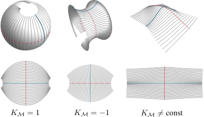
Figure 2: Solutions of the SOE: Director curves on a flat sheet and the shapes they take when actuated, found by integrating the SOE. Left: Sphere with Gaussian curvature $K_{\mathcal{M}}=1$. Center: Constant negative-curvature, $K_{\mathcal{M}}=-1$, body of rotation. Right: Anisotropic Gaussian surface, with varying Gaussian curvature.

Initial conditions. — Given a curved surface $\mathcal{M}$, solving the inverse problem amounts to finding a director field $\hat{\mathbf{n}}$ that satisfies the SOE with respect to $\mathcal{M}$ in a flat domain $\mathcal{D}$.

To solve the Cauchy problem for the SOE, i.e. to find initial conditions around which unique solutions exist, and to characterize these solutions we first need to understand the structure of the SOE. Equations (5) and (6) form a hyperbolic set of equations for $s$ and $b$. Bringing them to their canonical form (7) identifies the characteristic lines along which information propagates with the parametric curves of $u$ and $v$. Examining equations (4) we find a similar hyperbolic structure, and that the role of the parametric curves as carriers of partial information is preserved also for $\alpha$ and $\beta$. Initial data for $\alpha$ and $b$, the arc-length and geodesic curvature of $u$-lines, is propagated along $v$-lines, while initial data for $\beta$ and $s$, the arc-length and geodesic curvature of $v$-lines, propagates along $u$-lines. Once $\alpha,\beta,b$ and $s$ are known, $\hat{\mathbf{n}}$ and $\mathbf{r}$ can be obtained by directly integrating (3) and (1) respectively. The structure of the SOE is quasi-linear and is reminiscent of the equations associated with the embedding of hyperbolic surfaces in $\mathbb{R}^{3}$ Rozhdestvenskii (1962); Poznyak and Shikin (1995).

This hyperbolic structure implies that prescribing $\alpha,\beta,b$ and $s$ along a non-characteristic curve $\gamma\in\mathcal{D}$, as well as $\hat{\mathbf{n}}$ and $\mathbf{r}$ at some point along the curve, leads to a unique solution in its vicinity Hadamard (1923). Equivalent types of initial data that could be used include prescribing $\hat{\mathbf{n}}$ and $\mathbf{\nabla}_{\perp}\hat{\mathbf{n}}$ along $\gamma$, or alternatively prescribing $\hat{\mathbf{n}}$ and $b$ along the same curve.

A particularly convenient and geometrically transparent choice for the system at hand is prescribing a Goursat initial condition Goursat (1923), in which the initial data is divided into two components each given on a different line. Specifically we pick two orthogonal curves in $\mathcal{M}$, one of which we set to be a $u$-line (i.e. an integral curve of the director) and the other a $v$-line (an integral curve of the perpendicular to the director). We next show how to integrate the SOE from such initial conditions.

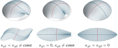
Figure 3: Distinct director fields (bottom) deforming into the same section of the unit sphere (top). The solutions are characterized by the geodesic curvatures of the initial curves, the $u$-base line (thick blue) with $\kappa_{g1}$ and the $v$-base line (dashed red) with $\kappa_{g2}$, from which they are integrated.

Integrating the inverse equation. — The solution is initialized by pulling back the two initial curves on the curved surface $\mathcal{M}$, onto the flat domain $\mathcal{D}$ by integrating equations (1) and (3) (Fig. 1 left). The bend and splay of the flat director field in $\mathcal{D}$ are algebraically related to the actuated bend and splay, which correspond to the geodesic curvature of the $u$-line and $v$-line in $\mathcal{M}$ respectively. The arc-lengths’ gauge freedom is fixed by setting $\alpha$ to $1$ on the $u$-line, and $\beta$ to $1$ on the $v$-line. This completes the setting of the Goursat initial condition – two perpendicular characteristic curves in $\mathcal{D}$, the $u$-baseline along which we know $\alpha$ and $b$, and the $v$-baseline along which $\beta$ and $s$ are known. We finish the initialization step by obtaining the values of $\beta$ and $s$ along the $u$-baseline through the integration of equations (4) and  (7).

Following the initialization, the SOE is integrated via a reiterated two-step tango: Knowing $\mathbf{r},\hat{\mathbf{n}},\mathbf{r}_{\!A},\hat{\mathbf{n}}_{\!A},\alpha,\beta,s,b$ on a $u$-line allows us to integrate $\mathbf{r},\mathbf{r}_{\!A},\hat{\mathbf{n}},\hat{\mathbf{n}}_{\!A},\alpha,b$ one integration step along $v$, creating the next $u$-line. The missing information for $\beta$ and $s$ does not propagate along $v$, but can now be integrated from the $v$-baseline along the newly formed $u$-line. The Gaussian curvature $K_{\mathcal{M}}$ is inherited through the embedding $\mathbf{r}_{\!A}(u,v)$. This two step iteration is repeated until either the curved surface $\mathcal{M}$ is covered by actuated director curves (see figure 2), or until one reaches a singularity of the equations where $\beta=0$ or $\alpha=0$, i.e. at a defect in the integrated director field.

Figure 4: Surface mimicking a human face. The director field is found by integrating the SOE according to the iterative algorithm depicted in figure 1.

Integration distance bounds. — One naturally wonders: how far can the SOE be integrated with respect to a given curved surface before encountering a singularity? To examine this question we recast equation (7) into an ordinary differential equation for $\beta$ along a $u$-line, and for $\alpha$ along a $v$-line:

$$\left.\frac{\partial^{2}\beta}{\partial\sigma^{2}}\right|_{v}+\frac{K_{\mathcal{M}}}{\lambda^{-2}-\lambda^{2\nu}}\beta=0,\quad\left.\frac{\partial^{2}\alpha}{\partial\sigma^{2}}\right|_{u}-\frac{K_{\mathcal{M}}}{\lambda^{-2}-\lambda^{2\nu}}\alpha=0,$$

where $\sigma$ is an arc-length parameter along the respective parametric curves. Considering a surface of positive curvature $K_{\mathcal{M}}\geq K_{0}>0$, for some constant $K_{0}$, the evolution of $\beta$ on the $u$-characteristic is bound from above by a harmonic oscillator with a frequency $\omega=\sqrt{\frac{K_{0}}{\lambda^{-2}-\lambda^{2\nu}}}$, thus it must arrive at a singular value $\beta=0$ within a propagation distance $x_{0}\leq\pi/\omega$ (for a detailed analysis see SM SM ). In contrast, $\alpha$ never develops a singularity in this scenario. Such director fields thus have a finite horizon along $\hat{\mathbf{n}}$ but can be continued indefinitely along $\hat{\mathbf{n}}_{\perp}$. For example, director field can wrap around a sphere multiple times along $\hat{\mathbf{n}}_{\perp}$, while it can cover no more than half the sphere’s circumference along $\hat{\mathbf{n}}$. For a surface of strictly negative curvature $K_{\mathcal{M}}\leq-K_{0}<0$, the roles of $\hat{\mathbf{n}}$ and $\hat{\mathbf{n}}_{\perp}$ interchange, and defects appear within a distance $\pi/\omega$ along $\hat{\mathbf{n}}_{\perp}$. This is a manifestation of the “orthogonal duality” Mostajeran (2015) by which a uniform quarter-rotation to the director field, $\hat{\mathbf{n}}\to\hat{\mathbf{n}}_{\perp}$, leads to a surface of opposite curvature, $K\to-K$.

As shown above, certain geometries cannot be realized by actuating a defect free director field. In other cases, however, an encountered singularity may be pushed further away by varying the initial curves’ geodesic curvature. Introducing carefully chosen grain boundaries to the director field could further extend the range of attainable geometries. This is somewhat analogous to the “lines of inflection” introduced in Gemmer et al. (2016) to allow extending the limits of isometric embeddings of a given hyperbolic geometry. A grain boundary of a similar type in the nematic director can be seen in the numerically obtained field designed to actuate into the form of a face in Aharoni et al. (2018). See SM .

Discussion. — The hyperbolic system of differential equations derived in this work allows us to establish the existence of a solution to the inverse problem, at least locally, and to explicitly show how to calculate it. For clarity we have used a flat unactuated sheet, yet the scheme holds for any unactuated geometry, see SM . The system of equations also predicts that near any calculated solution exist infinitely many other different solutions – distinct director fields that correspond to the same surface geometry. These solutions are classified by the orthogonal base curves on the desired surface (see Fig. 3 for examples). Practically this classification is given by a point and an initial direction on $\mathcal{M}$, as well as the geodesic curvatures of the two base curves, $b(u,0)$ and $s(0,v)$. Should a global solution to the inverse problem exist systematically exploring the possible initial conditions will allow us to find it.

In the context of biological tissues, and in particular for fiber reinforced hygromorphing tissue Fahn and Zohary (1955); Armon et al. (2011); Reyssat and Mahadevan (2009); Aharoni et al. (2012), the existence of a continuum of director fields that result in the same geometry may imply that the realized director field is optimal with respect to some biological function. Our explicit classification of these isometric textures provides a way to systematically explore this natural optimization process and possibly identify the evolutionary forces behind it.

Similarly, for manmade systems we may exploit the freedom of initial data to optimize with respect to a desired outcome; Solutions with limited bend and splay might be easier to implement in the lab, while other solutions might better suit a specific target shape on account of their initial buckling, anisotropic elastic moduli, or the extrinsic curvature fields that may be imprinted onto them Aharoni et al. (2018). Moreover, one may prescribe not only the final configuration but guide the path the system will evolve through on its way to the final state. Implemented to the growing variety of responsive materials actuated via a director field – nematic elastomer Aharoni et al. (2018), 4D-printed fiber reinforced hydro-gels Sydney Gladman et al. (2016) and baro-morphing elastomeric sheets Siéfert et al. (2019) – the inverse design problem solved in this work could pave the way to soft machines of unprecedented accuracy, control and capabilities.

Acknowledgments We thank Ido Levin, Cyrus Mostajeran Eran Sharon, Shankar Venkataramani and Mark Warner for stimulating discussions. E.E. thanks the Alon fellowship and the Ernst and Kaethe Ascher foundation. I.G. is grateful to the Azrieli Foundation for the award of an Azrieli Fellowship. This work was supported by ISF grant 1479/16 and Minerva grant 712273. H.A. was supported by NSF grant DMR-1262047.

See pages 1 of supp-resubmission.pdf See pages 2 of supp-resubmission.pdf See pages 3 of supp-resubmission.pdf See pages 4 of supp-resubmission.pdf See pages 5 of supp-resubmission.pdf

References

- Fahn and Zohary (1955) A. Fahn and M. Zohary, Phytomorph. 5, 99 (1955).
- Armon et al. (2011) S. Armon, E. Efrati, R. Kupferman, and E. Sharon, Science 333, 1726 (2011).
- Reyssat and Mahadevan (2009) E. Reyssat and L. Mahadevan, Journal of the Royal Society, Interface 6, 951 (2009).
- Aharoni et al. (2012) H. Aharoni, Y. Abraham, R. Elbaum, E. Sharon, and R. Kupferman, Physical Review Letters 108, 238106 (2012).
- Sydney Gladman et al. (2016) A. Sydney Gladman, E. A. Matsumoto, R. G. Nuzzo, L. Mahadevan, and J. A. Lewis, Nature Materials 15, 413 EP (2016).
- Mostajeran et al. (2016) C. Mostajeran, M. Warner, T. H. Ware, and T. J. White, Proceedings of the Royal Society of London A: Mathematical, Physical and Engineering Sciences 472 (2016), 10.1098/rspa.2016.0112.
- Aharoni et al. (2018) H. Aharoni, Y. Xia, X. Zhang, R. D. Kamien, and S. Yang, Proc. Nat. Aca. Sci 115, 7206 (2018).
- Warner and Mostajeran (2018) M. Warner and C. Mostajeran, Proc. R. Soc. A 474, 20170566 (2018).
- Kowalski et al. (2018) B. A. Kowalski, C. Mostajeran, N. P. Godman, M. Warner, and T. J. White, Phys. Rev. E 97, 012504 (2018).
- Küpfer and Finkelmann (1991) J. Küpfer and H. Finkelmann, Die Makromolekulare Chemie, Rapid Communications 12, 717 (1991).
- Finkelmann et al. (2001) H. Finkelmann, E. Nishikawa, G. Pereira, and M. Warner, Physical Review Letters 87, 015501 (2001).
- Warner and Terentjev (2003) M. Warner and E. M. Terentjev, Liquid Crystal Elastomers, International Series of Monographs on Physics (Oxford University Press, Oxford, 2003).
- Modes et al. (2010) C. D. Modes, K. Bhattacharya, and M. Warner, Proceedings of the Royal Society A: Mathematical, Physical and Engineering Sciences 467, 1121 (2010).
- Modes and Warner (2011) C. D. Modes and M. Warner, Physical Review E 84, 021711 (2011).
- Aharoni et al. (2014) H. Aharoni, E. Sharon, and R. Kupferman, Phys. Rev. Lett. 113, 257801 (2014).
- Mostajeran (2015) C. Mostajeran, Physical Review E - Statistical, Nonlinear, and Soft Matter Physics 91 (2015), 10.1103/PhysRevE.91.062405, arXiv:arXiv:1505.03140v1 .
- Plucinsky et al. (2016) P. Plucinsky, M. Lemm, and K. Bhattacharya, Physical Review E 94, 010701 (2016).
- Siéfert et al. (2019) E. Siéfert, E. Reyssat, J. Bico, and B. Roman, Nature Materials 18, 24 (2019).
- Niv and Efrati (2018) I. Niv and E. Efrati, Soft Matter 14, 424 (2018).
- (20) See Supplemental Material at [URL] for additional information on the integration scheme and bounds on integration distances.
- Rozhdestvenskii (1962) B. L. Rozhdestvenskii, Doklady Akademii Nauk (SSSR) 143, 50 (1962).
- Poznyak and Shikin (1995) E. G. Poznyak and E. V. Shikin, Journal of Mathematical Sciences 74, 1078 (1995).
- Hadamard (1923) J. Hadamard, Lectures on Cauchy’s problem in linear partial differential equations (Yale University press, 1923).
- Goursat (1923) E. Goursat, Cours d’analyse mathématique, Vol. 3 (Gauthier-Villars, 1923).
- Gemmer et al. (2016) J. Gemmer, E. Sharon, T. Shearman, and S. C. Venkataramani, Europhysics Letters 114, 24003 (2016), arXiv:1601.06863 .