Binscatter Regressions

Abstract

We introduce the Stata package Binsreg, which implements the binscatter methods developed in Cattaneo et al. (2023a, b). The package includes seven commands: binsreg, binslogit, binsprobit, binsqreg, binstest, binspwc, and binsregselect. The first four commands implement point estimation and uncertainty quantification (confidence intervals and confidence bands) for canonical and extended least squares binscatter regression (binsreg) as well as generalized nonlinear binscatter regression (binslogit for Logit regression, binsprobit for Probit regression, and binsqreg for quantile regression). These commands also offer binned scatter plots, allowing for one- and multi-sample settings. The next two commands focus on pointwise and uniform inference: binstest implements hypothesis testing procedures for parametric specifications and for nonparametric shape restrictions of the unknown regression function, while binspwc implements multi-group pairwise statistical comparisons. These two commands cover both least squares as well as generalized nonlinear binscatter methods. All our methods allow for multi-sample analysis, which is useful when studying treatment effect heterogeneity in randomized and observational studies. Finally, the command binsregselect implements data-driven number of bins selectors for binscatter methods using either quantile-spaced or evenly-spaced binning/partitioning. All the commands allow for covariate adjustment, smoothness restrictions, weighting and clustering, among many other features. Companion Python and R packages with similar syntax and capabilities are also available.

The views expressed in this paper are those of the authors and do not necessarily reflect the position of the Federal Reserve Bank of New York or the Federal Reserve System.

1 Introduction

Binscatter is a popular methodology in applied microeconomics. See Starr and Goldfarb (2020), and references therein, for an overview. Binscatter techniques offer flexible, yet parsimonious ways of visualizing and summarizing “big data” in regression settings. They can also be used for formal estimation and inference, including testing of substantive hypotheses such as linearity or monotonicity, of the regression function and its derivatives. Despite its popularity among empirical researchers, little was known about the statistical properties of binscatter until very recently: Cattaneo et al. (2023a, b) offered the first foundational and comprehensive analysis of binscatter methods, giving an array of theoretical and practical results that aid both in understanding current practices (i.e., their validity or lack thereof) and in offering theory-based guidance for future applications.

This paper introduces the (Python, R and) Stata package Binsreg, which includes seven commands implementing the main methodological results in Cattaneo et al. (2023a, b). These commands are organized as follows.

• Estimation, uncertainty quantification, and plotting. The command binsreg implements canonical and extended least squares binscatter methods, while the commands binslogit, binsprobit, and binsqreg implement generalized nonlinear binscatter methods (i.e., Logistic regression, Probit regression and quantile regression, respectively). All commands allow for higher-order polynomial fits within bins, smoothness restrictions across bins, and covariate adjustment for estimation, uncertainty quantification and plotting, also covering higher-order derivatives and related partial effects of interest in linear and nonlinear settings. Furthermore, all three commands allow for multi-sample estimation, uncertainty quantification, and plotting.

• Hypothesis testing and statistical inference. The command binstest implements hypothesis testing procedures for parametric specifications and for nonparametric shape restrictions of the unknown regression function, while binspwc implements multi-group pairwise comparisons. These two commands offer the same flexibility and features as the estimation commands binsreg, binslogit, binsprobit, and binsqreg, and therefore allow for linear and nonlinear least squares and generalized binscatter methods with within-bin higher-order polynomial fits, across-bins smoothness restrictions, and semi-linear covariate adjustments, among several other features and options.

• Optimal number of bins selection. The six commands above take as input the binning scheme to construct the binscatter approximation, which requires selecting the position of the bins as well as the total number of bins on the support of the independent variable of interest. Whenever this information is not provided, the command binsregselect implements data-driven selectors for the number of bins for implementation using either quantile-spaced or evenly-spaced binning/partitioning (quantile-spaced binning is chosen by default, following popular empirical practice).

The seven commands in the package Binsreg offer several other important functionalities for empirical work. First, the commands incorporate, by default, mass point and degrees of freedom checks and adjustments, which improve the stability of the implementation. Second, the commands allow for multi-way fixed effects and one-way clustering estimation and inference using base commands available in Stata (and also, as appropriate, in Python and R). Third, only in Stata, the commands offer the option of estimation and inference with multi-way fixed effects and multi-way clustering via the community-distributed package reghdfe (Correia and Constantine, 2023). Third, only in Stata, the commands allow for using the community-distributed package gtools (Caceres, 2023), instead of our internal implementations, to potentially increase the speed of internal computations with ultra-large datasets. Depending on the data size and structure, the commands in the package Binsreg may improve implementation speed in Stata when (i) mass point and degrees of freedom checks are turned off, (ii) the user-written packages reghdfe and gtools instead of our internal (open-source) implementations are used. See Section 3.6 for more discussion on the speed of execution of the package Binsreg.

There exist two other user-written popular Stata commands implementing binscatter methods: binscatter (Stepner, 2017) and binscatter2 (Droste, 2019). Both of those packages incorporate other covariates or fixed effects incorrectly, yielding invalid results. Even without additional controls, those two packages only give the binned scatter plot, only for piecewise constant estimation, and only in least squares regression, lacking all the theoretically-founded features of Binsreg such as nonlinear models, valid uncertainty visualization, formal specification and shape testing, group comparisons, and optimal binning selection. See Cattaneo et al. (2023a, b) for further discussion.

The rest of the article is organized as follows. Section 2 gives an overview of the main methods available in the package Binsreg and discusses some implementation details. Section 3 discusses some of the main options and related syntax details for each of the commands in the package. Due to the high flexibility that each of these commands has, we focus only on those syntax options that are potentially most useful for empirical work. The help files for each command contain a detailed description of all available options. Section 4 gives a numerical illustration, while Section 5 concludes. The latest version of this software, as well as other related software and materials, can be found at:

https://nppackages.github.io/binsreg/

2 Overview of Methods and Implementation Details

This section summarizes the main methods implemented in the package Binsreg. For further methodological and theoretical details see Cattaneo, Crump, Farrell, and Feng (2023a, b, CCFF hereafter). For any function $f(x)$, we define $f^{(v)}(x)=d^{v}f(x)/dx^{v}$, with the usual notation $f(x)=f^{(0)}(x)$.

Given a random sample $(y_{i},x_{i},\mathbf{w}^{\prime}_{i})$, $i=1,2,\dots,n$, where $y_{i}$ is a scalar response variable, $x_{i}$ is the scalar independent variable of interest, and $\mathbf{w}_{i}$ is a $d$-dimensional vector of additional covariates, binscatter seeks to flexibly approximate the function

$$\vartheta_{\mathbf{w}}^{(v)}(x)=\frac{\partial^{v}}{\partial x^{v}}\eta(\mu_{0}(x)+\mathbf{w}^{\prime}\boldsymbol{\gamma}_{0}),$$ (1)

where $\mathbf{w}$ is some user-chosen evaluation point, and the underlying parameters $\mu_{0}(\cdot)$ and $\boldsymbol{\gamma}_{0}$ are defined by

$$(\mu_{0}(\cdot),\boldsymbol{\gamma}_{0})=\operatorname*{arg\,min}_{\mu\in\mathcal{M},\boldsymbol{\gamma}\in\mathbb{R}^{d}}\;\mathbb{E}[\rho(y_{i};\eta(\mu(x_{i})+\mathbf{w}_{i}^{\prime}\boldsymbol{\gamma}))],$$ (2)

with $\rho(\cdot;\cdot)$ and $\eta(\cdot)$ user-chosen loss and (inverse) link functions, respectively, and $\mathcal{M}$ an appropriate space of functions satisfying certain conditions (see below). Several settings of applied interest are covered by this formulation:

• Semi-linear regression: $\rho(y;\eta)=(y-\eta)^{2}$ and $\eta(u)=u$. In this case, the parameter of interest becomes

  $$\vartheta_{\mathbf{w}}^{(v)}(x)=\frac{\partial^{v}}{\partial x^{v}}\mathbb{E}[y_{i}|x_{i}=x,\mathbf{w}_{i}=\mathbf{w}]=\begin{cases}\mu_{0}(x)+\mathbf{w}^{\prime}\boldsymbol{\gamma}_{0}&\text{if }v=0\\ \mu^{(v)}_{0}(x)&\text{if }v\geq 1\end{cases}.$$

  For example, $\vartheta_{\mathbf{w}}(x)$ (resp. $\vartheta^{(1)}_{\mathbf{w}}(x)$) corresponds to the average (partial) effect of $x$ on $y$ for level $\mathbf{w}_{i}=\mathbf{w}$. In this setting, $\vartheta^{(v)}_{\mathbf{0}}(x)=\mu^{(v)}_{0}(x)$, which may be of interest in some applications.

• Logistic/Probit regression: $\rho(y;\eta)=-y\log\eta-(1-y)\log(1-\eta)$ and $\eta(u)$ denotes the (inverse) link function of Logistic or Probit regression. In this case, the parameter of interest becomes

  $$\vartheta_{\mathbf{w}}^{(v)}(x)=\frac{\partial^{v}}{\partial x^{v}}\mathbb{E}[y_{i}|x_{i}=x,\mathbf{w}_{i}=\mathbf{w}]=\frac{\partial^{v}}{\partial x^{v}}\eta(\mu_{0}(x)+\mathbf{w}^{\prime}\boldsymbol{\gamma}_{0}),$$

  which coincides with the usual average (partial) effect in binary response models.

• Quantile regression: $\rho(y;\eta)=\ell_{\tau}(y-\eta)$ and $\eta(u)=u$, where $\ell_{\tau}(u)$ denotes the check function associated with the $\tau$-th quantile. In this setting, $\mu^{(v)}_{0}(x)$ itself is usually not of interest in some applications. The parameter of interest becomes

  $$\vartheta_{\mathbf{w}}^{(v)}(x)=\frac{\partial^{v}}{\partial x^{v}}Q_{\tau}(y_{i}|x_{i}=x,\mathbf{w}_{i}=\mathbf{w}),$$

  where $Q_{\tau}(y_{i}|x_{i}=x,\mathbf{w}_{i}=\mathbf{w})=\mu_{0}(x)+\mathbf{w}^{\prime}\boldsymbol{\gamma}_{0}$ denotes the conditional $\tau$-th quantile regression function of $y_{i}$ given $x_{i}=x,\mathbf{w}_{i}=\mathbf{w}$.

The different parameters above, as well as many others, are determined by the choice of loss function $\rho(\cdot;\cdot)$ and (inverse) link function $\eta(\cdot)$. In the above formulation, we assume that the models are correctly specified relative to the true data generating process (i.e., relative to the assumptions on the probability distribution of the data $(y_{i},x_{i},\mathbf{w}^{\prime}_{i})$, $i=1,2,\dots,n$). However, in many settings, the choices of $\rho(\cdot;\cdot)$ and $\eta(\cdot)$ are only working models, which may not lead to the underlying target parameter but rather only to an approximation thereof in a principled way. That is, under incorrect specification, the parameter $\vartheta_{\mathbf{w}}^{(v)}(x)$ can only be interpreted as the solution to the minimization in (2).

2.1 Binscatter Construction

Using the general setup above, we can now describe the binscatter approach in general. To approximate $\mu_{0}(x)$ and its derivatives in model (2), binscatter first partitions the support of $x_{i}$ into $J$ quantile-spaced bins, leading to the partitioning scheme:

$$\widehat{\Delta}=\{\widehat{\mathcal{B}}_{1},\dots,\widehat{\mathcal{B}}_{J}\},\qquad\widehat{\mathcal{B}}_{j}=\begin{cases}\big{[}x_{(1)},x_{(\lfloor n/J\rfloor)}\big{)}&\quad\text{if }j=1\\ \big{[}x_{(\lfloor n(j-1)/J\rfloor)},x_{(\lfloor nj/J\rfloor)}\big{)}&\quad\text{if }j=2,\dots,J-1\\ \big{[}x_{(\lfloor n(J-1)/J\rfloor)},x_{(n)}\big{]}&\quad\text{if }j=J\end{cases},$$

where $x_{(i)}$ denotes the $i$-th order statistic of the sample $\{x_{1},x_{2},\dots,x_{n}\}$, $\lfloor\cdot\rfloor$ is the floor operator, and $J<n$. Each estimated bin $\widehat{\mathcal{B}}_{j}$ contains roughly the same number of observations $N_{j}=\sum_{i=1}^{n}\mathbbm{1}_{\widehat{\mathcal{B}}_{j}}(x_{i})$, where $\mathbbm{1}_{\mathcal{A}}(x)=\mathbbm{1}(x\in\mathcal{A})$ with $\mathbbm{1}(\cdot)$ denoting the indicator function. This binning approach is the most popular in empirical work but, for completeness, all commands in the package Binsreg also allow for evenly-spaced binning and user-specified binning. See below for more implementation details.

Then, given the quantile-spaced partitioning/binning scheme, for a choice of number of bins $J$, and a user’s choice of loss function $\rho(\cdot;\cdot)$ and (inverse) link function $\eta(\cdot)$, the generalized nonlinear binscatter estimator of the $v$-th derivative $\vartheta_{\mathbf{w}}^{(v)}(x)$ of $\eta(\mu_{0}(x)+\mathbf{w}^{\prime}\boldsymbol{\gamma}_{0})$ in (1), employing a $p$-th order polynomial approximation within each bin, imposing $(s-1)$-times differentiability across bins, and adjusting for additional covariates $\mathbf{w}_{i}$, takes the form:

$$\widehat{\vartheta}_{\mathbf{w}}^{(v)}(x)=\frac{\partial^{v}}{\partial x^{v}}\eta(\widehat{\mu}(x)+\mathbf{w}^{\prime}\widehat{\boldsymbol{\gamma}})$$ (3)

where

$$\widehat{\mu}^{(v)}(x)=\widehat{\mathbf{b}}_{p,s}^{(v)}(x)^{\prime}\widehat{\boldsymbol{\beta}},\qquad\begin{bmatrix}\;\widehat{\boldsymbol{\beta}}\;\\ \;\widehat{\boldsymbol{\gamma}}\;\end{bmatrix}=\operatorname*{arg\,min}_{\boldsymbol{\beta},\boldsymbol{\gamma}}\sum_{i=1}^{n}\rho\Big{(}y_{i};\;\eta\big{(}\widehat{\mathbf{b}}_{p,s}(x_{i})^{\prime}\boldsymbol{\beta}+\mathbf{w}_{i}^{\prime}\boldsymbol{\gamma}\big{)}\Big{)},$$ (4)

with $s\leq p$, $v\leq p$, and $\widehat{\mathbf{b}}_{p,s}(x)=\widehat{\mathbf{T}}_{s}\widehat{\mathbf{b}}_{p,0}(x)$ with

$$\widehat{\mathbf{b}}_{p,0}(x)=\begin{bmatrix}\;\mathbbm{1}_{\widehat{\mathcal{B}}_{1}}(x)&\mathbbm{1}_{\widehat{\mathcal{B}}_{2}}(x)&\cdots&\mathbbm{1}_{\widehat{\mathcal{B}}_{J}}(x)\;\end{bmatrix}^{\prime}\otimes\begin{bmatrix}\;1&x&\cdots&x^{p}\;\end{bmatrix}^{\prime},$$

being the $p$-th order polynomial basis of approximation within each bin, hence of dimension $(p+1)J$, and $\widehat{\mathbf{T}}_{s}$ being a $[(p+1)J-(J-1)s]\times(p+1)J$ matrix of linear restrictions ensuring that the $(s-1)$-th derivative of $\widehat{\mu}(x)$ is continuous.

When $s=0$, $\widehat{\mathbf{T}}_{0}=\mathbf{I}_{(p+1)J}$, the identity matrix of dimension $(p+1)J$, and therefore no restrictions are imposed: $\widehat{\mathbf{b}}_{p,0}(x)$ is the basis used for (disjoint) piecewise $p$-th order polynomial fits. Consequently, the binscatter $\widehat{\mu}(x)$ is discontinuous at the bins’ edges whenever $s=0$. On the other hand, $p\geq s$ implies that a $p$-th order polynomial fit is constructed within each bin $\widehat{\mathcal{B}}_{j}$, in which case setting $s=1$ forces these fits to be connected at the boundaries of adjacent bins (leading to a continuous but nondifferentiable function), $s=2$ forces these fits to be connected and continuously differentiable at the boundaries of adjacent bins, and so on for each $s=3,4,\dots,p$.

Enforcing smoothness on binscatter boils down to incorporating restrictions on the basis of approximation. The resulting constrained basis, $\widehat{\mathbf{b}}_{p,s}(x)$, corresponds to a choice of spline basis for approximation of $\mu_{0}(\cdot)$ in (2), with estimated quantile-spaced knots according to the partition $\widehat{\Delta}$. The package Binsreg employs $\widehat{\mathbf{T}}_{s}$ leading to B-splines, which tend to have very good finite sample properties.

It follows that the binscatter estimator $\widehat{\vartheta}_{\mathbf{w}}^{(v)}(x)$ in (3) is constructed as a plug-in estimator for (2). Returning to the settings of applied interest mentioned previously, we have:

• Semi-linear regression: $\rho(y;\eta)=(y-\eta)^{2}$ and $\eta(u)=u$. This case corresponds to linear least squares binscatter, where the estimator becomes

  $$\widehat{\vartheta}_{\mathbf{w}}^{(v)}(x)=\frac{\partial^{v}}{\partial x^{v}}\widehat{\mathbb{E}}[y_{i}|x_{i}=x,\mathbf{w}_{i}=\mathbf{w}]=\begin{cases}\widehat{\mu}(x)+\mathbf{w}^{\prime}\widehat{\boldsymbol{\gamma}}&\text{if }v=0\\ \widehat{\mu}^{(v)}(x)&\text{if }v\geq 1\end{cases}.$$

  This estimator is obtained by running the linear least squares regression of $y_{i}$ on $(\widehat{\mathbf{b}}_{p,s}(x_{i})^{\prime},\mathbf{w}_{i}^{\prime})$, and then constructing predicted values at $(x,\mathbf{w}^{\prime})$ for $v=0$, or predicted values $\widehat{\mu}^{(v)}(x)=\widehat{\mathbf{b}}_{p,s}^{(v)}(x)^{\prime}\widehat{\boldsymbol{\beta}}$ for $v\geq 1$.
  The command binsreg provides implementation for this case.

• Logistic/Probit regression: $\rho(y;\eta)=-y\log\eta-(1-y)\log(1-\eta)$ and $\eta(u)$ denotes the (inverse) link function of Logistic or Probit regression. This case corresponds to nonlinear Logistic or Probit binscatter, where the estimator becomes

  $$\widehat{\vartheta}_{\mathbf{w}}^{(v)}(x)=\frac{\partial^{v}}{\partial x^{v}}\widehat{\mathbb{E}}[y_{i}|x_{i}=x,\mathbf{w}_{i}=\mathbf{w}]=\frac{\partial^{v}}{\partial x^{v}}\eta(\widehat{\mu}(x)+\mathbf{w}^{\prime}\widehat{\boldsymbol{\gamma}}).$$

  This estimator is obtained by running the Logit or Probit nonlinear regression of $y_{i}$ on $(\widehat{\mathbf{b}}_{p,s}(x_{i})^{\prime},\mathbf{w}_{i}^{\prime})$, and constructing predicted values at $(x,\mathbf{w}^{\prime})$ for $v=0$, or derivatives thereof for $v\geq 1$.
  The commands binslogit and binsprobit provide implementation for these cases. Currently, the two commands only allow for $v=0$ or $1$.

• Quantile regression: $\rho(y;\eta)=\ell_{\tau}(y-\eta)$ and $\eta(u)=u$, where $\ell_{\tau}(u)$ denotes the check function associated with the $\tau$-th quantile. This case corresponds to nonlinear, non-differentiable quantile regression binscatter, where the estimator becomes

  $$\widehat{\vartheta}_{\mathbf{w}}^{(v)}(x)=\frac{\partial^{v}}{\partial x^{v}}\widehat{Q}_{\tau}(y_{i}|x_{i}=x,\mathbf{w}_{i}=\mathbf{w}),$$

  where $\widehat{Q}_{\tau}(y_{i}|x_{i}=x,\mathbf{w}_{i}=\mathbf{w})=\widehat{\mu}(x)+\mathbf{w}^{\prime}\widehat{\boldsymbol{\gamma}}$ denotes the estimate of the conditional $\tau$-th quantile function of $y_{i}$ given $(x_{i},\mathbf{w}_{i}^{\prime})$. This estimator is obtained by running the quantile regression of $y_{i}$ on $(\widehat{\mathbf{b}}_{p,s}(x_{i})^{\prime},\mathbf{w}_{i}^{\prime})$, and constructing predicted values at $(x,\mathbf{w}^{\prime})$ for $v=0$, or derivatives thereof for $v\geq 1$.
  The command binsqreg provides implementation for this case.

In practice, the binscatter estimator $\widehat{\vartheta}_{\mathbf{w}}^{(v)}(x)$ needs to be evaluated at some point $\mathbf{w}$. Typical choices are $\mathbf{w}=\mathbf{0}$, $\mathbf{w}=\bar{\mathbf{w}}=\frac{1}{n}\sum_{i=1}^{n}\mathbf{w}_{i}$ or $\mathbf{w}=\text{median}(\mathbf{w}_{i})$, with $\mathbf{0}$ denoting a vector of zeros and $\mathbf{w}=\text{median}(\mathbf{w}_{i})$ denoting the empirical median of each component in $\mathbf{w}_{i}$. For discrete variables in $\mathbf{w}$ it is natural to set those components to some base category (e.g., zero for binary variables), while for continuous variables it may be better to set those components at some other place of their distribution (e.g., mean or some quantile).

Canonical Binscatter

Canonical binscatter, as implemented in the packages binscatter and binscatter2, corresponds to semi-linear least squares regression ($\rho(y;\eta)=(y-\eta)^{2}$ and $\eta(u)=u$) with $p=s=0$ and without covariate adjustment (i.e., not including $\mathbf{w}_{i}$ in (4)). Specifically, in canonical binscatter the basis $\widehat{\mathbf{b}}_{0,0}(x)$ is a $J$-dimensional vector of orthogonal dummy variables, that is, the $j$-th component of $\widehat{\mathbf{b}}_{0,0}(x)$ records whether the evaluation point $x$ belongs to the $j$-th bin in the partition $\widehat{\Delta}$. Therefore, canonical binscatter can be expressed as the collection of $J$ sample averages of the response variable $y_{i}$, one for each bin: $\bar{y}_{j}=\frac{1}{N_{j}}\sum_{i=1}^{n}\mathbbm{1}_{\widehat{\mathcal{B}}_{j}}(x_{i})y_{i}$ for $j=1,2,\dots,J$. Empirical work employing canonical binscatter typically plots these binned sample averages along with some other estimate(s) of the regression function $\mu_{0}(x)$.

Covariate-Adjusted Binscatter

Prior work employing binscatter methods, including the packages binscatter and binscatter2, not only considered exclusively least squares regressions with $p=s=0$, but also performed covariate adjustment by residualization. To be precise, first the residuals from the linear regressions of $y_{i}$ on $(1,\mathbf{w}_{i}^{\prime})$ and of $x_{i}$ on $(1,\mathbf{w}_{i}^{\prime})$ were computed, and then a canonical binscatter was estimated using those residuals. We call this approach residualized canonical binscatter.

CCFF shows that residualized canonical binscatter is very hard to rationalize or justify in general, and will lead to an inconsistent estimator of $\vartheta_{\mathbf{w}}^{(v)}(x)$ unless very special assumptions hold, even when the statistical model is correctly specified. In contrast, our proposed approach for covariate adjustment (4) is justified via model (2), and is therefore principled and interpretable. Even when model (2) is misspecified, the approach to covariate adjustment employed by the package Binsreg enjoys a natural probability limit interpretation, while the residualization approach does not. See CCFF for more discussion, numerical examples, and technical details.

Main implementation details

The four estimation commands binsreg, binslogit, binsprobit and binsqreg implement, respectively, least squares, Logit, Probit and quantile regression binscatter estimators for a given choice of partitioning/binning $\widehat{\Delta}$. The option deriv() is used to set the value of $v$ and the option at() is used to set the value of $\mathbf{w}$ in the estimator $\widehat{\vartheta}_{\mathbf{w}}^{(v)}(x)$. The options dots(p,s) and line(p,s) generate “dots” and a “line” tracing out two distinct implementations of $\widehat{\vartheta}_{\mathbf{w}}^{(v)}(x)$ with the corresponding choices of $p$ and $s$ selected in each case, but using the same values of $v$ and $\mathbf{w}$. Defaults are deriv(0) and at(mean), where the second option corresponds to $\mathbf{w}=\bar{\mathbf{w}}$. If dots(T) (or line(T)) is specified, dots(0 0) (or line(0 0)) is used unless the degree $p$ or smoothness $s$ selection is requested via the option pselect() or sselect() (see details in the next subsection).

For example, when using binsreg, the default implementation yields the estimate $\widehat{\vartheta}_{\bar{\mathbf{w}}}(x)=\widehat{\mathbb{E}}[y_{i}|x_{i}=x,\mathbf{w}_{i}=\bar{\mathbf{w}}]=\widehat{\mu}(x)+\bar{\mathbf{w}}^{\prime}\widehat{\boldsymbol{\gamma}}$. Thus, dots(0,0) leads to “dots” representing sample averages within each bin for the “long” regression with $\mathbf{w}_{i}=\bar{\mathbf{w}}$. In particular, if $\mathbf{w}_{i}$ are not included, then the default coincides with Canonical Binscatter (i.e., the same results would be obtained using the packages binscatter and binscatter2). The line option is muted by default, and needs to be set explicitly to appear in the resulting plot: for example, the option line(3,3) adds a line tracing out $\widehat{\mu}^{(v)}(x)$, implemented with $p=3$ and $s=3$, a cubic B-spline approximation of $\mu_{0}^{(v)}(x)$.

The common partitioning/binning used by the four estimation commands across all implementations is set to be quantile-spaced for some choice of $J$. The option nbins() sets $J$ manually (e.g., nbins(20) corresponds to $J=20$ quantile-spaced bins), but if this option is not supplied then the companion command binsregselect is used to choose $J$ in a fully data-driven way, as described below. As an alternative, an evenly-spaced or user-specified partitioning/binning can be implemented via the option binspos().

Several other options are available for the four estimation commands, including multi-way fixed effects and multi-way clustering adjustments. See Section 3 for syntax discussion and further details.

2.2 Choosing the Number of Bins

CCFF develops valid integrated mean squared error (IMSE) approximations for generalized nonlinear binscatter in the context of model (2). These expansions give IMSE-optimal selection of the number bins $J$ forming the quantile-spaced (or other) partitioning scheme $\widehat{\Delta}$, depending on polynomial order $p$ within bins and smoothness level $s$ across bins, the target estimand set by the derivative order $v$, and the evaluation point of interest $\mathbf{w}$ for covariate adjustment. Specifically, the IMSE-optimal choice of $J$ is given by:

$$J_{\texttt{IMSE}}=\left\lceil\left(\frac{2(p-v+1)\mathscr{B}_{n}(p,s,v)}{(1+2v)\mathscr{V}_{n}(p,s,v)}\right)^{\frac{1}{2p+3}}\;n^{\frac{1}{2p+3}}\right\rceil,$$

where $\lceil\cdot\rceil$ denotes the ceiling operator, $\mathscr{B}_{n}(p,s,v)$ and $\mathscr{V}_{n}(p,s,v)$ represent an approximation to the integrated (squared) bias and variance of $\widehat{\vartheta}_{\mathbf{w}}^{(v)}(x)$ respectively, and the three integer choices must respect $p\geq s\geq 0$ and $p\geq v\geq 0$. The constants $\mathscr{B}_{n}(p,s,v)$ and $\mathscr{V}_{n}(p,s,v)$ depend on the partitioning scheme and binscatter estimator used. Note that the package Binsreg allows for the standard option vce() to specify variance-covariance estimation methods, which can also affect the variance constant $\mathscr{V}_{n}(p,s,v)$.

For simplicity, the command binsregselect in the package Binsreg implements number of bins selection based on the IMSE expansion for the linear least squares binscatter. Note that for generalized nonlinear binscatter (Logistic, Probit, or quantile regression), the number of bins $J$ given by the command binsregselect still has the “correct” rate (the same order as that of the IMSE-optimal one). Thus, confidence bands and testing procedures based on such choices of $J$ and the robust bias correction strategy described below are still valid even in the general nonlinear case.

In practice, both IMSE constants, $\mathscr{B}_{n}(p,s,v)$ and $\mathscr{V}_{n}(p,s,v)$, can be estimated consistently using a preliminary choice of $J$. Our main implementation offers two $J$ selectors:

• $\widehat{J}_{\mathtt{ROT}}$: implements a rule-of-thumb (ROT) approximation for the constants $\mathscr{B}_{n}(p,s,v)$ and $\mathscr{V}_{n}(p,s,v)$, employing a trimmed-from-below Gaussian reference model for the density of $x_{i}$, and global polynomial approximations for the other two unknown features needed, $\mu_{0}^{(v)}(x)$ and $\mathbb{V}[y_{i}|x_{i}=x,\mathbf{w}_{i}=\mathbf{w}]$. This $J$ selector employs the correct rate but an inconsistent constant approximation.

• $\widehat{J}_{\mathtt{DPI}}$: implements a direct-plug-in (DPI) approximation for the constants $\mathscr{B}_{n}(p,s,v)$ and $\mathscr{V}_{n}(p,s,v)$, based on the desired binscatter, set by the choices $p$ and $s$, and employing a preliminary $J$. If a preliminary $J$ is not provided by the user, then $J=\max\{\widehat{J}_{\mathtt{ROT}},\lceil(\frac{2(p-v+1)}{1+2v}n)^{\frac{1}{2p+3}}\rceil\}$ is used for DPI implementation. Therefore, the selector $\widehat{J}_{\mathtt{DPI}}$ employs the correct rate and a nonparametric consistent constant approximation in the latter case. Default implementation uses $\widehat{J}_{\mathtt{DPI}}$ whenever $J$ is not specified.

The precise form of the constants changes depending on whether quantile-spaced or evenly-space partitioning/binning is used, but the two methods for selecting $J$, ROT and DPI, remain conceptually the same. See CCFF for more details.

Sometimes a fixed number of bins, such as 20 or 50, may be appealing in practice for visualization purposes. CCFF also proposes a novel method for selecting the polynomial order $p$ (and along with it, the smoothness $s$) while keeping $J$ fixed, which balances such visualization-driven choices with the desire for valid estimation and inference. Specifically, let $J=\mathtt{J}$ be a fixed user-specified value, such as $20$, and one looks for $p$ and $s$ (in a pre-specified range) such that the resulting $J_{\mathtt{IMSE}}$ (as a function of $p$, $s$ and $v$) is the closest to $\mathtt{J}$. Though $J=\mathtt{J}$ is fixed, the flexibility of the binscatter estimator is restored by changing $p$, and this would reduce the bias and allow one to construct valid inference procedures based on the robust bias correction method described below.

Main implementation details

All commands in the package Binsreg take the number of bins $J$ selection as the default whenever $J$ is not specified. In such cases, the command binsregselect is employed to implement ROT and DPI data-driven, IMSE-optimal selection of $J$ for all possible choices of $p\geq v,s\geq 0$, and for both quantile-spaced or evenly-spaced partitioning/binning. For DPI implementation, the user can provide the initialization value of $J$ via the option nbinsrot() or, if not provided, then $\widehat{J}_{\mathtt{ROT}}$ is used.

As discussed above, instead of selecting the number of bins $J$, an alternative strategy is setting a fixed value for $J$ and implementing (ROT or DPI) data-driven, IMSE-optimal selection of the degree of polynomial $p$ and/or the number of smoothness constraints $s$. The command binsregselect implements this selection procedure if (i) the number of bins $J$ is supplied via the option nbins(), and (ii) a range for searching for the optimal $p$ or $s$ is supplied via the option pselect() or sselect().

Several other options are available for the command binsregselect, including the possibility of generating an output file with the IMSE-optimal partitioning/binning structure selected and the corresponding grid of evaluation points, which can be used by the other six companion commands for plotting, simulation, testing, and other calculations. See Section 3 for more discussion on syntax and implementation.

2.3 Confidence Intervals

Both confidence intervals and confidence bands for the unknown function $\vartheta_{\mathbf{w}}^{(v)}(x)$ are constructed employing the same type of Studentized $t$-statistic:

$$T_{p}(x)=\frac{\widehat{\vartheta}_{\mathbf{w}}^{(v)}(x)-\vartheta_{\mathbf{w}}^{(v)}(x)}{\sqrt{\widehat{\Omega}(x)/n}},\qquad 0\leq v,s\leq p,$$

where the binscatter variance estimator is of the usual “sandwich” form

$$\widehat{\Omega}(x)=\widehat{\mathbf{b}}_{p,s}^{(v)}(x)^{\prime}\widehat{\mathbf{Q}}^{-1}\widehat{\boldsymbol{\Sigma}}\widehat{\mathbf{Q}}^{-1}\widehat{\mathbf{b}}_{p,s}^{(v)}(x)(\eta^{(1)}(\widehat{\mu}(x)+\mathbf{w}^{\prime}\widehat{\boldsymbol{\gamma}}))^{2},$$

$$\widehat{\mathbf{Q}}=\frac{1}{n}\sum_{i=1}^{n}\widehat{\mathbf{b}}_{p,s}(x_{i})\widehat{\mathbf{b}}_{p,s}(x_{i})^{\prime}\widehat{\Psi}_{i,1}\widehat{\eta}_{i,1}^{2},$$

$$\widehat{\boldsymbol{\Sigma}}=\frac{1}{n}\sum_{i=1}^{n}\widehat{\mathbf{b}}_{p,s}(x_{i})\widehat{\mathbf{b}}_{p,s}(x_{i})^{\prime}\widehat{\eta}_{i,1}^{2}\psi(y_{i}-\widehat{\eta}_{i,0})^{2}$$

with $\widehat{\Psi}_{i,1}$ a consistent estimator of $\Psi_{i,1}=\frac{\partial}{\partial\eta}\mathbb{E}[\psi(y_{i};\eta)|x_{i},\mathbf{w}_{i}]\big{|}_{\eta=\eta_{i,0}}$, $\widehat{\eta}_{i,v}$ a consistent estimator of $\eta_{i,v}=\eta^{(v)}(\mu_{0}(x_{i})+\mathbf{w}_{i}^{\prime}\boldsymbol{\gamma}_{0})$ for $v=0,1$, and $\psi(u)$ the (weak) derivative of $\rho(\cdot;u)$ with respect to $u$. See CCFF for details and omitted formulas. In practice, these estimators are implemented using the base commands in Stata.

CCFF shows that $T_{p}(x)\to_{d}\mathsf{N}(0,1)$ pointwise in $x$, that is, for each evaluation point $x$ on the support of $x_{i}$, provided the misspecification error introduced by binscatter is removed from the distributional approximation. Such a result justifies asymptotically valid confidence intervals for $\vartheta_{\mathbf{w}}^{(v)}(x)$, pointwise in $x$, after bias correction. Specifically, for each $x$, the $(1-\alpha)\%$ confidence interval takes the form:

$$\widehat{I}_{p}(x)=\Big{[}\;\widehat{\vartheta}_{\mathbf{w}}^{(v)}(x)\pm\Phi^{-1}(1-\alpha/2)\cdot\sqrt{\widehat{\Omega}(x)/n}\;\Big{]},\qquad 0\leq v,s\leq p,$$

where $\Phi(u)$ denotes the distribution function of a standard normal random variable (e.g., $\Phi^{-1}(1-0.05/2)\approx 1.96$ for a $95\%$ Gaussian confidence intervals), and provided the choice of $J$ is such that the misspecification error can be ignored.

However, employing an IMSE-optimal binscatter (i.e., setting $J=J_{\texttt{IMSE}}$ for the selected polynomial order $p$) introduces a first-order misspecification error leading to invalidity of these confidence intervals, and hence cannot be directly used to form the confidence intervals $\widehat{I}_{p}(x)$ in general. To address this problem, we rely on a simple application of robust bias correction (Calonico et al., 2014, 2018; Cattaneo et al., 2020; Calonico et al., 2022) to form valid confidence intervals based on IMSE-optimal binscatter, that is, without altering the partitioning scheme $\widehat{\Delta}$ used.

Our recommended implementation employs robust bias-corrected binscatter confidence intervals as follows. First, for a given choice of $p$, select the number of bins in $\widehat{\Delta}$ according to $J=J_{\mathtt{IMSE}}$, which gives an IMSE-optimal binscatter (point estimator). Then, employ the confidence interval $\widehat{I}_{p+q}(x)$ with $q\geq 1$, which gives a valid confidence interval: $\mathbbm{P}\big{[}\vartheta_{\mathbf{w}}^{(v)}(x)\in\widehat{I}_{p+q}(x)\big{]}\to 1-\alpha$, for all $x$.

The same strategy is applied when the degree/smoothness selection described previously is implemented. First, for a fixed choice of $J$, select the “optimal” degree of polynomial $p$ (i.e., the resulting $J_{\mathtt{IMSE}}$ is the closest to the chosen $J$). Then, increase the degree of polynomial to construct the confidence intervals $\widehat{I}_{p+q}(x)$. This idea is also employed in the construction of confidence bands and hypothesis testing procedures and can be fully implemented using the options pselect() and sselect(). See more details in Section 3. Since the degree/smoothness selection is not the default of the commands in the package Binsreg, our discussion below will only focus on robust bias correction based on the number of bins selection.

Main implementation details

The four estimation commands binsreg, binslogit, binsprobit and binsqreg implement confidence intervals, and report them as part of the final binned scatter plot. Specifically, the option ci(p,s) estimates confidence intervals with the corresponding choices of $p$ and $s$ selected, and plots them as vertical segments along the support of $x_{i}$. If ci(T) is specified, ci(1 1) is used unless the degree $p$ or smoothness $s$ selection is requested via the option pselect() or sselect() as described before. The confidence interval option is muted by default, and needs to be set explicitly to appear in the resulting plot. The implementation is done over a grid of evaluation points, which can be modified via the option cigrid(), and the desired level is set by the option level(). Notice that dots(p,s), lines(p,s), and ci(p,s) may all take different choices of $p$ and $s$, which allows for robust bias correction implementation of the confidence intervals and permits incorporating different levels of smoothness restrictions. See Section 3 for the syntax and further discussion.

2.4 Confidence Bands

In many empirical applications of binscatter, the goal is to conduct inference about the entire function $\vartheta_{\mathbf{w}}^{(v)}(x)$, simultaneously, that is, uniformly over all $x$ values of the support of $x_{i}$. This goal is fundamentally different from pointwise inference. A leading example of uniform inference is reporting confidence bands for $\vartheta_{\mathbf{w}}(x)$ and its derivatives, which are different from (pointwise) confidence intervals. The package Binsreg offers asymptotically valid constructions of both confidence intervals, as discussed above, and confidence bands, which can be implemented with the same choices of $(p,s)$ used to construct $\widehat{\vartheta}_{\mathbf{w}}^{(v)}(x)$ or different ones.

Following the theoretical work in CCFF, for a choice of $p$ and partition/binning of size $J$, the $(1-\alpha)\%$ confidence band for $\vartheta_{\mathbf{w}}^{(v)}(x)$ is:

$$\widehat{I}_{p}(\cdot)=\Big{[}\;\widehat{\vartheta}_{\mathbf{w}}^{(v)}(\cdot)\pm\mathfrak{c}\cdot\sqrt{\widehat{\Omega}(\cdot)/n}\;\Big{]},\qquad 0\leq v,s\leq p,$$

where the quantile value $\mathfrak{c}$ is now approximated via simulations using

$$\mathfrak{c}=\inf\Big{\{}c\in\mathbb{R}_{+}:\mathbbm{P}\Big{[}\sup_{x}\big{|}\widehat{Z}_{p}(x)\big{|}\leq c\;\Big{|}\;\mathbf{D}\Big{]}\geq 1-\alpha\Big{\}},$$

with $\mathbf{D}=((y_{i},x_{i},\mathbf{w}_{i}^{\prime}):1\leq i\leq n)$ denoting the original data,

$$\widehat{Z}_{p}(x)=\frac{\widehat{\mathbf{b}}_{p,s}^{(v)}(x)^{\prime}\widehat{\mathbf{Q}}^{-1}\widehat{\boldsymbol{\Sigma}}^{-1/2}}{\sqrt{\widehat{\Omega}(x)/n}}\mathbf{N}_{K}^{\star},\quad K=(p+1)J-(J-1)s,\quad 0\leq v,s\leq p,$$

and $\mathbf{N}_{K}^{\star}\thicksim\mathsf{N}(\mathbf{0},\mathbf{I})$ being a $K$-dimensional standard normal random vector independent of the data $\mathbf{D}$. The distribution of $\sup_{x}\big{|}T_{p}(x)\big{|}$, which is unknown, is approximated by that of $\sup_{x}\big{|}\widehat{Z}_{p}(x)\big{|}$ conditional on the data $\mathbf{D}$, which can be simulated by taking repeated samples from $\mathbf{N}_{K}^{\star}$ and recomputing the supremum each time. In other words, the quantiles used to construct confidence bands can be approximated by resampling from the standard normal random vector $\mathbf{N}_{K}^{\star}$, keeping fixed the data $\mathbf{D}$ (and hence all quantities depending on it). See CCFF for more details.

A confidence band covers the entire function, $\vartheta_{\mathbf{w}}^{(v)}(x)$, $(1-\alpha)\%$ of the time in repeated sampling, whenever the misspecification error can be ignored. As before, we recommend employing robust bias correction to remove misspecification error introduced by binscatter, that is, following the same logic discussed above for the case of confidence interval construction. To be more precise, first $p$ is chosen, along with $s$ and $v$, and the optimal partitioning/binning is selected according to $J=J_{\mathtt{IMSE}}$. Then, valid confidence bands are constructed using $\widehat{I}_{p+q}(x)$ with $q\geq 1$: $\mathbbm{P}\big{[}\vartheta_{\mathbf{w}}^{(v)}(x)\in\widehat{I}_{p+q}(x),\;\text{for all }x\big{]}\to 1-\alpha$.

Moreover, it is important to note that the visual appearance of the confidence band will be impacted by the chosen evaluation point $\mathbf{w}$, and the researcher needs to be careful when using the band as visual aids in parametric specification testing. See Section SA-1.2 of Cattaneo et al. (2023a) and the next subsection for more details.

Main implementation details

The four estimation commands binsreg, binslogit, binsprobit, and binsqreg implement confidence bands, and report them as part of the final binned scatter plot. The option cb(p,s) estimates an asymptotically valid confidence band with the corresponding choices of $p$ and $s$ selected, and plots it as a shaded region along the support of $x_{i}$. If cb(T) is specified, cb(1 1) is used unless the degree $p$ or smoothness $s$ selection is requested via the option pselect() or sselect() as described before. The confidence band option is muted by default, and needs to be set explicitly to appear in the resulting plot. The implementation is done over a grid of evaluation points, which can be modified via the option cbgrid(), and the desired level is set by the option level(). The options dots(p,s), lines(p,s), ci(p,s), and cb(p,s) can all take different choices of $p$ and $s$, which allows for robust bias correction implementations, as well as many other practically relevant possibilities. See Section 3 for the syntax discussion and other implementation details.

2.5 Parametric Specification Testing

In addition to implementing binscatter and producing binned scatter plots, with both point estimation and uncertainty visualization, the package Binsreg also allows for formal testing of substantive hypotheses. The command binstest implements all hypothesis tests available. This command can be used as a stand-alone command.

The command binstest implements two types of substantive hypothesis tests about $\vartheta_{\mathbf{w}}^{(v)}(x)$: (i) parametric specification testing and (ii) nonparametric shape restriction testing. This subsection discusses the former, while the next subsection discusses the latter.

For a choice of $(p,s,v)$, and partitioning/binning scheme of size $J$, the implemented parametric specification testing approach contrasts a (nonparametric) binscatter approximation $\widehat{\vartheta}_{\mathbf{w}}^{(v)}(x)$ of $\vartheta_{\mathbf{w}}^{(v)}(x)$ with a hypothesized parametric specification of the form $\vartheta_{\mathbf{w}}(x)=\eta(M_{\mathbf{w}}(x;\boldsymbol{\theta},\boldsymbol{\gamma}_{0}))$ where $M_{\mathbf{w}}(x;\boldsymbol{\theta},\boldsymbol{\gamma}_{0})=m(x;\boldsymbol{\theta})+\mathbf{w}^{\prime}\boldsymbol{\gamma}_{0}$ for some $m(\cdot)$ known up to a finite parameter $\boldsymbol{\theta}$, which can be estimated using the available data. Formally, the null and alternative hypotheses are, respectively,

$$\dot{\mathsf{H}}_{0} :\quad\sup_{x}\Big{|}\vartheta_{\mathbf{w}}^{(v)}(x)-\frac{\partial^{v}}{\partial x^{v}}\eta(M_{\mathbf{w}}(x;\boldsymbol{\theta},\boldsymbol{\gamma}_{0}))\Big{|}=0,\quad\text{ for some }\boldsymbol{\theta},\qquad vs.$$

$$\dot{\mathsf{H}}_{\text{A}} :\quad\sup_{x}\Big{|}\vartheta_{\mathbf{w}}^{(v)}(x)-\frac{\partial^{v}}{\partial x^{v}}\eta(M_{\mathbf{w}}(x;\boldsymbol{\theta},\boldsymbol{\gamma}_{0}))\Big{|}>0,\quad\text{ for all }\boldsymbol{\theta},$$

for a choice of $v$.

For example, excluding additional covariates $\mathbf{w}_{i}$, $\widehat{\mu}(x)$ is compared to $\bar{y}=\frac{1}{n}\sum_{i=1}^{n}y_{i}$ in order to assess whether there is a relationship between $y_{i}$ and $x_{i}$ or, more formally, whether $\mu_{0}(x)$ is a constant function. Similarly, it is possible to formally test for a linear, quadratic, or even nonlinear parametric relationship $\mu_{0}(x)=m(x,\boldsymbol{\theta})$, where $\boldsymbol{\theta}$ would be estimated from the data under the null hypothesis, that is, assuming that the postulated relationship is indeed correct.

However, when additional covariates $\mathbf{w}_{i}$ are included, CCFF shows that the special case of the test $\dot{\mathsf{H}}_{0}\;vs.\;\dot{\mathsf{H}}_{\text{A}}$ with $v=0$ could give conclusions that are sensitive to the user-selected point of evaluation $\mathbf{w}$, which implies that the common practice of visually examining a binned scatter plot compared to a parametric specific could be misleading. See Section SA-1.2 of Cattaneo et al. (2023a) for further details.

To avoid this issue, and motivated by the fact that the central point of binscatter is to study how $y_{i}$ relates to $x_{i}$, controlling for $\mathbf{w}_{i}$, we advocate reformulating the hypothesis as pertaining to the derivative of $\mu_{0}(x)$, instead of the level. For example, to test if $\mu_{0}(x)$ is linear, one can test if it has a constant first derivative, i.e., $\mathsf{H}_{0}:\sup_{x}|\mu_{0}^{(1)}(x)-a|=0$ for some $a$, $vs.$ $\mathsf{H}_{\text{A}}:\sup_{x}|\mu_{0}^{(1)}(x)-a|>0$. This can be viewed as a special case of the test $\dot{\mathsf{H}}_{0}\;vs.\;\dot{\mathsf{H}}_{\text{A}}$ above with $v=1$ and the (inverse) link $\eta(\cdot)$ suppressed (i.e., apply the test to the linear index $\mu_{0}(x)+\mathbf{w}^{\prime}\boldsymbol{\gamma}_{0}$ directly).

Formally, the command binstest employs the test statistic

$$\dot{T}_{p}(x)=\frac{\widehat{\vartheta}_{\mathbf{w}}^{(v)}(x)-\frac{\partial^{v}}{\partial x^{v}}\eta(M_{{\mathbf{w}}}(x;\widetilde{\boldsymbol{\theta}},\widetilde{\boldsymbol{\gamma}}))}{\sqrt{\widehat{\Omega}(x)/n}},\qquad 0\leq v,s\leq p,$$

where $(\widetilde{\boldsymbol{\theta}}^{\prime},\widetilde{\boldsymbol{\gamma}}^{\prime})^{\prime}$ are consistent estimates of $(\boldsymbol{\theta}^{\prime},\boldsymbol{\gamma}_{0}^{\prime})^{\prime}$ under the null hypothesis (correct parametric specification), and are “well behaved” under the alternative hypothesis (parametric misspecification). The researcher needs to carefully choose a proper $v$ and decide if the test should be applied to $\eta(\mu_{0}(x)+\mathbf{w}^{\prime}\boldsymbol{\gamma}_{0})$ or $\mu_{0}(x)+\mathbf{w}^{\prime}\boldsymbol{\gamma}_{0}$, following the discussion above. Then, a parametric specification hypothesis testing procedure is:

$$\text{Reject }\dot{\mathsf{H}}_{0}\qquad\text{ if and only if }\qquad\sup_{x}|\dot{T}_{p}(x)|\geq\mathfrak{c},$$ (5)

where $\mathfrak{c}=\inf\{c\in\mathbb{R}_{+}:\mathbbm{P}[\sup_{x}|\widehat{Z}_{p}(x)|\leq c\;|\;\mathbf{D}]\geq 1-\alpha\}$ is again computed by simulation from a standard normal random vector, conditional on the data $\mathbf{D}$, as in the case of confidence bands already discussed. This testing procedure is an asymptotically valid $\alpha\%$-level test if the misspecification error is removed from the test statistic $\dot{T}_{p}(x)$.

The command binstest employs robust bias correction by default: first $p$ and $s$ are chosen, and the partitioning/binning scheme is selected by setting $J=J_{\mathtt{IMSE}}$ for these choices. Then, using this partitioning scheme, the testing procedure (5) is implemented with the choice $p+q$ instead of $p$, with $q\geq 1$. CCFF shows that, under regularity conditions, the resulting parametric specification testing approach controls Type I error with non-trivial power: for given $p$, $0\leq v,s\leq p$, and $J=J_{\mathtt{IMSE}}$,

$$\lim_{n\to\infty}\mathbbm{P}\Big{[}\sup_{x}\big{|}\dot{T}_{p+q}(x)\big{|}>\mathfrak{c}\Big{]}=\alpha,\qquad\text{under }\dot{\mathsf{H}}_{0},$$

and

$$\lim_{n\to\infty}\mathbbm{P}\Big{[}\sup_{x}\big{|}\dot{T}_{p+q}(x)\big{|}>\mathfrak{c}\Big{]}=1,\qquad\text{under }\dot{\mathsf{H}}_{\text{A}},$$

where $q\geq 1$. This testing approach formalizes the intuitive idea that if the confidence band for $\vartheta_{\mathbf{w}}^{(v)}(x)$ does not contain the parametric fit considered entirely, then such a parametric fit is incompatible with the data, i.e., the null should be rejected.

Main implementation details

The command binstest implements parametric specification testing in two ways. First, polynomial regression (parametric) specification testing is implemented directly via the option testmodelpoly(P), where the null hypothesis is $m(x,\boldsymbol{\theta})=\theta_{0}+x\theta_{1}+\cdots+x^{P}\theta_{P}$ and $\boldsymbol{\theta}=(\theta_{0},\theta_{1},\dots,\theta_{P})^{\prime}$ is estimated by least squares regression. For other parametrizations of $m(x,\boldsymbol{\theta})$, the command takes as input an auxiliary array/database (dta in Stata, or data frame in Python and R) via the option testmodelparfit(filename) containing the following columns/variables: grid of evaluation points in one column, and fitted values $\eta^{(v)}(m(x,\widetilde{\boldsymbol{\theta}})+\mathbf{w}^{\prime}\widetilde{\boldsymbol{\gamma}})$ (over the evaluation grid) for each parametric model considered in other columns/variables. The ordering of these variables is arbitrary, but they have to follow a naming rule: the evaluation grid has the same name as the independent variable $x_{i}$, and the names of other variables storing fitted values take the form binsreg_fit*.

The binscatter (nonparametric) estimate used to construct the testing procedure is set by the options testmodel(p,s) and deriv(v), and the partitioning/binning scheme selected. If testmodel(T) or testmodel() is supplied, the default testmodel(1 1) is used unless the degree $p$ and smoothness $s$ selection is requested via the options pselect() and sselect() as described before. The option nolink can be used to specify if the test should be applied to the linear index directly. See Section 3 for other options and more details on the syntax and implementation.

2.6 Nonparametric Shape Testing

The second type of hypothesis tests implemented by the command binstest concern nonparametric testing of shape restrictions. For a choice of $v$, the null and alternative hypotheses of these testing problems are:

$$\ddot{\mathsf{H}}_{0}:\quad\sup_{x}\vartheta_{\mathbf{w}}^{(v)}(x)\leq 0,\qquad vs.\qquad\ddot{\mathsf{H}}_{\text{A}}:\quad\sup_{x}\vartheta_{\mathbf{w}}^{(v)}(x)>0,$$

that is, one-sided testing problem to the left. For example, negativity, monotonicity, and concavity of $\vartheta_{\mathbf{w}}(x)$ correspond to $\vartheta_{\mathbf{w}}(x)\leq 0$, $\vartheta_{\mathbf{w}}^{(1)}(x)\leq 0$, and $\vartheta_{\mathbf{w}}^{(2)}(x)\leq 0$, respectively. Of course, the analogous testing problem to the right is also implemented, but not discussed here to avoid unnecessary repetition.

The relevant Studentized test statistic for this class of testing problems is:

$$\ddot{T}_{p}(x)=\frac{\widehat{\vartheta}_{\mathbf{w}}^{(v)}(x)}{\sqrt{\widehat{\Omega}(x)/n}},\qquad 0\leq v,s\leq p.$$

Then, the testing procedure is:

$$\text{Reject }\ddot{\mathsf{H}}_{0}\qquad\text{ if and only if }\qquad\sup_{x}\ddot{T}_{p}(x)\geq\mathfrak{c},$$ (6)

with $\mathfrak{c}=\inf\{c\in\mathbb{R}_{+}:\mathbbm{P}[\sup_{x}\widehat{Z}_{p}(x)\leq c\;|\;\mathbf{D}]\geq 1-\alpha\}$. As before, misspecification errors of binscatter need to be taken into account in order to control Type I error. As in previous cases, CCFF shows that for given $p$, $0\leq v,s\leq p$, and $J=J_{\mathtt{IMSE}}$ accordingly, then

$$\lim_{n\to\infty}\mathbbm{P}\Big{[}\sup_{x}\ddot{T}_{p+q}(x)>\mathfrak{c}\Big{]}\leq\alpha,\qquad\text{under }\ddot{\mathsf{H}}_{0},$$

and

$$\lim_{n\to\infty}\mathbbm{P}\Big{[}\sup_{x}\ddot{T}_{p+q}(x)>\mathfrak{c}\Big{]}=1,\qquad\text{under }\ddot{\mathsf{H}}_{\text{A}},$$

for any $q\geq 1$, that is, using a robust bias correction approach. These results imply that the testing procedure (6) is an asymptotically valid hypothesis test provided that it is implemented with the choice $q\geq 1$ after the IMSE-optimal partitioning/binning scheme for binscatter of order $p$ is selected.

Main implementation details

The command binstest implements one-sided and two-sided nonparametric shape restriction testing as follows. Option testshapel(a) implements one-sided testing to the left: $\ddot{\mathsf{H}}_{0}:\quad\sup_{x}\vartheta_{\mathbf{w}}^{(v)}(x)\leq\mathtt{a}$. Option testshaper(a) for one-sided to the right: $\ddot{\mathsf{H}}_{0}:\quad\inf_{x}\vartheta_{\mathbf{w}}^{(v)}(x)\geq\mathtt{a}$. Option testshape2(a) for two-sided testing: $\ddot{\mathsf{H}}_{0}:\quad\sup_{x}|\vartheta_{\mathbf{w}}^{(v)}(x)-\mathtt{a}|=0$. The constant a needs to be specified by the user.

The binscatter (nonparametric) estimate used to construct the testing procedure is set by the options testshape(p,s) and deriv(v), and the chosen partitioning/binning scheme. If testshape(T) or testshape() is supplied, testshape(1 1) is used unless the degree $p$ and smoothness $s$ selection is requested via the options pselect() and sselect() as described before. See Section 3 for more details on the syntax and implementation.

2.7 Multi-Sample Estimation and Testing

The package Binsreg also allows for comparisons of mean, quantile, and other regression functions across different groups (or treatment arms), which can be useful for estimation and inference of treatment effects that are heterogeneous in $x_{i}$, possibly after controlling for $\mathbf{w}_{i}$. For each subsample defined by a group indicator variable, the parameter of interest can be defined as $\vartheta^{(v)}_{\mathbf{w},\ell}(x)$, which corresponds to the parameter in (1) for specific subsample $\ell=0,1,2,\dots,L$.

For example, assuming that two sub-samples of the same size $n$ are available ($L=1$), one being a control group and the other a treatment group, all the methods discussed above can be applied to each subsample. Furthermore, the null hypothesis of no heterogeneous treatment effect is: $\mathsf{H}^{\Delta}_{0}:\vartheta^{(v)}_{\mathbf{w},0}(x)=\vartheta^{(v)}_{\mathbf{w},1}(x)$ for all $x\in\mathcal{X}$, which captures the idea of no (heterogeneous in $x_{i}$) treatment effect across the two groups. A natural test statistic is:

$$T^{\Delta}_{p}(x)=\frac{\widehat{\vartheta}^{(v)}_{{\mathbf{w}},1}(x)-\widehat{\vartheta}^{(v)}_{{\mathbf{w}},0}(x)}{\sqrt{\widehat{\Omega}_{1}(x)/n+\widehat{\Omega}_{0}(x)/n}},\qquad 0\leq v,s\leq p,$$

which compares the pairwise difference between the two groups, where $\widehat{\Omega}_{\ell}(x)$ is the variance estimator (of $\widehat{\vartheta}^{(v)}_{{\mathbf{w}},\ell}(x)$) for the subsample $\ell=0,1$. Then, the testing procedure is:

$$\text{Reject }\mathsf{H}^{\Delta}_{0}\qquad\text{ if and only if }\qquad\sup_{x}\left|T_{p}^{\Delta}(x)\right|\geq\mathfrak{c},$$ (7)

with the critical value obtained as before via Gaussian approximations (resampling from a normal random vector conditional on the data). As discussed before, in practice the robust bias-corrected test statistics $T_{p+q}^{\Delta}(x)$ is used to eliminate misspecification bias and obtain a valid hypothesis testing procedure.

All the ideas and results above also apply to pairwise comparisons across multi-samples. In particular, estimation, uncertainty quantification and hypothesis testing can be conducted for each subsample at the time, and then hypothesis testing for pairwise comparisons can also be implemented following the results above. CCFF provides all the necessary theoretical background.

Note that the concerns regarding the chosen evaluation point $\mathbf{w}$ discussed before also apply to the multi-sample testing problems. The researcher needs to be careful when implementing the tests and interpreting the results.

Main implementation details

Estimation and uncertainty quantification across subsamples is done using the estimation commands (binsreg, binslogit, binsprobit, and binsqreg) via the option by(). In addition, the command binspwc implements formal hypothesis testing for pairwise comparisons for the null hypothesis $\mathsf{H}^{\Delta}_{0}$ (and analogous one-sided problems). See Section 3 for more details on the syntax and implementation.

2.8 Extensions and Other Implementation Details

The package Binsreg is implemented using the base commands in Stata. For example, binsreg relies on regress (or reghdfe if that option is selected), binslogit relies on logit, binsprobit relies on probit, and binsqreg relies on qreg (or bsqreg if bootstrapping-based standard error is selected). Furthermore, the testing commands (binstest and binspwc) also employ base commands in Stata whenever possible. (A similar approach is used in Python and R, based on the available base functions/commands therein.) This approach may sacrifice some speed of implementation, but improves substantially in terms of stability and replicability. Importantly, essentially most options available in the Stata base commands are available in the package Binsreg.

This section reviews some specific extensions and other numerical issues of the package Binsreg and discusses related choices made for implementation, all of which can affect speed and/or robustness of the package.

Other metrics

All the results presented above employ the uniform norm, that is, focus on the the largest deviation on the support of a function. See, for example, $\dot{\mathsf{H}}_{0}$, $\ddot{\mathsf{H}}_{0}$, and $\mathsf{H}^{\Delta}_{0}$. Our results also apply to other metrics, such as the $L_{\mathfrak{p}}$ metric. In such a case, the null hypotheses, the corresponding statistics and simulated critical values will focus on an integral computation of the function of interest. For example, $\dot{\mathsf{H}}_{0}$ is replaced by

$$\int\Big{|}\vartheta_{\mathbf{w}}^{(v)}(x)-M^{(v)}_{\mathbf{w}}(x;\boldsymbol{\theta},\boldsymbol{\gamma}_{0})\Big{|}^{\mathfrak{p}}dx=0,\quad\text{ for some }\boldsymbol{\theta},$$

where $\mathfrak{p}$ is some integer (typically $\mathfrak{p}=2$ for squared deviations), and the corresponding critical value simulation takes the form $\mathfrak{c}=\inf\{c\in\mathbb{R}_{+}:\mathbbm{P}[\int|\widehat{Z}_{p}(x)|^{\mathfrak{p}}dx\leq c\;|\;\mathbf{D}]\geq 1-\alpha\}$. Analogous modifications are done for other hypothesis tests. The choice of metric is implemented in each testing command via the option lp().

Mass points and minimum effective sample size

All seven commands in the package Binsreg incorporate specific implementation decisions to deal with mass points in the distribution of the independent variable $x_{i}$. The number of distinct values of $x_{i}$, denoted by $N$, is taken as the effective sample size as opposed to the total number of observations $n$. If $x_{i}$ is continuously distributed, then $N=n$. However, in many applications, $N$ can be substantially smaller than $n$, and this affects some of the implementations in the package.

First, assume that $J$ is set by the user (via the option nbins(J)). Then, given the choice $J$, the commands binsreg, binslogit, binsprobit, binsqreg, binstest, and binspwc perform a degrees of freedom check to decide whether the $x_{i}$ data exhibit enough variation. Specifically, given $p$ and $s$ set by the option dots(p,s) or bins(p,s), these commands check whether $N>N_{2}+(p+1)J-(J-1)s$ with $N_{2}=30$ by default. If this check is not passed, then the package Binsreg regards the data as having “too little” variation in $x_{i}$, and turns off all nonparametric estimation and inference results based on large sample approximations. Thus, in this extreme case, the command binsreg (or binslogit, binsprobit, binsqreg) only allows for dots(0,0), ci(0,0), and polyreg(P) for any $P+1<N$, while the command binstest (or binspwc) does not return any results and issues a warning message instead.

If, on the other hand, for given $J$, the numerical check $N>N_{2}+(p+1)J-(J-1)s$ is passed, then all nonparametric methods implemented by the commands binsreg, binslogit, binsprobit, binsqreg, binstest, and binspwc become available. However, before implementing each method (dots(p,s), lines(p,s), ci(p,s), cb(p,s), polyreg(P), and the hypothesis testing procedures), a degrees of freedom check is performed in each individual case. Specifically, each nonparametric procedure is implemented only if $N>N_{2}+(p+1)J-(J-1)s$, where recall that $p$ and $s$ may change from one procedure to the next.

Second, as discussed above, whenever $J$ is not set by the user via the option nbins(), the command binsregselect is employed to select $J$ in a data-driven way, provided there is enough variation in $x_{i}$. To determine the latter, an initial degrees of freedom check is performed to assess whether $J$ selection is possible or, alternatively, if the unique values of $x_{i}$ should be used as bins directly. Specifically, if $N>N_{1}+p+1$, with $p$ set by the option dots(p,s) (or bins(p,s)) and $N_{1}=20$ by default, then the data are deemed appropriate for ROT selection of $J$ via the command binsregselect, and hence $\widehat{J}_{\mathtt{ROT}}$ is implemented. If, in addition, $N>N_{2}+(p+1)\widehat{J}_{\mathtt{ROT}}-(\widehat{J}_{\mathtt{ROT}}-1)s$, then $\widehat{J}_{\mathtt{DPI}}$ is also implemented whenever requested. Furthermore, the command binsregselect employs the following alternative formula for $J$ selection:

$$J_{\texttt{IMSE}}=\left\lceil\left(\frac{2(p-v+1)\mathscr{B}_{n}(p,s,v)}{(1+2v)\mathscr{V}_{n}(p,s,v)}\right)^{\frac{1}{2p+3}}\;N^{\frac{1}{2p+3}}\right\rceil,$$

with a slightly different constant $\mathscr{V}_{n}(p,s,v)$, taking into account the frequency of data at each mass point. All other estimators in the package Binsreg, including bias and standard error estimators, automatically adapt to the presence of mass points. Once the final $J$ is estimated, the degrees of freedom checks discussed in the previous paragraphs are performed based on this choice.

If $J$ is not set by the user and $N\leq N_{1}+p+1$, so that not even ROT estimation of $J$ is possible, then $N$ is taken as “too small.” In this extreme case, the package Binsreg sets $J=N$ and constructs a partitioning/binning structure with each bin containing one unique value of $x_{i}$. In other words, the support of the raw data is taken as the binning structure itself. In this extreme case, the follow-up degrees of freedom checks based on the formula $N>N_{2}+(p+1)J-(J-1)s$ fail by construction, and hence the nonparametric methods are turned off as explained above.

Finally, the specific numerical checks and corresponding adjustments mentioned in this subsection can be modified or omitted. This is controlled by two main options: dfcheck() and masspoints(), respectively. First, the default cutoff points $N_{1}$ and $N_{2}$, corresponding to the degrees of freedom checks for parametric global polynomial regression and nonparametric binscatter, respectively, can be modified using the option dfcheck($\mathtt{N_{1}}$ $\mathtt{N_{2}}$). Second, the option masspoints() controls how the package Binsreg handles the presence of mass points (i.e., repeated values) in $x_{i}$. Specifically, setting masspoints(noadjust) omits mass point checks and the corresponding effective sample size adjustments, that is, it sets $N=n$ and ignores the presence of mass points in $x_{i}$ (if any). Setting masspoints(nolocalcheck) omits within-bin mass point checks, but still performs global mass point checks and adjustments. The option masspoints(off) corresponds to setting both masspoints(noadjust) and masspoints(nolocalcheck) simultaneously. Finally, setting masspoints(veryfew) forces the package to proceed as if $N$ is so small that all checks are failed, thereby treating $x_{i}$ as if it has very few distinct values.

Clustered data and minimum effective sample size

As discussed in CCFF, the main methodological results for binscatter can be extended to accommodate clustered data. All three commands in the package Binsreg allow for clustered data via the option vce(). In this case, the number of clusters $G$ is taken as the effective sample size, assuming $N=n$ (see below for the other case). The only substantive change occurs in the command binsregselect, which now employs the following alternative formula for $J$ selection:

$$J_{\texttt{IMSE}}=\left\lceil\left(\frac{2(p-v+1)\mathscr{B}_{n}(p,s,v)}{(1+2v)\mathscr{V}_{n}(p,s,v)}\right)^{\frac{1}{2p+3}}\;G^{\frac{1}{2p+3}}\right\rceil,$$

with a variance constant $\mathscr{V}_{n}(p,s,v)$ accounting for the clustered structure of the data. Accordingly, cluster-robust variance estimators are used in this case.

Minimum effective sample size

The package Binsreg requires some minimal variation in $x_{i}$ in order to successfully implement nonparametric methods based on large sample approximations. The minimal variation is captured by the number of distinct values on the support of $x_{i}$, denoted by $N$, and the number of clusters, denoted by $G$. Thus, all three commands in the package perform degrees of freedom numerical checks using $\min\{n,N,G\}$ as the general definition of effective sample size, and proceeding as explained above for the case of mass points in the distribution of $x_{i}$.

3 Syntax and Implementation Details

The package Binsreg includes seven commands: (i) binsreg, binslogit, binsprobit, and binsqreg for point estimation, uncertainty quantification, and binned scatter plotting; (ii) binstest and binspwc for hypothesis testing and statistical inference; and (iii) binsregselect for data-driven IMSE-optimal construction of the binning/partitioning scheme. We first introduce the general syntax for each of these commands, and then discuss some of their common and distinct features. We group the commands in three categories: estimation, testing, and binning selection.

All seven commands employ the following inputs:

depvar is the dependent variable ($y_{i}$).

indvar is the independent variable ($x_{i}$).

othercovs is a varlist for covariate adjustment ($\mathbf{w}_{i}$).

$p$, $s$ and $v$ are integers satisfying $0\leq s,v\leq p$.

weights allow for fweights, aweights and pweights; see weights in Stata for more details. (In R, weights allows for the equivalent of fweights only; see lm() help for more details.)

3.1 Estimation Commands

binsreg syntax

The command binsreg implements least squares binscatter estimators, accompanying confidence intervals and confidence bands, and also a global polynomial approximation for completeness. It also implements binned scatter plots. This command employs the base linear regression command (regress) whenever possible. A partitioning/binning structure is required but, if not provided, then one is selected in a data-driven way using the companion command binsregselect.

binsreg depvar indvar $\bigl{[}$ othercovs $\bigr{]}$ $\bigl{[}$ if $\bigr{]}$$\bigl{[}$ in $\bigr{]}$$\bigl{[}$ weight $\bigr{]}$$\bigl{[}$ ,
  deriv(v) at(position)
  absorb(absvars) reghdfeopt(reghdfe_option)
  dots(dotsopt) dotsgrid(dotsgridopt) dotsplotopt(string)
  line(lineopt) linegrid(numeric) lineplotopt(string)
  ci(ciopt) cigrid(cigridopt) ciplotopt(string)
  cb(cbopt) cbgrid(numeric) cbplotopt(string)
  polyreg(p) polyreggrid(numeric) polyregcigrid(numlist)
    polyregplotopt(string)
  by(varname) bycolors(colorstylelist) bysymbols(symbolstylelist)
    bylpatterns(linepatternstylelist)
  nbins(nbinsopt) binspos(numlist) binsmethod(string)
    nbinsrot(numeric) samebinsby randcut(numeric)
    pselect(numlist) sselect(numlist)
  nsims(S) simsgrid(numeric) simsseed(num)
  dfcheck(n1 n2) masspoints(string)
  vce(vcetype) asyvar(on/off)
  level(numeric) usegtools(on/off)
  noplot savedata(filename) replace
    plotxrange(min max) plotyrange(min max) twoway_options  $\bigr{]}$

Most of the options above are common to all estimation commands in the package Binsreg, and hence they are discussed after we present the syntax of all those commands. Important exceptions are absorb(absvars) and reghdfeopt(reghdfe_option), which implement multi-way fixed effect and multi-way clustering least squares binscatter estimators via the module reghdfe (Correia and Constantine, 2023). These options are only available for binsreg and binsregselect (and binstest and binspwc if testing procedures are based on least squares binscatter). The command binsreg relies on the base command regress, or the command reghdfe when specified by the user, and therefore it uses the regress or reghdfe syntax whenever possible.

binslogit/binsprobit syntax

The commands binslogit and binsprobit implement binary outcome binscatter estimators, accompanying confidence intervals and confidence bands, and also a global polynomial approximation for completeness. They also implement binned scatter plots. These commands employ the base commands logit and probit whenever possible (or the function glm() in R). A partitioning/binning structure is required but, if not provided, then one is selected in a data-driven way using the companion command binsregselect.

When compared to binsreg, the only new options for binslogit/binsprobit are nolink and logitopt(logit_option)/probitopt(probit_option). With nolink specified, binslogit/binsprobit reports the prediction for the linear single-index (i.e., without using the inverse link function $\eta(\cdot)$). logitopt(logit_option)/probitopt(probit_option) can be used to specify additional options for the command logit/probit, for example, those controlling the maximization process. The options absorb(absvars) and reghdfeopt(reghdfe_option) are no longer available. All other options are common to all estimation commands in the package Binsreg. The commands binslogit and binsprobit implement the base commands logit and probit, and thus the same syntax is used whenever possible.

binsqreg syntax

The command binsqreg implements quantile regression binscatter estimators, accompanying confidence intervals and confidence bands, and also a global polynomial approximation for completeness. It also implements binned scatter plots. This command employs the base quantile regression command (qreg or bsqreg) whenever possible (or the function rq() in R). A partitioning/binning structure is required but, if not provided, then one is selected in a data-driven way using the companion command binsregselect.

When compared to binsreg, the only new options for binsqreg are quantile(numeric) and qregopt(qreg_option). The option quantile(numeric) sets the quantile of interest, and qregopt(qreg_option) can be used to specify additional options for the command qreg, for example, those controlling the optimization process. The options absorb(absvars) and reghdfeopt(reghdfe_option) are no longer available. All other options are common to all estimation commands in the package Binsreg. The command binsqreg implements the base command qreg or bsqreg (if bootstrapping-based standard error is requested via vce()), and thus the same syntax and options are allowed for whenever possible/appropriate.

3.2 Estimation Commands Syntax

In this subsection we briefly discuss all options that are used by the estimation commands binsreg, binslogit, binsprobit and binsqreg.

Estimand

deriv(v) specifies the derivative order for estimation of $\vartheta^{(v)}_{\mathbf{w}}(x)$, testing and plotting. The default is deriv(0), which corresponds to the function itself, $\vartheta_{\mathbf{w}}(x)$.

at(position) specifies the value of the additional covariates $\mathbf{w}$ (if supplied) where the desired function $\vartheta_{\mathbf{w}}^{(v)}(x)$ is evaluated.

absorb(absvars) enables reghdfe, where absvars corresponds to the variables to be “absorbed”. In this case, the option vce(vcetype) specifies the vce options (e.g., multi-way clustering) for reghdfe. All other options in reghdfe are specified via the option reghdfeopt(reghdfe_option). This method may change the estimand, and is only available for least squares binscatter (binsreg).

nolink specifies the estimand to be the linear index $\mu_{0}(x)+\mathbf{w}^{\prime}\boldsymbol{\gamma}_{0}$, instead of the conditional probability $\eta(\mu_{0}(x)+\mathbf{w}^{\prime}\boldsymbol{\gamma}_{0})$. This option is only available for binary outcome regression binscatter (binslogit/binsprobit).

quantile(q) specifies the quantile $q$ for estimation, testing and plotting. This option is only available for quantile regression binscatter (binsqreg).

Dots

dots(dotsopt) sets the degree of polynomial and the number of smoothness constraints when constructing $\widehat{\vartheta}_{\mathbf{w}}^{(v)}(x)$ for point estimation and plotting as “dots”. If dots(p s) is specified, a piecewise polynomial of degree $p$ with $s$ smoothness constraints is used. The default is dots(0 0), which corresponds to piecewise constant (canonical binscatter). If dots(T) is specified, dots(0 0) is used unless the degree $p$ or smoothness $s$ selection is requested via the option pselect() or sselect(). If dots(F) is specified, the dots are not included in the plot.

dotsgrid(dotsgridopt) specifies the number and location of dots within each bin to be plotted. Two options are available: mean and a numeric non-negative integer. The option dotsgrid(mean) adds the sample average of indvar within each bin to the grid of evaluation points for each bin. The option dotsgrid(numeric) adds numeric number of evenly-spaced points to the grid of evaluation points. Both options can be used simultaneously: for example, dotsgrid(mean 5) generates six evaluation points within each bin containing the sample mean of indvar within each bin and five evenly-spaced points. Given this choice, the dots are point estimates evaluated over the selected grid within each bin. The default is dotsgrid(mean), which corresponds to one dot per bin evaluated at the sample average of indvar within each bin (canonical binscatter).

dotsplotopt(string) standard graphs options to be passed on to the twoway command to modify the appearance of the plotted dots.

Line

line(lineopt) sets the degree of polynomial and the number of smoothness constraints when constructing $\widehat{\vartheta}_{\mathbf{w}}^{(v)}(x)$ for point estimation and plotting as a “line”. If line(p s) is specified, a piecewise polynomial of degree $p$ with $s$ smoothness constraints is used. If line(T) is specified, line(0 0) is used unless the degree $p$ or smoothness $s$ selection is requested via the option pselect() or sselect(). If line(F) or line() is specified, the line is not included in the plot (the default).

linegrid(numeric) specifies the number of evaluation points of an evenly-spaced grid within each bin used for evaluation of the point estimate set by the line(p s) option. The default is linegrid(20), which corresponds to $20$ evenly-spaced evaluation points within each bin for fitting/plotting the line.

lineplotopt(string) standard graphs options to be passed on to the twoway command to modify the appearance of the plotted line.

Confidence Intervals

ci(ciopt) specifies the degree of polynomial and the number of smoothness constraints for constructing confidence intervals $\widehat{I}_{p}(x)=[\;\widehat{\vartheta}_{\mathbf{w}}^{(v)}(x)\pm\Phi^{-1}(1-\alpha/2)\cdot\sqrt{\widehat{\Omega}(x)/n}\;]$. If ci(p s) is specified, a piecewise polynomial of degree $p$ with $s$ smoothness constraints used. If ci(T) is specified, ci(1 1) is used unless the degree $p$ or smoothness $s$ selection is requested via the option pselect() or sselect(). If ci(F) or ci() is specified, the confidence intervals are not included in the plot (the default).

cigrid(numeric) specifies the number and location of evaluation points in the grid used to construct the confidence intervals set by the ci(p s) option. Two options are available: mean and a numeric non-negative integer. The option cigrid(mean) adds the sample average of indvar within each bin to the grid of evaluation points for each bin. The option cigrid(numeric) adds numeric number of evenly-spaced points to the grid of evaluation points. Both options can be used simultaneously: for example, cigrid(mean 5) generates six evaluation points within each bin containing the sample mean of indvar within each bin and five evenly-spaced points. The default is cigrid(mean), which corresponds to one evaluation point set at the sample average of indvar within each bin for confidence interval construction.

ciplotopt(string) standard graphs options to be passed on to the twoway command to modify the appearance of the confidence intervals.

Confidence Band

cb(cbopt) specifies the degree of polynomial and the number of smoothness constraints for constructing the confidence band $\widehat{I}_{p}(\cdot)=[\;\widehat{\vartheta}_{\mathbf{w}}^{(v)}(\cdot)\pm\mathfrak{c}\cdot\sqrt{\widehat{\Omega}(\cdot)/n}\;]$. If cb(p s) is specified, a piecewise polynomial of degree $p$ with $s$ smoothness constraints used. If the option cb(T) is specified, cb(1 1) is used unless the degree $p$ or smoothness $s$ selection is requested via the option pselect() or sselect(). If cb(F) or cb() is specified, the confidence band is not included in the plot (the default).

cbgrid(numeric) specifies the number of evaluation points of an evenly-spaced grid within each bin used for evaluation of the point estimate set by the cb(p s) option. The default is cbgrid(20), which corresponds to $20$ evenly-spaced evaluation points within each bin for confidence band construction.

cbplotopt(string) standard graphs options to be passed on to the twoway command to modify the appearance of the confidence band.

Global Polynomial Regression

polyreg($P$) sets the degree $P$ of a global polynomial regression model for plotting. By default, this fit is not included in the plot unless explicitly specified.

polyreggrid(numeric) specifies the number of evaluation points of an evenly-spaced grid within each bin used for evaluation of the point estimate set by the polyreg(p) option. The default is polyreggrid(20), which corresponds to $20$ evenly-spaced evaluation points within each bin for fitting/plotting.

polyregcigrid(numeric) specifies the number of evaluation points of an evenly-spaced grid within each bin used for constructing confidence intervals based on polynomial regression set by the polyreg(p) option. The default is polyregcigrid(0), which corresponds to not plotting confidence intervals for the global polynomial regression approximation.

polyregplotopt(string) standard graphs options to be passed on to the twoway command to modify the appearance of the global polynomial regression fit.

Subgroup Analysis

by(varname) specifies the variable containing the group indicator to perform subgroup analysis; both numeric and string variables are supported. When by(varname) is specified, binsreg, binslogit, binsprobit or binsqreg implements estimation and inference for each subgroup separately, but produces a common binned scatter plot. By default, the binning structure is selected for each subgroup separately, but see the option samebinsby below for imposing a common binning structure across subgroups.

bycolors(colorstylelist) specifies an ordered list of colors for plotting each subgroup series defined by the option by().

bysymbols(symbolstylelist) specifies an ordered list of symbols for plotting each subgroup series defined by the option by().

bylpatterns(linepatternstylelist) specifies an ordered list of line patterns for plotting each subgroup series defined by the option by().

Partitioning/Binning Selection

nbins(nbinsopt) sets the number of bins for partitioning/binning of indvar. If nbins(T) or nbins() is specified, the number of bins is selected via the companion command binsregselect in a data-driven, optimal way whenever possible (the default). If a numlist with more than one number is specified, the number of bins is selected within this list via the companion command binsregselect.

binspos(numlist) specifies the position of binning knots. The default is binspos(qs), which corresponds to quantile-spaced binning (canonical binscatter). Other options are: es for evenly-spaced binning, or a numlist for manual specification of the positions of inner knots (which must be within the range of indvar).

binsmethod(string) specifies the method for data-driven selection of the number of bins via the companion command binsregselect. The default is binsmethod(dpi), which corresponds to the IMSE-optimal direct plug-in rule $\widehat{J}_{\mathtt{DPI}}$. The other option is: rot for rule of thumb implementation, $\widehat{J}_{\mathtt{ROT}}$.

nbinsrot(numeric) specifies an initial number of bins value used to construct the DPI number of bins selector via the the companion command binsregselect. If not specified, the data-driven ROT selector is used instead.

samebinsby forces a common partitioning/binning structure across all subgroups specified by the option by(). The knots positions are selected according to the option binspos() and using the full sample. If nbins() is not specified, then the number of bins is selected via the companion command binsregselect and using the full sample.

randcut(numeric) specifies the upper bound on a uniformly distributed variable used to draw a subsample for bins selection ($J$). Only observations for which runiform()$\leq$ numeric are used for estimating the IMSE-optimal number of bins. By default, $\max(5\,000,0.01n)$ observations are used if the samples size $n>5\,000$.

pselect(numlist) specifies a list of numbers within which the degree of polynomial $p$ for point estimation is selected. Piecewise polynomials of the selected optimal degree $p$ are used to construct “dots” or “line” if dots(T) or line(T) are specified, whereas piecewise polynomials of degree $p+1$ are used to construct confidence intervals or confidence bands if ci(T) or cb(T) are specified. The same rule also applies to the testing commands binstest and binspwc below. That is, if testmodel(T), testshape(T) or pwc(T) is specified, the corresponding hypothesis tests are conducted based piecewise polynomials of degree $p+1$ where $p$ is the selected optimal $p$. Note that the degree/smoothness selection is implemented only if pselect(numlist) (or sselect(numlist)) and nbins(nbinsopt) are both specified.

sselect(numlist) specifies a list of numbers within which the number of smoothness constraints $s$ for point estimation. Piecewise polynomials with the selected optimal $s$ constraints are used to construct “dots” or “line” if dots(T) or line(T) are specified, whereas piecewise polynomials with $s+1$ constraints are used to construct confidence intervals or confidence band if ci(T) or cb(T) are specified. If not specified, for each value $p$ supplied in the option pselect(numlist), only the piecewise polynomial with the maximum smoothness is considered, i.e., $s=p$.

Simulation

nsims(S) specifies the number of random draws $S$ for constructing confidence bands and hypothesis testing. The default is nsims(500), which corresponds to 500 draws from a standard Gaussian random vector of size $[(p+1)\cdot J-(J-1)\cdot s]$. We recomemnd setting at least nsims(2000) to obtain the final results

simsgrid(numeric) specifies the number of evaluation points of an evenly-spaced grid within each bin used for evaluation of the supremum (infimum, or $L_{\mathfrak{p}}$ metric) operation needed to construct confidence bands and hypothesis testing procedures. The default is simsgrid(20), which corresponds to 20 evenly-spaced evaluation points within each bin for approximating the supremum (or infimum) operator. We recommend setting at least simsgrid(50) to obtain the final results.

simsseed(numeric) sets the seed for simulations.

Mass Points and Degrees of Freedom

dfcheck(n1 n2) sets cutoff values for minimum effective sample size checks, which take into account the number of unique values of indvar (i.e., adjusting for the number of mass points), number of clusters, and degrees of freedom of the different statistical models considered. Specifically, $N_{1}=\mathit{n1}$ and $N_{2}=\mathit{n2}$. The default is dfcheck(20 30), as discussed above.

masspoints(string) specifies how mass points in indvar are handled. By default, all mass point and degrees of freedom checks are implemented. Available options:

noadjust	omits mass point checks and the corresponding effective sample size adjustments.
nolocalcheck	omits within-bin mass point and degrees of freedom checks.
off	sets masspoints(noadjust) and masspoints(nolocalcheck) simultaneously.
veryfew	forces the command to proceed as if indvar has only a few number of mass points (i.e., distinct values). In other words, forces the command to proceed as if the mass point and degrees of freedom checks were failed.

Other Options

vce(vcetype) specifies the vcetype for variance estimation used. The default is vce(robust).

asyvar(on/off) specifies the method used to compute standard errors. If asyvar(on) is specified, the standard error of the nonparametric component is used and the uncertainty related to other control variables othercovs is omitted. Default is asyvar(off), that is, the uncertainty related to othercovs is taken into account.

level(numeric) sets the nominal confidence level $(1-\alpha)$ for confidence interval and confidence band estimation. The default is level(95).

qregopt(qreg_option) sets additional options for the command qreg. For example, options that control the optimization process can be added here.

logitopt(logit_option) sets additional options for the command logit. For example, options that control the maximization process can be added here.

probitopt(probit_option) sets additional options for the command probit. For example, options that control the maximization process can be added here.

usegtools(on/off) forces the use of several commands in the community-distributed Stata package gtools to speed the computation up, if usegtools(on) is specified. Default is usegtools(off).

noplot omits binscatter plotting.

savedata(filename) specifies a filename for saving all data underlying the binscatter plot (and more).

replace overwrites the existing file when saving the graph data.

plotxrange(min max) specifies the range of the x-axis for plotting. Observations outside the range are dropped in the plot.

plotyrange(min max) specifies the range of the y-axis for plotting. Observations outside the range are dropped in the plot.

twoway_options any unrecognized options are appended to the end of the twoway command generating the binned scatter plot.

3.3 Testing Commands

binstest syntax

The main purpose of the command binstest is to conduct hypothesis testing of parametric specifications and nonparametric shape restrictions for $\vartheta_{\mathbf{w}}^{(v)}(x)$ using binscatter methods. A partitioning/binning structure is required but, if not provided, then one is selected in a data-driven way using the companion command binsregselect.

binstest depvar indvar $\bigl{[}$ othercovs $\bigr{]}$ $\bigl{[}$ if $\bigr{]}$$\bigl{[}$ in $\bigr{]}$$\bigl{[}$ weight $\bigr{]}$$\bigl{[}$ ,
  estmethod(cmdname) deriv(v) at(position) nolink
  absorb(absvars) reghdfeopt(reghdfe_option)
  testmodel(testmodelopt) testmodelparfit(filename) testmodelpoly(p)
  testshape(testshapeopt) testshapel(numlist) testshaper(numlist)
    testshape2(numlist) lp(metric)
  bins(p s) nbins(nbinsopt) binspos(numlist) binsmethod(string)
    nbinsrot(numeric) randcut(numeric)
    pselect(numlist) sselect(numlist)
  nsims(S) simsgrid(numeric) simsseed(num)
  dfcheck(n1 n2) masspoints(string)
  vce(vcetype) asyvar(on/off)
    estmethodopt(cmd_option) usegtools(on/off)  $\bigr{]}$

binspwc syntax

The main purpose of the command binspwc is to conduct pairwise comparisons across samples/groups of observations using binscatter methods. A partitioning/binning structure is required but, if not provided, then one is selected in a data-driven way using the companion command binsregselect. When compared to binstest, the only new options for binspwc are pwc(pwcopt), testtype(type), bynbins(numlist) and samebinsby. All other options are common to all testing commands in the package Binsreg.

3.4 Testing Commands Syntax

The two testing commands have several options already discussed for the estimation commands. Therefore, we focus exclusively on those options that are new.

Basic Setup

estmethod(cmdname) specifies the binscatter model. The default is estmethod(reg), which corresponds to the binscatter least squares regression. Other options are: estmethod(qreg quantile) for binscatter quantile regression where quantile is the quantile to be estimated, estmethod(logit) for binscatter logistic regression and estmethod(probit) for binscatter probit regression.

lp(metric) specifies an $L_{\mathfrak{p}}$ metric used for testing. The default is lp(inf), which corresponds to the sup-norm. Other options are $L_{\mathfrak{p}}$(numeric) metric for a positive integer numeric.

by(varname) specifies the variable varname containing the group indicator to perform subgroup analysis; both numeric and string variables are supported. Estimation is done for each subgroup separately, and then all pairwise comparison tests are implemented. By default, the binning structure is selected for each subgroup separately, but see the option samebinsby above for imposing a common binning structure across subgroups. This option is required by the command binspwc.

bins(p s) sets a piecewise polynomial of degree $p$ with $s$ smoothness constraints for data-driven (IMSE-optimal) selection of the partitioning/binning scheme. The default is bins(0 0), which corresponds to a piecewise constant estimate.

estmethodopt(cmd_option) sets additional options for the chosen estimation command logit, probit or qreg. For example, options that control the optimization process can be added here.

Parametric Model Specification Testing

testmodel(testmodelopt) sets the degree of polynomial and the number of smoothness constraints for parametric model specification testing. If testmodel(p s) is specified, a piecewise polynomial of degree $p$ with $s$ smoothness constraints is used. If testmodel(T) or testmodel() is specified, the default testmodel(1 1) is used unless the degree $p$ or smoothness $s$ selection is requested via the option pselect() or sselect(), which corresponds to a liner spline estimate of the regression function of interest for testing against the fitting from a parametric model specification.

testmodelparfit(filename) specifies a dataset which contains the evaluation grid and fitted values of the model(s) to be tested against. The file must have a variable with the same name as indvar, which contains a series of evaluation points at which the binscatter model and the parametric model of interest are compared with each other. Each parametric model is represented by a variable named as binsreg_fit*, which must contain the fitted values at the corresponding evaluation points.

testmodelpoly($P$) specifies the degree of a global polynomial model $P$ to be tested against.

Nonparametric Shape Restriction Testing

testshape(testshapeopt) sets the degree of polynomial and the number of smoothness constraints for nonparametric shape restriction testing. If testshape(p s) is specified, a piecewise polynomial of degree $p$ with $s$ smoothness constraints is used. If testshape(T) or testshape() is specified, the default testshape(1 1) is used unless the degree $p$ or smoothness $s$ selection is requested via the option pselect() or sselect(), which corresponds to a linear spline estimate of the regression function of interest for one-sided or two-sided testing.

testshapel(numlist) specifies a numlist of null boundary values for hypothesis testing. Each number a in the numlist corresponds to one boundary of a one-sided hypothesis test to the left.

testshaper(numlist) specifies a numlist of null boundary values for hypothesis testing. Each number a in the numlist corresponds to one boundary of a one-sided hypothesis test to the right.

testshape2(numlist) specifies a numlist of null boundary values for hypothesis testing. Each number a in the numlist corresponds to one boundary of a two-sided hypothesis test.

Pairwise Comparison Testing

pwc(pwcopt) sets the degree of polynomial and the number of smoothness constraints for pairwise group comparison. If pwc(p s) is specified, a piecewise polynomial of degree $p$ with $s$ smoothness constraints is used. If pwc(T) or pwc() is specified, the default pwc(1 1) is used unless the degree $p$ or smoothness $s$ selection is requested via the option pselect() or sselect(), which corresponds to a linear spline estimate of the function of interest for each group.

testtype(type) specifies the type of pairwise comparison test. The default is testtype(2), which corresponds to a two-sided test of the form $\mathsf{H}_{0}^{\Delta}:\vartheta_{\mathbf{w},0}^{(v)}(x)=\vartheta_{\mathbf{w},1}^{(v)}(x)$. Other options are: testtype(l) for the one-sided test of the form $\mathsf{H}_{0}^{\Delta}:\vartheta_{\mathbf{w},0}^{(v)}(x)\leq\vartheta_{\mathbf{w},1}^{(v)}(x)$ and testtype(r) for the one-sided test of the form $\mathsf{H}_{0}^{\Delta}:\vartheta_{\mathbf{w},0}^{(v)}(x)\geq\vartheta_{\mathbf{w},1}^{(v)}(x)$.

bynbins(numlist) sets a numlist of numbers of bins for partitioning/binning of indvar, which is applied to the binscatter estimation for each group. The ordering of the group follows the result of tabulate. If a single number of bins is specified, it applies to the estimation for all groups. If not specified, the number of bins is selected via the companion command binsregselect in a data-driven, optimal way whenever possible.

3.5 Binning Section

binsregselect syntax

The command binsregselect implements data-driven (IMSE-optimal) selection of partitioning/binning structure for binscatter. This command is used by the companion commands whenever the user does not specify the binning structure manually.

binsregselect depvar indvar $\bigl{[}$ othercovs $\bigr{]}$ $\bigl{[}$ if $\bigr{]}$$\bigl{[}$ in $\bigr{]}$$\bigl{[}$ weight $\bigr{]}$$\bigl{[}$ , deriv(v)
  absorb(absvars) reghdfeopt(reghdfe_option)
  bins(p s) binspos(numlist) binsmethod(string) nbinsrot(numeric)
    nbins(nbinsopt) pselect(numlist) sselect(numlist)
  simsgrid(numeric) savegrid(filename) replace
  dfcheck(n1 n2) masspoints(string)
  vce(vcetype) usegtools(on/off) useeffn(numeric) randcut(numeric)  $\bigr{]}$

Most of the options for this command were already explained. The only new options are as follows.

Evaluation Points Grid Generation

savegrid(filename) specifies a filename for storing the simulation grid of evaluation points. It contains the following variables: indvar, which is a sequence of evaluation points used in approximation; all control variables in othercovs, which take values of zero for prediction purpose; binsreg_isknot, indicating whether the grid is an inner knot; and binsreg_bin, indicating which bin an evaluation point belongs to.

replace overwrites the existing file when saving the grid.

Other Options

useeffn(numeric) specifies the effective sample size to be used when computing the (IMSE-optimal) number of bins. This option is useful for extrapolating the optimal number of bins to larger (or smaller) datasets than the one used to compute it.

3.6 Increasing Speed of Execution

The package Binsreg offers a large array of options and methods, many of which involve nonlinear estimation and/or simulations, thereby slowing down its speed of execution. Furthermore, in order to improve the stability and replicability of the package, it implements several robustness checks that may further decrease execution speed, particularly in settings with ultra-large datasets. There are, however, several options and approaches that could be used to improve the speed of execution of the package Binsreg.

1. Sorted data. The core implementations of the package Binsreg employ several algorithms and procedures that require sorted data along the $x$ dimension. If the provided data is not sorted, then the package begins by sorting the data, which slows down the execution (particularly in large datasets).

   • Speed improvement: provide sorted data in $x$, which may substantially increase execution speed (particularly in ultra-large datasets).

2. Data Distribution. The methods implemented in the package Binsreg were developed for continuously distributed data with “enough” variation (e.g., enough degrees of freedom within and across bins, appropriate rank conditions for Gram matrices, etc.). Because empirical work may involve data with mass points and/or other irregularities that can make the default methods fail, the package Binsreg implements a series of robustness checks before execution (see above for details).

   • Speed improvement: use option masspoints(off) whenever $x$ is known to be (close to) continuously distributed and the data exhibits “enough” regularity.

3. Number of Bins Selection. The package Binsreg selects the number of bins $J$ in a multi-step, data-driven and optimal way, whenever the user does not provide a selection manually (via the options nbins() or bynbins()). In large datasets, estimating $J$ may be time consuming.

   • Speed improvement: provide $J$ manually or use option randcut(numeric) to speed up the process.

4. Gtools. The package Binsreg is open source and, by default, relies exclusively on base commands and functions in Stata (as well as in Python and R). However, some parts of this algorithm (e.g., pctile) may be slow in large datasets.

   • Speed improvement: employ the community-distributed package gtools (Caceres, 2023) via the option gtools(on). This community-distributed package needs to be installed separately by the user.

5. Other Possibilities. The package Binsreg offers several other options for increasing speed of execution. First, the community-distributed package reghdfe (Correia and Constantine, 2023) could be used when employing the binsreg command. Second, for uncertainty quantification and inference, the number of simulations (option nsims()) and the number of grid points for simulation (option simsgrid()) can be decreased to improve speed, which could offer a good alternative for preliminary exploration. Finally, for ultra-large datasets, it may be advisable to begin exploratory analysis with a random sample of the data, if the goal is to increase speed of execution of the package Binsreg.

4 Illustration of Methods

We illustrate the package Binsreg using a simulated dataset, which is available in the file binscatter_simdata.dta. In this dataset, y is the outcome variable, x is the independent variable for binning, w is a continuously distributed covariate, and t is a binary covariate, and id is a group identifier. Summary statistics of the simulated data are as follows.

• 
  

  . use binsreg_simdata, clear
  
  . sum
  
      Variable          Obs        Mean    Std. Dev.       Min        Max
                                                                          
             x        1,000    .4907072    .2932553   .0002281   .9985808
             w        1,000    .0120224    .5799381  -.9993055   .9973198
             t        1,000        .515     .500025          0          1
            id        1,000       250.5    144.4095          1        500
             y        1,000    .5283884    1.727878  -5.159858   5.751276
                                                                          
             d        1,000         .45    .4977427          0          1
  
  

4.1 Estimation, Uncertainty Quantification and Plotting

The basic syntax for binsreg is the following:

• 
  

  . binsreg y x w
  Sorting dataset on x...
  Note: This step is omitted if dataset already sorted by x.
  
  Binscatter plot
  Bin selection method: IMSE-optimal plug-in choice (select # of bins)
  Placement: Quantile-spaced
  Derivative: 0
  
                                                 
  # of observations                  1000
  # of distinct values               1000
  # of clusters                         .
                                                 
  Bin/Degree selection:          
           Degree of polynomial         0
    # of smoothness constraints         0
                      # of bins        21
                   imse, bias^2     5.420
                     imse, var.     1.192
                                                 
  
                                           
                  p       s       df
                                           
   dots           0       0       21
                                           
  

The main output is a binned scatter plot as shown in Figure 1. By default, the (nonparametric) mean relationship between y and x is approximated by piecewise constants (dots(0 0)). Each dot in the figure represents the point estimate corresponding to each bin, which is the canonical binscatter plot. The number of bins, whenever not specified, is automatically selected via the companion command binsregselect. In this case, $21$ bins are used. Other useful information is also reported, including total sample size, the number of distinct values of x, bin selection results, and the degrees of freedom of the statistical model(s) employed.

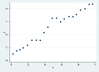
Figure 1: Canonical Binned Scatter Plot.

By default, the command binsreg evaluates and plots the regression function of interest $\vartheta^{(v)}_{\mathbf{w}}(x)$ at the mean of the additional covariates $\mathbf{w}_{i}$, i.e., $\mathbf{w}=\bar{\mathbf{w}}$. Users may specify a different value of $\mathbf{w}$, for example, the empirical median of each component in $\mathbf{w}_{i}$, via the option at():

. binsreg y x w, at(median)

Users may also save the values of the additional covariates at which the binscatter estimate is evaluated in another file, and then specify the file name in the option at(). For example,

• 
  

  . tempfile evalcovar
  
  . preserve
  
  . clear
  
  . set obs 1
  number of observations (_N) was 0, now 1
  
  . gen w=0.2
  
  . gen t=1
  
  . save `evalcovar´, replace
  (note: file C:\Users\y\AppData\Local\Temp\ST_4fa0_000001.tmp not found)
  file C:\Users\y\AppData\Local\Temp\ST_4fa0_000001.tmp saved
  
  . restore
  
  . binsreg y x w i.t, at(`evalcovar´)
  Sorting dataset on x...
  Note: This step is omitted if dataset already sorted by x.
  
  Binscatter plot
  Bin selection method: IMSE-optimal plug-in choice (select # of bins)
  Placement: Quantile-spaced
  Derivative: 0
  
                                                 
  # of observations                  1000
  # of distinct values               1000
  # of clusters                         .
                                                 
  Bin/Degree selection:          
           Degree of polynomial         0
    # of smoothness constraints         0
                      # of bins        22
                   imse, bias^2     4.736
                     imse, var.     0.974
                                                 
  
                                           
                  p       s       df
                                           
   dots           0       0       22
                                           
  

In this case, we control for a continuous variable w and a dummy variable generated based on the binary covariate t. We evaluate the binscatter estimate at w=0.2 and t=1, and these values are saved in the temporary file ‘evalcovar’ in advance.

Users may specify the number of bins manually rather than relying on the automatic data-driven procedures. For example, a popular ad-hoc choice in practice is setting $J=20$ quantile-spaced bins:

• 
  

  . binsreg y x w, nbins(20) polyreg(1)
  Sorting dataset on x...
  Note: This step is omitted if dataset already sorted by x.
  Note: When additional covariates w are included, the polynomial fit may not always be clos
  > e to the binscatter fit.
  
  Binscatter plot
  Bin selection method: User-specified
  Placement: Quantile-spaced
  Derivative: 0
  
                                                 
  # of observations                  1000
  # of distinct values               1000
  # of clusters                         .
                                                 
  Bin/Degree selection:          
           Degree of polynomial         0
    # of smoothness constraints         0
                      # of bins        20
                                                 
  
                                           
                  p       s       df
                                           
   dots           0       0       20
   polyreg        1       NA      2
                                           
  

The option polyreg(1) adds a linear prediction line to the canonical binscatter plot, but the resulting binned scatter plot is not reported here to conserve space.

Figure 2: Binned Scatter Plot with Lines, Confidence Intervals and Bands.

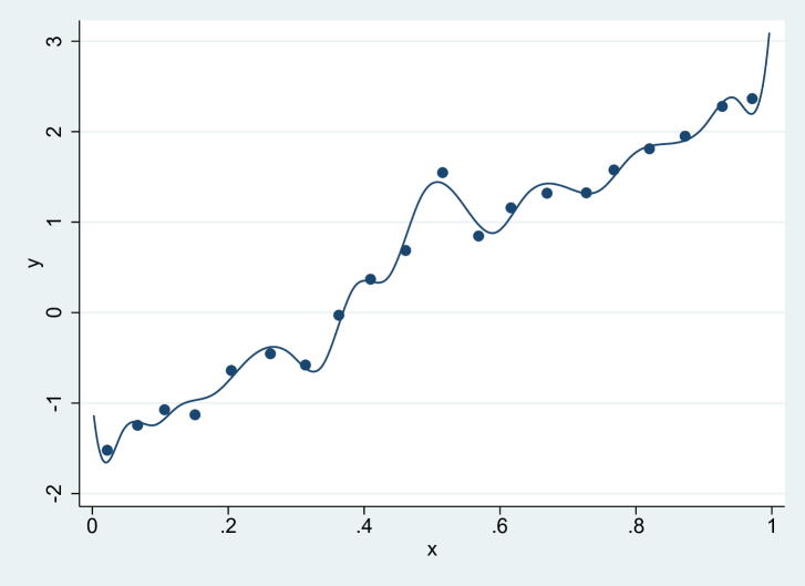
(a) Add cubic $B$-spline fit

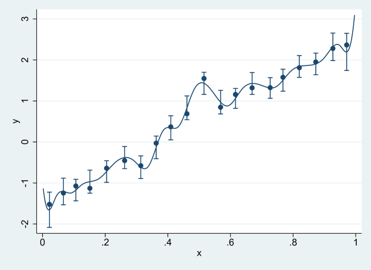
(b) Add confidence intervals

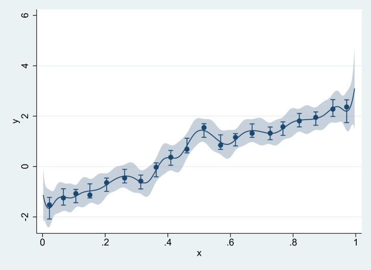
(c) Add confidence band

(d) Add a polynomial fit of degree $4$

The command binsreg allows users to add a binscatter-based line approximating the unknown regression function, pointwise confidence intervals, a uniform confidence band, and a global polynomial regression approximation. For example, the following syntax cumulatively adds in four distinct plots a fitted line, confidence intervals and a confidence band, all three based on cubic $B$-splines, and also a fitted line based on a global polynomial of degree $4$. The results are shown in Figure 2.

• 
  

  . qui binsreg y x w, nbins(20) dots(0,0) line(3,3)
  
  . qui binsreg y x w, nbins(20) dots(0,0) line(3,3) ci(3,3)
  
  . qui binsreg y x w, nbins(20) dots(0,0) line(3,3) ci(3,3) cb(3,3)
  
  . qui binsreg y x w, nbins(20) dots(0,0) line(3,3) ci(3,3) cb(3,3) polyreg(4)
  
  

By construction, a cubic $B$-spline fit is a piecewise cubic polynomial function which is continuous, and has continuous first- and second-order derivatives. Thus, the prediction line and confidence band generated are quite smooth. In this case, it is arguably under-smoothed because of the “large” choice of $J=20$. The degree and smoothness of polynomials can be changed by adjusting the values of p and s in the options dots(), line(), ci() and cb().

The command binsreg also allows for the standard vce options, factor variables, and twoway graph options, among other features. This is illustrated in the following code:

• 
  

  . binsreg y x w i.t, dots(0,0) line(3,3) ci(3,3) cb(3,3) polyreg(4) ///
  >                    vce(cluster id) savedata(output/graphdat) replace ///
  >                                    title("Binned Scatter Plot")
  Sorting dataset on x...
  Note: This step is omitted if dataset already sorted by x.
  Note: When additional covariates w are included, the polynomial fit may not always be clos
  > e to the binscatter fit.
  Note: Setting at least nsims(2000) and simsgrid(50) is recommended to obtain the final res
  > ults.
  
  Binscatter plot
  Bin selection method: IMSE-optimal plug-in choice (select # of bins)
  Placement: Quantile-spaced
  Derivative: 0
  Output file: output/graphdat.dta
  
                                                 
  # of observations                  1000
  # of distinct values               1000
  # of clusters                       500
                                                 
  Bin/Degree selection:          
           Degree of polynomial         0
    # of smoothness constraints         0
                      # of bins        20
                   imse, bias^2     3.588
                     imse, var.     0.494
                                                 
  
                                           
                  p       s       df
                                           
   dots           0       0       20
   line           3       3       23
   CI             3       3       23
   CB             3       3       23
   polyreg        4       NA      5
                                           
  

Specifically, a dummy variable based on the binary covariate t is added to the estimation, standard errors are clustered at the group level indicator id, and a graph title is added to the resulting binned scatter plot. Note that any unrecognized options for the command binsreg will be understood as twoway options and therefore appended to the final plot command. Thus, users may easily modify, for example, axis properties, legends, etc. The option savedata(graphdat) saves the underlying data used in the binned scatter plot in the file graphdat.dta.

In addition, the command binsreg can be used for subgroup analysis. The following command implements binscatter estimation and inference across two subgroups separately, defined by the variable t, and then produces a common binned scatter plot (Figure 3):

• 
  

  . binsreg y x w, by(t) dots(0,0) line(3,3) cb(3,3) ///
  >                bycolors(blue red) bysymbols(O T)
  Sorting dataset on x...
  Note: This step is omitted if dataset already sorted by x.
  Note: Setting at least nsims(2000) and simsgrid(50) is recommended to obtain the final res
  > ults.
  
  Binscatter plot
  Bin selection method: IMSE-optimal plug-in choice (select # of bins)
  Placement: Quantile-spaced
  Derivative: 0
  
  Group: t = 0
                                                 
  # of observations                   485
  # of distinct values                485
  # of clusters                         .
                                                 
  Bin/Degree selection:          
           Degree of polynomial         0
    # of smoothness constraints         0
                      # of bins        20
                   imse, bias^2     7.107
                     imse, var.     0.942
                                                 
  
                                           
                  p       s       df
                                           
   dots           0       0       20
   line           3       3       23
   CB             3       3       23
                                           
  Note: Setting at least nsims(2000) and simsgrid(50) is recommended to obtain the final res
  > ults.
  
  
  Group: t = 1
                                                 
  # of observations                   515
  # of distinct values                515
  # of clusters                         .
                                                 
  Bin/Degree selection:          
           Degree of polynomial         0
    # of smoothness constraints         0
                      # of bins        15
                   imse, bias^2     2.861
                     imse, var.     0.955
                                                 
  
                                           
                  p       s       df
                                           
   dots           0       0       15
   line           3       3       18
   CB             3       3       18
                                           
  

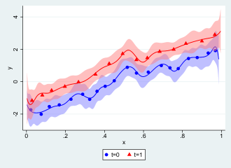
Figure 3: Binned Scatter Plot: Group Comparison

Figure 3 highlights a difference across the two subgroups defined by the variable t, which corresponds to the fact that our simulated data add a $1$ to the outcome variable for those units with $\mathtt{t=1}$. The colors, symbols, and line patterns in Figure 3 can be modified via the options bycolors(), bysymbols(), and bylpatterns(). When the number of bins is unspecified, the command binsreg selects the number of bins for each subsample separately, via the companion command binsregselect. This means that, by default, the choice of binning/partitioning structure will be different across subgroups in general. However, if the option samebinsby is specified, then a common binning scheme for all subgroups is constructed based on the full sample.

As described before, sometimes one would like to keep the number of bins $J$ fixed and select the degree/smoothness of the polynomial instead. The following snippet illustrates how to implement this procedure:

• 
  

  . binsreg y x w, nbins(20) line(T) ci(T) cb(T) pselect(0/3)
  Sorting dataset on x...
  Note: This step is omitted if dataset already sorted by x.
  Note: Setting at least nsims(2000) and simsgrid(50) is recommended to obtain the final res
  > ults.
  
  Binscatter plot
  Bin selection method: IMSE-optimal plug-in choice (select degree and smoothness)
  Placement: Quantile-spaced
  Derivative: 0
  
                                                 
  # of observations                  1000
  # of distinct values               1000
  # of clusters                         .
                                                 
  Bin/Degree selection:          
           Degree of polynomial         0
    # of smoothness constraints         0
                      # of bins        20
                   imse, bias^2     5.422
                     imse, var.     1.181
                                                 
  
                                           
                  p       s       df
                                           
   dots           0       0       20
   line           0       0       20
   CI             1       1       21
   CB             1       1       21
                                           
  

Here we let $J=20$ and select the degree of polynomial $p$ within the specified range $\{0,1,2,3\}$. The resulting optimal $p$ is 0. Accordingly, we construct “dots”, “line” based on piecewise constant estimates, and confidence intervals and a confidence band based on linear spline estimates.

The accompanying replication files include other illustrations. For example:

• Inference based on asymptotic variance formula:
  . binsreg y x w i.t, dots(0,0) line(3,3) ci(3,3) cb(3,3) polyreg(4) vce(cluster id) asyvar(on)

• Using the community-contributed module reghdfe:
  . binsreg y x w, absorb(t) dots(0,0) line(3,3) ci(3,3) cb(3,3) polyreg(4)

• Turning off data distribution robustness checks and using the community-contributed module gtools:
  . binsreg y x w, masspoints(off) usegtools(on)

Next, we illustrate the command binsqreg for estimation and uncertainty quantification using quantile regression binscatter methods. The following code looks at the conditional $25$-th quantile of the outcome variable.

• 
  

  . binsqreg y x w, quantile(0.25)
  Sorting dataset on x...
  Note: This step is omitted if dataset already sorted by x.
  
  Binscatter plot, quantile
  Bin selection method: IMSE-optimal plug-in choice (select # of bins)
  Placement: Quantile-spaced
  Derivative: 0
  
                                                 
  # of observations                  1000
  # of distinct values               1000
  # of clusters                         .
                                                 
  Bin/Degree selection:          
           Degree of polynomial         0
    # of smoothness constraints         0
                      # of bins        21
                   imse, bias^2     5.420
                     imse, var.     1.192
                                                 
  
                                           
                  p       s       df
                                           
   dots           0       0       21
                                           
  

By default, quantile regression methods employ an analytic variance estimator formula, which may not perform well in applications. A more robust alternative is employing bootstrap methods:

• 
  

  . binsqreg y x w, quantile(0.25) ci(3 3) vce(bootstrap, reps(100))
  Sorting dataset on x...
  Note: This step is omitted if dataset already sorted by x.
  
  Binscatter plot, quantile
  Bin selection method: IMSE-optimal plug-in choice (select # of bins)
  Placement: Quantile-spaced
  Derivative: 0
  
                                                 
  # of observations                  1000
  # of distinct values               1000
  # of clusters                         .
                                                 
  Bin/Degree selection:          
           Degree of polynomial         0
    # of smoothness constraints         0
                      # of bins        21
                   imse, bias^2     5.420
                     imse, var.     1.192
                                                 
  
                                           
                  p       s       df
                                           
   dots           0       0       21
   CI             3       3       24
                                           
  

The replication files also illustrate how to plot together least squares and quantile regression binscatter approximations. The final output is illustrated in Figure 4, which plots the conditional mean and its confidence band, together with the conditional $25$-th and $75$-th quantile regressions (i.e., conditional inter-quartile range).

Figure 4: Binned Scatter Plot for Means and Quantiles.

Moreover, we provide a convenient option qregopt(qreg_option) to modify the underlying quantile regression. For example, the user can control for the optimization process as follows:

• 
  

  . qui binsqreg y x w, quantile(0.25) qregopt(iterate(1000) wls(1))
  
  

Finally, we illustrate the command binslogit for binary response regression binscatter methods using logistic regression.

• 
  

  . binslogit d x w
  Sorting dataset on x...
  Note: This step is omitted if dataset already sorted by x.
  
  Binscatter plot, logit model
  Bin selection method: IMSE-optimal plug-in choice (select # of bins)
  Placement: Quantile-spaced
  Derivative: 0
  
                                                 
  # of observations                  1000
  # of distinct values               1000
  # of clusters                         .
                                                 
  Bin/Degree selection:          
           Degree of polynomial         0
    # of smoothness constraints         0
                      # of bins        12
                   imse, bias^2     0.172
                     imse, var.     0.208
                                                 
  
                                           
                  p       s       df
                                           
   dots           0       0       12
                                           
  

4.2 Hypothesis Testing and Statistical Inference

We illustrate first the syntax and outputs of the command binstest. The basic syntax is the following:

• 
  

  . binstest y x w, testmodelpoly(1)
  Note: Setting at least nsims(2000) and simsgrid(50) is recommended to obtain the final res
  > ults.
  
  Hypothesis tests based on binscatter estimates
  Estimation method: reg
  Bin selection method: IMSE-optimal plug-in choice (select # of bins)
  Placement: Quantile-spaced
  Derivative: 0
  
                                                 
  # of observations                  1000
  # of distinct values               1000
  # of clusters                         .
                                                 
  Bin/Degree selection:          
           Degree of polynomial         0
    # of smoothness constraints         0
                      # of bins        21
                                                 
  
  Model specification Tests:
  Degree: 1     # of smoothness constraints: 1
  
                                                     
  H0: mu =             sup |T|           p value
                                                     
  poly. degree  1        6.566             0.000
                                                     
  

A test for linearity of the regression function $\mu_{0}(x)$ is implemented using the binscatter estimator. By default, a linear $B$-spline is employed in the inference procedure, which can be adjusted by the option testmodel(). In addition, when unspecified, the number of bins is selected using a data-driven procedure via the companion command binsregselect. The selected number of bins is IMSE-optimal for piecewise constant point estimates by default. A summary of the sample and binning scheme is displayed, and then the test statistic and p-value are reported. In this case, the test statistic is the supremum of the absolute value of the $t$-statistic evaluated over a sequence of grid points, and the p-value is calculated based on simulation. Clearly, the p-value is quite small, and thus the null hypothesis of linearity of the regression function is rejected.

As emphasized before, the parametric specification test for a null hypothesis about the level may be sensitive to the choice of evaluation point $\mathbf{w}$. Thus, a recommended strategy to test for linearity of $\mu_{0}(x)$ is to check if its first derivative is a constant, which is implemented in the following:

• 
  

  . binstest y x w, testmodelpoly(1) deriv(1)
  Note: Setting at least nsims(2000) and simsgrid(50) is recommended to obtain the final res
  > ults.
  
  Hypothesis tests based on binscatter estimates
  Estimation method: reg
  Bin selection method: IMSE-optimal plug-in choice (select # of bins)
  Placement: Quantile-spaced
  Derivative: 1
  
                                                 
  # of observations                  1000
  # of distinct values               1000
  # of clusters                         .
                                                 
  Bin/Degree selection:          
           Degree of polynomial         1
    # of smoothness constraints         1
                      # of bins         6
                                                 
  
  Model specification Tests:
  Degree: 2     # of smoothness constraints: 2
  
                                                     
  H0: mu =             sup |T|           p value
                                                     
  poly. degree  1        4.114             0.000
                                                     
  

Note that for $v=1$, the selected number of bins is IMSE-optimal for the linear $B$-spline estimate by default, and the test statistic based on the proposed robust bias correction strategy is constructed using a quadratic $B$-spline fit.

The command binstest can implement testing for any parametric model specification by comparing the fitted values based on the binscatter estimator (computed by the command) and the parametric model of interest (provided by the user). For example, the following code creates an auxiliary database with a grid of evaluation points, implements a linear regression first, makes an out-of-sample prediction using the auxiliary dataset, and then tests for linearity based on the binscatter estimator by specifying the auxiliary file containing the fitted values.

• 
  

  . qui binsregselect y x w, simsgrid(30) savegrid(output/parfitval) replace
  
  . qui reg y x w
  
  . use output/parfitval, clear
  
  . predict binsreg_fit_lm
  (option xb assumed; fitted values)
  
  . save output/parfitval, replace
  file output/parfitval.dta saved
  
  . use binsreg_simdata, clear
  
  . binstest y x w, testmodelparfit(output/parfitval) lp(2) deriv(1)
  Note: Setting at least nsims(2000) and simsgrid(50) is recommended to obtain the final res
  > ults.
  
  Hypothesis tests based on binscatter estimates
  Estimation method: reg
  Bin selection method: IMSE-optimal plug-in choice (select # of bins)
  Placement: Quantile-spaced
  Derivative: 1
  
                                                 
  # of observations                  1000
  # of distinct values               1000
  # of clusters                         .
                                                 
  Bin/Degree selection:          
           Degree of polynomial         1
    # of smoothness constraints         1
                      # of bins         6
                                                 
  
  Model specification Tests:
  Degree: 2     # of smoothness constraints: 2
  
  Input file: output/parfitval.dta
                                                     
  H0: mu =             L2 of T           p value
                                                     
     binsreg_fit_lm      4.377             0.000
                                                     
  

The first line, binsregselect y x w, simsgrid(30) savegrid(output/parfitval) replace, generates the auxiliary file containing the grid of evaluation points. Since the parameter of interest is only the mean relation between y and x, i.e., $\mu_{0}(x)$, at the out-of-sample prediction step, the testing dataset parfitval.dta must contain a variable x containing a sequence of evaluation points at which the binscatter and parametric models are compared, and the covariate w whose values are set as zeros. In addition, the variable containing fitted values has to follow a specific naming rule, i.e., takes the form of binsreg_fit*. The companion command binsregselect can be used to construct the required auxiliary dataset, as illustrated above. We discuss this other command further below.

In addition to model specification tests, the command binstest can test for nonparametric shape restrictions on the regression function. For example, the following syntax tests whether the regression function is increasing:

• 
  

  . binstest y x w, deriv(1) nbins(20) testshaper(0)
  Warning: Testing procedures are valid when nbins() is much larger than the IMSE-optimal ch
  > oice. Compare your choice with the IMSE-optimal one obtained by binsregselect.
  Note: Setting at least nsims(2000) and simsgrid(50) is recommended to obtain the final res
  > ults.
  
  Hypothesis tests based on binscatter estimates
  Estimation method: reg
  Bin selection method: User-specified
  Placement: User-specified
  Derivative: 1
  
                                                 
  # of observations                  1000
  # of distinct values               1000
  # of clusters                         .
                                                 
  Bin/Degree selection:          
           Degree of polynomial         .
    # of smoothness constraints         .
                      # of bins        20
                                                 
  
  Shape Restriction Tests:
  Degree: 2     # of smoothness constraints: 2
  
                                                     
  H0: inf mu >=        inf T             p value
                                                     
           0            -3.709             0.004
                                                     
  

The null hypothesis here is that the infimum of the first-order derivative of the regression function is no less than $0$. The output reports the test statistic, which is the infimum of the $t$-statistic over a sequence of evaluation points, and the corresponding simulation-based p-value.

The command binstest may implement many tests simultaneously (given the derivative of interest). For example,

• 
  

  . binstest y x w, nbins(20) testshaper(-2 0) testshapel(4) testmodelpoly(1) ///
  >                    nsims(1000) simsgrid(30)
  Warning: Testing procedures are valid when nbins() is much larger than the IMSE-optimal ch
  > oice. Compare your choice with the IMSE-optimal one obtained by binsregselect.
  Note: Setting at least nsims(2000) and simsgrid(50) is recommended to obtain the final res
  > ults.
  
  Hypothesis tests based on binscatter estimates
  Estimation method: reg
  Bin selection method: User-specified
  Placement: User-specified
  Derivative: 0
  
                                                 
  # of observations                  1000
  # of distinct values               1000
  # of clusters                         .
                                                 
  Bin/Degree selection:          
           Degree of polynomial         .
    # of smoothness constraints         .
                      # of bins        20
                                                 
  
  Shape Restriction Tests:
  Degree: 1     # of smoothness constraints: 1
  
                                                     
  H0: sup mu <=        sup T             p value
                                                     
           4            -4.131             1.000
                                                     
  
                                                     
  H0: inf mu >=        inf T             p value
                                                     
           -2            1.774             1.000
           0           -10.772             0.000
                                                     
  
  Model specification Tests:
  Degree: 1     # of smoothness constraints: 1
  
                                                     
  H0: mu =             sup |T|           p value
                                                     
  poly. degree  1        5.972             0.000
                                                     
  

The above syntax tests three shape restrictions and one model specification (linearity), employing 1000 random draws from $\mathbf{N}_{K}^{\star}$ and $30$ evaluation points to evaluate the supremum/infimum in the simulation.

The accompanying replication files include other illustrations. For example:

• Testing whether the median regression function is linear:
  . binstest y x w, estmethod(qreg 0.5) testmodelpoly(1)

• Testing whether the nonlinear logistic regression function is increasing:
  . binstest d x w, estmethod(logit) deriv(1) nbins(20) testshaper(0)

Next, consider pairwise comparison as implemented via the testing command binspwc. Using least square binscatter for the two samples identified via the binary variable t, we have:

• 
  

  . binspwc y x w, by(t)
  Note: Setting at least nsims(2000) and simsgrid(50) is recommended to obtain the final res
  > ults.
  
  Pairwise group comparison based on binscatter estimates
  Estimation method: reg
  Derivative: 0
  Group variable: t
  Bin/Degree selection method: IMSE-optimal plug-in choice (select # of bins)
  Placement: Quantile-spaced
  
  Group 1 vs. Group 0
                                                        
  Group t=                             1         0
                                                        
  # of observations                   515        485
  # of distinct values                515        485
  # of clusters                         .          .
  Degree of polynomial                  1          1
  # of smoothness constraints           1          1
  # of bins                            15         20
                                                       
  
  diff = group 1 - group 0
                                                     
  H0:                  sup |T|           p value
                                                     
  diff=0                 5.790             0.000
                                                     
  
  

Similarly, employing quantile regression binscatter methods, for the $40$-th conditional quantile of the outcome variable, we have

• 
  

  . binspwc y x w, by(t) estmethod(qreg 0.4)
  Note: Setting at least nsims(2000) and simsgrid(50) is recommended to obtain the final res
  > ults.
  
  Pairwise group comparison based on binscatter estimates
  Estimation method: qreg
  Derivative: 0
  Group variable: t
  Bin/Degree selection method: IMSE-optimal plug-in choice (select # of bins)
  Placement: Quantile-spaced
  
  Group 1 vs. Group 0
                                                        
  Group t=                             1         0
                                                        
  # of observations                   515        485
  # of distinct values                515        485
  # of clusters                         .          .
  Degree of polynomial                  1          1
  # of smoothness constraints           1          1
  # of bins                            15         20
                                                       
  
  diff = group 1 - group 0
                                                     
  H0:                  sup |T|           p value
                                                     
  diff=0                 5.023             0.000
                                                     
  
  

4.3 Binning Selection

As already mentioned, the commands binsreg and binstest rely on data-driven bin selection procedures via the command binsregselect whenever the option nbins() is not employed by the user. Its basic syntax is as follows:

• 
  

  . binsregselect y x w
  
  Bin selection for binscatter estimates
  Method: IMSE-optimal plug-in choice (select # of bins)
  Position: Quantile-spaced
  
                                          
            # of observations      1000
         # of distince values      1000
                # of clusters         .
             eff. sample size      1000
                                          
         Degree of polynomial         0
   # of smoothness constraint         0
                                          
  
                                                                          
      method       # of bins       df     imse, bias^2    imse, var.
                                                                          
     ROT-POLY          18          18        3.295          1.212
     ROT-REGUL         18          18            .              .
     ROT-UKNOT         18          18            .              .
        DPI            21          21        5.420          1.192
     DPI-UKNOT         21          21            .              .
                                                                          
  df: degrees of freedom.
  

The following choices of number of bins are reported: ROT-POLY, the rule-of-thumb (ROT) choice based on global polynomial estimation; ROT-REGUL, the ROT choice regularized as discussed in Section 2, or the user’s choice specified in the option nbinsrot(); ROT-UKNOT, the ROT choice with unique knots; DPI, the direct plug-in (DPI) choice; and DPI-UKNOT, the DPI choice with unique knots.

The direct plug-in choice is implemented based on the rule-of-thumb choice, which can be set by users directly:

• 
  

  . binsregselect y x w, nbinsrot(20) binspos(es)
  
  Bin selection for binscatter estimates
  Method: IMSE-optimal plug-in choice (select # of bins)
  Position: Evenly-spaced
  
                                          
            # of observations      1000
         # of distince values      1000
                # of clusters         .
             eff. sample size      1000
                                          
         Degree of polynomial         0
   # of smoothness constraint         0
                                          
  
                                                                          
      method       # of bins       df     imse, bias^2    imse, var.
                                                                          
     ROT-POLY           .           .            .              .
     ROT-REGUL         20          20            .              .
     ROT-UKNOT         20          20            .              .
        DPI            22          22        5.793          1.194
     DPI-UKNOT         22          22            .              .
                                                                          
  df: degrees of freedom.
  

Notice that in the example above an evenly-spaced, rather than quantile-spaced, binning scheme is selected via the option binspos(es). The binning used in the commands binsreg and binstest may be adjusted similarly.

In addition, as illustrated above, the command binsregselect also provides a convenient option savegrid(), which can be used to generate the auxiliary dataset needed for parametric specification testing of user-chosen models via the command binstest. Specifically, the following command was (quietly) used above:

• 
  

  . binsregselect y x w, simsgrid(30) savegrid(output/parfitval) replace
  
  Bin selection for binscatter estimates
  Method: IMSE-optimal plug-in choice (select # of bins)
  Position: Quantile-spaced
  Output file: output/parfitval.dta
  
                                          
            # of observations      1000
         # of distince values      1000
                # of clusters         .
             eff. sample size      1000
                                          
         Degree of polynomial         0
   # of smoothness constraint         0
                                          
  
                                                                          
      method       # of bins       df     imse, bias^2    imse, var.
                                                                          
     ROT-POLY          18          18        3.295          1.212
     ROT-REGUL         18          18            .              .
     ROT-UKNOT         18          18            .              .
        DPI            21          21        5.420          1.192
     DPI-UKNOT         21          21            .              .
                                                                          
  df: degrees of freedom.
  

The resulting file, parfitval.dta, includes x and w as well as some other variables related to the binning scheme. The variable x contains a sequence of evaluation points, in this case set to $30$ within each bin via the option simsgrid(), and the values of w are set to zero on purpose (this is used to generate the fitting model correctly).

When an extremely large dataset is available, the data-driven procedures for selecting the binning scheme could be very time-consuming. In such a scenario, one could use a small sub-sample to estimate the leading constants in the integrated mean squared error (IMSE) expansions, and then extrapolate the optimal number of bins to the full sample. The following code illustrates how this method is implemented:

• 
  

  . binsregselect y x w if t==0, useeffn(1000)
  
  Bin selection for binscatter estimates
  Method: IMSE-optimal plug-in choice (select # of bins)
  Position: Quantile-spaced
  
                                          
            # of observations       485
         # of distince values       485
                # of clusters         .
             eff. sample size      1000
                                          
         Degree of polynomial         0
   # of smoothness constraint         0
                                          
  
                                                                          
      method       # of bins       df     imse, bias^2    imse, var.
                                                                          
     ROT-POLY          20          20        3.185          0.937
     ROT-REGUL         20          20            .              .
     ROT-UKNOT         20          20            .              .
        DPI            26          26        7.107          0.942
     DPI-UKNOT         26          26            .              .
                                                                          
  df: degrees of freedom.
  

In this example $485$ observations with $\mathtt{t=0}$ are used to compute the leading constants $\mathscr{B}_{n}(p,s,v)$ and $\mathscr{V}_{n}(p,s,v)$ in the IMSE expansion, but then the reported optimal numbers of bins are calculated based on the effective sample size specified in the option useeffn(). This method also applies to extrapolating the optimal number of bins to a smaller sample based on a larger one.

Alternatively, the number of bins selection can be implemented using only a random sub-sample of the observations. For example, the following command selects $J$ using, in expectation, $30\%$ of the observations based on uniformly distributed random numbers. Repeated application of this command will produce modestly different bins selection choices depending on the sequence of realized uniform random variables.

• 
  

  . binsregselect y x w, randcut(0.3)
  
  Bin selection for binscatter estimates
  Method: IMSE-optimal plug-in choice (select # of bins)
  Position: Quantile-spaced
  
                                          
            # of observations      1000
         # of distince values      1000
                # of clusters         .
             eff. sample size      1000
                                          
         Degree of polynomial         0
   # of smoothness constraint         0
                                          
  
                                                                          
      method       # of bins       df     imse, bias^2    imse, var.
                                                                          
     ROT-POLY          18          18        3.714          1.303
     ROT-REGUL         18          18            .              .
     ROT-UKNOT         18          18            .              .
        DPI            23          23        7.104          1.289
     DPI-UKNOT         23          23            .              .
                                                                          
  df: degrees of freedom.
  

5 Conclusion

We introduced the Stata package Binsreg, which provides general-purpose software implementations of binscatter via seven commands: (i) binsreg, binslogit, binsprobit, binsqreg for point estimation, uncertainty quantification and binned scatter plotting in least squares, Logit, Probit and quantile regression settings; (ii) binstest for hypothesis testing and statistical inference for parametric specification and nonparametric shape restrictions, and binspwc for multi-group pairwise statistical comparisons; and (iii) binsregselect for binning scheme selection. All our methods allow for multi-sample comparisons, which is useful when studying treatment effects heterogeneity in randomized and observational studies. Companion Python and R packages with similar syntax and capabilities are also available.

6 Acknowledgments

We thank Michael Droste, John Friedman, Andreas Fuster, Filippo Palomba, Paul Goldsmith-Pinkham, David Lucca, Xinwei Ma, Ricardo Masini, Jonah Rockoff, Jesse Rothstein, Ryan Santos, Jesse Shapiro, and Rocio Titiunik for helpful comments and discussions.

Cattaneo gratefully acknowledges financial support from the National Science Foundation through grants SES-1947805, SES-2019432, and SES-2241575.

7 About the Authors

Matias D. Cattaneo is a Professor of Operations Research and Financial Engineering at Princeton University.

Richard K. Crump is a Financial Research Advisor in Macrofinance Studies at the Federal Reserve Bank of New York.

Max H. Farrell is an Associate Professor of Economics at the University of California at Santa Barbara.

Yingjie Feng is an Assistant Professor of Economics at Tsinghua University.

References

- Caceres (2023) Caceres, M. 2023. Stata Module Mauricio https://github.com/mcaceresb/stata-gtools.
- Calonico et al. (2018) Calonico, S., M. D. Cattaneo, and M. H. Farrell. 2018. On the Effect of Bias Estimation on Coverage Accuracy in Nonparametric Inference. Journal of the American Statistical Association 113(522): 767–779.
- Calonico et al. (2022) . 2022. Coverage Error Optimal Confidence Intervals for Local Polynomial Regression. Bernoulli 28(4): 2998–3022.
- Calonico et al. (2014) Calonico, S., M. D. Cattaneo, and R. Titiunik. 2014. Robust Nonparametric Confidence Intervals for Regression-Discontinuity Designs. Econometrica 82(6): 2295–2326.
- Cattaneo et al. (2023a) Cattaneo, M. D., R. K. Crump, M. H. Farrell, and Y. Feng. 2023a. On Binscatter. arXiv:1902.09608 .
- Cattaneo et al. (2023b) . 2023b. Nonlinear Binscatter Methods. working paper .
- Cattaneo et al. (2020) Cattaneo, M. D., M. H. Farrell, and Y. Feng. 2020. Large sample properties of partitioning-based series estimators. Annals of Statistics 48(3): 1718–1741.
- Correia and Constantine (2023) Correia, S., and N. Constantine. 2023. Stata Module reghdfe https://github.com/sergiocorreia/reghdfe.
- Droste (2019) Droste, M. 2019. Stata Module Binscatter2 https://github.com/mdroste/stata-binscatter2/.
- Starr and Goldfarb (2020) Starr, E., and B. Goldfarb. 2020. Binned Scatterplots: A Simple Tool to Make Research Easier and Better. Strategic Management Journal 41(12): 2261–2274.
- Stepner (2017) Stepner, M. 2017. Stata Module Binscatter https://github.com/michaelstepner/binscatter/.