Abstract

In this work we introduce a class of dynamic models for time series taking values on the unit interval. The proposed model follows a generalized linear model approach where the random component, conditioned on the past information, follows a beta distribution, while the conditional mean specification may include covariates and also an extra additive term given by the iteration of a map that can present chaotic behavior. The resulting model is very flexible and its systematic component can accommodate short and long range dependence, periodic behavior, laminar phases, etc. We derive easily verifiable conditions for the stationarity of the proposed model, as well as conditions for the law of large numbers and a Birkhoff-type theorem to hold. A Monte Carlo simulation study is performed to assess the finite sample behavior of the partial maximum likelihood approach for parameter estimation in the proposed model. Finally, an application to the proportion of stored hydroelectrical energy in Southern Brazil is presented.
Keywords: time series; chaotic processes; generalized linear models.
2010 Mathematical Subject Classification: Primary: 37M10, 62M10, 62J12.

1 Introduction

Many time series encountered in statistical applications present two important characteristics: bounds, in the sense that its distribution has a bounded support, and serial dependence. Common cases are rates and proportions observed over time. In these cases, Gaussian based approaches are not adequate. Time series modeling of double bounded time series has been subject of intense research, especially in the last decade, and several approaches to the problem have been proposed. One such approach has received a lot of attention in the last few years. The idea is to include a time dependent structure into a Generalized Linear Model (GLM) framework and has been popularized in the works of Zeger and Qaqish (1988), Benjamin et al. (2003) and Ferrari and Cribari-Neto (2004). Processes following this type of structure are often referred to as Generalized Autoregressive Moving Average (GARMA) models. More specifically, the model’s systematic component follows the usual approach of GLM with an additional dynamic term of the form

$$g(\mu_{t})={\eta}_{t}=\boldsymbol{x}_{t}^{\prime}\boldsymbol{\beta}+\tau_{t},$$ (1)

where $g$ is a suitable link function, $\mu_{t}$ is some quantity of interest (usually the (un)conditional mean or median), $\boldsymbol{x}_{t}$ denotes a vector of (possibly random) covariates observed at time $t$ and $\tau_{t}$ is a term responsible to accommodate any serial correlation in the sequence $\mu_{t}$. The term $\tau_{t}$ can take a variety of forms, depending on the model’s scope and intended application. In the Beta Autoregressive Moving Average ($\beta$ARMA) model (Rocha and Cribari-Neto, 2009), for instance, the model’s random component follows a (conditional) beta distribution while in the specification for the conditional mean $\mu_{t}$, $\tau_{t}$ follows a classical ARMA process. In Bayer et al. (2017), the authors define the Kumaraswamy ARMA model (KARMA), where the model’s random component follows a (conditional) Kumaraswamy distribution while in the specification for the conditional median $\mu_{t}$, $\tau_{t}$ also follows an ARMA process. Since ARMA models can only accommodate short range dependence, these models can only account for a short range dependence structure on their systematic component. In the case of conditionally beta distributed random component, Pumi et al. (2019) introduce the $\beta$ARFIMA (Beta Autoregressive Fractionally Integrated Moving Average) model generalizing Rocha and Cribari-Neto (2009) by allowing $\tau_{t}$ to follow a long range dependent ARFIMA process (see, for instance, Honsking, 1981; Brockwell and Davis, 1991; Palma, 2007; Box et al., 2008). Inference for this type of models is done via partial maximum likelihood.

In this work we propose a model where the random component follows a conditional beta distribution, while the systematic component depends on the iterations of a (usually chaotic) map defined on the unit interval. Let $T:[0,1]\rightarrow[0,1]$ and $U_{0}$ be a random variable taking values in $(0,1)$, in particular, provided the existence of an absolute continuous invariant measure for $T$, $U_{0}$ will be distributed according to it (see Section 2.2). We consider the so-called class of chaotic process defined by setting $Z_{t}:=h\big{(}T^{t}(U_{0})\big{)}$, $t\in\mathds{N}$, for a suitably smooth link function $h:(0,1)\rightarrow\mathds{R}$. A key concept here is the one of invariant measure for a map $T$: provided an absolute continuous invariant measure exists, $U_{0}$ will be distributed according to it (see Section 2.2). Observe that $T$ does not need to be a chaotic transformation in the usual sense (see next section) for $Z_{t}$ to be called a chaotic process. Such processes have been applied in a variety of problems from rock drilling (see Lasota and Yorke, 1973, and references therein) to intermittency in human cardiac rate (see Zebrowsky, 2001), econometrics (Gandolfo, 2009), biology and medicine (Jackson and Radunskaya, 2015), etc. However, the goal on these applications usually lie on understanding the dynamics of the process (i.e., intermittence, presence of fixed/attracting/repelling points, invariant measures, etc) rather than statistical inference or forecasting.

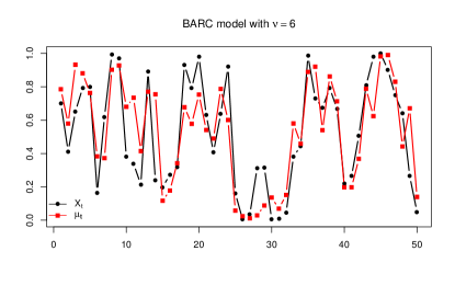
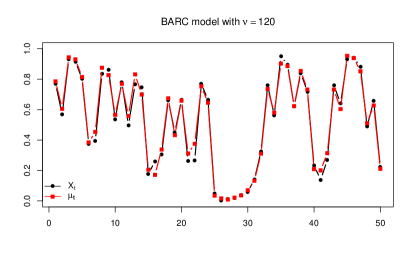
Figure 1: In (a) and (b) we present the sample paths (black) and conditional mean $\mu_{t}$ (red) of two $\beta$ARC(1) models obtained from the Mannevile-Pomeau transformation starting at $u_{0}=\pi/4$ with parameters parameter $\phi=0.3$ and $s=0.3$. In (a) we have $\nu=6$ while in (b) $\nu=120$.

The novelty of the proposed model lies in 3 different fronts: first, its capability of modeling non-linear behaviors that other GARMA-like models can’t; second, its flexibility; and finally, general theoretical results that are not available for other GARMA-like models in the literature can be obtained for $\beta$ARC models under easily verifiable conditions.

Upon changing the transformation $T$, one can drastically change the sample paths properties and dependence behavior of the resulting $\beta$ARC model. Possibilities include intrinsic periodical behavior (generated by repelling or absorbing periodic points in the dynamics), laminar phases, histogram control, and many other non-linear behavior, which cannot be mimicked by classical ARMA and ARFIMA structures present in the standard GARMA-like models, such as the $\beta$ARMA/KARMA/$\beta$ARFIMA. These structures can be obtained simply by changing the transformation $T$, which translates into a very general and flexible class of models capable of modeling a wide variety of non-linear behavior in the systematic component. It also means that we can effective forecast more general dependence structures, especially non-linear ones. Finally, despite its flexibility, the proposed model also allow for the derivation of several general mathematical results absent in the GARMA-like model literature. For instance, easily verifiable conditions for its stationarity are available and its unconditional covariance structure is also obtainable. Furthermore, under very mild conditions, a strong law of large numbers and a Birkhoff-type theorem hold. To the best of our knowledge, similar results are not yet available in this generality for other GARMA-like processes in the literature.

The paper is organized as follows. In the next section we define the proposed model and present some basic results from dynamical systems necessary to the work. We also present a miscellany of theoretical results regarding stationarity, law of large numbers and the covariance structure of the proposed model. In Section 3 we consider inference on the proposed model via the partial maximum likelihood (PMLE) approach. In Section 4 we briefly present a Monte Carlo simulation study to assess the finite sample performance of the PMLE approach. The usefulness of the proposed model is illustrated through an application to real data regarding the proportion of stored hydroelectrical energy in southern Brazil (Section 5). Conclusions are reserved to Section 6. This paper is also accompanied by a supplementary material in which we present more details regarding dynamical systems and also a broad Monte Carlo simulation study to assess the finite sample performance of the PMLE approach.

2 Model Definition and Properties

In this section we shall define the proposed model and prove a miscellany of theoretical results related to it. We also present some basic definitions from dynamical systems necessary to the work.

2.1 Model Definition

Let $\{Y_{t}\}_{t\geq 1}$ be a time series of interest and let $\{\boldsymbol{x}_{t}\}_{t\geq 1}$ denote a set of $l$-dimensional exogenous time dependent (possibly random) covariates. Let $\mathscr{F}_{t}$ denote the $\sigma$-field representing the observed history of the model up to time $t$, that is, the sigma-field generated by $(U_{0},\boldsymbol{x}_{t}^{\prime},\cdots,\boldsymbol{x}_{1}^{\prime},Y_{t},\cdots,Y_{1})$, where $U_{0}$ is a random variable taking values in $(0,1)$. In this work we are concerned with an observation-driven model in which the random component follows a conditional beta distribution, parameterized as Ferrari and Cribari-Neto (2004):

$$f(y;\mu_{t},\nu|\mathscr{F}_{t-1})=\frac{\Gamma(\nu)}{\Gamma(\nu\mu_{t})\Gamma\big{(}\nu(1-\mu_{t})\big{)}}\,y^{\nu\mu_{t}-1}(1-y)^{\nu(1-\mu_{t})-1},$$ (2)

for $0<y<1$, $0<\mu_{t}<1$ and $\nu>0$, where $\mu_{t}:=\mathds{E}(Y_{t}|\mathscr{F}_{t-1})$. Observe that $\mathrm{Var}(Y_{t}|\mathscr{F}_{t-1})=\frac{\mu_{t}(1-\mu_{t})}{1+\nu}$, so that $\nu$ acts as a precision parameter and that the model is conditionally heteroscedastic as the conditional variance depends on $\mu_{t}$. However, since $\mathrm{Var}(Y_{t}|\mathscr{F}_{t-1})\leq\frac{1}{4\nu}$, very high values of $\nu$ can account for conditional homoscedastic behavior in practice, as depicted in Figure 1 (this result is proven in Theorem 2.2).

To define the systematic component of the proposed model, let $T_{\boldsymbol{\theta}}:[0,1]\rightarrow[0,1]$ be a dynamical system, i.e., a function, potentially depending on an $r$-dimensional vector of parameters $\boldsymbol{\theta}=(\theta_{1},\cdots,\theta_{r})^{\prime}\in\mathds{R}^{r}$. Let also $g,h:(0,1)\rightarrow\mathds{R}$ be two twice continuously differentiable link functions. In the additive specification (1) we consider $\tau_{t}$ as a process in the form

$$\eta_{t}:=g(\mu_{t})=\alpha+\boldsymbol{x}_{t}^{\prime}\boldsymbol{\beta}+\sum_{j=1}^{p}\phi_{j}\big{(}g(y_{t-j})-\boldsymbol{x}_{t-j}^{\prime}\boldsymbol{\beta}\big{)}+h\big{(}T_{\boldsymbol{\theta}}^{t-1}(U_{0})\big{)},$$ (3)

where $\alpha\in\mathds{R}$ is an intercept, $\boldsymbol{\beta}:=(\beta_{1},\cdots,\beta_{l})^{\prime}$ is an $l$-dimensional vector of parameter associated to the covariates, $\boldsymbol{\phi}:=(\phi_{1},\cdots,\phi_{p})^{\prime}$ is a $p$-dimensional parameter related to the autoregressive structure in the model and $U_{0}\in(0,1)$ is a random variable which will usually follows the absolute continuous invariant measure for the map $T_{\boldsymbol{\theta}}$, that will soon be introduced. Here $T_{\boldsymbol{\theta}}^{t-1}$ denotes the $(t-1)$-th iterate of the map (see next subsection). Specification (2) and (3) define the proposed model, which we shall call beta autoregressive chaotic of order $p$ and denote by $\beta$ARC$(p)$ model. As we shall see in the next sections, although the map $T_{\boldsymbol{\theta}}$ is defined in the closed interval $[0,1]$, usually $T_{\boldsymbol{\theta}}^{t}(U_{0})$ takes values on the open interval $(0,1)$, for all $t$, with probability 1.

If we consider specification (3) without any covariate and without the autoregressive part, the behavior of $\mu_{t}$ (given by the orbit or sample path of the map $T_{\boldsymbol{\theta}}$) often defines the overall behavior of the associated sample path. This means that the richness of possible sample paths $\{T_{\boldsymbol{\theta}}^{t-1}(U_{0})\}_{t\geq 1}$ in the class of all possible chaotic process (which means all possible choices of maps $T_{\boldsymbol{\theta}}$) can also be translated directly into the context of $\beta$ARC models. Hence, the most interesting case of the proposed model occurs in the absence of covariates and the autoregressive parts. In that case, the links $g$ and $h$ can be taken as the identity function and the conditional average $\mu_{t}$ is driven solely by the behavior of the transformation $T_{\boldsymbol{\theta}}$ with the model’s systematic component simplifying to

$$\mu_{t}=T_{\boldsymbol{\theta}}^{t-1}(U_{0}).$$ (4)

In what follows we shall refer to the $\beta$ARC model following (4) as the pure chaotic $\beta$ARC models, while the $\beta$ARC model following (3) where both $\boldsymbol{\beta}\neq 0$ and $\boldsymbol{\phi}\neq 0$ is called the full $\beta$ARC model.

2.2 Some definitions and results on Dynamical Systems

The proposed $\beta$ARC models strongly rely on the dynamic $T$. For this reason, in this section we introduce some standard definitions and results from one dimensional dynamic systems. More details and some references regarding dynamical systems can be found in the supplementary material.

Let $T:[0,1]\to[0,1]$ and $x_{0}\in(0,1)$. We define the $k$-th iterate of $T$ as the $k$-fold composition $x_{k}:=T^{k}(x_{0})=T\big{(}T^{k-1}(x_{0})\big{)}$ and the sequence $\{x_{0},x_{1},x_{2},\cdots\}$ is called the orbit (or sample path) of $T$. A point $x$ is called a fixed point if $T(x)=x$ and is called a periodic point with period $s$ (where $s$ is a positive integer) if $T^{s}(x)=x$ and $T^{k}(x)\neq x$, for all $k<s$. Fixed and periodic points can be very different in its nature: if $T$ is differentiable at a fixed point $x$ we say that $x$ is attracting if $|T^{\prime}(x)|<1$, repelling if $|T^{\prime}(x)|>1$, and indifferent (or neutral) if $|T^{\prime}(x)|=1$. Similar definitions hold for periodic points changing $T$ for $T^{s}$.

For a Borel measurable transformation $T:[0,1]\to[0,1]$, $\lambda_{T}$ is called a $T$-invariant probability measure (or invariant measure for short) if $\lambda_{T}$ is a probability measure defined on the Borel sets of $[0,1]$ and satisfies $\lambda_{T}\big{(}T^{-1}(A)\big{)}=\lambda_{T}(A)$ for all measurable set $A\subset[0,1]$. If such invariant measure is absolutely continuous with respect to the Lebesgue measure, then we call it an ACIM.

Remark 2.1.

Whenever an ACIM $\lambda_{T}$ exists for a given map $T$, the natural choice for the distribution of $U_{0}$ is $\lambda_{T}$. If the map $T$ has an ACIM $\lambda_{T}$ and $U_{0}$ is chosen according to $\lambda_{T}$, then $T^{t}(U_{0})\in(0,1)$, for all $t$, with probability 1, which is especially important for pure $\beta$ARC processes since $\mu_{t}$ must lie in $(0,1)$ for the model to be well defined. Another reason to favor maps which have ACIM is that, as we shall see in the sequel, this choice of distribution for $U_{0}$ allows for the derivation of several interesting results.

An invariant measure $\lambda_{T}$ is called ergodic if the only measurable sets that are invariant for $T$ are sets of full or zero measure, i.e., if $T^{-1}(A)=A$ implies $\lambda_{T}(A)=0$ or $\lambda_{T}(A)=1$ (ergodicity implies that it is not possible to split the dynamics into two invariant sets with both having nonzero measure). Birkhoff Ergodic Theorem states that, if $\lambda_{T}$ is ergodic for $T$, then for any $\lambda_{T}$-integrable function $f:[0,1]\to\mathds{R}$, and for $\lambda_{T}$-almost all $x\in[0,1]$, we have

$$\lim_{n\to\infty}\frac{1}{n}\sum_{k=0}^{n-1}f\big{(}T^{k}(x)\big{)}=\int_{0}^{1}fd\lambda_{T}.$$

In particular, by taking $f(x)=I_{A}(x)$, the indicator of $A$, Birkhoff’s theorem implies the convergence of the histogram (that is, the sample density) to the associated density (Ding and Zhou, 2009).

As we shall see in Section 2.3, the most interesting results for $\beta$ARC models are obtained when the map $T$ has an ACIM. However, the existence of such measure is not always guaranteed: for instance, if the map has attracting periodic orbits then it usually has no ACIM. Fortunately, a simple and easily verifiable condition ensures the existence of such measure: hyperbolicity. We say that $T$ is uniformly expanding if $T$ is continuously differentiable and there exists $\rho>1$ such that $|T^{\prime}(x)|\geq\rho$, for all $x\in(0,1)$. This kind of maps are also called hyperbolic maps. Any fixed point of an uniformly expanding map is repelling. Also, if we require the derivative of such maps to be Hölder-continuous, then they present an unique ACIM, which gives positive mass to any open subset, and is also ergodic (see Boyarsky and Gora, 1997; Hasselblatt and Katok, 1996; de Melo and Van Strien, 1993, and references therein).

     

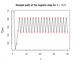
Figure 2: (a) Plot of a sample path associated to the logistic map $T_{\theta}(x)=\theta x(1-x)$ for $\theta=10/3$ starting at $u_{0}=\pi/3.2$ showing an attracting periodic orbit of period 2; (b) sample path of the logistic map for $\theta=4$; (c) Histogram of the sample path in (b).

We will now present an example of a family of dynamical systems which will be used in our application in Section 5. Others examples can be found in the supplementary material. For $s>0$, the Manneville-Pomeau transformation $T_{s}:[0,1]\rightarrow[0,1]$, is given by

$$T_{s}(x)=(x+x^{1+s})(\mathrm{mod}\,1).$$ (5)

For $s\in(0,1)$, there exists an absolutely continuous $T_{s}$-invariant probability measure (Thaler, 1980), which can be seen in Figure 3(c). For $s\geq 1$ there exists an absolutely continuous invariant measure which is only $\sigma$-finite (not a probability measure). Figure 3(a) show the Manneville-Pomeau transformation for $s=0.75$. The Manneville-Pomeau transformation presents a property referred to as transition to turbulence through intermittency (Eckmann, 1981). The Manneville-Pomeau transformation has an indifferent fixed point at $0$ and, hence, it is not uniformly expanding. The chaotic processes associated to $T_{s}$ are often called Manneville-Pomeau processes which present a very slow correlation decay when $s\in(0.5,1)$, characteristic of long range dependent processes and it is commonly viewed as an alternative model for long range dependence outside the classical duet of Fractional Brownian Motion and ARFIMA processes. This slow decay is mainly due to the presence of laminar behavior near zero, which can be seen in Figure 3(b).

   

Figure 3: (a) A plot of the Manneville-Pomeau transformation (5) for $s=0.75$. (b) Sample path of this map for $u_{0}=\pi/4$ showing laminar behavior near zero. (c) Histogram of the first 100,000 iterates of the map.

2.3 General results on the $\beta$ARC model

We will now present some general results about the $\beta$ARC model. Some of them concern the pure $\beta$ARC model, some other involve the presence of the dynamics alongside random covariates (but no AR structure) while others deal with the full $\beta$ARC model. We begin with Proposition 2.1. This result, for the pure $\beta$ARC model, shows that the covariance structure of the dynamics $\{\mu_{t}\}_{t\geq 1}$ ultimately determines the unconditional covariance structure of the process $\{Y_{t}\}_{t\geq 1}$. To the best of our knowledge, similar results are not available for any other competing GARMA-like processes in the literature.

Proposition 2.1.

Let $\{Y_{t}\}_{t\geq 1}$ be a pure $\beta$ARC process following (4). Then, for all $t,h>0$,

1. $\mathds{E}(Y_{t})=\mathds{E}(\mu_{t})$.

2. $\mathrm{Var}(Y_{t})=\mathrm{Var}(\mu_{t})+\dfrac{1}{1+\nu}\mathds{E}\big{(}\mu_{t}(1-\mu_{t})\big{)}$.

3. $\mathrm{Cov}(Y_{t},Y_{t+h})=\mathrm{Cov}(\mu_{t},\mu_{t+h})$.

Proof: Item (a) follows from $\mathds{E}(Y_{t})=\mathds{E}\big{(}\mathds{E}(Y_{t}|\mathscr{F}_{t-1})\big{)}=\mathds{E}(\mu_{t})$, while (b) follows from the identity $\mathrm{Var}(Y_{t})=\mathrm{Var}\big{(}\mathds{E}(Y_{t}|\mathscr{F}_{t-1})\big{)}+\mathds{E}\big{(}\mathrm{Var}(Y_{t}|\mathscr{F}_{t-1})\big{)}$ and (a). As for (c), for any $t,h>0$, from item (a) we obtain

$$\mathrm{Cov}(Y_{t},Y_{t+h})=\mathds{E}(Y_{t}Y_{t+h})-\mathds{E}(Y_{t})\mathds{E}(Y_{t+h})=\mathds{E}(Y_{t}Y_{t+h})-\mathds{E}(\mu_{t})\mathds{E}(\mu_{t+h}).$$ (6)

Now, notice that $\mu_{t}$ is $\mathscr{F}_{1}$-measurable, for all $t>0$, so that

$$\mathds{E}(Y_{t}Y_{t+h}) =\mathds{E}\big{(}\mathds{E}(Y_{t}Y_{t+h}|\mathscr{F}_{t+h-1})\big{)}=\mathds{E}\big{(}Y_{t}\mathds{E}(Y_{t+h}|\mathscr{F}_{t+h-1}))=\mathds{E}(Y_{t}\mu_{t+h})$$

$$=\mathds{E}\big{(}\mathds{E}(Y_{t}\mu_{t+h}|\mathscr{F}_{t-1})\big{)}=\mathds{E}\big{(}\mu_{t+h}\mathds{E}(Y_{t}|\mathscr{F}_{t-1})\big{)}=\mathds{E}(\mu_{t}\mu_{t+h}),$$ (7)

and the result follows upon replacing (2.3) into (6).  

Conditions for stationarity of other dynamical models for time series following a GARMA approach are traditionally very hard to obtain and remain an open subject for most traditional models, such as $\beta$ARMA (Rocha and Cribari-Neto, 2009), $\beta$ARFIMA (Pumi et al., 2019) and KARMA models (Bayer et al., 2017) except under trivial scenarios. In the next result we show that $\beta$ARC models are stationary in a very broad specification and under easily verifiable conditions.

Theorem 2.1.

Let $\{Y_{t}\}_{t\geq 1}$ be a $\beta$ARC model with $\nu>0$ and

$$\eta_{t}=g(\mu_{t})=\alpha+\boldsymbol{x}_{t}^{\prime}\boldsymbol{\beta}+h\big{(}T^{t-1}(U_{0})\big{)},$$

where $\{\boldsymbol{x}_{t}\}_{t\geq 1}$ is a set of random covariates, $g$ and $h$ are twice continuously differentiable, one to one link functions, and $U_{0}$ is a random variable such that $T^{t}(U_{0})\in(0,1)$, for all $t\geq 0$, with probability 1. Then $\{(Y_{t},\mu_{t})\}_{t\geq 1}$ is jointly stationary if and only if $\{\mu_{t}\}_{t\geq 1}$ is stationary.

Proof: Suppose that $\{\mu_{t}\}_{t\geq 1}$ is stationary. For any arbitrary positive integer $k$, let $t_{1},\cdots,t_{k}$ be distinct time points, $\boldsymbol{t}=(t_{1},\cdots,t_{k})$, $\boldsymbol{t}+h=(t_{1}+h,\cdots,t_{k}+h)$, $\boldsymbol{Y_{t}}=(Y_{t_{1}},\cdots,Y_{t_{k}})$ and $\boldsymbol{\mu_{t}}=(\mu_{t_{1}},\cdots,\mu_{t_{k}})$. Using Riemman-Stieltjes integration we have

$$F_{Y_{t}|\mu_{t}}(y|z)=P(Y_{t}\leq y|\mu_{t}=z)=\int_{0}^{y}dF_{Y_{t}|\mu_{t}}(u|z),\quad\forall y,z\in(0,1),$$

$$F_{\boldsymbol{\mu_{t}}}(v_{1},\dots,v_{k})=P(\mu_{t_{1}}\leq v_{1},\dots,\mu_{t_{k}}\leq v_{k})=\int_{0}^{v_{1}}\dots\int_{0}^{v_{k}}dF_{\boldsymbol{\mu_{t}}}(z_{1},\dots,z_{k})$$

and

$$F_{\boldsymbol{Y_{t}},\boldsymbol{\mu_{t}}}(u_{1},\dots,u_{k},v_{1},\dots,v_{k}) =P(Y_{t_{1}}\leq u_{1},\dots,Y_{t_{k}}\leq u_{k},\mu_{t_{1}}\leq v_{1},\dots,\mu_{t_{k}}\leq v_{k})$$

$$=\int_{0}^{u_{1}}\dots\int_{0}^{u_{k}}\int_{0}^{v_{1}}\dots\int_{0}^{v_{k}}dF_{\boldsymbol{Y_{t}},\boldsymbol{\mu_{t}}}(y_{1},\dots,y_{k},z_{1},\dots,z_{k}),$$

for all $u_{1},\dots,u_{k},v_{1},\dots,v_{k}\in(0,1)$, where $dF_{Y_{t},\mu_{t}}$, $dF_{\boldsymbol{\mu_{t}}}$ and $dF_{\boldsymbol{Y_{t}},\boldsymbol{\mu_{t}}}$ are the integrands of the Riemann-Stieltjes integrals. Observe that, for all $t>0$, given $\mu_{t}=z$, the random variable $Y_{t}$ depends, neither on the past information $\{Y_{s},\mu_{s}\}_{s<t}$, nor on the future $\mu_{s}$, $s>t$, so that

$$dF_{\boldsymbol{Y_{t}},\boldsymbol{\mu_{t}}}(y_{1},\dots,y_{k},z_{1},\dots,z_{k})=dF_{\boldsymbol{\mu}_{\boldsymbol{t}}}(z_{1},\dots,z_{k})\prod_{j=1}^{k}dF_{Y_{t_{j}}|\mu_{t_{j}}}(y_{j}|z_{j}).$$

It is easy to see that $dF_{Y_{t}|\mu_{t}}(y|z)=f(y;z,v|\mathscr{F}_{t-1})dy$, where $f$ is the conditional density defined by (2) and that $dF_{Y_{t}|\mu_{t}}(y|z)=dF_{Y_{1}|\mu_{1}}(y|z)=dF_{Y_{t+h}|\mu_{t+h}}(y|z)$, for all $t,h>0$, so that, from the stationarity of $\{\mu_{t}\}_{t\geq 1}$, it follows that, for all $A_{i},B_{i}\subset(0,1)$, $i=1,\dots,k$,

$$P(Y_{t_{1}}\in A_{1},\dots, Y_{t_{k}}\in A_{k},\mu_{t_{1}}\in B_{1},\dots,\mu_{t_{k}}\in B_{k})=$$

$$=\int_{A_{1}}\dots\int_{A_{k}}\int_{B_{1}}\dots\int_{B_{k}}dF_{\boldsymbol{Y_{t}},\boldsymbol{\mu_{t}}}(y_{1},\dots,y_{k},z_{1},\dots,z_{k})$$

$$=\int_{A_{1}}\dots\int_{A_{k}}\int_{B_{1}}\dots\int_{B_{k}}dF_{\boldsymbol{\mu}_{\boldsymbol{t}}}(z_{1},\dots,z_{k})\prod_{j=1}^{k}dF_{Y_{t_{j}}|\mu_{t_{j}}}(y_{j}|z_{j})$$

$$=\int_{A_{1}}\dots\int_{A_{k}}\int_{B_{1}}\dots\int_{B_{k}}dF_{\boldsymbol{\mu}_{\boldsymbol{t}+h}}(z_{1},\dots,z_{k})\prod_{j=1}^{k}dF_{Y_{t_{j}+h}|\mu_{t_{j}+h}}(y_{j}|z_{j})$$

$$=P(Y_{t_{1}+h}\in A_{1},\dots,Y_{t_{k}+h}\in A_{k},\mu_{t_{1}+h}\in B_{1},\dots,\mu_{t_{k}+h}\in B_{k}).$$

This implies that $\{(Y_{t},\mu_{t})\}_{t\geq 1}$ is jointly stationary. The converse is obvious.  

Corollary 2.1.

Under the conditions of Theorem 2.1, if $\{\mu_{t}\}_{t\geq 1}$ is stationary, then so is $\{Y_{t}\}_{t\geq 1}$.

Proof: Observe that, if $\{\mu_{t}\}_{t\geq 1}$ is stationarity then from Theorem 2.1 $\{(Y_{t},\mu_{t})\}_{t\geq 1}$ is jointly stationary and hence, $\{Y_{t}\}_{t\geq 1}$ is stationary.  

Corollary 2.2.

Let $T_{\boldsymbol{\theta}}$ be a dynamical system with ACIM given by $\lambda_{T}$ and let $\{Y_{t}\}_{t\geq 1}$ be a pure chaotic $\beta$ARC model with $\nu>0$ where $\mu_{t}=T_{\boldsymbol{\theta}}^{t-1}(U_{0})$ and $U_{0}$ is chosen accordingly to $\lambda_{T}$. Then $\{Y_{t}\}_{t\geq 1}$ is stationary and the common marginal distribution $F_{Y_{t}}$ is absolutely continuous with respect to the Lebesgue measure, with unconditional density given by

$$f_{Y_{t}}(y)=\int_{0}^{1}f_{Y_{t}|\mu_{t}}(y|z)\lambda_{T}(dz),$$

where $f_{Y_{t}|\mu_{t}}(y|z)=f(y;z,\nu|\mathscr{F}_{t-1})$ is the conditional density of $Y_{t}$ given $\mu_{t}$, defined by (2).

Proof: The stationarity of $\{Y_{t}\}_{t\geq 1}$ follows immediately from Corollary 2.1, as $\mu_{t}$ is clearly stationary in this case. Now, let $f_{Y_{t},\mu_{t}}$ denote the joint density of $\big{(}Y_{t},\mu_{t}\big{)}$, so we have

$$f_{Y_{t}}(y)=\int_{0}^{1}f_{Y_{t},\mu_{t}}(y,z)dz=\int_{0}^{1}f_{Y_{t}|\mu_{t}}(y|z)\lambda_{T}(dz),$$

and the proof is complete  .

Corollary 2.3.

Let $T_{\boldsymbol{\theta}}$ be a dynamical system with ACIM given by $\lambda_{T}$, and let $\{\boldsymbol{x}_{t}\}_{t\geq 1}$ be a set of random covariates. Suppose $\{Y_{t}\}_{t\geq 1}$ is a $\beta$ARC model with $\nu>0$ where

$$\eta_{t}=g(\mu_{t})=\alpha+\boldsymbol{x}_{t}^{\prime}\boldsymbol{\beta}+h\big{(}T^{t-1}(U_{0})\big{)},$$

for two twice continuously differentiable, one to one link functions $g$ and $h$. Suppose $U_{0}$ is chosen according to $\lambda_{T}$. Then if $\{\boldsymbol{x}_{t}\}_{t\geq 1}$ is stationary, so is $\{Y_{t}\}_{t\geq 1}$.

Proof: Since $g$ and $h$ are both measurable functions, $\{\mu_{t}\}_{t\geq 1}$ is stationary if and only if $\{\boldsymbol{x}_{t}\}_{t\geq 1}$ is stationary and the result follows immediately from Theorem 2.1.  

Remark 2.2.

The proof of Theorem 2.1 is also valid under the full specification (3). However, verification of the hypothesis under (3) is difficult since it is not presented in an autoregressive fashion as we write $\eta_{t}$ in terms of past values of $Y_{t}$ and $\boldsymbol{x}_{t}$, which depends on the past of $\eta_{t}$ in a non-trivial way. In this scenario it is challenging to obtain stationarity conditions for $\{\eta_{t}\}_{t\geq 1}$ under the full specification (3). This and the recursive nature of $\mu_{t}$ for similar GARMA-like models, such as the $\beta$ARMA, $\beta$ARFIMA and KARMA, make obtaining stationarity conditions a non-trivial problem for these models.

Before moving on, let us analyze an example that will motivate the next result. We shall analyze the stationarity of the $\beta$ARC model with $T_{k}(x)=(kx)\mathrm{mod}(1)$ for an integer $k>0$. In this case, the Lebesgue measure in $[0,1]$ is $T_{k}$ invariant and the unconditional distribution of $Y_{t}$ is given by

$$f_{Y_{t}}(x)=\frac{\Gamma(\nu)(1-x)^{\nu-1}}{x}\int_{0}^{1}\left[\frac{x}{1-x}\right]^{\nu z}\frac{1}{\Gamma(\nu z)\Gamma\big{(}\nu(1-z)\big{)}}dz.$$

The behavior of $f_{Y_{t}}$ depends on the magnitude of $\nu$. In Figure 4 we show the behavior for several values of $\nu$.

     

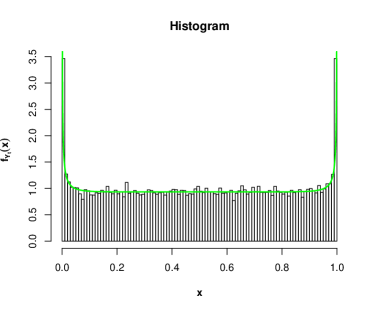
Figure 4: (a) The unconditional density of the pure $\beta$ARC model with $T_{k}(x)=(kx)\mathrm{mod}(1)$ and (b) histogram of an associated sample of size $n=30,000$ starting at $u_{0}=\pi/4$, with $\nu=15$ and $k=3$, showing the associated unconditional density (green).

Let

$$T_{\theta}(x)=\begin{cases}\frac{x}{\theta}&\mbox{if}\;\;0\leq x<\theta,\\ \frac{\theta(x-\theta)}{1-\theta}&\mbox{if}\;\;\theta\leq x\leq 1.\end{cases}$$ (8)

More details regarding this map can be found in the Supplementary material (Map 2). Now consider the pure $\beta$ARC model coupled with (8). For any $\theta\in(0,1)$, the unconditional distribution of $Y_{t}$ is given by

$$f_{Y_{t}}(x)=\frac{\Gamma(\nu)(1-x)^{\nu-1}}{x}\bigg{(}\int_{0}^{x}\left[\frac{x}{1-x}\right]^{\nu z} \frac{1}{(2-z)\Gamma(\nu z)\Gamma\big{(}\nu(1-z)\big{)}}dz+$$

$$+ \int_{x}^{1}\left[\frac{x}{1-x}\right]^{\nu z}\frac{1}{z(2-z)\Gamma(\nu z)\Gamma\big{(}\nu(1-z)\big{)}}dz\bigg{)}.$$

In Figure 5 we show the behavior of $f_{Y_{t}}$ for several values of $\nu$.

     

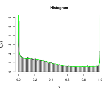
Figure 5: (a) The unconditional density of the pure $\beta$ARC model for (8) and (b) histogram of an associated sample of size $n=30,000$ starting at $u_{0}=\pi/4$, with $\nu=15$ and $\theta=0.4$ showing the associated unconditional density (green).

The next result shows, as the last example suggests, that the larger the precision parameter is, the closer the $\beta$ARC model resembles its conditional mean. Observe that the result does not require stationarity to hold.

Theorem 2.2.

Let $\{Y_{t}\}_{t\geq 1}$ be a $\beta$ARC process. Then, for each fixed $t>0$,

$$Y_{t}\overset{d}{{\longrightarrow}}\mu_{t},\quad\mbox{as }\nu\to\infty.$$

Proof: First, for fixed $t>0$, observe that $\mathrm{Var}(Y_{t}|\mathscr{F}_{t-1})=\frac{\mu_{t}(1-\mu_{t})}{1+\nu}\rightarrow 0$ as $\nu\to\infty$. Now we can also use the fact that $\mathds{E}(Y_{t}|\mathscr{F}_{t-1})=\mu_{t}$ and Chebysheff’s inequality to conclude that $Y_{t}$ conditionally converges in probability to $\mu_{t}$, which implies convergence in distribution. Therefore, for any $0<c<1$ which is a continuity point of $F_{\mu_{t}}$, we have

$$P(Y_{t}\leq c|\mu_{t}=z)\longrightarrow\begin{cases}1\mbox{ if }c>z,\\ 0\mbox{ if }c<z,\end{cases}$$

when $\nu\to\infty$, which implies

$$P(Y_{t}\leq c)=\int_{0}^{1}P(Y_{t}\leq c|\mu_{t}=z)dF_{\mu_{t}}(z)\rightarrow\int_{0}^{c}1\,dF_{\mu_{t}}(z)=P(\mu_{t}\leq c)$$

when $\nu\to\infty$, by the Lebesgue dominated convergence theorem.  

In the case of the pure $\beta$ARC model, if the map $T_{\boldsymbol{\theta}}$ has an ACIM $\lambda_{T}$ and $U_{0}$ is distributed according to $\lambda_{T}$, the distribution of $\mu_{t}$ is given by $\lambda_{T}$. Therefore, Theorem 2.2 and Birkhoff’s Theorem suggests that the histogram is a valuable tool in choosing the family of maps $T_{\boldsymbol{\theta}}$ to be used to model a given time series.

The next theorem presents a simple condition under which the strong law of large numbers holds for $\beta$ARC process. In particular, for a stationary $\beta$ARC process, the strong law of large numbers for $\{Y_{t}\}_{t\geq 1}$ is related to the covariance structure of the dynamical system $\{\mu_{t}\}_{t\geq 1}$.

Theorem 2.3.

Let $\{Y_{t}\}_{t\geq 1}$ be a $\beta$ARC process and $\varphi:[0,1]\to\mathds{R}$ be a measurable function such that $\mathds{E}(\varphi(Y_{t})^{2})<\infty$, for all $t>0$. If

$$\sum_{k=1}^{\infty}\frac{\sup_{t\geq 1}\Big{\{}\big{|}\mathrm{Cov}\big{(}\varphi(Y_{t}),\varphi(Y_{t+k})\big{)}\big{|}\Big{\}}}{k^{q}}<\infty,\quad\mbox{for some $0\leq q<1$},$$ (9)

and

$$\sum_{k=1}^{\infty}\frac{\mathrm{Var}\big{(}\varphi(Y_{k})\big{)}\ln(k)^{2}}{k^{2}}<\infty$$ (10)

then

$$\lim_{n\to\infty}\frac{1}{n}\sum_{\ell=0}^{n-1}\big{[}\varphi(Y_{\ell})-\mathds{E}\big{(}\varphi(Y_{\ell})\big{)}\big{]}=0,\quad\mbox{a.s.}$$ (11)

Proof: Observe that, conditions (9) and (10) translate into conditions (3.2) and (3.1) in theorem 1 in Hu et al. (2008), respectively. Hence, the result in the mentioned theorem hold which translates into (11).  

Remark 2.3.

Observe that if $\{Y_{t}\}_{t\geq 1}$ is stationary, so is $\{\varphi(Y_{t})\}_{t>0}$, hence (10) is always satisfied and condition (9) becomes

$$\sum_{k=1}^{\infty}\frac{\big{|}\mathrm{Cov}\big{(}\varphi(Y_{t}),\varphi(Y_{t+k})\big{)}\big{|}}{k^{q}}<\infty,\quad\mbox{for some $0\leq q<1$}.$$

Moreover, in this case the conclusion is a Birkhoff-type theorem since (11) becomes

$$\lim_{n\to\infty}\frac{1}{n}\sum_{\ell=0}^{n-1}\varphi(Y_{\ell})=\int\varphi(z)dF_{Y_{t}}(z)\quad\mbox{a.s.}$$

Remark 2.4.

An interesting corollary to Theorem 2.3 is obtained by taking $\varphi$ as the identity function. In view of Proposition 2.1 and Corollary 2.1, for a pure $\beta$ARC associated to a dynamical system presenting ACIM $\lambda_{T}$, with $U_{0}\sim\lambda_{T}$, a sufficient condition for (9) to hold is

$$\sum_{k=1}^{\infty}\frac{|\mathrm{Cov}(\mu_{t},\mu_{t+k})|}{k^{q}}<\infty,\quad\mbox{for some $0\leq q<1$}.$$ (12)

This result is very convenient since a vast literature concerning the covariance structure of dynamical systems is available. For instance, it is well known that if the dynamical system is hyperbolic, then the covariance decays exponentially fast (see Baladi, 2000; Hasselblatt and Katok, 1996) and the condition (12) holds for all $q\in[0,1)$. Furthermore, if the system presents long range dependence in the sense that $\mathrm{Cov}(\mu_{t},\mu_{t+k})\sim L(k)k^{-b}$, for $0<b<1$, for some slowly varying function $L$, then condition (12) holds, for all $1-b<q<1$. This is the case, for instance, for the Manneville-Pomeau map (Map 4) when $s\in(0.5,1)$. Finally, in this context, (12) is a sufficient condition for a strong law of large number for $Y_{t}$ to hold.

3 Partial Maximum Likelihood Inference

Parameter inference in the proposed model can be done via partial maximum likelihood estimation (PMLE). Let $\{(y_{t},\boldsymbol{x}_{t}^{\prime})^{\prime}\}_{t=1}^{n}$ be a sample from a $\beta$ARC$(p)$ model following (2) and (3) for a given transformation $T_{\boldsymbol{\theta}}$ depending on an identifiable vector of parameters $\boldsymbol{\theta}=(\theta_{1},\cdots,\theta_{r})^{\prime}\in\Omega_{T}\subseteq\mathds{R}^{r}$ and $h$ a suitable link function. We shall assume that $u_{0}\in(0,1)$ is known and such that $T^{t}(u_{0})\notin\{0,1\}$ for all $t$. Let $\boldsymbol{\gamma}:=(\nu,\alpha,\boldsymbol{\beta}^{\prime},\boldsymbol{\phi}^{\prime},\boldsymbol{\theta}^{\prime})^{\prime}\in\Omega\subseteq(0,\infty)\times\mathds{R}^{p+l+1}\times\Omega_{T}$ be the $(l+p+r+2)$-dimensional vector of parameter related to the model, where $\Omega$ denotes the parameter space. Upon writing

$$\ell_{t}(\boldsymbol{\gamma})=\log\big{(}f(y_{t};\boldsymbol{\gamma}|\mathscr{F}_{t-1})\big{)}=\log\big{(} \Gamma(\nu)\big{)}-\log\big{(}\Gamma(\mu_{t}\nu)\big{)}-\log\big{(}\Gamma\big{(}\nu(1-\mu_{t})\big{)}\big{)}+$$

$$+(\mu_{t}\nu-1)\log(y_{t})+\big{(}\nu(1-\mu_{t})-1\big{)}\log(1-y_{t}),$$

the log-likelihood associated to model (2) and (3) is given by

$$\ell(\boldsymbol{\gamma}):=\sum_{t=1}^{n}\ell_{t}(\boldsymbol{\gamma}).$$

The partial maximum likelihood estimator is then defined as

$$\widehat{\boldsymbol{\gamma}}=\underset{\boldsymbol{\gamma}\in\Omega}{\mathrm{argmax}}\big{\{}\ell(\boldsymbol{\gamma})\big{\}}.$$ (13)

To obtain the PMLE we need to solve the optimization problem (13), which can be done upon finding the score function and solving a non-linear system, by using, for instance, the BFGS optimization algorithm. Alternatively, the optimization problem can also be solved by using other methods such as Nelder-Mead.

Since $\eta_{t}$ is generally a non-linear function of $\boldsymbol{\theta}$, the asymptotic theory of the PMLE in the context of $\beta$ARC models requires some non-trivial adaptations of the existing theory for GARMA-like models (presented, for instance, in Fokianos and Kedem, 2004). A rigorous large sample theory for the PMLE in the context of $\beta$ARC models is subject of a future paper. In the next section (and in the supplementary material accompanying the paper), we shall study the finite sample performance of the PMLE in the context of $\beta$ARC models.

4 Monte Carlo Simulation

In this section we present a short Monte Carlo simulation study to analyze the finite sample performance of the PMLE in the context of $\beta$ARC models. For the sake of brevity, we shall only consider a single scenario. A more extensive Monte Carlo simulation study considering several different scenarios is presented in the Supplementary material accompanying this paper.

We consider parameter estimation via PMLE for a pure chaotic $\beta$ARC model with map $T_{k}(x)=(kx)(\mathrm{mod}\,1)$ for $k\in\{3,5,7\}$, considered known, and three different starting points $u_{0}\in\{0.2+\pi/100,0.5+\pi/100,0.8+\pi/100\}$. We present the results for $\nu=40$ (other cases are presented in the supplementary material). We generate samples $\{y_{t}\}_{t=1}^{n}$ for $n\in\{100,500,1000\}$ by setting

$$\mu_{t}:=T_{k}^{t-1}(u_{0})\quad\mbox{and}\quad y_{t}\sim\mbox{Beta}\big{(}\nu\mu_{t},\nu(1-\mu_{t})\big{)}$$

For all scenarios we perform $1,000$ replications. To obtain the PMLE we solve the optimization problem (13). The maximization of the objective function was performed by considering the so-called Nelder-Mead algorithm implemented in Fortran by Alan Miller and adapted by the authors to handle parameter constraints using the ideas implemented in the matlab function fminsearchbnd. To start the optimization algorithm we calculate the likelihood function for $\nu\in\{5,50,100\}$ and select the one with higher likelihood value as starting point.

All computer codes were written by the authors. The most demanding task of parameter estimation was implemented in FORTRAN, while the other tasks were implemented in R (R Core Team, 2018) version 3.6.1. The necessary shared libraries were also compiled in R version 3.6.1.

Results

Table 1 presents the simulation results. Highlighted in blue and red are the best and worst scenarios in each case, respectively. We observe that as $n$ increases, the bias and standard deviation of the estimated values decrease. From the results we found no relation between $u_{0}$ and $k$ with the estimated value of $\nu$. Figure 6 presents the histograms and boxplots of the results for $u_{0}=0.5+\pi/100$ (the other cases are analogous and can be found in the supplementary material). The histograms suggests that the PMLE in the context of $\beta$ARC models satisfy a central limit theorem. Indeed, applying a Shapiro-Wilk test to the results presented in the top left plot ($k=3$), for $n$ equals 100, 500 and 1,000 the test yields p-values equal to $0.0000$, 0.1077 and 0.2744, respectively.

Table 1: Simulation Results for parameter $\nu$ considering the map $T_{k}(x)=(kx)(\mathrm{mod}\,1)$ with $k\in\{3,5,7\}$ and sample size $n\in\{100,500,1000\}$: the mean estimated value of $\nu$ over 1,000 replications ($\bar{\nu}$), for $\nu=40$, the standard deviation of the estimates ($sd_{\nu}$) and the mean absolute percentage error (MAPE).

	$n=100$			$n=500$			$n=1,000$
$u_{0}$	$\bar{\nu}$	$sd_{\nu}$	MAPE	$\bar{\nu}$	$sd_{\nu}$	MAPE	$\bar{\nu}$	$sd_{\nu}$	MAPE
$k=3$
$0.2+\frac{\pi}{100}$	40.78	5.4388	10.75	40.18	2.3437	4.73	40.14	1.6885	3.42
$0.5+\frac{\pi}{100}$	40.92	5.6838	11.19	40.23	2.3867	4.78	40.15	1.7157	3.46
$0.8+\frac{\pi}{100}$	40.76	5.5986	11.00	40.30	2.4250	4.90	40.19	1.6813	3.40
$k=5$
$0.2+\frac{\pi}{100}$	40.78	5.5718	10.89	40.47	2.3862	4.83	40.37	1.6937	3.51
$0.5+\frac{\pi}{100}$	40.72	5.6021	10.94	40.18	2.3819	4.77	40.24	1.7350	3.52
$0.8+\frac{\pi}{100}$	40.94	5.4653	10.86	40.18	2.3451	4.64	40.17	1.6912	3.35
$k=7$
$0.2+\frac{\pi}{100}$	40.99	5.6991	11.31	40.24	2.3998	4.78	40.16	1.7052	3.46
$0.5+\frac{\pi}{100}$	40.64	5.5486	11.06	40.23	2.3665	4.77	40.21	1.7173	3.44
$0.8+\frac{\pi}{100}$	40.82	5.4884	10.95	40.20	2.3940	4.78	40.15	1.7040	3.39

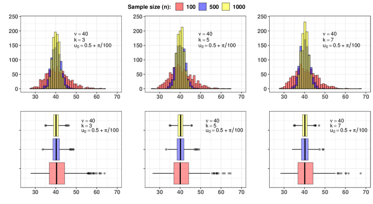
Figure 6: Boxplots of the estimated values, from 1,000 replications, for the parameter $\nu=40$ considering the map $T_{k}(x)=(kx)(\mathrm{mod}\,1)$ with $k\in\{3,5,7\}$, $n\in\{100,500,1000\}$ and starting points $u_{0}\in\{0.2+\pi/100,0.5+\pi/100,0.8+\pi/100\}$.

5 Real data Application

In this section we illustrate the usefulness of the $\beta$ARC model in modeling real data. The variable of interest is the proportion of stocked hydroelectric energy in South Brazil. The data are monthly averages from January 2001 to April 2017 and can be freely downloaded from ONS’s (the Brazilian national operator of the electrical system) website ( http://www.ons.org.br). For comparison with other models, 6 months of data, from November 2016 to April 2017, were reserved for out-of-sample forecasting, yielding a sample of size $n=190$ for fitting purposes. This data was first considered in Scher et al. (2019) where the authors fit a $\beta$ARMA(1,1) model to the data and compare its forecasting capabilities with 4 other models: the KARMA(1,1) of Bayer et al. (2017), Gaussian ARMA(1,1) and AR(2) models and also with the Holt exponential smoothing algorithm. Our goal is to fit the proposed $\beta$ARC model models and compare to the results reported in Scher et al. (2019).

Figure 7 brings the time series plot of the data. In order to fit a $\beta$ARC model, we apply the Manneville-Pomeau transformation (5) with $h$ as the identity link. For $g$ in $\eta_{t}$ we take the cloglog link given by $g(x)=\log(-\log(1-x))$. To obtain the PMLE estimates based on the log-likelihood we first employ a L-BFGS-B optimization with numerical derivatives and then a Nelder-Mead optimization algorithm starting at the values obtained from the L-BFGS-B. This approach showed better results in practice. As for the $p$-values, they are obtained from Wald’s $z$ test, based on the numerical hessian (a rigorous asymptotic theory for the PMLE in the context of $\beta$ARC model is under development and shall be presented in another paper).

One delicate computational problem is defining which $u_{0}$ to apply. Observe that although $s$ is identifiable, $u_{0}$ is not as the Manneville-Pomeau transformation presents two full branches. However, the sample path of the transformation is identifiable (except for $u_{0}$), hence, the specific value of $u_{0}$ brings no useful information in practice, but it is needed to start the PMLE. We overcome this problem with a simple strategy: optimization was performed based on a grid of 900 initial points for $u_{0}$ starting at $\pi/1000$ and ending on $1-\pi/1000$. The whole process takes less than 2 minutes in any average computer running Windows 10.

For model selection, we consider only models for which all the coefficients were significant and that the residuals (defined as $y_{t}-\mu_{t}$) did not present any serial correlation, condition tested using the Ljung-Box test considering $m=20$ lags. Among all models satisfying these conditions, we chose the one with the smallest in-sample mean absolute prediction error (MAPE-IN), which we shall call Model 1, and also the one with the highest likelihood (Model 2). Under both metrics, a simple $\beta$ARC(1) model satisfied the aforementioned conditions.

Table 2 presents the fitted $\beta$ARC(1) models while Table 3 presents the corresponding in-sample and out-of-sample accuracy measures. Presented are the mean absolute percentage error (MAPE), the mean percentage error (MPE), the average error (ME), the mean absolute error (MAE) and root mean square error (RMSE) for the in-sample and out-of-sample results. We observe that Model 2, obtained via likelihood, presents borderline better in sample accuracy measures than Model 1, except for the MAPE. In terms of out-of sample performance, however, Model 2 outperforms Model 1 in all measures by a large margin. In Figure 8(b) and (c), we present the observed time series along with in-sample and out-of-sample forecast for models 1 and 2.

Figure 7: Time series plot of the proportion of stocked energy, showing the data used to fit the model (black) and the reserved data (blue).

Table 2: Fitted $\beta$ARC(1) models for the stocked energy data.

Model 1: smallest MAPE-IN			Model 2: highest likelihood
	Estimate	$p$-value		Estimate	$p$-value
$\alpha$	-0.3170	0.0000	$\alpha$	-0.3653	0.0000
$\phi_{1}$	0.7634	0.0000	$\phi_{1}$	0.7107	0.0000
$s$	0.8165	–	$s$	0.3706	–
$\nu$	6.3634	–	$\nu$	10.5798	–
$u_{0}=0.810052910479796$			$u_{0}=0.423177621111067$
Log-likelihood: $120.01$			Log-likelihood: $134.70$
AIC: $-232.03$   BIC: $-219.04$			AIC: $-261.40$   BIC: $-248.41$

Table 3: In and out-of-sample forecasting measures for the two fitted $\beta$ARC(1) models presented in Table 2. (M1 and M2 here stand for Model 1 and Model 2.)

	In-sample accuracy measures					Out-of-sample accuracy measures
	MAPE	MPE	ME	MAE	RMSE	MAPE	MPE	ME	MAE	RMSE
M1	14.16%	2.34%	0.0337	0.0957	0.1291	4.92%	3.40%	0.0177	0.0277	0.0372
M2	14.67%	-1.89%	0.0069	0.0937	0.1217	28.63%	-28.63%	-0.1620	0.1620	0.1801

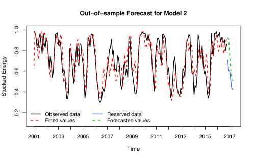
Figure 8: The observed time series and the in-sample and out-of-sample forecasted values for the fitted $\beta$ARC models 1 (a) and 2 (b).

As mentioned before, Scher et al. (2019) also considered the same data and modeled it using 5 different models ($\beta$ARMA(1,1), KARMA(1,1), Gaussian ARMA(1,1), Gaussian AR(2) models and the Holt exponential smoothing algorithm). Among these models, the authors report that the $\beta$ARMA(1,1) presented the smallest AIC (-307.9635) and also the best out-of-sample forecasting performance with an MAE of 0.1839 for the same data considered here (other forecasting accuracy measures were not reported). We observe that both fitted $\beta$ARC(1) outperform the fitted $\beta$ARMA(1,1) model in terms of out-of sample performance. Model 1, in special, present out-of-sample MAE of only 0.0277, considerably smaller than the $\beta$ARMA’s MAE.

6 Conclusion

Here we introduced the Beta Autoregressive Chaotic ($\beta$ARC) processes, a class of dynamic models for time series taking values on the unit interval. The model follows similar structure of other GARMA-like models (in the sense of Benjamin et al., 2003). The random component of the process was modeled through a beta distribution, conditioned on the past information, while the conditional mean was specified allowing the presence of covariates (random and/or deterministic) and an extra additive term defined by the iteration of a map $T$ defined on $[0,1]$, inspired on the theory of chaotic processes and dynamical systems. This additive term is able to model a wide variety of behaviors in the processes’ conditional mean, including short and long range dependence, attracting and/or repelling fixed or periodic points, presence or absence of absolutely continuous invariant measure, among others, allowing for a much broader and flexible dependence structure compared to competitive GARMA-type models presented in the literature.

In the $\beta$ARC model, the extra additive term’s definition borrows ideas from dynamical systems. For this reason, a review on the main definitions concerning one dimensional dynamical systems was presented in order to describe the wide variety of behaviors that $T$ can present. Among the main features of the underlying transformation we focused on the existence of attracting and/or repelling fixed or periodic points and the presence or absence of absolutely continuous invariant measure. We also discussed how the characteristics of the chaotic process are reflected into the observed time series. In particular, we showed that, as the precision parameter $\nu$ increases, the closer the sample path resembles the conditional mean’s dynamics. We also presented some examples where the systematic component can accommodate short or long range dependence, periodic behavior and/or laminar phases.

We also presented some theoretical results which are new in the literature in the sense that are not known for any other GARMA-like process. For instance, we derived the covariance structure of the $\beta$ARC models and obtained sufficient conditions for stationarity, law of large numbers and a Birkhoff-type result to hold. In particular, we showed that, in the absence of an autoregressive component, if $T$ has an absolute continuous $T$-invariant measure and the covariate process is stationary, then the $\beta$ARC processes is stationary.

A short Monte Carlo simulation study to assess the finite sample performance of the PMLE in the context of pure chaotic $\beta$ARC models was presented. The simulation results show small bias and standard deviations which, as expected, decrease as $n$ increases. Histograms of the simulated results also suggest that the PMLE is asymptotically normally distributed in the context of the simulation. A much broader Monte Carlo simulation study is presented in the supplementary material that accompanies the paper.

Finally, an application of the proposed methodology to real data was presented. The variable of interest is the proportion of stored hydroelectrical energy in Southern Brazil from January 2001 through October 2016. Overall the model was capable of fitting the data very well, outperforming competing standard methods in terms of out-of-sample forecasting accuracy.

Acknowledgments

T.S. Prass gratefully acknowledges the support of FAPERGS (ARD 01/2017, Processo 17/2551-0000826-0).

See pages - of supplementary.pdf

References

- Baladi (2000) Baladi, V. (2000) Positive Transfer Operators and Decay of Correlations. World Scientific.
- Bayer et al. (2017) Bayer, F. M., Bayer, D. M. and Pumi, G. (2017) Kumaraswamy autoregressive moving average models for double bounded environmental data. Journal of Hydrology, 555, 385–396.
- Benjamin et al. (2003) Benjamin, M. A., Rigby, R. A. and Stasinopoulos, D. M. (2003) Generalized autoregressive moving average models. Journal of the American Statistical Association, 98, 214–223.
- Box et al. (2008) Box, G., Jenkins, G. M. and Reinsel, G. (2008) Time series analysis: forecasting and control. Hardcover, John Wiley & Sons.
- Boyarsky and Gora (1997) Boyarsky, A. and Gora, P. (1997) Laws of Chaos. Birkhauser.
- Brockwell and Davis (1991) Brockwell, P. J. and Davis, R. A. (1991) Time Series: Theory and Methods. Springer-Verlag, 2 edn.
- Ding and Zhou (2009) Ding, J. and Zhou, A. (2009) Statistical properties of deterministic systems. Springer Science & Business Media.
- Eckmann (1981) Eckmann, J. P. (1981) Roads to turbulence in dissipative dynamical systems. Rev. Mod. Phys., 53, 643–654.
- Ferrari and Cribari-Neto (2004) Ferrari, S. L. P. and Cribari-Neto, F. (2004) Beta regression for modelling rates and proportions. Journal of Applied Statistics, 31, 799–815.
- Fokianos and Kedem (2004) Fokianos, K. and Kedem, B. (2004) Partial likelihood inference for time series following generalized linear models. Journal of Time Series Analysis, 25, 173–197.
- Gandolfo (2009) Gandolfo, G. (2009) Economic Dynamic. Springer.
- Hasselblatt and Katok (1996) Hasselblatt, B. and Katok, A. (1996) Introduction to the Modern Theory of Dynamical Systems. Cambridge University Press.
- Honsking (1981) Honsking, J. R. M. (1981) Fractional differencing. Biometrika, 1, 165–176.
- Hu et al. (2008) Hu, T.-C., Rosalsky, A. and Volodin, A. (2008) On convergence properties of sums of dependent random variables under second moment and covariance restrictions. Statistics & Probability Letters, 78, 1999 – 2005.
- Jackson and Radunskaya (2015) Jackson, T. and Radunskaya, A. (2015) Applications of Dynamical Systems in Biology and Medicine. Springer.
- Lasota and Yorke (1973) Lasota, A. and Yorke, J. A. (1973) On the existence of invariant measures for piecewise monotonic transformations. Transactions of the American Mathematical Society, 186, 481–488.
- de Melo and Van Strien (1993) de Melo, W. and Van Strien, S. (1993) One-Dimensional Dynamics. Springer-Verlag.
- Palma (2007) Palma, W. (2007) Long-Memory Time Series: Theory and Methods. Wiley Series in Probability and Statistics. Wiley.
- Pumi et al. (2019) Pumi, G., Valk, M., Bisognin, C., Bayer, F. M. and Prass, T. S. (2019) Beta autoregressive fractionally integrated moving average models. Journal of Statistical Planning and Inference, 200, 196–212.
- R Core Team (2018) R Core Team (2018) R: A Language and Environment for Statistical Computing. R Foundation for Statistical Computing, Vienna, Austria. URL: https://www.R-project.org/.
- Rocha and Cribari-Neto (2009) Rocha, A. V. and Cribari-Neto, F. (2009) Beta autoregressive moving average models. Test, 18, 529–545.
- Scher et al. (2019) Scher, V. T., Cribari-Neto, F., Pumi, G. and Bayer, F. M. (2019) Goodness-of-fit tests for ARMA hydrological time series modeling. Environmetrics. Accepted for publication.
- Thaler (1980) Thaler, M. (1980) Estimates of the invariant densities of endomorphisms with indifferent fixed points. Israel Journal of Mathematics, 37, 303–314.
- Zebrowsky (2001) Zebrowsky, J. J. (2001) Intermittency in human heart rate variability. Acta Physica Polonica B, 32, 1531–1540.
- Zeger and Qaqish (1988) Zeger, S. L. and Qaqish, B. (1988) Markov regression models for time series: a quasi-likelihood approach. Biometrics, 44, 1019–1031.