Utility-driven Data Analytics on Uncertain Data

Abstract

Modern Internet of Things (IoT) applications generate massive amounts of data, much of it in the form of objects/items of readings, events, and log entries. Specifically, most of the objects in these IoT data contain rich embedded information (e.g., frequency and uncertainty) and different levels of importance (e.g., unit utility of items, interestingness, cost, risk, or weight). Many existing approaches in data mining and analytics have limitations such as only the binary attribute is considered within a transaction, as well as all the objects/items having equal weights or importance. To solve these drawbacks, a novel utility-driven data analytics algorithm named HUPNU is presented, to extract High-Utility patterns by considering both Positive and Negative unit utilities from Uncertain data. The qualified high-utility patterns can be effectively discovered for risk prediction, manufacturing management, decision-making, among others. By using the developed vertical Probability-Utility list with the Positive-and-Negative utilities (PU^±-list) structure, as well as several effective pruning strategies. Experiments showed that the developed HUPNU approach performed great in mining the qualified patterns efficiently and effectively.

I Introduction

With the increasing prevalence of sensors, mobile phones, actuators, and RFID tags, Internet of Things (IoT) applications generate massive amounts of rich data per day [1, 2, 3]. Examples include the control signals issued to Internet-connected devices like lights or thermostats, measurements from industrial and medical equipment, manufacturing data, or log files from smart-phones that record the complex behavior of sensor-based applications. These applications need to find frequent patterns that represent typical system behavior (e.g., [2, 4, 5]) as well as high risk/utility patterns that represent very important knowledge from normal behavior [6, 7, 8]. For industrial areas [3, 9], various algorithms have been designed by applying data mining methods [3, 10]. These methods can be used to evaluate the complicated and complex data from the industry and solve existing problems.

In some industrial areas, manufacturing schedules can be planned by the discovered information and knowledge, which can then be used to increase and gain utilities, maximally [3, 11]. Pattern mining and analysis, from an industrial research perspective, provides a unique and up-to-date insight into the manufacturing industry [3]. There are many industrial utility-driven manufacturing systems with different IoT applications. Consider an environment with all types of sensors to monitor abnormal conditions. Let each transaction denote the set of sensors showing above normal value at a particular instance, and the value associated with each sensor can be the abnormality or risk measure. Here the number of units can mean the number of abnormal sensors of the same type, then how to discover the high risk patterns is quite useful for manufacturing analytics in Internet of Things. In the retail industry, it can identify the purchase behaviors of customers, which can be used to make specific decisions and improve the service quality of customers. However, existing Frequent-based Pattern Mining (FPM) algorithms [10] ignore that information, and the discovered information or pattern may contain useless knowledge, such as items with a lower utility that may be discovered. Thus, traditional FPM cannot handle the problem of the quantitative databases, and also fails to extract the utility-driven patterns which are insightful for data analytics. A new utility-driven data analytics framework named High-Utility Pattern Mining (HUPM) [6, 7, 8] was presented to provide a solution to the above limitations. It is important to notice that the utility concept can be referenced to reflect multiple participants’ satisfaction [12], utility [11, 13], revenue [14], risk [13], or weight [15].

I-A Motivation

To reveal high utility/risk patterns for decision-making, it considers the quantitative database, as well as the unit utility of the items. The analytics of using HUPM instead of FPM is quite helpful for system monitoring, planning, manufacturing management, and decision-making [2, 3, 11]. Most algorithms in traditional HUPM consider all items to have positive unit utilities/risks. When the items have the constraint of negative values, for example sales discount (e.g., buy two get one free) or if a supermarket/retail store sells the products at a loss to stimulate the sales of other relative items (e.g., sell printers to promote the notebook/PC), traditional HUPM cannot mine meaningful information. This situation happens in real-life scenarios, especially when promoting some profitable items for gaining more money in cross-selling conditions. Some prior works have mentioned that traditional HUPM algorithms [6, 8] may generate incomplete and missing information [16] when the dataset consists of negative unit utility objects/items.

For analyzing the complex industrial data and manufacturing data [2, 11, 17], it may encounter various challenges, i.e., the embedded uncertainty, positive risk and negative risk, and other factors. The uncertainty factor exists in many realistic situations, such as the collection of noisy data sources (e.g., GPS, wireless sensor network, RFID, or WiFi systems) [18, 19]. Traditional pattern mining algorithms cannot be utilized straightforwardly to inaccurate or uncertain environments for mining the required knowledge or information. The reason for this is that the utility can be considered as a semantic measure to value how the “utility” of a pattern based on users’ priori experience, goal, and knowledge, and the uncertainty can be considered as an objective measure to value the probability of a pattern as an objective existence; they are two totally different factors. Most existing utility-based algorithms have been studied to handle precise data, while they are unable to deal with data uncertainty [20]. If the uncertain factor was not considered in the mining process, it may find useless or misleading information with low existential probability.

I-B Contribution

To solve the above limitations and problems, we attempt to design a novel algorithm named HUPNU to extract High-Utility patterns with both Positive and Negative unit utilities from Uncertain data in intelligent environment. Moreover, to deal with realistic situations in real-life applications, the positive and negative unit utilities are considered. The significant contributions of this work are listed below:

• To the best of our knowledge on pattern mining, this is the first study to discuss the problem by considering both the positive and negative unit utilities, and the uncertainty factor to discover the qualified high-utility patterns. This approach is more suitable for realistic situations such as risk prediction, manufacturing management, e-commerce, and decision making.

• A vertical and compact Probability-Utility list, with both a positive and negative utilities (PU^±-list) structure, is developed. This list can keep all the essential knowledge from the database for later mining progress.

• A one-phase method called HUPNU is designed to discover the qualified high-utility patterns using the PU^±-list structure. The multiple database scans and the generate-and-test mechanism can be largely avoided and ignored.

• We also developed several pruning strategies to easily remove the unpromising candidates and reduce the search space size of the qualified high-utility patterns. These pruning strategies can also efficiently reduce the size of the PU^±-list by the designed downward closure property.

• Several experiments were conducted on both synthetic and realistic datasets. Results showed that the developed HUPNU performed great in mining the qualified patterns efficiently and effectively.

This paper is organized as follows: A literature review is given in Section II. Preliminaries and the problem statement are shown in Section III. The designed HUPNU with the several pruning strategies are studied in Section IV. Extensive experiments are conducted in Section V. The conclusion is finally provided in Section VI.

II Related Work

II-A Support-based Pattern Mining

Data mining and analytic technologies are used in many different domains [2, 11, 17, 21] and they provide powerful ways of discovering useful, meaningful, and implicit information from very large datasets. Frequent Pattern Mining (FPM) is the most fundamental concept in retrieving the qualified information using a support-based constraint, and many works have been developed based on the support criteria to mine frequent itemsets or association rules [4, 5, 10]. Other factors, such as interestingness [22] or weights, have also been considered with mining criteria to find the interesting or important patterns in the task of pattern mining. Many algorithms have been designed to find the meaningful patterns from a binary database [10, 22, 23]. However, they only assess whether an item appears in a transaction, and this approach does not consider the useful factors, for example, an event may be occurred in multiple quantities in a record. Quantitative Association-Rule Mining (QARM) [24, 25] was presented instead of the binary value (0 or 1) for discovering more meaningful and useful information.

Different from processing precise data, some pattern mining approaches have been developed to deal with uncertain data, for discovering frequent expected patterns [26] or probabilistic frequent patterns [19] by taking the uncertainty from data into account. The reason is that the uncertainty factor exists in many realistic data sources (e.g., GPS, wireless sensor network, RFID, or WiFi systems). Some details of uncertain data algorithms and applications can be referred to [18].

II-B Utility-based Pattern Mining with Efficiency Issues

Although QARM solves the past limitation of traditional association-rule mining, it still does not consider more important and interesting factors such as the unit utilities of the objects/items, which can bring the profitable objects to user in service-oriented manufacturing system [12, 13]. In addition, the support-based constraint of pattern mining is inappropriate for measuring the importance of the items in realistic situations. To tackle these problems, High-Utility Pattern Mining (HUPM) [6, 7, 8] was presented to reveal high-utility patterns. HUPM considers both the unit utility and quantity of the objects to show the high-utility patterns from the quantitative database, which can provide more meaningful results than that of the support-based algorithms. Yao et al. [27] first defined the utility-mining problem by considering the occurred quantity (treated as the internal utility) and unit utility of the objects/items (treated as the external utility) to reveal the itemsets with high utilities. In the past decade, HUPM has been considered as the emerging topic in many tasks of data analytics, and some well-known algorithms are developed, such as the Transaction-Weighted Utility (TWU) model [28], IHUP [6], UP-growth and UP-growth+ [8], HUI-Miner [7], and so on. Many variants of HUPM have also been discussed focusing on mining different forms of utility-oriented patterns. The importance of HUPM is increasing, especially in the current era of big data [29], and more opportunities and challenges are required for discussion and analysis since HUPM can provide realistic benefits to the retailers and managers in many different applications and domains [11].

II-C Utility-based Pattern Mining with Effectiveness Issues

In addition to the efficiency issue of utility mining, a number of models have been proposed to address the effectiveness issue of discovering different kinds of high-utility patterns (HUPs). Current HUPM algorithms can successfully handle the temporal data [30, 31], and dynamic data [32, 33, 34]. Other interesting effectiveness issues, such as HUPM with discount strategies [35], the concise representation [36], discriminative issue [37], and top-$k$ problem [38] for HUPM, have been extensively studied. Lin et al. first proposed an utility mining model to extract the high-utility patterns from uncertain databases [20]. Different from the above utility measures of HUPs, another utility measure for utility-driven pattern mining namely utility occupancy is introduced recently [39]. And a comprehensive survey of utility mining has been provided by Gan et al. [13].

All the above HUPM algorithms only consider the positive utilities/risks and quantities of items. However, in some real-world scenarios, the utility/risk/weight values of the objects/items in databases usually can be either positive values or negative values. Therefore, the traditional algorithms of HUPM can not successfully be applied to handle the databases containing negative values. In the past, the two-phase HUINIV-Mine [16], TS-HOUN [40], and one-phase FHN [41] algorithms are proposed to deal with precise data which containing both positive and negative utility values. However, all the existing negative-based approaches cannot be used to process uncertain data and extract the utility-driven insightful patterns.

III Preliminaries and Problem Statement

We first introduce the uncertain database of the defined problem for utility-driven mining in this section. Let $I$ = $\{i_{1},i_{2},\dots,i_{m}\}$ be a set of objects/items (symbols), and let the uncertain database be a set of transactions such as D = {$T_{1},T_{2},\dots,T_{n}$}, and each object/item in a transaction has an uncertain probability of existence such as $p(i_{k},T_{c})$ [18, 19]. For each $T_{c}$, it has the relationship such that $i_{k}\in T_{c}$. A positive quantity value is defined as the internal utility, and denoted as $q(i_{k},T_{c})$. This quantity value shows the quantity of $i_{k}$ in $T_{c}$. Let $i_{k}\in I$ be related to a positive or negative value, which is defined as the external utility, and denoted as $pr(i_{k})$. A set of external utility of all items in the database is denoted as ptable = {$pr(i_{1}),pr(i_{2}),\dots,pr(i_{m})$}. Table I shows a simple example to illustrate the proposed approach.

TABLE I: A running example for the uncertain database.

tid	Item: quantity, probability)	total utility
$T_{1}$	(a:5, 0.6); (b:3, 0.50); (d:2, 0.9); (e:4, 0.8)	$107
$T_{2}$	(c:1, 0.75); (d:1, 0.9); (e:2, 1.0)	$24
$T_{3}$	(a:4, 1.0); (b:3, 1.0); (c:2, 0.7); (e:1, 0.75)	$50
$T_{4}$	(a:3, 0.9); (c:1, 0.9)	$22
$T_{5}$	(b:2, 1.0); (c:4, 0.95); (d:5, 0.6); (e:4, 1.0)	$90

Example 1

Table I is considered as the running example and can be described as follows: It has five transactions ($T_{1},T_{2},\dots,T_{5}$). Transaction $T_{2}$ shows that items $\{c\}$, $\{d\}$, and $\{e\}$ are purchased together in $T_{2}$, and their quantities are 1, 1, and 2, respectively. We also assume that that unit utilities of the items in the Table I are defined in ptable as: ptable = {$pr$(a):$8, $pr$(b):$5, $pr$(c):-$2, $pr$(d):$12, $pr$(e):$7}. Thus, it is obvious to see that an item $(c)$ is sold at loss.

Definition 1 (utility measure)

The $u(i,T_{c})$ indicates the utility of an item $i$ in the transaction $T_{c}$, which can be calculated as: $u(i,T_{c})$ = $pr(i)\times q(i,T_{c})$. $u(X,T_{c})$ shows the utility of an itemset $X$ in a transaction $T_{c}$, which can be calculated as: $u(X,T_{c})$ = $\sum_{i\in X}{u(i,T_{c})}$. Note that $X\subseteq I$. Thus, the total utility of $X$ in a database $D$ can be denoted as $u(X)$, which can be calculated as: $u(X)$ = $\sum_{X\subseteq T_{c}\wedge T_{c}\in D}{u(X,T_{c})}$.

Example 2

For example in Table I, the utility of $\{a\}$ in $T_{1}$ is calculated as: $u(a,T_{1})$ = 5 $\times$ $8 = $40. The utility of $\{a,e\}$ in $T_{1}$ is calculated as: $u(\{a,e\},T_{1})$ = $u(a,T_{1})$ + $u(e,T_{1})$ = 5 $\times$ $8 + 4 $\times$ $7 = 6$8. Therefore, the utility of $\{a,e\}$ in the Table I can be summed up as: $u(\{a,e\})$ = $u(a,T_{1})$ + $u(e,T_{1})$ + $(u(a,T_{3})$ + $u(e,T_{3})$ = ($40 + $28) + ($32 + $7) = $107. For the $\{a,b,e\}$, the total utility of $\{a,b,e\}$ can be calculated as: $u(\{a,b,e\})$ = $u(a,T_{1})$ + $u(b,T_{1})$ + $u(e,T_{1})$ + $u(a,T_{3})$ + $u(b,T_{3})$ + $u(e,T_{3})$ = ($40 + $15 + $28) + ($32 + $15 + $7) = $137.

Since the discovered patterns are usually rare in realistic applications, the probabilistic frequent model [19] cannot be directly applied for any utility-oriented applications [20]. The common method of mining uncertain data uses the expected support-based model to mine the interesting patterns. For example, the expected support of X is to sum up the support value of a pattern X in a possible world $W_{j}$ as: $expSup(X)$ = $\sum_{i=1}^{|D|}(\prod_{x_{i}\in X}p(x_{i},T_{c}))$ [18, 19]. The definition of the expected probability measure of the mentioned problem is defined as below.

Definition 2 (probability measure)

Let X be a pattern (itemset) and $T_{c}$ be a transaction in the database D. The probability of X in $T_{c}$ is denoted as: $p(X,T_{c})$, which can be calculated as: $p(X,T_{c})$ = $\prod_{i\in X}p(i,T_{c})$. Note that $X\subseteq I$. The probability of X in D can thus be denoted as $Pro(X)$, and defined as $Pro(X)$ = $\sum_{T_{c}\in D}(\prod_{i\in X}p(i,T_{c}))$.

Example 3

In Table I, the probability of $\{a\}$ in $T_{1}$ can be calculated as: $p(a,T_{a})$ = 0.60. The probability of $(a,e)$ in $T_{1}$ can then be calculated as: $p(\{a,e\},T_{1})$ = $p(a,T_{1})\times p(e,T_{1})$ = 0.6 $\times$ 0.8 = 0.48. The probability of $(a)$ in $D$ can be calculated as: $Pro(a)$ = 2.5, and the probability of $\{a,b,e\}$ in $D$ can be calculated as: $Pro(\{a,b,e\})$ = $p(\{a,b,e\},T_{1})$ + $p(\{a,b,e\},T_{3})$ = 0.24 + 0.75 = 0.99.

Definition 3 (Potential High-Utility Itemset, PHUI)

Let X be a pattern (itemset) in an uncertain database D. We can say that $X$ is a PHUI if it satisfies two conditions: (1) $u(X)\geq minUtil$, and (2) $Pro(X)\geq minPro\times|D|$, in which minUtil is a minimum utility threshold and minPro is a minimum probability threshold. We can then conclude that interesting desired PHUI has a high expected probability and a high utility value.

Problem Statement. With an uncertain database, a utility table (with a positive or negative utility value of each item), a minimum utility threshold (minUtiil), and a minimum probability threshold (minPro), the problem of utility-driven data analytics from uncertain data is to discover the complete set of PHUIs.

For example, if the minPro and minUtil are respectively set as minPro = 0.25 and minUtil = 20, the derived PHUIs from Table I are {{$\{a\}$:$96, 2.50}; {$\{b\}$:$40, 2.50}; {$\{d\}$:$96, 2.40}; {$\{e\}$:$77, 3.55}; {$\{a,b\}$:$102, 1.30}; {$\{a,c\}$:$50, 1.51}; {$\{b,e\}$:$103, 2.15}; {$\{c,e\}$:$35, 2.225}; {$\{d,e\}$:$166, 2.22}; {$\{b,c,e\}$:$48, 1.475}}. Here, {$\{b\}$:$40, 2.50} indicates that the utility value and expected probability of pattern $\{b\}$ are $40 and 2.50, respectively.

IV Proposed Approach for Mining PHUIs

In this section, an utility-driven data analytics framework named HUPNU is presented to discover the Potential High-Utility Itemsets (PHUIs) from an uncertain database. We further design the Probability-Utility list with positive and negative utilities (PU^±-list). In addition, several pruning strategies are presented here to reduce the search space of the potential HUIs. More details are described below.

IV-A Positive and Negative Unit Utilities

The monotonic/anti-monotonic proprieties cannot be held in utility mining [28]. In this situation, the utility of a pattern may be higher, lower, or equal to any of its subset patterns. The search space to discover the meaningful and useful patterns may become large if many items exist in the database. The TWU model [28] was presented to avoid the problem of “combinational exploration”, which aims at reducing the search space for mining the high-utility itemsets. Several extensions are then extensively studied [7, 28, 8] to improve the mining performance. However, those approaches, including the TWU model, do not consider both the positive and negative unit utilities of items, which are addressed in this paper. Moreover, the existing works do not consider the above situations in the uncertain database for discovering the PHUIs. We define the following properties for the addressed problem as follows:

Property 1

We first assume that $pu(X)$ and $nu(X)$ are respectively the sum of positive and negative utility of an item $X$ in a database. Thus, we can obtain that the utility of X is calculated as: $u(X)$ = $pu(X)+nu(X)$, where $nu(X)\leq u(X)\leq pu(X)$ holds.

From the above-stated property, we can conclude that $u(X)$ and $nu(X)$ cannot be straightforwardly used as the over-estimated utility of a pattern (X). Moreover, even $pu(u)$ is the upper-bound value of X, the downward closure property for the superset of X cannot be held since both the positive and negative unit utilities of the items are considered in the addressed problem. We then re-utilize the traditional TWU [28] property to establish a new over-estimated value of the discovered pattern.

Definition 4

In HUPM, the transaction utility (TU) is defined as: $TU(T_{c})$ = $\sum_{i\in T_{c}}{u(i,T_{c})}$. In this paper, by considering both positive and negative unit utility of items, we then re-define the transaction utility as: $RTU(T_{c})$ = $\sum_{i\in T_{c}\wedge pr(i)>0}{u(i,T_{c})}$. The transaction-weight utilization of an itemset X is also then redefined as RTWU: $RTWU(X)$ = $\sum_{X\subseteq T_{c}\wedge T_{c}\in D}{RTU(T_{c})}$. The above-stated definitions can be used to hold the downward closure property for mining the required PHUIs. Note that $RTWU(X)\geq u(X)$.

Example 4

For example, the $RTU(T_{2})$ is $26. Consider two patterns $\{a\}$ and $\{a,b,e\}$, the $RTWU(\{a\})$ = $185 and $RTWU(\{a,b,e\})$ = $161; both of them are the over-estimated values of $u(\{a\})$ = $96 and $u(\{a,b,e\})$ = $137.

IV-B Probability Utility (PU^±)-List Structure

In the developed HUPNU algorithm, the processing order of the items in the database is defined as $\succ$, which holds the properties as: (1) the items are then sorted as the RTWU-ascending order; and (2) negative items always succeed positive ones. The designed Probability Utility (PU^±)-List structure used in the HUPNU algorithm is stated as follows:

Definition 5 (PU^±-list)

Let X be an itemset in the database. The PU^±-list of X is denoted as: X.PUL, and it consists of five elements: (1) tid represents the transaction ID in the database; (2) $pro$ is the expected probability of $X$ in $T_{tid}$, and $pro(X,T_{tid})\geq 0$; (3) $pu$ shows the positive utility of $X$ in $T_{tid}$, and $u(X,T_{tid})\geq 0$; (4) $nu$ represents the negative utility of $X$ in $T_{tid}$, and $u(X,T_{tid})<0$; (5) $rpu$ represents $\sum_{i\in T_{tid}\wedge i\succ x\forall x\in X}{u(i,T_{tid})\geq 0}$, which keeps only a positive utility value for the remaining items.

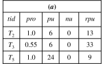
Figure 1: Constructed PU^±-list of pattern $\{a\})$

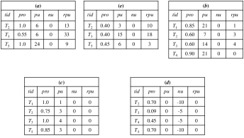
Figure 2: Constructed PU^±-list of the running example

Example 5

The search space of the developed HUPNU approach can be shown as the utility-based Set-enumeration tree [37], called a PU^±-tree, based on the developed PU^±-list. Since {$RTWU(a)$: $185; $RTWU(b)$: $259; $RTWU(c)$: $202; $RTWU(d)$: $231; and $RTWU(e)$: $285}, the designed processing order $\succ$ of the running example can be represented as: $\{a\succ d\succ b\succ e\succ c\}$. Thus, the constructed PU^±-list for all items in Table I is shown in Fig. 2. We have $\{a\}.PUL$ = $\{(T_{1}$, 0.60, $40, $0, $67), $(T_{3}$, 1.00, $32, -$4, $22), $(T_{5}$, 0.90, $24, -$2, $0)}; $\{c\}.PUL$ = $\{(T_{2}$, 0.75, $0, -$2, $0), $(T_{3}$, 0.70, $0, -$4, $0), $(T_{4}$, 0.90, $0, -$2, $0), $(T_{5}$, 0.95, $0, -$8, $0)}; $\{a,c\}.PUL$ = $\{T_{3}$, 0.70, $32, -$4, $0), $(T_{4}$, 0.81, $24, -$2, $0)}.

Definition 6

The sums of the total utility, pu values, nu values, and rpu values in the PU^±-list of X are respectively denoted as: SUM(X.iu), SUM(X.pu), SUM(X.nu), and SUM(X.rpu), which can be respectively defined as:
$SUM(X.pu)$ = $\sum_{X\in T_{c}\wedge T_{c}\subseteq D}X.pu(T_{c})$;
$SUM(X.nu)$ = $\sum_{X\in T_{c}\wedge T_{c}\subseteq D}X.nu(T_{c})$;
$SUM(X.rpu)$ = $\sum_{X\in T_{c}\wedge T_{c}\subseteq D}X.rpu(T_{c})$;
$SUM(X.iu)$ = $SUM(X.pu)$ + $SUM(X.nu)$.

Lemma 1

For two patterns, such as Y and Z in the PU^±-tree, if the relationship holds: (1) $SUM(Y.pu)+SUM(Y.rpu)$ - $\sum_{\forall T_{c}\in D,Y\subseteq T_{c}\bigwedge Z\nsubseteq T_{c}}(Y.pu+Y.rpu)<minUtil$, or (2) $SUM(Y.pro)$ - $\sum_{\forall T_{c}\in D,Y\subseteq T_{c}\bigwedge Z\nsubseteq T_{c}}(Y.pro)<minPro\times|D|$, the (YZ), or any superset of it, will not be a PHUI.

Strategy 1 (PU-Prune strategy)

If Lemma 1 holds, then the PU^±-list construction of the pattern $Y$ can be avoided; and any of its superset will not be a PHUI.

According to the designed PU-Prune strategy, the huge size of the unpromising k-patterns (k $\geq$ 2, and $k$ is the size of the items within the itemset) of the search space can be greatly filtered. Let $Py$ denote an itemset, and $y$ denote an item; $Py$ is defined as $P\cup y$ and y is before z. The construction procedure of the PU^±-list is shown in Algorithm 1. It takes the PU^±-lists of $P$, $Py$, and $Pz$ as the inputs, and returns the PU^±-list of $Pyz$ as output. The PU^±-lists of $k$-itemsets ($k\geq$ 2) can be easily built using a simple join operation of (k-1)-itemsets; multiple database scans can be greatly avoided, and the computational cost of the run time can be reduced. If $P.PUL$ is empty, the PU^±-list of a 2-itemset is constructed (Line 9). Otherwise, the PU^±-list of a $k$-itemset ($k\geq$ 3) is constructed (Lines 5 to 7). For these optimization purposes, the joint operation of the PU^±-lists of $P$, $Py$, and $Pz$ can be constructed by a binary search.

Algorithm 1 Construction procedure

0:  $P$, $Py$, $Pz$.

0:  Pyz with its Pyz.PUL.

1:  $Pyz.PUL\leftarrow\emptyset$;

2:  set $Probability$ = SUM$(Y.pro)$, $Utility$ = SUM$(Y.pu)$ + SUM$(Y.rpu)$;

3:  for each tuple $ex\in Py.PUL$ do

4:     if $\exists ez\in Pz.PUL$ and $ey.tid$ = $eyz.tid$ then

5:        if $P.PUL\neq\emptyset$  then

6:           search each element $e\in P.PUL$ such that $e.tid$ = $ey.tid$.;

7:           $eyz\leftarrow$ $<$$ey.tid,ey.pro\times ez.pro/e.pro$, $ey.pu+ez.pu-e.pu$, $ey.nu+ez.nu-e.nu$, $ez.rpu$$>$;

8:        else

9:           $eyz\leftarrow$ $<$$ey.tid,ey.pro\times ez.pro$, $ey.pu+ez.pu$, $ey.nu+ez.nu,ez.rpu$$>$;

10:        end if

11:        $Pyz.PUL\leftarrow Pyz.PUL\cup\{eyz\}$;

12:     else

13:        Probability = Probability - ey.pro, Utility = Utility - ey.pu - ey.rpu;

14:        if Probability $<minPro\times|D|$ or $Utility<minUtil$  then

15:           return null.

16:        end if

17:     end if

18:  end for

19:  return Pyz

IV-C Proposed Pruning Strategies

In this section, we discuss several pruning strategies based on the developed PU^±-list for later mining progress. The developed strategies can greatly help to remove the uncompromising candidates in the early stages, and thus the search space that reveals the actual PHUIs can become smaller. The node of the (k-1)-itemset in the designed PU^±-tree is denoted as: $X^{k-1}(k\geq 2)$, and any superset of it is denoted as: $X^{k}$.

Theorem 1 (Downward closure property of RTWU and probability)

In the PU^±-tree, the correctness of $Pro(X^{k-1})\geq Pro(X^{k})$ and RTWU(X^k-1) $\geq$ RTWU(X^k) hold.

Proof:

Since $p(X,T_{c})$ = $\prod_{i\in X}p(i,T_{c})$ can be held for any $T_{c}$ in $D$, thus we can have that: $p(X^{k},T_{c})\leq p(X^{k-1},T_{c})$. Since $X^{k-1}$ is the subset of $X^{k}$; the $tids$ of $X^{k}$ is the subset of the $tids$ of $X^{k-1}$. We then can have that: $Pro(X^{k})$ = $\sum_{X^{k}\subseteq T_{c}\wedge T_{c}\in D}p(X^{k},T_{c})$ $\leq\sum_{X^{k-1}\subseteq T_{c}\wedge T_{c}\in D}p(X^{k-1},T_{c})$ = $Pro(X^{k-1})$. Thus, it can be concluded that Pro(X^k-1) $\geq$ Pro(X^k). Moreover, X${}^{\textit{k}-1}$ $\subseteq$ X^k, $RTWU(X^{k})$ = $\sum_{X^{k}\subseteq T_{c}\wedge T_{c}\in D}tu(T_{c})$ $\leq\sum_{X^{k-1}\subseteq T_{c}\wedge T_{c}\in D}tu(T_{c})$ = $RTWU(X^{k-1})$ holds. ∎

Lemma 2 (Upper-bound probability of PHUI)

The summed up probability of any node in the PU^±-tree is greater than the summed up probabilities of its supersets.

Strategy 2

The RTWU and the probability value of each item can be easily obtained during the initial database scan. Thus, if the summed up probability and RTWU of an itemset X do not achieve the two conditions of PHUI, X and any supersets of it can be pruned directly.

Strategy 3

While the depth-first search is performed to traverse the PU^±-tree, if the summed up probability of tree node X such as $Pro(X)$ is no larger than $minPro\times|D|$, then none of the supersets of this node are considered to be a PHUI.

Lemma 3 (Upper-bound utility of the PHUI)

For a node X in the PU^±-tree, the summed values of $SUM(X.pu)$ and $SUM(X.rpu)$ are always equal to or larger than any of its supersets.

We can conclude from the above lemmas that the summed up utility w.r.t. $u(X^{k})$ of an itemset $X^{k}$ is always no greater than the summed values of SUM$(X^{k-1}.pu)$ and SUM$(X^{k-1}.rpu)$. Therefore, it is ensured that the transitive extensions with items having positive or negative utilities can hold the downward closure property. The following strategies can be designed based on the above upper-bound constraints:

Strategy 4

While the depth-first search is performed to traverse the PU^±-tree, if the summed up values of SUM$(X^{k-1}.pu)$ and SUM$(X^{k-1}.rpu)$ are less than $minUtil$, any supersets of X cannot be a PHUI. Those nodes in the tree can be directly ignored and pruned to reduce the search space for mining the PHUIs.

Strategy 5

For an itemset X in the PU^±-list, if the X.PUL is null or the $Pro(X)$ value is less than $minPro\times|D|$, X cannot be considered a PHUI; none of its superset (node) is a PHUI. Therefore, the construction procedure of PU^±-lists of X’s supersets can be ignored.

The efficient Estimated Utility Co-occurrence Pruning (EUCP) strategy [42] is also utilized here for the designed HUPNU algorithm. Thus, the Estimated Utility Co-occurrence Structure (EUCS) is built to keep the RTWU values of the 2-itemsets. More information can be found in [42].

Strategy 6

Let $X$ be a 2-itemset, which is also one of the nodes in the Set-enumeration PU^±-tree. While the depth-first search is performed, if the RTWU of $X$ is no greater than the $minUtil$ based on the built EUCS, X and any supersets of X are not considered to be the PHUI; the construction progress of the PU^±-tree for X and the supersets of it can be ignored.

Based on the above proposed pruning strategies, the designed HUPNU is shown in detail below.

IV-D The Procedure of HUPNU

In this section, the main procedure of the developed HUPNU is shown in Algorithm 2. First, it examines the uncertain database to find the values of RTWU (with the redefined $RTU$) and $Pro(i)$ of each item (Line 1). The expected support and RTWU of each item in the set $I^{*}$ are then checked against the $minPro\times|D|$ and $minUtil$, respectively, and the satisfied items are then discovered and obtained. In this step, the other items can be ignored directly since they could not be the potential HUI (Line 2). The database is then scanned again (Line 4) to re-order the items in the transactions according to the designed order as $\succ$ (Line 3). In addition, the items in the transactions are then re-ordered based on the total order $\succ$ while performing the database scan. After that, the PU^±-list of each 1-item $i\in I^{*}$ is constructed, respectively, and the depth-first search is recursively performed by the Search procedure with the empty itemset $\emptyset$, the set of single items $I^{*}$, minPro, minUtil, and the EUCS (Line 5).

Algorithm 2 HUPNU main procedure

0:  $D$, minPro, minUtil, ptable.

0:  The set of PHUIs.

1:  scan uncertain database $D$ to calculate the RTWU$(i)$ and $Pro(i)$ of each item $i\in I$;

2:  $I^{*}\leftarrow$ each item $i$ such that $Pro(i)\geq minPro\times|D|\wedge RTWU(i)\geq minUtil$;

3:  sort the items in the set of $I^{*}$ as $\succ$ order;

4:  scan database $D$ to build the PU^±-list of each item $i\in I^{*}$ and construct $EUCS$;

5:  call Search($\emptyset$, $I^{*}$, minPro, minUtil, EUCS).

6:  return PHUIs

Algorithm 3 Search procedure

0:  $P$, ExtensionsOfP, minPro, minUtil, EUCS.

0:  The set of PHUIs.

1:  for each pattern $Py\in$ ExtensionsOfP do

2:     if SUM(Py.pro) $\geq minPro\times|D|$ $\wedge$ (SUM(Py.pu) + SUM(Py.nu)) $\geq minUtil$ then

3:        output $Py$ as a PHUI;

4:     end if

5:     if SUM(Py.pro) $\geq minPro\times|D|$ $\wedge$ (SUM(Py.pu) + SUM(Py.rpu)) $\geq minUtil$ then

6:        ExtensionsOfPy $\leftarrow\emptyset$;

7:        for $Pz\in$ ExtensionsOfP such that $z\succ y$ do

8:           if $RTWU(\{y,z\})\geq minUtil$ then

9:              $Pyz\leftarrow Py\cup Pz$;

10:              Pyz.PUL $\leftarrow$ Construct(P, Py, Pz);

11:              if Pyz.PUL $\not=\emptyset$ and SUM(Pyz.pro) $\geq minPro$ $\times|D|$ then

12:                 ExtensionsOfPy $\leftarrow$ ExtensionsOfPy $\cup Pyz$;

13:              end if

14:           end if

15:        end for

16:        call Search(Pyz, ExtensionsOfPy, minPro, minUtil, EUCS).

17:     end if

18:  end for

19:  return PHUIs

The search procedure of the HUPNU is described in Algorithm 3. For each extension $Py$ of $P$, if the probability of $Py$ is no less than $minPro\times|D|$, and the summed up actual utility of $Py$ in the PU^±-list (denoted as SUM$(Y.pu)$ + SUM$(Y.nu)$) is no less than $minUtil$, then $Py$ can be considered to be a PHUI (Lines 2 to 4). The developed pruning Strategies 3 and 4 are then performed to check whether the extension ($Py$) can be explored (Line 5). This progress can be executed by integrating $Py$ with all extensions $Pz$ of $P$, such that $z\succ y$ and $RTWU(\{y,z\})\geq minUtil$ (Line 8, pruning Strategy 6), to generate the extensions ($Pyz$) containing $|Py|+1$ items. After that, the PU^±-list of $Pyz$ can be built by the Construct procedure to join the PU^±-lists of $P$, $Py$, and $Pz$ (Lines 9 to 13). Note that the promising PU^±-lists can only be later explored (Line 12, pruning Strategy 5). A recursive $Search$ procedure of $Pyz$ is then performed to obtain its utility and explore the extension(s) (Line 16).

V Experimental Study

In this section, we evaluate the performance of the developed HUPNU algorithm. All the algorithms were implemented with Java language, and executed on an Intel Core-i5 processor running on Microsoft Windows 7 64 bits operation system with 4GB of main memory. Memory usage was measured by Java API. To the best of our knowledge, this is the first paper that considers both the positive and negative unit utilities of items in an uncertain database; none of the previous works handle this topic. Thus, the developed HUPNU along with several designed pruning strategies were compared in the experiments. HUPNU_P12 denotes that pruning Strategies 1 and 2 were involved in the HUPNU; HUPNU_P123 considers pruning Strategies 1, 2, and 3; HUPNU_P1234 takes the pruning Strategies 1, 2, 3, and 4; and HUPNU_All is concerned with all the pruning Strategies (1 to 5) for evaluation. Experiments were carried out on five realistic datasets (i.e., kosarak, accidents, psumb, retail, and mushroom) and one synthetic dataset [43]. The individual characteristics of each of the six datasets are given below.

• kosarak: it has 990,002 transactions, and the number of distinct items is 41,270. The average length and the maximum length of transactions are is 8.09 and 2,498, respectively.

• accidents: it has 340,183 transactions and 468 distinct items. For the all transactions, the average length is 33.8 and the maximum length is 51.

• psumb: it has total 49,046 transactions and 2,113 distinct items. It is a very dense dataset since the average length of each transaction is 74.

• retail: this dataset contains 88,162 transactions and total 16,470 distinct items. The average length of transactions is 10.3, and the maximum length is 76.

• mushroom: it has 8,124 transactions with 119 distinct items. It is a dense dataset since both the average length and the maximum length are 23.

• T10I4D100K [43]: this dataset has 100,000 transactions with 870 items. These transactions have average 10.1 items, and the maximum length is 29.

The external utilities of different items for the six datasets were generated in the range of [-1,000, 1,000] using a log-normal distribution. In addition, the quantities of the items were randomly generated in the range of [1, 5]. These settings are similar to the previous well-known algorithms [7, 42, 8] for HUPM. Moreover, the unique probabilities of the items were randomly assigned in the range of (0.0, 1.0). In the experiments, we evaluated the implemented algorithms in terms of runtime, number of visited nodes (or patterns), and scalability. The results are given below.

V-A Evaluation of Runtime

The runtime of the four implemented algorithms were then compared under the variants of minUtil and minPro thresholds. Results in terms of the two thresholds are shown in Fig. 3 and Fig. 4, respectively.

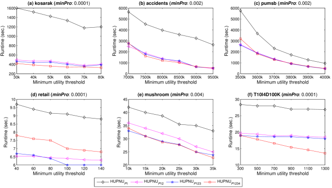
Figure 3: Runtime under varied minUtil with a fixed minPro.

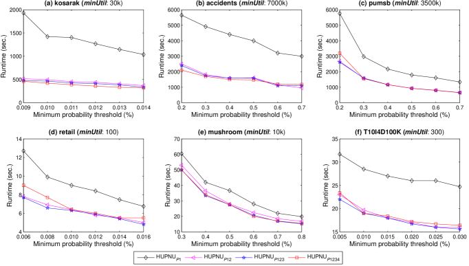
Figure 4: Runtime under varied minPro with a fixed minUtil.

As shown in Fig. 3 and Fig. 4, the runtimes of all implemented algorithms decreased along with the increasing of the $minUtil$ or $minPro$ threshold. Specifically, the implemented algorithms with variants of pruning strategies greatly improved the performance, up to nearly one or two orders of magnitude faster than the baseline approach. For example, HUPNU_P1234, which adopts all the efficient pruning strategies, outperformed the other variants of the designed approach. The reason is that the HUPNU_P1234 algorithm is concerned with all the pruning strategies, and the unpromising candidates can be greatly reduced. Therefore, the traversal procedure to explore the unpromising patterns in the enumeration tree can be avoided, as well as the costly join operation to generate the huge unpromising candidates of the PU^±-lists. When the minUtil and minPro values were set lower, more and longer patterns were mined, and there was a greater computational cost in terms of the runtime that was required. This situation can be easily observed in a very dense dataset, for example in accidents and psumb.

The developed PU^±-list can also easily help the variants of the algorithms to directly mine the required patterns without candidate generation. The list structure can effectively reduce the multiple database scans. We can also observe that the designed pruning strategies can greatly help with reducing the number of unpromising patterns. The required memory usage of the variants of algorithms is much less, but due to the page limit, we omit some details of the results. However, in the general pattern-mining approach, it can be easily concluded that more memory usage was required when the threshold was set lower. The designed PU^±-list could actually solve this limitation by using a more compressed search space, and achieve effectiveness and efficiency for mining the PHUIs.

V-B Evaluation of Number of Patterns (Visited Nodes)

In this section, the numbers of visited nodes (also known as the candidate patterns) in the designed PU^±-tree are compared to evaluate the effects of pruning strategies. Note that the number of visited nodes of the four variants of the HUPNU algorithm is denoted as $N_{1}$, $N_{2}$, $N_{3}$, and $N_{4}$, respectively. According to the same parameter settings in Fig. 3 and Fig. 4, the final results of the patterns are respectively shown in Table II and Table III in terms of minUtil and minPro thresholds.

From Table II and Table III, it can be seen that $N_{1}>N_{2}>N_{3}>N_{4}>$ PHUIs in terms of varied minUtil and minPro. We can then draw a conclusion such that: (1) The number of designed PHUIs discovered was fewer in the uncertain dataset compared to the number of candidate patterns. (2) The set of the discovered PHUIs was more meaningful; the designed HUPNU discover more concrete and useful patterns with both positive and negative unit utilities of item constraints than the traditional algorithms in HUPM. (3) The search space of the HUPNU was very large without any pruning strategies, but the developed strategies could reduce the its size. (4) The results were reasonable, and even the size of the search space could be reduced by different pruning strategies, the completeness, and the correctness of the final PHUIs could still be held.

For the designed pruning strategies 2, 3, and 4 of the implemented HUPNU_P1 algorithm, they hold the upper-bound values for the utility and probability of the patterns, and thus combinational exploration could be avoided. However, some unpromising patterns could not be effectively filtered, which can be obviously seen from the gap between the number of final PHUIs and $N_{1}$. It can also be seen that PU-Prune had a great performance in removing unpromising patterns, which could be observed in $N_{1}$ and $N_{2}$. This strategy avoids the construction progress for the numerous unpromising patterns. We can also see that the EUCP strategy made a great effort to reduce the search space. The relationships of $N_{1}>N_{2}>N_{3}>N_{4}$ were correctly held. When the threshold value was set lower, for example, $minUtil$ or $minPro$, the gap between different implemented algorithms of the visited patterns could become huge, and the effectiveness of the designed pruning strategies is held.

TABLE II: Derived patterns under varied minUtil and fixed minPro

Dataset	Pattern	Threshold of minUtil
		$minUtil_{1}$	$minUtil_{2}$	$minUtil_{3}$	$minUtil_{4}$	$minUtil_{5}$	$minUtil_{6}$
	$N_{1}$	109,475,579	79,746,008	61,798,333	50,499,186	41,197,757	33,144,921
	$N_{2}$	14,399,980	12,180,884	10,571,745	9,254,740	8,123,221	7,125,357
(a) kosarak	$N_{3}$	12,322,701	10,611,814	9,369,910	8,286,105	7,345,445	6,505,338
	$N_{4}$	8,067,669	6,811,140	5,945,495	5,217,922	4,603,638	4,081,767
	PHUIs	45,613	35,662	28,077	24,317	21,420	18,843
	$N_{1}$	194,512	163,169	138,399	120,560	107,620	96,807
	$N_{2}$	147,052	119,802	98,237	83,198	72,963	64,390
(b) accidents	$N_{3}$	146,426	119,140	97,507	82,366	72,087	63,486
	$N_{4}$	144,957	117,671	96,038	80,897	70,618	62,017
	PHUIs	6,331	5,462	4,603	3,940	3,493	3,120
	$N_{1}$	2,522,059	1,814,071	1,365,950	1,184,769	1,059,297	849,484
	$N_{2}$	1,265,985	801,074	590,923	490,411	434,835	342,120
(c) pumsb	$N_{3}$	1,238,118	795,362	583,778	484,847	423,414	337,667
	$N_{4}$	1,236,179	793,423	581,839	482,908	421,475	335,732
	PHUIs	8,648	4,123	3,114	1,773	1,388	1,238
	$N_{1}$	96,139,509	48,350,235	35,111,699	27,307,914	21,761,430	17,948,378
	$N_{2}$	21,876,139	17,735,518	15,582,757	13,731,190	11,813,940	10,462,617
(d) retail	$N_{3}$	21,078,117	17,429,475	15,360,149	13,568,770	11,696,475	10,374,338
	$N_{4}$	20,968,980	17,332,324	15,270,502	13,484,318	11,615,439	10,296,705
	PHUIs	19,278	13,584	10,655	8,747	7,423	6,378
	$N_{1}$	1,558,452	974,145	721,233	507,260	380,254	322,867
	$N_{2}$	828,898	527,865	394,426	278,595	215,407	181,517
(e) mushroom	$N_{3}$	700,121	440,243	327,442	229,328	175,038	146,840
	$N_{4}$	698,969	439,522	326,867	228,871	174,672	146,516
	PHUIs	147,088	85,133	62,773	42,466	30,510	25,590
	$N_{1}$	14,059,513	7,194,329	4,743,728	3,475,577	2,739,103	2,257,562
	$N_{2}$	6,199,289	2,365,166	1,264,020	820,482	607,506	491,439
(f) T10I4D100K	$N_{3}$	4,619,226	1,655,006	872,646	584,661	453,250	383,900
	$N_{4}$	4,454,919	1,570,317	802,457	519,180	390,542	323,262
	PHUIs	37,242	20,710	13,916	10,140	7,854	6,292

TABLE III: Derived patterns under varied minPro and fixed minUtil

Dataset	Pattern	Threshold of minPro
		$minPro_{1}$	$minPro_{2}$	$minPro_{3}$	$minPro_{4}$	$minPro_{5}$	$minPro_{6}$
	$N_{1}$	79,746,008	73,064,534	66,950,091	61,745,111	57,114,432	53,014,125
	$N_{2}$	12,180,884	11,778,729	11,445,291	11,154,865	10,808,309	10,460,194
(a) kosarak	$N_{3}$	10,611,814	10,375,295	10,205,956	10,077,832	9,882,828	9,664,443
	$N_{4}$	6,811,140	6,028,964	5,459,093	5,019,367	4,612,615	4,243,295
	PHUIs	35,662	24,589	17,304	12,595	9,362	7,154
	$N_{1}$	194,512	150,179	112,717	84,525	64,389	48,824
	$N_{2}$	147,052	109,522	81,229	60,283	44,655	32,550
(b) accidents	$N_{3}$	146,426	109,127	80,933	60,098	44,554	32,490
	$N_{4}$	144,957	107,740	79,657	59,029	43,610	31,651
	PHUIs	6,331	4,552	3,321	2,411	1,735	1,237
	$N_{1}$	2,522,059	1,892,203	1,433,997	1,054,904	780,328	600,511
	$N_{2}$	1,265,985	904,469	654,212	473,337	344,866	256,833
(c) pumsb	$N_{3}$	1,238,118	885,941	642,025	466,156	340,510	254,184
	$N_{4}$	1,236,179	883,884	640,104	464,472	338,917	252,599
	PHUIs	8,648	5,582	3,630	2,277	1,396	817
	$N_{1}$	37,793,976	37,017,817	36,106,601	35,111,699	34,139,328	33,094,290
	$N_{2}$	16,931,811	16,454,728	15,986,124	15,582,757	15,288,602	15,031,344
(d) retail	$N_{3}$	16,526,029	16,131,265	15,715,903	15,360,149	15,101,236	14,876,214
	$N_{4}$	16,507,082	16,090,920	15,652,668	15,270,502	14,984,007	14,728,697
	PHUIs	14,406	13,048	1,1802	10,655	9,660	8,724
	$N_{1}$	974,145	923,770	860,295	796,159	727,630	665,124
	$N_{2}$	527,865	485,700	444,208	404,089	363,959	328,273
(e) mushroom	$N_{3}$	440,243	406,109	373,114	341,243	309,047	281,344
	$N_{4}$	439,522	405,048	372,035	339,920	307,708	279,939
	PHUIs	85,133	75,769	67,538	60,065	52,944	47,398
	$N_{1}$	7,194,329	6,992,960	6,804,076	6,632,844	6,457,696	6,259,347
	$N_{2}$	2,365,166	2,195,551	2,034,389	1,879,105	1,718,748	1,549,820
(f) T10I4D100K	$N_{3}$	1,655,006	1,519,652	1,398,078	1,296,955	1,211,962	1,133,041
	$N_{4}$	1,570,317	1,384,445	1,225,810	1,097,950	997,283	905,622
	PHUIs	20,710	19,278	17,869	16,454	15,132	13,900

V-C Evaluation of Scalability

From Fig. 5, the scalability was carried out on a realistic BMS-POS dataset under varied dataset sizes. The threshold values were set as minPro = 0.0001 and minUtil = 10k, and the dataset size was varied from 100k to 500k. In Fig. 5(a), we can then find that the runtimes of the four implemented algorithms linearly increased along with the increasing size of the dataset. We can see that the runtime of HUPNU_P123 was close to that of HUPNU_P12, and both of them were significantly faster than HUPNU_P1. We also can see that HUPNU_P1234 outperformed the other implemented algorithms. When the size of the dataset increases, the gap between the implemented algorithms becomes larger but they still remain stable with linear growth. The memory usage of four implemented algorithms is shown in Fig. 5(b). HUPNU_P1 requires the most memory usage; HUPNU_P123 and HUPNU_P1234 has similar results, and requires the least memory usage. Fig. 5(c) shows the number of visited patterns of the four implemented algorithms and the final PHUIs. The results show the effectiveness and efficiency of the designed pruning strategies, and when the size of the dataset becomes larger, the gap of those algorithms becomes huge.

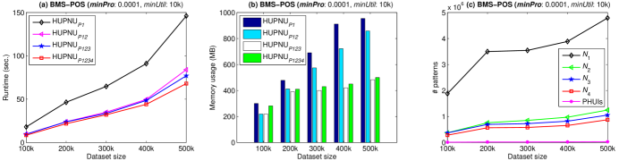
Figure 5: Scalability evaluation.

VI Conclusion

In this paper, we present a HUPNU algorithm by jointly considering the uncertainty and utility (both positive and negative) factors, to reveal the qualified high-utility patterns. This is the first work concerning these realistic factors in some real-life situations, such as Internet of Things data and manufacturing data. A vertical structure named PU^±-list was designed to keep necessary information, such as probability, and the positive and negative utilities of the items for later mining progress. Based on the above properties, the HUPNU algorithm could directly produce the qualified high-utility patterns in one phase. Moreover, several efficient pruning strategies were also developed to greatly reduce the search space for mining the promising patterns, and thus the computation could be sped up efficiently. Extensive experiments were carried out on several synthetic/realistic datasets to show the efficiency and effectiveness of the designed algorithm in terms of runtime, number of discovered qualified patterns, and scalability.

References

- [1] L. Atzori, A. Iera, and G. Morabito, “The internet of things: A survey,” Computer Networks, vol. 54, no. 15, pp. 2787–2805, 2010.
- [2] C. W. Tsai, C. F. Lai, M. C. Chiang, L. T. Yang et al., “Data mining for internet of things: A survey.” IEEE Communications Surveys and Tutorials, vol. 16, no. 1, pp. 77–97, 2014.
- [3] F. Chen, P. Deng, J. Wan, D. Zhang, A. V. Vasilakos, and X. Rong, “Data mining for the internet of things: literature review and challenges,” International Journal of Distributed Sensor Networks, vol. 11, no. 8, p. 431047, 2015.
- [4] R. Agrawal, R. Srikant et al., “Fast algorithms for mining association rules,” in Proceedings of the 20th International Conference on very Large Databases, vol. 1215, 1994, pp. 487–499.
- [5] J. Han, J. Pei, Y. Yin, and R. Mao, “Mining frequent patterns without candidate generation: A frequent-pattern tree approach,” Data Mining and Knowledge Discovery, vol. 8, no. 1, pp. 53–87, 2004.
- [6] C. F. Ahmed, S. K. Tanbeer, B. S. Jeong, and Y. K. Lee, “Efficient tree structures for high utility pattern mining in incremental databases,” IEEE Transactions on Knowledge and Data Engineering, vol. 21, no. 12, pp. 1708–1721, 2009.
- [7] M. Liu and J. Qu, “Mining high utility itemsets without candidate generation,” in Proceedings of the 21st ACM International Conference on Information and Knowledge Management. ACM, 2012, pp. 55–64.
- [8] V. S. Tseng, B. E. Shie, C. W. Wu, and P. S. Yu, “Efficient algorithms for mining high utility itemsets from transactional databases,” IEEE Transactions on Knowledge and Data Engineering, vol. 25, no. 8, pp. 1772–1786, 2013.
- [9] Z. Sheng, S. Yang, Y. Yu, A. Vasilakos, J. Mccann, and K. Leung, “A survey on the ietf protocol suite for the internet of things: Standards, challenges, and opportunities,” IEEE Wireless Communications, vol. 20, no. 6, pp. 91–98, 2013.
- [10] P. Fournier-Viger, J. C. W. Lin, B. Vo, T. T. Chi, J. Zhang, and H. B. Le, “A survey of itemset mining,” Wiley Interdisciplinary Reviews: Data Mining and Knowledge Discovery, vol. 7, no. 4, 2017.
- [11] U. Yun, G. Lee, and E. Yoon, “Efficient high utility pattern mining for establishing manufacturing plans with sliding window control,” IEEE Transactions on Industrial Electronics, vol. 64, no. 9, pp. 7239–7249, 2017.
- [12] F. Tao, Y. Cheng, L. Zhang, and D. Zhao, “Utility modelling, equilibrium, and coordination of resource service transaction in service-oriented manufacturing system,” Proceedings of the Institution of Mechanical Engineers, Part B: Journal of Engineering Manufacture, vol. 226, no. 6, pp. 1099–1117, 2012.
- [13] W. Gan, J. C. W. Lin, P. Fournier-Viger, H. C. Chao, V. S. Tseng, and P. S. Yu, “A survey of utility-oriented pattern mining,” arXiv preprint arXiv:1805.10511, 2018.
- [14] Y. W. Teng, C. H. Tai, P. S. Yu, and M. S. Chen, “Revenue maximization on the multi-grade product,” in Proceedings of the SIAM International Conference on Data Mining. SIAM, 2018, pp. 576–584.
- [15] C. H. Cai, A. W. C. Fu, C. Cheng, and W. Kwong, “Mining association rules with weighted items,” in International Database Engineering and Applications Symposium. IEEE, 1998, pp. 68–77.
- [16] C. J. Chu, V. S. Tseng, and T. Liang, “An efficient algorithm for mining high utility itemsets with negative item values in large databases,” Applied Mathematics and Computation, vol. 215, no. 2, pp. 767–778, 2009.
- [17] J. Wan, S. Tang, D. Li, S. Wang, C. Liu, H. Abbas, and A. V. Vasilakos, “A manufacturing big data solution for active preventive maintenance,” IEEE Transactions on Industrial Informatics, vol. 13, no. 4, pp. 2039–2047, 2017.
- [18] C. C. Aggarwal and P. S. Yu, “A survey of uncertain data algorithms and applications,” IEEE Transactions on Knowledge and Data Engineering, vol. 21, no. 5, pp. 609–623, 2009.
- [19] T. Bernecker, H. P. Kriegel, M. Renz, F. Verhein, and A. Zuefle, “Probabilistic frequent itemset mining in uncertain databases,” in Proceedings of the 15th ACM SIGKDD International Conference on Knowledge Discovery and Data Mining. ACM, 2009, pp. 119–128.
- [20] J. C. W. Lin, W. Gan, P. Fournier-Viger, T. P. Hong, and V. S. Tseng, “Efficient algorithms for mining high-utility itemsets in uncertain databases,” Knowledge-Based Systems, vol. 96, pp. 171–187, 2016.
- [21] Y. Liu, X. Weng, J. Wan, X. Yue, H. Song, and A. V. Vasilakos, “Exploring data validity in transportation systems for smart cities,” IEEE Communications Magazine, vol. 55, no. 5, pp. 26–33, 2017.
- [22] L. Geng and H. J. Hamilton, “Interestingness measures for data mining: A survey,” ACM Computing Surveys, vol. 38, no. 3, p. 9, 2006.
- [23] J. M. Luna, A. Cano, M. Pechenizkiy, and S. Ventura, “Speeding-up association rule mining with inverted index compression,” IEEE Transactions on Cybernetics, vol. 46, no. 12, pp. 3059–3072, 2016.
- [24] R. Srikant and R. Agrawal, “Mining sequential patterns: Generalizations and performance improvements,” in International Conference on Extending Database Technology. Springer, 1996, pp. 1–17.
- [25] T. P. Hong, C. S. Kuo, and S. C. Chi, “Mining association rules from quantitative data,” Intelligent Data Analysis, vol. 3, no. 5, pp. 363–376, 1999.
- [26] C. K. Chui, B. Kao, and E. Hung, “Mining frequent itemsets from uncertain data,” in Pacific-Asia Conference on Knowledge Discovery and Data Mining. Springer, 2007, pp. 47–58.
- [27] H. Yao, H. J. Hamilton, and C. J. Butz, “A foundational approach to mining itemset utilities from databases,” in Proceedings of the SIAM International Conference on Data Mining. SIAM, 2004, pp. 482–486.
- [28] Y. Liu, W. k. Liao, and A. Choudhary, “A two-phase algorithm for fast discovery of high utility itemsets,” in Pacific-Asia Conference on Knowledge Discovery and Data Mining. Springer, 2005, pp. 689–695.
- [29] C. W. Tsai, C. F. Lai, H. C. Chao, and A. V. Vasilakos, “Big data analytics: a survey,” Journal of Big Data, vol. 2, no. 1, p. 21, 2015.
- [30] J. C. W. Lin, W. Gan, T. P. Hong, and V. S. Tseng, “Efficient algorithms for mining up-to-date high-utility patterns,” Advanced Engineering Informatics, vol. 29, no. 3, pp. 648–661, 2015.
- [31] J. C. W. Lin, J. Zhang, P. Fournier-Viger, T. P. Hong, and J. Zhang, “A two-phase approach to mine short-period high-utility itemsets in transactional databases,” Advanced Engineering Informatics, vol. 33, pp. 29–43, 2017.
- [32] J. C. W. Lin, W. Gan, and T. P. Hong, “A fast updated algorithm to maintain the discovered high-utility itemsets for transaction modification,” Advanced Engineering Informatics, vol. 29, no. 3, pp. 562–574, 2015.
- [33] W. Gan, J. C. W. Lin, P. Fournier-Viger, H. C. Chao, T. P. Hong, and H. Fujita, “A survey of incremental high-utility itemset mining,” Wiley Interdisciplinary Reviews: Data Mining and Knowledge Discovery, vol. 8, no. 2, 2018.
- [34] J. C. W. Lin, W. Gan, and T. P. Hong, “A fast maintenance algorithm of the discovered high-utility itemsets with transaction deletion,” Intelligent Data Analysis, vol. 20, no. 4, pp. 891–913, 2016.
- [35] J. C. W. Lin, W. Gan, P. Fournier-Viger, T. P. Hong, and V. S. Tseng, “Fast algorithms for mining high-utility itemsets with various discount strategies,” Advanced Engineering Informatics, vol. 30, no. 2, pp. 109–126, 2016.
- [36] V. S. Tseng, C. W. Wu, P. Fournier-Viger, and P. S. Yu, “Efficient algorithms for mining the concise and lossless representation of high utility itemsets,” IEEE Transactions on Knowledge and Data Engineering, vol. 27, no. 3, pp. 726–739, 2015.
- [37] J. C. W. Lin, W. Gan, P. Fournier-Viger, T. P. Hong, and H. C. Chao, “FDHUP: Fast algorithm for mining discriminative high utility patterns,” Knowledge and Information Systems, vol. 51, no. 3, pp. 873–909, 2017.
- [38] V. S. Tseng, C. W. Wu, P. Fournier-Viger, and P. S. Yu, “Efficient algorithms for mining top- high utility itemsets,” IEEE Transactions on Knowledge and Data Engineering, vol. 28, no. 1, pp. 54–67, 2016.
- [39] W. Gan, J. C. W. Lin, P. Fournier-Viger, H. C. Chao, and P. S. Yu, “HUOPM: High utility occupancy pattern mining,” arXiv preprint arXiv:1812.10926, 2018.
- [40] G. C. Lan, T. P. Hong, J. P. Huang, and V. S. Tseng, “On-shelf utility mining with negative item values,” Expert Systems with Applications, vol. 41, no. 7, pp. 3450–3459, 2014.
- [41] J. C. W. Lin, P. Fournier-Viger, and W. Gan, “FHN: An efficient algorithm for mining high-utility itemsets with negative unit profits,” Knowledge-Based Systems, vol. 111, pp. 283–298, 2016.
- [42] P. Fournier-Viger, C. W. Wu, S. Zida, and V. S. Tseng, “FHM: Faster high-utility itemset mining using estimated utility co-occurrence pruning,” in International Symposium on Methodologies for Intelligent Systems. Springer, 2014, pp. 83–92.
- [43] R. Agrawal and R. Srikant, “Quest synthetic data generator. http://www.Almaden.ibm.com/cs/quest/syndata.html,” 1994.