Theory for the optimal detection of time-varying signals in cellular sensing systems

Abstract

Living cells often need to measure chemical concentrations that vary in time. To this end, they deploy many resources such as receptors, downstream signaling molecules, time and energy. Here, we present a theory for the optimal design of a large class of sensing systems that need to detect time-varying signals, a receptor driving a push-pull network. The theory is based on the concept of the dynamic input-output relation, which describes the mapping between the current ligand concentration and the average receptor occupancy over the past integration time. This concept is used to develop the idea that the cell employs its push-pull network to estimate the receptor occupancy and then uses this estimate to infer the current ligand concentration by inverting the dynamic input-output relation. The theory reveals that the sensing error can be decomposed into two terms: the sampling error in the estimate of the receptor occupancy and the dynamical error that arises because the average ligand concentration over the past integration time may not reflect the current ligand concentration. The theory generalizes the design principle of optimal resource allocation previously identified for static signals, which states that in an optimally designed sensing system the three fundamental resource classes of receptors and their integration time, readout molecules, and energy are equally limiting so that no resource is wasted. However, in contrast to static signals, receptors and power cannot be traded freely against time to reach a desired sensing precision: there exists an optimal integration time that maximizes the sensing precision, which depends on the number of receptors, the receptor correlation time, and the correlation time and variance of the input signal. Applying our theory to the chemotaxis system of Escherichia coli indicates that this bacterium has evolved to optimally sense shallow gradients.

I Introduction

Living cells often need to sense and respond to chemical signals that vary in time. This is particularly true for cells that navigate through their environment. Interestingly, experiments have revealed that cells can measure chemical concentrations with high precision Berg:1977bp ; Sourjik:2002fk ; Ueda2007 . This raises the question how accurately cells can measure time-varying signals.

Cells measure chemical concentrations via receptors on their surface. These measurements are inevitably corrupted by the stochastic arrival of the ligand molecules by diffusion and by the stochastic binding of the ligand to the receptor. Berg and Purcell pointed out that cells can increase the number of measurements to reduce the sensing error in two principal ways Berg:1977bp . One is to simply increase the number of receptors. The other is to take more measurements per receptor; here, the cell infers the concentration not from the instantaneous number of ligand-bound receptors, but rather from the average receptor occupancy over an integration time Berg:1977bp . While many studies have addressed the question how time integration sets the fundamental limit to the precision of sensing static concentrations Bialek2005 ; Wang2007 ; Rappel2008 ; Endres2009 ; Hu2010 ; Mora2010 ; Mehta2012 ; Govern2012 ; Govern2014 ; Govern2014b ; Kaizu2014 ; Mugler:2016dy ; Fancher:2017ba (for review, see tenWolde:2016ih ), how accurately time integration can be performed for time-varying signals is a wide-open question Becker2015 . A theory that can describe how the sensing precision depends on the design of the system and predict what the optimal design is that maximizes the sensing precision is lacking.

Biochemical networks that implement the mechanism of time integration require cellular resources to be built and run. Receptors and time are needed to take the concentration measurements, downstream molecules are necessary to store the ligand-binding states of the receptor in the past, and energy is required to store these states reliably. In a previous study on sensing static signals that do not vary on the timescale of the cellular response, we showed that three resource classes—receptors and their integration time, readout molecules, and energy—fundamentally limit sensing like weak links in a chain Govern2014 . This yields the design principle of optimal resource allocation, which states that in an optimally designed system each resource class is equally limiting so that no resource is in excess Govern2014 . Within these classes, resources can be traded freely against each other: time can not only be traded against receptors—a system consisting of one receptor that takes many measurements over time can reach the same sensing precision as one containing many receptors that take one measurement each—but also against power—many noisy measurements can provide the same information as one reliable measurement.

Cells live, however, in a highly dynamic environment and they often respond on a timescale that is comparable to that on which the input signal varies. Examples are cells (or nuclei) that during embryonic development differentiate in response to time-varying morphogen gradients Durrieu:2018kj or cells that navigate through their environment Tostevin2009 ; Sartori:2011fh ; Long:2016ub ; these cells shape, via their movement, the statistics of the input signal, creating a correlation time of the input signal that is comparable to the timescale of the response. In these scenarios, the accuracy of sensing depends not only on properties of the cellular sensing system, but also on the dynamics of the input signal. It is indeed far from clear whether the design principles uncovered for systems sensing static concentrations Govern2014 also hold for those that need to detect time-varying signals. In particular, for sensing time-varying signals we expect that time itself becomes a fundamental resource. A longer integration time will not only reduce the receptor noise but also distort the input signal Becker2015 ; Monti:2018ee . This raises many questions: Can the design principle of optimal resource allocation be generalized to time-varying signals? If so, what does it predict for the optimal design of the system? How does that depend on the statistics of the input signal? In particular, how does the power and the number of receptor and readout molecules required to maintain a desired sensing precision depend on the timescale and the strength of the input fluctuations?

To address these questions we present a theory for the optimal design of cellular sensing systems that need to measure time-varying ligand concentrations. The theory applies to the large class of systems in which a receptor drives a push-pull network Goldbeter1981 . These systems are omnipresent in prokaryotic and eukaryotic cells Alon:2007tz . Examples are GTPase cycles, as in the Ras system, phosphorylation cycles, as in MAPK cascades, and two-component systems like the chemotaxis system of Escherichia coli. These systems employ the mechanism of time integration, in which the ligand concentration is inferred from the average receptor occupancy over the past integration time Govern2014 . We thus do not consider the sensing strategy of maximum-likelihood estimation, in which the concentration is estimated from the duration of the unbound receptor state Endres2009 ; Mora2010 ; Lang:2014ir ; Hartich:2016gq ; tenWolde:2016ih .

To develop a unified theory of sensing, we combine ideas on information transmission via time-varying signals from Refs. Tostevin2010 ; Hilfinger:2011ev ; Bowsher2013 with the sampling framework from Ref. Govern2014 . Our theory is based on a new concept, the dynamic input-output relation $p_{\tau_{\rm r}}({L})$, which describes the mapping between the average receptor occupancy $p_{\tau_{\rm r}}$ over the past integration time ${\tau_{\rm r}}$ and the current concentration ${L}$; it differs fundamentally from the conventional static input-output relation, because it takes into account the dynamics of the input signal and the finite response time of the system. The dynamic input-output relation allows us to develop the notion that the cell employs its push-pull network to estimate the receptor occupancy and then uses this estimate to infer the current concentration, by inverting $p_{\tau_{\rm r}}({L})$. Our theory reveals that the sensing error can be decomposed into two terms, which each have a clear intuitive interpretation. One term, the sampling error, describes the sensing error that arises from the finite accuracy by which the receptor occupancy is estimated. This error depends on the number of receptor samples as set by the number of readout molecules and the integration time; their independence as given by the receptor-sampling interval and the receptor-ligand correlation time; and their reliability as determined by fuel turnover. The other term is the dynamical error, and is related to the error introduced in Bowsher2013 . This error is determined by how much the concentration in the past integration time reflects the current concentration that the cell aims to estimate; it depends besides the integration time on the timescale on which the input varies.

Our theory gives a comprehensive view on the optimal design of a cellular sensing system. Firstly, it reveals that the resource allocation principle of Govern2014 can be generalized to time-varying signals. There exist three fundamental resource classes—receptors and their integration time, readout molecules, and power and integration time—which each fundamentally limit the accuracy of sensing; and, in an optimally designed system, each resource class is equally limiting the sensing precision. The optimal resource allocation principle thus gives the relationship between receptors, integration time, readout molecules, and power so that none of these cellular resources is in excess and thus wasted. However, in contrast to sensing static signals, time cannot be freely traded against the number of receptors and the power to achieve a desired sensing precision: there exists an optimal integration time that maximizes the sensing precision, which arises as a trade-off between the sampling error and the dynamical error. This optimal integration time depends on the statistics of the input signal and on the number of receptors. Together with the resource allocation principle it completely specifies the optimal design of the system in terms of its resources protein copies, time, and energy.

Our theory also makes a number of specific predictions. The optimal integration time decreases as the number of receptors is increased, because this allows for more instantaneous measurements. It also decreases when the input signal varies more rapidly and/or more strongly. Moreover, our allocation principle reveals that when the input signal varies more rapidly, both the number of receptors and the power must increase to maintain a desired sensing precision, while the number of readout molecules does not. Finally, we test our prediction for the optimal integration time for the chemotaxis system of Escherichia coli; this analysis indicates that the chemotaxis system has evolved to optimally sense shallow concentration gradients.

II Theory

II.1 The set up of the problem

We consider a single cell that needs to sense a time-varying ligand concentration ${L}(t)$, see Fig. 1(a). The ligand concentration dynamics is modeled as a stationary Markovian signal specified by the mean (total) ligand concentration $\overline{L}$, the variance $\sigma^{2}_{L}$ and the correlation time ${\tau_{\rm L}}=\lambda^{-1}$, which sets the timescale of the input fluctuations. It obeys Gaussian statistics Tostevin2010 .

The concentration is measured via $R_{\rm T}$ receptor proteins on the cell surface, which independently bind the ligand tenWolde:2016ih , $\ce{L+R<=>[k_{1}][k_{2}]RL}$. The correlation time of the receptor state is given by ${\tau_{\rm c}}=1/(k_{1}\overline{L}+k_{2})$. It determines the timescale on which independent concentration measurements can be made. Denoting the average number of ligand-bound receptors as $\overline{RL}$, the receptor occupancy is $p=\overline{RL}/R_{\rm T}=k_{1}\overline{L}{\tau_{\rm c}}$. This shows that for a given $p$ the correlation time ${\tau_{\rm c}}=p/(k_{1}\overline{L})=\mu^{-1}$ is fundamentally bounded by the ligand concentration $\overline{L}$ and the ligand diffusion constant, which limits the binding rate $k_{1}$ Berg:1977bp ; Bialek2005 ; Kaizu2014 ; tenWolde:2016ih .

The ligand-binding state of the receptor is read out via a push-pull network Goldbeter1981 , which is a common non-equilibrium signaling motif in prokaryotic and eukaryotic cells Alon:2007tz . In this system, fuel turnover is used to drive the chemical modification of a downstream readout protein $x$, see Fig. 1(b). The most common scheme is phosphorylation fueled by the hydrolysis of adenosine triphosphate (ATP). The receptor, or an enzyme associated with it such as CheA in E. coli, catalyzes the modification of the readout, $\ce{x+RL+ATP<=>x^{*}+RL+ADP}$. The active readout proteins $x^{*}$ can decay spontaneously or be deactivated by an enzyme, such as CheZ in E. coli, $\ce{x^{*}<=>x+Pi}$. Inside the living cell the system is maintained in a non-equilibrium steady state by keeping the concentrations of ATP, ADP (adenosine diphosphate) and Pi (inorganic phosphate) constant. We absorb their concentrations and the activities of the kinase and, if applicable, phosphatase in the (de)phosphorylation rates, coarse-graining the modification into instantaneous second order reactions: $\ce{x+RL<=>[k_{\rm f}][k_{-{\rm f}}]x^{*}+RL}$, $\ce{x^{*}<=>[k_{\rm r}][k_{-{\rm r}}]x+Pi}$. This system has a relaxation time ${\tau_{\rm r}}=1/[(k_{\rm f}+k_{-{\rm f}})\overline{RL}+k_{\rm r}+k_{-{\rm r}}]=\mu^{\prime-1}$. It sets the lifetime of the active readout molecules, which determines how long these molecules can carry information on the ligand binding state of the receptor. The relaxation time ${\tau_{\rm r}}$ thus sets the integration time of the receptor state.

The deviations of $RL$ and $x^{*}$ away from their steady-state values are given by (see section S-I of the SI):

$$\delta\dot{RL}(t) =\rho\delta{L}(t)-\mu\delta RL(t)+\eta_{RL},$$ (1)

$$\delta\dot{x^{*}}(t) =\rho^{\prime}\delta RL(t)-\mu^{\prime}\delta x^{*}(t)+\eta_{x^{*}},$$ (2)

where $\rho$ and $\rho^{\prime}$ are functions of the rate constants and the noise terms $\eta_{RL},\eta_{x^{*}}$ model the noise in receptor-ligand binding and readout phosphorylation, respectively.

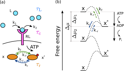
Figure 1: The cell signaling network. (a) The time-varying ligand concentration is modeled as a Markovian signal with mean $\overline{L}$, variance $\sigma^{2}_{L}$ and correlation time ${\tau_{\rm L}}=\lambda^{-1}$. A free ligand molecule L (light blue circle) can bind at rate $k_{1}$ to a free receptor R (magenta protein) on the cell membrane (black line), forming the complex RL, and unbind at rate $k_{2}$ from RL. The correlation time of the receptor state is ${\tau_{\rm c}}$. The complex RL catalyzes the phosphorylation reaction, driven by ATP conversion, of a downstream readout from the unphosphorylated (inactive) state $x$ to the phosphorylated (active) state $x^{*}$, with rate $k_{\rm f}$. The phosphorylated readout then spontaneously decays to the $x$ state with rate $k_{\rm r}$. Microscopic reverse reactions of each signaling pathway are represented by dashed arrows. The relaxation time of the push-pull network is ${\tau_{\rm r}}$. (b) Free-energy landscape of a readout molecule across the activation/deactivation reactions. Fuel turnover, provided by ATP conversion, drives the activation (phosphorylation) reaction characterized by the forward rate $k_{\rm f}$ and its microscopic reverse rate $k_{\rm-f}$ (green arrows). Associated with this activation reaction is a free-energy drop $\Delta\mu_{1}=\log\frac{k_{\rm f}\overline{x}}{k_{-{\rm f}}\overline{x}^{*}}$. The deactivation pathway corresponds to the spontaneous release of the inorganic phosphate; it is characterized by the rate $k_{\rm r}$ and its microscopic reverse $k_{\rm-r}$ (blue arrows) and corresponds to a free-energy drop $\Delta\mu_{2}=\log\frac{k_{\rm r}\overline{x}^{*}}{k_{-{\rm r}}\overline{x}}$.

II.2 The cell sensing precision

Signal-to-noise ratio
The time-varying ligand concentration has a distribution of instantaneous values ${L}(t)$, and we would like to know how many of these the system can resolve. To this end we define the signal-to-noise ratio (SNR), see Fig. 2(a):

$$\text{SNR}\vcentcolon=\frac{\sigma^{2}_{{L}}}{(\delta\hat{{L}})^{2}}.$$ (3)

Here $\sigma^{2}_{{L}}$ is the variance of the ligand concentration ${L}(t)$; it is a measure for the total number of input states. The quantity $(\delta\hat{{L}})^{2}$ is the error in the estimate of the current ligand concentration. The signal-to-noise ratio thus quantifies the number of distinct ligand concentrations that the system can resolve. Since the system is stationary and time invariant, we can omit the argument in ${L}(t)$ and write ${L}={L}(t)$.

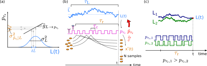
Figure 2: The precision of estimating a time-varying ligand concentration ${L}(t)$. (a) The cell estimates the current ligand concentration ${L}(t)$ by estimating the average receptor occupancy $p_{\tau_{\rm r}}$ over the past integration time ${\tau_{\rm r}}$ and by inverting the dynamic input-output relation $p_{\tau_{\rm r}}({L})$. The error in the estimate of the concentration $(\delta\hat{L})^{2}=\sigma^{2}_{{\hat{p}_{\tau_{r}}}|{L}}/\tilde{g}_{L\to p_{\tau_{\rm r}}}^{2}$ depends on the variance $\sigma^{2}_{\hat{p}_{\tau_{r}}|{L}}$ in the estimate of the average receptor occupancy $\hat{p}_{\tau_{r}}$ and the dynamic gain $\tilde{g}_{L\to p_{\tau_{\rm r}}}$, the slope of $p_{\tau_{\rm r}}({L})$, which determines how the error in $\hat{p}_{\tau_{r}}$ propagates to that in $\delta\hat{L}$. The input distribution has width $\sigma^{2}_{L}$. (b) The average receptor occupancy $p_{\tau_{\rm r}}$ over the past integration time ${\tau_{\rm r}}$ is estimated via the downstream network, which is modelled as a device that discretely samples the ligand-binding state of the receptor via its readout molecules $x$ Govern2014 ; the fraction of modified readout molecules provides an estimate of $p_{\tau_{\rm r}}$, see Eq. 7. The sensing error has two contributions, Eq. 20: the sampling error and the dynamical error. The sampling error arises from the error in the estimate of $p_{\tau_{\rm r}}$ that is due to the stochasticity of the sampling process; it depends on the number of samples, their independence and their accuracy. (c) The dynamical error arises because the current ligand concentration ${L}(t)$ is estimated via the average receptor occupancy $p_{\tau_{\rm r}}$ over the past integration time ${\tau_{\rm r}}$: the latter depends on the ligand concentration in the past ${\tau_{\rm r}}$, which will, in general, deviate from the current concentration. Two different input trajectories ($L_{1}$ in blue, $L_{2}$ in green) ending at time $t$ at the same value ${L}(t)$ (red dot) lead to different estimates of ${L}(t)$, due to their different average receptor occupancy ($p_{{\tau_{\rm r}},1}>p_{{\tau_{\rm r}},2}$) in the past ${\tau_{\rm r}}$.

Inferring concentration from readout
The cell estimates the current ligand concentration ${L}(t)$ from the instantaneous number of active readout molecules $x^{*}(t)$. In the Gaussian model employed here, we can calculate the SNR defined by Eq. 3, and it is related to the mutual information $I(x^{*};{L})=1/2\ln(1+{\rm SNR})$ between the input ${L}$ and the output $x^{*}$ (section S-II SI). However, the resulting expression for the SNR is not very instructive (Eq. S21):

$${\rm SNR}^{-1} =\frac{(\lambda+\mu)^{2}(\lambda+\mu^{\prime})^{2}}{\rho^{2}\rho^{\prime^{2}}\sigma^{2}_{L}}f(1-f)X_{\rm T}$$

$$+\frac{(\lambda+\mu)^{2}(\lambda+\mu^{\prime})^{2}}{\sigma^{2}_{L}\mu^{\prime}(\mu+\mu^{\prime})\rho^{2}}p(1-p)R_{\rm T}$$

$$+\frac{(\lambda+\mu)(\lambda+\mu^{\prime})(\lambda+\mu+\mu^{\prime})}{\mu\mu^{\prime}(\mu+\mu^{\prime})}-1.$$ (4)

This approach cannot elucidate the design logic of the system, because it treats the signal transmission from the input ${L}$ to the output $x^{*}$ as a black box. The central quantity in this calculation is the covariance $\sigma^{2}_{{L},x^{*}}$ between the ligand ${L}(t)$ and the readout $x^{*}(t)$ (see section S-II), which does not reveal how the signal is relayed from the input to the output. To elucidate the system’s design principles, we have to open the black box: we need to recognize that the input signal is transmitted to the output via the receptor, and that the cell does not estimate the ligand concentration from $x^{*}$ directly, but rather via its receptor (see Fig. 1). We can indeed arrive at a much more illuminating form of the same result as Eq. 4 by starting from the notion that the cell uses its readout system to estimate the receptor occupancy, from which the ligand concentration is then inferred. However, to develop this notion into a theory, we need new concepts, which we describe next.

Inferring concentration from receptor occupancy
The central idea of our theory is illustrated in Fig. 2a: the cell employs the push-pull network to estimate the average receptor occupancy $p_{\tau_{\rm r}}$ over the past integration time ${\tau_{\rm r}}$, and then uses this estimate ${\hat{p}_{{\tau_{r}|{L}}}}$ to infer the current concentration ${L}$ by inverting the mapping $p_{\tau_{\rm r}}({L})$. The sensing error is then determined by how accurately the cell estimates $p_{\tau_{\rm r}}$ and how the error in ${\hat{p}_{{\tau_{r}|{L}}}}$ propagates to that in ${L}$, which is determined by $p_{\tau_{\rm r}}({L})$. We now first give an overview of the central concepts.

Dynamic input-output relation The mapping $p_{\tau_{\rm r}}({L})$ is the dynamic input-output relation. It gives the average receptor occupancy over the past integration time ${\tau_{\rm r}}$ given that the current value of the input signal is ${L}={L}(t)$, see Fig. 2(a). Here, the average is not only over the noise in receptor-ligand binding and readout activation (Fig. 2(b)), but also over the subensemble of past input trajectories that each end at the same current concentration ${L}$ (Fig. 2(c)) Tostevin2010 ; Hilfinger:2011ev ; Bowsher2013 . In contrast to the conventional, static input-output relation $p({L}_{\rm s})$, which gives the average receptor occupancy $p$ for a steady-state ligand concentration ${L}_{\rm s}$ that does not vary in time, the dynamic input-output relation takes into account the dynamics of the input signal and the finite response time of the system. It depends on all the timescales in the problem: the timescale of the input, ${\tau_{\rm L}}$, the receptor-ligand correlation time ${\tau_{\rm c}}$, and the integration time ${\tau_{\rm r}}$. Only when ${\tau_{\rm L}}\gg{\tau_{\rm c}},{\tau_{\rm r}}$, does the dynamic input-output relation $p_{\tau_{\rm r}}({L})$ become equal to the static input-output relation $p({L}_{\rm s})$.

Sensing error Linearizing the dynamic input-output relation $p_{\tau_{\rm r}}({L})$ around the mean ligand concentration $\overline{{L}}$ (see Fig. 2a) and using the rules of error propagation, the expected error in the concentration estimate is then

$$(\delta\hat{{L}})^{2}=\frac{\sigma^{2}_{{\hat{p}_{{\tau_{r}|{L}}}}}}{\tilde{g}_{L\to p_{\tau_{\rm r}}}^{2}}.$$ (5)

Here $\sigma^{2}_{\hat{p}_{\tau_{r}}|{L}}$ is the variance in the estimate ${\hat{p}_{{\tau_{r}|{L}}}}$ of the average receptor occupancy over the past ${\tau_{\rm r}}$ given that the current input signal is ${L}$, see Fig. 2(a). The quantity $\tilde{g}_{L\to p_{\tau_{\rm r}}}$ is the dynamic gain, which is the slope of the dynamic input-output relation $p_{\tau_{\rm r}}({L})$; it determines how much an error in the estimate of $p_{\tau_{\rm r}}$ propagates to that in ${L}$. Eq. 5 generalizes the expression for the error in sensing static concentrations Berg:1977bp ; Bialek2005 ; Wang2007 ; Mehta2012 ; Kaizu2014 ; Govern2014 ; tenWolde:2016ih to that of time-varying concentrations.

SNR Combining Eqs. 5 and 3 yields the signal-to-noise ratio:

$$\text{SNR}=\frac{\tilde{g}^{2}_{{L}\to p_{{\tau_{\rm r}}}}}{\sigma^{2}_{{\hat{p}_{{\tau_{r}|{L}}}}}}\;\sigma^{2}_{{L}}.$$ (6)

Estimating the receptor occupancy To derive the error in estimating $p_{\tau_{\rm r}}$, $\sigma^{2}_{\hat{p}_{{\tau_{r}|{L}}}}$, we view, following our earlier work Govern2014 , the push-pull network as a device that discretely samples the receptor state (see Fig. 2(b)). The principle is that cells employ the activation reaction ${x+RL\to x^{*}+RL}$ to store the state of the receptor in stable chemical modification states of the readout molecules. Readout molecules that collide with a ligand-bound receptor are modified, while those that collide with an unbound receptor are not (Fig. 2(b)). The readout molecules serve as samples of the receptor at the time they were created, and collectively they encode the history of the receptor. The average receptor occupancy $p_{\tau_{\rm r}}$ over the past integration time ${\tau_{\rm r}}$ is thus estimated from the current number of active readout molecules $x^{*}({L}(t))=x^{*}(L)$:

$${\hat{p}_{{\tau_{r}|{L}}}}=\frac{x^{*}(L)}{\overline{N}},$$ (7)

where $\overline{N}$ is the average number of samples obtained during ${\tau_{\rm r}}$. To determine the effective number of independent samples, we need to consider not only the creation of the samples, but also their decay and accuracy. Samples decay via the deactivation reaction ${x^{*}\to x}$, which means that they only provide information on the receptor occupancy over the past ${\tau_{\rm r}}$. In addition, both the activation and the deactivation reaction can happen in their microscopic reverse direction, which corrupts the coding. Energy is needed to break time reversibility and protect the coding. Furthermore, for time-varying signals, we also need to recognize that the samples correspond to the ligand concentration over the past integration time ${\tau_{\rm r}}$, which will in general differ from the current concentration ${L}$ that the cell aims to estimate. While a finite ${\tau_{\rm r}}$ is necessary for time integration, it will also lead to a systematic error in the estimate of the concentration that the cell cannot reduce by taking more receptor samples.

Estimating concentration from ${\bm{p}_{\tau_{\rm r}}}$ is no different from that via readout ${\bm{x}^{*}}$ Because the average number of samples $\overline{N}$ is a constant, it follows from Eq. 7 that the variance in $x^{*}$ given an input ${L}$ is $\sigma^{2}_{x^{*}|{L}}=\sigma^{2}_{{\hat{p}_{{\tau_{r}|{L}}}}}\overline{N}^{2}$ while the gain from ${L}$ to $x^{*}$ is $\tilde{g}^{2}_{{L}\to x^{*}}=\tilde{g}^{2}_{{L}\to p_{\tau_{\rm r}}}\overline{N}^{2}$. Consequently, the absolute error $(\delta\hat{L})^{2}$ in estimating the concentration via $x^{*}$, $(\delta\hat{L})^{2}=\sigma^{2}_{x^{*}|{L}}/\tilde{g}^{2}_{{L}\to x^{*}}$, is the same as that of Eq. 5 : because the instantaneous number of active readout molecules $x^{*}$ reflects the average receptor occupancy $p_{\tau_{\rm r}}$ over the past ${\tau_{\rm r}}$, estimating the ligand concentration from $x^{*}$ is no different from inferring it from the average receptor occupancy ${\hat{p}_{{\tau_{r}|{L}}}}=x^{*}/\overline{N}$. In the Supporting Information we show explicitly that the central result of our manuscript that follows from the sampling framework, Eq. 20, is indeed identical to that of Eq. 4 (section S-IV).

Key steps derivation central result We now sketch the derivation of the central result for a simpler system, the irreversible network ($k_{\rm-f}=k_{\rm-r}=0$). For details and the result on the full system, see SI.

Dynamic gain The dynamic gain $\tilde{g}_{L\to p_{\tau_{\rm r}}}=\delta p_{\tau_{\rm r}}/\delta{L}(t)$ quantifies the mapping between the deviation $\delta{L}(t)\equiv{L}(t)-\overline{{L}}$ of the current ligand concentration ${L}(t)$ from its mean $\overline{{L}}$ and the deviation $\delta p_{\tau_{\rm r}}$ of the average receptor occupancy over the past integration time ${\tau_{\rm r}}$ from its mean $p$, see Fig. 2(a). This average is taken by the readout molecules at time $t$. Taking into account deactivation, the probability that a readout molecule at time $t$ provides a sample of the receptor at an earlier time $t_{i}$ is $p(t_{i}|{\rm sample})=e^{-(t-t_{i})/{\tau_{\rm r}}}/{\tau_{\rm r}}$ Govern2014 . Averaging the receptor occupancy over the sampling times $t_{i}$ then yields

$$\delta p_{\tau_{\rm r}}=\int_{-\infty}^{t}dt_{i}\langle\delta n(t_{i})\rangle_{\delta{L}(t)}\frac{e^{-(t-t_{i})/{\tau_{\rm r}}}}{{\tau_{\rm r}}}.$$ (8)

Here, $\langle\delta n(t_{i})\rangle_{\delta{L}(t)}=\langle n(t_{i})\rangle_{\delta{L}(t)}-p$ is the average deviation in the receptor occupancy $n(t_{i})=0,1$ at time $t_{i}$ given that the ligand concentration at time $t$ is $\delta{L}(t)$, where the average is taken over receptor-ligand binding noise and the subensemble of ligand trajectories that each end at $\delta{L}(t)$ (see Fig. 2c). We can compute it within the linear-noise approximation:

$$\langle\delta n(t_{i})\rangle_{\delta{L}(t)}=\rho_{n}\int_{-\infty}^{t_{i}}dt^{\prime}\langle\delta{L}(t^{\prime})\rangle_{\delta{L}(t)}e^{-(t_{i}-t^{\prime})/{\tau_{\rm c}}},$$ (9)

where $\rho_{n}=p(1-p)/(\overline{L}_{T}{\tau_{\rm c}})$ and $\langle\delta{L}(t^{\prime})\rangle_{\delta{L}(t)}$ is the average ligand concentration at time $t^{\prime}$ given that the concentration at time $t$ is $\delta{L}(t)$. It is given by Bowsher2013

$$\langle\delta{L}(t^{\prime})\rangle_{\delta{L}(t)}=\delta{L}(t)e^{-|t-t^{\prime}|/{\tau_{\rm L}}}.$$ (10)

Combining Eqs. 8-10 yields

$$\tilde{g}_{L\to p_{\tau_{\rm r}}} =\frac{p(1-p)}{\overline{L}}\left(1+\frac{{\tau_{\rm c}}}{{\tau_{\rm L}}}\right)^{-1}\left(1+\frac{{\tau_{\rm r}}}{{\tau_{\rm L}}}\right)^{-1},$$ (11)

$$=g_{{L}\to p}\left(1+\frac{{\tau_{\rm c}}}{{\tau_{\rm L}}}\right)^{-1}\left(1+\frac{{\tau_{\rm r}}}{{\tau_{\rm L}}}\right)^{-1}.$$ (12)

The dynamic gain $\tilde{g}_{L\to p_{\tau_{\rm r}}}$ depends on all the timescales in the problem. Only when ${\tau_{\rm L}}\gg{\tau_{\rm r}},{\tau_{\rm c}}$ is the average ligand concentration over the subensemble of trajectories ending at $\delta{L}(t)$ equal to current concentration $\delta{L}(t)$ (see Fig. 2(c)), and does $\tilde{g}_{L\to p_{\tau_{\rm r}}}$ become equal to its maximal value, the static gain $g_{{L}\to p}=p(1-p)/\overline{L}$.

The error in estimating the receptor occupancy Using the law of total variance, the error $\sigma^{2}_{\hat{p}_{\tau_{r}}|{L}}$ in the estimate of the receptor occupancy $p_{\tau_{\rm r}}$ over the past integration time ${\tau_{\rm r}}$ is given by

$$\sigma_{\hat{p}_{\tau_{r}}|{L}}^{2}=\text{var}\left[E({\hat{p}_{{\tau_{r}|{L}}}}|N)\right]+E\left[\text{var}({\hat{p}_{{\tau_{r}|{L}}}}|N)\right].$$ (13)

The first term reflects the variance of the mean of ${\hat{p}_{{\tau_{r}|{L}}}}$ given the number of samples $N$; the second term reflects the mean of the variance in ${\hat{p}_{{\tau_{r}|{L}}}}$ given the number of samples $N$ Govern2014 .

The first term of Eq. 13 is given by (see Eq. S48)

$$\text{var}\left[E({\hat{p}_{{\tau_{r}|{L}}}}|N)\right]=\frac{p^{2}}{\overline{N}}.$$ (14)

This contribution reflects the fact that with a push-pull network as considered here, the cell cannot discriminate between those readout molecules that have collided with an unbound receptor, and hence provide a sample of the receptor, and those that have not collided with a receptor at all; this term is zero for a bifunctional kinase where the unbound receptor catalyzes readout deactivation Govern2014 .

The second term of Eq. 13 contains two contributions. First we note that (Eq. S50 and Appendix S-B)

$${\rm var}\left(\frac{\sum_{i=1}^{N}n_{i}(t_{i})}{N}|N\right)$$

$$=\frac{p(1-p)}{N}+\overline{E\langle\delta n_{i}(t_{i})\delta n_{j}(t_{j})\rangle}_{\delta{L}(t)}-\tilde{g}^{2}\sigma^{2}_{L},$$ (15)

where $\delta n_{i}(t_{i})=n_{i}(t_{i})-p$, $E$ denotes an average over the sampling times $t_{i}$, and the overline an average over $\delta{L}$. The receptor covariance $\overline{E\langle\delta n_{i}(t_{i})\delta n_{j}(t_{j})\rangle}_{\delta{L}(t)}$ can be decomposed into two contributions. The first combines with the first term of Eq. 15 to yield (Eq. S61)

$$E\left[\text{var}({\hat{p}_{{\tau_{r}|{L}}}}|N)\right]^{\rm samp}=\frac{p(1-p)}{\overline{N}_{\rm I}},$$ (16)

where $\overline{N}_{\rm I}=f_{I}\overline{N}$. Here, $f_{I}=1/(1+2{\tau_{\rm c}}/\Delta)$, with ${\tau_{\rm c}}$ the receptor-ligand correlation time and $\Delta$ the spacing between the receptor samples, is the fraction of the $\overline{N}$ samples that are independent. Eq. 16 is the error in the estimate of the receptor occupancy based on a single measurement—the variance of the receptor occupancy $p(1-p)$—divided by the total number of independent measurements, $\overline{N}_{\rm I}=f_{I}\overline{N}$. Together with the first term of Eq. 13 (i.e. Eq. 14) Eq. 16 yields the sampling error in the estimate of the average receptor occupancy over ${\tau_{\rm r}}$:

$$\sigma^{2,\,\,{\rm samp}}_{{\hat{p}_{{\tau_{r}|{L}}}}}=\frac{p^{2}}{\overline{N}}+\frac{p(1-p)}{\overline{N}_{\rm I}}.$$ (17)

Both contributions to $\sigma^{2,\,\,{\rm samp}}_{{\hat{p}_{{\tau_{r}|{L}}}}}$ are governed by the nature of the receptor sampling process and do not depend on the input statistics. They are indeed the same as those for sensing static concentrations, derived previously Govern2014 .

The second contribution to Eq. 13 comes from the second contribution to $\overline{E\langle\delta n_{i}(t_{i})\delta n_{j}(t_{j})\rangle}_{\delta{L}(t)}$ in Eq. 15. It combines with the third term of Eq. 15 to yield (see Eq. S72)

$$\sigma^{2,\,\,{\rm dyn}}_{{\hat{p}_{{\tau_{r}|{L}}}}} =E\left[\text{var}({\hat{p}_{{\tau_{r}|{L}}}}|N)\right]^{\rm dyn}$$

$$=\tilde{g}^{2}\sigma^{2}_{L}\left[\left(1+\frac{{\tau_{\rm c}}}{{\tau_{\rm L}}}\right)\left(1+\frac{{\tau_{\rm r}}}{{\tau_{\rm L}}}\right)\left(1+\frac{{\tau_{\rm c}}{\tau_{\rm r}}}{{\tau_{\rm L}}({\tau_{\rm c}}+{\tau_{\rm r}})}\right)-1\right]$$ (18)

This is the dynamical error in estimating $p_{\tau_{\rm r}}$. It corresponds to the variation in $p_{\tau_{\rm r}}$ that arises from the different concentration trajectories in the past ${\tau_{\rm r}}$ that each end at $\delta{L}(t)$, see Fig. 2(c). This error does depend on the statistics of the input signal: it increases with the width of the input distribution, $\sigma^{2}_{L}$, and decreases with the input timescale ${\tau_{\rm L}}$.

The error in estimating the average receptor occupancy $p_{\tau_{\rm r}}$ is then given by

$$\sigma^{2}_{{\hat{p}_{{\tau_{r}|{L}}}}}=\sigma^{2,\,\,{\rm samp}}_{{\hat{p}_{{\tau_{r}|{L}}}}}+\sigma^{2,\,\,{\rm dyn}}_{{\hat{p}_{{\tau_{r}|{L}}}}},$$ (19)

where $\sigma^{2,\,\,{\rm samp}}_{{\hat{p}_{{\tau_{r}|{L}}}}}$ and $\sigma^{2,\,\,{\rm dyn}}_{{\hat{p}_{{\tau_{r}|{L}}}}}$ are given by Eqs. 17 and 18.

Central result To know how the error $\sigma^{2}_{{\hat{p}_{{\tau_{r}|{L}}}}}$ in the estimate of the average receptor occupancy $p_{\tau_{\rm r}}$ propagates to the error $(\delta\hat{L})^{2}$ in the estimate of the ligand concentration, we divide Eq. 19 by the dynamic gain $\tilde{g}_{L\to p_{\tau_{\rm r}}}$ given by Eq. 11 (see Eq. 6). For the full system, the reversible push-pull network, this yields the central result of our manuscript, the signal-to-noise ratio in terms of the total number of receptor samples, their independence, their accuracy, and the timescale on which they are generated:

$$\text{SNR}^{-1} = \underbrace{\left(1+\frac{{\tau_{\rm c}}}{{\tau_{\rm L}}}\right)^{2}\left(1+\frac{{\tau_{\rm r}}}{{\tau_{\rm L}}}\right)^{2}\left[\frac{\left(\overline{{L}}/\sigma_{L}\right)^{2}}{p(1-p)\overline{N}_{\rm I}}+\frac{\left(\overline{{L}}/\sigma_{L}\right)^{2}}{(1-p)^{2}\overline{N}_{\rm eff}}\right]}_{\text{sampling error}}+\underbrace{\left(1+\frac{{\tau_{\rm c}}}{{\tau_{\rm L}}}\right)\left(1+\frac{{\tau_{\rm r}}}{{\tau_{\rm L}}}\right)\left(1+\frac{{\tau_{\rm c}}{\tau_{\rm r}}}{{\tau_{\rm L}}({\tau_{\rm c}}+{\tau_{\rm r}})}\right)-1}_{\text{dynamical error}}.$$ (20)

This expression represents exactly the same result as that obtained by the straightforward linear-noise calculation, Eq. 4 (section S-IV). However, it is much more illuminating. It shows that the sensing error ${\rm SNR}^{-1}$ can be decomposed into two distinct contributions, which each have a clear interpretation: the sampling error, arising from the stochasticity in the sampling of the receptor state, and the dynamical error, arising from the dynamics of the input signal.

When the timescale of the ligand fluctuations ${\tau_{\rm L}}$ is much longer than the receptor correlation time ${\tau_{\rm c}}$ and the integration time ${\tau_{\rm r}}$, ${\tau_{\rm L}}\gg{\tau_{\rm r}},{\tau_{\rm c}}$, the dynamical error reduces to zero and only the sampling error remains. In this limit, the prefactor $(1+{\tau_{\rm c}}/{\tau_{\rm L}})^{2}(1+{\tau_{\rm r}}/{\tau_{\rm L}})^{2}$ becomes unity, and the relative sensing error $(\delta\hat{{L}}/\overline{{L}})^{2}$ (instead of ${\rm SNR}^{-1}=(\delta\hat{{L}}/\sigma_{L})^{2}$) reduces to that of estimating static concentrations, derived previously in Ref. Govern2014 . Here, $\overline{N}_{\rm eff}$ is the total number of effective samples and $\overline{N}_{\rm I}$ is the number of these that are independent Govern2014 . For the full system they are given by:

$$\overline{N}_{\rm I}=\underbrace{\frac{1}{(1+2\tau_{c}/\Delta)}}_{f_{I}}\underbrace{\overbrace{\frac{\left(e^{\beta\Delta\mu_{1}}-1\right)\left(e^{\beta\Delta\mu_{2}}-1\right)}{e^{\beta\Delta\mu}-1}}^{q}\overbrace{\frac{\dot{n}\tau_{r}}{p}}^{\bar{N}}}_{\bar{N}_{\rm eff}}.$$ (21)

The quantity $\dot{n}=k_{\rm f}pR_{\rm T}\overline{x}-k_{-{\rm f}}pR_{\rm T}\overline{x}^{*}$ is the net flux of $x$ around the cycle of activation and deactivation. It equals the rate at which $x$ is modified by the ligand-bound receptor; the quantity $\dot{n}/p$ is thus the sampling rate of the receptor, be it ligand bound or not. Multiplied with the relaxation rate ${\tau_{\rm r}}$, it yields the total number of receptor samples $\overline{N}$ obtained during ${\tau_{\rm r}}$. However, not all these samples are reliable. The effective number of samples is $\overline{N}_{\rm eff}=q\overline{N}$, where $0<q<1$ quantifies the quality of the sample. Here, $\beta=1/(k_{\rm B}T)$ is the inverse temperature, $\Delta\mu_{1}$ and $\Delta\mu_{2}$ are the free-energy drops over the activation and deactivation reaction, respectively, with $\Delta\mu=\Delta\mu_{1}+\Delta\mu_{2}$ the total drop, determined by the fuel turnover (see Fig. 1(b)). If the system is in thermodynamic equilibrium, $\Delta\mu_{1}=\Delta\mu_{2}=\Delta\mu=0$, $q\to 0$ and the system cannot sense, while if the system is strongly driven and $\Delta\mu_{1},\Delta\mu_{2}\to\infty$, $q\to 1$ and $\overline{N}_{\rm eff}\to\overline{N}$. Yet, even when all samples are reliable, they may contain redundant information on the receptor state. The factor $f_{\rm I}$ is the fraction of the $\overline{N}_{\rm eff}$ samples that are independent. It reaches unity when the receptor sampling interval $\Delta=2{\tau_{\rm r}}/(\overline{N}_{\rm eff}/R_{\rm T})$ becomes larger than the receptor correlation time ${\tau_{\rm c}}$.

When the number of samples becomes very large and $\overline{N}_{\rm I},\overline{N}_{\rm eff}\to\infty$, the sampling error reduces to zero. However, the sensing error still contains a second contribution, which, following Ref. Bowsher2013 , we call the dynamical error. This contribution only depends on timescales. It arises from the fact that the samples encode the receptor history and hence the ligand concentration over the past ${\tau_{\rm r}}$, which will, in general, deviate from the quantity that the cell aims to predict—the current concentration ${L}$. Indeed, this contribution yields a systematic error, which cannot be eliminated by increasing the number of receptor samples, their independence or their accuracy. It can only be reduced to zero by making the integration time ${\tau_{\rm r}}$ much smaller than the ligand timescale ${\tau_{\rm L}}$ (assuming that ${\tau_{\rm c}}$ is typically much smaller than ${\tau_{\rm r}},{\tau_{\rm L}}$). Only in this regime will the ligand concentration in the past ${\tau_{\rm r}}$ be similar to the current concentration, and can the latter be reliably inferred from the occupancy of the receptor provided the latter has been estimated accurately by taking enough samples.

Importantly, the dynamics of the input signal not only affects the sensing precision via the dynamical error, but also via the sampling error. This effect is contained in the prefactor of the sampling error, $(1+{\tau_{\rm c}}/{\tau_{\rm L}})^{2}(1+{\tau_{\rm r}}/{\tau_{\rm L}})^{2}$, which has its origin in the dynamic gain $\tilde{g}_{L\to p_{\tau_{\rm r}}}$ (Eq. 11). It determines how the sampling error $\sigma^{2,\rm samp}_{\hat{p}_{{\tau_{r}|{L}}}}$ in the estimate of $p_{\tau_{\rm r}}$ (Eq. 17) propagates to the error in the estimate of ${L}$ (see Eq. 6). Only when ${\tau_{\rm c}},{\tau_{\rm r}}\ll{\tau_{\rm L}}$ can the readout system closely track the input signal, and does $\tilde{g}_{L\to p_{\tau_{\rm r}}}$ reach its maximal value, the static gain ${g_{L\to p}}$, thus minimizing the error propagation from $p_{\tau_{\rm r}}$ to ${L}$.

III Fundamental resources

We can use Eq. 20 to identify the fundamental resources for cell sensing Govern2014 . A fundamental resource is a (collective) variable $Q_{i}$ that, when fixed to a constant, puts a non-zero lower bound on $\text{SNR}^{-1}$, no matter how the other variables are varied. It is thus mathematically defined as:

$${\rm MIN}_{Q_{i}={\rm const}}\left(\text{SNR}^{-1}\right)=f({\rm const})>0.$$ (22)

To find these collective variables, we numerically or analytically minimized $\text{SNR}^{-1}$, constraining (combinations of) variables yet optimizing over the other variables. To this end, it is helpful to rewrite Eq. 20 by splitting the first term in between the square brackets of the sampling error and then grouping one term with the second term using that $\overline{N}_{\rm eff}=q\overline{N}=q\dot{n}{\tau_{\rm r}}/p$ (see also section S-V):

$$\text{SNR}^{-1} =\left(1+\frac{{\tau_{\rm c}}}{{\tau_{\rm L}}}\right)^{2}\left(1+\frac{{\tau_{\rm r}}}{{\tau_{\rm L}}}\right)^{2}\left[\underbrace{\frac{\left(\overline{{L}}/\sigma_{L}\right)^{2}}{p(1-p)R_{\rm T}(1+{\tau_{\rm r}}/{\tau_{\rm c}})}}_{\text{receptor input noise}}+\underbrace{\frac{\left(\overline{{L}}/\sigma_{L}\right)^{2}}{(1-p)^{2}q\dot{n}{\tau_{\rm r}}}}_{\text{coding noise}}\right]+\underbrace{\left(1+\frac{{\tau_{\rm c}}}{{\tau_{\rm L}}}\right)\left(1+\frac{{\tau_{\rm r}}}{{\tau_{\rm L}}}\right)\left(1+\frac{{\tau_{\rm c}}{\tau_{\rm r}}}{{\tau_{\rm L}}({\tau_{\rm c}}+{\tau_{\rm r}})}\right)-1}_{\text{dynamical error}}.$$ (23)

The first term in between the square brackets describes the contribution that comes from the stochasticity in the concentration measurements at the receptor level. The second term in between the square brackets, the coding noise, describes the error that arises in storing these measurements into the readout molecules.

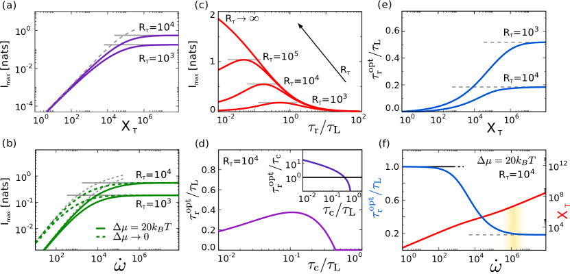
Figure 3: Receptors $R_{\rm T}$, readout molecules $X_{\rm T}$ and $\dot{w}$ fundamentally limit sensing, and there exists an optimal integration time ${\tau_{\rm r}}$ that depends on which of the resources is limiting. (a+b) $R_{\rm T}$, $X_{\rm T}$ and $\dot{w}$ are fundamental resources, with no trade-offs between them. Plotted is the maximum mutual information $I_{\rm max}=1/2\ln(1+{\rm SNR}_{\rm max})$, obtained by minimizing Eq. 23 over $p$ and ${\tau_{\rm r}}$, for different combinations of (a) $X_{\rm T}$ and $R_{\rm T}$ in the irreversible limit $q\to 1$, and (b) $\dot{w}$ and $R_{\rm T}$ for two different values of $\Delta\mu$. The sensing precision is bounded by the limiting resource, $R_{\rm T}$ (solid grey lines, Eq. 24), $X_{\rm T}$ (dashed grey line, Eq. 25, panel a), or $\dot{w}$ (dashed grey lines, Eqs. 27 and 28, panel b). (c) $I_{\rm max}$ as a function of ${\tau_{\rm r}}$ for different values of $R_{\rm T}$ in the Berg-Purcell limit ($q\to 1$ and $X_{\rm T}\to\infty$). There exists an optimal integration time ${\tau_{\rm r}}^{\rm opt}$ that maximizes the sensing precision; ${\tau_{\rm r}}^{\rm opt}$ decreases with $R_{\rm T}$. (d) In this limit, ${\tau_{\rm r}}^{\rm opt}$ depends non-monotonically on the receptor-ligand correlation time ${\tau_{\rm c}}$: it first increases with ${\tau_{\rm c}}$ to sustain time-averaging, but then drops when ${\tau_{\rm r}}^{\rm opt}/{\tau_{\rm c}}$ becomes of order unity and time-averaging is no longer effective (see inset). (e) ${\tau_{\rm r}}^{\rm opt}$ as a function of $X_{\rm T}$ for different values of $R_{\rm T}$. When $X_{\rm T}<R_{\rm T}$, time averaging is not possible and the optimal system is an instantaneous responder, ${\tau_{\rm r}}^{\rm opt}\to 0$; when $X_{\rm T}\gg R_{\rm T}$ the system reaches the Berg-Purcell regime in which $I_{\rm max}$ is limited by $R_{\rm T}$ rather than $X_{\rm T}$ (see panel a). (f) ${\tau_{\rm r}}^{\rm opt}$ and $X_{\rm T}$ as a function of $\dot{w}$. When the power $\dot{w}\sim X_{\rm T}/{\tau_{\rm r}}$ is limiting, the sampling error dominates and ${\tau_{\rm r}}^{\rm opt}$ equals ${\tau_{\rm L}}$ to maximize $X_{\rm T}$, minimizing the sampling error; ${\tau_{\rm r}}^{\rm opt}$ then decreases to trade part of the decrease in the sampling error for a reduction in the dynamical error such that both decrease; when the sampling interval $\Delta\sim{\tau_{\rm r}}R_{\rm T}/X_{\rm T}$ becomes comparable to ${\tau_{\rm c}}$, in the region marked by the yellow bar, the sampling error is no longer limited by $X_{\rm T}$, such that ${\tau_{\rm r}}$ now limits both sources of error; the two sources can therefore no longer be decreased simultaneously by increasing $\dot{w}\sim X_{\rm T}/{\tau_{\rm r}}$; the system has entered the Berg-Purcell regime where ${\tau_{\rm r}}^{\rm opt}$ is determined by $R_{\rm T}$ rather than $\dot{w}$ (see panel (b)). Parameter values unless specified: ${\tau_{\rm c}}/{\tau_{\rm L}}=10^{-2}$; $\sigma_{L}/\overline{L}_{T}=10^{-2}$.

Eq. 23 allows us to identify the fundamental resources by constraining combinations of variables while optimizing over others by taking limits (see Eq. 22). As we show below, this reveals that these resources are the number of receptors $R_{\rm T}$, their integration time ${\tau_{\rm r}}$, the number of readout molecules $X_{\rm T}$, and the power $\dot{w}=\dot{n}\Delta\mu$. Fig. 3 illustrates that these resources are indeed fundamental, and also elucidates the design logic of the system.

Panel (a) of Fig. 3 shows the maximal mutual information $I_{\rm max}(L;x^{*})$ as a function of $X_{\rm T}$ for different values of $R_{\rm T}$, obtained by optimizing Eq. 23 over $p$ and ${\tau_{\rm r}}$, in the irreversible limit $q\to 1$. When $X_{\rm T}$ is small, $I_{\max}$ cannot be increased by raising $R_{\rm T}$: no matter how many receptors the system has, the sensing precision is limited by the pool of readout molecules and only increasing this pool can raise $I_{\rm max}$. However, when $X_{\rm T}$ is large, $I_{\rm max}$ becomes independent of $X_{\rm T}$. In this regime, the number of receptors $R_{\rm T}$ limits the number of independent concentration measurements and only increasing $R_{\rm T}$ can raise $I_{\rm max}$. Similarly, panel (b) shows that when the power $\dot{w}$ is limiting, $I_{\rm max}$ cannot be increased by $R_{\rm T}$ but only by increasing $\dot{w}$. Clearly, the resources receptors, readout molecules and energy cannot compensate each other: the sensing precision is bounded by the limiting resource.

Importantly, however, while for sensing static concentrations the products $R_{\rm T}{\tau_{\rm r}}/{\tau_{\rm c}}$ (receptors and their integration time) and $\dot{w}{\tau_{\rm r}}$ (the energy) are fundamental Govern2014 , for time-varying signals $R_{\rm T}$, $\dot{w}$, and ${\tau_{\rm r}}$ separately limit sensing. Consequently, neither receptors $R_{\rm T}$ nor power $\dot{w}$ can be traded freely against time ${\tau_{\rm r}}$ to reach a desired sensing precision, as is possible for static signals. There exists an optimal integration time ${\tau_{\rm r}}^{\rm opt}$ that maximizes the sensing precision, and its value depends on which of the resources $R_{\rm T}$, $X_{\rm T}$ and $\dot{w}$ is limiting (Fig. 3(c)-(f)). We now discuss these three regimes in turn.

III.1 The number of receptors $R_{\rm T}$

As Berg and Purcell pointed out, cells can reduce the sensing error by increasing the number of receptors or by taking more measurements per receptor, via the mechanism of time integration Berg:1977bp . In the Berg-Purcell regime where the receptors and their integration time are limiting, the coding noise is zero and Eq. 23 reduces to

$$\text{SNR}^{-1} \geq\left(1+\frac{{\tau_{\rm r}}}{{\tau_{\rm L}}}\right)^{2}\frac{4\left(\overline{{L}}/\sigma_{L}\right)^{2}}{R_{\rm T}\;{\tau_{\rm r}}/{\tau_{\rm c}}}+\frac{{\tau_{\rm r}}}{{\tau_{\rm L}}}.$$ (24)

This result corresponds to the limits $X_{\rm T}\to\infty$ and $\dot{w}\to\infty$ in panels (a) and (b) of Fig. 3, respectively.

Eq. 24 shows that the sensing precision does not depend on $R_{\rm T}{\tau_{\rm r}}/{\tau_{\rm c}}$, as for static signals Govern2014 , but on $R_{\rm T}$ and ${\tau_{\rm r}}$ separately, such that an optimal integration time ${\tau_{\rm r}}^{\rm opt}$ emerges that maximizes the sensing precision (see Fig. 3c). Increasing ${\tau_{\rm r}}$ improves the mechanism of time integration by increasing the number of independent samples per receptor, ${\tau_{\rm r}}/{\tau_{\rm c}}$, thus reducing the sampling error (Eq. 20). However, increasing ${\tau_{\rm r}}$ raises the dynamical error. Moreover, it lowers the dynamical gain $\tilde{g}_{L\to p_{\tau_{\rm r}}}$, which increases the propagation of the error in the estimate of the receptor occupancy to that of the ligand concentration. The optimal integration time ${\tau_{\rm r}}^{\rm opt}$ arises as a trade-off between these three factors.

Fig. 3(c) also shows that the optimal integration time ${\tau_{\rm r}}^{\rm opt}$ decreases with the number of receptors $R_{\rm T}$. The total number of independent concentration measurements is the number of independent measurements per receptor, ${\tau_{\rm r}}/{\tau_{\rm c}}$, times the number $R_{\rm T}$ of receptors, $\overline{N}_{\rm I}=R_{\rm T}{\tau_{\rm r}}/{\tau_{\rm c}}$. As $R_{\rm T}$ increases, less measurements ${\tau_{\rm r}}/{\tau_{\rm c}}$ per receptor have to be taken to remove the receptor-ligand binding noise, explaining why ${\tau_{\rm r}}^{\rm opt}$ decreases as $R_{\rm T}$ increases. Indeed, the sensing error reduces to zero when $R_{\rm T}\to\infty$ and ${\tau_{\rm r}}\to 0$, allowing for optimal signal tracking.

Interestingly, ${\tau_{\rm r}}^{\rm opt}$ depends non-monotonically on the receptor-ligand correlation time ${\tau_{\rm c}}$ (Fig. 3d). When ${\tau_{\rm c}}$ increases at fixed ${\tau_{\rm r}}$, the receptor samples become more correlated. To keep the mechanism of time integration effective, ${\tau_{\rm r}}$ must increase as ${\tau_{\rm c}}$ rises. Increasing ${\tau_{\rm r}}$ will, however, also distort the signal, and to avoid too strong signal distortion the cell compromises on time integration by decreasing the ratio ${\tau_{\rm r}}/{\tau_{\rm c}}$ (see inset). When ${\tau_{\rm r}}$ becomes too large, the benefit of time integration no longer pays off the cost of signal distortion. Now not only the ratio ${\tau_{\rm r}}/{\tau_{\rm c}}$ decreases (inset of Fig. 3(d)), but also ${\tau_{\rm r}}$ itself (Fig. 3(c)). The sensing system switches to a different strategy. It no longer employs time integration, but rather becomes an instantaneous responder of the ligand-binding state of the receptor.

III.2 The number of readout molecules $X_{\rm T}$

To implement time integration, the cell needs to store the receptor states in the readout molecules. When the number of readout molecules $X_{\rm T}$ is limiting, the coding noise in Eq. 23 dominates over the receptor input noise. Noting that the flux $\dot{n}=f(1-f)qX_{\rm T}/{\tau_{\rm r}}$, with $f={\overline{x}^{*}/X_{\rm T}}$ the fraction of modified readout molecules, we find that in the irreversible regime ($q\to 1$), the sensing error is bounded by

$$\text{SNR}^{-1} \geq\left(1+\frac{{\tau_{\rm r}}}{{\tau_{\rm L}}}\right)^{2}\left[\frac{4\left(\overline{{L}}/\sigma_{L}\right)^{2}}{X_{\rm T}}\right]+\frac{{\tau_{\rm r}}}{{\tau_{\rm L}}}$$ (25)

$$\geq\frac{4\left(\overline{{L}}/\sigma_{L}\right)^{2}}{X_{\rm T}}.$$ (26)

Clearly, $X_{\rm T}$ is a fundamental resource that puts a hard bound on the mutual information (Fig. 3(a)).

Eqs. 25 and 26 show that to reach the sensing limit set by $X_{\rm T}$, the receptor integration time ${\tau_{\rm r}}$ needs to be zero. This is in marked contrast to the non-zero optimal integration ${\tau_{\rm r}}^{\rm opt}$ in the Berg-Purcell regime where $R_{\rm T}$ is limiting (see Fig. 3(c)). To elucidate this, Fig. 3(e) shows the optimal integration time ${\tau_{\rm r}}^{\rm opt}$ as a function of $X_{\rm T}$. When $X_{\rm T}$ is smaller than $R_{\rm T}$, the average number of samples per receptor is less than unity. At any given time, there are many receptors whose concentration measurements are not stored in the downstream readout molecules. In this regime, the system cannot time integrate the receptor, and to minimize signal distortion the optimal integration time ${\tau_{\rm r}}^{\rm opt}$ is essentially zero. However, when $X_{\rm T}$ is increased, the likelihood that two or more readout molecules provide a sample of the same receptor molecule rises, and time averaging becomes possible. Yet to obtain receptor samples that are independent, the integration time ${\tau_{\rm r}}$ must be increased to make the sampling interval $\Delta\sim{\tau_{\rm r}}R_{\rm T}/X_{\rm T}$ larger than the receptor correlation time ${\tau_{\rm c}}$. As $X_{\rm T}$ and hence the total number of samples $\overline{N}$ are increased further, the number of samples that are independent, $\overline{N}_{\rm I}$, only continues to rise when ${\tau_{\rm r}}$ increases with $X_{\rm T}$ further. However, while this reduces the sampling error, it does also increase the dynamical error. When the decrease in the sampling error no longer outweighs the increase in the dynamical error, ${\tau_{\rm r}}^{\rm opt}$ and the mutual information no longer change with $X_{\rm T}$ (see Fig. 3(a)). The system has entered the Berg-Purcell regime in which ${\tau_{\rm r}}^{\rm opt}$ and the mutual information are given by the optimization of Eq. 24 (grey dashed line). In this regime, increasing $X_{\rm T}$ merely adds redundant samples: the number of independent samples remains $\overline{N}_{\rm I}=R_{\rm T}{\tau_{\rm r}}^{\rm opt}/{\tau_{\rm c}}$.

III.3 The power $\dot{w}=\dot{n}\Delta\mu$

Time integration relies on copying the ligand-binding state of the receptor into the chemical modification states of the readout molecules Mehta2012 ; Govern2014 . This copy process correlates the state of the receptor with that of the readout, which requires work input Ouldridge:2017hs .

The free-energy $\Delta\mu$ provided by the fuel turnover drives the readout around the cycle of modification and demodification (Fig. 1). The rate at which the fuel molecules do work is the power $\dot{w}=\dot{n}\Delta\mu$ and the total work performed during the integration time ${\tau_{\rm r}}$ is $w\equiv\dot{w}{\tau_{\rm r}}$. This work is spent on taking samples of receptor molecules that are bound to ligand, because only they can modify the readout. The total number of effective samples of ligand-bound receptors during ${\tau_{\rm r}}$ is $p\overline{N}_{\rm eff}$ (Eq. 21), which means that the work per effective sample of a ligand-bound receptor is $w/(p\overline{N}_{\rm eff})=\Delta\mu/q$ Govern2014 .

To understand how energy limits the sensing precision, we can distinguish between two limiting regimes Govern2014 . When $\Delta\mu>4k_{\rm B}T$, the quality factor $q\to 1$ (Eq. 21) and the work per sample of a ligand-bound receptor is simply $w/(p\overline{N}_{\rm eff})=\Delta\mu$ Govern2014 . In this irreversible regime, the power limits the sensing accuracy not because it limits the reliability of each sample, but because it limits the rate $\dot{n}=\dot{w}/\Delta\mu$ at which the receptor is sampled:

$$\text{SNR}^{-1} \geq\left(1+\frac{{\tau_{\rm r}}}{{\tau_{\rm L}}}\right)^{2}\left(\frac{\Delta\mu\left(\overline{{L}}/\sigma_{L}\right)^{2}}{\dot{w}{\tau_{\rm r}}}\right)+\frac{{\tau_{\rm r}}}{{\tau_{\rm L}}},$$ (27)

obtained from Eq. 23 by taking $R_{\rm T}\to\infty$, $p\to 0$. This expression shows that the sensing precision is fundamentally bounded not by the work $w=\dot{w}{\tau_{\rm r}}$, as observed for static signals Govern2014 , but rather by the power $\dot{w}$ and the integration time ${\tau_{\rm r}}$ separately such that an optimal integration time ${\tau_{\rm r}}^{\rm opt}$ emerges (Fig. 3(f)).

When $\Delta\mu<4k_{\rm B}T$, the system enters the quasi-equilibrium regime in which the quality factor $q\to\beta\Delta\mu/4$ (see Eq. 21, noting that in the optimal system $\Delta\mu_{1}=\Delta\mu_{2}=\Delta\mu/2$) Govern2014 . The bound on the sensing error (Eq. 23) set by the power constraint now becomes

$$\text{SNR}^{-1} \geq\left(1+\frac{{\tau_{\rm r}}}{{\tau_{\rm L}}}\right)^{2}\left(\frac{4k_{\rm B}T\left(\overline{{L}}/\sigma_{L}\right)^{2}}{\dot{w}{\tau_{\rm r}}}\right)+\frac{{\tau_{\rm r}}}{{\tau_{\rm L}}}.$$ (28)

Comparing this expression to Eq. 27, which only holds when $\Delta\mu>4k_{\rm B}T$, it is clear that the sensing error is minimized in the quasi-equilibrium regime, see Fig. 3(b). This regime maximizes the number of effective measurements per work input, because the work per effective measurement reaches its fundamental lower bound, $w/(p\overline{N}_{\rm eff})=\Delta\mu/q=4k_{\rm B}T$ Govern2014 .

While the sensing precision for a given power and time constraint is higher in the quasi-reversible regime, more readout molecules are required to store the concentration measurements in this regime. Noting that the flux $\dot{n}=f(1-f)X_{\rm T}q/{\tau_{\rm r}}=\dot{w}/\Delta\mu$ (Eq. S114), it follows that in the irreversible regime ($q\to 1$) the number of readout molecules consuming energy at a rate $\dot{w}$ is

$$X_{\rm T}^{\rm irr}=\frac{\dot{w}{\tau_{\rm r}}}{\Delta\mu f(1-f)}$$ (29)

while in the quasi-equilibrium regime ($q\to\Delta\mu/4$) it is

$$X_{\rm T}^{\rm qeq}=\frac{\dot{w}{\tau_{\rm r}}4k_{\rm B}T}{\Delta\mu^{2}f(1-f)}.$$ (30)

Since in the quasi-equilibrium regime $\Delta\mu<4k_{\rm B}T$, $X_{\rm T}^{\rm qeq}>X_{\rm T}^{\rm irr}$.

Fig. 3(f) shows how the optimal integration time ${\tau_{\rm r}}^{\rm opt}$ depends on the power $\dot{w}$. Since the system cannot sense without any readout molecules, in the low power regime the system maximizes $X_{\rm T}$ subject to the power constraint $\dot{w}\sim X_{\rm T}/{\tau_{\rm r}}$ (see Eqs. 29 and 30) by making ${\tau_{\rm r}}$ as large as possible, which is the signal correlation time ${\tau_{\rm L}}$—increasing ${\tau_{\rm r}}^{\rm opt}$ further would average out the signal itself. As $\dot{w}$ is increased, $X_{\rm T}$ rises and the sampling error decreases. When the sampling error becomes comparable to the dynamical error (Eq. 20), the system starts to trade a further reduction in the sampling error for a reduction in the dynamical error: ${\tau_{\rm r}}^{\rm opt}$ now goes down. In this regime, the sampling error and the dynamical error are reduced simultaneously by increasing $X_{\rm T}$ and decreasing ${\tau_{\rm r}}^{\rm opt}$. This continues until the sampling interval $\Delta\sim R_{\rm T}{\tau_{\rm r}}/X_{\rm T}$ becomes comparable to the receptor correlation time ${\tau_{\rm c}}$, as marked by the yellow bar. Beyond this point, $\Delta<{\tau_{\rm c}}$ and the sampling error is no longer limited by $X_{\rm T}$ but rather by ${\tau_{\rm r}}$, since ${\tau_{\rm r}}$ bounds the number of independent samples per receptor, ${\tau_{\rm r}}/{\tau_{\rm c}}$. Because ${\tau_{\rm r}}$ now limits both sources of error, they can no longer be reduced simultaneously. The system has entered the Berg-Purcell regime, where ${\tau_{\rm r}}^{\rm opt}$ is determined by the trade-off between the dynamical error and the sampling error as set by the maximum number of independent samples, $R_{\rm T}{\tau_{\rm r}}/{\tau_{\rm c}}$ (Fig. 3(c)).

IV The optimal allocation principle, revisited

In sensing static concentrations, there exists three fundamental classes of resources: receptors and their integration time $R_{\rm T}{\tau_{\rm r}}/{\tau_{\rm c}}$, readout molecules $X_{\rm T}$, and energy $\dot{w}{\tau_{\rm r}}$ injected during ${\tau_{\rm r}}$ Govern2014 . These fundamental resource classes cannot compensate each other in achieving a desired sensing precision—they limit sensing like weak links in a chain. It means that in an optimally designed system each class is equally limiting so that no resource is wasted. This yields the design principle that in an optimal system $R_{\rm T}{\tau_{\rm r}}/{\tau_{\rm c}}\approx X_{\rm T}\approx\beta\dot{w}{\tau_{\rm r}}$ Govern2014 . However, in sensing time-varying signals, a trade-off between time integration and signal tracking is inevitable. As a result, besides $X_{\rm T}$, the receptors $R_{\rm T}$, the power $\dot{w}$ and the integration time ${\tau_{\rm r}}$ are each fundamental.

Can we nonetheless formulate a similar design principle? We cannot simply equate the bounds set by the number of receptors $R_{\rm T}$ and their integration time ${\tau_{\rm r}}$ (Eq. 24), the number of readout molecules $X_{\rm T}$ (Eq. 26) and the power $\dot{w}$ (Eq. 28), because they correspond to different sensing strategies: when $R_{\rm T}$ is limiting, there exists an optimal non-zero integration time ${\tau_{\rm r}}^{\rm opt}$, while if $X_{\rm T}$ is limiting ${\tau_{\rm r}}^{\rm opt}\approx 0$, as discussed above.

Remarkably, however, Eqs. 24,  25 and 28 have the same functional form $f(x)$, with $x=R_{\rm T}{\tau_{\rm r}}/{\tau_{\rm c}},X_{\rm T},\beta\dot{w}{\tau_{\rm r}}$, respectively. This means that when for a given ${\tau_{\rm r}}$, $R_{\rm T}{\tau_{\rm r}}/{\tau_{\rm c}}=X_{\rm T}=\beta\dot{w}{\tau_{\rm r}}$ and $f(R_{\rm T}{\tau_{\rm r}}/{\tau_{\rm c}})=f(X_{\rm T})=f(\beta\dot{w}{\tau_{\rm r}})$, the bounds on the sensing precision as set by, respectively, the number of receptors $R_{\rm T}$ (Eq. 24), the number of readout molecules $X_{\rm T}$ (Eq. 25), and the power $\dot{w}$ (Eq. 28), are equal. Each of these resources is now equally limiting sensing and no resource is in excess. We thus recover the optimal resource allocation principle originally formulated for systems sensing static concentrations Govern2014 :

$$R_{\rm T}{\tau_{\rm r}}/{\tau_{\rm c}}\approx X_{\rm T}\approx\beta\dot{w}{\tau_{\rm r}}.$$ (31)

Irrespective of whether the concentration fluctuates in time, the number of independent concentration measurements at the receptor level is $R_{\rm T}{\tau_{\rm r}}/{\tau_{\rm c}}$, which in an optimally designed system also equals the number of readout molecules $X_{\rm T}$ and the energy $\beta\dot{w}{\tau_{\rm r}}$ that are both necessary and sufficient to store these measurements reliably.

Importantly, Eq. 31 holds for any integration time ${\tau_{\rm r}}$, yet it does not specify ${\tau_{\rm r}}$. What is the optimal ${\tau_{\rm r}}$ that minimizes the sensing error? The design principle $R_{\rm T}{\tau_{\rm r}}/{\tau_{\rm c}}=X_{\rm T}$ means that for a fixed $X_{\rm T}$, $R_{\rm T}$ can be increased by simultaneously decreasing ${\tau_{\rm r}}$. This increases the sensing precision (see Fig. S1, S-VII). In fact, for a fixed $X_{\rm T}$, the precision is maximized when $R_{\rm T}=X_{\rm T}$ and ${\tau_{\rm r}}=0$, because in this limit the dynamical error is zero. However, the power diverges in this limit, because in the optimal system $\beta\dot{w}{\tau_{\rm r}}\approx X_{\rm T}$ (Eq. 31).

Intriguingly, the cell membrane is highly crowded and many systems employ time integration Berg:1977bp ; Bialek2005 ; Govern2014 . This suggests that these systems employ time integration and accept the signal distortion that comes with it, simply because there is not enough space on the membrane to increase $R_{\rm T}$. Our theory then allows us to predict the optimal integration time ${\tau_{\rm r}}^{\rm opt}$ based on the premise that $R_{\rm T}$ is limiting. As Eq. 24 reveals, in this limit ${\tau_{\rm r}}^{\rm opt}$ does not only depend on $R_{\rm T}$, but also on ${\tau_{\rm c}}$, ${\tau_{\rm L}}$, and $\sigma_{L}/\overline{{L}}$: ${\tau_{\rm r}}^{\rm opt}={\tau_{\rm r}}^{\rm opt}(R_{\rm T},{\tau_{\rm c}},{\tau_{\rm L}},\sigma_{{L}}/\overline{{L}})$. The optimal design of the system is then given by Eq. 31 but with ${\tau_{\rm r}}$ given by ${\tau_{\rm r}}^{\rm opt}={\tau_{\rm r}}^{\rm opt}(R_{\rm T},{\tau_{\rm c}},{\tau_{\rm L}},\sigma_{{L}}/\overline{{L}})$:

$$R_{\rm T}{\tau_{\rm r}}^{\rm opt}/{\tau_{\rm c}}\approx X_{\rm T}^{\rm opt}\approx\beta\dot{w}^{\rm opt}{\tau_{\rm r}}^{\rm opt}.$$ (32)

This design principle maximizes for a given number of receptors $R_{\rm T}$ the sensing precision, and minimizes the number of readout molecules $X_{\rm T}$ and power $\dot{w}$ needed to reach that precision.

V Comparison with experiments

If the number of receptors is limiting the sensing precision, then our theory predicts an optimal integration time ${\tau_{\rm r}}^{\rm opt}(R_{\rm T},{\tau_{\rm c}},{\tau_{\rm L}},\sigma_{{L}}/\overline{{L}})$ that is given by Eq. 24. We can test this prediction for the chemotaxis system of the bacterium E. coli, which has been well characterized experimentally. In this system, the receptor forms a complex with the kinase CheA. This complex, which can be coarse-grained into $R$ Govern2014 , can bind the ligand L and activate the intracellular messenger protein CheY ($x$) by phosphorylating it. Deactivation of CheY is catalyzed by CheZ, the effect of which can be coarse-grained into the deactivation rate. The E. coli chemotaxis system also exhibits adaptation on longer timescales, due to receptor methylation and demethylation. However, the integration time for the receptor-ligand binding noise is not given by the adaptation timescale, but rather by the relaxation rate of the push-pull network that controls CheY (de) phosphorylation Sartori:2011fh .

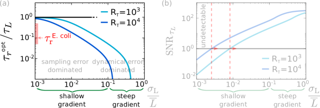
Figure 4: The optimal integration time for the chemotaxis system of E. coli. (a) The optimal integration time ${\tau_{\rm r}}^{\rm opt}$, obtained by numerically optimizing Eq. 24, as a function of the relative strength of the input noise, $\sigma_{L}/\overline{{L}}$, for two different copy numbers $R_{\rm T}$ of the receptor-CheA complexes; for an exponential gradient with length scale $x_{0}$, the relative noise strength $\sigma_{L}/\overline{{L}}\simeq l/x_{0}$, where $l\approx 50\mu{\rm m}$ is the run length of E. coli. It is seen that ${\tau_{\rm r}}^{\rm opt}$ increases as $\sigma_{L}/\overline{{L}}$ decreases. This is because the relative importance of the sampling error compared to the dynamical error increases, necessitating a longer integration time. The figure also shows that ${\tau_{\rm r}}^{\rm opt}$ decreases as $R_{\rm T}$ is increased, because that allows for more instantaneous measurements (see also Fig. 3). The red bar indicates the range of the estimated integration time of E. coli, $0.05{\rm ms}<{\tau_{\rm r}}<0.5{\rm ms}$, based on its attractant and repellent response respectively Sourjik2002 , divided by the input timescale ${\tau_{\rm L}}\approx 1{\rm s}$ based on its typical run time of about a second Berg:1972wt ; Taute:2015ce . The panel indicates that E. coli has been optimized to detect shallow concentration gradients. (b) The signal-to-noise ratio $\text{SNR}_{\tau_{\rm L}}=(\sigma_{L}/\delta\hat{{L}})^{2}{\tau_{\rm L}}/{\tau_{\rm r}}$ as a function of $\sigma_{L}/\overline{{L}}\simeq l/x_{0}$. To be able to detect the gradient, the $\text{SNR}_{\tau_{\rm L}}$ must exceed unity. The panel shows that the shallowest gradient that E. coli can detect (marked with dashed red line) has, for $R_{\rm T}=10^{4}$, a length scale of $x_{0}\approx 25000\mu{\rm m}$ (corresponding to $\sigma_{L}/\overline{{L}}\approx 2\times 10^{-3}$), which is consistent with experiments based on ramp responses Shimizu:2010ig . Other parameter: receptor-ligand binding correlation time ${\tau_{\rm c}}=10{\rm ms}$ Vaknin2007 ; Danielson1994 .

To test the prediction for ${\tau_{\rm r}}^{\rm opt}(R_{\rm T},{\tau_{\rm c}},{\tau_{\rm L}},\sigma_{{L}}/\overline{{L}})$, we need to estimate $R_{\rm T}$, ${\tau_{\rm c}}$, ${\tau_{\rm L}}$ and $\sigma_{{L}}/\overline{{L}}$. The number of receptor-CheA complexes depends on the growth rate and varies between $R_{\rm T}=10^{3}$ and $R_{\rm T}=10^{4}$ Li:2004eh . The dissociation constant for the binding of aspartate to the Tar receptor is $K_{D}\approx 0.1\mu{\rm M}$ Vaknin2007 , which with an association rate of $k_{\rm on}\approx 10^{9}{\rm M}^{-1}/{\rm s}$ Danielson1994 yields a receptor-ligand dissociation rate of $k_{\rm off}\approx 100{\rm s}^{-1}$. Protein occupancies are typically in the range $0.1-1$ and following our previous work we assume $p=0.5$ Govern2014 , which gives a receptor-ligand correlation time of ${\tau_{\rm c}}\simeq 1/(2k_{\rm off})\approx 10{\rm ms}$. The timescale ${\tau_{\rm L}}$ of the input fluctuations is set by the typical run time, which is on the order of a few seconds, ${\tau_{\rm L}}\approx 1{\rm s}$ Berg:1972wt ; Taute:2015ce .

This leaves one important parameter to be determined, the relative variance of the ligand concentration fluctuations, $(\sigma_{L}/\overline{{L}})^{2}$. This is set by the spatial ligand-concentration profile and by the typical length of a run. We have a good estimate of the latter; in shallow gradients it is on the order of $l\simeq 50\mu{\rm m}$ Berg:1972wt ; Taute:2015ce ; Jiang:2010gja ; Flores:2012is . However, we do not know the spatial concentration profiles that E. coli has experienced during its evolution. For this reason we will study the optimal integration time as a function of $(\sigma_{L}/\overline{{L}})^{2}$. We can however get a sense of the scale by considering an exponential ligand-concentration gradient. For a profile $\overline{L}(x)={L}_{0}e^{x/x_{0}}$ with length scale $x_{0}$, the relative change in the signal over the length of a run is $\sigma_{L}/\overline{{L}}\simeq(d\overline{{L}}/dx)l/\overline{{L}}=l/x_{0}$. Experiments indicate that for $x_{0}\gtrsim 500\mu{\rm m}$ the cells reach a stable drift velocity before the receptor saturates Shimizu:2010ig ; Flores:2012is . Inspired by these observations, we consider the range $\sigma_{L}/\overline{{L}}\approx l/x_{0}<1$, where $\sigma_{{L}}/\overline{{L}}<0.1$ corresponds to shallow gradients with $x_{0}\gtrsim 500\mu{\rm m}$ in which the cells move with a constant speed Shimizu:2010ig ; Flores:2012is .

Fig. 4 shows the result. Panel (a) shows that as the gradient becomes steeper and $\sigma_{L}/\overline{{L}}\approx l/x_{0}$ increases, the optimal integration time ${\tau_{\rm r}}^{\rm opt}$ decreases, dropping to zero when $\sigma_{L}/\overline{{L}}>0.1$. We can understand the qualitative behavior by noting that the relative importance of the dynamical error as compared to the sampling error scales with $\left(\sigma_{L}/\overline{{L}}\right)^{2}$ (see Eq. 24). Hence, when the gradient is shallow and $\sigma_{L}/\overline{{L}}$ is small, the dynamical error is small compared to the sampling error, which allows for a larger optimal integration time ${\tau_{\rm r}}^{\rm opt}$; at the same time, our theory predicts that ${\tau_{\rm r}}^{\rm opt}$ depends on the input timescale ${\tau_{\rm L}}$, such that even in very shallow gradients ${\tau_{\rm r}}^{\rm opt}$ is bounded by ${\tau_{\rm L}}$. In contrast, in steep gradients, $\sigma_{L}/\overline{{L}}$ and hence the dynamical error will be large, which necessitates a small ${\tau_{\rm r}}^{\rm opt}$. In fact, for $\sigma_{L}/\overline{{L}}>0.1$, the optimal system is an instantaneous responder.

Experiments indicate that the relaxation rate of CheY is ${\tau_{\rm r}}^{-1}\approx 2{\rm s}^{-1}$ for the attractant response and $\approx 20{\rm s}^{-1}$ for the repellent response Sourjik2002 , such that the integration time ${\tau_{\rm r}}\approx 50-500{\rm ms}$ Sourjik2002 ; Govern2014 . Fig. 4(a) shows that, according to our theory, this integration time is optimal for detecting shallow gradients, in the range $l/x_{0}\approx\sigma_{L}/\overline{{L}}\approx 10^{-3}-10^{-1}$. Our theory thus suggests that the sensing system of E. coli has been optimized for sensing shallow gradients.

While Fig. 4 indicates that the sensing system of E. coli has been optimized for detecting shallow gradients, it does not tell us whether cells can actually do so. To navigate, the cells must be able to resolve the signal change over a run. This means that the signal-to-noise ratio ${\rm SNR}_{\tau_{\rm L}}$ for the concentration measurements during a run of duration ${\tau_{\rm L}}$ must at least be of order unity. If the ${\rm SNR}_{\tau_{\rm L}}$ is close to unity, it indicates that the system operates close to its fundamental sensing limits.

The signal change over a run is $\sigma^{2}_{\tau_{\rm L}}$ and the effective error $(\delta\hat{L})^{2}/({\tau_{\rm L}}/{\tau_{\rm r}})$ on the concentration measurements during a run is the instantaneous sensing error $(\delta\hat{L})^{2}$ divided by the number of independent concentration measurement ${\tau_{\rm L}}/{\tau_{\rm r}}$ taken during a run of duration ${\tau_{\rm L}}$. The signal-to-noise ratio for these measurements is thus $\text{SNR}_{\tau_{\rm L}}\equiv(\sigma_{L}/\delta\hat{L})^{2}{\tau_{\rm L}}/{\tau_{\rm r}}$. It is plotted in Fig. 4(b) for the optimized system, with ${\tau_{\rm r}}$ equal to the optimal integration time ${\tau_{\rm r}}^{\rm opt}$ that maximizes the sensing precision, given by Eq. 24.

Fig. 4 shows that our theory predicts that when $R_{\rm T}=10^{3}$, the shallowest gradient that cells can resolve, defined by $\text{SNR}_{\tau_{\rm L}}=1$, is $l/x_{0}\approx\sigma_{L}/\overline{{L}}\approx 1\times 10^{-2}$, corresponding to $x_{0}\approx 7500\mu{\rm m}$, while when $R_{\rm T}=10^{4}$, it is $l/x_{0}\approx 2\times 10^{-3}$ corresponding to $x_{0}\approx 25000\mu{\rm m}$; the shallowest gradient is thus on the order of $x_{0}\approx 10^{4}\mu{\rm m}$. Interestingly, Fig. 2A of Shimizu:2010ig shows that E. coli cells can detect exponential up ramps with rate $r=0.001/{\rm s}$; using $r=v_{\rm r}/x_{0}$ where $v_{\rm r}\approx 10\mu{\rm m}/{\rm s}$ is the E. coli run speed Jiang:2010gja , this means that these cells are indeed able to sense very shallow gradients with $x_{0}\approx 10^{4}\mu{\rm m}$. Importantly, the predictions of our theory, Fig. 4, concern the shallowest gradient that the system with the optimal integration time can resolve: for any other integration time, the shallowest gradient will be steeper. These observations indicate that the optimal integration time is not only sufficient to make navigation in shallow gradients possible, but also necessary: to enable the detection of shallow gradients with $x_{0}\approx 10^{4}\mu{\rm m}$, as observed experimentally Shimizu:2010ig , the integration time must have been optimized. This is a strong prediction, since it implies that evolution has pushed the system to its sensing limits to enable navigation in shallow gradients.

Fig. 4 also shows that ${\tau_{\rm r}}^{\rm opt}$ decreases as the number of receptor-CheA complex, $R_{\rm T}$, increases. As discussed in section III.1, this is because a larger number of receptors allows for more instantaneous measurements, reducing the need for time integration. Interestingly, the data of Li and Hazelbauer Li:2004eh shows that the copy numbers of the chemotaxis proteins vary with the growth rate. Unfortunately, however, the response time has not been measured as a function of the growth rate. Clearly, it would be of interest to directly measure the response time in different strains under different growth conditions.

VI Discussion

Here, we have integrated ideas from Refs. Tostevin2010 ; Hilfinger:2011ev ; Bowsher2013 on information transmission via time-varying signals with the sampling framework of Ref. Govern2014 to develop a unified theory of cellular sensing. The theory is founded on the concept of the dynamic input-output relation $p_{\tau_{\rm r}}({L})$. It allows us to develop the idea that the cell employs the readout system to estimate the average receptor occupancy $p_{\tau_{\rm r}}$ over the past integration time ${\tau_{\rm r}}$ and then exploits the mapping $p_{\tau_{\rm r}}({L})$ to estimate the current ligand concentration ${L}$ from $p_{\tau_{\rm r}}$. The error in the estimate of ${L}$ is then determined by how accurately the cell samples the receptor state to estimate $p_{\tau_{\rm r}}$, and by how much the ligand concentration in the past ${\tau_{\rm r}}$, which determines $p_{\tau_{\rm r}}$, reflects the current ligand concentration. These two distinct sources of error give rise to the sampling error and the dynamical error in Eq. 20, respectively.

While the system contains no less than 11 parameters, Eq. 20 provides an intuitive expression for the sensing error in terms of collective variables that have a clear interpretation. The dynamical error is only determined by the input noise strength $\sigma_{L}/\overline{L}$ and the timescales in the problem—the correlation time ${\tau_{\rm L}}$ of the input signal, the receptor correlation time ${\tau_{\rm c}}$, and the receptor integration time ${\tau_{\rm r}}$. The sampling error depends on the number of receptor samples, their independence, and their accuracy—these determine how accurately the receptor occupancy $p$ is estimated—and on the timescales ${\tau_{\rm r}},{\tau_{\rm c}},{\tau_{\rm L}}$ via the dynamical gain—this determines how the error in $p$ propagates to the estimate of the concentration. Eq. 20 shows that even when an infinite amount of cellular resources is devoted to sensing, reducing the sampling error to zero, the sensing error is still limited by the dynamical error when the integration time ${\tau_{\rm r}}$ is finite. The dynamical error is a systematic error, which can only be eliminated by reducing ${\tau_{\rm r}}$ to zero. However, while this increases the dynamic gain (which helps to reduce the sampling error), decreasing ${\tau_{\rm r}}$ ultimately raises the sampling error, because the maximum number of independent concentration measurements per receptor is bounded by ${\tau_{\rm r}}$. Eq. 20 thus predicts that there exists an optimal integration time that optimizes the trade-off between minimizing the sampling error and the dynamical error.

Our study reveals that the optimal integration time ${\tau_{\rm r}}^{\rm opt}$ depends in a non-trivial manner on the design of the system. When the number of readout molecules $X_{\rm T}$ is smaller than the number of receptors $R_{\rm T}$, time integration is not possible and the optimal system is an instantaneous responder with ${\tau_{\rm r}}^{\rm opt}=0$. When the power $\dot{w}\sim X_{\rm T}/{\tau_{\rm r}}$, rather than $X_{\rm T}$, is limiting, ${\tau_{\rm r}}^{\rm opt}$ is determined by the trade-off between the sampling error, set by $X_{\rm T}$, and by the dynamical error, set by ${\tau_{\rm r}}$. In both scenarios, however, one resource, $X_{\rm T}$ or $\dot{w}$, is limiting the sensing precision. The other resources do not contribute to reducing the sensing error and are thus in excess, making these systems suboptimal.

In an optimally designed system all resources are equally limiting so that no resource is wasted. This yields the resource allocation principle, Eq. 31, first identified in Ref. Govern2014 . That this design principle can be generalized to time-varying signals is not obvious because the sensing limits associated with the fundamental resources $R_{\rm T}$, $X_{\rm T}$, and $\dot{w}$, are different, corresponding to different sensing strategies with different ${\tau_{\rm r}}^{\rm opt}$. However, our theory explains why Eq. 31 nonetheless still holds. The dynamics of the input signal affects both the dynamical error and the sampling error (see Eq. 20), but it influences the latter only via the dynamic gain, which influences how the error in the estimate of $p_{\tau_{\rm r}}$ propagates to that in ${L}$. The input dynamics does not affect the error $\sigma^{2,{\rm samp}}_{\hat{p}_{{\tau_{r}|{L}}}}$ in estimating $p_{\tau_{\rm r}}$ itself. Conversely, while $\sigma^{2,{\rm samp}}_{\hat{p}_{{\tau_{r}|{L}}}}$ depends on $R_{\rm T}$, $X_{\rm T}$ and $\dot{w}$ since they determine how accurately the receptor is sampled, the dynamical error and the dynamic gain do not depend on these resources but only on timescales. It is this non-trivial decomposition of the sensing error, which explains why the sensing limits set by the respective resources for a given ${\tau_{\rm r}}$ (Eqs. 24,  26 and 28) have the same functional form, and why the allocation principle can be generalized. The design principle concerns the optimal allocation of resources for estimating $p_{\tau_{\rm r}}$, and this holds for any type of input signal: the number of independent concentration measurements at the receptor level is $R_{\rm T}{\tau_{\rm r}}/{\tau_{\rm c}}$, irrespective of how the input varies, and in an optimally designed system this also equals the number of readout molecules $X_{\rm T}$ and energy $\beta\dot{w}{\tau_{\rm r}}$ to store these measurements reliably.

While the allocation principle Eq. 31 holds for any ${\tau_{\rm r}}$, it does not specify the optimal integration time. However, our theory predicts that if the number of receptors is limiting, then there exists an optimal integration time ${\tau_{\rm r}}^{\rm opt}$ that maximizes the sensing precision for that number of receptors $R_{\rm T}$ (Eq. 24). Via the allocation principle Eq. 32, $R_{\rm T}$ and ${\tau_{\rm r}}^{\rm opt}$ then together determine the minimal number of readout molecules $X_{\rm T}$ and power $\dot{w}$ to reach that precision. The resource allocation principle together with the optimal integration time thus completely specify the optimal design of the sensing system for a given number of receptors.

Our theory, via Eqs. 24 and 32, illuminates how the optimal design of a cellular sensing system depends on the dynamics of the input signal. In an optimal system, each receptor is sampled once every receptor-ligand correlation time ${\tau_{\rm c}}$, $\Delta\approx{\tau_{\rm c}}$, and the number of samples per receptor is ${\tau_{\rm r}}^{\rm opt}/\Delta\approx{\tau_{\rm r}}^{\rm opt}/{\tau_{\rm c}}$; the optimal integration time ${\tau_{\rm r}}^{\rm opt}$ is determined by the trade-off between the age of the samples and the number required for averaging the receptor state. When the input signal varies more rapidly and ${\tau_{\rm L}}$ decreases, the samples need to be refreshed more regularly; to keep the dynamical error and the dynamic gain constant, ${\tau_{\rm r}}^{\rm opt}$ must decrease linearly with ${\tau_{\rm L}}$, see Eq. 20. Yet, only decreasing ${\tau_{\rm r}}^{\rm opt}$ would inevitably increase the sampling error $\sigma^{2,\rm samp}_{\hat{p}_{{\tau_{r}|{L}}}}$ in estimating the receptor occupancy, because the sampling interval $\Delta\sim R_{\rm T}{\tau_{\rm r}}^{\rm opt}/X_{\rm T}^{\rm opt}$ would become smaller than ${\tau_{\rm c}}$, causing the samples to contain redundant information. To keep the sensing precision constant, the number of receptors $R_{\rm T}$ needs to be raised with ${\tau_{\rm L}}^{-1}$, such that the sampling interval $\Delta\sim R_{\rm T}{\tau_{\rm r}}^{\rm opt}/X_{\rm T}^{\rm opt}$ is again of order ${\tau_{\rm c}}$, and the decrease in the number of samples per receptor, ${\tau_{\rm r}}^{\rm opt}/{\tau_{\rm c}}$, is precisely compensated for by the increase in $R_{\rm T}$. The total number of independent concentration measurements, $R_{\rm T}{\tau_{\rm r}}^{\rm opt}/{\tau_{\rm c}}$, and hence the number of readout molecules $X_{\rm T}^{\rm opt}$ to store these measurements, does indeed not change. In contrast, the required power $\dot{w}^{\rm opt}=\dot{n}\Delta\mu\sim X_{\rm T}^{\rm opt}\Delta\mu/{\tau_{\rm r}}^{\rm opt}$ does increase: the readout molecules sample the receptor at a higher rate $\dot{n}\sim X_{\rm T}^{\rm opt}/{\tau_{\rm r}}^{\rm opt}$. Our theory thus predicts that when the input varies more rapidly, the number of receptors and the power must rise to maintain a required sensing precision, while the number of readout molecules does not.

While our theory makes concrete predictions on the optimal ratios of $R_{\rm T}$, $X_{\rm T}$, $\dot{w}$ and ${\tau_{\rm r}}$ given the statistics of the input signal, it does not predict what the optimal sensing precision and hence the absolute magnitudes of these resources are. In principle the cell can reduce the sensing error arbitrarily by increasing $R_{\rm T}$ and decreasing ${\tau_{\rm r}}$. Yet, the resource allocation principle, Eq. 32, shows that then not only the number of readout molecules needs to be raised, but also the power. Clearly, improving the sensing precision comes at a cost: more copies of the components of the sensing system need to be synthesized every cell cycle, and more energy is needed to run the system. The optimal sensing precision is determined by the trade-off between the fitness benefit of sensing and the energetic cost of maintaining and running the sensing system, which is beyond the scope of our theory. We emphasize, however, that the resource allocation principle, Eq. 32, by itself is independent of the cost of the respective resources Govern2014 : resources that are in excess cannot improve sensing and are thus wasted, no matter how cheap they are. It probably explains why our theory, without any fit parameters, not only predicts the integration time that allows E. coli to sense shallow gradients (Fig. 4), but also the number of receptor and readout molecules Govern2014 .

In our study we have limited ourselves to a canonical push-pull motif. However, the work of Ref. Govern2014 indicates that our results hold more generally, pertaining also to sensing systems that employ cooperativity, negative or positive feedback, or consist of multiple layers, as the MAPK cascade. While multiple layers and feedback change the response time, they do not make time integration more efficient in terms of readout molecules or energy Govern2014 . And provided it does not increase the correlation time of the signal Skoge2011 ; tenWolde:2016ih , cooperative ligand binding can reduce the sensing error per sample, but the resource requirements in terms of readout molecules and energy per sample do not change Govern2014 . In all these systems, time integration requires that the history of the receptor is stored, which demands protein copies and energy.

Our performance measure—the precision by which the system can estimate the current concentration—is similar to that used to quantify the accuracy of measuring static concentrations Berg:1977bp ; Bialek2005 ; Wang2007 ; Rappel2008 ; Endres2009 ; Hu2010 ; Mora2010 ; Govern2012 ; Kaizu2014 ; Govern2014 . This is the natural measure if one is interested in the question how accurately a cell can respond to the current concentration. Another performance measure is the learning rate or information flow, which quantifies the rate at which the system acquires information about the concentration Barato2014 ; Horowitz:2014wb ; Hartich:2016gs ; Brittain:2017hf . An interesting question for future work would be whether systems that optimize the learning rate obey a resource allocation principle.

Lastly, in this paper we have studied the resource requirements for estimating the current concentration via the mechanism of time integration. However, to understand how E. coli navigates in a concentration gradient, we do not only have to understand how the system filters the high-frequency ligand-binding noise via time averaging, but also how on longer timescales the system adapts to changes in the ligand concentration Sartori:2011fh . This adaptation system also exhibits a trade-off between accuracy, speed and power Lan:2012in ; Sartori:2015hs . Intriguingly, simulations indicate that the combination of sensing (time integration) and adaptation allows E. coli not only to accurately estimate the current ligand concentration, but also predict the future ligand concentration Becker2015 . It will be interesting to see whether an optimal resource allocation principle can be formulated for systems that need to predict future ligand concentrations.

Supporting Information

Overview In this Supporting Information we derive the signal-to-noise ratio within the sampling framework, Eq. 20 of the main text, which is the principal result of our work. In this framework, the cell discretely samples the receptor state to estimate the average occupancy $p_{\tau_{\rm r}}$ over the past integration time, and then inverts the dynamical input-output relation $p_{\tau_{\rm r}}({L})$ to obtain the estimate for the current concentration ${L}(t)$.

First, however, we review the system and discuss the chemical Langevin equations that describe it. Then, in section S-II, we derive the expression for the sensing error based on estimating the concentration from the number of readout molecules $x^{*}$, Eq. S-II. This is Eq. 4 of the main text.

In section S-III we derive the principal result of our work, the sensing error within the sampling framework, Eq. 20 of the main text. In S-IV we show that this result, for estimating the concentration from the time-averaged receptor occupancy, is the same as Eq. 4 and Eq. S-II, for estimating the concentration from $x^{*}$.

In the next section, section S-V, we show how Eq. 20 of the main text can be rewritten as Eq. 23 of the main text. In section S-VI we discuss the optimal integration time while in S-VII we provide background information on the optimal resource allocation principle, Eq. 32 of the main text.

S-I The system

The signal has a variance $\sigma^{2}_{L}$ and is assumed to relax exponentially with a correlation time ${\tau_{\rm L}}=\lambda^{-1}$, as characterized by the correlation function $\langle\delta{L}(t)\delta{L}(t^{\prime})\rangle=\sigma^{2}_{L}e^{-\lambda(t-t^{\prime})}$. The ligand can stochastically bind the receptor, while the ligand-bound receptor drives a push-pull network. In particular, the ligand-receptor complex catalyzes the phosphorylation of the readout molecules, while activated readouts can spontaneously decay, see Fig. 1 in the main text. This system is described by the following chemical reactions,

$$\mathrm{L+R} \xrightleftharpoons[k_{2}]{k_{1}}\mathrm{RL}$$ (S1)

$${\rm x}+{\rm RL} \xrightleftharpoons[k_{-{\rm f}}]{k_{\rm f}}{\rm x^{*}}+{\rm RL}$$ (S2)

$${\rm x^{*}} \xrightleftharpoons[k_{-{\rm r}}]{k_{\rm r}}{\rm x}$$ (S3)

where L represents the free ligand, R the free receptor, RL the ligand-bound receptor, ${\rm x}^{*}$ the activated readout and ${\rm x}$ the deactivated readout. We also assume that the concentrations of ATP, ADP, and Pi are constant and absorbed in the rate constants. The cell needs to detect the total concentration $L(t)\equiv{\rm[L]_{T}}(t)$ of ligand molecules, including both free and receptor-bounded molecules, ${\rm[L]_{T}}(t)={\rm[L]}(t)+{\rm[RL]}(t)$. Moreover, since the total number of receptors $R_{\rm T}$ is constant, we can express the number of free receptors as $R(t)=R_{\rm T}-RL(t)$. Similarly, the number of unphosphorylated readout molecules is $x(t)=X_{\rm T}-x^{*}(t)$, with $X_{\rm T}$ the total number of readout molecules and $x^{*}$ the number that is phosphorylated. Finally, we assume that we can neglect the sequestration of ligand molecules by the receptors, yielding ${\rm[L]}(t)\simeq{\rm[L]_{T}}(t)={L}(t)$ (for ease of notation we thus drop the subscript _T on the total ligand concentration ${L}(t)$).

The chemical Langevin equations for this system read

$$\dot{RL}(t) =k_{1}{L}(t)(R_{\rm T}-RL(t))-k_{2}RL(t)+\eta_{RL}$$ (S4)

$$\dot{x^{*}}(t) =k_{\rm f}RL(t)(X_{\rm T}-x^{*}(t))-k_{-{\rm f}}RL(t)x^{*}(t)$$

$$+k_{-{\rm r}}(X_{\rm T}-x^{*}(t))-k_{\rm r}x^{*}(t)+\eta_{x^{*}}$$ (S5)

with independent Gaussian white noise functions Gillespie2000 ; Gardiner2009 ; Warren2006 ; Tanase-Nicola2006 ; Walczak2012 . These equations reduce to the chemical rate equations for large copy numbers. We then apply the Linear-Noise Approximation (LNA) vanKampen1992 : we expand the rate equations to first order around the steady-state of the mean-field chemical rate equations and compute the noise strength at this steady state. Comparison with computer simulations has revealed that when the system fluctuates in one basin of attraction, this description is surprisingly accurate even when the average copy numbers are as small as 10 molecules Tanase-Nicola2006 ; Ziv:2007bo . In this approximation, the distribution of copy numbers is given by a multivariate Gaussian distribution vanKampen1992 . It implies that the problem of computing the signal-to-noise ratio in Eq. 20 of the main text and thus the mutual information between the instantaneous values of the input and output reduces to calculating the variances and covariances of the corresponding copy numbers Tostevin2009 ; Tostevin2010 . We also emphasize that the external quantity ${L}(t)$ is a concentration, while the internal quantities $R,RL,x,x^{*}$ are copy numbers.

We apply the LNA, expanding the ligand concentration and the receptor and readout copy numbers around their steady-state values as given by the mean-field chemical rate equations: ${L}(t)=\overline{{L}}+\delta{L}(t)$, $RL(t)=\overline{RL}+\delta RL(t)$ and $x^{*}(t)=\overline{x}^{*}+\delta x^{*}(t)$, with mean values $\overline{RL}=k_{1}\overline{{L}}R_{\rm T}/(k_{2}+k_{1}\overline{L}_{\rm T})$ and $\overline{x}^{*}=(k_{\rm f}\overline{RL}+k_{-{\rm r}})X_{\rm T}/((k_{\rm f}+k_{-{\rm f}})\overline{RL}+k_{\rm r}+k_{-{\rm r}})$. We then consider the Langevin dynamics of the new variables $\delta{L}(t)$, $\delta RL(t)$ and $\delta x^{*}(t)$ that describe the fluctuations around the corresponding mean values,

$$\delta\dot{RL}(t) =\rho\delta{L}(t)-\mu\delta RL(t)+\eta_{RL}$$ (S6)

$$\delta\dot{x^{*}}(t) =\rho^{\prime}\delta RL(t)-\mu^{\prime}\delta x^{*}(t)+\eta_{x^{*}}.$$ (S7)

In the first equation, $\mu=k_{1}\overline{{L}}+k_{2}={\tau_{\rm c}}^{-1}$ is the inverse of the receptor correlation time ${\tau_{\rm c}}$, $\rho=R_{\rm T}k_{1}(1-p)=p(1-p)R_{\rm T}\mu/\overline{{L}}$, where $p=\overline{RL}/R_{\rm T}=k_{1}\overline{{L}}/(k_{2}+k_{1}\overline{{L}})=k_{1}\overline{{L}}/\mu$ is the fraction of ligand-bound receptors. The second term on the r.h.s. represents the fluctuations in the ligand receptor binding at constant ligand concentration, while the first term arises from the fluctuations in the total ligand concentration. In the second equation, $\rho^{\prime}=k_{\rm f}X_{\rm T}(1-f)-k_{-{\rm f}}X_{\rm T}f$ and $\mu^{\prime}=(k_{\rm f}+k_{-{\rm f}})pR_{\rm T}+k_{\rm r}+k_{-{\rm r}}={\tau_{\rm r}}^{-1}$ is the inverse of the integration time ${\tau_{\rm r}}$, where $f=\overline{x}^{*}/X_{\rm T}=(k_{\rm f}pR_{\rm T}+k_{-{\rm r}})/(k_{\rm f}+k_{-{\rm f}})pR_{\rm T}+k_{\rm r}+k_{-{\rm r}})=(k_{\rm f}pR_{\rm T}+k_{-{\rm r}}){\tau_{\rm r}}$ is the fraction of phosphorylated readout molecules. The second term on the r.h.s. of Eq. S7 represents the fluctuations in the phosphorylation reaction at constant number of ligand-bound receptors, while the first term is due to fluctuations in the number of ligand-bound receptors.

The noise functions are given by Warren2006

$$\langle\eta^{2}_{RL}\rangle =2\mu R_{\rm T}p(1-p)$$ (S8)

$$\langle\eta^{2}_{x^{*}}\rangle =2\mu^{\prime}X_{\rm T}f(1-f)$$ (S9)

where the cross-correlations $\langle\eta_{{L}}\eta_{RL}\rangle=\langle\eta_{x^{*}}\eta_{{L}}\rangle=\langle\eta_{x^{*}}\eta_{RL}\rangle=0$ are zero because receptor-ligand binding does not affect the total ligand concentration and the complex $RL$ acts as a catalyst in the push-pull network Tanase-Nicola2006 .

S-II Estimating the concentration from the number of readout molecules $x^{*}$

Dynamic input-output relation The cell infers the current ligand concentration ${L}(t)$ from the instantaneous concentration of the output $x^{*}(t)$ and by inverting the input-output relation $\overline{x^{*}}({L})$. Since the ligand concentration fluctuates in time, and because the system will, in general, not respond instantly to these fluctuations, the input-output relation that the system must employ is the dynamic input-output relation, which yields the average readout concentration $\overline{x^{*}}({L})$ given that the current value of the time-varying signal is ${L}(t)$; here, the average is not only over the noise sources in the propagation of the signal from the input ${L}$ to the output $x^{*}$—the receptor-ligand binding noise and the readout-phosphorylation noise (see Fig. 2(b) main text)— but also over the ensemble of input trajectories that each have the same current concentration ${L}(t)$ (see Fig. 2(c) main text) Tostevin2010 ; Hilfinger:2011ev ; Bowsher2013 . This dynamic input-output relation differs from the static input-output relation $\overline{x^{*}}({L}_{\rm s})$, which gives the average output concentration $\overline{x^{*}}$ for a steady-state ligand concentration ${L}_{\rm s}$ that does not vary in time (or on a timescale that is much longer than that of the response). The slope of the dynamic input-output relation, which is key to the sensing precision, can be obtained from the Gaussian model discussed below.

Sensing error Linearizing $\overline{x^{*}}({L})$ around the mean concentration $\overline{{L}}$ and using the rules of error propagation, the expected error in the concentration estimate is then

$$(\delta\hat{{L}})^{2}=\frac{\sigma^{2}_{x^{*}|{L}}}{\tilde{g}^{2}_{{L}\to x^{*}}}.$$ (S10)

In this expression, $\sigma^{2}_{x^{*}|{L}}$ quantifies the width of the distribution of the output $x^{*}$ given a value of the input signal ${L}$, while $\tilde{g}_{{L}\to x^{*}}$ is the dynamic gain, i.e. the slope of $\overline{x^{*}}({L})$ at $\overline{{L}}$.

Gaussian statistics We can obtain the variance $\sigma^{2}_{x^{*}|{L}}$ and the dynamic gain $\tilde{g}_{{L}\to x^{*}}$ within the Gaussian framework of the linear-noise approximation Tostevin2010 . In the Gaussian model, the distribution of input values ${L}(t)$ and output values $x^{*}(t)$ is Gaussian around their mean values, $\overline{{L}}$ and $\overline{x^{*}}$, respectively. We first define the deviations of ${L}$ and $x^{*}$ away from their mean values, respectively:

$$\delta{L}(t) ={L}(t)-\overline{{L}},$$ (S11)

$$\delta x^{*}(t) =x^{*}(t)-\overline{x^{*}}.$$ (S12)

Since the dynamics of both ${L}$ and $x^{*}$ are stationary processes, we can choose to omit the explicit dependence on time, and simply write $\delta{L}(t)=\delta{L}$ and similarly for $x^{*}$, Defining the vector ${\bf v}$ with components $\delta{L}(t),\delta x^{*}(t)$, the joint distribution can be written as

$$p({\bf v})=\frac{1}{\sqrt{2\pi^{2N}|{\bf Z}|}}\exp\left(-\frac{1}{2}{\bf v}^{\rm T}{\bf Z}^{-1}{\bf v}\right)$$ (S13)

where ${\bf Z}^{-1}$ is the inverse of the matrix ${\bf Z}$, which has the following form:

$${\bf Z}=\begin{pmatrix}\sigma^{2}_{{L}}&\sigma^{2}_{{L},x^{*}}\\ \sigma^{2}_{{L},x^{*}}&\sigma^{2}_{x^{*}}\end{pmatrix}.$$ (S14)

From Eq. S13 it follows that the conditional distribution of $\delta x^{*}$ given $\delta{L}$ is

$$p(\delta x^{*}|\delta{L})=\frac{1}{(2\pi\sigma^{2}_{x^{*}|{L}})^{1/2}}\exp\left[-\frac{\left(\delta x^{*}-\overline{\delta x^{*}}(\delta{L})\right)^{2}}{2\sigma^{2}_{x^{*}|{L}}}\right].$$ (S15)

Dynamic gain In Eq. S15, $\overline{\delta x^{*}}(\delta{L})$ is the average of the deviation $\delta x^{*}(\delta{L})=x^{*}(\delta{L})-\overline{x^{*}}$ of $x^{*}$ from its mean $\overline{x^{*}}$ given that the input is $\delta{L}=\delta{L}(t)={L}(t)-\overline{{L}}$; it describes the dynamic input relation $\overline{x^{*}}({L})$ around ${L}=\overline{{L}}$. It is given by $\overline{\delta x^{*}}(\delta{L})=\sigma^{2}_{{L},x^{*}}/\sigma^{2}_{{L}}\delta{L}\equiv\tilde{g}_{L\to p_{\tau_{\rm r}}}\delta{L}$, which defines the dynamic gain:

$$\tilde{g}_{L\to p_{\tau_{\rm r}}}=\sigma^{2}_{{L},x^{*}}/\sigma^{2}_{{L}}.$$ (S16)

Here, $\sigma^{2}_{L}$ is the variance of the input and $\sigma^{2}_{{L},x^{*}}$ is the covariance between ${L}$ and $x^{*}$, which is derived in Appendix S-A, see Eq. S97. It shows that the dynamic gain is

$$\tilde{g}_{{L}\to x^{*}}=\rho\rho^{\prime}/((\lambda+\mu)(\lambda+\mu^{\prime}))=\tilde{g}_{L\to p_{\tau_{\rm r}}}\rho^{\prime}R_{\rm T}/\mu^{\prime}.$$ (S17)

In contrast to the macroscopic static gain $g_{{L}\to x^{*}}=d\overline{x^{*}}/d{L}_{\rm s}$, which characterizes the transmission of signals ${L}_{\rm s}$ that are constant in time, the dynamic gain depends both on parameters of the readout system and on the timescale of the input fluctuations ${\tau_{\rm L}}$. Only in the limit of slowly time-varying signals (${\tau_{\rm L}}\gg{\tau_{\rm r}},{\tau_{\rm c}}$), does the dynamic gain $\tilde{g}_{{L}\to x^{*}}$ become equal to the static gain $g_{{L}\to x^{*}}$

Conditional variance In Eq. S15, the variance $\sigma^{2}_{x^{*}|{L}}$ is the variance in $x^{*}$ given that the signal is ${L}$. It is given by $\sigma^{2}_{x^{*}|{L}}=|{\bf Z}|/\sigma^{2}_{{L}}$ Tostevin2010 , such that

$$\sigma^{2}_{x^{*}|{L}}=\sigma^{2}_{x^{*}}-\tilde{g}_{L\to p_{\tau_{\rm r}}}^{2}\sigma^{2}_{L},$$ (S18)

where $\sigma^{2}_{x^{*}}$ is the full variance of $x^{*}$, derived in Appendix S-A, see Eq. Appendix S-A: The variances and co-variances. Indeed, in this Gaussian model, the total variance $\sigma^{2}_{x^{*}}$ in the output $x^{*}$ can be decomposed into a contribution from the variance $\tilde{g}^{2}_{{L}\to x^{*}}\sigma^{2}_{{L}}$ due to variations in the signal itself, and a contribution from the variance $\sigma^{2}_{x^{*}|{L}}$ for a given value of the input ${L}$. The conditional variance $\sigma^{2}_{x^{*}|{L}}$ is shaped both by the noise in the propagation of the input ${L}$ to the output $x^{*}$—stochastic receptor-ligand binding and noisy readout activation—and by the dynamics of the input signal.

Signal-to-noise ratio (SNR) The signal-to-noise ratio (SNR) is given by

$${\rm SNR} =\frac{\sigma^{2}_{{L}}}{(\delta\hat{L})^{2}},$$ (S19)

as discussed in the main text (see Eq. 3). Combining this expression with Eq. S10 yields the sensing error, the inverse SNR:

$${\rm SNR}^{-1}=\frac{\sigma^{2}_{x^{*}|{L}}}{\tilde{g}^{2}_{{L}\to x^{*}}\sigma^{2}_{L}}=\frac{\sigma^{2}_{{L}}\sigma^{2}_{x^{*}}}{\sigma^{4}_{{L},x^{*}}}-1,$$ (S20)

where we have used Eqs. S16 and S18. Using the expressions for the variance for $x^{*}$, Eq. Appendix S-A: The variances and co-variances, and the covariance between ${L}$ and $x^{*}$, Eq. S97, the signal-to-noise ratio reads

$${\rm SNR}^{-1} =\frac{(\lambda+\mu)^{2}(\lambda+\mu^{\prime})^{2}}{\rho^{2}\rho^{\prime^{2}}\sigma^{2}_{L}}f(1-f)X_{\rm T}$$

$$+\frac{(\lambda+\mu)^{2}(\lambda+\mu^{\prime})^{2}}{\sigma^{2}_{L}\mu^{\prime}(\mu+\mu^{\prime})\rho^{2}}p(1-p)R_{\rm T}$$

$$+\frac{(\lambda+\mu)(\lambda+\mu^{\prime})(\lambda+\mu+\mu^{\prime})}{\mu\mu^{\prime}(\mu+\mu^{\prime})}-1.$$ (S21)

This expression is difficult to interpret intuitively and impedes an analysis of the fundamental resources required for sensing. In contrast, the description of the readout system as a sampling device, presented in Sec. S-III, yields a much more illuminating expression for the sensing error, showing how it arises from a sampling error in estimating the receptor occupancy, set by the number of samples, their independence and their accuracy, and a dynamical error, set by the history of the input signal. In S-IV we show explicitly that these expressions are indeed identical.

Lastly, for the Gaussian model employed here, the SNR defined by Eq. S-II, can be directly related to the mutual information Tostevin2010 ; Shannon1948 :

$$I({L};x^{*}) =-\frac{1}{2}\ln(1-r^{2}_{{L},x^{*}}),$$ (S22)

$$=\frac{1}{2}\ln(1+\text{SNR}),$$ (S23)

where $r^{2}_{{L},x^{*}}\equiv\sigma^{4}_{{L},x^{*}}/(\sigma^{2}_{{L}}\sigma^{2}_{x})$ is the correlation coefficient between input and output. This measure has also been used to quantify information transmission via time-varying signals Brittain:2017hf ; Das:2017gh .

S-III Calculating the SNR within the sampling framework

In this section we derive the main result of our manuscript, namely the signal-to-noise ratio given by Eq. 20 of the main text. We derive this result by viewing the downstream network as a device that discretely samples the receptor state, first proposed in Ref. Govern2014, . The important quantities are the number of samples, the spacing between them, and the properties of the signal. The benefit of viewing the network as a sampling device is that the resulting expression has an intuitive interpretation: the more samples, the higher the signal-to-noise ratio; the further apart they are, the more independent they are. Moreover, in contrast to the static case, we see that even when the number of samples is very large, a systematic error remains when the integration time is finite; this dynamical error arises naturally within the sampling framework.

We first derive the signal-to-noise ratio for the irreversible push-pull network in section S-III.1, and then generalize its expression to that of the full system in section S-III.2. To help the reader in getting an overview of the derivation, we introduce several brief overview paragraphs highlighted in bold, which elucidate the structure of the derivation.

S-III.1 The SNR for the irreversible system derived within the sampling framework

We present the derivation of the signal-to-noise ratio within the sampling framework for the irreversible system, described by the following reactions:

$$\mathrm{L+R} \xrightleftharpoons[k_{2}]{k_{1}}\mathrm{RL}$$ (S24)

$${\rm RL}+{\rm X} \overset{k_{\rm f}}{\rightarrow}{\rm RL}+{\rm X}^{*}$$ (S25)

$${\rm X^{*}} \overset{k_{\rm r}}{\rightarrow}{\rm X}.$$ (S26)

The input signal $L(t)$ is modeled as a stationary signal with mean $\overline{{L}}$, variance $\sigma^{2}_{{L}}$, and correlation time ${\tau_{\rm L}}=\lambda^{-1}$. The relaxation of the deviation $\delta{L}(t)={L}(t)-\overline{{L}}$ from the mean signal $\overline{{L}}$ is thus characterized by the correlation function $\langle\delta{L}(t)\delta{L}(t^{\prime})\rangle=\sigma^{2}_{{L}}e^{-\lambda(t-t^{\prime})}$. The ligand molecules bind the receptor molecules stochastically with receptor correlation time ${\tau_{\rm c}}=k_{1}\overline{L}_{\rm T}+k_{2}=\mu^{-1}$. The readout molecules X interact with the receptor such that the ligand binding state of the receptor is copied into the chemical modification state of the readout. We consider the limit that the total number of readout molecules $X_{\rm T}$ is large, such that the fraction of phosphorylated readout molecules $f=k_{\rm f}pR_{\rm T}/(k_{\rm f}pR_{\rm T}+k_{\rm r})$ is small and $\overline{x}\simeq X_{\rm T}$. The integration time of this system is ${\tau_{\rm r}}=(k_{\rm f}pR_{\rm T}+k_{\rm r})^{-1}=\mu^{\prime^{-1}}$.

We view the downstream readout system as a sampling device that estimates the average receptor occupancy over the integration time ${\tau_{\rm r}}$ from the active readout molecules $x^{*}({L}(t))=x^{*}({L})$ via

$$\hat{p}_{{\tau_{\rm r}}}=\frac{x^{*}({L})}{\overline{N}},$$ (S27)

where $\overline{N}$ is the average of the number of samples $N$ taken during the integration time ${\tau_{\rm r}}$.

The number of active readout molecule $x^{*}(t)$ at time $t$ is given by

$$x^{*}(t)=\sum_{i=1}^{N}n_{i}(t_{i}),$$ (S28)

where $n_{i}$ is the state of the $i$th sample, corresponding to the state of the receptor involved in the $i$th collision at time $t_{i}<t$: $n_{i}(t_{i})=1$ if receptor is ligand bound and $n_{i}(t_{i})=0$ otherwise. The total rate at which inactive readout molecules interact with the receptor—the sampling rate—is given by $r=k_{\rm f}\overline{x}R_{\rm T}\approx k_{\rm f}X_{\rm T}R_{\rm T}$ and the average number of samples obtained during the integration time ${\tau_{\rm r}}$ is

$$\overline{N}=k_{\rm f}X_{\rm T}R_{\rm T}{\tau_{\rm r}}.$$ (S29)

We also note here that the flux of readout molecules is $\dot{n}=rp$ and, using that $f=k_{\rm f}pR_{\rm T}{\tau_{\rm r}}$, the average number of samples is also given by $\overline{N}=f(1-f)X_{\rm T}/p\approx fX_{\rm T}/p$.

The cell then estimates the concentration via its estimate of the receptor occupancy $\hat{p}_{\tau_{r}}$ and by inverting the dynamic input-output relation $p_{\tau_{\rm r}}({L})$. Via error propagation this yields the error

$$(\delta\hat{{L}})^{2}=\frac{\sigma^{2}_{{\hat{p}_{{\tau_{r}|{L}}}}}}{\tilde{g}_{L\to p_{\tau_{\rm r}}}^{2}},$$ (S30)

where $\sigma^{2}_{{\hat{p}_{{\tau_{r}|{L}}}}}$ is the variance in the estimate of $p_{\tau_{\rm r}}$ given the ligand concentration ${L}(t)$, and $\tilde{g}_{L\to p_{\tau_{\rm r}}}$ is the dynamic gain $\tilde{g}_{L\to p_{\tau_{\rm r}}}\equiv dp_{\tau_{\rm r}}({L})/d{L}$. Defining the signal-to-noise ratio as ${\rm SNR}=\sigma^{2}_{{L}}/(\delta\hat{{L}})^{2}$, where $\sigma^{2}_{L}$ is the variance of the ligand concentration, this yields

$${\rm SNR^{-1}}=\frac{(\delta\hat{{L}})^{2}}{\sigma^{2}_{L}}=\frac{\sigma^{2}_{{\hat{p}_{{\tau_{r}|{L}}}}}}{\tilde{g}_{L\to p_{\tau_{\rm r}}}^{2}\sigma^{2}_{{L}}}.$$ (S31)

Overview We first derive the dynamic gain and then in the section Error in estimating receptor occupancy the error $\sigma^{2}_{{\hat{p}_{{\tau_{r}|{L}}}}}$.

Dynamic gain The dynamic gain quantifies how much a ligand fluctuation at time $t$, $\delta{L}(t)$, leads to a change $\delta p_{{\tau_{\rm r}}}$ in the average receptor occupancy $p_{\tau_{\rm r}}=\langle n(t)\rangle_{{\tau_{\rm r}}}$ over the past integration time ${\tau_{\rm r}}$. The average of the receptor occupancy is taken by the readout molecules downstream of the receptor: these molecules at time $t$ provide the samples of the state of the receptor at the earlier times $t_{i}$. As shown in Ref. Govern2014, , the probability that a readout molecule at time $t$ provides a sample of the receptor at an earlier time $t_{i}$ is $p(t_{i}|{\rm sample})=e^{-(t-t_{i})/{\tau_{\rm r}}}/{\tau_{\rm r}}$. Hence, the average change in the receptor occupancy over the past integration time ${\tau_{\rm r}}$ is

$$\delta p_{\tau_{\rm r}} =E\langle\delta n(t_{i})\rangle_{\delta{L}(t)}$$ (S32)

$$=\int_{-\infty}^{t}dt_{i}\langle\delta n(t_{i})\rangle_{\delta{L}(t)}\frac{e^{-(t-t_{i})/{\tau_{\rm r}}}}{{\tau_{\rm r}}}.$$ (S33)

Here, $E$ denotes the expectation over the sampling times $t_{i}$, $\langle\delta n(t_{i})\rangle_{\delta{L}(t)}$ is the average deviation in the receptor occupancy at time $t_{i}$, $\langle\delta n(t_{i})\rangle_{\delta{L}(t)}\equiv\langle n(t_{i})\rangle_{\delta{L}(t)}-p$, given that the ligand concentration at time $t$ is $\delta{L}(t)$; this average is taken over receptor-ligand binding noise and the subensemble of trajectories ending at $\delta{L}(t)$, see Fig. 2(c) of the main text. We can compute it within the linear-noise approximation:

$$\langle\delta n(t_{i})\rangle_{\delta{L}(t)}=\rho_{n}\int_{-\infty}^{t_{i}}dt^{\prime}\langle\delta{L}(t^{\prime})\rangle_{\delta{L}(t)}e^{-(t_{i}-t^{\prime})/{\tau_{\rm c}}},$$ (S34)

where $\rho_{n}=p(1-p)/(\overline{L}_{T}{\tau_{\rm c}})$ and $\langle\delta{L}(t^{\prime})\rangle_{\delta{L}(t)}$ is the average ligand concentration at time $t^{\prime}$ given that the ligand concentration at time $t$ is $\delta{L}(t)$. It is given by Bowsher2013

$$\langle\delta{L}(t^{\prime})\rangle_{\delta{L}(t)}=\delta{L}(t)e^{-|t-t^{\prime}|/{\tau_{\rm L}}}.$$ (S35)

Combining Eqs. S33-S35 yields the following expression for the average change in the average receptor occupancy $p_{\tau_{\rm r}}$, given that the ligand at time $t$ is $\delta{L}(t)$:

$$\langle\delta n(t)\rangle_{\delta{L}(t)}^{\tau_{\rm r}} =\frac{p(1-p)}{\overline{L}_{\rm T}}\left(1+\frac{{\tau_{\rm c}}}{{\tau_{\rm L}}}\right)^{-1}\left(1+\frac{{\tau_{\rm r}}}{{\tau_{\rm L}}}\right)^{-1}\delta{L}(t),$$ (S36)

$$=\tilde{g}_{L\to p_{\tau_{\rm r}}}\delta{L}(t).$$ (S37)

Hence the dynamic gain is

$$\tilde{g}_{L\to p_{\tau_{\rm r}}} =\frac{p(1-p)}{\overline{L}}\left(1+\frac{{\tau_{\rm c}}}{{\tau_{\rm L}}}\right)^{-1}\left(1+\frac{{\tau_{\rm r}}}{{\tau_{\rm L}}}\right)^{-1},$$ (S38)

$$=g_{{L}\to p}\left(1+\frac{{\tau_{\rm c}}}{{\tau_{\rm L}}}\right)^{-1}\left(1+\frac{{\tau_{\rm r}}}{{\tau_{\rm L}}}\right)^{-1}.$$ (S39)

The dynamic gain is the average change in the receptor occupancy $p_{\tau_{\rm r}}$ over the past integration time ${\tau_{\rm r}}$ given that the change in the ligand concentration at time $t$ is $\delta{L}(t)$. It depends on all the timescales in the problem, and only reduces to the static gain $g_{{L}\to p}=p(1-p)/\overline{L}$ when the integration time ${\tau_{\rm r}}$ and the receptor correlation time ${\tau_{\rm c}}$ are both much shorter than the ligand correlation time ${\tau_{\rm L}}$. The dynamic gain determines how much an error in the estimate of $p_{\tau_{\rm r}}$ propagates to the estimate of ${L}(t)$.

Error in estimating receptor occupancy Using the law of total variance, the error $\sigma^{2}_{\hat{p}_{\tau_{r}}|{L}}$ in the estimate of the receptor occupancy $p_{\tau_{\rm r}}$ over the past integration time ${\tau_{\rm r}}$ is given by

$$\sigma_{\hat{p}_{\tau_{r}}|{L}}^{2}=\text{var}\left[E({\hat{p}_{{\tau_{r}|{L}}}}|N)\right]+E\left[\text{var}({\hat{p}_{{\tau_{r}|{L}}}}|N)\right].$$ (S40)

The first term reflects the variance of the mean of ${\hat{p}_{{\tau_{r}|{L}}}}$ given the number of samples $N$; the second term reflects the mean of the variance in ${\hat{p}_{{\tau_{r}|{L}}}}$ given the number of samples $N$ Govern2014 .

Overview We first discuss the first term and then the second term on the right-hand side of Eq. S40. The second term contains two contributions; one combines with the first term to give rise to the sampling error, while the other yields the dynamical error of Eq. 20 of the main text.

Error from stochasticity in number of samples The first term of Eq. S40 describes the noise that arises from the stochasticity in the number of samples. It can be written as

$$\text{var}\left[E({\hat{p}_{{\tau_{r}|{L}}}}|N)\right]=\text{var}\left[\frac{1}{\bar{N}}E\left(\sum_{i=1}^{N}n(t_{i})\middle|N\right)\right]$$ (S41)

where we have dropped the subscript $i$ on $n_{i}$ (compare against Eq. S28) because in estimating the average receptor occupancy we can focus on a single receptor. The above average can be written as

$$E\left(\sum_{i=1}^{N}n(t_{i})\middle|N\right) =N\overline{E\langle n(t_{i})\rangle}_{\delta{L}(t)},$$ (S42)

$$=N\left(p+\overline{E\langle\delta n(t_{i})\rangle}_{\delta{L}(t)}\right),$$ (S43)

$$=N\left(p+\overline{\tilde{g}\delta{L}(t)}\right),$$ (S44)

$$=Np.$$ (S45)

Here the angular brackets $\langle\dots\rangle_{\delta{L}(t)}$ denote an average over the ligand binding state of the receptor, with the subscript $\delta{L}(t)$ indicating that the average is to be taken for a given $\delta{L}(t)$. The expectation $E$ denotes an average over all samples times $t_{i}$ (see also Eq. S32), and the overline indicates an average over $\delta{L}(t)$. In going from the second to the third line we have used Eq. S37, with $\tilde{g}$ the short-hand notation for $\tilde{g}=\tilde{g}_{L\to p_{\tau_{\rm r}}}$, as also used below unless stated otherwise. Hence, Eq. S41 becomes

$$\text{var}\left[E({\hat{p}_{{\tau_{r}|{L}}}}|N)\right] =\text{var}\left[\frac{N}{\overline{N}}p\right],$$ (S46)

$$=\frac{p^{2}}{\overline{N}^{2}}\text{var}\left[N\right],$$ (S47)

$$=\frac{p^{2}}{\overline{N}}.$$ (S48)

This term is governed by the nature of the sampling process and does not depend on the statistics of the input signal. It is indeed the same as that for sensing static concentrations Govern2014 .

Error for fixed number of samples The second term of Eq. S40 describes the error in the estimate of $p_{{\tau_{\rm r}}|{L}}$ that arises for a fixed number of samples. It is given by

$$E\left[\text{var}({\hat{p}_{{\tau_{r}|{L}}}}|N)\right]=E\left[\frac{N^{2}}{\overline{N}^{2}}{\rm var}\left(\frac{\sum_{i=1}^{N}n_{i}(t_{i})}{N}\middle|N\right)\right]$$ (S49)

In Appendix S-B we show that

$${\rm var}\left(\frac{\sum_{i=1}^{N}n_{i}(t_{i})}{N}|N\right)$$

$$=\frac{p(1-p)}{N}+\overline{E\langle\delta n_{i}(t_{i})\delta n_{j}(t_{j})\rangle}_{\delta{L}(t)}-\tilde{g}^{2}\sigma^{2}_{L},$$ (S50)

where $\delta n_{i}(t_{i})=n_{i}(t_{i})-p$ and $E$ denotes an average over the sampling times $t_{i}$. As we show next, the receptor covariance $\overline{E\langle\delta n_{i}(t_{i})\delta n_{j}(t_{j})\rangle}_{\delta{L}(t)}$ splits into two contributions, one that together with the first term of Eq. S50 and with Eq. S48 forms the sampling error, and one that together with the last term of Eq. S50, $-\tilde{g}^{2}\sigma^{2}_{L}$, forms the dynamical error of Eq. 20 of the main text.

The receptor covariance To derive the receptor covariance $\overline{E\langle\delta n_{i}(t_{i})\delta n_{j}(t_{j})\rangle}_{\delta{L}(t)}$, the second term of Eq. S50, we note that the deviation $\delta n_{i}(t_{i})=n_{i}(t_{i})-p$ of the receptor occupancy $n_{i}(t_{i})$ from the mean $p$ is

$$\delta n_{i}(t_{i})=\int_{-\infty}^{t_{i}}dt^{\prime}e^{-(t_{i}-t^{\prime})/{\tau_{\rm c}}}[\rho_{n}\,\delta{L}(t^{\prime})+\xi_{i}(t^{\prime})],$$ (S51)

where $\xi_{i}(t^{\prime})$ models the ligand-binding noise of the receptor $i$ at time $t^{\prime}$. The covariance for a given $\delta{L}(t)$ is then given by the sum of two contributions,

$$\langle\delta n_{i}(t_{i})\delta n_{j}(t_{j})\rangle_{\delta{L}(t)}=$$

$$\underbrace{\rho_{n}^{2}\int_{-\infty}^{t_{i}}dt^{\prime}\int_{-\infty}^{t_{j}}dt^{\prime\prime}e^{-(t_{i}-t^{\prime})/{\tau_{\rm c}}}\langle\delta{L}(t^{\prime})\delta{L}(t^{\prime\prime})\rangle_{\delta{L}(t)}e^{-(t_{j}-t^{\prime\prime})/{\tau_{\rm c}}}}_{\text{covS}}$$

$$+\underbrace{\int_{-\infty}^{t_{i}}dt^{\prime}\int_{-\infty}^{t_{j}}dt^{\prime\prime}e^{-(t_{i}-t^{\prime})/{\tau_{\rm c}}}\langle\xi_{i}(t^{\prime})\xi_{j}(t^{\prime\prime})\rangle e^{-(t_{j}-t^{\prime\prime})/{\tau_{\rm c}}}}_{\text{covR}}.$$ (S52)

Hence, the receptor covariance averaged over $\delta{L}(t)$ and the sampling times is

$$\overline{E\langle\delta n_{i}(t_{i})\delta n_{j}(t_{j})\rangle}_{\delta{L}(t)} =\overline{E[\text{covS}(n_{i}(t_{i}),n_{j}(t_{j}))]}$$

$$+\overline{E[\text{covR}(n_{i}(t_{i}),n_{j}(t_{j}))]}.$$ (S53)

Overview The first term on the right-hand side of Eq. S53 describes the receptor covariance due to the ligand concentration fluctuations. Together with the third term of Eq. S50, $-\tilde{g}^{2}\sigma^{2}_{L}$, it forms the dynamical error in estimating $p_{\tau_{\rm r}}$ (Eq. 18 main text). The second term of Eq. S53 characterizes the correlations in the receptor switching that arise from the stochastic ligand binding and unbinding. This term forms, together with Eq. S48 and with the first term of Eq. S50, the sampling error in estimating $p_{\tau_{\rm r}}$ (Eq. 17 main text). We will now first show how these three terms yield the sampling error. We will then return to the first term on the right-hand side of Eq. S53 and show how that with $-\tilde{g}^{2}\sigma^{2}_{L}$ it forms the dynamical error.

Receptor switching noise In Eq. S52, $\langle\xi_{i}(t^{\prime})\xi_{j}(t^{\prime\prime})\rangle=\langle\xi^{2}\rangle\delta(t^{\prime}-t^{\prime\prime})$ where the noise amplitude $\langle\xi^{2}\rangle=2p(1-p)/(R_{\rm T}{\tau_{\rm c}})$ is divided by $R_{\rm T}$ because we assume that the ligand molecules bind the receptors independently, thus ignoring spatio-temporal correlations tenWolde:2016ih . The second term of Eq. S52 then yields

$$\text{covR}(n_{i}(t_{i}),n_{j}(t_{j})) =\frac{p(1-p)}{R_{\rm T}}e^{-|t_{j}-t_{i}|/{\tau_{\rm c}}}.$$ (S54)

We now perform the averaging over the sampling times, denoted by $E$. It is convenient to express and evaluate the integrals in terms of $\lambda=1/{\tau_{\rm L}}$, $\mu=1/{\tau_{\rm c}}$, and $\mu^{\prime}=1/{\tau_{\rm r}}$. Using that the probability that a readout molecule at time $t$ has taken a sample of the receptor at an earlier time $t_{i}$ is $p(t_{i}|{\rm sample})=e^{-(t-t_{i})/{\tau_{\rm r}}}/{\tau_{\rm r}}$ Govern2014 , we obtain

$$E[{\rm covR}(n_{i}(t_{i}),n_{j}(t_{j}))]$$

$$=\frac{p(1-p)\mu^{\prime^{2}}}{R_{\rm T}}\ \int_{-\infty}^{t}dt_{i}\int_{-\infty}^{t}dt_{j}e^{-\mu^{\prime}(t-t_{i})}e^{-\mu^{\prime}(t-t_{j})}e^{-\lambda|t_{j}-t_{i}|}$$ (S55)

$$=\frac{p(1-p)\mu^{\prime^{2}}}{R_{\rm T}}e^{-2\mu^{\prime}t}\int_{-\infty}^{t}dt_{j}e^{2\mu^{\prime}t_{j}}2\int_{0}^{\infty}d\tilde{\Delta}e^{-(\mu^{\prime}+\mu)\tilde{\Delta}}$$ (S56)

$$=\frac{p(1-p)}{R_{\rm T}}\frac{{\tau_{\rm c}}}{{\tau_{\rm c}}+{\tau_{\rm r}}}\simeq\frac{p(1-p)}{R_{\rm T}}\frac{{\tau_{\rm c}}}{{\tau_{\rm r}}},$$ (S57)

where $\tilde{\Delta}=|t_{j}-t_{i}|$ and in the last line we have used that typically ${\tau_{\rm r}}\gg{\tau_{\rm c}}$. Clearly, the above expression is the same for each value of the signal $\delta{L}(t)$ and does not need to be averaged over $\delta{L}(t)$.

The sampling error Eq. S57 forms with the first term of Eq. S50 the sampling error for a fixed number of samples $N$ (see Ref. Govern2014, ):

$${\rm var}\left(\frac{\sum_{i=1}^{N}n_{i}(t_{i})}{N}\right)^{\rm samp} =\frac{p(1-p)}{N}\left(1+\frac{2N{\tau_{\rm c}}}{2R_{\rm T}{\tau_{\rm r}}}\right),$$ (S58)

$$=\frac{p(1-p)}{f_{I}N},$$ (S59)

where

$$f_{I}=\frac{1}{1+2{\tau_{\rm c}}/\Delta}$$ (S60)

is the fraction of independent samples with $\Delta=2R_{\rm T}{\tau_{\rm r}}/N$ being the spacing between the receptor samples. We now have to average Eq. S59 over the different number of samples $N$ (see Eq. S49), which finally gives

$$E\left[\text{var}({\hat{p}_{{\tau_{r}|{L}}}}|N)\right]^{\rm samp}=\frac{p(1-p)}{f_{I}\overline{N}}.$$ (S61)

This equation has a very clear interpretation: it is the error in the estimate of the receptor occupancy based on a single measurement—given by the variance of the receptor occupancy $p(1-p)$—divided by the total number of independent measurements $f_{I}\overline{N}$.

Eq. S48 and Eq. S61 together yield the sampling error in estimating the receptor occupancy

$$\sigma^{2,\,\,{\rm samp}}_{{\hat{p}_{{\tau_{r}|{L}}}}}=\frac{p^{2}}{\overline{N}}+\frac{p(1-p)}{f_{I}\overline{N}}.$$ (S62)

To know how the error $\sigma^{2,\,\,{\rm samp}}_{{\hat{p}_{{\tau_{r}|{L}}}}}$ in the estimate of the receptor occupancy propagates to the error $(\delta\hat{{L}})^{2}$ in the estimate of the concentration (see Eq. S30), we need to divide this error by the dynamic gain, given by Eq. S38. Via Eq. S31 this then yields the inverse signal-to-noise ratio associated with the sampling error:

$${\rm SNR}^{-1}_{\rm samp}$$

$$=\left(1+\frac{{\tau_{\rm c}}}{{\tau_{\rm L}}}\right)^{2}\left(1+\frac{{\tau_{\rm r}}}{{\tau_{\rm L}}}\right)^{2}\left[\frac{\left(\overline{{L}}/\sigma_{{L}}\right)^{2}}{p(1-p)f_{I}\overline{N}}+\frac{\left(\overline{{L}}/\sigma_{{L}}\right)^{2}}{(1-p)^{2}\overline{N}}\right].$$ (S63)

Dynamical error In estimating a time-varying ligand concentration, the sensing error arises not only from the stochastic sampling of the receptor state, but also from the fact that the current ligand concentration corresponds to an ensemble of ligand trajectories in the past, which each give rise to a different integrated receptor occupancy. This effect is contained in the first term of Eq. S53. Crucially, the averaging over $\delta{L}(t)$ can be performed before the averaging over the sampling times, such that $\overline{E[\text{covS}(n_{i}(t_{i}),n_{j}(t_{j}))]}=E[\overline{\text{covS}(n_{i}(t_{i}),n_{j}(t_{j}))}]$ with

$$\overline{\text{covS}(n_{i}(t_{i}),n_{j}(t_{j}))}=$$

$$\rho_{n}^{2}\int_{-\infty}^{t_{i}}dt^{\prime}\int_{-\infty}^{t_{j}}dt^{\prime\prime}e^{-(t_{i}-t^{\prime})/{\tau_{\rm c}}}\overline{\langle\delta{L}(t^{\prime})\delta{L}(t^{\prime\prime})\rangle}_{\delta{L}(t)}e^{-(t_{j}-t^{\prime\prime})/{\tau_{\rm c}}}.$$ (S64)

We can now exploit that $\overline{\langle\delta{L}(t^{\prime})\delta{L}(t^{\prime\prime})\rangle}_{\delta{L}(t)}=\langle\delta{L}(t^{\prime})\delta{L}(t^{\prime\prime})\rangle=\sigma^{2}_{L}e^{-\lambda|t^{\prime\prime}-t^{\prime}|}$. Inserting this into Eq. S64 and integrating it yields

$$\overline{\text{covS}(n_{i}(t_{i}),n_{j}(t_{j}))}=\rho^{2}_{n}\sigma^{2}_{L}\frac{\lambda e^{-\mu(t_{j}-t_{i})}-\mu e^{-\lambda(t_{j}-t_{i})}}{\mu(\lambda^{2}-\mu^{2})}.$$ (S65)

We now again average over the sample times

$$E[\overline{\text{covS}(n_{i}(t_{i}),n_{j}(t_{j}))}]$$ (S66)

$$\mu^{\prime^{2}}\int_{-\infty}^{t}dt_{i}\int_{-\infty}^{t}dt_{j}e^{-\mu^{\prime}(t-t_{i})}\overline{\text{covS}(n_{i}(t_{i}),n_{j}(t_{j}))}e^{-\mu^{\prime}(t-t_{j})}$$ (S67)

$$=\rho_{n}^{2}\sigma^{2}_{L}\frac{\mu^{\prime}(\lambda+\mu+\mu^{\prime})}{\mu(\mu+\lambda)(\mu+\mu^{\prime})(\mu^{\prime}+\lambda)}$$ (S68)

$$=\frac{\rho_{n}^{2}\mu^{\prime^{2}}\sigma^{2}_{L}}{(\mu+\lambda)^{2}(\mu^{\prime}+\lambda)^{2}}\frac{(\lambda+\mu+\mu^{\prime})(\mu+\lambda)(\mu^{\prime}+\lambda)}{\mu^{\prime}\mu(\mu+\mu^{\prime})}$$ (S69)

$$=\tilde{g}^{2}\sigma^{2}_{L}\frac{(\lambda+\mu+\mu^{\prime})(\mu+\lambda)(\mu^{\prime}+\lambda)}{\mu^{\prime}\mu(\mu+\mu^{\prime})}$$ (S70)

$$=\tilde{g}^{2}\sigma^{2}_{L}\left(1+\frac{{\tau_{\rm c}}}{{\tau_{\rm L}}}\right)\left(1+\frac{{\tau_{\rm r}}}{{\tau_{\rm L}}}\right)\left(1+\frac{{\tau_{\rm c}}{\tau_{\rm r}}}{{\tau_{\rm L}}({\tau_{\rm c}}+{\tau_{\rm r}})}\right).$$ (S71)

Importantly, the above expression is not the dynamical error in the estimate of the receptor occupancy. It is the receptor covariance that arises from the signal fluctuations, but this contains a contribution from the dynamical error and the signal variations of interest, $\tilde{g}^{2}\sigma^{2}_{L}$. To obtain the dynamical error in the receptor occupancy, we have to subtract from the above expression $\tilde{g}^{2}\sigma^{2}_{L}$, which is indeed the third term of Eq. S50—the term that we had not yet taken care-off. This procedures directly yields the dynamical error in the receptor occupancy, because the above expression does not depend on the number of samples $N$, so there is no need to average over $N$ in Eq. S49. We thus immediately find

$$\sigma^{2,\,\,{\rm dyn}}_{{\hat{p}_{{\tau_{r}|{L}}}}}=\tilde{g}^{2}\sigma^{2}_{L}\left[\left(1+\frac{{\tau_{\rm c}}}{{\tau_{\rm L}}}\right)\left(1+\frac{{\tau_{\rm r}}}{{\tau_{\rm L}}}\right)\left(1+\frac{{\tau_{\rm c}}{\tau_{\rm r}}}{{\tau_{\rm L}}({\tau_{\rm c}}+{\tau_{\rm r}})}\right)-1\right].$$ (S72)

To obtain the contribution from the dynamical error to the signal-to-noise ratio we divide Eq. S72 by the dynamic gain and the signal variance, see Eq. S31. This yields

$${\rm SNR}^{-1}_{\rm dyn}=\left(1+\frac{{\tau_{\rm c}}}{{\tau_{\rm L}}}\right)\left(1+\frac{{\tau_{\rm r}}}{{\tau_{\rm L}}}\right)\left(1+\frac{{\tau_{\rm c}}{\tau_{\rm r}}}{{\tau_{\rm L}}({\tau_{\rm c}}+{\tau_{\rm r}})}\right)-1.$$ (S73)

Interestingly, this contribution only depends on the timescales in the problem, which can be understood by noting it arises from the fact that the signal in the past deviates, in general, from the current signal. It thus neither depends on the number of receptors nor on the number of readout molecules that store the receptor state.

Sensing error Summing Eqs. S63 and S73 gives the sensing error for the irreversible system. In the next subsection, we show how the principal result of our study, Eq. 20, the sensing error for the full system, can be cast in precisely the same form.

Check We can check the final expression for the sensing error as derived within the sampling framework, by computing $\sigma^{2}_{x^{*}|{L}}$ in the linear-noise approximation and exploiting that $\hat{p}_{\tau_{r}}=x^{*}/\overline{N}$ (see Eq. S28) such that $\sigma^{2}_{\hat{p}_{\tau_{r}}|{L}}=\sigma^{2}_{x^{*}|{L}}/\overline{N}^{2}$, with $\overline{N}=k_{\rm f}X_{\rm T}R_{\rm T}{\tau_{\rm r}}$. In section S-II we derived $\sigma^{2}_{x^{*}|{L}}$ and the gain $\tilde{g}^{2}_{{L}\to x^{*}}$ for the reversible system. Taking the irreversible limit, $k_{\rm-f}\to 0$ and $k_{\rm-r}\to 0$, then yields via ${\rm SNR}^{-1}=\sigma^{2}_{x^{*}|{L}}/(\tilde{g}^{2}_{{L}\to x^{*}}\sigma^{2}_{L})$ indeed the same result for the sensing error.

S-III.2 The SNR for the general reversible system derived within the sampling framework

We can derive the principal result of the main text, Eq. 20, for the fully reversible system by exploiting the mapping

$$\sigma^{2}_{\hat{p}_{\tau_{r}}|{L}}=\frac{\sigma^{2}_{x^{*}|{L}}}{\overline{N}^{2}},$$ (S74)

where $\sigma^{2}_{\hat{p}_{\tau_{r}}|{L}}$ is the variance in the estimate of the receptor occupancy over the integration time ${\tau_{\rm r}}$, and $\sigma^{2}_{x^{*}|{L}}$ is the variance in the number of phosphorylated readout molecules, both conditioned on the signal being $\delta{L}(t)$. The conditional variance (see Eq. S18)

$$\sigma^{2}_{x^{*}|{L}}=\sigma^{2}_{x^{*}}-\tilde{g}^{2}_{{L}\to x^{*}}\sigma^{2}_{{L}}$$ (S75)

is the full variance $\sigma^{2}_{x^{*}}$ of $x^{*}$ minus the variance $\tilde{g}^{2}_{{L}\to x^{*}}\sigma^{2}_{{L}}$ that is due to the signal variations, given by the dynamic gain $\tilde{g}^{2}_{{L}\to x^{*}}$ from ${L}$ to $x^{*}$ times the signal variance $\sigma^{2}_{L}$.

The full variance of the readout $\sigma^{2}_{x^{*}}$ in Eq. S75 is given by Eq. Appendix S-A: The variances and co-variances of Appendix S-A, where we derive the variances and covariances of the ligand, receptor and the readout. In this expression, $\mu={\tau_{\rm c}}^{-1}=k_{1}\overline{{L}}+k_{2}$ is the inverse of the receptor correlation time ${\tau_{\rm c}}$; $p=\overline{RL}/R_{\rm T}=k_{1}\overline{{L}}/(k_{2}+k_{1}\overline{{L}})=k_{1}\overline{{L}}{\tau_{\rm c}}$ is the probability that a receptor is bound to ligand; $\rho=R_{\rm T}k_{1}(1-p)=p(1-p)R_{\rm T}\mu/\overline{{L}}$; $\mu^{\prime}=(k_{\rm f}+k_{\rm-f})pR_{\rm T}+k_{\rm r}+k_{\rm-r}={\tau_{\rm r}}^{-1}$ is the inverse of the integration time ${\tau_{\rm r}}$; $f=\overline{x^{*}}/X_{\rm T}=(k_{\rm f}pR_{\rm T}+k_{\rm-r}){\tau_{\rm r}}$ is the fraction of phosphorylated readout; $\rho^{\prime}=k_{\rm f}X_{\rm T}(1-f)-k_{-\rm f}X_{\rm T}f=\dot{n}/(pR_{\rm T})$ is the sampling rate $\dot{n}$ of the receptor, be it ligand bound or not. Moreover, the quality factor $q=(e^{\Delta\mu_{1}}-1)(e^{\Delta\mu_{2}}-1)/(e^{\Delta\mu}-1)=\rho^{\prime}pR_{\rm T}{\tau_{\rm r}}/(f(1-f)X_{\rm T})=\dot{n}{\tau_{\rm r}}/(f(1-f)X_{\rm T})$ (see Appendix S-C).

To get $\sigma^{2}_{\hat{p}_{\tau_{r}}|{L}}$ from Eqs. S74 and S75 we need not only $\sigma^{2}_{x}$ (Eq. Appendix S-A: The variances and co-variances), but also the average number of samples $\overline{N}$ and the dynamic gain $\tilde{g}^{2}_{{L}\to x^{*}}$. The average number of samples taken during the integration time ${\tau_{\rm r}}$ is $\overline{N}=r{\tau_{\rm r}}=\dot{n}{\tau_{\rm r}}/p=f(1-f)X_{\rm T}q/p=\rho^{\prime}R_{\rm T}/\mu^{\prime}$ and the effective number of reliable samples is $\overline{N}_{\rm eff}=q\overline{N}$. Moreover, Eq. S17 reveals that the dynamic gain from ${L}$ to $x^{*}$ is given by Tostevin2010

$$\tilde{g}_{{L}\to x^{*}}=\frac{\sigma^{2}_{{L},x^{*}}}{\sigma^{2}_{L}}=\tilde{g}_{L\to p_{\tau_{\rm r}}}R_{\rm T}\frac{\rho^{\prime}}{\mu^{\prime}}=\tilde{g}_{L\to p_{\tau_{\rm r}}}\overline{N}.$$ (S76)

Hence, combining Eqs. S74-S76 with Eq. Appendix S-A: The variances and co-variances yields

$$\sigma^{2}_{{\hat{p}_{{\tau_{r}|{L}}}}} =\frac{p^{2}}{\overline{N}_{\text{eff}}}+\frac{p(1-p)}{\overline{N}_{\rm eff}}+\frac{p(1-p)}{R_{\rm T}(1+{\tau_{\rm r}}/{\tau_{\rm c}})}$$

$$+\tilde{g}_{L\to p_{\tau_{\rm r}}}^{2}\sigma^{2}_{L}\Big{(}1+\frac{{\tau_{\rm c}}}{{\tau_{\rm L}}}\Big{)}\Big{(}1+\frac{{\tau_{\rm r}}}{{\tau_{\rm L}}}\Big{)}\Big{(}1+\frac{{\tau_{\rm c}}{\tau_{\rm r}}}{{\tau_{\rm L}}({\tau_{\rm c}}+{\tau_{\rm r}})}\Big{)}$$

$$-\tilde{g}_{L\to p_{\tau_{\rm r}}}^{2}\sigma^{2}_{L}.$$ (S77)

This can be rewritten using the expression for the fraction of independent samples, which, assuming that ${\tau_{\rm r}}\gg{\tau_{\rm c}}$, is $f_{I}=1/(1+2{\tau_{\rm c}}/\Delta)$, with $\Delta=2{\tau_{\rm r}}R_{\rm T}/\overline{N}_{\text{eff}}$ the effective spacing between the samples:

$$\sigma^{2}_{{\hat{p}_{{\tau_{r}|{L}}}}}=\frac{p^{2}}{\overline{N}_{\rm eff}}+\frac{p(1-p)}{f_{I}\overline{N}_{\rm eff}}$$ (S78)

$$+\tilde{g}^{2}\sigma^{2}_{L}\left[\left(1+\frac{{\tau_{\rm c}}}{{\tau_{\rm L}}}\right)\left(1+\frac{{\tau_{\rm r}}}{{\tau_{\rm L}}}\right)\left(1+\frac{{\tau_{\rm c}}{\tau_{\rm r}}}{{\tau_{\rm L}}({\tau_{\rm c}}+{\tau_{\rm r}})}\right)-1\right].$$

Importantly, this expression has exactly the same form as that for the irreversible case (Sec. S-III.1), obtained by combining Eqs. S62 and S72, but with $\overline{N}$ replaced by $\overline{N}_{\text{eff}}=q\overline{N}$ and $\overline{N}_{\rm I}=f_{I}\overline{N}$ by $f_{\rm I}\overline{N}_{\rm eff}$. This shows that also for the fully reversible case we can view the readout system as a device that discretely samples the receptor state to estimate the occupancy, from which the concentration is then inferred.

Combining Eq. S78 with Eqs. S31 and S38 finally yields the principal result of our work, Eq. 20 of the main text.

S-IV Estimating concentration from $x^{*}$ is no different from estimating it from $p_{\tau_{\rm r}}$: Rewriting Eq. 4 of main text into Eq. 20

Eq. 4 of the main text (Eq. S-II of SI) can be rewritten to yield exactly the same expression as Eq. 20 of the main text, as it must be possible. To show the equivalence, it is convenient to exploit that $\rho=p(1-p)R_{\rm T}\mu/(\overline{{L}})$, $\overline{N}=\dot{n}{\tau_{\rm r}}/p=(\rho^{\prime}/\mu^{\prime})R_{\rm T}$, $q=\rho^{\prime}pR_{\rm T}{\tau_{\rm r}}/(f(1-f)X_{\rm T})$ (see Appendix S-C) and to split the first term on the right-hand side of Eq. S-II:

$${\rm SNR^{-1}}$$

$$=\left(1+\frac{{\tau_{\rm c}}}{{\tau_{\rm L}}}\right)^{2}\left(1+\frac{{\tau_{\rm r}}}{{\tau_{\rm L}}}\right)^{2}\left[\frac{f(1-f)X_{\rm T}\mu^{\prime^{2}}(\overline{{L}}/\sigma_{L})^{2}}{\rho^{\prime^{2}}(p(1-p)R_{\rm T})^{2}}\right.$$

$$\left.+\frac{(\overline{{L}}/\sigma_{L})^{2}}{p(1-p)R_{\rm T}(1+{\tau_{\rm r}}/{\tau_{\rm c}})}\right]$$

$$+\left(1+\frac{{\tau_{\rm c}}}{{\tau_{\rm L}}}\right)\left(1+\frac{{\tau_{\rm r}}}{{\tau_{\rm L}}}\right)\left(1+\frac{{\tau_{\rm c}}{\tau_{\rm r}}}{{\tau_{\rm L}}({\tau_{\rm c}}+{\tau_{\rm r}})}\right)-1,$$ (S79)

$$=\left(1+\frac{{\tau_{\rm c}}}{{\tau_{\rm L}}}\right)^{2}\left(1+\frac{{\tau_{\rm r}}}{{\tau_{\rm L}}}\right)^{2}\left[\frac{\left(\overline{{L}}/\sigma_{L}\right)^{2}}{\overline{N}_{\rm eff}(1-p)^{2}}+\frac{\left(\overline{{L}}/\sigma_{L}\right)^{2}}{p(1-p)\overline{N}_{\rm eff}}\right.$$

$$\left.+\frac{\left(\overline{{L}}/\sigma_{L}\right)^{2}}{p(1-p)R_{\rm T}(1+{\tau_{\rm r}}/{\tau_{\rm c}})}\right]$$

$$+\left(1+\frac{{\tau_{\rm c}}}{{\tau_{\rm L}}}\right)\left(1+\frac{{\tau_{\rm r}}}{{\tau_{\rm L}}}\right)\left(1+\frac{{\tau_{\rm c}}{\tau_{\rm r}}}{{\tau_{\rm L}}({\tau_{\rm c}}+{\tau_{\rm r}})}\right)-1,$$ (S80)

$$=\left(1+\frac{{\tau_{\rm c}}}{{\tau_{\rm L}}}\right)^{2}\left(1+\frac{{\tau_{\rm r}}}{{\tau_{\rm L}}}\right)^{2}\left(\frac{\left(\overline{{L}}/\sigma_{L}\right)^{2}}{\overline{N}_{\rm eff}(1-p)^{2}}+\frac{\left(\overline{{L}}/\sigma_{L}\right)^{2}}{p(1-p)\overline{N}_{\rm I}}\right)$$

$$+\left(1+\frac{{\tau_{\rm c}}}{{\tau_{\rm L}}}\right)\left(1+\frac{{\tau_{\rm r}}}{{\tau_{\rm L}}}\right)\left(1+\frac{{\tau_{\rm c}}{\tau_{\rm r}}}{{\tau_{\rm L}}({\tau_{\rm c}}+{\tau_{\rm r}})}\right)-1,$$ (S81)

where $\overline{N}_{\rm I}=f_{I}\overline{N}_{\rm eff}$ is the effective number of independent samples, with $f_{I}=1/(1+2{\tau_{\rm c}}/\Delta)$ the fraction of independent samples (assuming ${\tau_{\rm r}}\gg{\tau_{\rm c}}$) and $\Delta=2{\tau_{\rm r}}R_{\rm T}/\overline{N}_{\rm eff}$ the spacing between the samples. Eq. S81 is indeed the central result of the main text, Eq. 20.

S-V Rewriting Eq. 20 of the main text as Eq. 23

Modeling the readout system as a sampling device yields an intuitive expression for the sensing error, which shows that the error can be decomposed into a sampling error and a dynamical error (Eq. 20 main text). However, to identify the fundamental resources limiting the sensing accuracy, it is helpful to rewrite the signal-to-noise ratio in terms of collective variables that illuminate the cell resources. For that, we start from Eq. S81 in the previous section (i.e., Eq. 20 of the main text) and we take one step backward in its derivation, by splitting the second term on the right hand side and exploiting the expression for the effective number of independent samples $\overline{N}_{\rm I}=1/(1+2{\tau_{\rm c}}/\Delta)\overline{N}_{\rm eff}$ with $\Delta=2{\tau_{\rm r}}R_{\rm T}/\overline{N}_{\rm eff}$ (Eq. S80). We then sum up the first two terms on the right hand side and use that $\overline{N}_{\rm eff}=q\overline{N}=q\dot{n}{\tau_{\rm r}}/p$:

$${\rm SNR^{-1}}$$

$$=\left(1+\frac{{\tau_{\rm c}}}{{\tau_{\rm L}}}\right)^{2}\left(1+\frac{{\tau_{\rm r}}}{{\tau_{\rm L}}}\right)^{2}\left[\frac{\left(\overline{{L}}/\sigma_{L}\right)^{2}}{\overline{N}_{\rm eff}p(1-p)^{2}}\right.$$

$$\left.+\frac{\left(\overline{{L}}/\sigma_{L}\right)^{2}}{p(1-p)R_{\rm T}(1+{\tau_{\rm r}}/{\tau_{\rm c}})}\right]$$

$$+\left(1+\frac{{\tau_{\rm c}}}{{\tau_{\rm L}}}\right)\left(1+\frac{{\tau_{\rm r}}}{{\tau_{\rm L}}}\right)\left(1+\frac{{\tau_{\rm c}}{\tau_{\rm r}}}{{\tau_{\rm L}}({\tau_{\rm c}}+{\tau_{\rm r}})}\right)-1$$ (S82)

$$=\left(1+\frac{{\tau_{\rm c}}}{{\tau_{\rm L}}}\right)^{2}\left(1+\frac{{\tau_{\rm r}}}{{\tau_{\rm L}}}\right)^{2}\left[\frac{(\overline{{L}}/\sigma_{L})^{2}}{(1-p)^{2}q\dot{n}{\tau_{\rm r}}}\right.$$

$$\left.+\frac{(\overline{{L}}/\sigma_{L})^{2}}{p(1-p)R_{\rm T}(1+{\tau_{\rm r}}/{\tau_{\rm c}})}\right]$$

$$+\left(1+\frac{{\tau_{\rm c}}}{{\tau_{\rm L}}}\right)\left(1+\frac{{\tau_{\rm r}}}{{\tau_{\rm L}}}\right)\left(1+\frac{{\tau_{\rm c}}{\tau_{\rm r}}}{{\tau_{\rm L}}({\tau_{\rm c}}+{\tau_{\rm r}})}\right)-1.$$ (S83)

This is Eq. 23 of the main text.

S-VI The optimal integration time

To understand the optimal integration time that maximizes the mutual information, we first write the inverse signal-to-noise ratio (Eq. S81 or Eq. 20 main text) as

$${\rm SNR}^{-1}=\underbrace{\frac{1}{\tilde{g}_{L\to p_{\tau_{\rm r}}}^{2}\sigma^{2}_{{L}}}\left[\frac{p}{\overline{N}_{\rm eff}}+\frac{p(1-p)}{R_{\rm T}(1+{\tau_{\rm r}}/{\tau_{\rm c}})}\right]}_{\text{sampling error}}$$

$$\underbrace{\left(1+\frac{{\tau_{\rm c}}}{{\tau_{\rm L}}}\right)\left(1+\frac{{\tau_{\rm r}}}{{\tau_{\rm L}}}\right)\left(1+\frac{{\tau_{\rm c}}{\tau_{\rm r}}}{{\tau_{\rm L}}({\tau_{\rm c}}+{\tau_{\rm r}})}\right)-1}_{\text{dynamical error}},$$ (S84)

where the dynamical gain is given by Eq. S38, namely $\tilde{g}_{L\to p_{\tau_{\rm r}}}=p(1-p)/\overline{{L}}/(1+{\tau_{\rm c}}/{\tau_{\rm L}})/(1+{\tau_{\rm r}}/{\tau_{\rm L}})$. The first term in between the square brackets is the error in the estimate of $p_{\tau_{\rm r}}$ that comes from the combined effect of the stochasticity in the number of samples, $p^{2}/\overline{N}_{\rm eff}$ (see Eq. S48), and that which comes from the instantaneous sampling, $p(1-p)/\overline{N}_{\rm eff}$ (see Eq. S50), while the second term describes the error coming from the correlations between the samples (see Eq. S57). Clearly, decreasing the integration time ${\tau_{\rm r}}$ helps to reduce the sensing error by increasing the dynamical gain $\tilde{g}_{L\to p_{\tau_{\rm r}}}$: this reduces the propagation of the error in the estimate of the receptor occupancy to that in the concentration. Moreover, decreasing ${\tau_{\rm r}}$ also helps to reduce the dynamical error. On the other hand, decreasing ${\tau_{\rm r}}$ also compromises the mechanism of time integration by reducing the number of independent measurements per receptor, $(1+{\tau_{\rm r}}/{\tau_{\rm c}})$. The interplay between these three effects gives rise to an optimal integration time that maximizes the mutual information.

S-VII The Optimal Design

Fig. S1 shows the mutual information $I({L};x^{*})$ as a function of the number of receptors $R_{\rm T}$ and the number of readout molecules $X_{\rm T}$ for the optimal design of the system, obeying the resource allocation principle of Eq. 31 of the main text. The mutual information is computed via Eq. 23 of the main text, where we have used that $\dot{n}{\tau_{\rm r}}=qf(1-f)X_{\rm T}=qX_{\rm T}/4$ because $f\to 1/2$ in the optimal system. Here, ${\tau_{\rm r}}$ and $q$ are both specified via the optimal allocation principle, Eq. 31 of the main text: for a given $X_{\rm T}$ and $R_{\rm T}$ (and ${\tau_{\rm c}}$ which is kept fixed), the optimal integration time ${\tau_{\rm r}}^{\ast}$ is specified via $X_{\rm T}=R_{\rm T}(1+{\tau_{\rm r}}^{\ast}/{\tau_{\rm c}})$ while $X_{\rm T}=\beta\dot{w}{\tau_{\rm r}}^{\ast}$ (Eq. 31) specifies $q$ via $q(\Delta\mu)=(e^{\beta\Delta\mu/2}-1)^{2}/(e^{\beta\Delta\mu}-1)=4k_{\rm B}T/\Delta\mu$; solving this for $\Delta\mu$, yields the optimal $\Delta\mu$, $\Delta\mu^{\rm opt}$, and optimal $q$, $q^{\rm opt}\equiv q(\Delta\mu^{\rm opt})$. With these constraints we can rewrite Eq. 23 of the main text as:

$$\text{SNR}^{-1} =\left(1+\frac{{\tau_{\rm c}}}{{\tau_{\rm L}}}\right)^{2}\left(1+\frac{{\tau_{\rm r}}^{\ast}}{{\tau_{\rm L}}}\right)^{2}\left[\underbrace{\frac{\left(\overline{{L}}/\sigma_{L}\right)^{2}}{p(1-p)R_{\rm T}(1+{\tau_{\rm r}}^{\ast}/{\tau_{\rm c}})}}_{\text{receptor input noise}}+\underbrace{\frac{\left(\overline{{L}}/\sigma_{L}\right)^{2}}{(1-p)^{2}q^{\rm opt,2}X_{\rm T}/4}}_{\text{coding noise}}\right]$$

$$+\underbrace{\left(1+\frac{{\tau_{\rm c}}}{{\tau_{\rm L}}}\right)\left(1+\frac{{\tau_{\rm r}}^{\ast}}{{\tau_{\rm L}}}\right)\left(1+\frac{{\tau_{\rm c}}{\tau_{\rm r}}^{\ast}}{{\tau_{\rm L}}({\tau_{\rm c}}+{\tau_{\rm r}}^{\ast})}\right)-1}_{\text{dynamical error}},$$ (S85)

where ${\tau_{\rm r}}^{\ast}$ is thus specified via $X_{\rm T}=R_{\rm T}(1+{\tau_{\rm r}}^{\ast}/{\tau_{\rm c}})$.

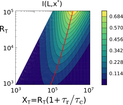
Figure S1: The mutual information $I({L};x^{\ast})$ computed via Eq. S-VII as a function of $R_{\rm T}$ and $X_{\rm T}$ for the optimal system that obeys the optimal resource allocation principle Eq. 31 of the main text: $R_{\rm T}(1+{\tau_{\rm r}}^{\ast}/{\tau_{\rm c}})=X_{\rm T}=\beta\dot{w}{\tau_{\rm r}}^{\ast}$. It is seen that for a given $X_{\rm T}$, the mutual information is maximized for $R_{\rm T}=X_{\rm T}$. This corresponds to ${\tau_{\rm r}}^{\ast}=0$, which minimizes the dynamical error: the system has given up on time integration. However, in this limit, the power diverges. In fact, an equilibrium sensing system would be superior, because it can reach, for the same number of receptors, the same sensing precision as a non-equilibrium one that does not time integrate, without turning over costly fuel Govern2014b . The observation that the membrane is very crowded suggests that the number of receptors is limiting. This leads to the design principle of Eq. 32 of the main text: $R_{\rm T}(1+{\tau_{\rm r}}^{\rm opt}/{\tau_{\rm c}})=X_{\rm T}^{\rm opt}=\beta\dot{w}^{\rm opt}{\tau_{\rm r}}^{\rm opt}$; here, the optimal integration time ${\tau_{\rm r}}^{\rm opt}$ is computed for a given $R_{\rm T}$ assuming $R_{\rm T}$ is limiting (Eq. 24 main text), while the optimal number of readout molecules $X_{\rm T}^{\rm opt}$ and the optimal power $\dot{w}^{\rm opt}$ are then set by this equation. This optimizes the design of the network for a given number of receptors $R_{\rm T}$: $X_{\rm T}^{\rm opt}$ and $\dot{w}^{\rm opt}$ are adjusted to $R_{\rm T}$ such that they are neither in excess nor limiting. Indeed, the contour plot above shows that for a given $R_{\rm T}$ there is an optimal $X_{\rm T}$, indicated by the red line; this value of $X_{\rm T}$ is close to that given by $X_{\rm T}^{\rm opt}=R_{\rm T}(1+{\tau_{\rm r}}^{\rm opt}/{\tau_{\rm c}})$ because ${\tau_{\rm r}}^{\rm opt}$, which is computed assuming $X_{\rm T}$ is in excess ($X_{\rm T}\to\infty$), is close to the optimal ${\tau_{\rm r}}$ that is computed assuming $X_{\rm T}\approx R_{\rm T}(1+{\tau_{\rm r}}/{\tau_{\rm c}})$ (the resources limit sensing like weak links in a chain, see also Fig. 3(a)). Parameters: ${\tau_{\rm c}}/{\tau_{\rm L}}=10^{-2}$; $\sigma_{L}/\overline{L}_{T}=10^{-2}$; $p$ optimized; $q^{\rm opt}$ given by $q(\Delta\mu)=4k_{\rm B}T/\Delta\mu$ such that $X_{\rm T}=\beta\dot{w}{\tau_{\rm r}}^{\ast}$.

Fig. S1 shows the mutual information $I({L};x^{\ast})$ computed via Eq. S-VII as a function of $R_{\rm T}$ and $X_{\rm T}$, with ${\tau_{\rm r}}^{\ast}$ specified via $X_{\rm T}=R_{\rm T}(1+{\tau_{\rm r}}^{\ast}/{\tau_{\rm c}})$. It is seen that for a given $X_{\rm T}$ the mutual information is maximized for $R_{\rm T}=X_{\rm T}$. This corresponds to ${\tau_{\rm r}}^{\ast}=0$: the system has become an instantaneous responder and has given up on time integration. In this limit the power diverges. In fact, an equilibrium sensing precision would be superior, because it can reach the same precision but does not need to burn fuel Govern2014b . The observation that the membrane is highly packed suggests that sensing systems employ time integration because $R_{\rm T}$ is limiting. This leads to the design principle of Eq. 32 of the main text, $R_{\rm T}(1+{\tau_{\rm r}}^{\rm opt}/{\tau_{\rm c}})=X_{\rm T}^{\rm opt}=\beta\dot{w}^{\rm opt}{\tau_{\rm r}}^{\rm opt}$, where ${\tau_{\rm r}}^{\rm opt}$ is computed in the $R_{\rm T}$-limiting regime (i.e. via Eq. 24 main text). This design principle maximizes the sensing precision for a given $R_{\rm T}$, and minimizes the number of readout molecules $X_{\rm T}$ and the power $\dot{w}$ needed to reach that precision.

Appendix S-A: The variances and co-variances

In the Fourier space we obtain as solutions of Eqs. S6 and S7

$$\delta\tilde{RL}(\omega) ={\tilde{\eta}_{RL}\over\mu+i\omega}+{\rho\delta\tilde{{L}}(\omega)\over\mu+i\omega}$$ (S86)

$$\delta\tilde{x^{*}}(\omega) ={\tilde{\eta}_{x^{*}}\over\mu^{\prime}+i\omega}+{\rho^{\prime}\delta\tilde{RL}(\omega)\over\mu^{\prime}+i\omega}.$$ (S87)

The corresponding power spectra $S_{y}(\omega)=(1/2T)\langle\delta\tilde{y}(\omega)\delta\tilde{y}(-\omega)\rangle$ of $y={L},RL,x^{*}$ are then given by the spectral addition rule Warren2006 ; Tanase-Nicola2006

$$S_{{L}}(\omega) ={2\lambda\sigma^{2}_{{L}}\over\lambda^{2}+\omega^{2}}$$ (S88)

$$S_{RL}(\omega) ={\langle\eta^{2}_{RL}\rangle\over\mu^{2}+\omega^{2}}+{\rho^{2}S_{\delta{L}}(\omega)\over\mu^{2}+\omega^{2}}$$ (S89)

$$S_{x^{*}}(\omega) ={\langle\eta^{2}_{x^{*}}\rangle\over\mu^{\prime^{2}}+\omega^{2}}+{\rho^{\prime^{2}}S_{\delta RL}(\omega)\over\mu^{\prime^{2}}+\omega^{2}},$$ (S90)

while the cross power spectra $S_{yz}(\omega)=1/(2T)\langle\delta\tilde{y}(\omega)\delta\tilde{z}(-\omega)\rangle$ are

$$S_{{L},RL}(\omega) =\frac{2k\rho}{(\lambda^{2}+\omega^{2})(\mu-i\omega)}$$ (S91)

$$S_{{L},x^{*}}(\omega) =\frac{2k\rho\rho^{\prime}}{(\lambda^{2}+\omega^{2})(\mu-i\omega)(\mu^{\prime}-i\omega)}$$ (S92)

$$S_{RL,x^{*}}(\omega) =\frac{\rho^{\prime}\langle\eta^{2}_{RL}\rangle}{(\mu^{2}+\omega^{2})(\mu^{\prime}-i\omega)}$$

$$+\frac{2k\rho^{2}\rho^{\prime}}{(\mu^{2}+\omega^{2})(\lambda^{2}+\omega^{2})(\mu^{\prime}-i\omega)}.$$ (S93)

We can now compute the noise strengths by integration, $\sigma^{2}_{yz}=1/(2\pi)\int_{-\infty}^{\infty}d\omega S_{yz}(\omega)$, resulting in the correlation matrix

$$\Sigma=\left(\begin{array}[]{ccc}\sigma^{2}_{{L}}&\sigma^{2}_{{L},RL}&\sigma^{2}_{{L},x^{*}}\\ \sigma^{2}_{{L},RL}&\sigma^{2}_{RL}&\sigma^{2}_{RL,x^{*}}\\ \sigma^{2}_{{L},x^{*}}&\sigma^{2}_{RL,x^{*}}&\sigma^{2}_{x^{*}}\end{array}\right)$$

with matrix elements

$$\sigma^{2}_{x^{*}} =f(1-f)X_{\rm T}+\frac{\rho^{\prime^{2}}}{\mu^{\prime}(\mu+\mu^{\prime})}\Big{[}p(1-p)R_{\rm T}$$

$$+\frac{\rho^{2}\sigma^{2}_{L}(\lambda+\mu+\mu^{\prime})}{\mu(\lambda+\mu)(\lambda+\mu^{\prime})}\Big{]},$$ (S94)

$$\sigma^{2}_{RL} =p(1-p)R_{\rm T}+{\rho^{2}\sigma^{2}_{L}\over\mu(\mu+\lambda)},$$ (S95)

$$\sigma^{2}_{{L},RL} ={\rho\sigma^{2}_{L}\over(\mu+\lambda)},$$ (S96)

$$\sigma^{2}_{{L},x^{*}} ={\rho\rho^{\prime}\sigma^{2}_{L}\over(\lambda+\mu)(\lambda+\mu^{\prime})},$$ (S97)

$$\sigma^{2}_{RL,x^{*}} =\frac{\rho^{\prime}}{\mu^{\prime}+\mu}\Big{[}p(1-p)R_{\rm T}+{\rho^{2}\sigma^{2}_{L}(\mu^{\prime}+\lambda+\mu)\over\mu(\lambda+\mu)(\lambda+\mu^{\prime})}\Big{]}.$$ (S98)

Appendix S-B: Variance in average receptor occupancy for fixed number of samples

Eq. S50 gives the variance in the average receptor occupancy for a fixed number of samples. To derive it, we note that

$${\rm var}\left(\frac{\sum_{i=1}^{N}n_{i}(t_{i})}{N}\middle|N\right)_{\delta{L}(t)}$$ (S99)

$$=\frac{\overline{E\langle(\sum_{i=1}^{N}n_{i}(t_{i}))^{2}\rangle}_{\delta{L}(t)}-\overline{E\langle\sum_{i=1}^{N}n_{i}(t_{i})\rangle^{2}}_{\delta{L}(t)}}{N^{2}}$$ (S100)

$$=\frac{\overline{E\langle(\sum_{i=1}^{N}n_{i}(t_{i}))^{2}\rangle_{\delta{L}(t)}}-N^{2}\overline{(p+\tilde{g}\delta{L}(t))^{2}}}{N^{2}}$$ (S101)

$$=\frac{N\overline{(p+\tilde{g}\delta{L}(t))}+N(N-1)\overline{E\langle n_{i}(t_{i})n_{j}(t_{j})\rangle}_{\delta{L}(t)}}{N^{2}}$$

$$-\overline{(p+\tilde{g}\delta{L}(t))^{2}}$$ (S102)

$$=\frac{N\overline{(p+\tilde{g}\delta{L}(t))}-N\overline{(p+\tilde{g}\delta{L}(t))^{2}}}{N^{2}}$$

$$+\frac{N(N-1)\overline{E\langle\tilde{\delta}n_{i}(t_{i})\tilde{\delta}n_{j}(t_{j})\rangle}_{\delta{L}(t)}}{N^{2}}$$ (S103)

$$=\frac{p(1-p)-\tilde{g}^{2}\sigma^{2}_{L}}{N}+\frac{N(N-1)\overline{E\langle\tilde{\delta}n_{i}(t_{i})\tilde{\delta}n_{j}(t_{j})\rangle}_{\delta{L}(t)}}{N^{2}}$$ (S104)

Here $\tilde{\delta}n_{i}(t_{i})\equiv n_{i}(t_{i})-(p+\langle n_{i}(t_{i})\rangle_{\delta{L}(t)}$ is the deviation away from the average receptor occupancy $p+\langle n_{i}(t_{i})\rangle_{\delta{L}(t)}$ when the ligand concentration at time $t$ is $\delta{L}(t)$. Here, $E$ denotes an average over the sampling times of the receptor. The average of $n_{i}(t_{i})$ over the sampling times $t_{i}$ given $\delta{L}(t)$, is $E[\langle n_{i}(t_{i})\rangle_{\delta{L}(t)}]=p+\tilde{g}\delta{L}(t)$ (see Eqs. S34 and S37). In addition, $\sigma^{2}_{L}=\langle\delta{L}(t)^{2}\rangle$ is the variance of the ligand concentration, and in going from Eq. S101 to Eq. S102 we have exploited that $n^{2}=n$. The quantity $\overline{E\langle\tilde{\delta}n_{i}(t_{i})\tilde{\delta}n_{j}(t_{j})\rangle}_{\delta{L}(t)}$ is the co-variance of the receptor occupancy given that the ligand concentration at time $t$ is $\delta{L}(t)$, and then averaged over all values of $\delta{L}(t)$, as indicated by the overline. This quantity has a contribution from the receptor switching noise and the dynamical error resulting from the ligand fluctuations.

While $\overline{E\langle\tilde{\delta}n_{i}(t_{i})\tilde{\delta}n_{j}(t_{j})\rangle}_{\delta{L}(t)}=\overline{E\langle n_{i}(t)n_{j}(t_{j})\rangle_{\delta{L}(t)}}-\overline{E\langle n_{i}\rangle_{\delta{L}(t)}\langle n_{j}\rangle_{\delta{L}(t)}}$ is the quantity that we need to compute, it is difficult to compute straightforwardly. We can however exploit the following trick Bowsher2013 . Denoting $x=n_{i}(t_{i})$, $y=n_{j}(t_{j})$ and $z=\delta{L}(t)$, we can write the quantity of interest as $\overline{E\langle\tilde{\delta}n_{i}(t_{i})\tilde{\delta}n_{j}(t_{j})\rangle}_{\delta{L}(t)}=\overline{E\langle xy\rangle_{z}}-\overline{E\langle x\rangle_{z}E\langle y\rangle_{z}}$. We can then exploit the following relation

$$\overline{E\langle\delta x\delta y\rangle}_{z} =\overline{E\langle xy\rangle}_{z}-\overline{E\langle x\rangle_{z}E\langle y\rangle_{z}}$$

$$+\overline{E\langle x\rangle_{z}E\langle y\rangle_{z}}-\overline{E\langle x\rangle_{z}}\,\,\overline{E\langle y\rangle_{z}},$$ (S105)

$$=\overline{E\langle xy\rangle}_{z}-\overline{E\langle x\rangle_{z}E\langle y\rangle_{z}}+\tilde{g}^{2}\sigma^{2}_{L}$$ (S106)

Importantly, $\overline{E\langle\delta x\delta y\rangle}_{z}$ is the co-variance related to the deviation of the receptor occupancy from the mean $p$, which is easier to compute that the deviation from $p+\tilde{g}\delta{L}(t)$. Inserting the above result into Eq. S104 yields

$${\rm var}\left(\frac{\sum_{i=1}^{N}n_{i}(t_{i})}{N}\right)_{\delta{L}(t)}$$

$$=\frac{p(1-p)}{N}+\overline{E\langle\delta n_{i}(t_{i})\delta n_{j}(t_{j})\rangle}_{\delta{L}(t)}-\tilde{g}^{2}\sigma^{2}_{L}$$ (S107)

where we have used that $N(N-1)\approx N^{2}$ for $N\gg 1$.

Appendix S-C: The reliability factor $q$

Here we derive the expression for the reliability factor $q$ in terms of the fundamental rate constants, $k_{\rm f}$, $k_{\rm-f}$, $k_{\rm r}$, $k_{\rm-r}$, which is used to derive the principal result of the main text, Eq. 20 (i.e. Eq. S81 above). We first note that

$$e^{\beta\Delta\mu_{1}}-1 =\frac{k_{\rm f}\overline{x}}{k_{\rm-f}\overline{x^{*}}}-1$$

$$=\frac{k_{\rm f}(k_{\rm r}+k_{\rm-f}pR_{T})}{k_{\rm-f}(k_{-\rm r}+k_{\rm f}pR_{T})}-1=\frac{k_{\rm f}k_{\rm r}-k_{\rm-f}k_{\rm-r}}{k_{\rm-f}(k_{\rm-r}+k_{\rm f}pR_{T})}.$$ (S108)

$$e^{\beta\Delta\mu_{2}}-1 =\frac{k_{\rm r}\overline{x^{*}}}{k_{\rm-r}\overline{x}}-1$$

$$=\frac{k_{\rm r}(k_{\rm-r}+k_{\rm f}pR_{T})}{k_{\rm-r}(k_{\rm r}+k_{\rm-f}pR_{T})}-1=\frac{(k_{\rm f}k_{\rm r}-k_{\rm-f}k_{\rm-r})pR_{T}}{k_{\rm-r}(k_{\rm r}+k_{\rm-f}pR_{T})}.$$ (S109)

Noting that $\Delta\mu=\Delta\mu_{1}+\Delta\mu_{2}$, we find that

$$e^{\beta\Delta\mu}-1 =\frac{k_{\rm f}k_{\rm r}}{k_{\rm-f}k_{\rm-r}}-1=\frac{k_{\rm f}k_{\rm r}-k_{\rm-f}k_{\rm-r}}{k_{\rm-f}k_{\rm-r}}.$$ (S110)

Combining the above results yields the reliability factor $q$:

$$q \equiv\frac{(e^{\beta\Delta\mu_{1}}-1)(e^{\beta\Delta\mu_{2}}-1)}{e^{\beta\Delta\mu}-1}$$

$$=\frac{(k_{\rm f}k_{\rm r}-k_{\rm-f}k_{\rm-r})pR_{T}}{(k_{\rm-r}+k_{\rm f}pR_{T})(k_{\rm r}+k_{\rm-f}pR_{T})}$$ (S111)

In order to obtain an expression for the reliability factor $q$ that does not explicitly depend on the rate constants, we notice that the flux of readout activation $\dot{n}$ can be expressed as

$$\dot{n} \equiv k_{\rm f}\overline{RL}\overline{x}-k_{\rm-f}\overline{RL}\overline{x^{*}}$$

$$=k_{\rm f}pR_{\rm T}(1-f)X_{\rm T}-k_{\rm-f}pR_{\rm T}fX_{\rm T}$$

$$=pR_{\rm T}X_{\rm T}[k_{\rm f}(1-f)-k_{\rm-f}f]$$

$$=pR_{\rm T}X_{\rm T}[k_{\rm f}(k_{\rm-f}pR_{\rm T}+k_{\rm r}){\tau_{\rm r}}-k_{\rm-f}(k_{\rm f}pR_{\rm T}+k_{\rm-r}){\tau_{\rm r}}]$$

$$=pR_{\rm T}X_{\rm T}{\tau_{\rm r}}(k_{\rm f}k_{\rm r}-k_{\rm-f}k_{\rm-r}),$$ (S112)

where in the forth line we have exploited that $f=(k_{\rm f}pR_{\rm T}+k_{\rm-r}){\tau_{\rm r}}$. Substituting $(k_{\rm f}k_{\rm r}-k_{\rm-f}k_{\rm-r})pR_{\rm T}=\dot{n}/(X_{\rm T}{\tau_{\rm r}})$ into Eq. S111 and exploiting again the expression for $f$ yields for the reliability factor $q$

$$q =\frac{\dot{n}{\tau_{\rm r}}}{f(1-f)X_{T}}.$$ (S113)

This expression shows that the flux $\dot{n}$ can also be expressed as a function of $q$, namely

$$\dot{n} =f(1-f)X_{\rm T}q/{\tau_{\rm r}}.$$ (S114)

Finally, the reliability factor $q$ can also be expressed in terms of the variable $\rho^{\prime}=k_{\rm f}(1-f)X_{\rm T}-k_{\rm-f}fX_{\rm T}$ by rewriting the flux $\dot{n}$ as

$$\dot{n} =pR_{\rm T}X_{\rm T}[k_{\rm f}(1-f)-k_{\rm-f}f]=\rho^{\prime}pR_{\rm T},$$ (S115)

yielding for $q$

$$q =\frac{\rho^{\prime}pR_{\rm T}{\tau_{\rm r}}}{f(1-f)X_{T}}.$$ (S116)

References

- [1] H.C. Berg and E.M. Purcell. Physics of chemoreception. Biophys. J., 20(2):193–219, November 1977.
- [2] V. Sourjik and H.C. Berg. Receptor sensitivity in bacterial chemotaxis. Proc. Natl. Acad. Sci. USA, 99(1):123–127, 2002.
- [3] M. Ueda and T. Shibata. Stochastic signal processing and transduction in chemotactic response of eukaryotic cells. Biophys. J., 93(1):11–20, 2007.
- [4] W. Bialek and S. Setayeshgar. Physical limits to biochemical signaling. Proc. Natl. Acad. Sci. USA, 102(29):10040–10045, 2005.
- [5] K. Wang, W.J. Rappel, R. Kerr, and H. Levine. Quantifying noise levels of intercellular signals. Phys. Rev. E, 75(6):061905, 2007.
- [6] W.J. Rappel and H. Levine. Receptor noise and directional sensing in eukaryotic chemotaxis. Phys. Rev. Lett., 100(22):228101, 2008.
- [7] R.G. Endres and N.S. Wingreen. Maximum likelihood and the single receptor. Phys. Rev. Lett., 103(15):158101, 2009.
- [8] B. Hu, W. Chen, W.J. Rappel, and H. Levine. Physical limits on cellular sensing of spatial gradients. Phys. Rev. Lett., 105(4):048104, 2010.
- [9] T. Mora and N.S. Wingreen. Limits of sensing temporal concentration changes by single cells. Phys. Rev. Lett., 104(24):248101, 2010.
- [10] P. Mehta and D.J. Schwab. Energetic Costs of Cellular Computation. Proc. Natl. Acad. Sci. USA, 109(44):17978, 2012.
- [11] C.C. Govern and P.R. ten Wolde. Fundamental limits on sensing chemical concentrations with linear biochemical networks. Phys. Rev. Lett., 109:218103, 2012.
- [12] C.C. Govern and P.R. ten Wolde. Optimal resource allocation in cellular sensing systems. Proc. Natl. Acad. Sci. USA, 111(49):17486–17491, 2014.
- [13] C.C. Govern and P.R. ten Wolde. Energy Dissipation and Noise Correlations in Biochemical Sensing. Phys. Rev. Lett., 113:258102, 2014.
- [14] K. Kaizu, W. De Ronde, J. Paijmans, K. Takahashi, F. Tostevin, and P.R. ten Wolde. The Berg-Purcell limit revisited. Biophysical Journal, 106(4):976–985, 2014.
- [15] A. Mugler, A. Levchenko, and I. Nemenman. Limits to the precision of gradient sensing with spatial communication and temporal integration. Proc. Natl. Acad. Sci. USA, 113(6):E689–E695, February 2016.
- [16] S. Fancher and A. Mugler. Fundamental limits to collective concentration sensing in cell populations. Phys. Rev. Lett., 118(7):078101, February 2017.
- [17] P.R. ten Wolde, N.B. Becker, T.E. Ouldridge, and A. Mugler. Fundamental limits to cellular sensing. J. Stat. Phys., 162(5):1395–1424, January 2016.
- [18] N.B. Becker, A. Mugler, and P.R. ten Wolde. Optimal prediction by cellular signaling networks. Phys. Rev. Lett., 115:258103, 2015.
- [19] L. Durrieu, D. Kirrmaier, T. Schneidt, I. Kats, S. Raghavan, L. Hufnagel, T.E. Saunders, and M. Knop. Bicoid gradient formation mechanism and dynamics revealed by protein lifetime analysis. Mol. Syst. Biol., 14(9):e8355–15, 2018.
- [20] F. Tostevin and P.R. ten Wolde. Mutual information between input and output trajectories of biochemical networks. Phys. Rev. Lett., 102:218101, 2009.
- [21] P. Sartori and Y. Tu. Noise filtering strategies in adaptive biochemical signaling networks. J. Stat. Phys., 142(6):1206–1217, 2011.
- [22] J. Long, S.W. Zucker, and T. Emonet. Feedback between motion and sensation provides nonlinear boost in run-and-tumble navigation. PLoS Comput. Biol., 13(3):e1005429, 2017.
- [23] M. Monti, D.K. Lubensky, and P.R. ten Wolde. Robustness of clocks to input noise. Phys. Rev. Lett., 121(7):078101, 2018.
- [24] A Goldbeter and D E Koshland. An amplified sensitivity arising from covalent modification in biological systems. Proc. Natl. Acad. Sci. U. S. A., 78(11):6840–6844, 1981.
- [25] U. Alon. Introduction to Systems Biology: Design Principles of Biological Networks. CRC press, Boca Raton, FL, 2007.
- [26] A.H. Lang, C.K. Fisher, T. Mora, and P. Mehta. Thermodynamics of statistical inference by cells. Phys. Rev. Lett., 113(14):148103, 2014.
- [27] D. Hartich and U. Seifert. Optimal inference strategies and their implications for the linear noise approximation. Phys. Rev. E, 94(4):042416–11, 2016.
- [28] F. Tostevin and P.R. ten Wolde. Mutual information in time-varying biochemical systems. Phys. Rev. E, 81:061917, 2010.
- [29] A. Hilfinger and J. Paulsson. Separating intrinsic from extrinsic fluctuations in dynamic biological systems. Proc. Natl. Acad. Sci. USA, 108(29):12167–12172, 2011.
- [30] C.G. Bowsher, M. Voliotis, and P.S. Swain. The fidelity of dynamic signaling by noisy biomolecular networks. PLoS Comput. Biol., 9(3), 2013.
- [31] Because the system is stationary and time-invariant, we can omit the argument in and write .
- [32] T.E. Ouldridge, C.C. Govern, and P.R. ten Wolde. Thermodynamics of computational copying in biochemical systems. Phys. Rev. X, 7(2):021004, 2017.
- [33] M. Li and G.L. Hazelbauer. Cellular stoichiometry of the components of the chemotaxis signaling complex. J. Bacteriol., 186(12):3687–3694, 2004.
- [34] A. Vaknin and H.C. Berg. Physical responses of bacterial chemoreceptors. J. Mol. Biol., 366(5):1416–1423, 2007.
- [35] M.A. Danielson, H.P. Biemann, D.E. Koshland, Jr. Falke, and J.J. Falke. Attractant- and disulfide-induced conformational changes in the ligand binding domain of the chemotaxis aspartate receptor: a 19F NMR study. Biochemistry, 33(20):6100–6109, 1994.
- [36] H.C. Berg and D.A. Brown. Chemotaxis in Escherichia coli analysed by three-dimensional tracking. Nature, 239(5374):500–504, 1972.
- [37] K.M. Taute, S. Gude, S.J. Tans, and T.S. Shimizu. High-throughput 3D tracking of bacteria on a standard phase contrast microscope. Nat. Commun., 6:1–9, 2015.
- [38] L. Jiang, Q. Ouyang, and Y. Tu. Quantitative modeling of Escherichia coli chemotactic motion in environments varying in space and time. PLoS Comput. Biol., 6(4):e1000735–12, 2010.
- [39] M. Flores, T.S. Shimizu, P.R. ten Wolde, and F. Tostevin. Signaling noise enhances chemotactic drift of E. coli. Phys. Rev. Lett., 109(14):148101, 2012.
- [40] T.S. Shimizu, Y. Tu, and H.C. Berg. A modular gradient-sensing network for chemotaxis in Escherichia coli revealed by responses to time-varying stimuli. Mol. Syst. Biol., 6:1–14, 2010.
- [41] V. Sourjik and H.C. Berg. Binding of the Escherichia coli response regulator CheY to its target measured in vivo by fluorescence resonance energy transfer. Proc. Natl. Acad. Sci. USA, 99(20):12669–12674, 2002.
- [42] Monica Skoge, Yigal Meir, and Ned S Wingreen. Dynamics of cooperativity in chemical sensing among cell-surface receptors. Phys. Rev. Lett., 107:178101, 2011.
- [43] A.C. Barato, D. Hartich, and U. Seifert. Efficiency of cellular information processing. New J. Phys., 16:103024, 2014.
- [44] J.M. Horowitz and M. Esposito. Thermodynamics with continuous information flow. Phys. Rev. X, 4:031015, 2014.
- [45] D. Hartich, A.C. Barato, and U. Seifert. Sensory capacity: An information theoretical measure of the performance of a sensor. Phys. Rev. E, 93(2):022116–14, 2016.
- [46] R.A. Brittain, N.S. Jones, and T.E. Ouldridge. What we learn from the learning rate. J. Stat. Mech., 2017(6):063502–22, 2017.
- [47] G. Lan, P. Sartori, S. Neumann, V. Sourjik, and Y. Tu. The energy–speed–accuracy trade-off in sensory adaptation. Nat. Phys., 8(5):422–428, 2012.
- [48] P. Sartori and Y. Tu. Free energy cost of reducing noise while maintaining a high sensitivity. Phys. Rev. Lett., 115(11):118102, 2015.
- [49] D.T. Gillespie. The chemical Langevin equation. J. Chem. Phys., 113(1):297–306, 2000.
- [50] C.W. Gardiner. Stochastic methods. Springer-Verlag, Berlin–Heidelberg–New York–Tokyo, 2009.
- [51] P.B. Warren, S. Tânase-Nicola, and P.R. ten Wolde. Exact results for noise power spectra in linear biochemical reaction networks. J. Chem. Phys., 125(14):144904, 2006.
- [52] S. Tanase-Nicola, P.B. Warren, and P.R. ten Wolde. Signal detection, modularity, and the correlation between extrinsic and intrinsic noise in biochemical networks. Phys. Rev. Lett., 97:068102, 2006.
- [53] A.M. Walczak, A. Mugler, and C.H. Wiggins. Analytic methods for modeling stochastic regulatory networks. Computational Modeling of Signaling Networks, 880:273–322, 2012.
- [54] N. G. Van Kampen. Stochastic processes in physics and chemistry. North Holland, Amsterdam, 1992.
- [55] E. Ziv, I. Nemenman, and C.H. Wiggins. Optimal signal processing in small stochastic biochemical networks. PLoS ONE, 2(10):e1077, 2007.
- [56] C. Shannon. Bell Syst. Tech. J., 27:623, 1948.
- [57] S.G. Das, M. Rao, and G. Iyengar. Universal lower bound on the free-energy cost of molecular measurements. Phys. Rev. E, 95(6):062410, 2017.