Explosive, oscillatory and Leidenfrost boiling at the nanoscale

Summarium

We investigate the different boiling regimes around a single continuously laser-heated $80\text{\,}\mathrm{nm}$ gold nanoparticle and draw parallels to the classical picture of boiling. Initially, nanoscale boiling takes the form of transient, inertia-driven, unsustainable boiling events characteristic of a nanoscale boiling crisis. At higher heating power, nanoscale boiling is continuous, with a vapor film being sustained during heating for at least up to $20\text{\,}\mathrm{\SIUnitSymbolMicro s}$. Only at high heating powers does a substantial stable vapor nanobubble form. At intermediate heating powers, unstable boiling sometimes takes the form of remarkably stable nanobubble oscillations with frequencies between $40\text{\,}\mathrm{MHz}60\text{\,}\mathrm{MHz}$; frequencies that are consistent with the relevant size scales according to the Rayleigh-Plesset model of bubble oscillation, though how applicable that model is to plasmonic vapor nanobubbles is not clear.

I Introduction

The mechanisms involved in boiling of liquids in contact with a heat source are of crucial importance when it comes to understanding and optimizing heat transfer, particularly in applications requiring the removal of high heat flux. In recent years, there has been particular interest in the effect that the use of ‘nanofluids’—fluids containing metal nanoparticles that may attach to device walls Murshed et al. (2011); Taylor and Phelan (2009)—and nanostructured surfaces have on pool-boiling heat transfer into the fluid Kim et al. (2015). There are many reports of both nanofluids and nanoscale surface roughness increasing the critical heat flux that a heating device can support. It is therefore imperative to gain a deeper understanding of boiling at the nanoscale, a topic we hope to shed some light on here.

In the canonical model of pool boiling, i.e., boiling of a large ‘pool’ of liquid through direct contact with a hot surface, boiling is thought to occur in three primary regimes: in order of increasing relative temperature $\Delta T$, nucleate boiling, transition boiling, and film boiling (see Fig. 1).

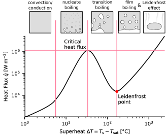
Descriptio 1: The well-known traditional boiling curve of macroscopic pools of water at atmospheric pressure with sketches of the different boiling regimes. Curve data adapted from Ref. Çengel (2003).

In nucleate boiling, boiling occurs at a myriad microscopic active vapor generating centers from which small bubbles rise upward (gravity is significant for common liquids at human size scales), and the resulting total heat flux from the heating surface to the liquid being boiled is proportional to the number of active vapor generating centers (bubble nucleation sites) at any given time. It is well-established that, apart from depending on $\Delta T$, this number depends on the structure of the heater surface—broadly speaking, rougher surfaces support more vapor nucleation sites—but how a particular surface geometry will lead to particular boiling characteristics is not currently understood Pioro et al. (2004a); *pioro_nucleate_2004-1; Dong et al. (2014).

As the temperature and heat flux increase, an ever greater proportion of the surface will be covered by vapor bubbles. The vapor, with its much lower thermal conductivity as compared to the corresponding liquid, acts as a thermal insulator. This leads to the heat flux topping out at a critical heat flux and then falling as the temperature and the vapor coverage of the heater increase. This phenomenon is known as the boiling crisis. The boiling behavior as the heat flux falls is characterized by large vapor bubbles forming at the heating surface and rising violently, and is referred to as transition boiling or unstable film boiling Kim et al. (2015); Jakob and Linke (1933, 1935); Çengel (2003).

If the temperatures are high enough to overcome the thermally insulating effect of a thin vapor film, boiling can stabilize into so-called film boiling. In the case of small drops of water coming into contact with a larger heating surface, this leads to drops levitating on a cushion of hot vapor. The heat flux again increases with temperature; the point of minimum heat flux is known as the Leidenfrost point, and the transition into film boiling is popularly known as the Leidenfrost effect—both named after Johann Gottlob Leidenfrost, who described the effect in 1756 Leidenfrost (1756); *[Translation:][]leidenfrost_fixation_1966.

While the precise thresholds and dynamics depend on various properties of the heater, from the material’s thermal properties and surface microstructure up to the macroscopic shape Sher et al. (2012), the broad outline of the behavior as described above is widely applicable.

In this work, we dive down to the nanoscale using the tools provided by modern optical microscopy and study submicrosecond boiling dynamics at a single artificial nucleation site in the form of a laser-heated gold nanoparticle (AuNP); AuNPs are frequently used to optically generate vapor micro- and nanobubbles Hou et al. (2015); Baffou et al. (2014); Siems et al. (2011); Boulais et al. (2012); Hashimoto et al. (2012); Lombard et al. (2014, 2015); Setoura et al. (2017); Li et al. (2017). We will find striking parallels to the progression of a macroscopic system through the boiling crisis, in which the entire heater surface dries out when a thermally insulating vapor film forms, and the heat flux plummets.

II Method

This work follows on from our previously published results Hou et al. (2015), in which we described an unstable, explosive nanoscale boiling regime arising under continuous heating, near the threshold heating power for boiling. Using mostly the same technique, here we investigate in detail the various dynamics arising from a much broader range of different heating powers, with an emphasis on exploring the parameter space beyond the threshold.

Gold nanospheres with a diameter of $80\text{\,}\mathrm{nm}$ (from NanoPartz) are immobilized on a cover glass at very low surface coverage by spin-coating. The nanoparticles are submerged in a large reservoir of n-pentane and investigated optically in a photothermal–confocal microscope described in previous work Hou et al. (2015); Gaiduk et al. (2010): two continuous-wave laser beams, a heating beam and a probe beam, are carefully overlapped and tightly focused on the same nanoparticle. The heating beam is partly absorbed by the sample; the deposited energy and associated temperature increase lead to localized changes in the sample, e.g., in density. These changes affect how much the probe beam is scattered.

In photothermal microscopy, these small heating-induced changes can be used to measure a nano-object’s absorption cross section Jollans et al. (2019). In this work, we focus on the dynamics of the response, specifically in the case of boiling, instead.

n-Pentane was chosen as a medium, as in our previous work, due to its boiling point under ambient conditions (viz. ca. $36\text{\,}\mathrm{\SIUnitSymbolCelsius}$) being close to room temperature; the intention of this choice was to reduce the necessary heating powers and the impact of heating-related damage to the AuNPs.

A single gold nanoparticle—identified through photothermal contrast—is heated using a focused near-resonant [$532\text{\,}\mathrm{nm}$; cf. Fig. 2(c)] laser, the intensity of which is controlled using an acousto-optic modulator (AOM) and monitored using a fast photodiode. The nanoparticle is monitored in real time through the back-scattering of an off-resonant probe laser ($815\text{\,}\mathrm{nm}$), measured using another fast photodiode. Our real-time single-nanoparticle optical measurements allow us to noninvasively follow the dynamics of boiling and vapor nanobubble formation around the AuNP with a high time resolution, limited by the $80\text{\,}\mathrm{MHz}$ cut-off frequency ($-3\text{\,}\mathrm{dB}$) of our detector.

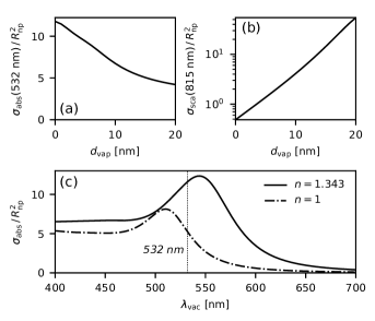
Descriptio 2: Layered-sphere Mie theory calculation Peña and Pal (2009) with an $80\text{\,}\mathrm{nm}$ diameter gold core and a vacuum shell (bubble, $n=1$) of varying thickness $d_{\mathrm{vap}}$ in a medium with refractive index $n=1.33$. (a) Absorption of $\lambda_{\mathrm{vac}}=$532\text{\,}\mathrm{nm}$$ and (b) scattering of $\lambda_{\mathrm{vac}}=$815\text{\,}\mathrm{nm}$$, both shown as a function of bubble thickness. (c) Absorption spectra of $80\text{\,}\mathrm{nm}$ AuNPs, when in $n$-pentane as compared to vacuum. See also: Appendix A.

It is important to note at this point that a given heating laser intensity uniquely determines neither the absorbed heating power nor the temperature of the AuNP. Rather, the absorption cross section $\sigma_{\mathrm{abs}}$ of the AuNP, and with it the absorbed power, depends strongly on the environment: The localized surface plasmon resonance of the AuNP depends on the refractive index of the environment, i.e., on whether the AuNP is surrounded by liquid ($n\approx 1.33$) or vapor ($n\simeq 1$).

Modeling the nanoparticle surrounded by a vapor layer as a multilayered sphere with a gold core and a shell with a refractive index of $n=1$ and with a certain thickness $d_{\mathrm{vap}}$, a layered-sphere Mie theory calculation Peña and Pal (2009) can give us an idea of how $\sigma_{\mathrm{abs}}$ changes upon nanobubble growth: Fig. 2(a) shows $\sigma_{\mathrm{abs}}$ dropping by $10\text{\,}\mathrm{\char 37\relax}$ with only a $3\text{\,}\mathrm{nm}$ thick bubble, and by half with $13\text{\,}\mathrm{nm}$ thickness. This leads to negative feedback as a vapor shell grows due to its optical properties. This complements the negative feedback due to the shell’s thermal properties which is known from the classical Leidenfrost effect.

At the same time, the dependence of our read-out, the back-scattering at $815\text{\,}\mathrm{nm}$, on the bubble size is not trivial. As Fig. 2(b) shows, for sufficiently thin vapor nanobubbles, we can expect the scattering to grow steeply with the bubble thickness.

The AuNP is initially subjected to a heating laser intensity such that it is near the boiling threshold, but below it; then, periodically, the AOM is switched to provide a pulse of some microseconds at a higher illumination intensity (duty cycle: $1\text{\,}\mathrm{\char 37\relax}$).

The baseline intensity is chosen heuristically on a nanoparticle-by-nanoparticle basis by testing increasing baselines with a fixed additional on-pulse intensity until the measured scattering shows a significant change. The chosen baseline intensity is between $80\text{\,}\mathrm{\SIUnitSymbolMicro W}$ and $140\text{\,}\mathrm{\SIUnitSymbolMicro W}$ as measured in the back focal plane. The pulse length, pulse height, and baseline can then be changed at will between timetrace acquisitions; the length of a full timetrace was $10\text{\,}\mathrm{ms}$, of which the intensity is ‘high’ for $100\text{\,}\mathrm{\SIUnitSymbolMicro s}$. Between subsequent acquisitions, a few seconds of dead time pass while data is stored and conditions are, as the case may be, changed.

III Results

III.1 Nanoscale boiling regimes

Depending on the heating power during the heating pulse, boiling around the nanoparticles was observed to follow four distinct patterns as shown in figure 3, before irreversible damage sets in at higher powers:

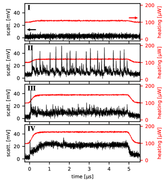
Descriptio 3: Single-shot scattering timetraces of the same $80\text{\,}\mathrm{nm}$ Au sphere. Black: scattering in the detector’s units; red: heating intensity in the back focal plane. Four principal regimes of heated AuNP behavior are observed: (I) below boiling threshold; small thermal lensing effect. (II) near boiling threshold; repeated short-lived vapor nanobubble formation. (III) above boiling threshold; unstable vapor nanobubble for the duration of heating. (IV) far above threshold; relatively stable nanobubble, probable damage to AuNP. See also: figure 4

I.—At sufficiently low power, the effect of heating the AuNP is limited to a small thermal lensing effect that cannot easily be directly identified from the timetrace as shown. There is no indication of boiling.

II.—Above a certain threshold, $\sim$120\text{\,}\mathrm{\SIUnitSymbolMicro W}$$ in the back focal plane with some variation from particle to particle, as previously demonstrated Hou et al. (2015), strong $\sim$1\text{\times}{10}^{-8}\text{\,}\mathrm{s}$$ spikes with similar peak values start appearing at random intervals. These can be explained by rapid inertially driven expansion of a vapor nanobubble around the AuNP; in the presence of this vapor shell, the hot AuNP experiences a boiling crisis and the nanobubble collapses immediately. While this behavior is reminiscent of intermittent film boiling, averaged over many disperse vapor generating centers it should appear as nucleate boiling from a distance.

III.—As the power is increased further, beyond around $150\text{\,}\mathrm{\SIUnitSymbolMicro W}$, all distinct explosive spikes but the first disappear. In their place, the initial explosion is followed by still highly dynamic behavior, notably with a much smaller amplitude. It appears that while in the previous case, the AuNP returned to the same state after the boiling events (i.e., no vapor), now, it does not; after the initial expansion, the nanobubble does not appear to fully collapse, but rather to reduce to a sustainable if not particularly stable size. We can think of this as a transition boiling regime.

IV.—At extremely high powers, the signal steadily grows [as expected for a growing vapor bubble; cf. Fig. 2(b)], after the initial spike, to a stable level that is maintained until heating ends. The signal overall appears calmer than in the previous cases. In analogy with the Leidenfrost effect known macroscopically, it appears that a nanometer-scale vapor film around the heated AuNP is stabilized only at these substantial heating powers.

Note that in the explosive regime (II), all events are clearly separated from one another, and all have approximately the same maximum value. In particular, no double-peaks have been observed. This indicates that each nanoparticle hosts only a single vapor generating center.

In sustained boiling regimes (III, IV), nanobubble behavior qualitatively stays the same from after the initial expansion until the heating intensity is reduced, for at least up to $20\text{\,}\mathrm{\SIUnitSymbolMicro s}$: long-lived vapor nanobubbles do not appear to spontaneously collapse without a change in externally imposed conditions.

However, extended or repeated irradiation at powers sufficient for boiling will cause irreversible damage to the nanoparticle: in particular, after minutes of irradiation at high power, lower powers no longer show the familiar explosive nucleate boiling events. We cannot tell in what way the particles change during long experiments. They might be melting, which could involve changing surface structure and/or contact area with the substrate, they might be fragmenting Setoura et al. (2014), or they may be sinking into the substrate Hashimoto et al. (2009). Any one of these possibilities would change the optical and thermal properties in hard-to-predict ways.

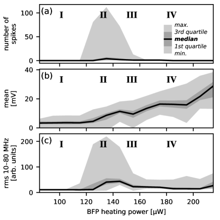
Descriptio 4: Dependence of vapor nanobubble behavior on laser power, based on 8050 single-shot time traces measured at one nanoparticle, like those shown in figure 3. (a) number of spikes (extrema $\mathrm{d}\tilde{u}\big{/}\mathrm{d}t=0$ where $\mathrm{d}^{2}\tilde{u}\big{/}\mathrm{d}t^{2}<0$ is below a heuristically chosen threshold, $\tilde{u}(t)$ being the signal smoothed with a $30\text{\,}\mathrm{ns}$ Hann filter) in the signal. (b) mean scattering signal during heating. (c) RMS power of the frequency components between $10\text{\,}\mathrm{MHz}80\text{\,}\mathrm{MHz}$.

Figure 4 shows how the behavior varies with heating power; in particular, the explosive regime (II) clearly occurs only in a limited temperature range. Note also that the mean response does not have an equivalent to the nucleate boiling peak in the classical curve from figure 1.

III.2 Stable vapor nanobubble oscillations

For some nanoparticles, heating powers characterized by unstable boiling were found to produce not a randomly growing and collapsing vapor nanobubble, but a stable and surprisingly pure oscillation with frequencies around $50\pm 10\text{\,}\mathrm{MHz}$ (see Fig. 5).

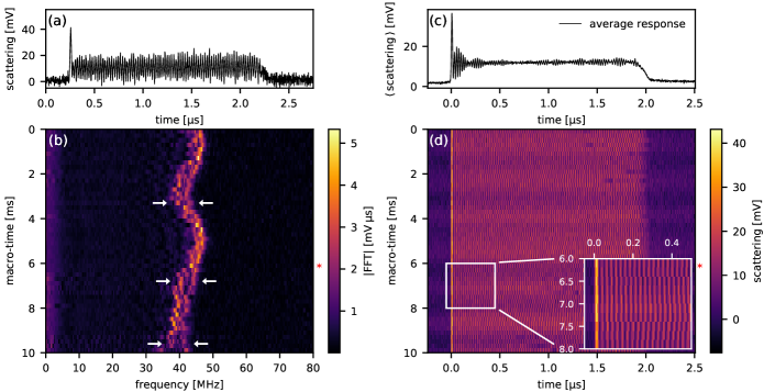
Descriptio 5: Nanobubble oscillations; (a) Single-shot nanobubble timetrace with clearly visible oscillations. (b) Fourier transforms of 50 subsequent such timetraces of the same AuNP subject to an unchanging heating profile. White arrows highlight some points with particularly clear frequency splitting. (c) Average of the timetraces in panel (d), synchronized on the initial rising edge. (d) Fifty timetraces used in panels (b) and (c). In panels (b) and (d), the lines marked with an asterisk correspond to panel (a).

To crudely model the oscillations, we shall employ the Rayleigh-Plesset model Lauterborn and Kurz (2010) for spherical gas bubble oscillations, which has been shown theoretically to be remarkably effective for describing the kinetics of the initial expansion and collapse of a plasmonic vapor nanobubble Lombard et al. (2014, 2015):

$$\varrho R\ddot{R}+\frac{3}{2}\varrho\dot{R}^{2}\leavevmode\nobreak\ =\leavevmode\nobreak\ p_{\mathrm{g}}\left(\frac{R_{0}}{R}\right)^{3\kappa}-p_{\mathrm{a}}-\frac{\mathrm{2\gamma}}{R}-\frac{3\mu}{R}\dot{R},$$ (1)

$$\mathrm{with}\leavevmode\nobreak\ \leavevmode\nobreak\ \leavevmode\nobreak\ p_{\mathrm{g}}\leavevmode\nobreak\ =\leavevmode\nobreak\ \frac{2\gamma}{R_{0}}+p_{\mathrm{a}},$$ (2)

where $R$ is bubble radius, $R_{0}$ is the equilibrium radius, $\kappa=c_{p}/c_{V}$ is the polytropic exponent, $\gamma$ is the surface tension, $\mu$ the dynamic viscosity, $\varrho$ the liquid density, $p_{\mathrm{a}}$ the ambient (static) pressure, and $p_{\mathrm{g}}$ the gas bubble pressure at rest.

Compared to the full Rayleigh-Plesset equation as given by Lauterborn and Kurz (2010), we are assuming no external ultrasound field and make no distinction between vapor and gas pressure. The latter approximation is an adiabatic approximation—it forbids mass transfer between the bubble and the liquid at the relevant timescales. If the bubble were to be understood classically as vapor, meaning vapor molecules can freely condense into the surrounding liquid, then there would be no restorative force due to compression when the size of the bubble is reduced; there could be no oscillation. Oscillations are, however, clearly observed. Hence, we proceed assuming full conservation of mass for the material inside the bubble, i.e., we treat the vapor nanobubble as a classical gas bubble. (N.B., the applicability of the model is further discussed in Appendix B.)

Expanding eq. (1) for small perturbations $R=R_{0}(1+\varepsilon)$ from the equilibrium to first order in $\varepsilon$, we can reduce the Rayleigh-Plesset model to a damped harmonic oscillator,

$$\frac{\mathrm{d}^{2}\varepsilon}{\mathrm{d}t^{2}} +2\zeta\omega_{0}\frac{\mathrm{d}\varepsilon}{\mathrm{d}t}+\omega_{0}^{2}\varepsilon=0,$$ (3)

$$\mathrm{where}\leavevmode\nobreak\ \omega_{0}\leavevmode\nobreak\ =\leavevmode\nobreak\ \frac{1}{R_{0}\sqrt{\varrho}}\sqrt{3\kappa p_{\mathrm{a}}+\frac{2\gamma}{R_{0}}\big{(}3\kappa-1\big{)}}$$ (4)

$$\mathrm{and}\leavevmode\nobreak\ \zeta\leavevmode\nobreak\ =\leavevmode\nobreak\ \frac{3\mu}{2\varrho R_{0}^{\,2}\;\omega_{0}}.$$ (5)

This allows us to calculate the resonance frequency $f=\omega_{0}\sqrt{1-\zeta^{2}}/2\pi$, shown in Fig. 6, using the well-known material properties of pentane noa (2018) at the saturation point Vesovic at $p_{\mathrm{a}}=$1\text{\,}\mathrm{atm}$$: $f=$40\text{\,}\mathrm{MHz}$$ corresponds to $R_{0}=$142\text{\,}\mathrm{nm}$$. The influence of viscous damping has a negligible impact on the resonance frequency as $\zeta\sim 0.1$ is small; in the real system, damping seems to be counteracted by the driving force from heating, leading to stable self-oscillation.

We can take into account the temperature- and pressure-dependence of the density $\varrho(T,p_{\mathrm{g}})$ and surface tension $\gamma(T,p_{\mathrm{g}})$ by using the values for saturated liquid at $p_{\mathrm{g}}=p_{\mathrm{a}}+2\gamma/R_{0}$ and the saturation temperature $T=T_{\mathrm{sat}}(p_{\mathrm{g}})$. If we do this, the results are only slightly changed: then, $f=$40\text{\,}\mathrm{MHz}$$ corresponds to $R_{0}=$136\text{\,}\mathrm{nm}$$.

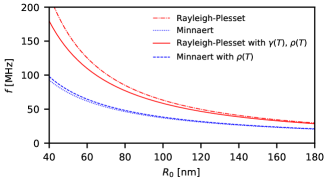
Descriptio 6: Resonance frequencies for vapor nanobubbles in pentane, according to the Rayleigh-Plesset and Minnaert models, with and without considering the temperature dependence of the surface tension $\gamma$ and the density $\varrho$.

It is interesting to note that the two terms under the square root in eq. (4), $3\kappa p_{\mathrm{a}}=$0.33\text{\,}\mathrm{MPa}$$ and $2\gamma(3\kappa-1)/$136\text{\,}\mathrm{nm}$=$0.36\text{\,}\mathrm{MPa}$$, are of the same order of magnitude. The resulting frequencies, then, are not dramatically different from those predicted by the much simpler Minnaert model. In 1933, Marcel Minnaert proposed a simple model to explain the ‘musical’, i.e., audible, oscillations of spherical air bubbles in a stream of water (e.g. from a tap) Minnaert (1933), which does not consider surface tension or viscous drag, only the compressibility of the gas:

$$\omega_{\mathrm{Minnaert}}=\frac{1}{R_{0}}\sqrt{\frac{3\kappa p_{\mathrm{a}}}{\varrho}}$$ (6)

In any case, all oscillation frequencies observed correspond to radii larger than the radius of the AuNP (viz. $R_{\mathrm{np}}=$40\text{\,}\mathrm{nm}$$), up to approximately the size of the near diffraction-limited focus of the heating laser (viz. FWHM $w_{\mathrm{\perp}}=$0.2\text{\,}\mathrm{\SIUnitSymbolMicro m}$,\leavevmode\nobreak\ w_{\mathrm{\parallel}}=$0.6\text{\,}\mathrm{\SIUnitSymbolMicro m}$$). Direct measurement of bubble size is not possible with the present technique, but these estimates are in agreement with previous measurements of vapor nanobubble sizes .

The factors contributing to the oscillations are evidently not random: as Figs. 5(b)–5(d) show, the frequencies are strongly correlated from one event to the next; the resonance frequency appears to drift back and forth over time at audio frequencies, perhaps as a response to acoustic noise or small vibrations in the microscope. As the other examples in Fig. 7 demonstrate, both the rate and periodicity of the frequency drift vary from measurement to measurement.

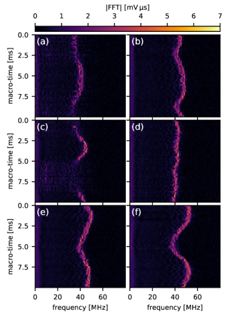
Descriptio 7: Example series of oscillating-bubble event Fourier transforms, all for the same nanoparticle, in the same form as Fig. 5(b).

Additionally, as shown in figure 8, oscillation frequencies vary from particle to particle, as well as from moment to moment under constant experimental conditions. For some, but not all, nanoparticles, the mean oscillation frequency appears to increase with heating power. However, as all the measurements were taken sequentially from low to high heating power, the changes in frequency may be due to ageing of the nanoparticle rather than due to any heating-dependent effect.

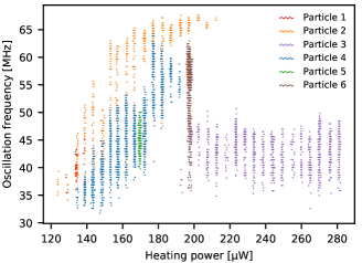
Descriptio 8: Change of the apparent oscillation frequency with heating power for different AuNPs. This figure shows the location of peaks in the Fast Fourier Transforms of individual time traces such as those shown in Fig. 5(b). Only measurements showing good oscillations are shown: those with $Q>10$, where the quality factor $Q=f_{\mathrm{max}}/\mathrm{FWHM}$ is calculated from the FFT. “Particle 4” refers to the set of measurements used in figures 5, 7 and 10.

The Fourier transforms [Fig. 5(b)] of many events show two frequencies split by a few $\mathrm{MHz}$. In real space, this corresponds to a beat note which is visible faintly in a single timetrace [e.g. Fig. 5(a)] and visibly very clearly in the mean of a series of events, shown in Fig. 5(c). Note that the timetraces in Figs. 5(c) and 5(d) are synchronized on the initial rising edge of the response, not the heating pulse, in order to eliminate the possible effect of jitter in initial explosion. The fact that the mean in Fig. 5(c) clearly shows the first few periods of the oscillation demonstrates that the oscillations are very consistently in phase from one event to the next.

The oscillations appear to only be stable between roughly $40\text{\,}\mathrm{MHz}60\text{\,}\mathrm{MHz}$. From time to time (e.g. in Fig. 7c), it looks like the resonance frequency drifts below $40\text{\,}\mathrm{MHz}$ and the oscillation collapses, before resuming later.

Oscillations manifested themselves only around some of the AuNPs tested, but were remarkably robust against changes in power—leaving aside aforementioned heating-induced damage to the AuNP. In contemplating why these oscillations might only appear some of the time, we find ourselves confronted with the question of how the oscillations are possible at all: Existing models and reports of bubble oscillation Lauterborn and Kurz (2010), including at very small scales MacDonald et al. (2003); Li et al. (2017), describe the oscillation of gas, rather than pure vapor bubbles.

Here, however, any sign of the bubble, or indeed its oscillation, disappear as soon as the heating ceases. This makes the notion of a permanent gas core in the oscillating bubbles seem unlikely. As a AuNP that supports oscillating vapor nanobubbles does so consistently—brief interruptions as seen in Fig. 7c notwithstanding—we suspect that whether any particular AuNP supports these oscillations is linked to unknown structural or geometric properties, e.g., their exact volume, the size and structure of the facets on their surfaces, or the contact area with the glass slide.

IV Conclusion

By scaling down a heating element to the nanoscale, we have, simultaneously, scaled down the classical boiling regimes, from nucleate boiling to partial and full film boiling.

The nucleate boiling regime is stunted; rapid inertially driven expansion of insulating vapor bubbles leads the system into a boiling crisis, where the absorbed power is insufficient to drive continued boiling in the presence of the newly formed vapor layer.

At higher incident powers, a boiling regime reminiscent of unstable film boiling can be sustained. Nanobubble oscillations can then be driven by the nanoheater, but for the most part, unstable boiling at the nanoscale is characterized by random fluctuations. When the laser intensity is sufficient for the AuNP to absorb and transduce a critical heat flux, even while surrounded by a thin vapor shell, vapor bubble formation stabilizes itself, leading to a nanoscale Leidenfrost effect.

Vapor nanobubble oscillations, when they occur, are remarkably consistent with the canonical model, the Rayleigh-Plesset equation, for oscillating gas bubbles of a similar size in the same environment. It would appear that, under certain conditions, vapor bubble dynamics are faster than vapor–liquid equilibration.

The transition from a highly unstable or explosive boiling regime to a stable one may have ramifications for potential applications of highly-heated nanoparticles. Mechanical stresses caused by bubble formation around gold nanoparticles, thought to be relevant in the context of plasmonic photothermal therapy Zharov et al. (2005); Huang et al. (2008); Lapotko (2011), may well be greater in an unstable boiling scenario compared to a stable one. The intuitive maxim that more laser power leads to more damage may, under these circumstances, not apply—just as the relation between heat flux and temperature in macroscopic systems has long been known to be nontrivial.

Additamentum A Approximations: Optics

The Mie-theoretical treatment of the optical properties of a multilayered sphere is exact for perfect sphere in an isotropic environment, for an incident plane-wave field.

On the first point: The nanoparticle is very nearly spherical. A transient vapor nanobubble is presumably quite spherical in order to minimize surface area. However, the environment is not isotropic in our case; the AuNP is located on a glass surface (and illuminated from below, through the glass).

On the second point: the approximately Gaussian beams are tightly focused to near the Abbe diffraction limit. For the nanoparticle itself, the finite size of the beam is negligible. When a vapor bubble approaches the size of the focus, however, the finite size of the beam will have a greater impact, further complicating the optical problem.

The straightforward treatment of the cross sections $\sigma_{\mathrm{abs}},\leavevmode\nobreak\ \sigma_{\mathrm{sca}}$ does not take into account possible (de)focusing of the beams by a nanobubble.

Additamentum B Approximations: Rayleigh-Plesset model

The Rayleigh-Plesset equation assumes the spherical bubble is composed of an ideal gas and that there is no exchange of material between the bubble and the liquid (no evaporation, condensation, dissolution, mixing, etc.). Evaporation and condensation can be included by including a vapor pressure term in the static pressure.

By not including a vapor pressure term, we are requiring full conservation of mass in the bubble. Some degree of conservation of mass is required to give rise to a restorative force and hence oscillations, as indicated above.

Lauterborn and Kurz (2010) include partial exchange of mass in their Rayleigh-Plesset equation by introducing a vapor pressure $p_{\mathrm{v}}$ that does not contribute to the pressure on the bubble wall. This is accomplished by replacing all occurrences of $p_{\mathrm{a}}$ in our Eqs. (1) and (2) with $p_{\mathrm{a}}-p_{\mathrm{v}}$. This would, all said and done, reduce the effective ambient pressure, thereby lowering the resonance frequency for any given radius. In this light, the radii derived above might be understood as rough upper bounds.

Besides the possibility of a vapor bubble with partial conservation of (vapor) mass, one might consider a mixed vapor-gas bubble. In this case, the nonvapor gas would provide the restorative force generating the mechanical resonance. However, as we point out above, we do not believe this explanation is compatible with the fact that all signs of the bubble, including the oscillations, disappear when heating ends.

It further does not take into account damping through sound radiation, any temperature dependence, or deviation from spherical symmetry. No solid gold object in the center is accounted for in the model, either. However, for a nanoparticle with $R_{\mathrm{np}}=$40\text{\,}\mathrm{nm}$$ and a bubble with $R_{\mathrm{b}}\approx$120\text{\,}\mathrm{nm}$$, the volume of the nanoparticle is less than $4\text{\,}\mathrm{\char 37\relax}$ of the bubble volume. The presence of the AuNP can therefore be neglected.

With regard to the question of why the vapor in the bubble is compressible at all, i.e., why vapor molecules do not appear to simply condense into the liquid when the bubble contracts, we can estimate the mean free path of a pentane molecule:

$$\ell=\frac{k_{\mathrm{B}}T}{\sqrt{2}\pi d^{2}p},$$

where $d$ is the molecular diameter and $p$ is the pressure. Taking $d=$0.43\text{\,}\mathrm{nm}$$ Funke et al. (1997), $T=T_{\mathrm{sat}}$ and $p=p_{\mathrm{sat}}=$1\text{\,}\mathrm{a}\mathrm{t}\mathrm{m}$+2\gamma/R$ ($\gamma$ being the surface tension at saturation Vesovic and $R=$120\text{\,}\mathrm{nm}$$ being the nanobubble radius), we get a mean free path of $\ell=$18.4\text{\,}\mathrm{nm}$$.

This is smaller than the bubble thickness, meaning that the dynamics of the molecules deep in the vapor layer are not affected by the presence of the vapor–liquid interface and it is plausible that these molecules may contribute to a restorative pressure just as foreign gas molecules would. This reasoning is not valid, of course, for the outer quarter or so of the bubble.

More broadly, this mean free path gives us a Knudsen number of order $\mathrm{Kn}\sim 10^{-1}$, confirming that a continuum hydrodynamic model like the Rayleigh-Plesset model can be applied to the bubble. For further confirmation that the continuum approximation applies, we can estimate that in an $R=$100\text{\,}\mathrm{nm}$$ sphere of a gas with $22.4\text{\,}\mathrm{L}\text{\,}{\mathrm{mol}}^{-1}$, we expect some $\sim 10^{5}$ molecules.

More complex models can include more accurate equations of state (such as a van der Waals gas law), sound radiation, and other terms Lauterborn and Kurz (2010). Lombard et al. (2015) have described a detailed model of the heat transfer problem, but even that cannot account for the optical feedback expected in the case of continuous-wave heating, touched upon in Sec. II.

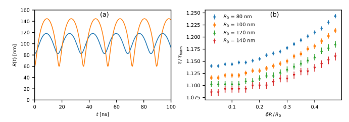
Descriptio 9: Anharmonicity of the Rayleigh-Plesset equation for a freely oscillating bubble, with the viscosity set to zero. Calculated by direct numerical (Runge–Kutta) integration with $\Delta t=$10\text{\,}\mathrm{ps}$$ using the parameters for saturated pentane. (a) Example timetraces of a bubble with $R_{0}=$120\text{\,}\mathrm{nm}$$ oscillating at two different amplitudes. The bottom of the curve, especially at larger amplitude, is noticeably more ‘pointed’, and the oscillation period is clearly different. (b) Calculated oscillation periods $\tau$ with different equilibrium radii $R_{0}$ and oscillation amplitudes $\delta R$, relative to the corresponding period $\tau_{\mathrm{harm}}$ in the harmonic approximation.

Further, our harmonic approximation drops all higher-order terms. The full equation predicts some anharmonicity at larger deviations, as shown in fig. 9. The error in the oscillation frequency predicted using the harmonic approximation at larger amplitudes is presumably small compared to the unclear effect of the driving force (due to heating) and of condensation and evaporation.

A slight anharmonicity is visible in the measured oscillations: in the series of Fourier transforms shown in fig. 10, for example, the second harmonic of the oscillation is just discernible when the Fourier transform is smoothed, or in the mean of all acquisitions. This measurement is also affected by the nonlinearity inherent in the measurement itself, as shown in fig. 2b.

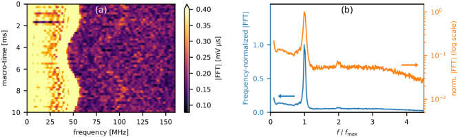
Descriptio 10: (a) Series of oscillating-bubble event Fourier transforms [same data as Fig. 7(f), smoothed with a $6\text{\,}\mathrm{MHz}$ Hann filter] showing, faintly, the second harmonic. (b) Mean of the Fourier transforms shown, calculated after rescaling the frequency axis of each to put the maximum at unity, showing clearly the second harmonic.
Note that the upper cut-off frequency of our detector is $80\text{\,}\mathrm{MHz}$, which reduces the apparent prominence of the second harmonic, and completely obscures higher harmonics.