De-Biasing The Lasso With Degrees-of-Freedom Adjustment

Abstract

This paper studies schemes to de-bias the Lasso in sparse linear regression with Gaussian design where the goal is to estimate and construct confidence intervals for a low-dimensional projection of the unknown coefficient vector in a preconceived direction $\boldsymbol{a}_{0}$. Our analysis reveals that previously analyzed propositions to de-bias the Lasso require a modification in order to enjoy nominal coverage and asymptotic efficiency in a full range of the level of sparsity. This modification takes the form of a degrees-of-freedom adjustment that accounts for the dimension of the model selected by the Lasso. The degrees-of-freedom adjustment (a) preserves the success of de-biasing methodologies in regimes where previous proposals were successful, and (b) repairs the nominal coverage and provides efficiency in regimes where previous proposals produce spurious inferences and provably fail to achieve the nominal coverage. Hence our theoretical and simulation results call for the implementation of this degrees-of-freedom adjustment in de-biasing methodologies.

Let $s_{0}$ denote the number of nonzero coefficients of the true coefficient vector and $\boldsymbol{\Sigma}$ the population Gram matrix. The unadjusted de-biasing scheme may fail to achieve the nominal coverage as soon as $s_{0}\ggg n^{2/3}$ if $\boldsymbol{\Sigma}$ is known. If $\boldsymbol{\Sigma}$ is unknown, the degrees-of-freedom adjustment grants efficiency for the contrast in a general direction $\boldsymbol{a}_{0}$ when

$$\frac{s_{0}\log p}{n}+\min\Big{\{}\frac{s_{\Omega}\log p}{n},\frac{\|\boldsymbol{\Sigma}^{-1}\boldsymbol{a}_{0}\|_{1}\sqrt{\log p}}{\|\boldsymbol{\Sigma}^{-1/2}\boldsymbol{a}_{0}\|_{2}\sqrt{n}}\Big{\}}+\frac{\min(s_{\Omega},s_{0})\log p}{\sqrt{n}}\to 0$$

where $s_{\Omega}=\|\boldsymbol{\Sigma}^{-1}\boldsymbol{a}_{0}\|_{0}$. The dependence in $s_{0},s_{\Omega}$ and $\|\boldsymbol{\Sigma}^{-1}\boldsymbol{a}_{0}\|_{1}$ is optimal and closes a gap in previous upper and lower bounds. Our construction of the estimated score vector provides a novel methodology to handle dense directions $\boldsymbol{a}_{0}$.

Beyond the degrees-of-freedom adjustment, our proof techniques yield a sharp $\ell_{\infty}$ error bound for the Lasso which is of independent interest.

MSC subject classification: 62J07 (primary), 62G15.

Key words: Statistical inference, Lasso, semiparametric model, Fisher information, efficiency, confidence interval, p-value, regression, high-dimensional data.

1 Introduction

Consider a linear regression model

$$\boldsymbol{y}=\boldsymbol{X}\boldsymbol{\beta}+{\boldsymbol{\varepsilon}}$$ (1.1)

with a sparse coefficient vector $\boldsymbol{\beta}\in{}^{p}$, a Gaussian noise vector ${\boldsymbol{\varepsilon}}\sim N({\bf 0},\sigma^{2}\boldsymbol{I}_{n})$, and a Gaussian design matrix $\boldsymbol{X}\in{}^{n\times p}$ with iid $N({\bf 0},\boldsymbol{\Sigma})$ rows. The purpose of this paper is to study the sample size requirement in de-biasing the Lasso for regular statistical inference of a linear contrast

$$\theta=\big{\langle}\boldsymbol{a}_{0},\boldsymbol{\beta}\big{\rangle}$$ (1.2)

at the $n^{-1/2}$ rate in the case of $p\gg n$ for both known and unknown $\boldsymbol{\Sigma}$. As a consequence of regularity, the $n^{-1/2}$ rate also corresponds to the length of confidence intervals for $\theta$.

The problem was considered in [Zha11] in a general semi-low-dimensional (LD) approach where high-dimensional (HD) models are decomposed as

HD model = LD component + HD component (1.3)

in the same fashion as in semi-parametric inference [BKB⁺93]. For the estimation of a real function $\theta=\theta(\boldsymbol{\beta})$ of a HD unknown parameter $\boldsymbol{\beta}$, the decomposition in (1.3) was written in the vicinity of a given $\boldsymbol{\beta}_{0}$ as

$$\boldsymbol{\beta}-\boldsymbol{\beta}_{0}=\boldsymbol{u}_{0}\big{(}\theta-\theta_{0}\big{)}+\boldsymbol{Q}_{0}\big{(}\boldsymbol{\beta}-\boldsymbol{\beta}_{0}\big{)},$$ (1.4)

where $\boldsymbol{u}_{0}$ specifies the least favorable one-dimensional local sub-model giving the minimum Fisher information for the estimation of $\theta$, subject to $\big{\langle}\boldsymbol{u}_{0},\nabla\theta(\boldsymbol{\beta}_{0})\big{\rangle}=1$, and $\boldsymbol{Q}_{0}=\boldsymbol{I}_{p\times p}-\boldsymbol{u}_{0}(\nabla\theta(\boldsymbol{\beta}_{0})){}^{\top}$ projects $\boldsymbol{\beta}-\boldsymbol{\beta}_{0}$ to a space of nuisance parameters. [Zha11] went on to propose a low-dimensional projection estimator (LDPE) as a one-step maximum likelihood correction of an initial estimator $\hat{\boldsymbol{\beta}}{}^{\text{\tiny(init)}}$ in the direction of the least favorable one-dimensional sub-model,

$$\widehat{\theta}=\theta\big{(}\hat{\boldsymbol{\beta}}{}^{\text{\tiny(init)}}\big{)}+\mathop{\rm arg\,max}_{\phi\in{\real}}\,\hbox{log-likelihood}\big{(}\hat{\boldsymbol{\beta}}{}^{\text{\tiny(init)}}+\boldsymbol{u}_{0}\phi\big{)},$$ (1.5)

and stated without proof that the asymptotic variance of such a one-step estimator achieves the lower bound given by the reciprocal of the Fisher information.

For the estimation of a contrast (1.2) in linear regression (1.1), we have $\nabla\theta(\boldsymbol{\beta}_{0})=\boldsymbol{a}_{0}$, the Fischer information in the one dimension sub-model $\{\boldsymbol{\beta}+\phi\boldsymbol{u},\phi\in{\real}\}$ is $\langle\boldsymbol{u},\boldsymbol{\Sigma}\boldsymbol{u}\rangle\sigma^{-2}$, the least favorable sub-model is given by

$$\boldsymbol{u}_{0}=\frac{\boldsymbol{\Sigma}^{-1}\boldsymbol{a}_{0}}{\langle\boldsymbol{a}_{0},\boldsymbol{\Sigma}^{-1}\boldsymbol{a}_{0}\rangle},\quad\text{i.e., the minimizer}\quad\boldsymbol{u}_{0}=\mathop{\rm arg\,min}_{\boldsymbol{u}\in{}^{p}:\langle\boldsymbol{u},\boldsymbol{a}_{0}\rangle=1}\frac{\langle\boldsymbol{u},\boldsymbol{\Sigma}\boldsymbol{u}\rangle}{\sigma^{2}}$$ (1.6)

and the Fisher information for the estimation of $\theta$ is

$$F_{\theta}=1\big{/}\left(\sigma^{2}\big{\langle}\boldsymbol{a}_{0},\boldsymbol{\Sigma}^{-1}\boldsymbol{a}_{0}\big{\rangle}\right).$$ (1.7)

In the linear model (1.1), the log-likelood function is $\boldsymbol{b}\to-\|\boldsymbol{y}-\boldsymbol{X}\boldsymbol{b}\|_{2}^{2}/(2\sigma^{2})$ up to a constant term and the one-step log-likelihood correction (1.5) can be explicitly written as a linear bias correction,

$$\widehat{\theta}=\left\langle\boldsymbol{a}_{0},\hat{\boldsymbol{\beta}}{}^{\text{\tiny(init)}}\right\rangle+\frac{\left\langle\boldsymbol{z}_{0},\boldsymbol{y}-\boldsymbol{X}\hat{\boldsymbol{\beta}}{}^{\text{\tiny(init)}}\right\rangle}{\|\boldsymbol{z}_{0}\|_{2}^{2}}\quad\text{ with }\quad\boldsymbol{z}_{0}=\boldsymbol{X}\boldsymbol{u}_{0}.$$ (1.8)

Here, $\boldsymbol{z}_{0}=\boldsymbol{X}\boldsymbol{u}_{0}$ can be viewed as an efficient score vector for the estimation of $\theta$.

In the case of unknown $\boldsymbol{\Sigma}$, the efficient score vector $\boldsymbol{z}_{0}$ has to be estimated from the data. For statistical inference of a preconceived regression coefficient $\beta_{j}$ or a linear combination of a small number of $\beta_{j}$, such one-step linear bias correction was considered in [ZZ14, BCH14, Büh13, VdGBRD14, JM14a, JM18] among others. The focus of the present paper is to find sharper sample size requirements, in the case of Gaussian design, than the typical $n\gg(s_{0}\log p)^{2}$ required in the aforementioned previous studies. Here and in the sequel,

$$s_{0}=\big{|}S\big{|}\ \hbox{ with }\ S=\operatorname{supp}(\boldsymbol{\beta}).$$ (1.9)

Our results study both known $\boldsymbol{\Sigma}$—in that case the ideal score vector $\boldsymbol{z}_{0}$ can be used—and unknown $\boldsymbol{\Sigma}$ where estimated score vectors ${\widehat{\boldsymbol{z}}}\approx\boldsymbol{z}_{0}$ are used. The results of [CG⁺17] show that for unknown $\boldsymbol{\Sigma}$ with bounded condition number, it is impossible to construct confidence intervals for $\theta=\boldsymbol{a}_{0}^{\top}\boldsymbol{\beta}$ with length of order $n^{-1/2}\|\boldsymbol{a}_{0}\|_{2}$ in the sparsity regime $s_{0}\ggg\sqrt{n}$. Proposition 4.2 in [JM18] extends the lower bound from [CG⁺17] to account for the sparsity and $\ell_{1}$ norm of $\boldsymbol{u}_{0}$ in (1.6) as follows. Let $\Theta(s_{0},s_{\Omega},\rho)$ be the collection of all pairs $(\boldsymbol{\beta},\boldsymbol{\Sigma})$ such that $\lambda_{\min}(\boldsymbol{\Sigma})^{-1}\vee\lambda_{\max}(\boldsymbol{\Sigma})\leq c_{0}$ for some absolute constant $c_{0}>1$ and

$$\|\boldsymbol{\Sigma}^{-1}\boldsymbol{e}_{j}\|_{0}\leq s_{\Omega},\qquad\|\boldsymbol{\beta}\|_{0}\leq s_{0},\qquad\|\boldsymbol{\Sigma}^{-1}\boldsymbol{e}_{j}\|_{1}\leq 1.02\vee\rho.$$

When $\boldsymbol{a}_{0}=\boldsymbol{e}_{j}$ for a fixed canonical basis vector and $s_{0}\leq c_{1}\min(p^{0.49},n/\log p)$,

$$\sup_{(\boldsymbol{\beta},\boldsymbol{\Sigma})\in\Theta(s_{0},s_{\Omega},\rho)}{\mathbb{E}}_{\boldsymbol{\beta},\boldsymbol{\Sigma}}\Big{[}n^{1/2}\sigma^{-1}|\hat{\beta}_{j}-\beta_{j}|\Big{]}\geq c_{2}+c_{3}r_{n}(s_{0},s_{\Omega},\rho)$$

with $$r_{n}(s_{0},s_{\Omega},\rho)=\min\Big{\{}{\min(s_{0},s_{\Omega})}\log(p)n^{-1/2},{(\rho\vee 1.02)}\sqrt{\log p}\Big{\}}$$

for any estimator $\hat{\beta}_{j}$ as a measurable function of $(\boldsymbol{y},\boldsymbol{X})$, where $c_{1},c_{2},c_{3}>0$ are absolute constants.

Hence the minimax rate of estimation of $\beta_{j}$ over $\Theta(s_{0},s_{\Omega},\rho)$ is at least $\sigma n^{-1/2}(1+r_{n}(s_{0},s_{\Omega},\rho))$, and any $(1-\alpha)$-confidence interval for $\beta_{j}$ valid uniformly over $\Theta(s_{0},s_{\Omega},\rho)$ must incur a length of order $\sigma n^{-1/2}(1+r_{n}(s_{0},s_{\Omega},\rho))$ up to a constant depending on $\alpha$. Since the focus of the present paper is on efficiency results and other phenomena for sparsity $s_{0}\ggg\sqrt{n}$, these impossibility results from [CG⁺17, JM18] motivate either the known $\boldsymbol{\Sigma}$ assumption (in Sections 2.1 and 3 below) or the sparsity assumptions on $\boldsymbol{\Sigma}^{-1}\boldsymbol{a}_{0}$ for unknown $\boldsymbol{\Sigma}$ in Section 2.2 where we prove that the lower bound (1) is sharp. For known $\boldsymbol{\Sigma}$, our analysis reveals that the de-biasing scheme (1.8) needs to be modified to enjoy efficiency in the regime $s_{0}\ggg n^{2/3}$ when the initial estimator is the Lasso. For unknown $\boldsymbol{\Sigma}$, the modification of (1.8) is also required for efficiency when $s_{0},s_{\Omega}$ satisfy the conditions in Theorem 2.6 of Section 2.2.

The required modification of (1.8) takes the form of a multiplicative adjustment to account for the degrees-of-freedom of the initial estimator. Interestingly, [JM14b] proved that for the Gaussian design with known $\boldsymbol{\Sigma}=\boldsymbol{I}_{p\times p}$, the sample size $n\geq Cs_{0}\log(p/s_{0})$ is sufficient in de-biasing the Lasso for the estimation of $\beta_{j}$ at the $n^{-1/2}$ rate. More recently, [JM18] extended this result and showed that $n\geq Cs_{0}(\log p)^{2}$ is sufficient to de-bias the Lasso for the estimation of $\beta_{j}$ at the $n^{-1/2}$ rate for Gaussian designs with known covariance matrices $\boldsymbol{\Sigma}$ when the $\ell_{1}$ norm of each column of $\boldsymbol{\Sigma}^{-1}$ is bounded, i.e., for some constant $\rho>0$

$$\max_{j=1,...,p}\|\boldsymbol{\Sigma}^{-1}\boldsymbol{e}_{j}\|_{1}\leq\rho$$ (1.11)

holds, where $(\boldsymbol{e}_{1},...,\boldsymbol{e}_{p})$ is the canonical basis in ^p. From this perspective, the present paper provides an extension of these results to more general $\boldsymbol{\Sigma}$: We will see below that for $n\geq Cs_{0}\log(p)^{2}$, the efficiency of the de-biasing scheme (1.8) is specific to assumption (1.11) and that the de-biasing scheme (1.8) requires a modification to be efficient in cases where (1.11) is violated.

The paper is organized as follows. Section 2 provides a description of our proposed estimator, which is a modification of the de-biasing scheme (1.8) that accounts for the degrees-of-freedom of the initial estimator. Section 3 describes our strongest results in linear regression with known covariance matrix for the Lasso. This includes several efficiency results for the de-biasing scheme modified with degrees-of-freedom adjustment and a characterization of the asymptotic regime where this adjustment is necessary. Section 4 studies the specific situation where bounds on the $\ell_{1}$ norm of $\boldsymbol{\Sigma}^{-1}\boldsymbol{a}_{0}$ are available, similarly to (1.11) when $\boldsymbol{a}_{0}$ is a canonical basis vector. The additional assumptions on $\boldsymbol{\Sigma}^{-1}$ and the results of Section 4 explain why the necessity of degrees-of-freedom adjustment did not appear in some previous works. Section 5 provides a new $\ell_{\infty}$ bound for estimation of $\boldsymbol{\beta}$ by the Lasso under assumptions similar to (1.11). Section 6 discusses efficiency and regularity, and shows that asymptotic normality remains unchanged under non-sparse $n^{-1/2}$-perturbations of $\boldsymbol{\beta}$. Section 7 shows that the degrees-of-freedom adjustment is also needed for certain non-Gaussian designs. The proofs of the main results are given in Sections 8, A, B and H. The proofs of intermediary lemmas and propositions can be found in Appendices D, E, F and G. Our main technical tool is a carefully constructed Gaussian interpolation path described in Section 8.1.

Notation

We use the following notation throughout the paper. Let $\boldsymbol{I}_{d}$ be the identity matrix of size $d\times d$, e.g. $d=n,p$. For any $p\geq 1$, let $[p]$ be the set $\{1,...,p\}$. For any vector $\boldsymbol{v}=(v_{1},...,v_{p})^{\top}\in{}^{p}$ and any set $A\subset[p]$, the vector $\boldsymbol{v}_{A}\in{}^{|A|}$ is the restriction $(v_{j})_{j\in A}$. For any $n\times p$ matrix $\boldsymbol{M}$ with columns $(\boldsymbol{M}_{1},\ldots,\boldsymbol{M}_{p})$ and any subset $A\subset[p]$, let $\boldsymbol{M}_{A}=(\boldsymbol{M}_{j},j\in A)$ be the matrix composed of columns of $\boldsymbol{M}$ indexed by $A$, and $\boldsymbol{M}_{A}^{\dagger}$ be the Moore-Penrose generalized inverse of $\boldsymbol{M}_{A}$. If $\boldsymbol{M}$ is a symmetric matrix of size $p\times p$ and $A\subset[p]$, then $\boldsymbol{M}_{A,A}$ denotes the sub-matrix of $\boldsymbol{M}$ with rows and columns in $A$, and $\boldsymbol{M}_{A,A}^{-1}$ is the inverse of $\boldsymbol{M}_{A,A}$. Let $\|\cdot\|_{q}$ denote the $\ell_{q}$ norm of vectors, $\|\cdot\|_{op}$ the operator norm (largest singular value) of matrices and $\|\cdot\|_{F}$ the Frobenius norm. We use the notation $\langle\cdot,\cdot\rangle$ for the canonical scalar product of vectors in ⁿ or ^p, i.e., $\langle\boldsymbol{a},\boldsymbol{b}\rangle=\boldsymbol{a}^{\top}\boldsymbol{b}$ for two vectors $\boldsymbol{a},\boldsymbol{b}$ of the same dimension.

Throughout the paper, $C_{0}=\|\boldsymbol{\Sigma}^{-1/2}\boldsymbol{a}_{0}\|_{2}$, $\boldsymbol{u}_{0}$ is as in (1.6) and $F_{\theta}$ as in (1.7). The score vector $\boldsymbol{z}_{0}$ is always defined as $\boldsymbol{z}_{0}=\boldsymbol{X}\boldsymbol{u}_{0}$ and $\boldsymbol{Q}_{0}$ is the matrix $\boldsymbol{Q}_{0}=\boldsymbol{I}_{p\times p}-\boldsymbol{u}_{0}\boldsymbol{a}_{0}^{\top}$, so that

$$\boldsymbol{X}=\boldsymbol{X}\boldsymbol{Q}_{0}+\boldsymbol{z}_{0}\boldsymbol{a}_{0}^{\top}$$

always holds. As in (1.9), $S$ and $s_{0}$ are the support and number of nonzero coefficients of the unknown coefficient vector $\boldsymbol{\beta}$. For any event $\Omega$, denote by $I_{\Omega}$ its indicator function and $a_{+}=\max(0,a)$ for $a\in{\real}$.

2 Degrees of freedom adjustment

2.1 Known $\boldsymbol{\Sigma}$

In addition to the de-biasing scheme (1.8), we consider the following degrees-of-freedom adjusted version of it. Suppose that the Lasso estimator $\hat{\boldsymbol{\beta}}{}^{\text{\tiny(lasso)}}$ is used as the initial estimator $\hat{\boldsymbol{\beta}}{}^{\text{\tiny(init)}}$, where

$$\hat{\boldsymbol{\beta}}{}^{\text{\tiny(lasso)}}=\mathop{\rm arg\,min}_{\boldsymbol{b}\in{}^{p}}\left\{\|\boldsymbol{y}-\boldsymbol{X}\boldsymbol{b}\|_{2}^{2}/(2n)+\lambda\|\boldsymbol{b}\|_{1}\right\}.$$ (2.1)

The degrees-of-freedom adjusted LDPE is defined as

$$\widehat{\theta}_{\nu}=\left\langle\boldsymbol{a}_{0},\hat{\boldsymbol{\beta}}{}^{\text{\tiny(lasso)}}\right\rangle+\frac{\left\langle\boldsymbol{z}_{0},\boldsymbol{y}-\boldsymbol{X}\hat{\boldsymbol{\beta}}{}^{\text{\tiny(lasso)}}\right\rangle}{\|\boldsymbol{z}_{0}\|_{2}^{2}(1-\nu/n)},$$ (2.2)

where $\boldsymbol{z}_{0}$ is as in (1.8) and $\nu\in[0,n)$ is a degrees-of-freedom adjustment; $\nu$ is allowed to be random. Our theoretical results will justify the degrees-of-freedom adjustment $\nu=|{\widehat{S}}|$ where ${\widehat{S}}=\operatorname{supp}(\hat{\boldsymbol{\beta}}{}^{\text{\tiny(lasso)}})$. The size of the selected model has the interpretation of degrees of freedom for the Lasso estimator in the context of Stein’s Unbiased Risk Estimate (SURE) [ZHT07, Zha10, TT12].

We still retain other possibilities for $\nu$ such as $\nu=0$ in order to analyse the unadjusted de-biasing scheme (1.8). With some abuse of notation, in order to avoid any ambiguity we may sometimes use the notation $\widehat{\theta}_{\nu=0}$ for the unadjusted (1.8) and $\widehat{\theta}{}_{\nu=|{\widehat{S}}|}$ for (2.2) with $|{\widehat{S}}|$ being the size of the support of the Lasso.

Our main results will be developed in Section 3. Here is a simpler version of the story.

Theorem 2.1.

Let $s_{0},n$ and $p$ be positive integers satisfying $p/s_{0}\to\infty$ and $(s_{0}/n)\log(p/s_{0})\to 0$. Assume that $\boldsymbol{\Sigma}_{jj}\leq 1$ for all $j\in[p]$ and that the spectrum of $\boldsymbol{\Sigma}$ is uniformly bounded away from 0 and $\infty$; e.g. $\max(\|\boldsymbol{\Sigma}\|_{op},\|\boldsymbol{\Sigma}^{-1}\|_{op})\leq 2$. Let $\lambda=1.01\sigma\sqrt{2\log(8p/s_{0})/n}$.

(i) Then $|{\widehat{S}}|=O_{{\mathbb{P}}}(s_{0})=o_{{\mathbb{P}}}(n)$ and for $\nu=|{\widehat{S}}|$ we have for every $\boldsymbol{a}_{0}$

$$\sqrt{nF_{\theta}}\left(1-|{\widehat{S}}|/n\right)\left(\widehat{\theta}_{\nu=|{\widehat{S}}|}-\theta\right)=T_{n}+o_{\mathbb{P}}(1)$$ (2.3)

where $T_{n}=\sqrt{nF_{\theta}}\langle\boldsymbol{z}_{0},{\boldsymbol{\varepsilon}}\rangle/\|\boldsymbol{z}_{0}\|_{2}^{2}$ has the $t$-distribution with $n$ degrees of freedom. Thus the estimator (2.2) enjoys asymptotic efficiency when $\nu=|{\widehat{S}}|$.

(ii) The quantity $\sqrt{nF_{\theta}}(\widehat{\theta}_{\nu=0}-\theta)-T_{n}$ is unbounded for certain $\boldsymbol{\beta}$ satisfying $n/\log(p/s_{0})\ggg s_{0}\ggg n^{2/3}/\log(p/s_{0})^{1/3}$ and $\boldsymbol{a}_{0}$ depending on $S$ and $\boldsymbol{\Sigma}$ only. Consequently, the unadjusted (1.8) cannot be efficient.

Theorem 2.1(ii) implies that with $\nu=0$, the unadjusted (1.8) cannot be efficient in the whole range $\{s_{0}:s_{0}\log(p/s_{0})\lll n\}$ of sparsity levels unless extra assumptions are made on the covariance matrix $\boldsymbol{\Sigma}$ such as (1.11). Theorem 2.1(i) shows that using the adjustment $\nu=|{\widehat{S}}|$ repairs this: The efficiency in (2.3) then holds in the whole range $\{s_{0}:s_{0}\log(p/s_{0})\lll n\}$ of sparsity levels. Theorem 2.1(i) is proved after Corollary 3.2 below while (ii) is a consequence of the following proposition.

Proposition 2.2.

Let the setting and assumptions of Theorem 2.1 be fulfilled and let $\nu$ be a random variable with $\nu\in[0,n)$ almost surely. Then

$$\sqrt{nF_{\theta}}(\widehat{\theta}_{\nu}-\theta) = T_{n}+o_{\mathbb{P}}(1)+n^{-1}(\nu-|{\widehat{S}}|)\Lambda_{\nu}$$ (2.4)

where $\Lambda_{\nu}=\sqrt{nF_{\theta}}(1-\nu/n)^{-1}(1-|{\widehat{S}}|/n)^{-1}\|\boldsymbol{z}_{0}\|^{-2}\langle\boldsymbol{z}_{0},\boldsymbol{y}-\boldsymbol{X}{\hat{\boldsymbol{\beta}}{}^{\text{\tiny(lasso)}}}\rangle.$ Furthermore for any $(s_{\Omega},s_{0})$ with $s_{\Omega}\leq s_{0}=o(n/\log(p/s_{0}))$, and any $\boldsymbol{a}_{0}$ with $\|\boldsymbol{\Sigma}^{-1/2}\boldsymbol{a}_{0}\|_{2}=1$ and $\|\boldsymbol{\Sigma}^{-1}\boldsymbol{a}_{0}\|_{0}=s_{\Omega}$, there exists $\boldsymbol{\beta}$ with $\|\boldsymbol{\beta}\|_{0}=s_{0}$ such that

$${\mathbb{P}}\bigl{[}|\Lambda_{\nu}|\geq\|\boldsymbol{\Sigma}^{-1}\boldsymbol{a}_{0}\|_{1}\sqrt{\log(8p/s_{0})}\bigr{]}\to 1,\quad{\mathbb{P}}\bigl{[}|{\widehat{S}}|\geq s_{0}\bigr{]}\to 1.$$ (2.5)

In particular, it is possible to pick $\boldsymbol{a}_{0}$ satisfying in addition $\|\boldsymbol{\Sigma}^{-1}\boldsymbol{a}_{0}\|_{1}\geq s_{\Omega}^{1/2}/\|\boldsymbol{\Sigma}\|_{op}^{1/2}$.

Proposition 2.2 is proved in Appendix C. Theorem 2.1(ii) is implied by Proposition 2.2 with $s_{\Omega}=s_{0}$: If $s_{0}^{3/2}\sqrt{\log(8p/s_{0})}/n\to+\infty$ then $n^{-1}|{\widehat{S}}|\Lambda_{\nu=0}$ is unbounded with probability approaching one by (2.5), while the other terms in (2.4) are stochastically bounded.

Example 2.1.

It is informative to unpack from the proof of Proposition 2.2 how $(\boldsymbol{a}_{0},\boldsymbol{u}_{0},\boldsymbol{\beta})$ is constructed so that (2.5) holds. Theorem 2.1 and Proposition 2.2 apply to any $\boldsymbol{\Sigma}$ with bounded spectrum and $\Sigma_{ii}\leq 1$. Let $\boldsymbol{\beta}$ be an $s_{0}$-sparse vector with large enough non-zero coefficients and $\beta_{j}>0$ for some index $j=1,...,p$ that is fixed throughout this example. Then let $\boldsymbol{v}\in\{-1,0,1\}^{p}$ be an $s_{\Omega}$-sparse vector with $\operatorname{supp}(\boldsymbol{v})\subset\operatorname{supp}(\boldsymbol{\beta})$ and $v_{k}=\hbox{\rm sgn}(\beta_{k})$ for all $k\in\operatorname{supp}(\boldsymbol{v})$. Consider

$$\boldsymbol{\Omega}=\boldsymbol{I}_{p}+(1/4)s_{\Omega}^{-1/2}[\boldsymbol{e}_{j}\boldsymbol{v}^{\top}+\boldsymbol{v}\boldsymbol{e}_{j}^{\top}].$$

which has bounded spectrum since $\|\boldsymbol{\Omega}-\boldsymbol{I}_{p}\|_{op}\leq 1/2$ and set $\boldsymbol{\Sigma}=\boldsymbol{\Omega}^{-1}\kappa$ for some constant $\kappa>0$ such that $\max_{j=1,...,p}\Sigma_{jj}=1$. Since $\boldsymbol{\Omega}$ has bounded spectrum, $\kappa$ is also bounded and the spectrum of $\boldsymbol{\Sigma}$ is bounded as required. From the proof of Proposition 2.2, we see that the requirement for $\boldsymbol{u}_{0}$ is that

$$\langle\boldsymbol{u}_{0},\hbox{\rm sgn}(\boldsymbol{\beta})\rangle=\|\boldsymbol{u}_{0}\|_{1}$$ (2.6)

must hold. For the $\boldsymbol{\Sigma}$ just defined, set $\boldsymbol{u}_{0}=\boldsymbol{\Omega}\boldsymbol{e}_{j}=\bigl{(}1+(1/4)s_{\Omega}^{-1/2}v_{j}\bigr{)}\boldsymbol{e}_{j}+(1/4)s_{\Omega}^{-1/2}\boldsymbol{v}$. Since $\boldsymbol{\beta}$ was chosen with $\beta_{j}>0$, we have $v_{j}\geq 0$ by definition of $\boldsymbol{v}$ and $\boldsymbol{u}_{0}$ satisfies (2.6). These quantities $(\boldsymbol{\Sigma},\boldsymbol{\beta},\boldsymbol{u}_{0})$, when $\boldsymbol{\beta}$ has large enough coefficients, satisfy (2.5) by the proof of Proposition 2.2. Finally, from (1.6) there is a one-to-one correspondence between $\boldsymbol{u}_{0}$ and $\boldsymbol{a}_{0}$ given by $\boldsymbol{a}_{0}=\boldsymbol{\Sigma}\boldsymbol{u}_{0}/\langle\boldsymbol{u}_{0},\boldsymbol{\Sigma}\boldsymbol{u}_{0}\rangle$. This implies $\boldsymbol{a}_{0}=\boldsymbol{\Omega}^{-1}\boldsymbol{u}_{0}/\langle\boldsymbol{u}_{0},\boldsymbol{\Omega}^{-1}\boldsymbol{u}_{0}\rangle$ and since $\boldsymbol{u}_{0}=\boldsymbol{\Omega}\boldsymbol{e}_{j}$, the direction $\boldsymbol{a}_{0}$ for this example is proportional to the canonical basis vector $\boldsymbol{e}_{j}$. Proposition 2.2 thus proves the necessity of the degrees-of-freedom adjustment with $\boldsymbol{a}_{0}$ proportional to $\boldsymbol{e}_{j}$. Figure 2 illustrates this phenomenon on simulated data.

The adjustment in (2.2) was proposed by [JM14b] in the form of

$$\hat{\boldsymbol{\beta}}=\hat{\boldsymbol{\beta}}{}^{\text{\tiny(lasso)}}+\frac{\boldsymbol{\Sigma}^{-1}\boldsymbol{X}^{\top}(\boldsymbol{y}-\boldsymbol{X}\hat{\boldsymbol{\beta}}{}^{\text{\tiny(lasso)}})}{n-\nu}$$ (2.7)

based on heuristics of the replica method from statistical physics and a theoretical justification in the case of $\boldsymbol{\Sigma}=\boldsymbol{I}_{p}$. As $\boldsymbol{z}_{0}=\boldsymbol{X}\boldsymbol{u}_{0}$ with $\boldsymbol{u}_{0}=\boldsymbol{\Sigma}^{-1}\boldsymbol{a}_{0}/\big{\langle}\boldsymbol{a}_{0},\boldsymbol{\Sigma}^{-1}\boldsymbol{a}_{0}\big{\rangle}$ in (1.8), ${\mathbb{E}}\|\boldsymbol{z}_{0}\|_{2}^{2}/n=1/\big{\langle}\boldsymbol{a}_{0},\boldsymbol{\Sigma}^{-1}\boldsymbol{a}_{0}\big{\rangle}$ and

$$\frac{\left\langle\boldsymbol{z}_{0},\boldsymbol{y}-\boldsymbol{X}\hat{\boldsymbol{\beta}}{}^{\text{\tiny(init)}}\right\rangle}{\big{(}{\mathbb{E}}\|\boldsymbol{z}_{0}\|_{2}^{2}\big{)}(1-\nu/n)}=\left\langle\boldsymbol{a}_{0},\frac{\boldsymbol{\Sigma}^{-1}\boldsymbol{X}^{\top}(\boldsymbol{y}-\boldsymbol{X}\hat{\boldsymbol{\beta}}{}^{\text{\tiny(lasso)}})}{n-\nu}\right\rangle.$$

Thus, the plug-in estimator

$$\widehat{\theta}_{\nu}=\left\langle\boldsymbol{a}_{0},\hat{\boldsymbol{\beta}}\right\rangle\ \hbox{with the $\hat{\boldsymbol{\beta}}$ in (\ref{est-JM})},$$ (2.8)

is equivalent to replacing $\|\boldsymbol{z}_{0}\|_{2}^{2}$ with its expectation in the denominator of the bias correction term in (2.2). Another version of the estimator, akin to the version of the LDPE proposed in [ZZ14], is

$$\widehat{\theta}_{\nu}=\left\langle\boldsymbol{a}_{0},\hat{\boldsymbol{\beta}}{}^{\text{\tiny(lasso)}}\right\rangle+\frac{\left\langle\boldsymbol{z}_{0},\boldsymbol{y}-\boldsymbol{X}\hat{\boldsymbol{\beta}}{}^{\text{\tiny(lasso)}}\right\rangle}{\big{\langle}\boldsymbol{z}_{0},\boldsymbol{X}\boldsymbol{u}\big{\rangle}(1-\nu/n)}$$ (2.9)

with a vector $\boldsymbol{u}\in{}^{p}$ satisfying $\langle\boldsymbol{u},\boldsymbol{a}_{0}\rangle=1$. Since ${\mathbb{E}}\big{\langle}\boldsymbol{z}_{0},{\boldsymbol{X}\boldsymbol{u}}\big{\rangle}={\mathbb{E}}\|\boldsymbol{z}_{0}\|_{2}^{2}$, the estimator (2.7) also corresponds to (2.9) with $\langle\boldsymbol{z}_{0},{\boldsymbol{X}\boldsymbol{u}}\rangle$ replaced by its expectation in the denominator of the bias correction term.

Let $\boldsymbol{h}{}^{\text{\tiny(lasso)}}=(\hat{\boldsymbol{\beta}}{}^{\text{\tiny(lasso)}}-\boldsymbol{\beta})$. It is worthwhile to mention here that when $\|\boldsymbol{X}\boldsymbol{h}{}^{\text{\tiny(lasso)}}\|_{2}/\sqrt{n}=o_{\mathbb{P}}(1)$ based on existing results on the Lasso, the asymptotic distribution of (2.2) adjusted at the $n^{-1/2}$ rate does not change when $\|\boldsymbol{z}_{0}\|_{2}^{2}$ is replaced by a quantity of type $\|\boldsymbol{z}_{0}\|_{2}^{2}(1+O(n^{-1/2}))$ in the denominator of the bias correction term. Indeed,

$$\sqrt{nF_{\theta}}\bigg{|}\frac{\left\langle\boldsymbol{z}_{0},\boldsymbol{y}-\boldsymbol{X}\hat{\boldsymbol{\beta}}{}^{\text{\tiny(lasso)}}\right\rangle}{\|\boldsymbol{z}_{0}\|_{2}^{2}(1-\nu/n)}-\frac{\left\langle\boldsymbol{z}_{0},\boldsymbol{y}-\boldsymbol{X}\hat{\boldsymbol{\beta}}{}^{\text{\tiny(lasso)}}\right\rangle}{\|\boldsymbol{z}_{0}\|_{2}^{2}(1+O(n^{1/2}))(1-\nu/n)}\bigg{|}$$

$$\leq O(1)(1-\nu/n)^{-1}\left(|T_{n}|n^{-1/2}+\|\boldsymbol{X}\boldsymbol{h}{}^{\text{\tiny(lasso)}}\|_{2}/(\sigma C_{0}\|\boldsymbol{z}_{0}\|_{2})\right).$$

The right-hand side converges to 0 in probability if $(1-\nu/n)^{-1}=O_{\mathbb{P}}(1)$ and $\|\boldsymbol{X}\boldsymbol{h}{}^{\text{\tiny(lasso)}}\|_{2}/\sqrt{n}=o_{\mathbb{P}}(1)$ since $T_{n}$ has the $t$-distribution with $n$ degrees of freedom. Thus, as (2.2), (2.8) and (2.9) are asymptotically equivalent, the most notable feature of these estimators is the degrees-of-freedom adjustment with the choice $\nu=|{\widehat{S}}|$, as proposed in [JM14b], compared with earlier proposals with $\nu=0$. While the properties of these estimators for general $\boldsymbol{\beta}$ and $\boldsymbol{\Sigma}$ will be studied in the next section, we highlight in the following theorem the requirement of either a degrees-of-freedom adjustment or some extra condition on the bias of the Lasso in the special case where the Lasso is sign consistent.

Theorem 2.3.

Suppose that the Lasso is sign consistent in the sense of

$${\mathbb{P}}\Big{\{}\hbox{\rm sgn}(\hat{\boldsymbol{\beta}}{}^{\text{\tiny(lasso)}})=\hbox{\rm sgn}(\boldsymbol{\beta})\Big{\}}\to 1.$$ (2.11)

Let $C_{0}=\|\boldsymbol{\Sigma}^{-1/2}\boldsymbol{a}_{0}\|_{2}$ and $C_{\boldsymbol{\beta}}=\|\boldsymbol{\Sigma}_{S,S}^{-1/2}\hbox{\rm sgn}(\boldsymbol{\beta}_{S})\|_{2}/\sqrt{s_{0}}$. Suppose that $\sqrt{(1\vee s_{0})/n}+C_{\boldsymbol{\beta}}\sqrt{s_{0}}(\lambda/\sigma)\big{)}\leq\eta_{n}$ for a sufficiently small $\eta_{n}<1$. Let $F_{\theta}=1/(\sigma C_{0})^{2}$ be the Fisher information as in (1.7), and $T_{n}=\sqrt{nF_{\theta}}\langle\boldsymbol{z}_{0},{\boldsymbol{\varepsilon}}\rangle/\|\boldsymbol{z}_{0}\|_{2}^{2}$ so that $T_{n}$ has the $t$-distribution with $n$ degrees of freedom. Let $\widehat{\theta}_{\nu}$ be as in (2.2) or (2.8). Then,

$$(1-\nu/n)\sqrt{nF_{\theta}}\big{(}\widehat{\theta}_{\nu}-\theta\big{)}=T_{n}+O_{{\mathbb{P}}}(\eta_{n})$$ (2.12)

for a random variable $\nu\in[0,s_{0}]$ if and only if

$$\sqrt{F_{\theta}/n}\big{(}s_{0}-\nu\big{)}\big{\langle}\boldsymbol{a}_{0},\hat{\boldsymbol{\beta}}{}^{\text{\tiny(lasso)}}-\boldsymbol{\beta}\big{\rangle}=O_{{\mathbb{P}}}(\eta_{n}),$$ (2.13)

if and only if

$$\sqrt{F_{\theta}/n}\big{(}s_{0}-\nu\big{)}\big{\langle}(\boldsymbol{a}_{0})_{S},\lambda(\boldsymbol{X}_{S}^{\top}\boldsymbol{X}_{S}/n)^{-1}\hbox{\rm sgn}(\boldsymbol{\beta}_{S})\big{\rangle}=O_{{\mathbb{P}}}(\eta_{n}).$$ (2.14)

The conclusion also holds for the $\widehat{\theta}_{\nu}$ in (2.9) when $C_{0}\|\boldsymbol{\Sigma}^{1/2}\boldsymbol{u}\|_{2}=O(1)$.

The proof is given in Appendix H. Theorem 2.3 provides an alternative negative result, similar in flavor to Theorem 2.1(ii) and Proposition 2.2 above. The settings may not match exactly since the tuning parameter $\lambda$ required for sign consistency is larger than the one featured in Theorem 2.1. Compared with Proposition 2.2, the sign consistency lets us derive the two explicit conditions (2.13)-(2.14) for efficiency that are useful to pinpoint situations, such as those described in the next two paragraphs, where efficiency does not hold.

Theorem 2.3 implies that for efficient statistical inference of $\theta$ at the $n^{-1/2}$ rate, the unadjusted de-biasing scheme (1.8) requires either a degrees-of-freedom adjustment or the extra condition that the bias of the initial Lasso estimator of $\theta$, given by $\big{\langle}(\boldsymbol{a}_{0})_{S},\lambda(\boldsymbol{X}_{S}^{\top}\boldsymbol{X}_{S}/n)^{-1}\hbox{\rm sgn}(\boldsymbol{\beta}_{S})\big{\rangle}$, is of order $o_{{\mathbb{P}}}(n^{1/2}/s_{0})$, even when the initial Lasso estimator is sign-consistent. For example, if $(\boldsymbol{a}_{0})_{S^{c}}=0$ and $(\boldsymbol{a}_{0})_{S}=\hbox{\rm sgn}(\boldsymbol{\beta}_{S})/\|\boldsymbol{\Sigma}^{-1/2}\hbox{\rm sgn}(\boldsymbol{\beta}_{S})\|_{2}$, then $\boldsymbol{a}_{0}$ is standardized with $\|\boldsymbol{\Sigma}^{-1/2}\boldsymbol{a}_{0}\|_{2}=1$ and condition (2.14) on the bias can be written as

$$(\lambda/\sigma)n^{-1/2}(s_{0}-\nu)\|\boldsymbol{\Sigma}_{S,S}^{-1/2}\hbox{\rm sgn}(\boldsymbol{\beta}_{S})\|_{2}=O_{\mathbb{P}}(\eta_{n})$$

because the singular values of the Wishart matrix $\boldsymbol{\Sigma}_{S,S}^{-1/2}(\boldsymbol{X}_{S}^{\top}\boldsymbol{X}_{S}/n)\boldsymbol{\Sigma}_{S,S}^{-1/2}$ are bounded away from 0 and $+\infty$ with high probability. For $\nu=0$, this is equivalent to $C_{\boldsymbol{\beta}}(\lambda/\sigma)s_{0}^{3/2}/\sqrt{n}=O(\eta_{n})$. If $C_{\boldsymbol{\beta}}$ is of order of a constant and $\eta_{n}<1$, this implies that the unadjusted de-biasing scheme (1.8) cannot be efficient in the asymptotic regime when

$$(\lambda/\sigma)s_{0}^{3/2}/\sqrt{n}\ggg 1.$$ (2.15)

Interestingly, the condition $(\lambda/\sigma)s_{0}^{3/2}/\sqrt{n}=O(1)$ is weaker than the typical sample size requirement $n\gg(s_{0}\log p)^{2}$ in the case of unknown $\boldsymbol{\Sigma}$.

Another enlightening situation is $\boldsymbol{a}_{0}=\boldsymbol{e}_{j}$ the $j$-th canonical basis vector for some $j\in S$, $S=\{1,...,s_{0}\}$ and $\boldsymbol{\Sigma}^{-1}$ diagonal by block with two blocks

$$\boldsymbol{\Sigma}^{-1}=\begin{pmatrix}\boldsymbol{I}_{|S|}+(1/4)|S|^{-1/2}[\hbox{\rm sgn}(\boldsymbol{\beta}_{S})\boldsymbol{e}_{j}^{\top}+\boldsymbol{e}_{j}\hbox{\rm sgn}(\boldsymbol{\beta}_{S})^{\top}]&\mathbf{0}_{|S|,p-|S|}\\ \mathbf{0}_{p-|S|,|S|}&\boldsymbol{I}_{p-|S|}\end{pmatrix}.$$

The eigenvalues of $\boldsymbol{\Sigma}^{-1/2}$ belong to $[1/2,3/2]$ by construction since $(|S|)^{-1/2}\hbox{\rm sgn}(\boldsymbol{\beta}_{S})\boldsymbol{e}_{j}^{\top}$ has operator norm equal to one. Again using properties of the singular values of the Wishart matrix $\boldsymbol{\Sigma}_{S,S}^{-1/2}(\boldsymbol{X}_{S}^{\top}\boldsymbol{X}_{S}/n)\boldsymbol{\Sigma}_{S,S}^{-1/2}$, the left hand-side of condition (2.14) is of order

$$\sqrt{F_{\theta}/n}(s_{0}-\nu)\lambda\boldsymbol{e}_{j}^{\top}(\boldsymbol{\Sigma}_{S,S})^{-1}\hbox{\rm sgn}(\boldsymbol{\beta}_{S})\asymp(\lambda/\sigma)n^{-1/2}(s_{0}-\nu)\sqrt{s_{0}}.$$

Similarly to the previous paragraph, this implies that with $\nu=0$ the unadjusted de-biasing scheme (1.8) cannot be efficient if (2.15) holds. Up to a multiplicative constant in $\boldsymbol{\Sigma}$, this example is similar to Example 2.1 with $s_{\Omega}=s_{0}$.

The novelty of our contributions resides in the $s_{0}^{2}\ggg n$ regime up to logarithmic factor, in the sparsity range where the transition (2.15) happens. The necessity of the degrees-of-freedom adjustment can be seen in simulated data as follows. Figure 1 presents the distribution of $\sqrt{n}(\hat{\theta}_{\nu}-\theta)$ with and without the adjustment for $\boldsymbol{\Sigma}=\boldsymbol{I}_{p},\sigma=1$ for $(n,p)=(4000,6000)$ and $s_{0}=20,40,80,120$. Although classical results on de-biasing in the regime $s_{0}^{2}\lll n$ proves that $\sqrt{n}(\hat{\theta}_{\nu}-\theta)\approx N(0,1)$ [ZZ14, JM14a, VdGBRD14] with $\nu=0$, simulations reveal that $\sqrt{n}(\hat{\theta}_{\nu}-\theta)$ is substantially biased (downward in Figure 1), and any confidence interval constructed from $\sqrt{n}(\hat{\theta}_{\nu}-\theta)\approx N(0,1)$ would not correctly control Type-I error due to this substantial bias. This substantial bias is present for sparsity as small as $s_{0}=20$ (for which $s_{0}^{2}/n=0.1$). On the other hand, the adjustment $\nu=|{\widehat{S}}|$ repairs this, as shown both in the simulation in Figure 1 and by the theory in Theorem 2.1 and in the next sections. Thus our novel results on the necessity of the degrees-of-freedom adjustment is not only theoretical; It also explains the gap between simulations and the predictions from the early literature on de-biasing [ZZ14, JM14a, VdGBRD14] where the degrees-of-freedom adjustment is absent.

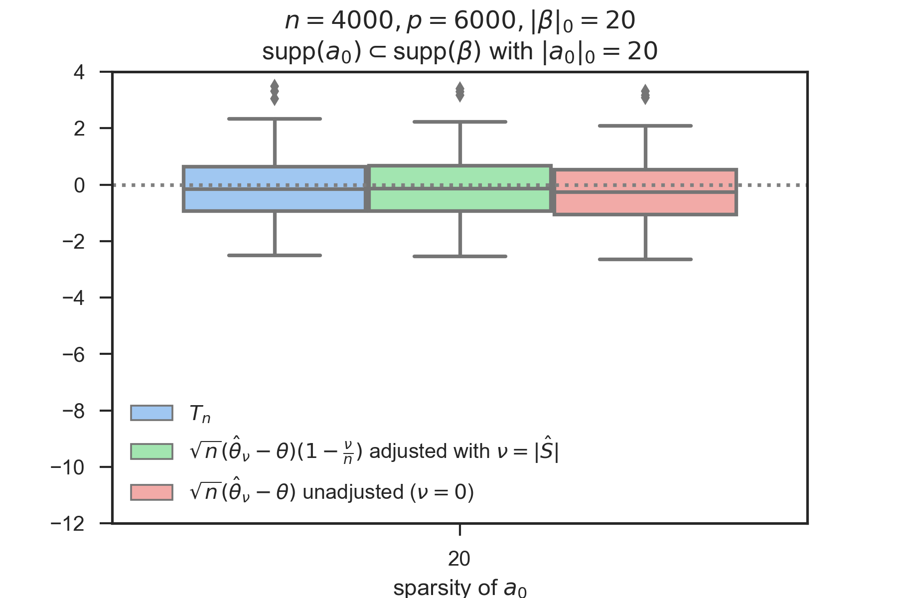
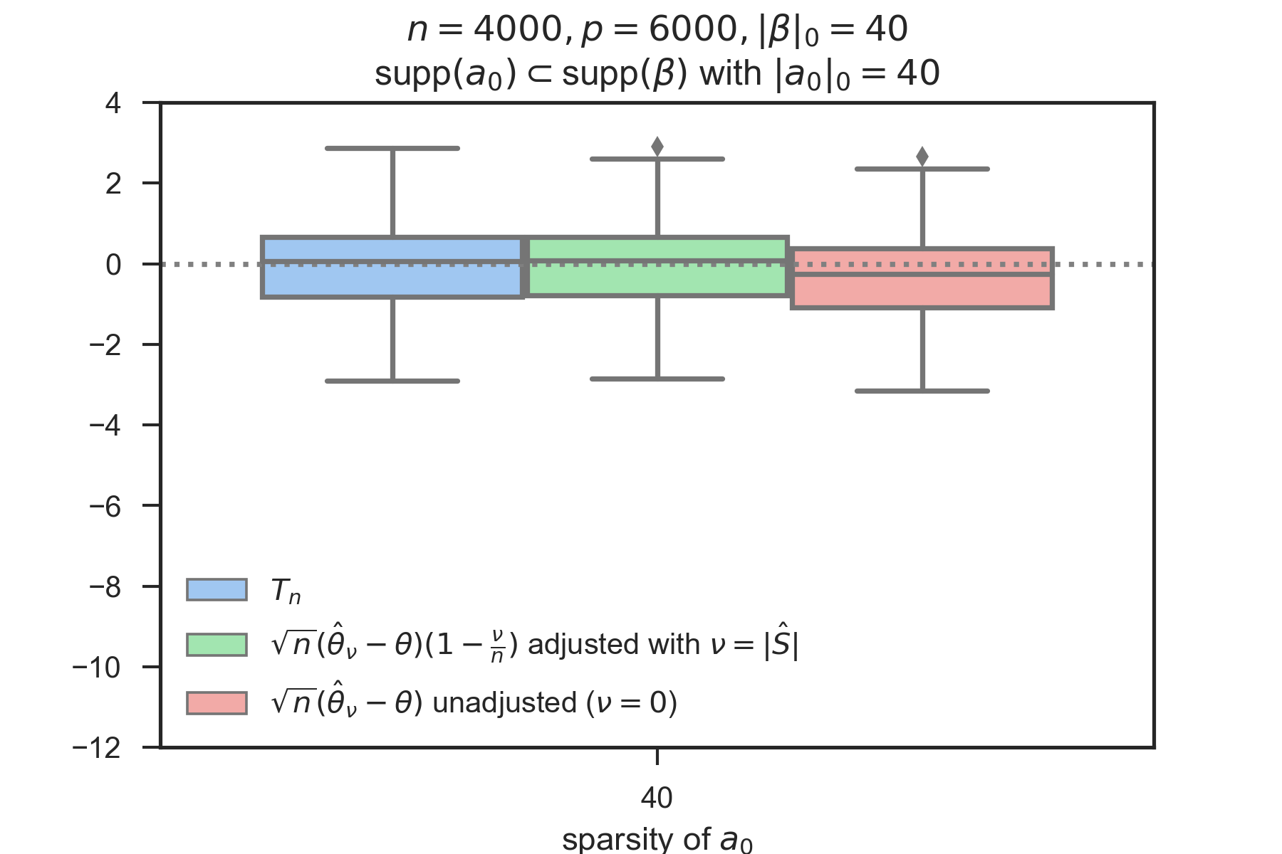
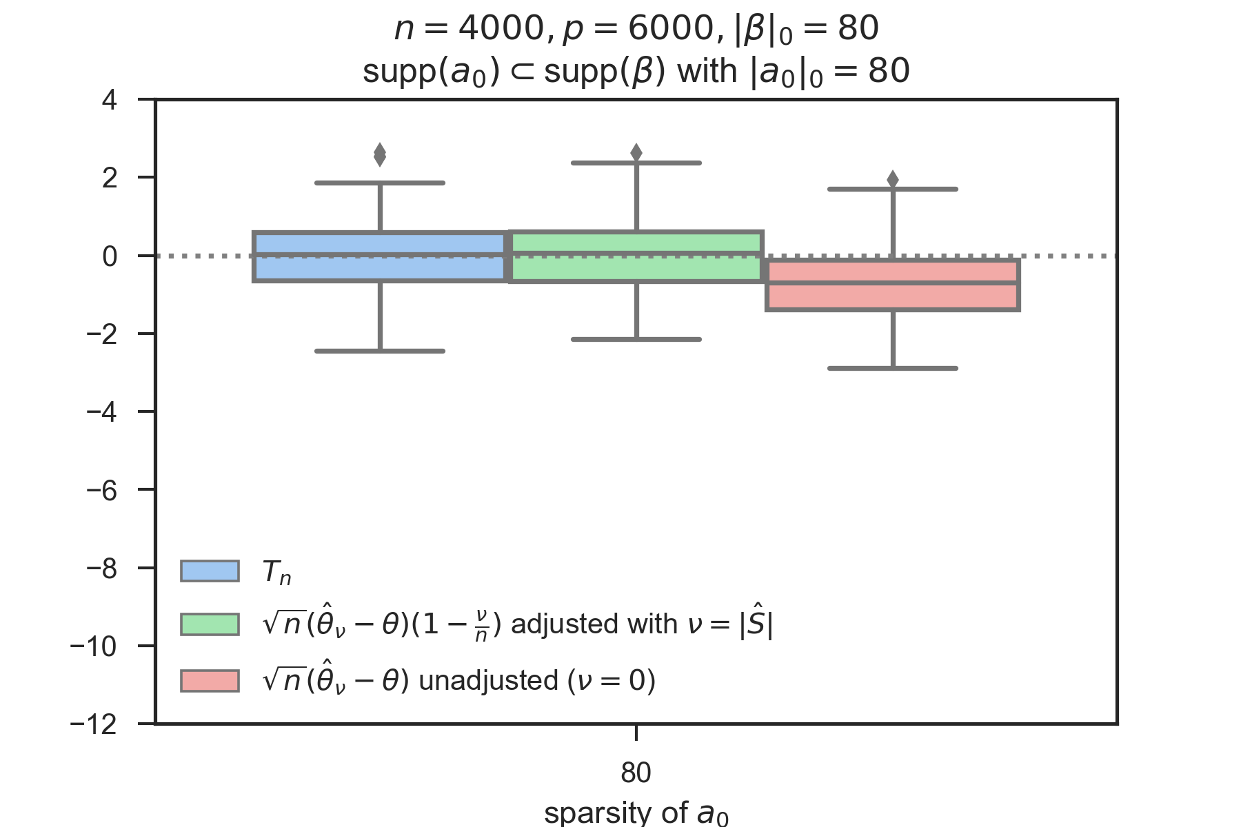
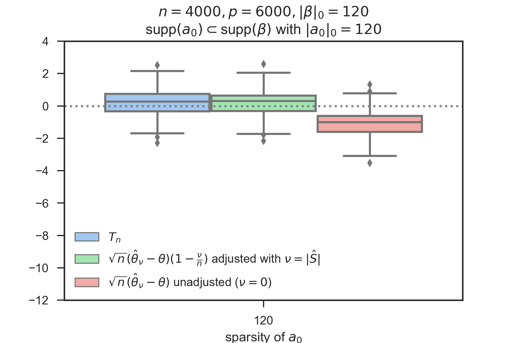
Figure 1: Distribution of $\sqrt{n}(\hat{\theta}_{\nu}-\theta)$ in the adjusted ($\nu=|{\widehat{S}}|$) and unadjusted $\nu=0$ cases. For comparison, $T_{n}$ has the t-distribution with $n$ degrees-of-freedom. Here $\boldsymbol{a}_{0}$ is proportional to $\hbox{\rm sgn}(\boldsymbol{\beta})$ normalized with $\|\boldsymbol{\Sigma}^{-1/2}\boldsymbol{a}_{0}\|_{2}=1$. Experiments were replicated 200 times. A two-sided t-test rejects that the mean of $\sqrt{n}(\hat{\theta}_{\nu}-\theta)$ is zero in the unadjusted case $(\nu=0)$ with p-value $0.0048$ for $s_{0}=20$, p-value $0.00028$ for $s_{0}=40$, p-value $7\cdot 10^{-22}$ for $s_{0}=80$ and p-value $2\cdot 10^{-31}$ for $s_{0}=120$.

Guided by Theorem 2.3, one can easily exhibit situations with correlated $\boldsymbol{\Sigma}$ and $\boldsymbol{a}_{0}$ proportional to $\boldsymbol{e}_{j}$ (a canonical basis vector), such that the unadjusted estimate leads to spurious inference: One just needs to find problem instances such that (2.14) is large. As an example, Figure 2 shows boxplots of the situation with $\boldsymbol{a}_{0}=\boldsymbol{e}_{j}/(\boldsymbol{\Sigma}^{-1})_{jj}^{1/2}$ sparsity $s_{0}=\|\boldsymbol{\beta}\|_{0}=120$, $p=6000$, $n=4000$, $\sigma=1$ and $\boldsymbol{\Sigma}$ is correlated of the form $\boldsymbol{\Sigma}^{-1}=\boldsymbol{I}_{p}+0.07(\hbox{\rm sgn}(\boldsymbol{\beta})\boldsymbol{e}_{j}^{\top}+\boldsymbol{e}_{j}\hbox{\rm sgn}(\boldsymbol{\beta})^{\top})$. In the un-adjusted case, the pivotal quantity $n^{1/2}(\hat{\theta}_{\nu=0}-\theta)$ is biased downward and would produce misleading confidence intervals with incorrect coverage. The adjustment $\nu=|{\widehat{S}}|$ exactly repairs this.

.

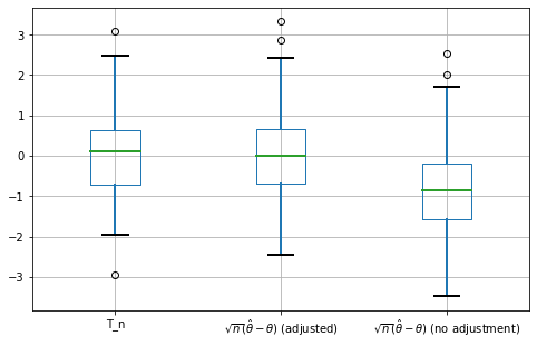
Figure 2: Boxplots of pivotal random variables $\sqrt{n}(\hat{\theta}_{n}-\theta)$ for $\nu=0$ (unadjusted) and $\nu=|{\widehat{S}}|$ (adjusted) when $\boldsymbol{a}_{0}=\boldsymbol{e}_{j}/(\boldsymbol{\Sigma}^{-1})_{jj}^{1/2}$, $s_{0}=\|\boldsymbol{\beta}\|_{0}=120$, $p=6000$, $n=4000$, $\sigma=1$ and $\boldsymbol{\Sigma}^{-1}=\boldsymbol{I}_{p}+0.07(\hbox{\rm sgn}(\boldsymbol{\beta})\boldsymbol{e}_{j}^{\top}+\boldsymbol{e}_{j}\hbox{\rm sgn}(\boldsymbol{\beta})^{\top})$. For comparison, $T_{n}$ has the t-distribution with $n$ degrees-of-freedom.

Theorem 2.3 requires sign consistency of the Lasso in (2.11). Sufficient conditions for the sign consistency of the Lasso were given in [MB06, Tro06, ZY06, Wai09]. In particular, [Wai09] gave the following sufficient conditions for (2.11) in the case of linear regression (1.1) with Gaussian design: For certain positive $\gamma$, $\delta$ and $\phi_{p}\geq 2$,

$$\big{\|}\boldsymbol{\Sigma}_{S^{c},S}\boldsymbol{\Sigma}_{S,S}^{-1}\hbox{\rm sgn}(\boldsymbol{\beta}_{S})\big{\|}_{\infty}\leq 1-\gamma,$$

$$\lambda=\gamma^{-1}\sigma\sqrt{\phi_{p}\rho(2/n)\log p},$$

$$\rho(C_{\min}\gamma^{2})^{-1}(2s_{0}/n)\log(p-s_{0})+(\phi_{p}\log p)^{-1}\log(p-s_{0})<1-\delta,$$

with $\rho=\max_{j\in S^{c}}\big{(}\boldsymbol{\Sigma}_{j,j}-\boldsymbol{\Sigma}_{j,S}\boldsymbol{\Sigma}_{S,S}^{-1}\boldsymbol{\Sigma}_{S,j}\big{)}$ and $C_{\min}=\min_{\|\boldsymbol{u}\|_{2}=1}\big{\|}\boldsymbol{\Sigma}_{S,S}^{-1/2}\boldsymbol{u}\big{\|}_{2}$, and

$$\hbox{$\min_{j\in S}$}|\beta_{j}|\geq\big{(}1+n^{-1/2}c_{n}\big{)}\lambda\max_{\|\boldsymbol{u}\|_{\infty}=1}\big{\|}\boldsymbol{\Sigma}^{-1/2}_{S,S}\boldsymbol{u}\big{\|}_{\infty}^{2}+20\big{(}\sigma^{2}(C_{\min}n)^{-1}\log s_{0}\big{)}^{1/2},$$

for some $c_{n}\to\infty$.

2.2 Unknown $\boldsymbol{\Sigma}$

In the case of unknown $\boldsymbol{u}_{0}$, one needs to estimate the ideal score vector $\boldsymbol{z}_{0}=\boldsymbol{X}\boldsymbol{u}_{0}$ as well as the variance level $\|\boldsymbol{z}_{0}\|^{2}/n$ in (1.8). In view of (1.6), we consider

$$\boldsymbol{z}=\boldsymbol{X}\boldsymbol{u},\ \boldsymbol{Q}=\boldsymbol{I}_{p}-\boldsymbol{u}\boldsymbol{a}_{0}^{\top}\ \hbox{ with $\boldsymbol{u}$ satisfying}\ \langle\boldsymbol{u},\boldsymbol{a}_{0}\rangle=1.$$ (2.16)

As $\boldsymbol{Q}^{2}=\boldsymbol{Q}$, by algebra and the definitions of $\boldsymbol{u}_{0}$ and $\boldsymbol{z}_{0}$ in (1.6) and (1.8),

$$\boldsymbol{z}=-\boldsymbol{X}\boldsymbol{Q}\boldsymbol{u}_{0}+\boldsymbol{z}_{0}=\boldsymbol{X}\boldsymbol{Q}\boldsymbol{\gamma}+\boldsymbol{z}_{0}$$ (2.17)

with $\boldsymbol{\gamma}=-\boldsymbol{Q}\boldsymbol{u}_{0}$ and ${\mathbb{E}}\big{[}(\boldsymbol{X}\boldsymbol{Q})^{\top}\boldsymbol{z}_{0}\big{]}=\boldsymbol{Q}^{\top}\boldsymbol{\Sigma}\boldsymbol{u}_{0}={\bf 0}$. Hence, (2.17) is a linear model with response vector ${\boldsymbol{z}}\in{}^{n}$, Gaussian design matrix $\boldsymbol{X}{\boldsymbol{Q}}\in{}^{n\times p}$ with $n$ independent rows, true coefficient vector $\boldsymbol{\gamma}$, and Gaussian noise $\boldsymbol{z}_{0}\sim N({\bf 0},C_{0}^{-2}\boldsymbol{I}_{n})$ independent of $\boldsymbol{X}{\boldsymbol{Q}}$, where $C_{0}=\|\boldsymbol{\Sigma}^{-1/2}\boldsymbol{a}_{0}\|_{2}$. Note that since $\boldsymbol{Q}$ is rank deficient, the linear model (2.17) is unidentifiable: For both ${\widetilde{\boldsymbol{\gamma}}}=-\boldsymbol{u}_{0}$ and $\boldsymbol{\gamma}=-\boldsymbol{Q}\boldsymbol{u}_{0}$ we have $\boldsymbol{X}\boldsymbol{Q}{\widetilde{\boldsymbol{\gamma}}}=\boldsymbol{X}\boldsymbol{Q}\boldsymbol{\gamma}$ so that both ${\widetilde{\boldsymbol{\gamma}}},\boldsymbol{\gamma}$ can be regarded as the true coefficient vector in the model (2.17). To solve this identifiability issue, we view the parameter space of (2.17) as the image of $\boldsymbol{Q}$ and the true coefficient vector as $\boldsymbol{\gamma}=-\boldsymbol{Q}\boldsymbol{u}_{0}$.

It is thus natural to estimate $\boldsymbol{z}_{0}$ in the linear model (2.17), as was already suggested previously for $\boldsymbol{a}_{0}=\boldsymbol{e}_{j}$ [ZZ14, VdGBRD14, JM18]. Given an estimator ${\widehat{\boldsymbol{\gamma}}}$ of $\boldsymbol{\gamma}$, we define the estimated score vector

$${\widehat{\boldsymbol{z}}}={\boldsymbol{z}-\boldsymbol{X}\boldsymbol{Q}{\widehat{\boldsymbol{\gamma}}}}$$ (2.18)

and the corresponding de-biased estimate

$$\hat{\theta}_{\nu,{\widehat{\boldsymbol{z}}}}=\langle\boldsymbol{a}_{0},\hat{\boldsymbol{\beta}}{}^{\text{\tiny(lasso)}}\rangle+\frac{\langle{\widehat{\boldsymbol{z}}},\boldsymbol{y}-\boldsymbol{X}\hat{\boldsymbol{\beta}}{}^{\text{\tiny(lasso)}}\rangle}{{(1-\nu/n)\langle{\widehat{\boldsymbol{z}}},\boldsymbol{z}\rangle}}.$$ (2.19)

This corresponds to (2.9) with the ideal score vector $\boldsymbol{z}_{0}$ replaced by ${\widehat{\boldsymbol{z}}}$.

The vector $\boldsymbol{u}$ in (2.16) that defines the linear model (2.17) should be picked carefully to yield small prediction error $\|\boldsymbol{z}_{0}-{\widehat{\boldsymbol{z}}}\|_{2}^{2}/n=\|\boldsymbol{X}\boldsymbol{Q}({\widehat{\boldsymbol{\gamma}}}-\boldsymbol{\gamma})\|_{2}^{2}/n$ in the linear model (2.16). As $\boldsymbol{z}_{0}=\boldsymbol{X}\boldsymbol{u}_{0}$ with a high-dimensional $\boldsymbol{u}_{0}$, it would be reasonable to expect that a sparsity condition on $\boldsymbol{u}_{0}$ would ensure proper convergence of ${\widehat{\boldsymbol{z}}}$ to $\boldsymbol{z}_{0}$. However, this requires a connection between the sparsity of $\boldsymbol{\gamma}=-\boldsymbol{Q}\boldsymbol{u}_{0}$ to that of $\boldsymbol{u}_{0}$. To this end, we pick

$$\boldsymbol{u}=\boldsymbol{e}_{j_{0}}/(a_{0})_{j_{0}}\ \hbox{with }\ j_{0}=\mathop{\rm arg\,max}_{j=1,\dots,p}\big{|}(a_{0})_{j}\big{|}.$$ (2.20)

For the above choice of $\boldsymbol{u}$,

$$\langle\boldsymbol{u},\boldsymbol{a}_{0}\rangle=1,\quad\|\boldsymbol{Q}\boldsymbol{h}\|_{0}\leq 1+\|\boldsymbol{h}\|_{0},\quad\|\boldsymbol{Q}\boldsymbol{h}\|_{1}\leq 2\|\boldsymbol{h}\|_{1},\quad\forall\ \boldsymbol{h}\in{}^{p},$$ (2.21)

so that the sparsity of $\boldsymbol{u}_{0}$ implies that of $\boldsymbol{\gamma}$. This leads to the Lasso estimator

$${{\widehat{\boldsymbol{\gamma}}}=\boldsymbol{Q}{\widehat{\boldsymbol{b}}}\ \text{ with }}\ {\widehat{\boldsymbol{b}}}=\mathop{\rm arg\,min}_{\boldsymbol{b}\in{}^{p}}\Big{\{}\|\boldsymbol{z}-\boldsymbol{X}\boldsymbol{Q}\boldsymbol{b}\|_{2}^{2}/(2n)+\widehat{\tau}A\lambda_{\text{\tiny univ}}\|\boldsymbol{Q}\boldsymbol{b}\|_{1}\Big{\}}$$ (2.22)

where $\lambda_{\text{\tiny univ}}=\sqrt{(2/n)\log p}$, $A$ is an upper bound for $\max_{j=1,\dots,p}\|\boldsymbol{X}\boldsymbol{Q}\boldsymbol{e}_{j}\|_{2}/n^{1/2}$ and $\widehat{\tau}$ is an estimate of the noise level $C_{0}^{-1}$ in the regression model (2.17). We note the delicate difference between (2.22) and the usual Lasso as the estimator and penalty are both restricted to the image of $\boldsymbol{Q}$. To the best of our knowledge, the regression model (2.17) in the direction (2.20), which plays a crucial role in our analysis, provides a new way of dealing with dense direction $\boldsymbol{a}_{0}$ in de-biasing the Lasso. We note that the natural choice ${\widetilde{\boldsymbol{u}}}=\boldsymbol{a}_{0}\|\boldsymbol{a}_{0}\|_{2}^{-2}$ satisfies $\langle\boldsymbol{a}_{0},{\widetilde{\boldsymbol{u}}}\rangle=1$, but for certain dense $\boldsymbol{a}_{0}$ the corresponding projection matrix ${\widetilde{\boldsymbol{Q}}}=\boldsymbol{I}_{p}-{\widetilde{\boldsymbol{u}}}\boldsymbol{a}_{0}^{\top}$ does not preserve sparsity as in (2.21).

For the purpose of the asymptotic normality result in Theorem 2.5 below, we will consider estimators ${\widehat{\boldsymbol{\gamma}}}$ satisfying

$$\|\boldsymbol{Q}({\widehat{\boldsymbol{\gamma}}}-\boldsymbol{\gamma})\|_{1}=O_{\mathbb{P}}(C_{0}^{-1})\min\big{\{}\|\boldsymbol{\gamma}\|_{0}\lambda_{\text{\tiny univ}},C_{0}\|\boldsymbol{\gamma}\|_{1}\big{\}},$$ (2.23)

$$\sup\big{\{}\langle{\widehat{\boldsymbol{z}}},\boldsymbol{X}\boldsymbol{Q}\boldsymbol{h}\rangle/n:\|\boldsymbol{Q}\boldsymbol{h}\|_{1}=1\big{\}}=O_{\mathbb{P}}(C_{0}^{-1}\lambda_{\text{\tiny univ}}).$$ (2.24)

Inequality (2.23) is the usual $\ell_{1}$ estimation rate when $\boldsymbol{\gamma}$ is sparse or $\boldsymbol{\gamma}$ has small $\ell_{1}$ norm. Condition (2.24) holds automatically for the Lasso estimator (2.22) when $C_{0}\widehat{\tau}=O_{{\mathbb{P}}}(1)$ as a consequence of the KKT conditions as explained in the following proposition.

Proposition 2.4.

Let $\boldsymbol{z}=\boldsymbol{X}\boldsymbol{u}$ and $\boldsymbol{Q}=\boldsymbol{I}_{p}-\boldsymbol{u}\boldsymbol{a}_{0}^{\top}$ be as in (2.16) with the $\boldsymbol{u}$ in (2.20). Assume that $\boldsymbol{\Sigma}_{j,j}\leq 1\,\forall j$, $\phi_{\min}(\boldsymbol{\Sigma})$ is bounded away from 0, and $\min\{\|\boldsymbol{Q}\boldsymbol{u}_{0}\|_{0}\log(p)/n,C_{0}\|\boldsymbol{Q}\boldsymbol{u}_{0}\|_{1}\sqrt{\log(p)/n}\}=o(1)$. Let $\boldsymbol{Q}{\widehat{\boldsymbol{\gamma}}}$ be as in (2.22) with a constant $A>2$ and $\widehat{\tau}$ satisfying one of the following conditions:

1. $\widehat{\tau}=\|\boldsymbol{z}-\boldsymbol{X}\boldsymbol{Q}{\widehat{\boldsymbol{\gamma}}}\|_{2}/n^{1/2}$ is the recursive solution of (2.22) as scaled Lasso [SZ12],

2. or $\widehat{\tau}$ is any estimator satisfying $1+o_{{\mathbb{P}}}(1)\leq C_{0}\widehat{\tau}\leq O_{{\mathbb{P}}}(1)$.

Then, the requirements (2.23)-(2.24) are satisfied.

Proposition 2.4 is proved in Appendix C. The following is our main result for unknown $\boldsymbol{\Sigma}$.

Theorem 2.5.

Assume that $\boldsymbol{\Sigma}_{jj}\leq 1$ for all $j\in[p]$ and that the spectrum of $\boldsymbol{\Sigma}$ is uniformly bounded away from 0 and $\infty$; e.g. $\max(\|\boldsymbol{\Sigma}\|_{op},\|\boldsymbol{\Sigma}^{-1}\|_{op})\leq 2$. Let $\lambda=1.01\sigma\sqrt{2\log(8p/s_{0})/n}$ for the Lasso (2.1) in the linear model (1.1). Let $\epsilon_{n}>0$ with $\epsilon_{n}=o(1)$ and ${\mathscr{B}}_{n}$ be the class of $(\boldsymbol{\beta},\boldsymbol{a}_{0})\in{}^{p\times 2}$ satisfying

$$\frac{\|\boldsymbol{\beta}\|_{0}\log p}{n}+\min\Big{\{}\frac{\|\boldsymbol{u}_{0}\|_{0}\log p}{n},\frac{C_{0}\|\boldsymbol{u}_{0}\|_{1}\sqrt{\log p}}{\sqrt{n}}\Big{\}}\leq\epsilon_{n}$$ (2.25)

and $\boldsymbol{a}_{0}\neq{\bf 0}$, where $\boldsymbol{u}_{0}$ is as in (1.6). Given $\boldsymbol{a}_{0}\neq{\bf 0}$, let $\boldsymbol{u}$ be as in (2.20), $\boldsymbol{Q}=\boldsymbol{I}_{p}-\boldsymbol{u}\boldsymbol{a}_{0}^{\top}$, $\boldsymbol{Q}{\widehat{\boldsymbol{\gamma}}}$ an estimator of $\boldsymbol{\gamma}=-\boldsymbol{Q}\boldsymbol{u}_{0}$ in the linear model (2.17) satisfying (2.23)-(2.24), ${\widehat{\boldsymbol{z}}}$ the estimated score vector in (2.18), and $\hat{\theta}_{\nu,{\widehat{\boldsymbol{z}}}}$ the de-biased estimate in (2.19). If $\nu=\|\hat{\boldsymbol{\beta}}{}^{\text{\tiny(lasso)}}\|_{0}$, then uniformly for $(\boldsymbol{\beta},\boldsymbol{a}_{0})\in{\mathscr{B}}_{n}$

$$\sqrt{nF_{\theta}}(\widehat{\theta}_{\nu=|{\widehat{S}}|,{\widehat{\boldsymbol{z}}}}-\theta) = Z_{n}+O_{\mathbb{P}}({r_{n}})$$

holds, where $Z_{n}\to^{d}N(0,1)$ and

$$r_{n}=r_{n,p}(\boldsymbol{\beta},\boldsymbol{a}_{0})=\min\Big{\{}\frac{(\|\boldsymbol{\beta}\|_{0}\wedge\|\boldsymbol{u}_{0}\|_{0})\log(p)}{\sqrt{n}},C_{0}\|\boldsymbol{u}_{0}\|_{1}\sqrt{\log p}\Big{\}}.$$ (2.26)

Consequently, for all $(\boldsymbol{\beta},\boldsymbol{a}_{0})\in{\mathscr{B}}_{n}$ satisfying $r_{n}\to 0$,

$$\sqrt{nF_{\theta}}(\widehat{\theta}_{\nu=|{\widehat{S}}|,{\widehat{\boldsymbol{z}}}}-\theta)\to^{d}N(0,1).$$

Theorem 2.5 is proved in Appendix C. The sparsity condition (2.25) is mild: it only requires that the squared prediction rate for $\boldsymbol{\beta}$ and $\boldsymbol{\gamma}$ converge to 0. Under this condition, Theorem 2.5 shows that estimation of $\theta$ is possible, for general directions $\boldsymbol{a}_{0}\neq 0$, at the rate $n^{-1/2}(1+r_{n})$ where $r_{n}$ is given by (2.26). The rate $n^{-1/2}(1+r_{n})$ is optimal as it matches the lower bound in Proposition 4.2 of [JM18] for the estimation of $\theta=\beta_{j}$ in the canonical basis directions $\boldsymbol{a}_{0}=\boldsymbol{e}_{j}$ stated in (1). Before Theorem 2.5, it was unknown whether the lower bound (1) can be attained (cf. for instance the discussion in Remark 4.3 of [JM18]). Theorem 2.5 closes this gap, extends the upper bound to general direction $\boldsymbol{a}_{0}$, and relaxes the $\ell_{1}$ bound on $\boldsymbol{\Sigma}$ imposed in [JM18].

The recent work [CCG19] proposes an alternative construction of a score vector for general direction $\boldsymbol{a}_{0}$ based on a quadratic program. This quadratic program is similar to the construction in [ZZ14, JM14a], with a modification to handle general direction $\boldsymbol{a}_{0}$, see [CCG19, equation (7), (8) and (10)]. The upper bounds in [CCG19, Corollaries 3 and 4] require $\|\boldsymbol{\beta}\|_{0}\lesssim\sqrt{n}/\log p$ in contrast with Theorem 2.5 where $\|\boldsymbol{\beta}\|_{0}\ggg\sqrt{n}$ is allowed.

Another recent line of research [BFZ18, ZB⁺18b, ZB18a] consider the construction of confidence intervals for $\boldsymbol{a}_{0}^{\top}\boldsymbol{\beta}$ for general directions $\boldsymbol{a}_{0}$ without sparsity assumption on $\boldsymbol{\beta}$. These works consider the setting where $\boldsymbol{\beta}$ is arbitrary but bounded in the sense that $\|\boldsymbol{\Sigma}^{1/2}\boldsymbol{\beta}\|_{2}^{2}\leq C$ for some constant $C\asymp\sigma^{2}$ independent of $n,p$. In this setting, $\|\boldsymbol{\beta}\|_{0}\log(p)/n\to 0$ is violated and consistent estimation of $\boldsymbol{\beta}$ or $\boldsymbol{Q}_{0}\boldsymbol{\beta}$ is not possible. Assuming $\|\boldsymbol{\Sigma}^{1/2}\boldsymbol{\beta}\|_{2}^{2}\leq C$ instead of a sparsity assumption on $\boldsymbol{\beta}$ leads to different minimax rates: The rate in [BFZ18, Corollary 5] does not depend on $\|\boldsymbol{\beta}\|_{0}$ but depends implicitly on $\|\boldsymbol{\Sigma}^{1/2}\boldsymbol{\beta}\|_{2}$ instead; hence the rate in Theorem 2.5 and (1) is not directly comparable to theirs. On a higher level, this line of research is fundamentally different than the present work: [BFZ18, ZB⁺18b, ZB18a] leverage the assumption that the nuisance part of the signal, $\boldsymbol{X}\boldsymbol{Q}_{0}\boldsymbol{\beta}$, is bounded with componentwise variance of the same order as that of the noise, without attempting to estimate the nuisance part of the signal. In contrast, Theorem 2.5 attemps to estimate the nuisance parameter and the nuisance part of the signal $\boldsymbol{X}\boldsymbol{Q}_{0}\boldsymbol{\beta}$ is allowed to have arbitrarily large componentwise variance.

Next, we prove that the de-biased estimator in Theorem 2.5 for unknown $\boldsymbol{\Sigma}$, and the ideal $\widehat{\theta}_{\nu}$ in (2.2) for known $\boldsymbol{\Sigma}$ as well, would not achieve the same rate without the degrees-of-freedom adjustment. Compared with Theorem 2.3, Theorem 2.6 below is somewhat less explicit but the sign consistency of the Lasso is no longer required.

Theorem 2.6.

Let $\boldsymbol{\Sigma}$, $\epsilon_{n}$, ${\mathscr{B}}_{n}$, $r_{n}$, ${\widehat{\boldsymbol{z}}}$ and $\hat{\theta}_{\nu,{\widehat{\boldsymbol{z}}}}$ be as in Theorem 2.5. Let $s_{0}$ and $s_{\Omega}$ be positive integers satisfying $s_{0}\log(p)/n\leq\epsilon_{n}$, $s_{\Omega}\leq s_{0}$ and

$$n^{-1}s_{0}s_{\Omega}^{1/2}\sqrt{\log(8p/s_{0})}\ggg 1+s_{\Omega}\log(p)/n^{1/2}.$$ (2.27)

If $\nu=0$, which means no degrees-of-freedom adjustment in (2.19), then there exist $(\boldsymbol{\beta},\boldsymbol{a}_{0})\in{\mathscr{B}}_{n}$ such that $\|\boldsymbol{\beta}\|_{0}=s_{0}$, $\|\boldsymbol{u}_{0}\|_{0}=\|\boldsymbol{\Sigma}^{-1}\boldsymbol{a}_{0}\|_{0}=s_{\Omega}$, and $\sqrt{nF_{\theta}}(\widehat{\theta}_{\nu,{\widehat{\boldsymbol{z}}}}-\theta)/(1+r_{n})$ is stochastically unbounded. Moreover, the above statement also holds when $\hat{\theta}_{\nu,{\widehat{\boldsymbol{z}}}}$ is replaced by $\widehat{\theta}_{\nu}$ in (2.2).

Theorem 2.6 is proved in Appendix C. As an example, if $s_{\Omega}=\epsilon_{n}\sqrt{n}/\log(p)$ and $s_{0}\geq\epsilon_{n}^{-1}n^{3/4}$ for some $\epsilon_{n}\to 0$, then

• (2.27) holds so that, without adjustment, $\sqrt{nF_{\theta}}(\widehat{\theta}_{\nu=0,{\widehat{\boldsymbol{z}}}}-\theta)$ is unbounded by Theorem 2.6 for some $(\boldsymbol{\beta},\boldsymbol{a}_{0})\in{\mathscr{B}}_{n}$ with $\|\boldsymbol{\beta}\|_{0}=s_{0}$ and $\|\boldsymbol{u}_{0}\|_{0}=s_{\Omega}$.

• $r_{n}\to 0$ hence $\sqrt{nF_{\theta}}(\widehat{\theta}_{\nu=|{\widehat{S}}|,{\widehat{\boldsymbol{z}}}}-\theta)\to^{d}N(0,1)$ by Theorem 2.5 and the de-biased estimate adjusted with $\nu=\|\hat{\boldsymbol{\beta}}{}^{\text{\tiny(lasso)}}\|_{0}$ is efficient for all $(\boldsymbol{\beta},\boldsymbol{a}_{0})\in{\mathscr{B}}_{n}$ with $\|\boldsymbol{\beta}\|_{0}\leq s_{0},\|\boldsymbol{u}_{0}\|_{0}\leq s_{\Omega}$.

2.3 Unknown $\boldsymbol{\Sigma}$ and canonical basis directions $\boldsymbol{a}_{0}=\boldsymbol{e}_{j}$

For convenience we provide here the notation and corollary of Theorem 2.5 in the case of canonical basis vector $\boldsymbol{a}_{0}=\boldsymbol{e}_{j}$ for some $j\in\{1,\dots,p\}$. We denote $(\boldsymbol{u}_{0},\boldsymbol{z}_{0},{\widehat{\boldsymbol{z}}})$ by $(\boldsymbol{u}_{j},\boldsymbol{z}_{j},{\widehat{\boldsymbol{z}}}_{j})$ and write the linear model (2.17) as

$$\boldsymbol{X}\boldsymbol{e}_{j}=\boldsymbol{X}^{(-j)}~{}\boldsymbol{\gamma}^{(j)}+\boldsymbol{z}_{j}$$ (2.28)

where $\boldsymbol{X}^{(-j)}\in{}^{n\times(p-1)}$ is the matrix $\boldsymbol{X}$ with $j$-th column removed, $\boldsymbol{\gamma}^{(j)}\in{}^{p-1}$. The corresponding vector $\boldsymbol{u}_{0}$ is $\boldsymbol{u}_{j}=(\boldsymbol{\Sigma}^{-1})_{jj}^{-1}\boldsymbol{\Sigma}^{-1}\boldsymbol{e}_{j}$ which is related to $\boldsymbol{\gamma}^{(j)}$ by $(\boldsymbol{u}_{j})_{j}=1$ and $(\boldsymbol{u}_{j})_{(-j)}=-\boldsymbol{\gamma}^{(j)}$. The ideal score vector $\boldsymbol{z}_{0}$ becomes $\boldsymbol{z}_{j}=(\boldsymbol{\Sigma}^{-1})_{jj}^{-1}\boldsymbol{X}\boldsymbol{\Sigma}^{-1}\boldsymbol{e}_{j}$ and has iid $N(0,(\boldsymbol{\Sigma}^{-1})_{jj}^{-1})$ entries independent of $\boldsymbol{X}^{(-j)}$. For a given estimator ${\widehat{\boldsymbol{\gamma}}}^{(j)}$ of $\boldsymbol{\gamma}^{(j)}$, the score vector (2.18) is then ${\widehat{\boldsymbol{z}}}_{j}=\boldsymbol{X}\boldsymbol{e}_{j}-\boldsymbol{X}^{(-j)}{\widehat{\boldsymbol{\gamma}}}^{(j)}$ and the de-biased estimate (2.19) reduces to

$$\hat{\beta}_{j}^{\text{\tiny(de-biased)}}=(\hat{\boldsymbol{\beta}}{}^{\text{\tiny(lasso)}})_{j}+\frac{\langle{\widehat{\boldsymbol{z}}}_{j},\boldsymbol{y}-\boldsymbol{X}\hat{\boldsymbol{\beta}}{}^{\text{\tiny(lasso)}}\rangle}{(1-\nu/n)\langle{\widehat{\boldsymbol{z}}}_{j},\boldsymbol{X}\boldsymbol{e}_{j}\rangle}.$$ (2.29)

which corresponds to the proposal in [ZZ14] modified with the degrees-of-freedom adjustment $(1-\nu/n)$. For $\boldsymbol{a}_{0}=\boldsymbol{e}_{j}$, the Lasso estimator (2.22) becomes

$${\widehat{\boldsymbol{\gamma}}}^{(j)}=\mathop{\rm arg\,min}_{\boldsymbol{\gamma}\in{}^{p-1}}\left\{\frac{1}{2n}\|\boldsymbol{X}\boldsymbol{e}_{j}-\boldsymbol{X}^{(-j)}\boldsymbol{\gamma}\|_{2}^{2}+\hat{\tau}_{j}{\overline{\lambda}}\|\boldsymbol{\gamma}\|_{1}\right\}.$$ (2.30)

with recursive solution $\hat{\tau}_{j}=\|\boldsymbol{X}\boldsymbol{e}_{j}-\boldsymbol{X}^{(-j)}\boldsymbol{\gamma}\|_{2}/n^{1/2}$ in the scaled Lasso [SZ12] or any estimate $\hat{\tau}_{j}$ satisfying $1+o_{{\mathbb{P}}}(1)\leq(\boldsymbol{\Sigma}^{-1})_{j,j}\hat{\tau}_{j}^{2}\leq O_{{\mathbb{P}}}(1)$. As the choice of $\boldsymbol{u}$ in (2.20) for $\boldsymbol{a}_{0}=\boldsymbol{e}_{j}$ is $\boldsymbol{u}=\boldsymbol{e}_{j}$, the proof of Theorem 2.5 can be modified to allow ${\overline{\lambda}}=A\lambda_{\text{\tiny univ}}$ with $A>1$, since in this case ${\mathbb{E}}\|\boldsymbol{X}\boldsymbol{Q}\boldsymbol{a}_{0}\|_{2}^{2}/n$ is bounded from the above by 1.

Corollary 2.7.

Assume that $\boldsymbol{\Sigma}_{jj}\leq 1$ for all $j\in[p]$ and that the spectrum of $\boldsymbol{\Sigma}$ is uniformly bounded away from 0 and $\infty$; e.g. $\max(\|\boldsymbol{\Sigma}\|_{op},\|\boldsymbol{\Sigma}^{-1}\|_{op})\leq 2$. Let $\lambda=1.01\sigma\sqrt{2\log(8p/s_{0})/n}$ for the Lasso (2.1). Consider the Scaled Lasso in (2.30) with ${\overline{\lambda}}=1.01\sqrt{2\log(p)/n}$, the corresponding score vector ${\widehat{\boldsymbol{z}}}_{j}$ and de-biased estimate $\widehat{\beta}_{j}^{\text{\tiny(de-biased)}}$ in (2.29) with $\nu=\|\hat{\boldsymbol{\beta}}{}^{\text{\tiny(lasso)}}\|_{0}$. Then for any $j$,

$$\frac{(\|\boldsymbol{\beta}\|_{0}\vee\|\boldsymbol{\Sigma}^{-1}\boldsymbol{e}_{j}\|_{0})\log(p)}{n}\to 0\text{ and }\frac{(\|\boldsymbol{\beta}\|_{0}\wedge\|\boldsymbol{\Sigma}^{-1}\boldsymbol{e}_{j}\|_{0})\log(p)}{\sqrt{n}}\to 0$$ (2.31)

implies $\sqrt{n}(\boldsymbol{\Sigma}^{-1})_{jj}^{-1/2}(\widehat{\beta}_{j}^{\text{\tiny(de-biased)}}-\beta_{j})\to^{d}N(0,\sigma^{2})$.

Remark 2.1.

The tuning parameters of the present section are chosen as $\lambda=1.01\sigma\sqrt{2\log(8p/s_{0})/n}$ for simplicity of the presentation. As the results of the present section are consequences of Theorem 3.1 in the next section, more general tuning parameters of the form (3.4) are also allowed and the resulting constants in the theorems would then depend on certain constants $\eta_{2}\in(0,1),\eta_{3}>0$.

3 Theoretical results for known $\boldsymbol{\Sigma}$

In this section, we prove that the degrees-of-freedom adjusted LDPE in (2.2) indeed removes the bias of the Lasso for the estimation of a general linear functional $\theta=\langle\boldsymbol{a}_{0},\boldsymbol{\beta}\rangle$ when $(s_{0}/n)\log(p/s_{0})$ is sufficiently small and a sparse Riesz condition (SRC) [ZH08] holds on the population covariance matrix $\boldsymbol{\Sigma}$ of the Gaussian design.

The SRC is closely related to the restricted isometry property (RIP) [CT05, CT07]. While the RIP is specialized for nearly uncorrelated design variables in the context of compressed sensing, the SRC is more suitable in analysis of data from observational studies or experiments with higher correlation in the design. For example, the SRC allows an upper sparse eigenvalue greater than 2. For $p\times p$ positive semi-definite matrices $\boldsymbol{M}$, integers $1\leq m\leq p$ and a support set $B\subset\{1,\ldots,p\}$, define a lower sparse eigenvalue as

$$\phi_{\min}(m,B;\boldsymbol{M})=\min_{A\subset[p]:|A\setminus B|=m}\phi_{\min}\Big{(}\boldsymbol{M}_{A,A}\Big{)}$$ (3.1)

and an upper sparse eigenvalue as

$$\phi_{\max}(m,B;\boldsymbol{M})=\max_{A\subset[p]:|A\setminus B|=m}\phi_{\max}\Big{(}\boldsymbol{M}_{A,A}\Big{)},$$ (3.2)

where $\phi_{\min}(\boldsymbol{M})$ and $\phi_{\max}(\boldsymbol{M})$ are respectively the smallest and largest eigenvalues of symmetric matrix $\boldsymbol{M}$. Define similarly the sparse condition number by

$$\phi_{\rm cond}(m;B,\boldsymbol{M})=\max_{A\subset[p]:|A\setminus{B}|\leq(1\vee m)}\big{\{}\phi_{\max}(\boldsymbol{M}_{A,A})/\phi_{\min}(\boldsymbol{M}_{A,A})\big{\}}.$$ (3.3)

Recall that $S$ is the support of $\boldsymbol{\beta}$ and $s_{0}=|S|$. For a precise statement of the sample size requirement for our main results, we will assume the following.

Assumption 3.1.

Assume that $\boldsymbol{\Sigma}$ is invertible with diagonal elements at most 1, i.e., $\max_{j=1,...,p}\Sigma_{jj}\leq 1$. Consider positive integers $\{m,n,p,k\}$ and positive constants $\{\rho_{*},\eta_{2},\eta_{3},\epsilon_{1},\epsilon_{2},\epsilon_{3},\epsilon_{4}\}$ with $\eta_{2},\eta_{3}\in(0,1)$. Set the tuning parameter of the Lasso by

$$\lambda=\eta_{2}^{-1}(1+\eta_{3})\sigma\lambda_{0},\qquad\text{where}\qquad\lambda_{0}=\sqrt{(2/n)\log(8p/k)}.$$ (3.4)

Define $\{\tau_{*},\tau^{*}\}$ by $\tau_{*}=(1-\epsilon_{1}-\epsilon_{2})^{2}$, $\tau^{*}=(1+\epsilon_{1}+\epsilon_{2})^{2}$ and assume that

$${s_{0}}+k<\frac{(1-\eta_{2})^{2}2m}{(1+\eta_{2})^{2}\big{\{}(\tau^{*}/\tau_{*})\phi_{\rm cond}(m+k;S,\boldsymbol{\Sigma})-1\big{\}}}$$ (3.5)

and $\rho_{*}\leq\phi_{\min}(m+k,S;\boldsymbol{\Sigma})$ hold. Assume that $\lambda_{0}\sqrt{s_{*}}\leq 1$ where $s_{*}=s_{0}+m+k$, as well as

$$2(m+k)+s_{0}+1\leq(n-1)\wedge(p+1),$$ (3.6)

$$\epsilon_{1}+\epsilon_{2}<1,\quad\epsilon_{3}+\epsilon_{4}=\epsilon_{2}^{2}/8,$$ (3.7)

$$s_{0}+m+k+1\leq\min(p+1,\epsilon_{1}^{2}n/2),\quad\log\binom{p-s_{0}}{m+k}\leq\epsilon_{3}n.$$ (3.8)

Typical values of $k,m$ and $\{\rho_{*},\eta_{2},\eta_{3},\epsilon_{1},\epsilon_{2},\epsilon_{3},\epsilon_{4}\}$ are given after Corollary 3.2 below. As will become clear in the proofs in Appendix A, the integer $k$ above is an upper bound on the cardinality of the set

$$B=\{j\in[p]:|{\boldsymbol{\varepsilon}}^{\top}\boldsymbol{x}_{j}|/n\geq\eta_{2}\lambda\},$$ (3.9)

i.e., the set of covariates that correlate highly with the noise. If $k=1$ then $\lambda=\eta_{2}^{-1}(1+\eta_{3})\sigma\sqrt{(2/n)\log(8p)}$ and the set $B$ is empty with high probability. The integer $m$ is, with high probability, an upper bound on the cardinality of the set $\operatorname{supp}(\hat{\boldsymbol{\beta}}{}^{\text{\tiny(lasso)}})\setminus(S\cup B)$. In other words, the support of $\hat{\boldsymbol{\beta}}{}^{\text{\tiny(lasso)}}$ contains at most $m$ variables that are neither in the true support $S$ nor in the set $B$ of highly correlated covariates. These statements are made rigorous in Sections A.1 and A.2. Results of the form $|{\widehat{S}}|=O_{\mathbb{P}}(s_{0})$ have appeared before for the Lasso, see for instances [ZH08, Theorem 1], [BRT09, Eq. (7.9)], [ZZ12, Corollary 2 (ii)] and [BCW14, Theorem 3]. Among these existing bounds, the theory derived in the present paper is closest to [ZZ12, Corollary 2 (ii)] where a bound of the form $|{\widehat{S}}|=O_{\mathbb{P}}(s_{0})$ is derived under a condition on the upper sparse eigenvalue (3.2) after a prediction error bound under a weak restricted eigenvalue condition. They depart from other existing bounds of the form $|{\widehat{S}}|=O_{\mathbb{P}}(s_{0})$ in several ways. The bounds in [ZH08, Theorem 1] requires the tuning parameter to be set as a function of the sparse eigenvalues of $\boldsymbol{X}^{\top}\boldsymbol{X}/n$. The bound from [BRT09] involves $\phi_{\max}(\boldsymbol{X}^{\top}\boldsymbol{X}/n)$ which is unbounded if $p/n\to+\infty$ for Gaussian designs. The bound [BCW14, Theorem 3] tackles tuning parameters larger than $\sigma\sqrt{2\log(p)/n}$ but does not provide guarantees for smaller tuning parameters of order $\sigma\sqrt{2\log(8p/k)/n}$. The theory developed for the present paper in Appendix A improves upon these aforementioned references: The theory only requires bounds on sparse condition number (cf. the SRC condition (3.5)), the tuning parameters need not depend on the sparse eigenvalues, and small tuning parameters of order $\sigma\sqrt{2\log(8p/k)/n}$ are allowed. Furthermore, the theory in Appendix A clearly separates the roles of $s_{0},k$ and $m$: $k$ is an upper bound on the cardinality of the set (3.9) of covariates highly correlated with the noise, $m$ is an upper bound on $\operatorname{supp}(\hat{\boldsymbol{\beta}}{}^{\text{\tiny(lasso)}})\setminus(S\cup B)$, and consequently $\|\hat{\boldsymbol{\beta}}{}^{\text{\tiny(lasso)}}\|_{0}\leq s_{0}+k+m$.

Stochastically bounded $O_{\mathbb{P}}(\cdot)$ notation

In the following results, we consider an asymptotic regime with growing $\{s_{0},m,k,n,p\}$ such that

$$p/k\to+\infty,\qquad s_{*}\lambda_{0}^{2}\to 0$$ (3.10)

where $s_{*}=s_{0}+m+k$. This means that we consider a sequence of regression problems (1.1) indexed by $n$ and $\{s_{0},m,k,p\}$ are functions of $n$ such that (3.10) holds and Assumption 3.1 is satisfied for all $n$ with constants $\{\rho_{*},\eta_{2},\eta_{3},\epsilon_{1},\epsilon_{2},\epsilon_{3},\epsilon_{4}\}$ independent of $n$. For a deterministic sequence $a_{n}$, we write $W_{n}=O_{\mathbb{P}}(a_{n})$ if the sequence of random variables $(W_{n})$ is such that for any arbitrarily small $\gamma>0$, there exists constants $K,N$ depending on $\gamma$ and $\{\rho_{*},\eta_{2},\eta_{3},\epsilon_{1},\epsilon_{2},\epsilon_{3},\epsilon_{4}\}$ such that for all $n\geq N$, ${\mathbb{P}}(W_{n}>K)\leq\gamma.$ We also write $W_{n}=o_{\mathbb{P}}(1)$ if $W_{n}=O_{\mathbb{P}}(a_{n})$ for some $a_{n}\to 0$. Under the above Assumption 3.1, our main result is the following.

Theorem 3.1.

Let (3.10) and Assumption 3.1 be fulfilled. Let $F_{\theta}=1/(\sigma C_{0})^{2}$ be the Fisher information as in (1.7), and $T_{n}=\sqrt{nF_{\theta}}\langle\boldsymbol{z}_{0},{\boldsymbol{\varepsilon}}\rangle/\|\boldsymbol{z}_{0}\|_{2}^{2}$ so that $T_{n}$ has the $t$-distribution with $n$ degrees of freedom. For any random degrees-of-freedom adjustment $\nu\in[0,n]$ we have

$$\sqrt{nF_{\theta}}(1-\nu/n)(\widehat{\theta}_{\nu}-\theta)=T_{n}+\sqrt{F_{\theta}/n}\left\langle\boldsymbol{a}_{0},\hat{\boldsymbol{\beta}}{}^{\text{\tiny(lasso)}}-\boldsymbol{\beta}\right\rangle\left(|{\widehat{S}}|-\nu\right)+O_{\mathbb{P}}\left(\lambda_{0}\sqrt{s_{*}}\right).$$

If the condition number $\phi_{\rm cond}(p;\emptyset,\boldsymbol{\Sigma})=\|\boldsymbol{\Sigma}\|_{op}\|\boldsymbol{\Sigma}^{-1}\|_{op}$ of the population covariance matrix $\boldsymbol{\Sigma}$ is bounded, then $O_{\mathbb{P}}\left(\lambda_{0}\sqrt{s_{*}}\right)$ above can be replaced by $O_{\mathbb{P}}\left(\lambda_{0}\sqrt{s_{0}+k}\right)$ [by $O_{\mathbb{P}}\left(\lambda_{0}\sqrt{s_{0}}\right)$ when the penalty is chosen with $k\lesssim s_{0}$ in (3.4)].

The result is proved in Section 8.4. If $\lambda_{0}\sqrt{s_{*}}\to 0$ and $k/p\to 0$, the above result implies that $\sqrt{nF_{\theta}}(1-\nu/n)(\widehat{\theta}_{\nu}-\theta)$ is within $o_{\mathbb{P}}(1)$ of $T_{n}$ of the $t$-distribution with $n$ degrees of freedom if and only if

$$\sqrt{F_{\theta}/n}\left\langle\boldsymbol{a}_{0},\hat{\boldsymbol{\beta}}{}^{\text{\tiny(lasso)}}-\boldsymbol{\beta}\right\rangle\left(|{\widehat{S}}|-\nu\right)=o_{\mathbb{P}}(1).$$ (3.11)

The left hand side of (3.11) is negligible either because the modified de-biasing scheme (2.2) is correctly adjusted with $\nu=|{\widehat{S}}|$ (or $\nu\approx|{\widehat{S}}|$) to account for the degrees of freedom of the initial estimator $\hat{\boldsymbol{\beta}}{}^{\text{\tiny(lasso)}}$, or because the estimation error of the initial estimator $\langle\boldsymbol{a}_{0},\hat{\boldsymbol{\beta}}{}^{\text{\tiny(lasso)}}-\boldsymbol{\beta}\rangle$ is significantly small.

The choice of degrees-of-freedom adjustment $\nu=|{\widehat{S}}|$ ensures that the quantity (3.11) is always equal to 0. This leads to the following corollary.

Corollary 3.2.

Let (3.10) and Assumption 3.1 be fulfilled. With the notation from Theorem 3.1, if $\nu=|{\widehat{S}}|$ then

$$\sqrt{nF_{\theta}}\left(1-|{\widehat{S}}|/n\right)\left(\widehat{\theta}_{\nu=|{\widehat{S}}|}-\theta\right)=T_{n}+O_{\mathbb{P}}\left(\lambda_{0}\sqrt{s_{*}}\right).$$ (3.12)

Hence if $\lambda_{0}\sqrt{s_{*}}\to 0$ and $k/p\to 0$, the de-biasing scheme (2.2) correctly adjusted with $\nu=|{\widehat{S}}|$ enjoys asymptotic efficiency. To highlight this fact and give an example of typical values for $m,k$ and $\{\rho_{*},\eta_{2},\eta_{3},\epsilon_{1},\epsilon_{2},\epsilon_{3},\epsilon_{4}\}$ in Assumption 3.1, let us explain how Corollary 3.2 implies (2.3) of Theorem 2.1. Set $\eta_{2}^{-1}=\sqrt{1.01}$, $\eta_{3}=\sqrt{1.01}-1$ and $k=s_{0}$, so that the tuning parameter (3.4) is equal to $\lambda$ defined in Theorem 2.1. Set also $\epsilon_{1}=\epsilon_{2}=1/4$ so that $\tau_{*}=1/4,\tau^{*}=9/4$. Under the assumptions of Theorem 2.1, the spectrum of $\boldsymbol{\Sigma}$ is bounded away from 0 and $\infty$ (e.g. a subset of $[1/2,2]$) and the sparse condition number appearing in (3.5) is bounded (e.g. at most 4 respectively). Next, set $m=Cs_{0}$ for some large enough absolute constant $C>0$ chosen so that (3.5) holds; this gives $s_{*}=s_{0}+m+k=(C+2)s_{0}$. The conditions in Assumption 3.1 are satisfied thanks to $\lambda_{0}\sqrt{s_{*}}\to 0$ and $k/p\to 0$. By Lemma 8.1 we get $|{\widehat{S}}|=O_{\mathbb{P}}(s_{0})$. Then (2.3) is a direct consequence of (3.12).

By Theorem 3.1, the unadjusted de-biasing scheme (1.8) enjoys asymptotic efficiency for all fixed $\boldsymbol{a}_{0}$ and $\boldsymbol{\beta}$ with $\|\boldsymbol{\beta}\|_{0}\leq s_{0}$ if and only if (3.11) holds with $\nu=0$, i.e., if

$$\sqrt{F_{\theta}/n}\left\langle\boldsymbol{a}_{0},\hat{\boldsymbol{\beta}}{}^{\text{\tiny(lasso)}}-\boldsymbol{\beta}\right\rangle|{\widehat{S}}|=o_{\mathbb{P}}(1).$$ (3.13)

By the Cauchy-Schwarz inequality, $|\langle\boldsymbol{a}_{0},\hat{\boldsymbol{\beta}}{}^{\text{\tiny(lasso)}}-\boldsymbol{\beta}\rangle|\leq C_{0}\|\boldsymbol{\Sigma}^{1/2}(\hat{\boldsymbol{\beta}}{}^{\text{\tiny(lasso)}}-\boldsymbol{\beta})\|_{2}$. Under Assumption 3.1 or other typical conditions on the restricted eigenvalues of $\boldsymbol{\Sigma}$ and the sample size, the population risk $\|\boldsymbol{\Sigma}^{1/2}(\hat{\boldsymbol{\beta}}{}^{\text{\tiny(lasso)}}-\boldsymbol{\beta})\|_{2}$ is of order $O_{\mathbb{P}}(\sigma\lambda_{0}\sqrt{s_{*}})$ which grants (3.13) if $\lambda_{0}\sqrt{s_{*}}s_{*}/\sqrt{n}\to 0$. This is the content of the following corollary which is formally proved in Section 8.5.

Corollary 3.3 (Unadjusted LDPE).

Let (3.10) and Assumption 3.1 be fulfilled. With the notation from Theorem 3.1, if $\nu=0$ then

$$\sqrt{nF_{\theta}}(\widehat{\theta}_{\nu=0}-\theta)=T_{n}+O_{\mathbb{P}}\left(\lambda_{0}\sqrt{s_{*}}\left(1+\frac{s_{*}}{\sqrt{n}}\right)\right).$$ (3.14)

If $\lambda_{0}^{2}(s_{*})^{3}/n\to 0$ then the right hand side of (3.14) converges in probability to $T_{n}$. In this asymptotic regime, the degrees-of-freedom adjustment is not necessary and the unadjusted (1.8) enjoys asymptotic efficiency. Note that although the adjustment $\nu=|{\widehat{S}}|$ that leads to the efficiency of $\widehat{\theta}_{\nu}$ in Corollary 3.2 is not necessary in this particular asymptotic regime, such adjustment does not harm either. Since the practitioner cannot establish whether the asymptotic regime $\lambda_{0}^{2}(s_{*})^{3}/n\to 0$ actually occurs because $s_{0}$ and $s_{*}$ are unknown, it is still recommended to use the adjustment $\nu=|{\widehat{S}}|$ as in Corollary 3.2 to ensure efficiency for the whole range of sparsity.

An outcome of Theorem 2.3 is that the unadjusted de-biasing scheme (1.8) cannot be efficient in the regime (2.15). By Theorem 2.3 and the discussion surrounding (2.15) on the one hand, and Corollary 3.3 and the discussion of the previous paragraph on the other hand, we have established the following phase transition:

• If $\lambda_{0}^{2}(s_{*})^{3}/n\lll 1$, the unadjusted de-biasing scheme (1.8) is efficient for every $\boldsymbol{a}_{0}$, by Corollary 3.3.

• If $\lambda_{0}^{2}s_{0}^{3}/n\ggg 1$, the unadjusted de-biasing scheme (1.8) cannot be efficient for certain specific $\boldsymbol{a}_{0}$.

In other words, there is a phase transition at $s_{*}\asymp n^{2/3}$ (up to a logarithmic factor) where degrees-of-freedom adjustment becomes necessary to achieve asymptotic efficiency for all preconceived directions $\boldsymbol{a}_{0}$. Condition $s_{*}\lll n^{2/3}$ is a weaker requirement than the assumption $s_{*}\lll\sqrt{n}$ commonly made in the literature on de-biasing.

4 De-biasing without degrees of freedom adjustment under additional assumptions on $\boldsymbol{\Sigma}$

The left hand side of (3.13) quantifies the remaining bias of the unadjusted de-biasing scheme (1.8). Under an additional assumption on $\boldsymbol{\Sigma}$, namely a bound on $\|\boldsymbol{\Sigma}^{-1}\boldsymbol{a}_{0}\|_{1}$, the initial bias of the Lasso $\langle\boldsymbol{a}_{0},\hat{\boldsymbol{\beta}}{}^{\text{\tiny(lasso)}}-\boldsymbol{\beta}\rangle$ is small enough to grant asymptotic efficiency to the unadjusted de-biasing scheme (1.8). The following theorem makes this precise.

Theorem 4.1.

Let (3.10) and Assumption 3.1 be fulfilled. Suppose

$$\|\boldsymbol{\Sigma}^{-1}\boldsymbol{a}_{0}\|_{1}/\|\boldsymbol{\Sigma}^{-1/2}\boldsymbol{a}_{0}\|_{2}\leq K_{0,n,p}=K_{1,n,p}\sqrt{n/s_{*}}$$ (4.1)

for some quantities $K_{0,n,p}$ and $K_{1,n,p}$. Then, $\sqrt{F_{\theta}}|\langle\boldsymbol{a}_{0},\hat{\boldsymbol{\beta}}{}^{\text{\tiny(lasso)}}-\boldsymbol{\beta}\rangle|=O_{\mathbb{P}}(\lambda_{0}K_{0,n,p})$ and

$$\sqrt{nF_{\theta}}(\widehat{\theta}_{\nu=0}-\theta)=T_{n}+O_{{\mathbb{P}}}\big{(}(1+K_{1,n,p})\lambda_{0}\sqrt{s_{*}}+s_{*}/n\big{)}.$$

This implies that $\sqrt{nF_{\theta}}(\widehat{\theta}_{\nu=0}-\theta)=T_{n}+o_{\mathbb{P}}(1)$ when $K_{1,n,p}=O(1)$.

The proof is given in Appendix B. In other words, the unadjusted de-biasing scheme (1.8) is efficient and degrees-of-freedom adjustment is not needed for efficiency if the $\ell_{1}$ norm of $\boldsymbol{\Sigma}^{-1}\boldsymbol{a}_{0}$ is bounded from above as in

$$\|\boldsymbol{\Sigma}^{-1}\boldsymbol{a}_{0}\|_{1}/\|\boldsymbol{\Sigma}^{-1/2}\boldsymbol{a}_{0}\|_{2}=O(\sqrt{n/s_{*}})$$

with $s_{*}/p\to 0$ and $(s_{*}/n)\log(p/s_{*})\to 0$. This improves by a logarithmic factor the condition $\|\boldsymbol{\Sigma}^{-1}\boldsymbol{a}_{0}\|_{1}/\|\boldsymbol{\Sigma}^{-1/2}\boldsymbol{a}_{0}\|_{2}=O(1)$ required for efficiency in [JM18].

The above result explains why the necessity of degrees-of-freedom adjustment did not appear in previous analysis such as [JM18]; $\sqrt{F_{\theta}}|\langle\boldsymbol{a}_{0},\hat{\boldsymbol{\beta}}{}^{\text{\tiny(lasso)}}-\boldsymbol{\beta}\rangle|=O_{\mathbb{P}}(\lambda_{0})$ when $K_{0,n,p}=O(1)$ in (4.1), and the unadjusted de-biasing scheme (1.8) is efficient when $K_{1,n,p}=O(1)$ in (4.1). However, by Theorem 2.3 and the discussion surrounding (2.15), there exist certain $\boldsymbol{a}_{0}$ with large $\|\boldsymbol{\Sigma}^{-1}\boldsymbol{a}_{0}\|_{1}/\|\boldsymbol{\Sigma}^{-1/2}\boldsymbol{a}_{0}\|_{2}$ such that the unadjusted de-biasing scheme cannot be efficient. For such $\boldsymbol{a}_{0}$, degrees-of-freedom adjustments are necessary to achieve efficiency.

5 An $\ell_{\infty}$ error bound for the Lasso

The idea of the previous section can be applied to $\boldsymbol{a}_{0}=\boldsymbol{e}_{j}$ simultaneously for all vectors $\boldsymbol{e}_{j}$ of the canonical basis $(\boldsymbol{e}_{1},...,\boldsymbol{e}_{p})$. This yields the following $\ell_{\infty}$ bound on the error of the Lasso.

Theorem 5.1.

Let Assumption 3.1 be fulfilled, and further assume that $\log p<n$. Then the Lasso satisfies simultaneously for all $j=1,...,p$

$$\left|\widehat{\beta}{}^{\text{\tiny(lasso)}}_{j}-\beta_{j}\right|\leq\frac{M_{5}^{2}\|\boldsymbol{\Sigma}^{-1}\boldsymbol{e}_{j}\|_{1}\lambda+{\sigma\|\boldsymbol{\Sigma}^{-1/2}\boldsymbol{e}_{j}\|_{2}}\sqrt{\log p/n}\left(2M_{5}+3\bar{M}\lambda_{0}\sqrt{s_{*}}\right)}{1-s_{*}/n}$$ (5.1)

on an event $\Omega_{\ell_{\infty}}$ such that ${\mathbb{P}}(\Omega_{\ell_{\infty}}^{c})\to 0$ when (3.10) holds, where $s_{*}=s_{0}+m+k$, $M_{5}=1/(1-\eta_{3})$ and $\bar{M}$ is a constant that depends on $\{\rho_{*},\eta_{2},\eta_{3},\epsilon_{1},\epsilon_{2},\epsilon_{3},\epsilon_{4}\}$ only. Consequently, since $\|\boldsymbol{\Sigma}^{-1/2}\boldsymbol{e}_{j}\|_{2}\leq\|\boldsymbol{\Sigma}^{-1}\boldsymbol{e}_{j}\|_{1}$, on the same event we have

$$\|\hat{\boldsymbol{\beta}}{}^{\text{\tiny(lasso)}}-\boldsymbol{\beta}\|_{\infty}\leq\rho(\boldsymbol{\Sigma})\left(\frac{M_{5}^{2}+2M_{5}+4\bar{M}\lambda_{0}\sqrt{s_{*}}}{1-s_{*}/n}\right)\max\left(\lambda,\sigma\sqrt{\frac{\log p}{n}}\right)$$

where $\rho(\boldsymbol{\Sigma})=\max_{j=1,...,p}\|\boldsymbol{\Sigma}^{-1}\boldsymbol{e}_{j}\|_{1}$.

The proof is given in Appendix B. The above result asserts that if the $\ell_{1}$-norms of the columns of $\boldsymbol{\Sigma}^{-1}$ are bounded from above by some constant $\rho(\boldsymbol{\Sigma})>0$ then

$$\|\hat{\boldsymbol{\beta}}{}^{\text{\tiny(lasso)}}-\boldsymbol{\beta}\|_{\infty}\leq C(\boldsymbol{\Sigma})\max(\lambda,\sigma\sqrt{\log(p)/n})$$

holds with overwhelming probability for some constant $C(\boldsymbol{\Sigma})\lesssim\rho(\boldsymbol{\Sigma})$.

Although some $\ell_{\infty}$ bounds for the lasso have appeared previously in the literature, we are not aware of previous results comparable to Theorem 5.1 for $s_{0}\ggg\sqrt{n}$. The result of [Lou08] and [BC13, Theorem 2(2)] requires incoherence conditions on the design, i.e., that non-diagonal elements of $\boldsymbol{X}^{\top}\boldsymbol{X}/n$ are smaller than $1/s_{0}$ up to a constant. This assumption is strong and cannot be satisfied in the regime $s_{0}\ggg\sqrt{n}$, even for the favorable $\boldsymbol{\Sigma}=\boldsymbol{I}_{p}$: for $\boldsymbol{\Sigma}=\boldsymbol{I}_{p}$ the standard deviation of the $i,j$-th entry is ${\mathbb{E}}[(\boldsymbol{X}^{\top}\boldsymbol{X}/n)_{ij}^{2}]^{1/2}=1/\sqrt{n}$. In a random design setting comparable to ours, Section 4.4 of [vdG16] explains that $\|{\hat{\boldsymbol{\beta}}{}^{\text{\tiny(lasso)}}}-\boldsymbol{\beta}\|_{\infty}\lesssim\max_{j}\|\boldsymbol{\Sigma}^{-1}\boldsymbol{e}_{j}\|_{1}\sigma\sqrt{\log(p)/n}(1+\|{\hat{\boldsymbol{\beta}}{}^{\text{\tiny(lasso)}}}-\boldsymbol{\beta}\|_{1}/\sigma)$. This bound is only comparable to our $\ell_{\infty}$ bound in the regime $\|{\hat{\boldsymbol{\beta}}{}^{\text{\tiny(lasso)}}}-\boldsymbol{\beta}\|_{1}=O_{P}(1)$, i.e., in the regime $s_{0}\lesssim\sqrt{n}$ (up to logarithmic factors) since $\|{\hat{\boldsymbol{\beta}}{}^{\text{\tiny(lasso)}}}-\boldsymbol{\beta}\|_{1}\approx\lambda s_{0}\approx\sigma s_{0}\sqrt{\log(p)/n}$. Again this result is not applicable (or substantially worse than Theorem 5.1) in the more challenging regime $s_{0}\ggg\sqrt{n}$ of interest here.

6 Regularity and asymptotic efficiency

Theorem 2.1(i) shows that the test statistic $\sqrt{nF_{\theta}}(1-|{\widehat{S}}|/n)(\hat{\theta}_{\nu}-\boldsymbol{a}_{0}^{\top}\boldsymbol{\beta})$, properly adjusted with $\nu=|{\widehat{S}}|$, converges in distribution to $N(0,1)$, where $F_{\theta}=1/\{\sigma^{2}C_{0}^{2}\}$ and $C_{0}=\|\boldsymbol{\Sigma}^{-1/2}\boldsymbol{a}_{0}\|$. This holds under any sequence of distributions $\{\mathbb{P}_{0}^{n}\}_{n\geq 1}$ defined by $\|\boldsymbol{\beta}\|=s_{0}$, $s_{0}\log(p/s_{0})/n\to 0$, $\max(\|\boldsymbol{\Sigma}\|_{op},\|\boldsymbol{\Sigma}^{-1}\|_{op})\leq K$ for some constant $K$ independent of $n,p$, and

$$\boldsymbol{X}\text{ has iid rows }N({\bf 0},\boldsymbol{\Sigma}),\qquad\boldsymbol{y}|\boldsymbol{X}\sim N(\boldsymbol{X}\boldsymbol{\beta},\sigma^{2}\boldsymbol{I}_{n}).$$

Here, we denote the unknown parameter $\boldsymbol{a}_{0}^{\top}\boldsymbol{\beta}$ by $\theta(\boldsymbol{P}^{n}_{0})$ to avoid confusion with the probability measures defined in the next paragraph. By Slutsky’s theorem, since $|{\widehat{S}}|/n$ converges to 0 in probability by Theorem 2.1(i), we have

$$\mathcal{L}\left(\sqrt{nF_{\theta}}(\hat{\theta}_{\nu}-\theta({\mathbb{P}}_{0}^{n}))~{};~{}\mathbb{P}_{0}^{n}\right)\to N(0,1).$$ (6.1)

Given $\boldsymbol{a}_{0}\in{}^{p}$, a positive-definite matrix $\boldsymbol{\Sigma}\in{}^{p\times p}$ and $\mathcal{B}_{n}\subset{}^{p}$ as a parameter space, let $F_{\theta}$ be as in (1.7),

$$\mathcal{U}_{n}\subseteq\Big{\{}\boldsymbol{u}\subset{}^{p}:\boldsymbol{u}^{\top}\boldsymbol{a}_{0}=1,\,\boldsymbol{\beta}+t\boldsymbol{u}/\sqrt{nF_{\theta}}\in\mathcal{B}_{n}\,\forall t\in[0,t_{\boldsymbol{u}}],\,t_{\boldsymbol{u}}\to\infty\Big{\}}$$

as a collection of directions of univariate sub-models $\{\boldsymbol{\beta}+t\boldsymbol{u}/\sqrt{nF_{\theta}}:0\leq t\leq t_{\boldsymbol{u}}\}$. For $t>0$ and $\boldsymbol{u}\in\mathcal{U}_{n}$ let ${\mathbb{P}}_{t,\boldsymbol{u}}^{n}$ be probabilities under which

$$\boldsymbol{y}|\boldsymbol{X}\sim N\left(\boldsymbol{X}(\boldsymbol{\beta}+t\boldsymbol{u}/\sqrt{nF_{\theta}}),\sigma^{2}\boldsymbol{I}_{n}\right)$$ (6.2)

(for either deterministic or possibly non-Gaussian random $\boldsymbol{X}$) and

$$\theta({\mathbb{P}}^{n}_{t,\boldsymbol{u}})=\left\langle\boldsymbol{a}_{0},\boldsymbol{\beta}+t\boldsymbol{u}/\sqrt{nF_{\theta}}\right\rangle=\left\langle\boldsymbol{a}_{0},\boldsymbol{\beta}\right\rangle+t/\sqrt{nF_{\theta}}.$$

That is, under $\mathbb{P}_{t,\boldsymbol{u}}^{n}$ the vector $\boldsymbol{\beta}$ is perturbed with the additive term $t\boldsymbol{u}/\sqrt{nF_{\theta}}$, resulting a perturbation of the parameter of interest with $t/\sqrt{nF_{\theta}}$. In the above framework, an estimator $\widetilde{\theta}$ is regular (in the directions $\boldsymbol{u}\in\mathcal{U}_{n}$) if

$$\mathcal{L}\left(\sqrt{nF_{\theta}}(\widetilde{\theta}-\theta({\mathbb{P}}_{t,\boldsymbol{u}}^{n}))~{};~{}{\mathbb{P}}_{t,\boldsymbol{u}}^{n}\right)\to G$$ (6.3)

for all fixed $t>0$ and $\boldsymbol{u}\in\mathcal{U}_{n}$ and some distribution $G$ not depending on $t$ and $\boldsymbol{u}$. That is, the limiting distribution is stable under the small perturbation as defined above.

Our first task is to show that $\widehat{\theta}_{\nu}$ is regular in all directions with the same limiting distribution as in (6.1), i.e. (6.3) holds with $\mathcal{U}_{n}={}^{p}$ and $G\sim N(0,1)$. For $t=0$, (6.1) is implied by Theorem 2.1(i). However Theorem 2.1(i) does not directly imply (6.3) for $t\neq 0$ because ${\boldsymbol{u}\in\mathcal{U}_{n}}$, as well as the unknown regression vector $\boldsymbol{\beta}+{t\boldsymbol{u}/\sqrt{nF_{\theta}}}$ under ${\mathbb{P}}_{{t,\boldsymbol{u}}}^{n}$, may not be sparse. The following device due to Le Cam shows that (6.3) still holds with the perturbation $t{\boldsymbol{u}}/\sqrt{nF_{\theta}}$ for any fixed $t\neq 0$ independent of $n,p$.

The likelihood-ratio $L_{n}$ between $\mathbb{P}^{n}_{t,{\boldsymbol{u}}}$ and $\mathbb{P}^{n}_{0}$ is given by

$$\log L_{n} = \{-\|\boldsymbol{y}-\boldsymbol{X}(\boldsymbol{\beta}+t{\boldsymbol{u}/\sqrt{nF_{\theta}}})\|^{2}+\|\boldsymbol{y}-\boldsymbol{X}\boldsymbol{\beta}\|^{2}\}/(2\sigma^{2}).$$

$$= -t^{2}C_{0}^{2}\|{\boldsymbol{X}\boldsymbol{u}}\|^{2}/(2n)-\langle{\boldsymbol{\varepsilon}},{\boldsymbol{X}\boldsymbol{u}}\rangle tC_{0}/(\sigma\sqrt{n}).$$

Under $\mathbb{P}^{n}_{0}$, the random variable $\sqrt{nF_{\theta}}(\widehat{\theta}_{\nu}-\theta({\mathbb{P}}_{0}^{n}))$ can be written as $\langle{\boldsymbol{\varepsilon}},\boldsymbol{z}_{0}\rangle C_{0}/(\sqrt{n}\sigma)+o_{\mathbb{P}}(1)$ so that the vector $(\sqrt{nF_{\theta}}(\widehat{\theta}_{\nu}-\theta({\mathbb{P}}_{0}^{n})),\log L_{n})^{\top}$ converges in distribution under $\mathbb{P}^{n}_{0}$ to a bivariate normal vector with mean $(0,-t^{2}C_{0}^{2}\langle\boldsymbol{u},\boldsymbol{\Sigma}\boldsymbol{u}\rangle/2)^{\top}$ and covariance

$$\Big{(}\begin{smallmatrix}1&tC_{0}^{2}\langle\boldsymbol{u}_{0},\boldsymbol{\Sigma}\boldsymbol{u}\rangle\\ tC_{0}^{2}\langle\boldsymbol{u}_{0},\boldsymbol{\Sigma}\boldsymbol{u}\rangle\quad&t^{2}C_{0}^{2}\langle\boldsymbol{u},\boldsymbol{\Sigma}\boldsymbol{u}\rangle\end{smallmatrix}\Big{)}=\Big{(}\begin{smallmatrix}1&t\\ t&\quad t^{2}C_{0}^{2}\langle\boldsymbol{u},\boldsymbol{\Sigma}\boldsymbol{u}\rangle\end{smallmatrix}\Big{)},$$

where the equality is due to $\boldsymbol{u}_{0}=C_{0}^{-2}\boldsymbol{\Sigma}^{-1}\boldsymbol{a}_{0}$ and $\langle\boldsymbol{a}_{0},\boldsymbol{u}\rangle=1$. It directly follows by Le Cam’s third lemma (see, for instance, [VdV00, Example 6.7]) that $\sqrt{nF_{\theta}}(\widehat{\theta}_{\nu}-\theta({\mathbb{P}}_{0}^{n}))$ converges to $N(t,1)$ under $\{\mathbb{P}^{n}_{t,{\boldsymbol{u}}}\}_{n\geq 1}$ and that (6.3) holds. For more details, see also [VdV00, Section 7.5] about situations where the log-likelihood ratio converges to normal distributions of the form $N(-a^{2}/2,a^{2})$.

Hence, properly adjusted with $\nu=|{\widehat{S}}|$, the estimator $\hat{\theta}_{\nu}$ is regular and asymptotic normality still holds if the sparse coefficient vector $\boldsymbol{\beta}$ is replaced by $\boldsymbol{\beta}+t{\boldsymbol{u}}/\sqrt{nF_{\theta}}$ for constant $t\in{\real}$, even if the perturbation ${\boldsymbol{u}}$ is non-sparse. By the Le Cam-Hayek convolution theorem (see, for instance, [VdV00, Theorem 8.8]), the asymptotic variance of $\sqrt{n}(\hat{\theta}_{\nu}-\theta)$ must be at least $1/F_{\theta}$ and our estimator $\widehat{\theta}_{\nu}$ is efficient, i.e., it achieves the smallest possible asymptotic variance among regular estimators.

Note that the above reasoning does not inherently rely on the Gaussian design assumption. As soon as the second moment of the row of $\boldsymbol{X}$ exists, $\|{\boldsymbol{X}\boldsymbol{u}}\|^{2}/(n\langle\boldsymbol{u},\boldsymbol{\Sigma}\boldsymbol{u}\rangle)\to 1$ and $\langle\boldsymbol{X}\boldsymbol{u},\boldsymbol{X}\boldsymbol{u}_{0}\rangle/(n\langle\boldsymbol{u}_{0},\boldsymbol{\Sigma}\boldsymbol{u}\rangle)\to 1$ almost surely by the law of large numbers. If additionally ${\boldsymbol{\varepsilon}}\sim N({\bf 0},\sigma^{2}\boldsymbol{I}_{n})$ and $\boldsymbol{X}$ is such that $\sqrt{nF_{\theta}}(\hat{\theta}_{\nu}-\boldsymbol{a}_{0}^{\top}\boldsymbol{\beta})=\langle{\boldsymbol{\varepsilon}},\boldsymbol{z}_{0}\rangle C_{0}/(\sigma\sqrt{n})+o_{\mathbb{P}^{n}_{0}}(1)$ for sparse $\boldsymbol{\beta}$, the argument of the previous paragraph is applicable and $\hat{\theta}_{\nu}$ is regular in the sense of (6.3). For instance, if $\boldsymbol{a}_{0}$ is a canonical basis vector, equation $\sqrt{nF_{\theta}}(\hat{\theta}_{\nu=0}-\boldsymbol{a}_{0}^{\top}\boldsymbol{\beta})=\langle{\boldsymbol{\varepsilon}},\boldsymbol{z}_{0}\rangle C_{0}/(\sigma\sqrt{n})+o_{\mathbb{P}^{n}_{0}}(1)$ can be obtained for sub-gaussian design and $s_{0}\lll\sqrt{n}$ using an $\ell_{1}/\ell_{\infty}$ duality inequality, cf. [ZZ14, VdGBRD14, JM14a]. In such asymptotic regime, the argument of the previous paragraph shows that $\hat{\theta}_{\nu=0}$ is stable for non-sparse perturbations of the form $t{\boldsymbol{u}}/\sqrt{nF_{\theta}}$.

We formally state the above analysis and existing lower bounds,

Proposition 6.1.

Let $\mathcal{V}_{n}$ be the linear span of $\mathcal{U}_{n}$ as a tangent space. Suppose

$${\mathbb{P}}_{0}^{n}\Big{\{}\Big{|}\|\boldsymbol{X}\boldsymbol{u}\|_{2}^{2}/(n\boldsymbol{u}^{\top}\boldsymbol{\Sigma}\boldsymbol{u})-1\Big{|}>\epsilon\Big{\}}=o(1),\qquad{\boldsymbol{u}\in\mathcal{U}_{n},}$$

and dim$(\mathcal{V}_{n})=O(1)$. Let $\boldsymbol{u}_{0}$ be as in (1.6) and $\tau=\tau(\mathcal{V}_{n})={\widetilde{\boldsymbol{u}}}_{0}^{\top}\boldsymbol{\Sigma}{\widetilde{\boldsymbol{u}}}_{0}/F_{\theta}$ with

$${\widetilde{\boldsymbol{u}}}_{0}=\mathop{\rm arg\,min}\Big{\{}\boldsymbol{u}^{\top}\boldsymbol{\Sigma}\boldsymbol{u}:\boldsymbol{u}\in\mathcal{V}_{n},\langle\boldsymbol{a}_{0},\boldsymbol{u}\rangle=1\Big{\}}.$$

(i) Let $\widetilde{\theta}$ be a regular estimator in the sense of (6.3) with a limiting distribution $G$. Let $\xi\sim G$. Then, (a) $\hbox{\rm Var}(\xi)\geq 1/\tau$; (b) If $\hbox{\rm Var}(\xi)=1/\tau$, then $\xi\sim N(0,1/\tau)$; (c) If ${{\widetilde{\boldsymbol{u}}}_{0}}=a_{1}\boldsymbol{u}_{1}+a_{2}\boldsymbol{u}_{2}$ for two $\boldsymbol{u}_{1},\boldsymbol{u}_{2}\in\mathcal{U}_{n}$ and $\{a\boldsymbol{u}_{1}+(1-a)\boldsymbol{u}_{2}:0\leq a\leq 1\}\subseteq\mathcal{U}_{n}$, then $\xi=\xi_{1}+\xi_{2}$ where $\xi_{1}\sim N(0,1/\tau)$ and $\xi_{2}$ is independent of $\xi_{1}$.
(ii) If $\boldsymbol{u}_{0}\in\mathcal{V}_{n}$, then ${\widetilde{\boldsymbol{u}}}_{0}=\boldsymbol{u}_{0}$ and $\tau=\tau(\mathcal{V}_{n})=1$.
(iii) If (6.1) holds, then $\widehat{\theta}_{\nu}$ is regular and locally asymptotically efficient in the sense of (6.3) with $\mathcal{B}_{n}=\mathcal{U}_{n}={}^{p}$.

The above statement is somewhat more general than the usual version as we wish to accommodate general parameter space $\mathcal{B}_{n}$, cf. [VdV00, Theorem 8.8] for $\mathcal{U}_{n}=\{\boldsymbol{u}\in\mathcal{V}_{n}:\langle\boldsymbol{a}_{0},\boldsymbol{u}\rangle=1\}$ and [Sch86] and [Zha05, Theorem 6.1] for general $\mathcal{U}_{n}$. We note that the condition on ${{\widetilde{\boldsymbol{u}}}_{0}}$ in Proposition 6.1(i)(c), known as the convolution theorem, is equivalent to the convexity of $\mathcal{U}_{n}$ and ${{\widetilde{\boldsymbol{u}}}_{0}}\in\mathcal{V}_{n}$. The minimum Fisher information is sometimes defined as $\min\{{\sigma^{-2}}\boldsymbol{u}^{\top}\boldsymbol{\Sigma}\boldsymbol{u}:\langle\boldsymbol{a}_{0},\boldsymbol{u}\rangle=1,\boldsymbol{u}\in\mathcal{U}_{n}\}$. However, when this minimum over $\mathcal{U}_{n}$ is strictly larger than the minimum over its linear span $\mathcal{V}_{n}$, the larger minimum information is not attainable by estimators regular with respect to $\mathcal{U}_{n}$ in virtue of (i)(a) above.

In Proposition 6.1, the parameter $\tau=\tau(\mathcal{V}_{n})$ can be viewed as the relative efficiency for the tangent space $\mathcal{V}_{n}$ generated by the collection $\mathcal{U}_{n}$ of directions of univariate sub-models. As the minimization for ${\widetilde{\boldsymbol{u}}}_{0}$ is taken over no greater a space compared with (1.6), $\tau\geq 1$ always holds. When the parameter space $\mathcal{B}_{n}$ is strictly smaller than ^p or the regularity (stability of the limiting distribution) is required only for deviations from the true $\boldsymbol{\beta}$ in a small collection of directions, $\tau>1$ may materialize and an estimator regular and efficient relative to $\mathcal{U}_{n}$ would become super-efficient in the full model with $\mathcal{B}_{n}=\mathcal{V}_{n}={}^{p}$. According to Le Cam’s local asymptotic minimax theorem, in the full model, such a super-efficient estimator would perform strictly worse than a regular efficient estimator when the true $\boldsymbol{\beta}$ is slightly perturbed in a certain direction.

The super-efficiency was observed in [vdG17] where an estimator, also based on the de-biased lasso, achieves asymptotic variance strictly smaller than $1/F_{\theta}$. The construction of [vdG17, Theorem 2.1] goes as follows: Consider a sequence $\lambda_{n}^{\sharp}$ and a sequence of sub-regions $\mathcal{B}_{n}\subset{}^{p}$ of the parameter space such that the Lasso satisfies uniformly over all $\boldsymbol{\beta}\in\mathcal{B}_{n}$ both

$$\|\boldsymbol{\Sigma}^{1/2}(\hat{\boldsymbol{\beta}}{}^{\text{\tiny(lasso)}}-\boldsymbol{\beta})\|_{2}=o_{\mathbb{P}}(1),\qquad\sqrt{n}\lambda^{\sharp}_{n}\|\hat{\boldsymbol{\beta}}{}^{\text{\tiny(lasso)}}-\boldsymbol{\beta}\|_{1}=o_{\mathbb{P}}(1).$$

Then [vdG17] constructs an asymptotically normal estimator of the first component $\beta_{1}$ of $\boldsymbol{\beta}$. However, this estimator depends on a fixed sub-region $\mathcal{B}_{n}$ that achieves a particular $\ell_{1}$ convergence rate given by $\lambda^{\sharp}_{n}$, and the estimator would need to be changed to satisfy asymptotic normality on a superset of $\mathcal{B}_{n}$. Hence this construction is a super-efficiency phenomenon: it is possible to achieve a strictly smaller variance than the Fisher information lower bound with the $F_{\theta}$ in (1.7) as the estimators are only required to perform well on a specific parameter space $\mathcal{B}_{n}$. Additionally, the estimator from [vdG17] cannot be regular on perturbations of the form $\boldsymbol{\beta}+t\boldsymbol{u}_{0}/\sqrt{nF_{\theta}}$ for non-sparse $\boldsymbol{u}_{0}$, otherwise that estimator would not be able to achieve an asymptotic variance smaller than $1/F_{\theta}$ according to Proposition 6.1.

7 Necessity of the degrees-of-freedom adjustment in a more general setting

This section extends Theorem 2.3 to subgaussian designs. It shows that the degrees-of-freedom adjustment is necessary when the Lasso is sign-consistent.

Theorem 7.1.

Let $S$ be a support of size $s_{0}=o(n)$ and assume that $\boldsymbol{X}_{S}\boldsymbol{\Sigma}_{S,S}^{-1/2}$ has iid entries from a mean-zero, variance one and subgaussian distribution. Assume that $(\boldsymbol{\beta},\boldsymbol{a}_{0})$ follows a prior independent of $(\boldsymbol{X},{\boldsymbol{\varepsilon}})$ with $\operatorname{supp}(\boldsymbol{\beta})=S$, $\boldsymbol{\beta}$ has iid random signs on $S$ and fixed amplitudes $\{|\beta_{j}|,j\in S\}$, and set $\boldsymbol{a}_{0}=\boldsymbol{\Sigma}\hbox{\rm sgn}(\boldsymbol{\beta})_{S}/\sqrt{s_{0}}$. Then on the selection event $\{{\widehat{S}}=S,\hbox{\rm sgn}(\hat{\boldsymbol{\beta}}{}^{\text{\tiny(lasso)}})=\hbox{\rm sgn}(\boldsymbol{\beta})\}$, the de-biased estimate $\widehat{\theta}_{\nu}$ in (2.8) with adjustment $\nu$ satisfies

$$\sqrt{n}(1-\nu/n)(\widehat{\theta}_{\nu}-\theta)-\sqrt{n}(1-\nu/n)\langle\boldsymbol{a}_{0},(\boldsymbol{X}_{S}^{\top}\boldsymbol{X}_{S})^{-1}\boldsymbol{X}_{S}^{\top}{\boldsymbol{\varepsilon}}\rangle$$

$$= -(s_{0}-\nu)\left(\lambda\sqrt{n}\boldsymbol{a}_{0}^{\top}(\boldsymbol{X}_{S}^{\top}\boldsymbol{X}_{S})^{-1}\hbox{\rm sgn}(\boldsymbol{\beta})_{S}\right)$$

$$+O_{\mathbb{P}}\left(\lambda\sqrt{s_{0}\log s_{0}}+\phi_{\rm cond}(\boldsymbol{\Sigma}_{S,S})^{1/2}\lambda{\sqrt{s_{0}}}\right).$$

Furthermore, $\lambda\sqrt{n}\boldsymbol{a}_{0}^{\top}\left[(\boldsymbol{X}_{S}^{\top}\boldsymbol{X}_{S})^{-1}\right]\hbox{\rm sgn}(\boldsymbol{\beta})_{S}=\lambda\sqrt{s_{0}/n}(1-o_{P}(1))$ when $\phi_{\rm cond}(\boldsymbol{\Sigma}_{S,S})\leq C$ for some constant $C>0$ independent of $n,p,s_{0}$. Consequently, if $\nu=0$ and $s_{0}^{3/2}\geq n$, the right-hand side above is unbounded.

The proof is given in Appendix I. In conclusion, for designs with subgaussian independent entries and under sign-consistency for the Lasso, the unadjusted $\widehat{\theta}_{\nu}$ with $\nu=0$ is not asymptotically normal as soon as $s_{0}\ggg n^{2/3}$, similarly to the Gaussian design case and the conclusion of Theorem 2.3.

8 Outline of the proof

8.1 The interpolation path

Throughout the sequel, let $\boldsymbol{h}{}^{\text{\tiny(lasso)}}=\hat{\boldsymbol{\beta}}{}^{\text{\tiny(lasso)}}-\boldsymbol{\beta}$. It follows from the definition of $\widehat{\theta}_{\nu}$ in (2.2) that

$$(1-\nu/n)\big{(}\widehat{\theta}_{\nu}-\theta\big{)}=\frac{\big{\langle}\boldsymbol{z}_{0},{\boldsymbol{\varepsilon}}\big{\rangle}}{\|\boldsymbol{z}_{0}\|_{2}^{2}}-(\nu/n)\big{\langle}\boldsymbol{a}_{0},\boldsymbol{h}{}^{\text{\tiny(lasso)}}\big{\rangle}-\frac{\big{\langle}\boldsymbol{z}_{0},\boldsymbol{X}\boldsymbol{Q}_{0}\boldsymbol{h}{}^{\text{\tiny(lasso)}}\big{\rangle}}{\|\boldsymbol{z}_{0}\|_{2}^{2}}$$

with $\boldsymbol{z}_{0}=\boldsymbol{X}\boldsymbol{u}_{0}$ and $\boldsymbol{Q}_{0}=\boldsymbol{I}_{p\times p}-\boldsymbol{u}_{0}\boldsymbol{a}_{0}^{\top}$, where $\boldsymbol{u}_{0}=\boldsymbol{\Sigma}^{-1}\boldsymbol{a}_{0}/\langle\boldsymbol{a}_{0},\boldsymbol{\Sigma}^{-1}\boldsymbol{a}_{0}\rangle$.

In the above expression, $\boldsymbol{z}_{0}$ is independent of $(\boldsymbol{X}\boldsymbol{Q}_{0},{\boldsymbol{\varepsilon}})$ but not of $\hat{\boldsymbol{\beta}}{}^{\text{\tiny(lasso)}}$. If $\boldsymbol{z}_{0}$ were independent of $\boldsymbol{X}\boldsymbol{Q}_{0}\boldsymbol{h}{}^{\text{\tiny(lasso)}}$, we would have

$${\mathscr{L}}\Big{(}\big{\langle}\boldsymbol{z}_{0},\boldsymbol{X}\boldsymbol{Q}_{0}\boldsymbol{h}{}^{\text{\tiny(lasso)}}\big{\rangle}\Big{|}\boldsymbol{X}\boldsymbol{Q}_{0}\boldsymbol{h}{}^{\text{\tiny(lasso)}}\Big{)} \sim N\Big{(}0,C_{0}^{-2}\|\boldsymbol{X}\boldsymbol{Q}_{0}\boldsymbol{h}{}^{\text{\tiny(lasso)}}\|_{2}^{2}\Big{)}$$

$$=O_{\mathbb{P}}(1/C_{0})\|\boldsymbol{X}\boldsymbol{Q}_{0}\boldsymbol{h}{}^{\text{\tiny(lasso)}}\|_{2},$$ (8.1)

where ${\mathscr{L}}(\xi|\zeta)$ denotes the conditional distribution of $\xi$ given $\zeta$ and $C_{0}=\|\boldsymbol{\Sigma}^{-1/2}\boldsymbol{a}_{0}\|_{2}$. Our idea is to decouple $\boldsymbol{z}_{0}$ and $\hat{\boldsymbol{\beta}}{}^{\text{\tiny(lasso)}}$ by replacing $\boldsymbol{z}_{0}$ with an almost independent copy of itself in the definition of $\hat{\boldsymbol{\beta}}{}^{\text{\tiny(lasso)}}$.

We proceed as follows. Let $\boldsymbol{g}\sim N({\bf 0},{\mathbb{E}}[\boldsymbol{z}_{0}\boldsymbol{z}_{0}^{\top}])$ be a random vector independent of $({\boldsymbol{\varepsilon}},\boldsymbol{z}_{0},\boldsymbol{X})$ such that $\boldsymbol{g}$ and $\boldsymbol{z}_{0}$ have the same distribution. Next, define the random vector

$${\widetilde{\boldsymbol{z}}}_{0}=\boldsymbol{P}_{\boldsymbol{\varepsilon}}\boldsymbol{z}_{0}+\boldsymbol{P}^{\perp}_{\boldsymbol{\varepsilon}}\boldsymbol{g},\quad\text{ where }\ \boldsymbol{P}_{\boldsymbol{\varepsilon}}=\|{\boldsymbol{\varepsilon}}\|^{-2}{\boldsymbol{\varepsilon}}{\boldsymbol{\varepsilon}}^{\top}\ \text{ and }\ \boldsymbol{P}_{\boldsymbol{\varepsilon}}^{\perp}=\boldsymbol{I}_{n}-\boldsymbol{P}_{\boldsymbol{\varepsilon}}.$$

Conditionally on ${\boldsymbol{\varepsilon}}$, the random vectors $\boldsymbol{z}_{0}$ and $\tilde{\boldsymbol{z}}_{0}$ are identically distributed, so that ${\widetilde{\boldsymbol{z}}}_{0}$ is independent of $(\boldsymbol{X}\boldsymbol{Q}_{0},{\boldsymbol{\varepsilon}})$.

Next, let ${\widetilde{\boldsymbol{X}}}=\boldsymbol{X}\boldsymbol{Q}_{0}+{\widetilde{\boldsymbol{z}}}_{0}\boldsymbol{a}_{0}^{\top}$ and let $\tilde{\boldsymbol{\beta}}{}^{\text{\tiny(lasso)}}$ be the Lasso solution with $(\boldsymbol{X},\boldsymbol{y})$ replaced by $({\widetilde{\boldsymbol{X}}},{\widetilde{\boldsymbol{X}}}\boldsymbol{\beta}+{\boldsymbol{\varepsilon}})$. Conditionally on ${\boldsymbol{\varepsilon}}$, the random vector $\boldsymbol{P}_{\boldsymbol{\varepsilon}}^{\perp}\boldsymbol{z}_{0}$ is normally distributed and independent of $\boldsymbol{X}\boldsymbol{Q}_{0}{\widetilde{\boldsymbol{h}}}{}^{\text{\tiny(lasso)}}$ by construction, so that

$$\left|\big{\langle}\boldsymbol{z}_{0},\boldsymbol{X}\boldsymbol{Q}_{0}{\widetilde{\boldsymbol{h}}}{}^{\text{\tiny(lasso)}}\big{\rangle}\right| \leq \left|\big{\langle}\boldsymbol{P}_{\boldsymbol{\varepsilon}}^{\perp}\boldsymbol{z}_{0},\boldsymbol{X}\boldsymbol{Q}_{0}{\widetilde{\boldsymbol{h}}}{}^{\text{\tiny(lasso)}}\big{\rangle}\right|+\|\boldsymbol{P}_{\boldsymbol{\varepsilon}}\boldsymbol{z}_{0}\|\;\;\|\boldsymbol{P}_{\boldsymbol{\varepsilon}}\boldsymbol{X}\boldsymbol{Q}_{0}{\widetilde{\boldsymbol{h}}}{}^{\text{\tiny(lasso)}}\|,$$

$$\leq O_{\mathbb{P}}(1/C_{0})\left(\|\boldsymbol{P}_{\boldsymbol{\varepsilon}}^{\perp}\boldsymbol{X}\boldsymbol{Q}_{0}{\widetilde{\boldsymbol{h}}}{}^{\text{\tiny(lasso)}}\|+\|\boldsymbol{P}_{\boldsymbol{\varepsilon}}\boldsymbol{X}\boldsymbol{Q}_{0}{\widetilde{\boldsymbol{h}}}{}^{\text{\tiny(lasso)}}\|\right),$$

where the last inequality is a consequence of ${\mathbb{E}}\|\boldsymbol{P}_{\boldsymbol{\varepsilon}}\boldsymbol{z}_{0}\|_{2}^{2}={\mathbb{E}}\|\boldsymbol{z}_{0}\|_{2}^{2}/n=1/C_{0}^{2}$. The above inequalities are formally proved in Lemma 8.9. Although $\tilde{\boldsymbol{z}}_{0}$ and $\boldsymbol{z}_{0}$ are not independent, conditionally on ${\boldsymbol{\varepsilon}}$, their $(n-1)$-dimensional projections $\boldsymbol{P}_{\boldsymbol{\varepsilon}}^{\perp}\boldsymbol{z}_{0}$ and $\boldsymbol{P}_{\boldsymbol{\varepsilon}}^{\perp}\tilde{\boldsymbol{z}}_{0}$ are independent and the quantity $\big{\langle}\boldsymbol{z}_{0},\boldsymbol{X}\boldsymbol{Q}_{0}{\widetilde{\boldsymbol{h}}}{}^{\text{\tiny(lasso)}}\big{\rangle}$ is of the same order as in (8.1) where $\boldsymbol{X}\boldsymbol{Q}_{0}\boldsymbol{h}{}^{\text{\tiny(lasso)}}$ and $\boldsymbol{z}_{0}$ were assumed independent.

This motivates the expansion

$$(1-\nu/n)\big{(}\widehat{\theta}_{\nu}-\theta\big{)}=\frac{\big{\langle}\boldsymbol{z}_{0},{\boldsymbol{\varepsilon}}\big{\rangle}}{\|\boldsymbol{z}_{0}\|_{2}^{2}}-\frac{\big{\langle}\boldsymbol{z}_{0},\boldsymbol{X}\boldsymbol{Q}_{0}{\widetilde{\boldsymbol{h}}}{}^{\text{\tiny(lasso)}}\big{\rangle}}{\|\boldsymbol{z}_{0}\|_{2}^{2}}+\hbox{\rm Rem}_{\nu},$$ (8.2)

with $\hbox{\rm Rem}_{\nu}=\|\boldsymbol{z}_{0}\|_{2}^{-2}\big{\langle}\boldsymbol{z}_{0},\boldsymbol{X}\boldsymbol{Q}_{0}(\tilde{\boldsymbol{\beta}}{}^{\text{\tiny(lasso)}}-\hat{\boldsymbol{\beta}}{}^{\text{\tiny(lasso)}})\big{\rangle}-(\nu/n)\big{\langle}\boldsymbol{a}_{0},\boldsymbol{h}{}^{\text{\tiny(lasso)}}\big{\rangle}$.

The key to our analysis is to bound $\hbox{\rm Rem}_{\nu}$ by differentiating a continuous solution path of the Lasso from $\hat{\boldsymbol{\beta}}{}^{\text{\tiny(lasso)}}$ to $\tilde{\boldsymbol{\beta}}{}^{\text{\tiny(lasso)}}$. To this end, define for any $t\in{\real}$

$$\boldsymbol{z}_{0}(t) = \boldsymbol{P}_{\boldsymbol{\varepsilon}}\boldsymbol{z}_{0}+\boldsymbol{P}_{\boldsymbol{\varepsilon}}^{\perp}\left[(\cos t)\boldsymbol{z}_{0}+(\sin t)\boldsymbol{g}\right],$$ (8.3)

$$\boldsymbol{X}(t) = \boldsymbol{X}\boldsymbol{Q}_{0}+\boldsymbol{z}_{0}(t)\boldsymbol{a}_{0}^{\top},$$

and the Lasso solution corresponding to the design $\boldsymbol{X}(t)$ and noise ${\boldsymbol{\varepsilon}}$,

$$\hat{\boldsymbol{\beta}}(t)=\mathop{\rm arg\,min}_{\boldsymbol{b}\in{}^{p}}\Big{\{}\|{\boldsymbol{\varepsilon}}+\boldsymbol{X}(t)\boldsymbol{\beta}-\boldsymbol{X}(t)\boldsymbol{b}\|_{2}^{2}/(2n)+\lambda\|\boldsymbol{b}\|_{1}\Big{\}}.$$ (8.4)

For each $t$, by construction, $(\boldsymbol{z}_{0}(t),\boldsymbol{X}(t),\hat{\boldsymbol{\beta}}(t))$ has the same distribution as $(\boldsymbol{z}_{0},\boldsymbol{X},\hat{\boldsymbol{\beta}}{}^{\text{\tiny(lasso)}})$. The above construction defines a continuous path of Lasso solutions along which the distribution of $(\boldsymbol{z}_{0}(t),\boldsymbol{X}(t),\hat{\boldsymbol{\beta}}(t))$ is invariant. Furthermore,

$$\text{at }t=0,\qquad \boldsymbol{z}_{0}(0)=\boldsymbol{z}_{0}\text{ and }\hat{\boldsymbol{\beta}}(0)=\hat{\boldsymbol{\beta}}{}^{\text{\tiny(lasso)}},$$

$$\text{while at }t=\tfrac{\pi}{2},\qquad \boldsymbol{z}_{0}(\tfrac{\pi}{2})=\tilde{\boldsymbol{z}}_{0}\text{ and }\hat{\boldsymbol{\beta}}(\tfrac{\pi}{2})=\tilde{\boldsymbol{\beta}}{}^{\text{\tiny(lasso)}}.$$

Thus, with $\dot{\boldsymbol{z}}_{0}(t)=(\partial/\partial t)\boldsymbol{z}_{0}(t)=\boldsymbol{P}_{{\boldsymbol{\varepsilon}}}^{\perp}[(-\sin t)\boldsymbol{z}_{0}+(\cos t)\boldsymbol{g}]$ and $\boldsymbol{D}(t)=(\partial/\partial\boldsymbol{z}_{0}(t))\hat{\boldsymbol{\beta}}(t)^{\top}\in{}^{n\times p}$, an application of the chain rule yields

$$\hbox{\rm Rem}_{\nu}=\int_{0}^{\pi/2}\frac{\big{\langle}\boldsymbol{z}_{0},\boldsymbol{X}\boldsymbol{Q}_{0}\boldsymbol{D}^{\top}(t)\boldsymbol{P}_{{\boldsymbol{\varepsilon}}}^{\perp}{\dot{\boldsymbol{z}}}_{0}(t)\big{\rangle}}{\|\boldsymbol{z}_{0}\|_{2}^{2}}dt-(\nu/n)\big{\langle}\boldsymbol{a}_{0},\boldsymbol{h}{}^{\text{\tiny(lasso)}}\big{\rangle}.$$ (8.5)

We will prove in Lemma 8.5 below that the above calculus is legitimate with

$$\boldsymbol{X}\boldsymbol{Q}_{0}\boldsymbol{D}^{\top}(t)\boldsymbol{P}_{{\boldsymbol{\varepsilon}}}^{\perp}$$

$$= -\Big{\{}\boldsymbol{w}_{0}(t)-\boldsymbol{z}_{0}(t)\big{\|}\boldsymbol{w}_{0}(t)\|_{2}^{2}\Big{\}}\big{(}\boldsymbol{P}_{{\boldsymbol{\varepsilon}}}^{\perp}\boldsymbol{X}(t)\boldsymbol{h}(t)\big{)}^{\top}$$

$$-\Big{\{}{\widehat{\boldsymbol{P}}}(t)-\boldsymbol{z}_{0}(t)\big{(}\boldsymbol{w}_{0}(t)\big{)}^{\top}\Big{\}}\boldsymbol{P}_{{\boldsymbol{\varepsilon}}}^{\perp}\big{\langle}\boldsymbol{a}_{0},\boldsymbol{h}(t)\big{\rangle},$$

where ${\widehat{S}}(t)=\operatorname{supp}(\hat{\boldsymbol{\beta}}(t))$, ${\widehat{\boldsymbol{P}}}(t)$ is the orthogonal projection onto the linear span of $\{\boldsymbol{X}_{j}(t),j\in{\widehat{S}}(t)\}$, $\boldsymbol{w}_{0}(t)=\boldsymbol{X}_{{\widehat{S}}(t)}(t)\big{(}\boldsymbol{X}_{{\widehat{S}}(t)}^{\top}(t)\boldsymbol{X}_{{\widehat{S}}(t)}(t)\big{)}^{-1}(\boldsymbol{a}_{0})_{{\widehat{S}}(t)}$, and $\boldsymbol{h}(t)=\hat{\boldsymbol{\beta}}(t)-\boldsymbol{\beta}$. We note that the $n\times n$ matrix in (8.1) is a function of $(\boldsymbol{X}(t),{\boldsymbol{\varepsilon}})$ and

$$\boldsymbol{z}_{0}=\boldsymbol{P}_{{\boldsymbol{\varepsilon}}}\boldsymbol{z}_{0}+\boldsymbol{P}_{{\boldsymbol{\varepsilon}}}^{\perp}\big{[}(\cos t)\boldsymbol{z}_{0}(t)-(\sin t){\dot{\boldsymbol{z}}}(t)\big{]}$$

with $\boldsymbol{z}_{0}(t)=\boldsymbol{X}(t)\boldsymbol{u}_{0}$. Thus, as ${\dot{\boldsymbol{z}}}_{0}(t)$ is a $N({\bf 0},\boldsymbol{P}_{{\boldsymbol{\varepsilon}}}^{\perp}/C_{0}^{2})$ vector given $(\boldsymbol{X}(t),{\boldsymbol{\varepsilon}})$, the mean and variance of the integrand $\big{\langle}\boldsymbol{z}_{0},\boldsymbol{X}\boldsymbol{Q}_{0}\boldsymbol{D}^{\top}(t)\boldsymbol{P}_{{\boldsymbol{\varepsilon}}}^{\perp}{\dot{\boldsymbol{z}}}_{0}(t)\big{\rangle}$ in (8.5) can be readily computed conditionally on $(\boldsymbol{X}(t),{\boldsymbol{\varepsilon}})$ as a quadratic form in ${\dot{\boldsymbol{z}}}_{0}(t)$. This would provide an upper bound for the remainder in (8.5) based on the size of ${\widehat{S}}(t)$ and the prediction error $\boldsymbol{X}(t)\boldsymbol{h}(t)$. For example, the main term in this calculation is

$$\Big{(}{\mathbb{E}}\|\boldsymbol{z}_{0}\|_{2}^{2}\Big{)}^{-1}\int_{0}^{\pi/2}{\mathbb{E}}\Big{[}\big{\langle}\boldsymbol{z}_{0},-{\widehat{\boldsymbol{P}}}(t)\boldsymbol{P}_{{\boldsymbol{\varepsilon}}}^{\perp}{\dot{\boldsymbol{z}}}_{0}(t)\big{\rangle}\big{\langle}\boldsymbol{a}_{0},\boldsymbol{h}(t)\big{\rangle}\Big{|}\boldsymbol{X}(t),{\boldsymbol{\varepsilon}}\Big{]}dt$$

$$= \frac{1}{n}\int_{0}^{\pi/2}(\sin t)\Big{\{}\big{|}{\widehat{S}}(t)\big{|}-\operatorname{trace}\Big{(}\boldsymbol{P}_{{\boldsymbol{\varepsilon}}}{\widehat{\boldsymbol{P}}}(t)\boldsymbol{P}_{{\boldsymbol{\varepsilon}}}\Big{)}\Big{\}}\big{\langle}\boldsymbol{a}_{0},\boldsymbol{h}(t)\big{\rangle}dt,$$

which has approximately the same mean as $(\nu/n)\big{\langle}\boldsymbol{a}_{0},\boldsymbol{h}{}^{\text{\tiny(lasso)}}\big{\rangle}$ when $\nu=\big{|}{\widehat{S}}(0)\big{|}=\big{|}{\widehat{S}}\big{|}$.

Remark 8.1.

For a fixed $j$-th column the leave-one-out technique explained in [JM18, Section 6.1] studies the modified estimate

$${\widehat{\boldsymbol{\theta}}}^{(j)}=\mathop{\rm arg\,min}_{\boldsymbol{b}\in{}^{p}:b_{j}=\beta_{j}}\|\boldsymbol{X}\boldsymbol{b}-\boldsymbol{y}\|_{2}^{2}/(2n)+g(\boldsymbol{b})$$ (8.7)

with the constraint $b_{j}=\beta_{j}$, so that the design matrix in the quadratic term is replaced by $\boldsymbol{X}_{-j}$. The study of this perturbed ${\widehat{\boldsymbol{\theta}}}^{(j)}$ allows [JM18] to prove efficiency under the condition $\max_{j=1,...,p}\|\Sigma^{-1}e_{j}\|_{1}\leq\rho$. This differs from our construction in at least three major ways:

1. The ${\widehat{\boldsymbol{\theta}}}^{(j)}$ of [JM18] does not have the same distribution as $\hat{\boldsymbol{\beta}}{}^{\text{\tiny(lasso)}}$, while with our construction $\tilde{\boldsymbol{\beta}}{}^{\text{\tiny(lasso)}}$ as well as $\hat{\boldsymbol{\beta}}(t)$ for each $t\in[0,\pi/2]$ all have the same distribution as the Lasso $\hat{\boldsymbol{\beta}}$ itself;

2. In our construction the decomposition $\boldsymbol{X}=\boldsymbol{X}\boldsymbol{Q}_{0}+\boldsymbol{z}_{0}\boldsymbol{a}_{0}^{\top}$ has two independent terms $\boldsymbol{X}\boldsymbol{Q}_{0}$ and $\boldsymbol{z}_{0}\boldsymbol{a}_{0}^{\top}$, while in the construction (8.7) above, $\boldsymbol{X}=\boldsymbol{X}_{-j}+{\boldsymbol{X}}\boldsymbol{e}_{j}$ but $\boldsymbol{X}_{-j}$ is not independent of the $j$-th column $\boldsymbol{X}\boldsymbol{e}_{j}$;

3. Our construction allows for general direction $\boldsymbol{a}_{0}$, while the analogue of (8.7) with constraint $\boldsymbol{a}_{0}^{\top}\boldsymbol{b}$ for dense $\boldsymbol{a}_{0}$, namely ${\widehat{\boldsymbol{\theta}}}{}^{(0)}=\mathop{\rm arg\,min}_{\boldsymbol{b}\in{}^{p}:\boldsymbol{a}_{0}^{\top}(\boldsymbol{\beta}-\boldsymbol{b})=0}\|\boldsymbol{X}\boldsymbol{b}-\boldsymbol{y}\|_{2}^{2}/(2n)+g(\boldsymbol{b})$, leads to an estimator that is not a Lasso estimator, and its analysis would not be straightforward.

8.2 The Lasso prediction error and model size

Our next task is to show that with high probability, simultaneously for all $t$ along the path, the Lasso solutions $\hat{\boldsymbol{\beta}}(t)$ enjoy guarantees in terms of prediction error and model size similar to the bounds available for a single Lasso problem. Define the event $\Omega_{1}$ by

$$\Omega_{1}=\left\{0<\inf_{t,t^{\prime}\geq 0}\phi_{\min}\left(\frac{1}{n}\left(\boldsymbol{X}(t)^{\top}\boldsymbol{X}(t)\right)_{{\widehat{S}}(t^{\prime})\cup{\widehat{S}}(t),{\widehat{S}}(t^{\prime})\cup{\widehat{S}}(t)}\right).\right\}$$ (8.8)

Define also $\boldsymbol{h}^{(noiseless)}(t)=\boldsymbol{\beta}^{(noiseless)}(t)-\boldsymbol{\beta}$ where $\boldsymbol{\beta}^{(noiseless)}(t)$ is the Lasso solution for design matrix $\boldsymbol{X}(t)$ in the absence of noise, that is,

$$\boldsymbol{\beta}^{(noiseless)}(t)=\mathop{\rm arg\,min}_{\boldsymbol{b}\in{}^{p}}\left\{\|\boldsymbol{X}(t)(\boldsymbol{\beta}-\boldsymbol{b})\|_{2}^{2}/(2n)+\lambda\|\boldsymbol{b}\|_{1}\right\}.$$ (8.9)

Consider the following conditions: For a certain $s_{*}\in[s_{0}\vee 1,n]$ and positive $\lambda_{0}$,

$$\begin{split}&\|\boldsymbol{X}(t)\boldsymbol{h}(t)\|_{2}\leq M_{1}\sqrt{ns_{*}}\sigma\lambda_{0},\\ &\|\boldsymbol{X}(t)\boldsymbol{h}^{(noiseless)}(t)\|_{2}\leq M_{1}\sqrt{ns_{*}}\sigma\lambda_{0},\\ &\|\boldsymbol{\Sigma}^{1/2}\boldsymbol{h}(t)\|_{2}\leq M_{2}\sqrt{s_{*}}\sigma\lambda_{0},\\ &|{\widehat{S}}(t)|\leq s_{*}\leq M_{3}(s_{0}+k),\\ &\Big{\|}\Big{(}\boldsymbol{\Sigma}_{{\widehat{S}}(t),{\widehat{S}}(t)}^{-1/2}\boldsymbol{X}_{{\widehat{S}}(t)}^{\top}(t)\boldsymbol{X}_{{\widehat{S}}(t)}(t)\boldsymbol{\Sigma}_{{\widehat{S}}(t),{\widehat{S}}(t)}^{-1/2}/n\Big{)}^{-1}\Big{\|}_{op}\leq M_{4},\\ &(\|{\boldsymbol{\varepsilon}}\|_{2}/\sigma)\vee(C_{0}\|\boldsymbol{z}_{0}(t)\|_{2})\vee(n/(C_{0}\|\boldsymbol{z}_{0}(t)\|_{2}))\leq M_{5}\sqrt{n},\end{split}$$ (8.10)

where $M_{1},M_{2},M_{3},M_{4},M_{5}>0$ are constants to be specified. Define the event $\Omega_{2}$ by

$$\Omega_{2}(t)=\big{\{}\ \hbox{(\ref{conds-limited}) holds for $t$}\ \big{\}}\ \hbox{ and }\ \Omega_{2}=\cap_{t\geq 0}\Omega_{2}(t).$$ (8.11)

For a single and fixed value of $t$, the fact that the Lasso enjoys the inequalities (8.10) under conditions on the design $\boldsymbol{\Sigma}$ can be obtained using known techniques. For instance, the first and third inequalities in (8.10) describe the prediction rate of the Lasso with respect to the empirical covariance matrix and the population covariance matrix when the tuning parameter of the Lasso is proportional to $\sigma\lambda_{0}$. For the purpose of the present paper, however, we require the above inequalities to hold with high probability simultaneously for all $t$. The following lemma shows that this is the case: $\Omega_{1}\cap\Omega_{2}$ has overwhelming probability under Assumption 3.1.

Lemma 8.1.

Let the setting and conditions of Assumption 3.1 be fulfilled. Set $M_{1}=(1+\eta_{2})\eta_{2}^{-1}(1+\eta_{3})/\sqrt{\rho_{*}\tau_{*}}$, $M_{2}=M_{1}/\sqrt{\tau_{*}}$,

$$M_{3}=1+\frac{(\tau^{*}/\tau_{*})\phi_{\rm cond}(p;\emptyset,\boldsymbol{\Sigma})-1}{2(1-\eta_{2})^{2}/(1+\eta_{2})^{2}},$$

$M_{4}=1/\tau_{*}$, $M_{5}=1/(1-\eta_{3})$. Then the events $\Omega_{1},\Omega_{2}$ defined in (8.8) and (8.11) satisfy

$$\begin{split}1-{\mathbb{P}}(\Omega_{1}\cap\Omega_{2})\leq&\quad 2e^{-n\epsilon_{4}}+2e^{-(\eta_{3}-\sqrt{2/n})_{+}^{2}n/2}\\ &+e^{-n\eta_{3}^{2}/2}+4(2\pi L_{k}^{2}+4)^{-1/2}+(L_{k}+(L_{k}^{2}+2)^{-1/2})^{-2}.\end{split}$$ (8.12)

where $L_{k}=\sqrt{2\log(p/k)}$.

Lemma 8.1 is proved in Appendix A. Equipped with the result that the events $\Omega_{1}$ and $\Omega_{2}$ have overwhelming probability, we are now ready to bound $\hbox{\rm Rem}_{\nu}$ in (8.2).

8.3 An intermediate result

Before proving the main result (Theorem 3.1) in the next subsections, we now prove the following intermediate result.

Theorem 8.2.

There exists a constant $\bar{M}>0$ that depends on $M_{1},M_{2},M_{4},M_{5}$ only such that the following holds. Let $F_{\theta}=1/(\sigma C_{0})^{2}$ be the Fisher information as in (1.7), and $T_{n}=\sqrt{nF_{\theta}}\langle\boldsymbol{z}_{0},{\boldsymbol{\varepsilon}}\rangle/\|\boldsymbol{z}_{0}\|_{2}^{2}$ so that $T_{n}$ has the $t$-distribution with $n$ degrees of freedom. Let $\Omega_{1}$ and $\Omega_{2}$ be the events defined in (8.8) and (8.11). Define random variables ${\hbox{\rm Rem}_{I}}$ and ${\hbox{\rm Rem}_{II}}$ by

$${\hbox{\rm Rem}_{I}} =\sqrt{nF_{\theta}}(\widehat{\theta}_{\nu=0}-\theta)-T_{n}-\sqrt{F_{\theta}/n}\int_{0}^{\pi/2}(\sin t)\left(|{\widehat{S}}(t)|\langle\boldsymbol{a}_{0},\boldsymbol{h}(t)\rangle\right)dt,$$

$${\hbox{\rm Rem}_{II}} =\sqrt{nF_{\theta}}(\widehat{\theta}_{\nu=0}-\theta)-T_{n}-\sqrt{F_{\theta}/n}\left\langle\boldsymbol{a}_{0},\boldsymbol{h}{}^{\text{\tiny(lasso)}}\right\rangle\int_{0}^{\pi/2}(\sin t)\left(|{\widehat{S}}(t)|\right)dt.$$

Then for any $u\in{\real}$ such that $|u|\leq\sqrt{n}/\bar{M}$,

$$\max\bigg{\{}{\mathbb{E}}\left[I_{\Omega_{1}\cap\Omega_{2}}\exp\left(\frac{u{\hbox{\rm Rem}_{I}}}{\lambda_{0}\sqrt{s_{*}}}\right)\right],{\mathbb{E}}\left[I_{\Omega_{1}\cap\Omega_{2}}\exp\left(\frac{u{\hbox{\rm Rem}_{II}}}{\lambda_{0}\sqrt{s_{*}}}\right)\right]\bigg{\}}\leq 2\exp\left(\bar{M}^{2}u^{2}\right).$$

We now gather some notation and lemmas to prove Theorem 8.2 . Recall that the degrees-of-freedom adjusted LDPE is

$$\widehat{\theta}_{\nu}=\left\langle\boldsymbol{a}_{0},\hat{\boldsymbol{\beta}}{}^{\text{\tiny(lasso)}}\right\rangle+\frac{\big{\langle}\boldsymbol{z}_{0},\boldsymbol{y}-\boldsymbol{X}\hat{\boldsymbol{\beta}}{}^{\text{\tiny(lasso)}}\big{\rangle}}{(1-\nu/n)\|\boldsymbol{z}_{0}\|_{2}^{2}},$$

with $\boldsymbol{z}_{0}=\boldsymbol{X}\boldsymbol{u}_{0}$, where $\boldsymbol{u}_{0}=\boldsymbol{\Sigma}^{-1}\boldsymbol{a}_{0}/\langle\boldsymbol{a}_{0},\boldsymbol{\Sigma}^{-1}\boldsymbol{a}_{0}\rangle$ is the direction of the least favorable one-dimensional sub-model for the estimation of $\langle\boldsymbol{a}_{0},\boldsymbol{\beta}\rangle$. Recall that the Fisher information for the estimation of $\langle\boldsymbol{a}_{0},\boldsymbol{\beta}\rangle$ is $F_{\theta}=\sigma^{-2}/\langle\boldsymbol{a}_{0},\boldsymbol{\Sigma}^{-1}\boldsymbol{a}_{0}\rangle$, and that ${\mathbb{E}}\|\boldsymbol{z}_{0}\|_{2}^{2}/n=\sigma^{2}F_{\theta}=1/C_{0}^{2}$. We note that the estimation of $\theta=\langle\boldsymbol{a}_{0},\boldsymbol{\beta}\rangle$ is scale equi-variant under the transformation

$$\big{\{}\boldsymbol{a}_{0},\theta,\widehat{\theta}_{\nu},\boldsymbol{u}_{0},\boldsymbol{z}_{0},F_{\theta}\big{\}}\to\big{\{}c\boldsymbol{a}_{0},c\theta,c\widehat{\theta}_{\nu},\boldsymbol{u}_{0}/c,\boldsymbol{z}_{0}/c,F_{\theta}/c^{2}\big{\}}.$$ (8.13)

Thus, without loss of generality, we may take the scale $\langle\boldsymbol{a}_{0},\boldsymbol{\Sigma}^{-1}\boldsymbol{a}_{0}\rangle=1$ in which

$$\boldsymbol{u}_{0}=\boldsymbol{\Sigma}^{-1}\boldsymbol{a}_{0},\quad\ \boldsymbol{z}_{0}=\boldsymbol{X}\boldsymbol{u}_{0}\sim N({\bf 0},\boldsymbol{I}_{n}),\quad\ F_{\theta}=\sigma^{-2},\quad\ C_{0}=1.$$ (8.14)

Furthermore, for any subset $A\subset\{1,...,p\}$ we have

$$\big{\|}\boldsymbol{\Sigma}_{A,A}^{-1/2}(\boldsymbol{a}_{0})_{A}\big{\|}_{2}^{2} = \big{\|}\boldsymbol{\Sigma}_{A,A}^{-1/2}(\boldsymbol{\Sigma}^{1/2})_{A,*}\boldsymbol{\Sigma}^{-1/2}\boldsymbol{a}_{0}\big{\|}_{2}^{2}$$ (8.15)

$$\leq C_{0}^{2}\phi_{\max}\Big{(}\boldsymbol{\Sigma}_{A,A}^{-1/2}(\boldsymbol{\Sigma}^{1/2})_{A,*}(\boldsymbol{\Sigma}^{1/2})_{*,A}\boldsymbol{\Sigma}_{A,A}^{-1/2}\Big{)}$$ (8.16)

$$\leq C_{0}^{2}\phi_{\max}\Big{(}\boldsymbol{\Sigma}_{A,A}^{-1/2}\boldsymbol{\Sigma}_{A,A}\boldsymbol{\Sigma}_{A,A}^{-1/2}\Big{)}$$ (8.17)

$$= C_{0}^{2}.$$ (8.18)

Let ${\dot{f}}(t)=(\partial/\partial t)f(t)$ for all functions of $t$. By construction of the interpolation path (8.3), we have

$${\dot{\boldsymbol{z}}}_{0}(t)=\boldsymbol{P}_{\boldsymbol{\varepsilon}}^{\perp}\left[(-\sin t)\boldsymbol{z}_{0}+(\cos t)\boldsymbol{g}\right],$$ (8.19)

so that $\langle{\boldsymbol{\varepsilon}},\dot{\boldsymbol{z}}_{0}(t)\rangle=0$ holds for every $t$. Conditionally on ${\boldsymbol{\varepsilon}}$, the random vector $(\boldsymbol{X}(t),\dot{\boldsymbol{z}}_{0}(t))$ is jointly normal and $\dot{\boldsymbol{z}}_{0}(t)$ is independent of $\boldsymbol{X}(t)$, so that the conditional distribution of $\dot{\boldsymbol{z}}_{0}(t)$ given $(\boldsymbol{X}(t),{\boldsymbol{\varepsilon}})$ is

$${\mathscr{L}}\left(\dot{\boldsymbol{z}}_{0}(t)\big{|}\boldsymbol{X}(t),{\boldsymbol{\varepsilon}}\right)=N\left({\bf 0},(1/C_{0})^{2}\boldsymbol{P}_{\boldsymbol{\varepsilon}}^{\perp}\right).$$ (8.20)

Here is an outline of the proof of Theorem 8.2.

1. Starting from the expansion (8.2), the key to our analysis is to bound the remainder in (8.2) by differentiating the continuous solution path (8.3)-(8.4) from $\hat{\boldsymbol{\beta}}{}^{\text{\tiny(lasso)}}$ to $\tilde{\boldsymbol{\beta}}{}^{\text{\tiny(lasso)}}$.

2. Lemma 8.3 shows that the function $t\to\hat{\boldsymbol{\beta}}(t)$ is Lipschitz in $t$, hence differentiable almost everywhere along the path.

3. Next, Lemma 8.5 computes the gradient of $t\to\hat{\boldsymbol{\beta}}(t)$ along the path. To compute the gradient, we make use of Lemma 8.4 which shows that the KKT conditions of the Lasso hold strictly almost everywhere.

4. Finally, we write $\langle\boldsymbol{z}_{0},\boldsymbol{X}\boldsymbol{Q}_{0}(\tilde{\boldsymbol{\beta}}{}^{\text{\tiny(lasso)}}-\hat{\boldsymbol{\beta}}{}^{\text{\tiny(lasso)}})\rangle$ as an integral from $0$ to $\pi/2$ of the derivative of the function $t\to\langle\boldsymbol{z}_{0},\boldsymbol{X}\boldsymbol{Q}_{0}\hat{\boldsymbol{\beta}}(t)\rangle$ and the Lemmas 8.6, 8.7 and 8.8 bound from above this derivative on the event $\Omega_{1}\cap\Omega_{2}$, thanks to the conditional distribution (8.20) of $\dot{\boldsymbol{z}}_{0}(t)$ given $(\boldsymbol{X}(t),{\boldsymbol{\varepsilon}})$.

Lemma 8.3 (Lipschitzness of regularized least-squares with respect to the design).

Let ${\boldsymbol{\varepsilon}}\in{}^{n}$ and $\boldsymbol{\beta}\in{}^{p}$. Let $\boldsymbol{X}$ and $\tilde{\boldsymbol{X}}$ be two design matrices of size $n\times p$ in a compact convex set $\tilde{K}$. Let $h$ be a norm in ^p. Let $\hat{\boldsymbol{\beta}}$ and $\tilde{\boldsymbol{\beta}}$ be the minimizers

$$\hat{\boldsymbol{\beta}}=\mathop{\rm arg\,min}_{\boldsymbol{b}\in{}^{p}}\left\{L(\boldsymbol{X},\boldsymbol{b})+h(\boldsymbol{b})\right\},\qquad\tilde{\boldsymbol{\beta}}=\mathop{\rm arg\,min}_{\boldsymbol{b}\in{}^{p}}\left\{L(\tilde{\boldsymbol{X}},\boldsymbol{b})+h(\boldsymbol{b})\right\}$$

where $L(\boldsymbol{M},\boldsymbol{b})=\|{\boldsymbol{\varepsilon}}+\boldsymbol{M}\boldsymbol{\beta}-\boldsymbol{M}\boldsymbol{b}\|_{2}^{2}/(2n)$ for all $\boldsymbol{M}\in{}^{n\times p}$ and $\boldsymbol{b}\in{}^{p}$. Then

$$\|\boldsymbol{X}(\hat{\boldsymbol{\beta}}-\tilde{\boldsymbol{\beta}})\|^{2}+\|\tilde{\boldsymbol{X}}(\hat{\boldsymbol{\beta}}-\tilde{\boldsymbol{\beta}})\|^{2}\leq C(\tilde{K},h,{\boldsymbol{\varepsilon}},\boldsymbol{\beta})\|\boldsymbol{X}-\tilde{\boldsymbol{X}}\|_{op}\|\hat{\boldsymbol{\beta}}-\tilde{\boldsymbol{\beta}}\|_{2},$$

where $C(\tilde{K},h,{\boldsymbol{\varepsilon}},\boldsymbol{\beta})$ is a quantity that depends on $\tilde{K},h,{\boldsymbol{\varepsilon}},\boldsymbol{\beta}$ only.

Lemma 8.4.

Consider a random design matrix $\boldsymbol{X}\in\mathbb{R}^{n\times p}$ and independent random noise ${\boldsymbol{\varepsilon}}$ such that both $\boldsymbol{X}$ and ${\boldsymbol{\varepsilon}}$ admit a density with respect to the Lebesgue measure. Then with probability one, the KKT conditions of the Lasso hold strictly, that is, $\mathbb{P}(\forall j\in{\widehat{S}},\quad|\boldsymbol{x}_{j}^{\top}(\boldsymbol{y}-\boldsymbol{X}\hat{\boldsymbol{\beta}}{}^{\text{\tiny(lasso)}})|<1)=1.$

Proof.

Since the distribution of $\boldsymbol{X}$ is continuous, the assumption of [BZ21, Proposition 4.1] is satisfied almost surely with respect to $\boldsymbol{X}$ and the result follows by conditionaning on $\boldsymbol{X}$. ∎

Lemma 8.5.

Let $\boldsymbol{h}(t)=\hat{\boldsymbol{\beta}}(t)-\boldsymbol{\beta}$. In the event $\Omega_{1}$ defined by (8.8),

$$\tilde{\boldsymbol{\beta}}{}^{\text{\tiny(lasso)}}-\hat{\boldsymbol{\beta}}{}^{\text{\tiny(lasso)}}=\int_{0}^{\pi/2}\boldsymbol{D}^{\top}(t){\dot{\boldsymbol{z}}}_{0}(t)dt$$ (8.21)

almost surely, where $\boldsymbol{D}(t)$ is an $n\times p$ matrix given by $\boldsymbol{D}_{{\widehat{S}}^{c}(t)}(t)=0$ and

$$\boldsymbol{D}_{{\widehat{S}}(t)}^{\top}(t)$$

$$= \Big{(}\boldsymbol{X}^{\top}(t)\boldsymbol{X}(t)\Big{)}_{{\widehat{S}}(t),{\widehat{S}}(t)}^{-1}\Big{(}(\boldsymbol{a}_{0})_{{\widehat{S}}(t)}\big{(}{\boldsymbol{\varepsilon}}-\boldsymbol{X}(t)\boldsymbol{h}(t)\big{)}^{\top}-\boldsymbol{X}_{{\widehat{S}}(t)}^{\top}(t)\big{\langle}\boldsymbol{a}_{0},\boldsymbol{h}(t)\big{\rangle}\Big{)}.$$

It follows from (8.3) and (8.19) that conditionally on ${\boldsymbol{\varepsilon}}$, the random vector ${\dot{\boldsymbol{z}}}_{0}(t)$ is independent of $(\boldsymbol{X}(t),\boldsymbol{h}(t),\boldsymbol{D}(t),I_{\Omega_{2}(t)})$ and the conditional distribution of $\dot{\boldsymbol{z}}_{0}(t)$ given $({\boldsymbol{\varepsilon}},\boldsymbol{X}(t))$ is given by (8.20). Furthermore, by (8.19) we always have $\langle\dot{\boldsymbol{z}}_{0}(t),{\boldsymbol{\varepsilon}}\rangle=0$ so that $({\boldsymbol{\varepsilon}}-\boldsymbol{X}(t)\boldsymbol{h}(t))^{\top}\dot{\boldsymbol{z}}_{0}(t)=-(\boldsymbol{X}(t)\boldsymbol{h}(t))^{\top}\dot{\boldsymbol{z}}_{0}(t)$ which simplifies the expression $\boldsymbol{D}_{{\widehat{S}}(t)}^{\top}(t)\dot{\boldsymbol{z}}_{0}(t)$. Furthermore on $\Omega_{2}(t)$ defined in (8.11), by the Cauchy-Schwarz inequality,

$$\begin{split}|\langle\boldsymbol{a}_{0},\boldsymbol{h}(t)\rangle|&\leq C_{0}\|\boldsymbol{\Sigma}^{1/2}\boldsymbol{h}(t)\||_{2}\leq C_{0}M_{1}\sigma\lambda_{0}\sqrt{s_{*}},\\ \|\boldsymbol{X}\boldsymbol{Q}_{0}\boldsymbol{h}(t)\|_{2}/\sqrt{n}&\leq(M_{1}+M_{5}M_{2})\sigma\lambda_{0}\sqrt{s_{*}},\\ \|\boldsymbol{w}_{0}(t)\|_{2}^{2}&\leq(M_{4}/n)\|\boldsymbol{\Sigma}_{{\widehat{S}}(t),{\widehat{S}}(t)}^{-1/2}(\boldsymbol{a}_{0})_{{\widehat{S}}(t)}\|_{2}^{2}\leq(M_{4}/n)C_{0}^{2}\end{split}$$ (8.22)

with $\boldsymbol{w}_{0}(t)=\boldsymbol{X}_{{\widehat{S}}(t)}(t)\big{(}\boldsymbol{X}_{{\widehat{S}}(t)}^{\top}(t)\boldsymbol{X}_{{\widehat{S}}(t)}(t)\big{)}^{-1}(\boldsymbol{a}_{0})_{{\widehat{S}}(t)}$, thanks to (8.10) and (8.15). We will use these properties several times in the following lemmas in order to bound $\hbox{\rm Rem}_{\nu}$ in (8.2).

Lemma 8.6.

The quantity

$$W=C_{0}\sqrt{n}\left(\frac{\big{\langle}\boldsymbol{z}_{0},\boldsymbol{X}\boldsymbol{Q}_{0}(\tilde{\boldsymbol{\beta}}{}^{\text{\tiny(lasso)}}-\hat{\boldsymbol{\beta}}{}^{\text{\tiny(lasso)}})\big{\rangle}}{C_{0}^{2}\|\boldsymbol{z}_{0}\|_{2}^{2}}-\frac{\big{\langle}\boldsymbol{z}_{0},\boldsymbol{X}\boldsymbol{Q}_{0}(\tilde{\boldsymbol{\beta}}{}^{\text{\tiny(lasso)}}-\hat{\boldsymbol{\beta}}{}^{\text{\tiny(lasso)}})\big{\rangle}}{n}\right)$$ (8.23)

satisfies for any $u\in{\real}$

$${\mathbb{E}}\left[I_{\Omega_{1}\cap\Omega_{2}}\exp\left(\frac{uW}{\sigma\lambda_{0}\sqrt{s_{*}}}\right)\right]\leq\exp(C|u|+Cu^{2})$$ (8.24)

for some constant $C=C(M_{1},M_{2},M_{5})>0$ that depends on $M_{1},M_{2},M_{5}$ only.

Lemma 8.7.

The quantity

$$W^{\prime}=\frac{C_{0}\big{\langle}\boldsymbol{z}_{0},\boldsymbol{X}\boldsymbol{Q}_{0}(\tilde{\boldsymbol{\beta}}{}^{\text{\tiny(lasso)}}-\hat{\boldsymbol{\beta}}{}^{\text{\tiny(lasso)}})\big{\rangle}}{\sqrt{n}}-\int_{0}^{\pi/2}(\sin t)\frac{|{\widehat{S}}(t)|\big{\langle}\boldsymbol{a}_{0},\boldsymbol{h}(t)\big{\rangle}}{C_{0}\sqrt{n}}dt$$ (8.25)

satisfies

$${\mathbb{E}}\left[I_{\Omega_{1}\cap\Omega_{2}}\exp\left(\frac{uW^{\prime}}{\sigma\lambda_{0}\sqrt{s_{*}}}\right)\right]\leq\exp\left(|u|C^{\prime}/\sqrt{n}+\frac{u^{2}C^{\prime}}{1-|u|C^{\prime}/\sqrt{n}}\right)$$ (8.26)

for any $u\in{\real}$ such that $|u|<\sqrt{n}/C^{\prime}$, for some constant $C^{\prime}=C^{\prime}(M_{1},M_{2},M_{4},M_{5})>0$ that depends on $M_{1},M_{2},M_{4},M_{5}$ only.

Lemma 8.8.

The quantity

$$W^{\prime\prime}=\frac{1}{C_{0}\sqrt{n}}\int_{0}^{\pi/2}(\sin t)|{\widehat{S}}(t)|\big{\langle}\boldsymbol{a}_{0},\boldsymbol{h}(t)\big{\rangle}dt-\frac{\big{\langle}\boldsymbol{a}_{0},\boldsymbol{h}{}^{\text{\tiny(lasso)}}\big{\rangle}}{C_{0}\sqrt{n}}\int_{0}^{\pi/2}(\sin t)|{\widehat{S}}(t)|dt$$ (8.27)

satisfies for all $u\in\ R$

$${\mathbb{E}}\left[\exp\left(\frac{uW^{\prime\prime}}{\sigma\lambda_{0}\sqrt{s_{*}}}\right)\right]\leq 2\exp(C^{\prime\prime}u^{2})$$ (8.28)

for some constant $C^{\prime\prime}=C^{\prime\prime}(M_{1},M_{2},M_{4},M_{5})>0$ that depends on $M_{1},M_{2},M_{4},M_{5}$ only.

Lemma 8.9.

The quantity

$$W^{\prime\prime\prime}=-\frac{\sqrt{n}C_{0}\langle\boldsymbol{z}_{0},\boldsymbol{X}\boldsymbol{Q}_{0}{\widetilde{\boldsymbol{h}}}{}^{\text{\tiny(lasso)}}\rangle}{C_{0}^{2}\|\boldsymbol{z}_{0}\|_{2}^{2}}$$ (8.29)

satisfies for all $u\in{\real}$

$${\mathbb{E}}\left[I_{\Omega_{1}\cap\Omega_{2}}\exp\left(\frac{uW^{\prime\prime\prime}}{\sigma\lambda_{0}\sqrt{s_{*}}}\right)\right]\leq 2\exp(C^{\prime\prime\prime}u^{2})$$ (8.30)

for some constant $C^{\prime\prime\prime}=C^{\prime\prime\prime}(M_{1},M_{2},M_{5})$ that depends on $M_{1},M_{2},M_{5}$ only.

We are now ready to combine the above lemmas to prove Theorem 8.2.

Proof of Theorem 8.2.

The random variables ${\hbox{\rm Rem}_{I}}$ and ${\hbox{\rm Rem}_{II}}$ in Theorem 8.2 satisfy

$$\sigma{\hbox{\rm Rem}_{I}}=W^{\prime\prime\prime}+W+W^{\prime},\qquad\sigma{\hbox{\rm Rem}_{II}}=\sigma{\hbox{\rm Rem}_{I}}+W^{\prime\prime}=W^{\prime\prime\prime}+W+W^{\prime}+W^{\prime\prime}.$$

where $W,W^{\prime},W^{\prime\prime}$ and $W^{\prime\prime\prime}$ are defined in (8.23), (8.25), (8.27) and (8.29). By Lemmas 8.6, 8.7, 8.8 and 8.9, there exists a constant $\bar{M}>0$ that depends only on $M_{1},M_{2},M_{4},M_{5}$ such that for all $u\in{\real}$ with $|u|<\sqrt{n}/\bar{M}$,

$$\max_{V\in\{W,W^{\prime},W^{\prime\prime},W^{\prime\prime\prime}\}}{\mathbb{E}}\left[I_{\Omega_{1}\cap\Omega_{2}}\exp\left(\frac{uV}{\sigma\lambda_{0}\sqrt{s_{*}}}\right)\right]\leq 2\exp\left(\bar{M}^{2}u^{2}\right)$$ (8.31)

because one can always increase $\bar{M}$ so that the right hand side of the previous display is larger than the right hand side of (8.24), (8.26) (8.28) and (8.30). By Jensen’s inequality,

$${\mathbb{E}}\left[I_{\Omega_{1}\cap\Omega_{2}}\exp(\frac{u{\hbox{\rm Rem}_{I}}}{\lambda_{0}\sqrt{s_{*}}})\right]\leq\frac{1}{3}{\mathbb{E}}\left[I_{\Omega_{1}\cap\Omega_{2}}\left({e}^{\frac{3uW^{\prime\prime\prime}}{\sigma\lambda_{0}\sqrt{s_{*}}}}+{e}^{\frac{3uW}{\sigma\lambda_{0}\sqrt{s_{*}}}}+{e}^{\frac{3uW^{\prime}}{\sigma\lambda_{0}\sqrt{s_{*}}}}\right)\right].$$

The right hand side is bounded from above thanks to (8.31). We apply the same technique to obtain the desired bound on ${\hbox{\rm Rem}_{II}}$, using Lemma 8.8 for $W^{\prime\prime}$. ∎

8.4 Proof of Theorem 3.1

From Theorem 8.2, in order to complete prove Theorem 3.1 we will need the following additional lemma.

Lemma 8.10.

The upper bound

$${\mathbb{E}}\left[I_{\Omega_{1}\cap\Omega_{2}}\left(\int_{0}^{\pi/2}(\sin t)(|{\widehat{S}}(t)|-|{\widehat{S}}(0)|)dt\right)^{2}\right] \leq n\left(\lambda_{0}^{2}s_{*}C^{\prime\prime\prime\prime}+6(3+2M_{1}^{2}\lambda_{0}^{2}s_{*})\right)$$

holds, where $C^{\prime\prime\prime\prime}=3(M_{5}M_{1}+M_{2}M_{5}M_{4})^{2}$.

Proof of Theorem 3.1.

Thanks to the scale equivariance (8.13), we take the scale $C_{0}=\|\boldsymbol{\Sigma}^{-1/2}\boldsymbol{a}_{0}\|_{2}=1$ without loss of generality, so that (8.14) holds. Let ${\hbox{\rm Rem}_{II}}$ be defined in Theorem 8.2. Then for any degrees-of-freedom adjustment $\nu$ we have

$$\sqrt{F_{\theta}n}(1-\nu/n)(\widehat{\theta}_{\nu}-\theta)-T_{n}+\sqrt{F_{\theta}/n}\langle\boldsymbol{a}_{0},\boldsymbol{h}{}^{\text{\tiny(lasso)}}\rangle(\nu-|{\widehat{S}}|)$$

$$=\sqrt{F_{\theta}/n}\langle\boldsymbol{a}_{0},\boldsymbol{h}{}^{\text{\tiny(lasso)}}\rangle\int_{0}^{\pi/2}(\sin t)(|{\widehat{S}}(t)|-|{\widehat{S}}|)dt+{\hbox{\rm Rem}_{II}}.$$

Denote by $\hbox{\rm Rem}_{final}$ the above quantity. Then

$${\mathbb{E}}\left[I_{\Omega_{1}\cap\Omega_{2}}\left|\frac{\hbox{\rm Rem}_{final}}{\lambda_{0}\sqrt{s_{*}}}\right|^{2}\right]\leq\begin{cases}2M_{2}^{2}{\mathbb{E}}\left[I_{\Omega_{1}\cap\Omega_{2}}\left(\int_{0}^{\pi/2}(\sin t)(|{\widehat{S}}(t)|-|{\widehat{S}}|)n^{-1/2}dt\right)^{2}\right]\\ +2{\mathbb{E}}\left[I_{\Omega_{1}\cap\Omega_{2}}{\left\{\hbox{\rm Rem}_{II}/(\lambda\sqrt{s_{*}})\right\}}^{2}\right].\end{cases}$$

By Theorem 8.2, ${\mathbb{E}}\left[I_{\Omega_{1}\cap\Omega_{2}}{\hbox{\rm Rem}_{II}}^{2}\right]$ is bounded by a constant that depends on $M_{1},M_{2},M_{4},M_{5}$ only. By Lemma E.1 and the assumption $\lambda_{0}\sqrt{s_{*}}\leq 1$ in Assumption 3.1, the same holds for the first term. Observe that since ${\mathbb{P}}(\Omega_{1}\cap\Omega_{2})\to 1$, any random variable $Y$ such that ${\mathbb{E}}[I_{\Omega_{1}\cap\Omega_{2}}Y^{2}]\leq C\lambda_{0}^{2}s_{*}$ for some constant $C$ satisfies $Y=O_{\mathbb{P}}(\sqrt{s_{*}}\lambda_{0})$ by Markov’s inequality. This shows that $\hbox{\rm Rem}_{final}=O_{\mathbb{P}}(\lambda_{0}\sqrt{s_{*}})$ and the proof is complete. ∎

8.5 Proof of Corollary 3.3

On $\Omega_{2}$ we have $|{\widehat{S}}|\leq{s_{*}}$ and $|\langle\boldsymbol{a}_{0},\boldsymbol{h}{}^{\text{\tiny(lasso)}}\rangle|\leq M_{2}\sigma\lambda_{0}\sqrt{s_{*}}$ so the claim of Corollary 3.3 follows from the same argument as the previous subsection.

Funding

P.C.B. was partially supported supported by the NSF Grants DMS-1811976 and DMS-1945428.

C-H.Z. was partially supported by the NSF Grants DMS-1513378, IIS-1407939, DMS-1721495, IIS-1741390 and CCF-1934924.

Supplement

Appendix A Bounds for the false positive and proof of Lemma 8.1

We require first a few lemmas. The following Lemma A.1 shows that with probability one, $\boldsymbol{X}_{A}(t)$ is full-rank for all $t\geq 0$ and all sets $A$ of small enough cardinality. Lemmas A.3 and A.2 provide uniform bounds for sparse eigenvalues of the random matrix family $\{\boldsymbol{X}^{\top}(t)\boldsymbol{X}(t)/n,\ t\geq 0\}$ and some closely related quantity. Proposition A.6 provides some tail-probability bound for the noise uniformly over all $t\geq 0$, as well as a bound on the number of false positives in $\operatorname{supp}(\hat{\boldsymbol{\beta}}(t))$. Lemma 8.1 will be finally proved in Section A.3.

Lemma A.1.

(i) Almost surely, $\boldsymbol{z}_{0}(t)\neq 0\ \forall t$, that is, ${\mathbb{P}}(\inf_{t\geq 0}\|\boldsymbol{z}_{0}(t)\|_{2}>0)=1$.

(ii) If (3.6) holds and $\hbox{\rm rank}(\boldsymbol{\Sigma}_{A,A})=|A|$ for all sets $A$ such that $|A\setminus S|\leq 2(m+k)$, then for all such sets $A$, ${\mathbb{E}}\big{\{}{\mathbb{P}}\big{[}\inf_{t\geq 0}\,\hbox{\rm rank}(\boldsymbol{X}_{A}(t))=|A|\,\big{|}{\boldsymbol{\varepsilon}}\big{]}\big{\}}=1$.

Lemma A.2.

Let $\Omega_{\chi^{2}}(\boldsymbol{a}_{0})$ be the event

$$\Omega_{\chi^{2}}(\boldsymbol{a}_{0})=\left\{\max_{0\leq t\leq\pi/2}\Big{|}C_{0}\|\boldsymbol{z}_{0}(t)\|_{2}-\sqrt{n}\Big{|}\leq\eta_{3}\sqrt{n}\right\}.$$

Then, $1-{\mathbb{P}}(\Omega_{\chi^{2}}(\boldsymbol{a}_{0}))\leq 2e^{-(\eta_{3}-\sqrt{2/n})_{+}^{2}n/2}$.

Lemma A.3.

Let $\{m,n,p\}$ be positive integers and positive reals $\{\rho_{*},\eta_{2},\eta_{3},\epsilon_{1},\epsilon_{2},\epsilon_{3},\epsilon_{4}\}$ such that (3.7) and (3.8) hold. Let $\{\tau_{*},\tau^{*}\}$ be defined Assumption 3.1. Then the event $\Omega_{iso}(\boldsymbol{a}_{0})$ defined by

$$\Omega_{iso}(\boldsymbol{a}_{0})=\Big{\{}\tau_{*}\leq\big{\|}\boldsymbol{X}(t)\boldsymbol{u}\big{\|}_{2}^{2}/n\leq\tau^{*},\ \forall\boldsymbol{u}\in{\mathscr{U}}(m+k,S;\boldsymbol{\Sigma}),\ t>0\Big{\}}$$ (A.1)

$$\text{ satisfies }\quad{\mathbb{P}}(\Omega_{iso}(\boldsymbol{a}_{0}))\geq 1-3e^{-n\epsilon_{4}}$$

where ${\mathscr{U}}(m+k,S;\boldsymbol{\Sigma})=\{\boldsymbol{u}:\|\boldsymbol{\Sigma}^{1/2}\boldsymbol{u}\|_{2}=1,|\operatorname{supp}(\boldsymbol{u})\setminus S|\leq m+k\}$.

A.1 Deterministic bounds on the false positives

In this subsection, the argument is fully deterministic. Recall the definition of the sparse condition number in (3.3). Consider the following condition: for $\bar{S}\subset\{1,\ldots,p\}$, ${\overline{\boldsymbol{\Sigma}}}$ a $p\times p$ positive semi-definite matrix, $0\leq\eta_{1}<\infty$ and $\eta_{2}\in[0,1)$ and integer $m\leq p-|\bar{S}|$,

$$|\bar{S}|<\frac{2(1-\eta_{2})^{2}m}{(1+\eta_{1})^{2}\big{\{}\phi_{\rm cond}(m;\bar{S},{\overline{\boldsymbol{\Sigma}}})-1\big{\}}}.$$ (A.2)

Proposition A.4.

Let $\eta_{1}>0$, $\eta_{2}\in(0,1)$, $\mu_{0}>0$ be constants. Assume that for some subset $\bar{S}\subset[p]$ and vector $\bar{\boldsymbol{\beta}}$ we have

$$\bar{S}\supseteq\operatorname{supp}(\bar{\boldsymbol{\beta}})\,\cup\{j\in[p]:|\bar{\boldsymbol{x}}_{j}^{\top}(\boldsymbol{y}-\bar{\boldsymbol{X}}{\overline{\boldsymbol{\beta}}})/n|\geq\eta_{2}\mu_{0}\},$$ (A.3)

$$\|\bar{\boldsymbol{X}}_{\bar{S}}^{\top}(\boldsymbol{y}-\bar{\boldsymbol{X}}{\overline{\boldsymbol{\beta}}})\|_{2}/n\leq\eta_{1}\mu_{0}|\bar{S}|^{1/2}.$$ (A.4)

If condition (A.2) holds for $\bar{S}$, ${\overline{\boldsymbol{\Sigma}}}=\bar{\boldsymbol{X}}^{\top}\bar{\boldsymbol{X}}/n$ and some $m$, then for any tuning parameter $\lambda\geq\mu_{0}$, the Lasso estimator ${\hat{\boldsymbol{\beta}}{}^{\text{\tiny(lasso)}}}$ with response $\boldsymbol{y}$ and design $\bar{\boldsymbol{X}}$ satisfies

$$|\operatorname{supp}({\hat{\boldsymbol{\beta}}{}^{\text{\tiny(lasso)}}})\setminus\bar{S}|\leq\frac{\{\phi_{\rm cond}(m;\bar{S},{\overline{\boldsymbol{\Sigma}}})-1\}|\bar{S}|}{2(1-\eta_{2})^{2}/(1+\eta_{1})^{2}}<m.$$ (A.5)

Since the argument in Proposition A.4 is purely deterministic, we may later apply this proposition to random $\eta_{1},\eta_{2},\mu_{0},\bar{S}$. In this case the conclusion (A.5) holds on the intersection of the events (A.2), (A.3) and (A.4). The main ingredient to prove the above proposition is the following.

Lemma A.5 (Deterministic Lemma).

Suppose the SRC holds with ${\overline{\boldsymbol{\Sigma}}}$ in (A.2) replaced by $\boldsymbol{\Sigma}$ and $\bar{S}$ replaced by $S$. Then,

$$\frac{\|\boldsymbol{u}_{{S}^{c}}\|_{1}\phi_{\max}(\boldsymbol{\Sigma}_{{S},{S}})}{1-\eta_{2}}+\big{|}\operatorname{supp}(\boldsymbol{u})\setminus{S}\big{|}\leq\frac{\{\phi_{\rm cond}(m;{S},\boldsymbol{\Sigma})-1\}|{S}|}{2(1-\eta_{2})^{2}/(1+\eta_{1})^{2}}<m.$$

for all $\boldsymbol{u}\in{\mathscr{U}}_{0}({S},\boldsymbol{\Sigma};\eta_{1},\eta_{2})$ where ${\mathscr{U}}_{0}({S},\boldsymbol{\Sigma};\eta_{1},\eta_{2})$ is given by

$${\mathscr{U}}_{0}({\bar{S}},{\overline{\boldsymbol{\Sigma}}},\eta_{1},\eta_{2})$$

$$= \Big{\{}\boldsymbol{u}:\big{|}u_{j}({\overline{\boldsymbol{\Sigma}}}\boldsymbol{u})_{j}+|u_{j}|\big{|}\leq\eta_{2}|u_{j}|\ \forall j\not\in\bar{S},\;\;\big{\|}({\overline{\boldsymbol{\Sigma}}}\boldsymbol{u})_{\bar{S}}\big{\|}_{2}\leq(1+\eta_{1})|{\bar{S}}|^{1/2}\Big{\}}.$$

Lemma A.5 improves upon Lemma 1 of [Zha10] in the special case of the Lasso by including the term $\|\boldsymbol{u}_{{S}^{c}}\|_{1}\phi_{\max}(\boldsymbol{\Sigma}_{{S},{S}})/(1-\eta_{2})$ on the left-hand side and allowing general $\eta_{1}>0$ not dependent on $\boldsymbol{\Sigma}$. The proof there, which covers concave penalties as well as the Lasso, is modified to keep the two additional items as follows.

A.2 Tail-probability bounds for the false positives

Note that on the event $\Omega_{iso}(\boldsymbol{a}_{0})$ defined in (A.1), the empirical condition number does not expand by more than $\tau^{*}/\tau_{*}$, i.e., for all $t\geq 0$,

$$\phi_{\rm cond}(m+k;S,\boldsymbol{X}(t)^{\top}\boldsymbol{X}(t)/n)\leq(\tau^{*}/\tau_{*})\phi_{\rm cond}(m+k;S,\boldsymbol{\Sigma}).$$ (A.7)

We can now give a bound on the false positives of $\hat{\boldsymbol{\beta}}(t)$ uniformly over all $t\geq 0$ and with high probability.

Proposition A.6.

Let $\lambda,{\boldsymbol{\varepsilon}},\boldsymbol{z}_{0}(t),\boldsymbol{X}(t),\hat{\boldsymbol{\beta}}(t)$ be as in Section 8.1. Let $m,k>0$ and assume that (3.5) holds.

(i) Let $\eta_{2}\in(0,1)$ and define for some $L_{k}>0$ the random variable

$$\mu_{0}=\eta_{2}^{-1}(\|{\boldsymbol{\varepsilon}}\|_{2}/n)(L_{k}+(L_{k}^{2}+2)^{-1/2}).$$ (A.8)

Consider the two events

$$\Omega_{noise}^{(1)}= \Big{\{}\sum_{j=1}^{p}\left(|\boldsymbol{x}_{j}^{\top}{\boldsymbol{\varepsilon}}|-\|{\boldsymbol{\varepsilon}}\|_{2}L_{k}\right)_{+}^{2}<\frac{k\|{\boldsymbol{\varepsilon}}\|_{2}^{2}}{L_{k}^{2}+2}\Big{\}},$$ (A.9)

$$\Omega_{noise}^{(2)}= \Big{\{}\|\boldsymbol{X}_{S}^{\top}{\boldsymbol{\varepsilon}}\|_{2}<\|{\boldsymbol{\varepsilon}}\|_{2}|S|^{1/2}(L_{k}+(L_{k}^{2}+2)^{-1/2})\Big{\}}.$$ (A.10)

On the intersection of the four events $\{\mu_{0}\leq\lambda\}$, $\Omega_{iso}(\boldsymbol{a}_{0})$, (A.9) and (A.10), the set $\tilde{S}=S\cup\{j\in[p]:|\boldsymbol{x}_{j}^{\top}{\boldsymbol{\varepsilon}}|/n\geq\eta_{2}\mu_{0}\}$ satisfies

$$|\tilde{S}\setminus S|<k\qquad\text{and}\qquad\max_{t\geq 0}\big{|}\operatorname{supp}(\hat{\boldsymbol{\beta}}(t))\setminus\tilde{S}\big{|}<m.$$ (A.11)

(ii) If $L_{k}=\sqrt{2\log(p/k)}$ then $\Omega_{noise}^{(1)}\cap\Omega_{noise}^{(2)}$ has probability at least

$$1-4(2\pi L_{k}^{2}+4)^{-1/2}-(L_{k}+(L_{k}^{2}+2)^{-1/2})^{-2}.$$ (A.12)

The probability in (A.12) decreases logarithmically in $p/k$. Although for simplicity we do not try to improve this probability, let us mention some known techniques that can be applied to improve it. A first approach uses $L_{k}=\sqrt{(1+\alpha)2\log(p/k)}$ with $\alpha>0$ as in the proof of Proposition A.6(ii) in which case the right hand side decreases polynomially in $p/k$. Another approach is to use probability bounds in [SZ13, Proposition 10] which requires the upper sparse eigenvalue of $\boldsymbol{\Sigma}$ to be bounded. Finally, for prediction and estimation bounds, the argument of [BLT18, Theorem 4.2] can be used to derive exponential probability bounds from bounds on the median (i.e., with probability $1/2$).

A.3 Proof of Lemma 8.1

Note that for any $\eta_{2}\in(0,1)$, $\mu_{0}$ in (A.8) with $L_{k}=\sqrt{2\log(p/k)}$ satisfies

$$\eta_{2}\mu_{0}=(\|{\boldsymbol{\varepsilon}}\|_{2}/n)(L_{k}+(L_{k}^{2}+2)^{-1/2})\leq(\|{\boldsymbol{\varepsilon}}\|_{2}/n)\sqrt{2\log(8p/k)}.$$ (A.13)

Hence if $\lambda=(1+\eta_{3})\sigma\eta_{2}\sqrt{(2/n)\log(8p/k)}$ as in (3.4) then $\lambda\geq\mu_{0}$ holds on the event

$$\Omega_{noise}^{(3)}=\left\{\|{\boldsymbol{\varepsilon}}\|_{2}<(1+\eta_{3})\sigma\sqrt{n}\right\}\text{ for which }{\mathbb{P}}(\Omega_{noise}^{(3)})\geq 1-e^{-n\eta_{3}^{2}/2}.$$ (A.14)

Here, the probability bound is a classical deviation bound for $\chi^{2}$ random variables with $n$ degrees of freedom. We are now ready to prove Lemma 8.1.

Proof of Lemma 8.1.

Define the event $\Omega(\boldsymbol{a}_{0})$ by

$$\Omega(\boldsymbol{a}_{0})=\Omega_{noise}^{(1)}\cap\Omega_{noise}^{(2)}\cap\Omega_{noise}^{(3)}\cap\Omega_{iso}(\boldsymbol{a}_{0})\cap\Omega_{\chi^{2}}(\boldsymbol{a}_{0}),$$

where $\Omega_{noise}^{(1)},\Omega_{noise}^{(2)},\Omega_{noise}^{(3)},\Omega_{iso}(\boldsymbol{a}_{0})$ and $\Omega_{\chi^{2}}(\boldsymbol{a}_{0})$ are defined in (A.9), (A.10), (A.14), (A.1) and Lemma A.2. By (A.14), Proposition A.6(ii), Lemmas A.2 and A.3 and the union bound, $1-{\mathbb{P}}(\Omega(\boldsymbol{a}_{0}))$ is bounded from above by (8.12).

In the rest of the proof, we prove $\Omega(\boldsymbol{a}_{0})\subset\Omega_{2}$ for the given $\{M_{1},\ldots,M_{8}\}$ by checking the conditions in (8.10), and prove that ${\mathbb{P}}\{\Omega(\boldsymbol{a}_{0})\setminus\Omega_{1}\}=0$. Assume $\Omega(\boldsymbol{a}_{0})$ happens hereafter.

On $\Omega_{noise}^{(3)}$ we have $\lambda\geq\mu_{0}$ where $\mu_{0}$ is defined in (A.8). Let ${\widehat{S}}(t)=\operatorname{supp}(\hat{\boldsymbol{\beta}}(t))$. The conditions of Proposition A.6(i) are satisfied hence for all $t>0$,

$$\big{|}{\widehat{S}}(t)\setminus S\big{|}\leq m+k.$$

This gives $\big{|}{\widehat{S}}(t)|\leq s_{*}$ in (8.10). The specified $M_{3}$ is allowed as $\phi_{\rm cond}(m+k;S,\boldsymbol{\Sigma})\leq\phi_{\rm cond}(p;\emptyset,\boldsymbol{\Sigma})$ in (3.5). Consequently, thanks to $\Omega_{iso}(\boldsymbol{a}_{0})$ in (A.1) we have $M_{4}=1/\tau_{*}$ in (8.10). We note that $M_{5}=1/(1-\eta_{3})$ thanks to the event $\Omega_{noise}^{(3)}\cap\Omega_{\chi^{2}}(\boldsymbol{a}_{0})$ in (A.14) and Lemma A.2. As $s_{0}+2(m+k)+1\leq(n-1)\wedge({p+1})$, for any $t,t^{\prime}\geq 0$ the set $B={\widehat{S}}(t)\cup{\widehat{S}}(t^{\prime})$ satisfies $|B\setminus S|\leq 2{(m+k)}$ so ${\mathbb{P}}\{\Omega(\boldsymbol{a}_{0})\setminus\Omega_{1}\}=0$ by Lemma A.1. It remains to give $M_{1}$ and $M_{2}$ in (8.10).

Let $A={\widehat{S}}(t)\cup S$ and note that $|A|\leq|S|+m+k$. The KKT conditions imply

$$\Big{(}\boldsymbol{X}_{A}^{\top}(t)\boldsymbol{X}_{A}(t)/n\Big{)}\boldsymbol{h}_{A}(t)=\boldsymbol{X}_{A}^{\top}(t){\boldsymbol{\varepsilon}}/n-\lambda\partial\|\hat{\boldsymbol{\beta}}_{A}(t)\|_{1}.$$

Multiplying both sides by $\boldsymbol{h}_{A}(t)=\hat{\boldsymbol{\beta}}_{A}(t)-\boldsymbol{\beta}_{A}$, we find that

$$\|\boldsymbol{X}(t)\boldsymbol{h}(t)\|_{2}^{2}/n = \big{\langle}\boldsymbol{X}_{A}(t)\boldsymbol{h}_{A}(t),{\boldsymbol{\varepsilon}}\big{\rangle}\big{/}n-\lambda\big{\langle}\boldsymbol{h}_{S}(t),\partial\|\hat{\boldsymbol{\beta}}_{S}(t)\|_{1}\big{\rangle}-\lambda\|\hat{\boldsymbol{\beta}}_{{\widehat{S}}\setminus S}\|_{1}$$

$$\leq \|\boldsymbol{h}(t)\|_{2}\|{\boldsymbol{X}_{A}^{\top}}(t){\boldsymbol{\varepsilon}}\|_{2}/n+\lambda\|\boldsymbol{h}_{S}\|_{2}\sqrt{|S|}.$$

By (A.8), (A.9), (A.10), (A.11), $\|\boldsymbol{X}_{{A}}^{\top}(t){\boldsymbol{\varepsilon}}\|_{2}/n\leq\eta_{2}\mu_{0}(|S|+k+m)^{1/2}$ as in the proof of Proposition A.6(i) [cf. (G) there with $\tilde{S}$ replaced by $A$]. Thus, as $\mu_{0}\leq\lambda$ in the event $\Omega_{noise}^{(3)}$ in (A.14),

$$\|\boldsymbol{X}(t)\boldsymbol{h}(t)\|_{2}^{2}/n\leq\|\boldsymbol{h}(t)\|_{2}\eta_{2}\lambda(|S|+m+k)^{1/2}+\lambda\|\boldsymbol{h}_{S}\|_{2}\sqrt{|S|}.$$

On $\Omega_{iso}(\boldsymbol{a}_{0})$ in (A.1) we have $\|\boldsymbol{h}(t)\|_{2}\leq\|\boldsymbol{X}(t)\boldsymbol{h}(t)\|_{2}/(\sqrt{n\tau_{*}\rho_{*}})$. This gives $M_{1}=(1+\eta_{2})\lambda/(\sigma\lambda_{0}\sqrt{\tau_{*}\rho_{*}})$ in (8.10). Thanks to $\Omega_{iso}(\boldsymbol{a}_{0})$ we get $M_{2}=M_{1}/\sqrt{\tau_{*}}$. The same argument applies verbatim to $\boldsymbol{\beta}^{(noiseless)}(t)$ and $\boldsymbol{h}^{(noiseless)}(t)$ which provides the second line in (8.10). The proof is complete. ∎

Appendix B Proof of Theorem 4.1 and Theorem 5.1

Proof of Theorem 4.1.

We assume without loss of generality $\|\boldsymbol{\Sigma}^{-1/2}\boldsymbol{a}_{0}\|_{2}=1$, so that $C_{0}=1$, $F_{\theta}=1/\sigma^{2}$ and $\|\boldsymbol{u}_{0}\|_{1}=\|\boldsymbol{\Sigma}^{-1}\boldsymbol{a}_{0}\|_{1}\leq\min(K_{0,n,p},K_{1,n,p}\sqrt{n/s_{*}})$. By the definition of $\widehat{\theta}_{\nu}$ and Theorem 8.2 with $\nu=0$ we have

$$\sqrt{nF_{\theta}}\left\langle\boldsymbol{a}_{0},\hat{\boldsymbol{\beta}}{}^{\text{\tiny(lasso)}}-\boldsymbol{\beta}\right\rangle\Big{(}1-\int_{0}^{\pi/2}\frac{\sin(t)|{\widehat{S}}(t)|}{n}dt\Big{)}$$

$$= T_{n}+{\hbox{\rm Rem}_{II}}-\sqrt{nF_{\theta}}\langle\boldsymbol{z}_{0},\boldsymbol{y}-\boldsymbol{X}\hat{\boldsymbol{\beta}}{}^{\text{\tiny(lasso)}}\rangle\|\boldsymbol{z}_{0}\|_{2}^{-2}.$$

where $T_{n}=n^{1/2}\boldsymbol{z}_{0}^{\top}{\boldsymbol{\varepsilon}}/(\sigma C_{0}\|\boldsymbol{z}_{0}\|_{2}^{2})$ and ${\hbox{\rm Rem}_{II}}=O_{{\mathbb{P}}}(\lambda_{0}\sqrt{s_{*}}/\sigma)$. Let $Z(\boldsymbol{a}_{0})=\boldsymbol{z}_{0}^{\top}{\boldsymbol{\varepsilon}}/(\sigma\|\boldsymbol{z}_{0}\|_{2})\sim N(0,1)$. By the KKT conditions of the Lasso, $|\langle\boldsymbol{z}_{0},\boldsymbol{y}-\boldsymbol{X}\hat{\boldsymbol{\beta}}{}^{\text{\tiny(lasso)}}\rangle|\leq\|\boldsymbol{u}_{0}\|_{1}\lambda n.$ Furthermore, on $\Omega_{1}\cap\Omega_{2}$, inequality $|{\widehat{S}}(t)|\leq{s_{*}}$ holds all $t\geq 0$ as well as $1/\|\boldsymbol{z}_{0}\|_{2}\leq M_{5}/\sqrt{n}$. Hence, on $\Omega_{1}\cap\Omega_{2}$ we have proved that

$$\left|\left\langle\boldsymbol{a}_{0},\hat{\boldsymbol{\beta}}{}^{\text{\tiny(lasso)}}-\boldsymbol{\beta}\right\rangle\right|$$ (B.1)

$$\leq \frac{M_{5}^{2}\|\boldsymbol{\Sigma}^{-1}\boldsymbol{a}_{0}\|_{1}\lambda}{1-{s_{*}}/n}+\frac{\sigma(M_{5}|Z(a_{0})|+|{\hbox{\rm Rem}_{II}}|)}{(1-{s_{*}}/n)\sqrt{n}}$$

$$\leq \frac{M_{5}^{2}\lambda\min(K_{0,n,p},K_{1,n,p}\sqrt{n/s_{*}})}{1-{s_{*}}/n}+\frac{O_{{\mathbb{P}}}(\sigma)}{(1-{s_{*}}/n)\sqrt{n}},$$

where under Assumption 3.1, $s_{*}/n\leq\epsilon_{1}^{2}/2$ thanks to (3.8) so that $1/(1-{s_{*}}/n)=O(1)$. Thus, $\sqrt{F_{\theta}}\langle\boldsymbol{a}_{0},\hat{\boldsymbol{\beta}}{}^{\text{\tiny(lasso)}}-\boldsymbol{\beta}\rangle=O_{{\mathbb{P}}}(\lambda_{0}K_{0,n,p}+n^{-1/2})$ and

$$\Big{|}\sqrt{nF_{\theta}}(\widehat{\theta}_{\nu=0}-\theta)-T_{n}\Big{|}$$

$$= \bigg{|}{\hbox{\rm Rem}_{II}}+\sqrt{F_{\theta}/n}\left\langle\boldsymbol{a}_{0},\boldsymbol{h}{}^{\text{\tiny(lasso)}}\right\rangle\int_{0}^{\pi/2}(\sin t)\left|{\widehat{S}}(t)\right|dt\bigg{|}$$

$$= O_{{\mathbb{P}}}\Big{(}\lambda_{0}\sqrt{s_{*}}+n^{-1/2}\big{(}\lambda_{0}K_{1,n,p}\sqrt{n/s_{*}}+n^{-1/2}\big{)}s_{*}\Big{)},$$

which is of the order $O_{{\mathbb{P}}}\big{(}(1+K_{1,n,p})\lambda_{0}\sqrt{s_{*}}+s_{*}/n\big{)}=o_{{\mathbb{P}}}(1)$. ∎

Proof of Theorem 5.1.

For each $j=1,...,p$, we define an interpolation path as in (8.3) for $\boldsymbol{a}_{0}=\boldsymbol{e}_{j}$ (so that we have $p$ different interpolation paths), and define the events $\Omega_{1}(\boldsymbol{e}_{j})$ and $\Omega_{2}(\boldsymbol{e}_{j})$ to be the events (8.8) and (8.11) when $\boldsymbol{a}_{0}=\boldsymbol{e}_{j}$. Similarly, define the events $\Omega_{iso}(\boldsymbol{e}_{j})$ and $\Omega_{\chi^{2}}(\boldsymbol{e}_{j})$ as in Lemma A.3 and Lemma A.2 with $\boldsymbol{a}_{0}=\boldsymbol{e}_{j}$. Note that the events $\Omega_{noise}^{(i)},i=1,2,3$ from Proposition A.6 and (A.14) do not depend on $\boldsymbol{a}_{0}$. Define

$$\bar{\Omega}_{1}=\cap_{j=1}^{p}\Omega_{1}(\boldsymbol{e}_{j}),\qquad\bar{\Omega}_{2}=\cap_{j=1}^{p}\Omega_{2}(\boldsymbol{e}_{j})$$

as well as

$$\bar{\Omega}=\Omega_{noise}^{(1)}\cap\Omega_{noise}^{(2)}\cap\Omega_{noise}^{(3)}\cap\left(\cap_{j=1}^{p}\Omega_{iso}(\boldsymbol{e}_{j})\right)\cap\left(\cap_{j=1}^{p}\Omega_{\chi^{2}}(\boldsymbol{e}_{j})\right).$$

We established in the proof of Lemma 8.1 that for each $j=1,...,p$,

$$\Big{(}\Omega_{noise}^{(1)}\cap\Omega_{noise}^{(2)}\cap\Omega_{noise}^{(3)}\cap\Omega_{iso}(\boldsymbol{e}_{j})\cap\Omega_{\chi^{2}}(\boldsymbol{e}_{j})\Big{)}\subset\Omega_{2}(\boldsymbol{e}_{j}),$$

which implies the inclusion $\bar{\Omega}\subset\bar{\Omega}_{2}\subset\Omega_{2}(\boldsymbol{e}_{j})$. We also established in Lemma 8.1 that

$${\mathbb{P}}\left(\left(\Omega_{noise}^{(1)}\cap\Omega_{noise}^{(2)}\cap\Omega_{noise}^{(3)}\cap\Omega_{iso}(\boldsymbol{e}_{j})\cap\Omega_{\chi^{2}}(\boldsymbol{e}_{j})\right)\setminus\Omega_{1}(\boldsymbol{e}_{j})\right)=0,$$

hence ${\mathbb{P}}(\bar{\Omega}\setminus\bar{\Omega}_{1}(\boldsymbol{e}_{j}))=0$ and ${\mathbb{P}}(\bar{\Omega}\setminus\bar{\Omega}_{1})=0$. Finally, ${\mathbb{P}}(\bar{\Omega}_{1}^{c}\cup\bar{\Omega}_{2}^{c})\leq{\mathbb{P}}(\bar{\Omega}^{c})$ and we bound the probability of $\bar{\Omega}^{c}$ with the union bound over $j=1,...,p$ to obtain

$$\begin{split}1-{\mathbb{P}}(\bar{\Omega}_{1}\cap\bar{\Omega}_{2})\leq&\quad p\Big{(}3e^{-n\epsilon_{4}}+2e^{-(\eta_{3}-\sqrt{2/n})_{+}^{2}n/2}\Big{)}\\ &+e^{-n\eta_{3}^{2}/2}+4(2\pi L_{k}^{2}+4)^{-1/2}+(L_{k}+(L_{k}^{2}+2)^{-1/2})^{-2}.\end{split}$$

Indeed, since each $\Omega_{noise}^{(i)}$ is independent of $\boldsymbol{a}_{0}$, the factor $p$ from the bound is only paid for $\Omega_{iso}(\boldsymbol{e}_{j})$ and $\Omega_{\chi^{2}}(\boldsymbol{e}_{j})$.

For each $j=1,...,p$, define the quantity ${\hbox{\rm Rem}_{II}}(\boldsymbol{e}_{j})$ as the quantity ${\hbox{\rm Rem}_{II}}$ from Theorem 8.2 when $\boldsymbol{a}_{0}=\boldsymbol{e}_{j}$. Thanks to (B.1) applied to $\boldsymbol{a}_{0}=\boldsymbol{e}_{j}$, on $\bar{\Omega}_{1}\cap\bar{\Omega}_{2}$ we have simultaneously for all $j=1,...,p$,

$$\left|\widehat{\beta}^{(lasso)}_{j}-\beta_{j}\right|\leq\frac{M_{5}^{2}\|\boldsymbol{\Sigma}^{-1}\boldsymbol{e}_{j}\|_{1}\lambda}{1-{s_{*}}/n}+\frac{\sigma\|\boldsymbol{\Sigma}^{-1/2}\boldsymbol{e}_{j}\|_{2}}{(1-{s_{*}}/n)\sqrt{n}}\left(M_{5}|Z(\boldsymbol{e}_{j})|+|{\hbox{\rm Rem}_{II}}(\boldsymbol{e}_{j})|\right)$$

It remains to bound $|Z(\boldsymbol{e}_{j})|$ and $|{\hbox{\rm Rem}_{II}}(\boldsymbol{e}_{j})|$ uniformly over all $j=1,...,p$. For any $\boldsymbol{e}_{j}$, $Z(\boldsymbol{e}_{j})\sim N(0,1)$ so

$${\mathbb{P}}(\max_{j=1,...,p}|Z(\boldsymbol{e}_{j})|>2\sqrt{\log p})\leq 1/p.$$ (B.3)

To bound $\max_{j=1,...,p}|{\hbox{\rm Rem}_{II}}(\boldsymbol{e}_{j})|$, by Theorem 8.2 we have for any $u\in(0,\sqrt{n}/\bar{M})$ and by Markov’s inequality,

$${\mathbb{P}}\left(\bar{\Omega}_{1}\cap\bar{\Omega}_{2}\cap\left\{\max_{j=1,...,p}\frac{|{\hbox{\rm Rem}_{II}}(\boldsymbol{e}_{j})|}{\lambda_{0}\sqrt{s_{*}}}>3\bar{M}\sqrt{\log p}\right\}\right)$$ (B.4)

$$\leq e^{-u3\bar{M}\sqrt{\log p}}\sum_{j=1}^{p}{\mathbb{E}}\left[I_{\bar{\Omega}_{1}\cap\bar{\Omega}_{2}}\exp\left({\frac{u|{\hbox{\rm Rem}_{II}}(\boldsymbol{e}_{j})|}{\lambda_{0}\sqrt{s_{*}}}}\right)\right]$$

$$\leq e^{-u3\bar{M}\sqrt{\log p}}4p\,\exp\left(\bar{M}^{2}u^{2}\right).$$

For $u=\sqrt{\log p}/\bar{M}$, the right hand side of the previous display equals $4/p$. The union bound of $(\bar{\Omega}_{1}\cap\bar{\Omega}_{2})^{c}$, (B.3), (B.4) shows that (5.1) holds on an event of probability at least $1-5/p-{\mathbb{P}}((\bar{\Omega}_{1}\cap\bar{\Omega}_{2})^{c})$. ∎

Appendix C Proofs of the results for unknown $\boldsymbol{\Sigma}$

The results of Section 2.2 are restated before their proofs for convenience.

See 2.4

Proof of Proposition 2.4.

The KKT conditions for the Lasso estimator

$${\widehat{\boldsymbol{\gamma}}}=\boldsymbol{Q}{\widehat{\boldsymbol{b}}}\quad\text{ where }\quad{\widehat{\boldsymbol{b}}}=\mathop{\rm arg\,min}_{\boldsymbol{b}\in{}^{p}}\Big{\{}\|\boldsymbol{z}-\boldsymbol{X}\boldsymbol{Q}\boldsymbol{b}\|_{2}^{2}/(2n)+\lambda\|\boldsymbol{Q}\boldsymbol{b}\|_{1}\Big{\}}$$

can be written as

$$\big{\langle}\boldsymbol{X}\boldsymbol{Q}\boldsymbol{h},\boldsymbol{z}-\boldsymbol{X}\boldsymbol{Q}{\widehat{\boldsymbol{\gamma}}}\big{\rangle}\big{/}n\in\lambda\big{\langle}\partial\|\boldsymbol{Q}{\widehat{\boldsymbol{\gamma}}}\|_{1},\boldsymbol{Q}\boldsymbol{h}\big{\rangle}\,\qquad\forall\boldsymbol{h}\in{}^{p},$$

where $\partial\|\boldsymbol{v}\|_{1}=\{{\widetilde{\boldsymbol{v}}}\in{}^{p}:\|{\widetilde{\boldsymbol{v}}}\|_{\infty}=1,\langle{\widetilde{\boldsymbol{v}}},\boldsymbol{v}\rangle={\|\boldsymbol{v}\|_{1}}\}$ is the subdifferential of the $\ell_{1}$ norm at $\boldsymbol{v}$. With $\boldsymbol{h}={\widehat{\boldsymbol{\gamma}}}-\boldsymbol{\gamma}$ this implies the basic inequality

$$\|\boldsymbol{X}\boldsymbol{Q}({\widehat{\boldsymbol{\gamma}}}-\boldsymbol{\gamma})\|_{2}^{2}/n+(1-\eta)\lambda\|(\boldsymbol{Q}{\widehat{\boldsymbol{\gamma}}}-\boldsymbol{Q}\boldsymbol{\gamma})_{T^{c}}\|_{1}$$

$$\leq (1+\eta)\lambda\|(\boldsymbol{Q}{\widehat{\boldsymbol{\gamma}}}-\boldsymbol{Q}\boldsymbol{\gamma})_{T}\|_{1}+2\lambda\|(\boldsymbol{Q}\boldsymbol{\gamma})_{T^{c}}\|_{1},$$

when $\|(\boldsymbol{X}\boldsymbol{Q})^{\top}\boldsymbol{z}_{0}/n\|_{\infty}\leq\eta\lambda$ for some fixed $\eta\in(0,1)$. As the the analysis in [SZ12] completely relies on the above basic inequality, (2.23) follows from the same analysis, provided that $\max_{1\leq j\leq p}\|\boldsymbol{X}\boldsymbol{Q}\boldsymbol{e}_{j}\|_{2}/n^{1/2}\leq\eta A$ with high probability. This condition holds as $A>2$ and

$$\forall k\in[p],\quad{\mathbb{E}}\|\boldsymbol{X}\boldsymbol{Q}\boldsymbol{e}_{k}\|_{2}^{2}/n=\big{(}\boldsymbol{e}_{k}-\boldsymbol{e}_{j_{0}}a_{k}/a_{j_{0}}\big{)}^{\top}\boldsymbol{\Sigma}\big{(}\boldsymbol{e}_{k}-\boldsymbol{e}_{j_{0}}a_{k}/a_{j_{0}}\big{)}\leq 4.$$ (C.1)

Moreover, the KKT conditions at the realized $\lambda=\widehat{\tau}A\lambda_{\text{\tiny univ}}$ automatically provide (2.24) since $\widehat{\tau}=O_{\mathbb{P}}(C_{0}^{-1})$. ∎

See 2.5

Proof of Theorem 2.5.

We prove separately the two cases

1. $r_{n}=\|\boldsymbol{\beta}\|_{0}\log(p)/\sqrt{n}$,

2. $r_{n}=\min\big{\{}\|\boldsymbol{u}_{0}\|_{0}\log(p)/\sqrt{n},~{}C_{0}\|\boldsymbol{u}_{0}\|_{1}\sqrt{\log p}\big{\}}$.

Let $\boldsymbol{h}{}^{\text{\tiny(lasso)}}=\hat{\boldsymbol{\beta}}{}^{\text{\tiny(lasso)}}-\boldsymbol{\beta}$. As preliminaries for the proof, we note that the following standard bounds for the Lasso $\hat{\boldsymbol{\beta}}{}^{\text{\tiny(lasso)}}$ hold:

$$\big{\|}\hat{\boldsymbol{\beta}}{}^{\text{\tiny(lasso)}}\big{\|}_{0} = O_{\mathbb{P}}(\|\boldsymbol{\beta}\|_{0}),$$ (C.2)

$$\sqrt{F_{\theta}}|\langle\boldsymbol{a}_{0},\boldsymbol{h}{}^{\text{\tiny(lasso)}}\rangle| = O_{\mathbb{P}}(\sqrt{\|\boldsymbol{\beta}\|_{0}\log(p)/n}),$$ (C.3)

$${\|\boldsymbol{h}{}^{\text{\tiny(lasso)}}\|_{1}} = O_{\mathbb{P}}(\sigma\|\boldsymbol{\beta}\|_{0}\sqrt{\log(p)/n}),$$ (C.4)

$$\|\boldsymbol{X}^{\top}(\boldsymbol{y}-\boldsymbol{X}{\hat{\boldsymbol{\beta}}{}^{\text{\tiny(lasso)}}})\|_{\infty} \leq n\lambda=O(\sigma\sqrt{\log(p)/n}).$$ (C.5)

Inequality (C.2) is the sparsity bound for ${\hat{\boldsymbol{\beta}}{}^{\text{\tiny(lasso)}}}$ (cf. Proposition A.6), (C.3) follows from the population prediction bound $\|\boldsymbol{\Sigma}^{1/2}\boldsymbol{h}{}^{\text{\tiny(lasso)}}\|_{2}^{2}=O_{\mathbb{P}}(\sigma^{2}\|\boldsymbol{\beta}\|_{0}\log(p)/n)$ for ${\hat{\boldsymbol{\beta}}{}^{\text{\tiny(lasso)}}}$, (C.4) is the $\ell_{1}$ rate bound for ${\hat{\boldsymbol{\beta}}{}^{\text{\tiny(lasso)}}}$ and (C.5) follows from the KKT conditions for ${\hat{\boldsymbol{\beta}}{}^{\text{\tiny(lasso)}}}$. Since $F_{\theta}=(C_{0}\sigma)^{-2}$ in (1.7) we also have by the law of large numbers that

$$\|\boldsymbol{z}_{0}\|_{2}/\sqrt{\sigma^{2}nF_{\theta}}=C_{0}\|\boldsymbol{z}_{0}\|_{2}/\sqrt{n}\to^{\mathbb{P}}1,$$

Moreover, as $\boldsymbol{X}\boldsymbol{Q}$ and $\boldsymbol{z}_{0}$ are independent, $\|\boldsymbol{z}_{0}\|_{2}^{-1}\|(\boldsymbol{X}\boldsymbol{Q})^{\top}\boldsymbol{z}_{0}\|_{\infty}=O_{\mathbb{P}}(\sqrt{\log p})$ thanks to (C.1), so that (2.24) and (2.23) yield

$$\|\boldsymbol{z}_{0}\|_{2}^{-2}|\langle{\widehat{\boldsymbol{z}}},\boldsymbol{z}\rangle-\|\boldsymbol{z}_{0}\|_{2}^{2}|$$ (C.6)

$$= \|\boldsymbol{z}_{0}\|_{2}^{-2}|\langle{\widehat{\boldsymbol{z}}},\boldsymbol{z}-\boldsymbol{z}_{0}\rangle+\langle\boldsymbol{z}_{0},{\widehat{\boldsymbol{z}}}-\boldsymbol{z}_{0}\rangle|$$ (C.7)

$$\leq O_{\mathbb{P}}(\lambda_{\text{\tiny univ}})C_{0}\|\boldsymbol{Q}\boldsymbol{\gamma}\|_{1}+O_{\mathbb{P}}(\lambda_{\text{\tiny univ}})C_{0}\|\boldsymbol{Q}(\boldsymbol{\gamma}-{\widehat{\boldsymbol{\gamma}}})\|_{1}$$ (C.8)

$$= O_{\mathbb{P}}(\lambda_{\text{\tiny univ}})C_{0}\|\boldsymbol{u}_{0}\|_{1}$$

$$= O_{\mathbb{P}}(1)\min\big{\{}\sqrt{\|\boldsymbol{u}_{0}\|_{0}\log(p)/n},~{}C_{0}\|\boldsymbol{u}_{0}\|_{1}\sqrt{\log(p)/n}\big{\}}=o_{\mathbb{P}}(1)$$

thanks to $C_{0}\|\boldsymbol{u}_{0}\|_{1}\leq O(1)\|\boldsymbol{u}_{0}\|_{0}^{1/2}$ and (2.25) for the last line. Similarly, by (2.24), the triangle inequality $\|\boldsymbol{Q}{\widehat{\boldsymbol{\gamma}}}\|_{1}\leq\|\boldsymbol{Q}\boldsymbol{\gamma}\|_{1}+\|\boldsymbol{Q}({\widehat{\boldsymbol{\gamma}}}-\boldsymbol{\gamma})\|_{1}$, (2.23) and (2.21),

$$\|\boldsymbol{z}_{0}\|_{2}^{-2}|\langle{\widehat{\boldsymbol{z}}},\boldsymbol{z}\rangle-\|{\widehat{\boldsymbol{z}}}\|_{2}^{2}| = \|\boldsymbol{z}_{0}\|_{2}^{-2}|\langle{\widehat{\boldsymbol{z}}},\boldsymbol{z}-{\widehat{\boldsymbol{z}}}\rangle|$$

$$\leq O_{\mathbb{P}}(\lambda_{\text{\tiny univ}})C_{0}\|\boldsymbol{Q}{\widehat{\boldsymbol{\gamma}}}\|_{1}$$

$$= O_{\mathbb{P}}(\lambda_{\text{\tiny univ}})C_{0}\|\boldsymbol{u}_{0}\|_{1}=o_{\mathbb{P}}(1).$$

The three previous displays imply that both

$$C_{0}^{2}\langle{\widehat{\boldsymbol{z}}},\boldsymbol{z}\rangle/n=1+o_{\mathbb{P}}(1),\qquad C_{0}^{2}\|{\widehat{\boldsymbol{z}}}\|_{2}^{2}/n=1+o_{\mathbb{P}}(1),$$ (C.10)

hold i.e., $\langle{\widehat{\boldsymbol{z}}},\boldsymbol{z}\rangle/n$ and $\|{\widehat{\boldsymbol{z}}}\|_{2}^{2}/n$ are consistent estimate of the noise variance $C_{0}^{-2}$.

Proof under regime (i). We have the decomposition

$$\sqrt{F_{\theta}n}\big{\{}(1-\nu/n)(\widehat{\theta}_{\nu,{\widehat{\boldsymbol{z}}}}-\theta)-\langle{\widehat{\boldsymbol{z}}},{\boldsymbol{z}}\rangle^{-1}{\widehat{\boldsymbol{z}}}^{\top}{\boldsymbol{\varepsilon}}\big{\}}$$

$$= \sqrt{F_{\theta}n}\big{\{}(1-\nu/n)\langle\boldsymbol{a}_{0},\boldsymbol{h}{}^{\text{\tiny(lasso)}}\rangle+\langle{\widehat{\boldsymbol{z}}},{\boldsymbol{z}}\rangle^{-1}\big{(}{\widehat{\boldsymbol{z}}}^{\top}(\boldsymbol{y}-\boldsymbol{X}{\hat{\boldsymbol{\beta}}{}^{\text{\tiny(lasso)}}})-{\widehat{\boldsymbol{z}}}^{\top}{\boldsymbol{\varepsilon}}\big{)}\big{\}}$$

$$= \sqrt{F_{\theta}n}\big{\{}-(\nu/n)\langle\boldsymbol{a}_{0},\boldsymbol{h}{}^{\text{\tiny(lasso)}}\rangle-\langle{\widehat{\boldsymbol{z}}},{\boldsymbol{z}}\rangle^{-1}~{}{\widehat{\boldsymbol{z}}}^{\top}\boldsymbol{X}{\boldsymbol{Q}}\boldsymbol{h}{}^{\text{\tiny(lasso)}}\rangle\big{\}}.$$

We now show that the last line is $O_{\mathbb{P}}(r_{n})$. The first term is $O_{\mathbb{P}}(r_{n})$ due to (C.2) and (C.3). The second term is $O_{\mathbb{P}}(r_{n})$ thanks to (2.24), (2.21), (C.4) and (C.6). On the first line, $\sqrt{F_{\theta}n}\langle{\widehat{\boldsymbol{z}}},\boldsymbol{z}\rangle^{-1}{\widehat{\boldsymbol{z}}}^{\top}{\boldsymbol{\varepsilon}}$ is normal conditionally on $\boldsymbol{X}$ with conditional variance $C_{0}^{-2}n\|{\widehat{\boldsymbol{z}}}\|_{2}^{2}|\langle{\widehat{\boldsymbol{z}}},\boldsymbol{z}\rangle|^{-2}=1+o_{{\mathbb{P}}}(1)$ thanks to (C.10).

Proof under regime (ii). In the following, $\widehat{\theta}_{\nu}$ is the estimate (2.2) when $\boldsymbol{\Sigma}$ is known with the ideal score vector $\boldsymbol{z}_{0}$. We have the decomposition

$$\sqrt{nF_{\theta}}(1-\nu/n)(\widehat{\theta}_{\nu,{\widehat{\boldsymbol{z}}}}-\theta)-\sqrt{nF_{\theta}}(1-\nu/n)(\widehat{\theta}_{\nu}-\theta)$$

$$= \sqrt{nF_{\theta}}\Big{\langle}\frac{{\widehat{\boldsymbol{z}}}}{\langle{\widehat{\boldsymbol{z}}},{\boldsymbol{z}}\rangle}-\frac{\boldsymbol{z}_{0}}{\|\boldsymbol{z}_{0}\|_{2}^{2}},\boldsymbol{y}-\boldsymbol{X}{\hat{\boldsymbol{\beta}}{}^{\text{\tiny(lasso)}}}\Big{\rangle}$$

$$= \sqrt{nF_{\theta}}\Big{(}\frac{1}{\langle{\widehat{\boldsymbol{z}}},{\boldsymbol{z}}\rangle}-\frac{1}{\|\boldsymbol{z}_{0}\|_{2}^{2}}\Big{)}\Big{\langle}\boldsymbol{z}_{0},\boldsymbol{y}-\boldsymbol{X}{\hat{\boldsymbol{\beta}}{}^{\text{\tiny(lasso)}}}\Big{\rangle}+\frac{\sqrt{nF_{\theta}}}{\langle{\widehat{\boldsymbol{z}}},{\boldsymbol{z}}\rangle}\Big{\langle}{\widehat{\boldsymbol{z}}}-\boldsymbol{z}_{0},\boldsymbol{y}-\boldsymbol{X}{\hat{\boldsymbol{\beta}}{}^{\text{\tiny(lasso)}}}\Big{\rangle}.$$

Since $\sqrt{nF_{\theta}}(1-\nu/n)(\widehat{\theta}_{\nu}-\theta)\to^{d}N(0,1)$ when $\nu=|{\widehat{S}}|$ by Theorem 2.1, it is sufficient to prove that the two terms in the last line are $O_{\mathbb{P}}(r_{n})$. For the first term, first note that $|\langle\boldsymbol{z}_{0},\boldsymbol{y}-\boldsymbol{X}{\hat{\boldsymbol{\beta}}{}^{\text{\tiny(lasso)}}}\rangle|\leq\|\boldsymbol{u}_{0}\|_{1}\lambda n$ and we use (C.6) to bound $|\langle{\widehat{\boldsymbol{z}}},\boldsymbol{z}\rangle/\|\boldsymbol{z}_{0}\|_{2}^{2}-1|$. This and (C.10) provide that the first term in the above decomposition is $O_{\mathbb{P}}(C_{0}^{2}\|\boldsymbol{u}_{0}\|_{1}^{2}\log(p)/\sqrt{n})$ with

$$\frac{C_{0}^{2}\|\boldsymbol{u}_{0}\|_{1}^{2}\log p}{\sqrt{n}}=\begin{cases}O(\|\boldsymbol{u}_{0}\|_{0}\log(p)/\sqrt{n})=O(r_{n})&\text{ if }r_{n}=\|\boldsymbol{u}_{0}\|_{0}\log(p)/\sqrt{n},\\ O(r_{n}\epsilon_{n})=o(r_{n})&\text{ if }r_{n}=C_{0}\|\boldsymbol{u}_{0}\|_{1}\sqrt{\log p}\end{cases}$$

where we used $C_{0}\|\boldsymbol{u}_{0}\|_{1}=O(1)\|\boldsymbol{u}_{0}\|_{0}{}^{1/2}$ for the first line and the upper bound (2.25) for the second line. For the second term, we have by (C.5), (2.23) and (2.21),

$$|\langle{\widehat{\boldsymbol{z}}}-\boldsymbol{z}_{0},\boldsymbol{y}-\boldsymbol{X}{\hat{\boldsymbol{\beta}}{}^{\text{\tiny(lasso)}}}\rangle/n| \leq \lambda\|\boldsymbol{Q}({\widehat{\boldsymbol{\gamma}}}-\boldsymbol{\gamma})\|_{1}$$

$${\leq} O_{\mathbb{P}}(\lambda C_{0}^{-1})\min\big{\{}\|\boldsymbol{u}_{0}\|_{0}\lambda_{\text{\tiny univ}},C_{0}\|\boldsymbol{u}_{0}\|_{1}\big{\}}.$$

Hence by (C.10) the second term is also $O_{\mathbb{P}}(r_{n})$. ∎

See 2.6

Proof of Theorem 2.6.

We have established in the proof of Theorem 2.5 that for any $(\boldsymbol{\beta},\boldsymbol{a}_{0})\in{\mathscr{B}}_{n}$ and $0\leq\nu\leq\|\hat{\boldsymbol{\beta}}{}^{\text{\tiny(lasso)}}\|_{0}$,

$$\sqrt{nF_{\theta}}(1-\nu/n)(\widehat{\theta}_{\nu,{{\widehat{\boldsymbol{z}}}}}-\theta)-\sqrt{nF_{\theta}}(1-\nu/n)(\widehat{\theta}_{\nu}-\theta)={o_{\mathbb{P}}(1+r_{n})}$$

so that $\sqrt{nF_{\theta}}(1-\nu/n)(\widehat{\theta}_{\nu,\boldsymbol{z}}-\theta){/(1+r_{n})}$ is unbounded if and only if $\sqrt{nF_{\theta}}(1-\nu/n)(\widehat{\theta}_{\nu}-\theta){/(1+r_{n})}$ is unbounded. The proof then follows from the following proposition.

See 2.2

Proof of Proposition 2.2.

For equality (2.4), by simple algebra we find

$$\sqrt{nF_{\theta}}(\widehat{\theta}_{\nu}-\theta)$$

$$= \sqrt{nF_{\theta}}(\widehat{\theta}_{\nu=|{\widehat{S}}|}-\theta)+\sqrt{nF_{\theta}}\bigl{(}(1-\nu/n)^{-1}-(1-|{\widehat{S}}|/n)^{-1}\bigr{)}\|\boldsymbol{z}_{0}\|^{-2}\langle\boldsymbol{z}_{0},\boldsymbol{y}-\boldsymbol{X}{\hat{\boldsymbol{\beta}}{}^{\text{\tiny(lasso)}}}\rangle$$

$$= (1-|{\widehat{S}}|/n)^{-1}T_{n}+o_{\mathbb{P}}(1)+n^{-1}(\nu-|{\widehat{S}}|)\Lambda_{\nu}$$

$$= T_{n}+o_{\mathbb{P}}(1)+n^{-1}(\nu-|{\widehat{S}}|)\Lambda_{\nu}$$

using $|{\widehat{S}}|=o_{\mathbb{P}}(n)$ for the last equality. We now derive lower bounds on $\Lambda_{\nu}$ given $s_{\Omega}\leq s_{0}\lll n/\log(p/s_{0})$ and $\boldsymbol{a}_{0}$. Since $\|\boldsymbol{\Sigma}^{-1/2}\boldsymbol{a}_{0}\|_{2}=1$, we have $F_{\theta}=1/\sigma^{2}$ and $\boldsymbol{u}_{0}=\boldsymbol{\Sigma}^{-1}\boldsymbol{a}_{0}$. Choose $\boldsymbol{\beta}$ with $\|\boldsymbol{\beta}\|_{0}=s_{0}$ and $\langle\boldsymbol{u}_{0},\hbox{\rm sgn}(\boldsymbol{\beta})\rangle=\|\boldsymbol{u}_{0}\|_{1}$. By the KKT condition for $\hat{\boldsymbol{\beta}}{}^{\text{\tiny(lasso)}}$,

$$\langle\boldsymbol{z}_{0},\boldsymbol{y}-\boldsymbol{X}{\hat{\boldsymbol{\beta}}{}^{\text{\tiny(lasso)}}}\rangle/(\lambda n) = \langle\boldsymbol{u}_{0},\partial\|\hat{\boldsymbol{\beta}}{}^{\text{\tiny(lasso)}}\|_{1}\rangle$$ (C.11)

$$\geq \|\boldsymbol{u}_{0}\|_{1}-2\sum_{j=1}^{p}|(\boldsymbol{u}_{0})_{j}|I\big{\{}\widehat{\beta}^{\text{\tiny(lasso)}}_{j}\beta_{j}\leq 0\big{\}}.$$ (C.12)

As $\|\boldsymbol{\beta}\|_{0}\log(p/s_{0})\lll n$, there exists constant $C_{1}$ such that

$${\mathbb{P}}\Big{\{}\|{\hat{\boldsymbol{\beta}}{}^{\text{\tiny(lasso)}}}-\boldsymbol{\beta}\|_{2}^{2}\geq C_{1}\|\boldsymbol{\beta}\|_{0}\log(p/s_{0})\big{/}\big{(}n\phi_{\min}(\boldsymbol{\Sigma})\big{)}\Big{\}}=\epsilon_{n}\to 0.$$

Choose the nonzero $\beta_{j}$ satisfying $\min_{j:\beta_{j}\neq 0}|\beta_{j}|{\color[rgb]{1,0,1}^{2}}\geq C_{1}\|\boldsymbol{\beta}\|_{0}\log(p{\color[rgb]{1,0,1}/s_{0}})\big{/}\big{(}n\phi_{\min}(\boldsymbol{\Sigma})\big{)}$,

$${\mathbb{P}}\Big{\{}\widehat{\beta}^{\text{\tiny(lasso)}}_{j}\beta_{j}\leq 0\hbox{ for some }\beta_{j}>0\Big{\}}\leq{\mathbb{P}}\Big{\{}\|{\hat{\boldsymbol{\beta}}{}^{\text{\tiny(lasso)}}}-\boldsymbol{\beta}\|_{2}\geq\min_{j:\beta_{j}\neq 0}|\beta_{j}|\Big{\}}\leq{\color[rgb]{1,0,1}\epsilon_{n}}.$$

This inequality and (C.11) yield that for $0\leq\nu<n$,

$${\mathbb{P}}\Big{\{}|\Lambda_{\nu}|\geq\sqrt{nF_{\theta}}\|\boldsymbol{z}_{0}\|^{-2}\|\boldsymbol{u}_{0}\|_{1}n\lambda,\quad\|{\hat{\boldsymbol{\beta}}{}^{\text{\tiny(lasso)}}}\|_{0}\geq s_{0}\Big{\}}\geq 1-\epsilon_{n}\to 1.$$

This yields (2.5) as $F_{\theta}=1/\sigma^{2}$ and $\|\boldsymbol{z}_{0}\|_{2}^{2}\sim\chi^{2}_{n}$. To maximize $\|\boldsymbol{\Sigma}^{-1}\boldsymbol{a}_{0}\|_{1}$ we take $\boldsymbol{v}_{0}$ satisfying $\boldsymbol{v}_{0}\in\{-1,0,1\}^{p}$ and $\|\boldsymbol{v}_{0}\|_{0}=s_{\Omega}$ and set $\boldsymbol{a}_{0}=\boldsymbol{\Sigma}\boldsymbol{v}_{0}/\|\boldsymbol{\Sigma}^{1/2}\boldsymbol{v}_{0}\|_{2}$, so that $\|\boldsymbol{\Sigma}^{-1/2}\boldsymbol{a}_{0}\|_{2}=1$ and $\|\boldsymbol{\Sigma}^{-1}\boldsymbol{a}_{0}\|_{1}=s_{\Omega}/\|\boldsymbol{\Sigma}^{1/2}\boldsymbol{v}_{0}\|_{2}\geq s_{\Omega}^{1/2}/\|\boldsymbol{\Sigma}\|_{op}^{1/2}$. ∎

∎

Appendix D Proofs of Lemmas

We give here the proofs of previously used lemmas. The lemmas are restated before their proofs for convenience.

See 8.3

Proof of Lemma 8.3.

As the objective function at the minimizer is smaller than the objective function at $\boldsymbol{\beta}$, $\max(h(\tilde{\boldsymbol{\beta}}),h(\hat{\boldsymbol{\beta}}))\leq\|{\boldsymbol{\varepsilon}}\|^{2}/2n+h(\boldsymbol{\beta})$. It follows that $\|\tilde{\boldsymbol{\beta}}\|_{2}\vee\|\hat{\boldsymbol{\beta}}\|_{2}\leq C(h,{\boldsymbol{\varepsilon}},\boldsymbol{\beta},n)$. The strong convexity of the loss $\boldsymbol{b}\to L(\boldsymbol{X},\boldsymbol{b})$ (resp. $\boldsymbol{b}\to L(\tilde{\boldsymbol{X}},\boldsymbol{b})$) with respect to the metric $\boldsymbol{b}\to\|\boldsymbol{X}\boldsymbol{b}\|_{2}$ (resp. $\boldsymbol{b}\to\|\tilde{\boldsymbol{X}}\boldsymbol{b}\|_{2}$) yield that

$$\|\boldsymbol{X}(\hat{\boldsymbol{\beta}}-\tilde{\boldsymbol{\beta}})\|_{2}^{2} \leq\|\boldsymbol{X}{\widetilde{\boldsymbol{h}}}-{\boldsymbol{\varepsilon}}\|_{2}^{2}-\|\boldsymbol{X}\boldsymbol{h}-{\boldsymbol{\varepsilon}}\|_{2}^{2}+2n(h(\tilde{\boldsymbol{\beta}})-h(\hat{\boldsymbol{\beta}})),$$

$$\|\tilde{\boldsymbol{X}}(\hat{\boldsymbol{\beta}}-\tilde{\boldsymbol{\beta}})\|_{2}^{2} \leq\|\tilde{\boldsymbol{X}}\boldsymbol{h}-{\boldsymbol{\varepsilon}}\|_{2}^{2}-\|\tilde{\boldsymbol{X}}{\widetilde{\boldsymbol{h}}}-{\boldsymbol{\varepsilon}}\|_{2}^{2}+2n(h(\hat{\boldsymbol{\beta}})-h(\tilde{\boldsymbol{\beta}}))$$

where $\boldsymbol{h}=\hat{\boldsymbol{\beta}}-\boldsymbol{\beta}$ and ${\widetilde{\boldsymbol{h}}}=\tilde{\boldsymbol{\beta}}-\boldsymbol{\beta}$. Summing the above two inequalities, we find that

$$\|\boldsymbol{X}(\hat{\boldsymbol{\beta}}-\tilde{\boldsymbol{\beta}})\|_{2}^{2}+\|\tilde{\boldsymbol{X}}(\hat{\boldsymbol{\beta}}-\tilde{\boldsymbol{\beta}})\|_{2}^{2}$$

$$\leq \|\boldsymbol{X}{\widetilde{\boldsymbol{h}}}-{\boldsymbol{\varepsilon}}\|_{2}^{2}-\|\boldsymbol{X}\boldsymbol{h}-{\boldsymbol{\varepsilon}}\|_{2}^{2}+\|\tilde{\boldsymbol{X}}\boldsymbol{h}-{\boldsymbol{\varepsilon}}\|_{2}^{2}-\|\tilde{\boldsymbol{X}}{\widetilde{\boldsymbol{h}}}-{\boldsymbol{\varepsilon}}\|_{2}^{2}$$

$$= ({\widetilde{\boldsymbol{h}}}-\boldsymbol{h})^{\top}\left[\boldsymbol{X}^{\top}\boldsymbol{X}-\tilde{\boldsymbol{X}}^{\top}\tilde{\boldsymbol{X}}\right](\boldsymbol{h}+{\widetilde{\boldsymbol{h}}})+2{\boldsymbol{\varepsilon}}^{\top}(\boldsymbol{X}-\tilde{\boldsymbol{X}})(\boldsymbol{h}-{\widetilde{\boldsymbol{h}}}).$$

Since $\boldsymbol{X}^{\top}\boldsymbol{X}-\tilde{\boldsymbol{X}}^{\top}\tilde{\boldsymbol{X}}=(\boldsymbol{X}-\tilde{\boldsymbol{X}})^{\top}\boldsymbol{X}+\tilde{\boldsymbol{X}}^{\top}(\boldsymbol{X}-\tilde{\boldsymbol{X}})$, the conclusion follows as $\|{\boldsymbol{\varepsilon}}\|_{2},\|\boldsymbol{X}\|_{op},\|\tilde{\boldsymbol{X}}\|_{op},\|\boldsymbol{h}+{\widetilde{\boldsymbol{h}}}\|_{2}$ are all bounded. ∎

See 8.5

Proof of Lemma 8.5.

Let $\mu^{\prime}>0$ the value of the infimum in $\Omega_{1}$ and $R=\max_{t\geq 0}\|\boldsymbol{X}(t)\|_{op}$. By Lemma 8.3 with the compact set $\tilde{K}=\{\boldsymbol{M}\in{}^{n\times p}:\|\boldsymbol{M}\|_{op}\leq R\}$ we get

$$\mu^{\prime}\|\hat{\boldsymbol{\beta}}(t)-\hat{\boldsymbol{\beta}}(t^{\prime})\|_{2}^{2}\leq C(R,{\boldsymbol{\varepsilon}},\boldsymbol{\beta})\|\boldsymbol{X}(t)-\boldsymbol{X}(t^{\prime})\|_{op}\|\hat{\boldsymbol{\beta}}(t)-\boldsymbol{\beta}(t^{\prime})\|_{2}.$$

for some constant $C(R,{\boldsymbol{\varepsilon}},\boldsymbol{\beta})<+\infty$ depending only on $(R,{\boldsymbol{\varepsilon}},\boldsymbol{\beta})$ only. Since $\|\boldsymbol{X}(t)-\boldsymbol{X}(t^{\prime})\|_{op}=\|\boldsymbol{a}_{0}\|_{2}\|\boldsymbol{z}_{0}(t)-\boldsymbol{z}_{0}(t^{\prime})\|_{2}$ and $t\to\boldsymbol{z}_{0}(t)$ is a Lipschitz function, we conclude that the function $t\to\hat{\boldsymbol{\beta}}(t)$ is Lipschitz continuous with finite (random) Lipschitz norm over $0\leq t\leq\pi/2$. Hence on $\Omega_{1}$, the map $t\to\hat{\boldsymbol{\beta}}(t)$ is differentiable Lebesgue almost everywhere in $[0,\pi/2]$

For each $t$ let $\Omega_{0}(t)$ be the event that the KKT conditions hold strictly,

$$\big{\langle}\boldsymbol{X}_{j}(t),{\boldsymbol{\varepsilon}}-\boldsymbol{X}(t)\boldsymbol{h}(t)\big{\rangle}\big{/}n\begin{cases}=\lambda\hbox{\rm sgn}(\widehat{\beta}_{j}(t)),&\widehat{\beta}_{j}(t)\neq 0\cr\in(-\lambda,\lambda),&\widehat{\beta}_{j}(t)=0.\end{cases}$$ (D.1)

Let $\Theta$ be uniformly distributed on $[0,\pi/2]$ independently of $({\boldsymbol{\varepsilon}},\boldsymbol{X},\tilde{\boldsymbol{X}})$ and let $\Omega_{0}$ be the event that the KKT conditions hold strictly for the lasso solution $\hat{\boldsymbol{\beta}}(\Theta)$, i.e., the lasso solution (8.21) with random $t=\Theta$. By Lemma 8.4 we have $\mathbb{P}(\Omega_{0})=1$ since the joint distribution of $(\boldsymbol{X}(\Theta),\boldsymbol{X}(\Theta)\boldsymbol{\beta}+{\boldsymbol{\varepsilon}})$ admits a density with respect to the Lebesgue measure. In the event $\Omega_{0}$, by the Fubini Theorem, (D.1) holds in a random set $J\subset[0,\pi/2]$ such that $[0,\pi/2]\setminus J$ has zero Lebesgue measure. If the KKT conditions hold striclty at $t_{0}$, it must also hold strictly on a neighborhood of $t_{0}$ by continuity of $t\to\langle\boldsymbol{X}_{j}(t),{\boldsymbol{\varepsilon}}-\boldsymbol{X}(t)\boldsymbol{h}(t)\rangle$, hence $J$ is an open set. Moreover, for each $t_{0}\in J$, $\hbox{\rm sgn}(\widehat{\beta}_{j}(t))$ is unchanged in some open interval containing $t_{0}$, so that $\hbox{\rm sgn}(\widehat{\beta}_{j}(t))$ has zero derivative in $J$. Consequently, for any $t\in J$, (D.1) yields ${\dot{\boldsymbol{h}}}_{{\widehat{S}}^{c}(t)}(t)=\bf 0$ and $\big{(}{\dot{\boldsymbol{X}}}^{\top}(t)\big{(}{\boldsymbol{\varepsilon}}-\boldsymbol{X}(t)\boldsymbol{h}(t)\big{)}-\boldsymbol{X}^{\top}(t){\dot{\boldsymbol{X}}}(t)\boldsymbol{h}(t)-\boldsymbol{X}^{\top}(t)\boldsymbol{X}(t){\dot{\boldsymbol{h}}}(t)\big{)}_{{\widehat{S}}(t)}={\bf 0}$ for $t\in J$. As $\boldsymbol{X}(t)=\boldsymbol{X}\boldsymbol{Q}_{0}+\boldsymbol{z}_{0}(t)\boldsymbol{a}_{0}^{\top}$, we have ${\dot{\boldsymbol{X}}}(t)={\dot{\boldsymbol{z}}}_{0}(t)\boldsymbol{a}_{0}^{\top}$, so that

$$\big{(}\boldsymbol{X}^{\top}(t)\boldsymbol{X}(t)\big{)}_{{\widehat{S}}(t),{\widehat{S}}(t)}{\dot{\boldsymbol{h}}}_{{\widehat{S}}(t)}(t)$$

$$= \big{(}\boldsymbol{a}_{0}\big{\langle}{\dot{\boldsymbol{z}}}_{0}(t),{\boldsymbol{\varepsilon}}-\boldsymbol{X}(t)\boldsymbol{h}(t)\big{\rangle}-\boldsymbol{X}^{\top}(t){\dot{\boldsymbol{z}}}_{0}(t)\big{\langle}\boldsymbol{a}_{0},\boldsymbol{h}(t)\big{\rangle}\big{)}_{{\widehat{S}}(t)}$$

$$= \big{(}(\boldsymbol{a}_{0})_{{\widehat{S}}(t)}\big{(}{\boldsymbol{\varepsilon}}-\boldsymbol{X}(t)\boldsymbol{h}(t)\big{)}^{\top}-\big{\langle}\boldsymbol{a}_{0},\boldsymbol{h}(t)\big{\rangle}\boldsymbol{X}_{{\widehat{S}}(t)}^{\top}(t)\big{)}{\dot{\boldsymbol{z}}}_{0}(t)$$

$$= \big{(}\boldsymbol{X}^{\top}(t)\boldsymbol{X}(t)\big{)}_{{\widehat{S}}(t),{\widehat{S}}(t)}\boldsymbol{D}_{{\widehat{S}}(t)}^{\top}(t){\dot{\boldsymbol{z}}}_{0}(t),\quad t\in J.$$

Thus, ${\dot{\boldsymbol{h}}}(t)=\boldsymbol{D}^{\top}(t){\dot{\boldsymbol{z}}}_{0}(t)$ almost everywhere in $t$ in $\Omega_{0}\cap\Omega_{1}$. The conclusion follows from the Lipschitz continuity of $t\to\hat{\boldsymbol{\beta}}(t)$ in the event $\Omega_{1}$. ∎

Appendix E Bounds on $W,W^{\prime},W^{\prime\prime},W^{\prime\prime}$

See 8.6

Proof of Lemma 8.6.

Thanks to the scale equivariance (8.13), we take the scale $C_{0}=\|\boldsymbol{\Sigma}^{-1/2}\boldsymbol{a}_{0}\|_{2}=1$ without loss of generality, so that (8.14) holds. Write $\hat{\boldsymbol{\beta}}{}^{\text{\tiny(lasso)}}-\tilde{\boldsymbol{\beta}}{}^{\text{\tiny(lasso)}}=\boldsymbol{h}{}^{\text{\tiny(lasso)}}-{\widetilde{\boldsymbol{h}}}{}^{\text{\tiny(lasso)}}$ so that by the Cauchy-Schwarz inequality

$$|W| \leq 2\max_{\boldsymbol{h}}\sqrt{n}\left|\left(\frac{1}{n}-\frac{1}{\|\boldsymbol{z}_{0}\|_{2}^{2}}\right)\langle\boldsymbol{z}_{0},\boldsymbol{X}\boldsymbol{Q}_{0}\boldsymbol{h}\rangle\right|$$

$$\leq \left|\|\boldsymbol{z}_{0}\|_{2}-\sqrt{n}\right|(\|\boldsymbol{z}_{0}\|_{2}+\sqrt{n})n^{-1/2}\|\boldsymbol{z}_{0}\|_{2}^{-1}\max_{\boldsymbol{h}}\|\boldsymbol{X}\boldsymbol{Q}_{0}\boldsymbol{h}\|_{2}$$

where the maxima are taken over $\boldsymbol{h}\in\{\boldsymbol{h}{}^{\text{\tiny(lasso)}},{\widetilde{\boldsymbol{h}}}{}^{\text{\tiny(lasso)}}\}$. Thanks to (8.22) for $t=0$ and $t=\pi/2$, we bound the right hand side on $\Omega_{1}\cap\Omega_{2}$ to obtain $|W|\leq\left|\|\boldsymbol{z}_{0}\|_{2}-\sqrt{n}\right|M^{\prime}\sigma\lambda_{0}\sqrt{s_{*}}$ where $M^{\prime}=2M_{5}^{2}(M_{1}+M_{5}M_{2})$. The function $\boldsymbol{z}_{0}\to|\sqrt{n}-\|\boldsymbol{z}_{0}\|_{2}|$ is 1-Lipschitz with expectation at most 1, hence

$${\mathbb{E}}\left[I_{\Omega_{1}\cap\Omega_{2}}\exp\left(\frac{uW}{\sigma\lambda_{0}\sqrt{s_{*}}}\right)\right]\leq{\mathbb{E}}\exp\left(|u|M^{\prime}|\sqrt{n}-\|\boldsymbol{z}_{0}\|_{2}|\right)\leq e^{|u|M^{\prime}+u^{2}(M^{\prime})^{2}/2}$$

by the Gaussian concentration theorem [BLM13, Theorem 5.5]. ∎

See 8.7

Proof of Lemma 8.7.

Thanks to the scale equivariance (8.13), we take the scale $C_{0}=\|\boldsymbol{\Sigma}^{-1/2}\boldsymbol{a}_{0}\|_{2}=1$ without loss of generality, so that (8.14) holds. Since $\dot{\boldsymbol{z}}_{0}(t)=\boldsymbol{P}_{\boldsymbol{\varepsilon}}^{\perp}\dot{\boldsymbol{z}}_{0}(t)$, we write $\boldsymbol{A}(t)=\boldsymbol{X}\boldsymbol{Q}_{0}\boldsymbol{D}^{\top}(t)\boldsymbol{P}_{\boldsymbol{\varepsilon}}^{\perp}+\hat{\boldsymbol{P}}(t)\boldsymbol{P}_{\boldsymbol{\varepsilon}}^{\perp}\big{\langle}\boldsymbol{a}_{0},\boldsymbol{h}(t)\big{\rangle}$ and notice that $W^{\prime}=W_{1}^{\prime}+W_{2}^{\prime}$ where

$$\begin{split}&W_{1}^{\prime}=\frac{1}{\sqrt{n}}\int_{0}^{\pi/2}\Big{\langle}\boldsymbol{z}_{0},\boldsymbol{A}(t){\dot{\boldsymbol{z}}}_{0}(t)\Big{\rangle}dt,\\ &W_{2}^{\prime}=\frac{1}{\sqrt{n}}\int_{0}^{\pi/2}\big{\langle}\boldsymbol{a}_{0},\boldsymbol{h}(t)\big{\rangle}\left[-\Big{\langle}\boldsymbol{z}_{0},\hat{\boldsymbol{P}}(t)\boldsymbol{P}_{\boldsymbol{\varepsilon}}^{\perp}{\dot{\boldsymbol{z}}}_{0}(t)\Big{\rangle}-(\sin t)|{\widehat{S}}(t)|\right]dt.\end{split}$$ (E.1)

We now bound from above the two above integrals separately, starting with $W_{1}^{\prime}$. By the Cauchy-Schwarz’s inequality, on $\Omega_{2}$,

$$|W_{1}|\leq\int_{0}^{\pi/2}n^{-1/2}\|\boldsymbol{z}_{0}\|_{2}\|\boldsymbol{A}(t)\dot{\boldsymbol{z}}_{0}(t)\|_{2}\leq M_{5}\|\boldsymbol{A}(t)\dot{\boldsymbol{z}}_{0}(t)\|_{2}.$$

Next, we bound $\|\boldsymbol{A}(t)\dot{\boldsymbol{z}}_{0}(t)\|_{2}$ conditionally on $(\boldsymbol{X}(t),{\boldsymbol{\varepsilon}})$. As $(\boldsymbol{X}\boldsymbol{Q}_{0})_{{\widehat{S}}(t)}=\boldsymbol{X}_{{\widehat{S}}(t)}(t)-\boldsymbol{z}_{0}(t)(\boldsymbol{a}_{0})_{{\widehat{S}}(t)}^{\top}$, and ${\boldsymbol{\varepsilon}}^{\top}\dot{\boldsymbol{z}}_{0}(t)=0$ by construction of the path $\boldsymbol{z}_{0}(t)$, the definition of $\boldsymbol{D}(t)$ in Lemma 8.5 gives

$$\boldsymbol{A}(t) = -\Big{\{}\boldsymbol{w}_{0}(t)-\boldsymbol{z}_{0}(t)\big{\|}\boldsymbol{w}_{0}(t)\|_{2}^{2}\Big{\}}\big{(}\boldsymbol{X}(t)\boldsymbol{h}(t)\big{)}^{\top}\boldsymbol{P}_{\boldsymbol{\varepsilon}}^{\perp}$$ (E.3)

$$+\boldsymbol{z}_{0}(t)\big{(}\boldsymbol{w}_{0}(t)\big{)}^{\top}\boldsymbol{P}_{{\boldsymbol{\varepsilon}}}^{\perp}\big{\langle}\boldsymbol{a}_{0},\boldsymbol{h}(t)\big{\rangle},$$

as in (8.1). Since each of the three terms in the right hand side of (E.3) is rank 1, their Frobenius norm equals their operator norm and on $\Omega_{2}(t)$ we have

$$I_{\Omega_{2}(t)}\|\boldsymbol{A}(t)\|_{F} \leq I_{\Omega_{2}(t)}\left[\|\boldsymbol{w}_{0}(t)\|_{2}+\|\boldsymbol{z}_{0}(t)\|_{2}\big{\|}\boldsymbol{w}_{0}(t)\|_{2}^{2}\right]\|\boldsymbol{X}(t)\boldsymbol{h}(t)\|_{2}$$

$$+I_{\Omega_{2}(t)}\|\boldsymbol{z}_{0}(t)\|_{2}\|\boldsymbol{w}_{0}(t)\|_{2}\big{|}\big{\langle}\boldsymbol{a}_{0},\boldsymbol{h}(t)\big{\rangle}\big{|}$$

$$\leq \tilde{M}\sigma\lambda_{0}\sqrt{s_{*}}$$

by (8.22), where $\tilde{M}=(M_{4}^{1/2}M_{1}+M_{5}M_{4}M_{1}+M_{5}M_{4}M_{2})$. Conditionally on $(\boldsymbol{X}(t),{\boldsymbol{\varepsilon}})$, the vector $\dot{\boldsymbol{z}}_{0}(t)$ is normal $N({\bf 0},\boldsymbol{P}_{\boldsymbol{\varepsilon}}^{\perp})$ and the function $\dot{\boldsymbol{z}}_{0}(t)\to\|\boldsymbol{A}(t)\dot{\boldsymbol{z}}_{0}(t)\|_{2}$ is Lipschitz with Lipschitz constant at most $\|\boldsymbol{A}(t)\|_{op}\leq\|\boldsymbol{A}(t)\|_{F}$, and the conditional expectation satisfies ${\mathbb{E}}[\|\boldsymbol{A}(t)\dot{\boldsymbol{z}}_{0}(t)\|_{2}\;|\boldsymbol{X}(t),{\boldsymbol{\varepsilon}}]\leq\|\boldsymbol{A}(t)\|_{F}$. Hence by the Gaussian concentration theorem (e.g. [BLM13, Theorem 5.5]), for any $u\in{\real}$,

$$I_{\Omega_{2}(t)}{\mathbb{E}}\left[\exp\left(\frac{u\|\boldsymbol{A}(t)\dot{\boldsymbol{z}}_{0}(t)\|_{2}}{\sigma\lambda_{0}\sqrt{s_{*}}}\right)\;\Big{|}\boldsymbol{X}(t),{\boldsymbol{\varepsilon}}\right] \leq I_{\Omega_{2}(t)}\exp\left(\frac{|u|\|\boldsymbol{A}(t)\|_{F}}{\sigma\lambda_{0}\sqrt{s_{*}}}+\frac{u^{2}\|\boldsymbol{A}(t)\|_{F}^{2}}{2\sigma^{2}\lambda_{0}^{2}{s_{*}}}\right)$$

$$\leq\exp\left(|u|\tilde{M}+u^{2}\tilde{M}^{2}/2\right).$$

By Jensen’s inequality with respect to the Lebesgue measure over $[0,\pi/2]$, the Fubini theorem and the fact that $I_{\Omega_{1}\cap\Omega_{2}}\leq I_{\Omega_{2}(t)}$, we have

$${\mathbb{E}}\left[I_{\Omega_{1}\cap\Omega_{2}}\exp\left(\frac{uW_{1}^{\prime}}{\sigma\lambda_{0}\sqrt{s_{*}}}\right)\right]$$

$$\leq\frac{2}{\pi}\int_{0}^{\pi/2}{\mathbb{E}}\left\{I_{\Omega_{2}(t)}{\mathbb{E}}\left[\exp\left(\frac{u\|\boldsymbol{A}(t)\dot{\boldsymbol{z}}_{0}(t)\|_{2}}{\sigma\lambda_{0}\sqrt{s_{*}}}\right)\;\bigg{|}\boldsymbol{X}(t),{\boldsymbol{\varepsilon}}\right]\right\}dt,$$

$$\leq\exp\left(|u|(\pi/2)\tilde{M}M_{5}+u^{2}(\pi/2)^{2}\tilde{M}^{2}M_{5}^{2}/2\right).$$

We now bound the second integral in (E.1). We decompose $\boldsymbol{z}_{0}$ as

$$\boldsymbol{z}_{0}=\boldsymbol{P}_{\boldsymbol{\varepsilon}}\boldsymbol{z}_{0}(t)+\boldsymbol{P}_{\boldsymbol{\varepsilon}}^{\perp}[(\cos t)\boldsymbol{z}_{0}(t)-(\sin t){\dot{\boldsymbol{z}}}_{0}(t)]$$

where for the first term we use that $\boldsymbol{P}_{\boldsymbol{\varepsilon}}\boldsymbol{z}_{0}(t)=\boldsymbol{P}_{\boldsymbol{\varepsilon}}\boldsymbol{z}_{0}$ is the same for every $t$. For any $t\geq 0$, the integrand of $W_{2}^{\prime}$ in (E.1) can be written as a polynomial of degree 2 in $\dot{\boldsymbol{z}}_{0}(t)$ as follows

$$W_{2}^{\prime}=\frac{2}{\pi}\int_{0}^{\pi/2}\Big{(}\langle\dot{\boldsymbol{z}}_{0}(t),\boldsymbol{Q}(t)\dot{\boldsymbol{z}}_{0}(t)\rangle-\operatorname{trace}\,\boldsymbol{Q}(t)+\langle\boldsymbol{v}(t),\dot{\boldsymbol{z}}_{0}(t)\rangle+\mu(t)\Big{)}dt$$

where

$$\boldsymbol{Q}(t) =n^{-1/2}(\pi/2)\langle\boldsymbol{a}_{0},\boldsymbol{h}(t)\rangle(\sin t)\boldsymbol{P}_{\boldsymbol{\varepsilon}}^{\perp}\hat{\boldsymbol{P}}(t)\boldsymbol{P}_{\boldsymbol{\varepsilon}}^{\perp},$$

$$\boldsymbol{v}(t) =n^{-1/2}(\pi/2)\langle\boldsymbol{a}_{0},\boldsymbol{h}(t)\rangle\boldsymbol{P}_{\boldsymbol{\varepsilon}}^{\perp}\hat{\boldsymbol{P}}(t)[-\boldsymbol{P}_{\boldsymbol{\varepsilon}}\boldsymbol{z}_{0}(t)-(\cos t)\boldsymbol{P}_{\boldsymbol{\varepsilon}}^{\perp}\boldsymbol{z}_{0}(t)],$$

$$\mu(t) =n^{-1/2}(\pi/2)\langle\boldsymbol{a}_{0},\boldsymbol{h}(t)\rangle(\sin(t))[\operatorname{trace}(\boldsymbol{P}_{\boldsymbol{\varepsilon}}^{\perp}\hat{\boldsymbol{P}}(t)\boldsymbol{P}_{\boldsymbol{\varepsilon}}^{\perp})-|{\widehat{S}}(t)|].$$

Conditionally on $(\boldsymbol{X}(t),{\boldsymbol{\varepsilon}})$, the coefficients $\boldsymbol{Q}(t),\boldsymbol{v}(t)$ and $\mu(t)$ are fixed and $\dot{\boldsymbol{z}}_{0}(t)$ is normal $N({\bf 0},\boldsymbol{P}_{\boldsymbol{\varepsilon}}^{\perp})$. Furthermore, the value of the integrand is unchanged if $\dot{\boldsymbol{z}}_{0}(t)$ is replaced by $\boldsymbol{a}(t)=\dot{\boldsymbol{z}}_{0}(t)+Z\frac{{\boldsymbol{\varepsilon}}}{\|{\boldsymbol{\varepsilon}}\|_{2}}$ which has $N({\bf 0},\boldsymbol{I}_{n})$ distribution if $Z\sim N(0,1)$ is independent of $(\boldsymbol{X}(t),\boldsymbol{p},\dot{\boldsymbol{z}}_{0}(t))$.

By Jensen’s inequality over the Lebesgue measure on $[0,\pi/2]$, the Fubini Theorem and conditioning on $({\boldsymbol{\varepsilon}},\boldsymbol{X}(t))$, the expectation ${\mathbb{E}}[I_{\Omega_{1}\cap\Omega_{2}}e^{uW_{2}^{\prime}}]$ is bounded from above by

$$\frac{2}{\pi}\int_{0}^{\pi/2}{\mathbb{E}}\left\{I_{\Omega_{2}(t)}{\mathbb{E}}\left[e^{u\big{(}\langle\dot{\boldsymbol{z}}_{0}(t),\boldsymbol{Q}(t)\dot{\boldsymbol{z}}_{0}(t)\rangle-\operatorname{trace}\,\boldsymbol{Q}(t)+\langle\boldsymbol{v}(t),\dot{\boldsymbol{z}}_{0}(t)\rangle+\mu(t)\big{)}}\Big{|}\boldsymbol{X}(t),{\boldsymbol{\varepsilon}}\right]\right\}dt.$$

If $\boldsymbol{Q},\boldsymbol{v},\mu$ are deterministic with the same dimension as above and $\boldsymbol{a}\sim N({\bf 0},\boldsymbol{I}_{n})$ is standard normal then for all $u\in{\real}$ with $|u|<1/(2\|\boldsymbol{Q}\|_{op})$,

$${\mathbb{E}}e^{u(\boldsymbol{a}^{\top}\boldsymbol{Q}\boldsymbol{a}-\operatorname{trace}(\boldsymbol{Q})+\boldsymbol{a}^{\top}\boldsymbol{v}+\mu)}\leq\exp\left(u\mu+\frac{u^{2}(\|\boldsymbol{Q}\|_{F}^{2}+\|\boldsymbol{v}\|^{2}/2)}{1-2\|\boldsymbol{Q}\|_{op}|u|}\right).$$

This upper bound is proved by diagonalizing $\boldsymbol{Q}$ and using the rotational invariance of the normal distribution, cf., for instance the proofs in [HKZ12, Lemma 2.4] or [Bel18, Proposition 8.1]. For $\boldsymbol{v}=0$ see also [LM00, Lemma 1]. By applying this bound conditionally on $({\boldsymbol{\varepsilon}},\boldsymbol{X}(t))$, we get

$${\mathbb{E}}\left[I_{\Omega_{1}\cap\Omega_{2}}e^{uW_{2}^{\prime}}\right]\leq\frac{2}{\pi}\int_{0}^{\pi/2}{\mathbb{E}}\left\{I_{\Omega_{2}(t)}\exp\left(u\mu(t)+\frac{u^{2}(\|\boldsymbol{Q}(t)\|_{F}^{2}+\|\boldsymbol{v}(t)\|_{2}^{2}/2)))}{1-2\|\boldsymbol{Q}(t)\|_{op}|u|}\right)\right\}dt$$

for any $u\in{\real}$ such that $|u|\leq 1/(2\sup_{t\geq 0}\|\boldsymbol{Q}(t)\|_{op})$. The quantity $\mu(t)$ as well as the norms of $\boldsymbol{Q}(t)$ and $\boldsymbol{v}(t)$ can be readily bounded on $\Omega_{2}(t)$ thanks to (8.22). For $\mu(t)$, since $|{\widehat{S}}(t)|=\operatorname{trace}(\hat{\boldsymbol{P}}(t))$ and $\boldsymbol{P}_{\boldsymbol{\varepsilon}}$ is a rank-1 orthogonal projection

$$|{\widehat{S}}(t)|-\operatorname{trace}(\boldsymbol{P}_{\boldsymbol{\varepsilon}}^{\perp}\hat{\boldsymbol{P}}(t)\boldsymbol{P}_{\boldsymbol{\varepsilon}}^{\perp})=\operatorname{trace}(\boldsymbol{P}_{\boldsymbol{\varepsilon}}\hat{\boldsymbol{P}}(t)\boldsymbol{P}_{\boldsymbol{\varepsilon}})\in[0,1],$$

and hence $|\mu(t)|\leq 3n^{-1/2}(\pi/2)M_{2}\lambda_{0}\sqrt{s_{*}}$. For $\boldsymbol{Q}(t)$, by properties of the operator norm and the fact that the operator norm of projectors is a most 1,

$$\|\boldsymbol{Q}(t)\|_{op} \leq n^{-1/2}(\pi/2)M_{2}\sigma\lambda_{0}\sqrt{s_{*}},$$

$$\|\boldsymbol{Q}(t)\|_{F} \leq n^{-1/2}(\pi/2)M_{2}\sigma\lambda_{0}\sqrt{s_{*}}|{\widehat{S}}(t)|^{1/2}\leq(\pi/2)M_{2}\sigma\lambda_{0}\sqrt{s_{*}}$$

where we used that $\|\hat{\boldsymbol{P}}(t)\|_{F}^{2}=|{\widehat{S}}(t)|\leq n$. Finally, for $\boldsymbol{v}(t)$,

$$\|\boldsymbol{v}(t)\|_{2}\leq n^{-1/2}(\pi/2)M_{2}\sigma\lambda_{0}\sqrt{s_{*}}\|\boldsymbol{z}_{0}(t)\|_{2}\leq(\pi/2)M_{2}\sigma\lambda_{0}\sqrt{s_{*}}M_{5}.$$

We have established that

$${\mathbb{E}}\left[I_{\Omega_{1}\cap\Omega_{2}}\exp\left(\frac{uW_{2}^{\prime}}{\sigma\lambda_{0}\sqrt{s_{*}}}\right)\right]\leq\exp\left(|u|\frac{3\pi M_{2}}{2\sqrt{n}}+\frac{u^{2}(\pi^{2}M_{2}^{2}/4+\pi^{2}M_{2}^{2}M_{5}^{2}/8)}{1-|u|(\pi/2)M_{2}/\sqrt{n}}\right)$$

for any $u$ such that $|u|\leq 2\sqrt{n}/(\pi M_{2})$. To complete the proof, we combine the bound on $W_{1}^{\prime}$ and the bound on $W_{2}^{\prime}$ using that for all $v\in{\real}$, by Jensen’s inequalty,

$${\mathbb{E}}[I_{\Omega_{1}\cap\Omega_{2}}e^{v(W_{1}^{\prime}+W_{2}^{\prime})}]\leq(1/2){\mathbb{E}}[I_{\Omega_{1}\cap\Omega_{2}}e^{2vW_{1}^{\prime}}]+(1/2){\mathbb{E}}[I_{\Omega_{1}\cap\Omega_{2}}e^{2vW_{2}^{\prime}}].$$

∎

See 8.8

Proof of Lemma 8.8.

Thanks to the scale equivariance (8.13), we take the scale $C_{0}=\|\boldsymbol{\Sigma}^{-1/2}\boldsymbol{a}_{0}\|_{2}=1$ without loss of generality, so that (8.14) holds. By simple algebra and the condition ${\widehat{S}}(t)\leq s_{*}$ in (8.10) on $\Omega_{2}$,

$$W^{\prime\prime}\leq\frac{s_{*}}{\sqrt{n}}\int_{0}^{\pi/2}|\langle\boldsymbol{a}_{0},\hat{\boldsymbol{\beta}}(t)-\hat{\boldsymbol{\beta}}(0)\rangle|dt\leq\frac{s_{*}}{\sqrt{n}}\int_{0}^{\pi/2}\int_{0}^{t}|\langle\boldsymbol{a}_{0},\boldsymbol{D}^{\top}(x)\dot{\boldsymbol{z}}_{0}(x)\rangle|dxdt.$$

The integrand is non-negative so the function $t\to\int_{0}^{t}|\langle\boldsymbol{a}_{0},\boldsymbol{D}^{\top}(x)\dot{\boldsymbol{z}}_{0}(x)\rangle|dx$ defined on $[0,\pi/2]$ is maximized at $t=\pi/2$. By Jensen’s inequality, Fubini’s theorem and the law of total expectation, ${\mathbb{E}}[I_{\Omega_{1}\cap\Omega_{2}}e^{uW^{\prime\prime}}]$ is bounded from above by

$$\frac{2}{\pi}\int_{0}^{\pi/2}{\mathbb{E}}\left\{I_{\Omega_{2}(x)}{\mathbb{E}}\left[\exp\left(\frac{u(\pi/2)^{2}s_{*}}{\sqrt{n}}\Big{|}\left\langle\boldsymbol{a}_{0},\boldsymbol{D}^{\top}(x)\dot{\boldsymbol{z}}_{0}(x)\right\rangle\Big{|}\right)\Big{|}{\boldsymbol{\varepsilon}},\boldsymbol{X}(x)\right]\right\}dx.$$

Conditionally on $({\boldsymbol{\varepsilon}},\boldsymbol{X}(x))$, the random variable $\langle\boldsymbol{a}_{0},\boldsymbol{D}^{\top}(x)\dot{\boldsymbol{z}}_{0}(x)\rangle$ is normal with variance $\|\boldsymbol{P}_{\boldsymbol{\varepsilon}}^{\perp}\boldsymbol{D}(x)\boldsymbol{a}_{0}\|_{2}^{2}$. It follows from (8.10) and the definition of $\boldsymbol{D}(x)$ in Lemma 8.5 that in the event $\Omega_{2}(x)$,

$$\big{\|}\boldsymbol{P}_{\boldsymbol{\varepsilon}}^{\perp}\boldsymbol{D}(x)\boldsymbol{a}_{0}\big{\|}_{2} \leq (M_{4}/n)\|\boldsymbol{X}(x)\boldsymbol{h}(x)\|_{2}+(M_{4}/n)^{1/2}\|\boldsymbol{\Sigma}^{1/2}\boldsymbol{h}(x)\|_{2}$$

$$\leq M^{\prime\prime}\sigma\lambda_{0}\sqrt{s_{*}}/\sqrt{n}$$

for some constant $M^{\prime\prime}$ that depends on $M_{1},M_{2},M_{4},M_{5}$ only. If $Z$ is centered normal, then ${\mathbb{E}}[e^{|vZ|}]\leq{\mathbb{E}}[e^{vZ}]+{\mathbb{E}}[e^{-vZ}]=2\exp(v^{2}{\mathbb{E}}[Z^{2}]/2)$. Combining the two previous displays, we have proved that

$${\mathbb{E}}[I_{\Omega_{1}\cap\Omega_{2}}e^{uW^{\prime\prime}}]\leq 2\exp\left[{u^{2}(\pi/2)^{4}(M^{\prime\prime})^{2}\sigma^{2}\lambda_{0}^{2}s_{*}^{3}/(2n^{2})}\right].$$

Using that $s_{*}^{2}\leq n^{2}$ completes the proof with the scale change $u\to u/(\sigma\lambda_{0}\sqrt{s_{*}})$. ∎

See 8.9

Proof of Lemma 8.9.

Thanks to the scale equivariance (8.13), we take the scale $C_{0}=\|\boldsymbol{\Sigma}^{-1/2}\boldsymbol{a}_{0}\|_{2}=1$ without loss of generality, so that (8.14) holds. Note that $Z=\langle{\boldsymbol{\varepsilon}},\boldsymbol{z}_{0}\rangle/\|{\boldsymbol{\varepsilon}}\|_{2}$ is standard normal since $\boldsymbol{z}_{0}=\boldsymbol{X}\boldsymbol{u}_{0}$ is independent of ${\boldsymbol{\varepsilon}}$ and ${\boldsymbol{\varepsilon}}/\|{\boldsymbol{\varepsilon}}\|_{2}$ is uniformly distributed on the sphere. On $\Omega_{2}$ we have $|\langle\boldsymbol{P}_{\boldsymbol{\varepsilon}}\boldsymbol{z}_{0},\boldsymbol{X}\boldsymbol{Q}_{0}{\widetilde{\boldsymbol{h}}}{}^{\text{\tiny(lasso)}}\rangle|\leq\|\boldsymbol{X}\boldsymbol{Q}_{0}{\widetilde{\boldsymbol{h}}}{}^{\text{\tiny(lasso)}}\|_{2}|Z|$. Hence on $\Omega_{2}$,

$$\sqrt{n}\|\boldsymbol{z}_{0}\|_{2}^{-2}|\langle\boldsymbol{z}_{0},\boldsymbol{X}\boldsymbol{Q}_{0}{\widetilde{\boldsymbol{h}}}{}^{\text{\tiny(lasso)}}\rangle|$$

$$\leq M_{5}^{2}n^{-1/2}\left(|\langle\boldsymbol{P}_{\boldsymbol{\varepsilon}}\boldsymbol{z}_{0},\boldsymbol{X}\boldsymbol{Q}_{0}{\widetilde{\boldsymbol{h}}}{}^{\text{\tiny(lasso)}}\rangle\rangle|+|\langle\boldsymbol{P}_{\boldsymbol{\varepsilon}}^{\perp}\boldsymbol{z}_{0},\boldsymbol{X}\boldsymbol{Q}_{0}{\widetilde{\boldsymbol{h}}}{}^{\text{\tiny(lasso)}}\rangle\rangle|\right),$$

$$\leq M_{5}^{2}n^{-1/2}\left(|Z|\|\boldsymbol{X}\boldsymbol{Q}_{0}{\widetilde{\boldsymbol{h}}}{}^{\text{\tiny(lasso)}}\|_{2}+|\langle\boldsymbol{P}_{\boldsymbol{\varepsilon}}^{\perp}\boldsymbol{z}_{0},\boldsymbol{X}\boldsymbol{Q}_{0}{\widetilde{\boldsymbol{h}}}{}^{\text{\tiny(lasso)}}\rangle\rangle|\right).$$

On $\Omega_{2}(\pi/2)$, quantity $\|\boldsymbol{X}\boldsymbol{Q}_{0}{\widetilde{\boldsymbol{h}}}{}^{\text{\tiny(lasso)}}\|_{2}$ is bounded from above thanks to (8.22) for $t=\pi/2$. For any $u\in{\real}$, by Jensen’s inequality and $I_{\Omega_{1}\cap\Omega_{2}}\leq I_{\Omega_{2}(\pi/2)}$,

$$2{\mathbb{E}}\left[I_{\Omega_{1}\cap\Omega_{2}}\exp\left(\frac{uW^{\prime\prime\prime}}{\sigma\lambda_{0}\sqrt{s_{*}}}\right)\right] \leq {\mathbb{E}}\Big{[}\exp\Big{\{}2|u|M_{5}^{2}(M_{1}+M_{2}M_{5})|Z|\Big{\}}\Big{]}$$

$$\quad+{\mathbb{E}}\left[I_{\Omega_{2}(\pi/2)}\exp\left\{2|u|M_{5}^{2}\frac{|\langle\boldsymbol{P}_{\boldsymbol{\varepsilon}}^{\perp}\boldsymbol{z}_{0},\boldsymbol{X}\boldsymbol{Q}_{0}{\widetilde{\boldsymbol{h}}}{}^{\text{\tiny(lasso)}}\rangle|}{\sqrt{n}\sigma\lambda_{0}\sqrt{s_{*}}}\right\}\right].$$

Since $|Z|$ is the absolute value of a standard normal, we use ${\mathbb{E}}[e^{|vZ|}]\leq 2e^{v^{2}/2}$ for the first line of the right hand side with $v=2uM_{5}^{2}(M_{1}+M_{2}M_{5})$. For the second line, since $\boldsymbol{P}_{\boldsymbol{\varepsilon}}^{\perp}\boldsymbol{z}_{0}$ and $\boldsymbol{X}\boldsymbol{Q}_{0}{\widetilde{\boldsymbol{h}}}{}^{\text{\tiny(lasso)}}$ are independent and the conditional distribution of $\boldsymbol{P}_{\boldsymbol{\varepsilon}}^{\perp}\boldsymbol{z}_{0}$ given $({\boldsymbol{\varepsilon}},\boldsymbol{X}(\pi/2))$ is $N({\bf 0},(1/C_{0}^{2})\boldsymbol{P}_{\boldsymbol{\varepsilon}}^{\perp})$, for any $v\in{\real}$ we have

$${\mathbb{E}}\left[\exp(|v\langle\boldsymbol{P}_{\boldsymbol{\varepsilon}}^{\perp}\boldsymbol{z}_{0},\boldsymbol{X}\boldsymbol{Q}_{0}{\widetilde{\boldsymbol{h}}}{}^{\text{\tiny(lasso)}}\rangle|)\Big{|}{\boldsymbol{\varepsilon}},\boldsymbol{X}(\pi/2)\right]\leq 2\exp(v^{2}\|\boldsymbol{P}_{\boldsymbol{\varepsilon}}^{\perp}\boldsymbol{X}\boldsymbol{Q}_{0}{\widetilde{\boldsymbol{h}}}{}^{\text{\tiny(lasso)}}\|_{2}^{2}/2).$$

On $\Omega_{2}(\pi/2)$, the squared norm in the right hand side is bounded from above thanks to (8.22) for $t=\pi/2$. Combining the above bounds completes the proof. ∎

See 8.10

Proof of Lemma 8.10.

Using $(a+b+c)^{3}\leq 3a^{2}+3b^{2}+3c^{3}$,

$$\left(\int_{0}^{\pi/2}\sigma^{2}(|{\widehat{S}}(t)|-|{\widehat{S}}(0)|)(\sin t)dt\right)^{2}\leq\begin{cases}&3\left(\int_{0}^{\pi/2}(\sin t)({\boldsymbol{\varepsilon}}^{\top}\boldsymbol{X}(0)(\boldsymbol{h}(0)-\boldsymbol{h}(t))dt\right)^{2}\\ +&3\left(\int_{0}^{\pi/2}(\sin t)({\boldsymbol{\varepsilon}}^{\top}\boldsymbol{X}(t)\boldsymbol{h}(t)-\sigma^{2}|{\widehat{S}}(t)|)dt\right)^{2}\\ +&3\left({\boldsymbol{\varepsilon}}^{\top}\boldsymbol{X}(0)\boldsymbol{h}(0)-\sigma^{2}|{\widehat{S}}(0)|\right)^{2}.\end{cases}$$

where we used that ${\boldsymbol{\varepsilon}}^{\top}\boldsymbol{X}(t)={\boldsymbol{\varepsilon}}^{\top}\boldsymbol{X}(0)$ by construction of the path $\boldsymbol{z}_{0}(t)$ in (8.3). Next, write ${\boldsymbol{\varepsilon}}^{\top}\boldsymbol{X}(0)(\boldsymbol{h}(t)-\boldsymbol{h}(0))=\int_{0}^{t}{\boldsymbol{\varepsilon}}^{\top}\boldsymbol{X}(0)\boldsymbol{D}(x)^{\top}\dot{\boldsymbol{z}}_{0}(x)dx=\int_{0}^{t}{\boldsymbol{\varepsilon}}^{\top}\boldsymbol{X}(x)\boldsymbol{D}(x)^{\top}\dot{\boldsymbol{z}}_{0}(x)dx.$ The function $f(x)=|{\boldsymbol{\varepsilon}}^{\top}\boldsymbol{X}(x)\boldsymbol{D}(x)^{\top}\dot{\boldsymbol{z}}_{0}(x)|$ is non-negative thus $\int_{0}^{\pi/2}(\sin t)(\int_{0}^{t}f(x)dx)dt\leq\int_{0}^{\pi/2}f(x)dx$. By Jensen’s inequality applied to each of the three terms above, the previous display is bounded from above on $\Omega_{1}\cap\Omega_{2}$ by

$$\begin{split}&3I_{\Omega_{1}\cap\Omega_{2}}\int_{0}^{\pi/2}\frac{2}{\pi}\left[\left(\frac{\pi}{2}{\boldsymbol{\varepsilon}}^{\top}\boldsymbol{X}(x)\boldsymbol{D}^{\top}\dot{\boldsymbol{z}}_{0}(x)\right)^{2}\right]dx\\ +&3I_{\Omega_{1}\cap\Omega_{2}}\Big{(}\int_{0}^{\pi/2}W(t)(\sin t)dt+W(0)\Big{)}.\end{split}$$ (E.4)

where $W(t)=({\boldsymbol{\varepsilon}}^{\top}\boldsymbol{X}(t)\boldsymbol{h}(t)-\sigma^{2}|{\widehat{S}}(t)|)^{2}$ for all $t\geq 0$. To bound the expectation of the first line, we use the Fubini Theorem and the fact that for any $x\in[0,\pi/2]$, $I_{\Omega_{1}\cap\Omega_{2}}\leq I_{\Omega_{2}(x)}$ and

$${\mathbb{E}}\left[I_{\Omega_{1}\cap\Omega_{2}}\left(\frac{\pi}{2}{\boldsymbol{\varepsilon}}^{\top}\boldsymbol{X}(x)\boldsymbol{D}^{\top}\dot{\boldsymbol{z}}_{0}(x)\right)^{2}\right] \leq{\mathbb{E}}\left[I_{\Omega_{2}(x)}{\mathbb{E}}\left[\left(\frac{\pi}{2}{\boldsymbol{\varepsilon}}^{\top}\boldsymbol{X}(x)\boldsymbol{D}^{\top}\dot{\boldsymbol{z}}_{0}(x)\right)^{2}\Big{|}\boldsymbol{X}(x),{\boldsymbol{\varepsilon}}\right]\right],$$

$$={\mathbb{E}}\left[I_{\Omega_{2}(x)}\left(\frac{\pi}{2}\right)^{2}\|\boldsymbol{P}_{\boldsymbol{\varepsilon}}^{\perp}\boldsymbol{D}(x)\boldsymbol{X}(x)^{\top}{\boldsymbol{\varepsilon}}\|_{2}^{2}\right].$$

By Lemma 8.5 that computes $\boldsymbol{D}(x)$ and the inequalities in (8.22), on $\Omega_{2}(x)$ we have

$$\quad\|\boldsymbol{P}_{\boldsymbol{\varepsilon}}^{\perp}\boldsymbol{D}(x)\boldsymbol{X}(x)^{\top}{\boldsymbol{\varepsilon}}\|_{2}$$

$$\leq\|\hat{\boldsymbol{P}}(x){\boldsymbol{\varepsilon}}\|_{2}|\langle\boldsymbol{a}_{0},\boldsymbol{h}(x)\rangle|+\|\boldsymbol{P}_{\boldsymbol{\varepsilon}}^{\perp}\boldsymbol{X}(x)\boldsymbol{h}(x)\|_{2}\|{\boldsymbol{\varepsilon}}\|_{2}\|\boldsymbol{w}_{0}(x)\|_{2}$$

$$\leq\sigma^{2}\lambda_{0}\sqrt{s_{*}}(M_{5}M_{1}+M_{2}M_{5}M_{4}^{1/2})\sqrt{n}.$$

We now bound the expectation of the second line in (E.4). For any $t$, let $\Omega_{3}(t)=\{\|\boldsymbol{X}(t)\boldsymbol{h}^{(noiseless)}(t)\|_{2}\leq\sqrt{n}M_{1}\sigma\lambda_{0}\sqrt{s_{*}}\}$ where $\boldsymbol{h}^{(noiseless)}(t)$ is the error vector of the noiseless Lasso for $\boldsymbol{X}(t)$ defined in (8.9) and notice that $\Omega_{1}\cap\Omega_{2}\subset\Omega_{2}(t)\subset\Omega_{3}(t)$. Consider a random variable $\Theta$ independent of all other random variables, valued in $[0,\pi/2]$ with distribution ${\mathbb{P}}(\Theta=0)=1/2$ and ${\mathbb{P}}(\Theta\in(a,b))=\int_{a}^{b}(\sin t)dt/2$ for any $0<a<b\leq\pi/2$. In other words, $\Theta$ is the mixture of a dirac at 0 and a continuous distribution with density $t\to\sin t$ on $[0,\pi/2]$. Since $\Omega_{1}\cap\Omega_{2}\subset\Omega_{3}(t)$ for all $t\geq 0$, the expectation of the second second (E.4) is bounded from above by

$$3{\mathbb{E}}\Big{[}\int_{0}^{\pi/2}I_{\Omega_{3}(t)}W(t)(\sin t)dt+I_{\Omega_{3}(0)}W(0)\Big{]}=6{\mathbb{E}}\left\{I_{\Omega_{3}(\Theta)}{\mathbb{E}}\left[W(\Theta)\big{|}\boldsymbol{X}(\Theta)\right]\right\}.$$

where we used the law of total expectation and the fact that $I_{\Omega_{3}(\Theta)}$ is a measurable function of $\boldsymbol{X}(\Theta)$. Recall that $W(\cdot)$ is defined after (E.4). The random design matrix $\boldsymbol{X}(\Theta)$ has iid $N({\bf 0},\boldsymbol{\Sigma})$ rows and admits a density with respect to the Lebesgue measure on ^n×p. Furthermore, $\boldsymbol{X}(\Theta)$ is independent of ${\boldsymbol{\varepsilon}}$ so by Lemma E.1 below the previous display is bounded from above by

$$6n\sigma^{4}+6\sigma^{2}{\mathbb{E}}[I_{\Omega_{3}(\Theta)}\|\boldsymbol{X}(\Theta)\boldsymbol{h}(\Theta)\|_{2}^{2}].$$

The function ${\boldsymbol{\varepsilon}}\to\|\boldsymbol{X}(\Theta)\boldsymbol{h}(\Theta)\|_{2}$ is 1-Lipschitz (see, e.g., [BT17]) hence on $\Omega_{3}(\Theta)$ we have

$$\|\boldsymbol{X}(\Theta)\boldsymbol{h}(\Theta)\|_{2}\leq\|{\boldsymbol{\varepsilon}}\|_{2}+\|\boldsymbol{X}(\Theta)\boldsymbol{h}^{noiseless}(\Theta)\|_{2}\leq\|{\boldsymbol{\varepsilon}}\|_{2}+M_{1}\sqrt{n}\sigma\lambda_{0}\sqrt{s_{*}}.$$

Using $(a+b)^{2}\leq 2a^{2}+2b^{2}$, this shows that ${\mathbb{E}}[I_{\Omega_{3}(\Theta)}\|\boldsymbol{X}(\Theta)\boldsymbol{h}(\Theta)\|_{2}^{2}]\leq 2n\sigma^{2}+2M_{1}^{2}\sigma^{2}n\lambda_{0}^{2}s_{*}$ and the proof is complete. ∎

Lemma E.1 (Section 4 of [BZ21]).

Let $\bar{\boldsymbol{X}}$ be a random design matrix that admits a density with respect to the Lebesgue measure on ^n×p. Consider the lasso estimator $\check{\boldsymbol{\beta}}$ with design $\bar{\boldsymbol{X}}$ and response vector $\bar{\boldsymbol{y}}=\bar{\boldsymbol{X}}\boldsymbol{\beta}+{\boldsymbol{\varepsilon}}$ where ${\boldsymbol{\varepsilon}}\sim N({\bf 0},\sigma^{2}\boldsymbol{I}_{n})$ is independent of $\bar{\boldsymbol{X}}$. Let $\check{S}=\operatorname{supp}(\check{\boldsymbol{\beta}})$. Then with probability one with respect to the probability distribution of $\bar{\boldsymbol{X}}$ we have

$${\mathbb{E}}\left[({\boldsymbol{\varepsilon}}^{\top}\bar{\boldsymbol{X}}(\check{\boldsymbol{\beta}}-\boldsymbol{\beta})-\sigma^{2}|\check{S}|)^{2}\Big{|}\bar{\boldsymbol{X}}\right]\leq\sigma^{2}{\mathbb{E}}\left[\|\bar{\boldsymbol{X}}({\check{\boldsymbol{\beta}}}-\boldsymbol{\beta})\|_{2}^{2}\Big{|}\bar{\boldsymbol{X}}\right]+\sigma^{4}n.$$

Appendix F Proofs of bounds on sparse eigenvalues

See A.1

Proof of Lemma A.1.

(i). Let $\sigma_{\min}(\cdot)$ denote the smallest singular value of matrix. Thanks to the scale equivariance (8.13), we take the scale $C_{0}=\|\boldsymbol{\Sigma}^{-1/2}\boldsymbol{a}_{0}\|_{2}=1$ without loss of generality, so that (8.14) holds. By construction of the path (8.3), $\boldsymbol{z}_{0}(t)=\boldsymbol{P}_{{\boldsymbol{\varepsilon}}}\boldsymbol{z}_{0}+\boldsymbol{P}_{{\boldsymbol{\varepsilon}}}^{\perp}\{(\cos t)\boldsymbol{z}_{0}+(\sin t)\boldsymbol{g}\}$ where $(\boldsymbol{z}_{0},\boldsymbol{g})\in{}^{n\times 2}$ is standard Gaussian and independent of ${\boldsymbol{\varepsilon}}$. Let $\bar{t}=\mathop{\rm arg\,min}_{t}\|\boldsymbol{P}_{{\boldsymbol{\varepsilon}}}^{\perp}\boldsymbol{z}_{0}(t)\|_{2}$. As $\boldsymbol{P}_{{\boldsymbol{\varepsilon}}}(\boldsymbol{z}_{0},\boldsymbol{g})$ is independent of $\{\boldsymbol{P}_{{\boldsymbol{\varepsilon}}}^{\perp}\boldsymbol{z}_{0}(t),t>0\}$, $\min_{t}\|\boldsymbol{z}_{0}(t)\|_{2}^{2}$ has the same distribution as $\|\boldsymbol{P}_{{\boldsymbol{\varepsilon}}}^{\perp}\boldsymbol{z}_{0}(\bar{t})\|_{2}^{2}+\|\boldsymbol{P}_{{\boldsymbol{\varepsilon}}}((\cos\bar{t})\boldsymbol{z}_{0}+(\sin\bar{t})\boldsymbol{g})\|_{2}^{2}$, which is no smaller than $\min_{t>0}\|(\cos t)\boldsymbol{z}_{0}+(\sin t)\boldsymbol{g}\|_{2}^{2}=\sigma_{\min}^{2}(\boldsymbol{z}_{0},\boldsymbol{g})$. Thus,

$${\mathbb{P}}\Big{(}\inf_{t\geq 0}\|\boldsymbol{z}_{0}(t)\|_{2}=0\Big{)}={\mathbb{P}}\Big{(}\sigma_{\min}(\boldsymbol{z}_{0},\boldsymbol{g})=0\Big{)}=0.$$

(ii). We will prove that for any ${\boldsymbol{\varepsilon}}\neq 0$, conditionally on ${\boldsymbol{\varepsilon}}$, for any set $A$ as above,

$${\mathbb{P}}\big{(}\forall\boldsymbol{u}:\operatorname{supp}(\boldsymbol{u})=A,\quad\boldsymbol{\Sigma}^{1/2}\boldsymbol{u}\neq 0\Rightarrow\boldsymbol{X}(t)\boldsymbol{u}\neq 0\big{|}{\boldsymbol{\varepsilon}}\big{)}=1.$$

This implies that $\boldsymbol{X}_{A}(t)$ is of full rank $|A|$ with probability one.

Let ${\widetilde{\boldsymbol{a}}}_{0}=\boldsymbol{\Sigma}^{-1/2}\boldsymbol{a}_{0}$. As $\|{\widetilde{\boldsymbol{a}}}_{0}\|_{2}=C_{0}=1$, there exists a matrix ${\widetilde{\boldsymbol{Q}}}_{0}\in{}^{(p-1)\times p}$ with $(p-1)$ orthonormal rows such that ${\widetilde{\boldsymbol{Q}}}{}_{0}^{\top}{\widetilde{\boldsymbol{Q}}}_{0}=\boldsymbol{I}_{p}-{\widetilde{\boldsymbol{a}}}_{0}{\widetilde{\boldsymbol{a}}}_{0}^{\top}=\boldsymbol{\Sigma}^{1/2}\boldsymbol{Q}_{0}\boldsymbol{\Sigma}^{-1/2}$ and ${\widetilde{\boldsymbol{Q}}}_{0}{\widetilde{\boldsymbol{Q}}}{}_{0}^{\top}=\boldsymbol{I}_{p-1}$. Similarly for any ${\boldsymbol{\varepsilon}}\neq 0$, $\boldsymbol{P}_{\boldsymbol{\varepsilon}}^{\perp}$ is an orthogonal projection onto a subspace of dimension $n-1$ and there exists a matrix $\boldsymbol{M}_{\boldsymbol{\varepsilon}}\in{}^{(n-1)\times n}$ with $(n-1)$ orthonormal rows such that $\boldsymbol{M}_{\boldsymbol{\varepsilon}}^{\top}\boldsymbol{M}_{\boldsymbol{\varepsilon}}=\boldsymbol{P}_{\boldsymbol{\varepsilon}}^{\perp}$ and $\boldsymbol{M}_{\boldsymbol{\varepsilon}}\boldsymbol{M}_{\boldsymbol{\varepsilon}}^{\top}=\boldsymbol{I}_{n-1}$. Conditionally on ${\boldsymbol{\varepsilon}}$, $\boldsymbol{P}_{\boldsymbol{\varepsilon}}^{\perp}\boldsymbol{X}\boldsymbol{Q}_{0}\boldsymbol{\Sigma}^{-1/2}=\boldsymbol{P}_{\boldsymbol{\varepsilon}}^{\perp}\boldsymbol{X}\boldsymbol{\Sigma}^{-1/2}{\widetilde{\boldsymbol{Q}}}{}_{0}^{\top}{\widetilde{\boldsymbol{Q}}}_{0}$, $\boldsymbol{P}_{\boldsymbol{\varepsilon}}^{\perp}\boldsymbol{z}_{0}=\boldsymbol{P}_{\boldsymbol{\varepsilon}}^{\perp}\boldsymbol{X}\boldsymbol{\Sigma}^{-1/2}{\widetilde{\boldsymbol{a}}}_{0}$ and $\boldsymbol{P}_{\boldsymbol{\varepsilon}}^{\perp}{\widetilde{\boldsymbol{z}}}_{0}=\boldsymbol{P}_{\boldsymbol{\varepsilon}}^{\perp}\boldsymbol{g}$ are mutually independent, and we may write $\boldsymbol{W}=\boldsymbol{M}_{\boldsymbol{\varepsilon}}(\boldsymbol{X}\boldsymbol{\Sigma}^{-1/2}{\widetilde{\boldsymbol{Q}}}{}_{0}^{\top},\boldsymbol{z}_{0},\boldsymbol{g})$ as a standard Gaussian matrix in ^(n-1)×(p+1). It follows that

$$\boldsymbol{P}_{{\boldsymbol{\varepsilon}}}^{\perp}\boldsymbol{X}(t)\boldsymbol{u} = \boldsymbol{P}_{{\boldsymbol{\varepsilon}}}^{\perp}\big{\{}\boldsymbol{X}\boldsymbol{Q}_{0}+(\cos t)\boldsymbol{z}_{0}\boldsymbol{a}_{0}^{\top}+(\sin t)\boldsymbol{g}\boldsymbol{a}_{0}^{\top}\big{\}}\boldsymbol{u}$$

$$= \boldsymbol{M}_{\boldsymbol{\varepsilon}}^{\top}\boldsymbol{M}_{\boldsymbol{\varepsilon}}\big{(}\boldsymbol{X}\boldsymbol{\Sigma}^{-1/2}{\widetilde{\boldsymbol{Q}}}{}_{0}^{\top},\boldsymbol{z}_{0},\boldsymbol{g}\big{)}\begin{pmatrix}{\widetilde{\boldsymbol{Q}}}_{0}\boldsymbol{\Sigma}^{1/2}\boldsymbol{u}\cr(\cos t)\langle\boldsymbol{a}_{0},\boldsymbol{u}\rangle\cr(\sin t)\langle\boldsymbol{a}_{0},\boldsymbol{u}\rangle\end{pmatrix}$$

$$= \boldsymbol{M}_{\boldsymbol{\varepsilon}}^{\top}\boldsymbol{W}\boldsymbol{v}(t)$$

with $\boldsymbol{v}(t)=\big{(}\big{(}{\widetilde{\boldsymbol{Q}}}_{0}\boldsymbol{\Sigma}^{1/2}\boldsymbol{u}\big{)}{}^{\top},(\cos t)\langle\boldsymbol{a}_{0},\boldsymbol{u}\rangle,(\sin t)\langle\boldsymbol{a}_{0},\boldsymbol{u}\rangle\big{)}{}^{\top}$. We note that

$$\|\boldsymbol{v}(t)\|_{2}^{2}={\mathbb{E}}\|\boldsymbol{W}\boldsymbol{v}(t)\|_{2}^{2}/(n-1)={\mathbb{E}}\|\boldsymbol{P}_{{\boldsymbol{\varepsilon}}}^{\perp}\boldsymbol{X}(t)\boldsymbol{u}\|_{2}^{2}/(n-1)=\|\boldsymbol{\Sigma}^{1/2}\boldsymbol{u}\|_{2}^{2}.$$

When $\operatorname{supp}(\boldsymbol{u})\subseteq A$ with $|A\setminus S|\leq 2(m+k)$, $\{\boldsymbol{v}(t),t>0\}$ lives in a subspace of dimension $2(m+k)+|S|+1$ in ^p+1. Since $\boldsymbol{W}$ is standard Gaussian, $\boldsymbol{W}$ is full rank in this subspace almost surely when (3.6) holds. In this event, $\boldsymbol{\Sigma}^{1/2}\boldsymbol{u}\neq 0$ implies $\inf_{t}\|\boldsymbol{X}(t)\boldsymbol{u}\|_{2}\geq\inf_{t}\|\boldsymbol{W}\boldsymbol{v}(t)\|_{2}>0$ and the second claim is proved. ∎

See A.2

Proof of Lemma A.2.

Again we take the scale $C_{0}=\|\boldsymbol{\Sigma}^{-1/2}\boldsymbol{a}_{0}\|_{2}=1$ without loss of generality. Similar to the proof of Lemma A.1 (i), a standard bound on the singular value of the standard Gaussian matrix $(\boldsymbol{z}_{0},\boldsymbol{g})\in{}^{n\times 2}$ (cf. [DS01, Theorem II.13]) yields

$${\mathbb{P}}\Big{(}\inf_{t\geq 0}\|\boldsymbol{z}_{0}(t)\|_{2}\leq\sqrt{n}-\sqrt{2}-t\Big{)}\leq{\mathbb{P}}\Big{(}\sigma_{\min}(\boldsymbol{z}_{0},\boldsymbol{g})\leq\sqrt{n}-\sqrt{2}-t\Big{)}\leq e^{-t^{2}/2}.$$

This inequality and its counterpart for $\sup_{t\geq 0}\|\boldsymbol{z}_{0}(t)\|_{2}$ completes the proof. ∎

See A.3

Proof of Lemma A.3.

Let $A\subset[p]$ such that $|A\setminus S|\leq m+k$ and let ${\mathscr{U}}_{A}=\{\boldsymbol{u}\in{}^{p}:\boldsymbol{u}_{A^{c}}={\bf 0},\|\boldsymbol{\Sigma}^{1/2}\boldsymbol{u}\|_{2}=1\}$. Define $\boldsymbol{W}\in{}^{(n-1)\times(p+1)}$ as in the proof of Lemma A.1. Similarly, for a given $\boldsymbol{u}$ define $\boldsymbol{v}(t)$ as in the proof of Lemma A.1. Then $\boldsymbol{W}$ has iid $N(0,1)$ entries and $\|\boldsymbol{P}_{\boldsymbol{\varepsilon}}^{\perp}\boldsymbol{X}(t)\boldsymbol{u}\|_{2}=\|\boldsymbol{W}\boldsymbol{v}(t)\|_{2}$. If $\boldsymbol{u}\in{\mathscr{U}}_{A}$ then $\boldsymbol{v}(t)$ has unit norm and lives in a linear subspace of dimension $|A|+1=s_{*}+1\leq n-1$. By [DS01, Theorem II.13],

$$\big{|}\|\boldsymbol{P}_{\boldsymbol{\varepsilon}}^{\perp}\boldsymbol{X}(t)\boldsymbol{u}\|_{2}-(n-1)^{1/2}\big{|}\leq(s_{*}+1)^{1/2}+\epsilon_{2}n^{1/2}/2\qquad\forall t,\forall\boldsymbol{u}\in{\mathscr{U}}_{A}$$

with probability at least $1-2e^{-n\epsilon_{2}^{2}/8}$. The elementary inequality $|n^{1/2}-(n-1)^{1/2}|+(s_{*}+1)^{1/2}\leq(s_{*}+2)^{1/2}$ holds for $s_{*}\in[1,n-2]$, which is granted by (3.8). Hence on the event of the previous display,

$$\big{|}\|\boldsymbol{P}_{\boldsymbol{\varepsilon}}^{\perp}\boldsymbol{X}(t)\boldsymbol{u}\|_{2}-n^{1/2}\big{|}\leq(s_{*}+2)^{1/2}+\epsilon_{2}n^{1/2}/2\leq(\epsilon_{1}+\epsilon_{2})n^{1/2}/2$$ (F.1)

for all $t\geq 0$ and $\boldsymbol{u}\in{\mathscr{U}}_{A}$ thanks to (3.8). Since ${\boldsymbol{\varepsilon}}^{\top}\boldsymbol{X}(t)={\boldsymbol{\varepsilon}}^{\top}\boldsymbol{X}$ for all $t\geq 0$ and $\|\boldsymbol{\Sigma}^{1/2}\boldsymbol{u}\|_{2}=1$ for $\boldsymbol{u}\in{\mathscr{U}}_{A}$, the supremum $\sup_{t\geq 0,\boldsymbol{u}\in{\mathscr{U}}_{A}}\|\boldsymbol{P}_{\boldsymbol{\varepsilon}}\boldsymbol{X}(t)\boldsymbol{u}\|_{2}$ is a 1-Lipschitz function of the random variable $\|{\boldsymbol{\varepsilon}}\|_{2}^{-1}{\boldsymbol{\varepsilon}}^{\top}\boldsymbol{X}\boldsymbol{\Sigma}^{-1/2}$ which has standard normal $N(0,\boldsymbol{I}_{p})$ distribution. By the Gaussian concentration theorem (e.g. [BLM13, Theorem 5.5]),

$$0\leq\|\boldsymbol{P}_{\boldsymbol{\varepsilon}}\boldsymbol{X}(t)\boldsymbol{u}\|_{2}\leq(s_{*}+1)^{1/2}+\epsilon_{2}n^{1/2}/2\qquad\forall t\geq 0,\forall\boldsymbol{u}\in{\mathscr{U}}_{A}$$ (F.2)

has probability at least $1-e^{-n\epsilon_{2}t^{2}/8}$. On this event, $\|\boldsymbol{P}_{\boldsymbol{\varepsilon}}\boldsymbol{X}(t)\boldsymbol{u}\|_{2}\leq(\epsilon_{1}+\epsilon_{2})n^{1/2}/2$. Consequently, $|\|\boldsymbol{X}(t)\boldsymbol{u}\|_{2}-n^{1/2}|\leq(\epsilon_{1}+\epsilon_{2})n^{1/2}$ holds simultaneously for all $t\geq 0$ and $\boldsymbol{u}\in{\mathscr{U}}_{A}$ on the intersection of of (F.1) and (F.2). By the union bound, this intersection has probability at least $1-3e^{-n\epsilon_{2}^{2}/8}$.

Since there are $\binom{p-|S|}{k+m}$ possible sets $A\subset[p]$ with $|A\setminus S|\leq k+m$, the event (A.1) holds with probability at least $1-\binom{p-|S|}{k+m}3e^{-n\epsilon_{2}^{2}/8}\geq 1-3e^{-\epsilon_{4}n}$ since $\log\binom{p-|S|}{k+m}\leq\epsilon_{3}n$ and $\epsilon_{4}+\epsilon_{3}=\epsilon_{2}^{2}/8$ are provided by (3.7) and (3.8). ∎

Appendix G Proofs for bounds on false positives

See A.4

Proof of Proposition A.4.

The Lasso estimator must satisfy the KKT condition $\boldsymbol{g}\in\lambda\partial\|{\hat{\boldsymbol{\beta}}{}^{\text{\tiny(lasso)}}}\|_{1}$ where $\boldsymbol{g}=\bar{\boldsymbol{X}}^{\top}(\boldsymbol{y}-\bar{\boldsymbol{X}}{\hat{\boldsymbol{\beta}}{}^{\text{\tiny(lasso)}}})/n$ is the negative gradient of the loss $\|\boldsymbol{y}-\bar{\boldsymbol{X}}\boldsymbol{b}\|_{2}^{2}/(2n)$. For $j\not\in\bar{S}$, the KKT conditions implies

$$\bar{\boldsymbol{x}}_{j}^{\top}(\boldsymbol{y}-\bar{\boldsymbol{X}}{\overline{\boldsymbol{\beta}}})/(n\lambda)-\bar{\boldsymbol{x}}_{j}^{\top}\bar{\boldsymbol{X}}\boldsymbol{u}/n=\bar{\boldsymbol{x}}_{j}^{\top}(\boldsymbol{y}-\bar{\boldsymbol{X}}{\hat{\boldsymbol{\beta}}{}^{\text{\tiny(lasso)}}})/(n\lambda)=\partial|u_{j}|,$$

where $\boldsymbol{u}=({\hat{\boldsymbol{\beta}}{}^{\text{\tiny(lasso)}}}-{\overline{\boldsymbol{\beta}}})/\lambda$, so that for $\lambda\geq\mu_{0}$

$$\Big{|}u_{j}({\overline{\boldsymbol{\Sigma}}}\boldsymbol{u})_{j}+|u_{j}|\Big{|}=\Big{|}u_{j}\bar{\boldsymbol{x}}_{j}^{\top}(\boldsymbol{y}-\bar{\boldsymbol{X}}{\overline{\boldsymbol{\beta}}})/(n\lambda)\Big{|}\leq\eta_{2}|u_{j}|$$

due to $u_{j}={\hat{\boldsymbol{\beta}}{}^{\text{\tiny(lasso)}}}_{j}/\lambda$ for $j\not\in\bar{S}$. Moreover, using (A.4) for $\lambda\geq\mu_{0}$ we get

$$\big{\|}({\overline{\boldsymbol{\Sigma}}}\boldsymbol{u})_{\bar{S}}\big{\|}_{2}\leq\big{\|}\boldsymbol{g}_{\bar{S}}\big{\|}_{2}/\lambda+\big{\|}\bar{\boldsymbol{X}}_{\bar{S}}^{\top}(\boldsymbol{y}-\bar{\boldsymbol{X}}{\overline{\boldsymbol{\beta}}})\big{\|}_{2}/(n\mu_{0})\leq(1+\eta_{1})|{\bar{S}}|^{1/2}.$$

Hence for all $\lambda\geq\mu_{0}$, vector $\boldsymbol{u}$ belongs to the set ${\mathscr{U}}_{0}({\bar{S}},{\overline{\boldsymbol{\Sigma}}},\eta_{1},\eta_{2})$ in (A.5), so that (A.5) follows from Lemma A.5. ∎

See A.5

Proof of Lemma A.5..

Let ${\mathscr{U}}_{1}={\mathscr{U}}_{0}({S},\boldsymbol{\Sigma};\eta_{1},\eta_{2})$. For each $\boldsymbol{u}\in{\mathscr{U}}_{1}$, there exists a small $\epsilon>0$ for which $\boldsymbol{u}\in{\mathscr{U}}_{0}({S},\boldsymbol{\Sigma}+\epsilon^{2}\boldsymbol{I}_{p\times p};\eta_{1}+\epsilon,\eta_{2}+\epsilon)$. Thus, as $\phi_{\rm cond}(m;{S},\boldsymbol{\Sigma}+\epsilon^{2}\boldsymbol{I}_{p\times p})\leq\phi_{\rm cond}(m;{S},\boldsymbol{\Sigma})$ and the conclusion is continuous in $(\eta_{1},\eta_{2})$, we assume without loss of generality that $\boldsymbol{\Sigma}$ is positive definite.

Let $B_{\boldsymbol{u}}=\{j\in{S}^{c}:|(\boldsymbol{\Sigma}\boldsymbol{u})_{j}|\geq 1-\eta_{2}\}$. We have $\operatorname{supp}(\boldsymbol{u})\setminus{S}\subseteq B_{\boldsymbol{u}}$. Define

$$k^{*}=\max\Big{\{}|B_{\boldsymbol{u}}|:\boldsymbol{u}\in{\mathscr{U}}_{1}\Big{\}},\quad t^{*}=\frac{\{\phi_{\rm cond}(m;{S},\boldsymbol{\Sigma})-1\}|{S}|}{2(1-\eta_{2})^{2}/(1+\eta_{1})^{2}}.$$

We split the proof into two-steps. In the first step, we prove that for any integer $k\in[0,k^{*}]$, there exists a vector $\boldsymbol{u}\in{\mathscr{U}}_{1}$ and $A$ satisfying

$$\qquad k=|A\setminus{S}|,\quad{S}\cup\operatorname{supp}(\boldsymbol{u})\subseteq A\subseteq{S}\cup\{j:|(\boldsymbol{\Sigma}\boldsymbol{u})_{j}|\geq 1-\eta_{2}\}.$$ (G.1)

In the second step, we prove that when (G.1) holds with $k\leq m$,

$$\|\boldsymbol{u}_{{S}^{c}}\|_{1}\phi_{\max}(\boldsymbol{\Sigma}_{{S},{S}})/(1-\eta_{2})+k\leq t^{*}.$$ (G.2)

As $t^{*}<m$ by the SRC, $k\leq m$ implies $k<m$ by the second step, so that $m\not\in[0,k^{*}]$ by the first step. The conclusion follows as $|\operatorname{supp}(\boldsymbol{u})\setminus{S}|\leq k^{*}$.

Step 1. Let $\boldsymbol{u}^{*}\in{\mathscr{U}}_{1}$ with $|B_{\boldsymbol{u}^{*}}|=k^{*}$. Let $B=B_{\boldsymbol{u}^{*}}$. Define a vector $\boldsymbol{z}$ by

$$\boldsymbol{z}_{B}=(\boldsymbol{\Sigma}\boldsymbol{u}^{*})_{B}+\hbox{\rm sgn}(\boldsymbol{u}^{*}_{B}),\quad\boldsymbol{z}_{{S}}=(\boldsymbol{\Sigma}\boldsymbol{u}^{*})_{S}.$$

As $\boldsymbol{u}^{*}\in{\mathscr{U}}_{1}$, we have $\|\boldsymbol{z}_{B}\|_{\infty}\leq\eta_{2}$ and $\|\boldsymbol{z}_{S}\|_{2}\leq(1+\eta_{1})|S|^{1/2}$. Consider an auxiliary optimization problem

$$\boldsymbol{b}(\lambda)=\mathop{\rm arg\,min}_{\boldsymbol{b}\in{}^{p}}\Big{\{}\boldsymbol{b}^{T}\boldsymbol{\Sigma}\boldsymbol{b}/2-\boldsymbol{z}^{T}\boldsymbol{b}+\lambda\|\boldsymbol{b}_{B}\|_{1}:\operatorname{supp}(\boldsymbol{b})\subseteq{S}\cup B\Big{\}}.$$

The KKT conditions for $\boldsymbol{b}(\lambda)$ can be written as

$$\begin{cases}|\big{(}\boldsymbol{\Sigma}\boldsymbol{b}(\lambda)-\boldsymbol{z}\big{)}_{j}|\leq\lambda,&j\in B,\cr b_{j}(\lambda)\big{(}\boldsymbol{\Sigma}\boldsymbol{b}(\lambda)-\boldsymbol{z}\big{)}_{j}+\lambda\,|b_{j}(\lambda)|=0,&j\in{S}^{c},\cr\big{(}\boldsymbol{\Sigma}\boldsymbol{b}(\lambda)-\boldsymbol{z}\big{)}_{j}=0,&j\in{S},\cr b_{j}(\lambda)=0,&j\not\in{S}\cup B.\end{cases}$$

Note that $b_{j}$ is penalized only for $j\in B$, but $j\in B$ does not guarantee $b_{j}(\lambda)\neq 0$. Due to the positive-definiteness of $\boldsymbol{\Sigma}$, the objective function of the auxiliary minimization problem is strictly convex, so that $\boldsymbol{b}(\lambda)$ is uniquely defined by the KKT conditions and continuous in $\lambda$.

Let $\boldsymbol{u}(\lambda)=\boldsymbol{b}(\lambda)/\lambda$. For $\lambda\geq 1$, the KKT conditions imply

$$\big{|}u_{j}(\lambda)\big{(}\boldsymbol{\Sigma}\boldsymbol{u}(\lambda)\big{)}_{j}+|u_{j}(\lambda)|\big{|}=|b_{j}(\lambda)z_{j}|/\lambda^{2}\leq\eta_{2}|u_{j}(\lambda)|,\ \forall\ j\in B,$$

and $\|\big{(}\boldsymbol{\Sigma}\boldsymbol{u}(\lambda)\big{)}_{S}\|_{2}=\|\boldsymbol{z}_{S}\|_{2}/\lambda{\leq\|\boldsymbol{z}_{S}\|_{2}}\leq(1+\eta_{1})|S|^{1/2}$, so that $\boldsymbol{u}(\lambda)\in{\mathscr{U}}_{1}$. Let

$$B(\lambda)=\{j\in B:|(\boldsymbol{\Sigma}\boldsymbol{u}(\lambda))_{j}|\geq 1-\eta_{2}\}.$$

For $\lambda=1$, the KKT conditions yield $\boldsymbol{b}(1)=\boldsymbol{u}^{*}$. Let

$$\lambda^{*}=\|\boldsymbol{\Sigma}_{B,{S}}\boldsymbol{\Sigma}_{{S},{S}}^{-1}\boldsymbol{z}_{S}-\boldsymbol{z}_{B}\|_{\infty}.$$

For $\lambda\geq\lambda^{*}$, the solution is given by

$$\boldsymbol{b}_{S}(\lambda)=\boldsymbol{\Sigma}_{{S},{S}}^{-1}\boldsymbol{z}_{S},\quad\boldsymbol{b}_{B}(\lambda)=0.$$

Thus, $\boldsymbol{u}(\lambda)$ is a continuous path in ${\mathscr{U}}_{1}$ with $\operatorname{supp}(\boldsymbol{u}(\lambda^{*}))={S}$, $\boldsymbol{u}(1)=\boldsymbol{u}^{*}$ and $\operatorname{supp}\big{(}\boldsymbol{u}(\lambda)\big{)}\subseteq{S}\cup B(\lambda)$. Let $k\in[0,k^{*}]$ and

$$\lambda_{k}=\sup\big{\{}\lambda\in[1,\lambda^{*}]:|B(\lambda)|\geq k\ \hbox{ or }\ \lambda=\lambda^{*}\big{\}}.$$

If $B(\lambda^{*})\geq k$, then (G.1) is feasible with $\boldsymbol{u}=\boldsymbol{u}(\lambda^{*})$ due to $\operatorname{supp}(\boldsymbol{u}(\lambda^{*}))={S}$. Otherwise, $\lambda_{k}\in[1,\lambda^{*})$, $\operatorname{supp}(\boldsymbol{u}(\lambda_{k}))\subseteq{S}\cup B(\lambda_{k}+)$, $|B(\lambda_{k}+)|<k$, and $|B(\lambda_{k})|\geq k$ due to the continuity of $\boldsymbol{u}(\lambda)$ and the fact that $k\leq k^{*}=|B(1)|$. Thus, (G.1) is feasible with $\boldsymbol{u}=\boldsymbol{u}({\lambda_{k}})$.

Step 2. Suppose (G.1) holds for certain $A$, $k\leq m$ and $\boldsymbol{u}\in{\mathscr{U}}_{1}$. We need to prove (G.2). Let $B=A\setminus{S}$, $\boldsymbol{v}=(\boldsymbol{\Sigma}\boldsymbol{u})_{A}\in{}^{A}$, $\boldsymbol{v}_{({S})}=(v_{j}I\{j\in{S}\},j\in A)\in{}^{A}$ and $\boldsymbol{v}_{(B)}=\boldsymbol{v}-\boldsymbol{v}_{({S})}$. By algebra,

$$\boldsymbol{v}^{T}\boldsymbol{\Sigma}_{A,A}^{-1}\boldsymbol{v}+\boldsymbol{v}_{(B)}^{T}\boldsymbol{\Sigma}_{A,A}^{-1}\boldsymbol{v}_{(B)}-\boldsymbol{v}_{({S})}^{T}\boldsymbol{\Sigma}_{A,A}^{-1}\boldsymbol{v}_{({S})}=2\boldsymbol{v}^{T}\boldsymbol{\Sigma}_{A,A}^{-1}\boldsymbol{v}_{(B)}.$$

Because $\boldsymbol{v}^{T}\boldsymbol{\Sigma}_{A,A}^{-1}\boldsymbol{v}_{(B)}=(\boldsymbol{v}^{T}\boldsymbol{\Sigma}_{A,A}^{-1})_{B}\boldsymbol{v}_{B}=\boldsymbol{u}_{B}^{T}(\boldsymbol{\Sigma}\boldsymbol{u})_{B}\leq-(1-\eta_{2})\|\boldsymbol{u}_{B}\|_{1}$,

$$\frac{\|\boldsymbol{v}_{(B)}\|_{2}^{2}+\|\boldsymbol{v}\|_{2}^{2}}{\phi_{\max}(\boldsymbol{\Sigma}_{A,A})} \leq \boldsymbol{v}_{({S})}^{T}\boldsymbol{\Sigma}_{A,A}^{-1}\boldsymbol{v}_{({S})}-2(1-\eta_{2})\|\boldsymbol{u}_{B}\|_{1}$$

$$\leq \frac{\|\boldsymbol{v}_{({S})}\|_{2}^{2}}{\phi_{\min}(\boldsymbol{\Sigma}_{A,A})}-2(1-\eta_{2})\|\boldsymbol{u}_{B}\|_{1}.$$

Since $\|\boldsymbol{v}_{(B)}\|_{2}^{2}\geq(1-\eta_{2})^{2}|B|$ and $\|\boldsymbol{v}\|_{2}^{2}-\|\boldsymbol{v}_{(B)}\|_{2}^{2}=\|\boldsymbol{v}_{({S})}\|_{2}^{2}\leq(1+\eta_{1})^{2}|{S}|$,

$$2(1-\eta_{2})\|\boldsymbol{u}_{B}\|_{1}\phi_{\max}(\boldsymbol{\Sigma}_{A,A})+2(1-\eta_{2})^{2}|B|$$

$$\leq (1+\eta_{1})^{2}|{S}|\Big{(}\frac{\phi_{\max}(\boldsymbol{\Sigma}_{A,A})}{\phi_{\min}(\boldsymbol{\Sigma}_{A,A})}-1\Big{)}.$$

As $|A\setminus{S}|=k\leq m$ and ${S}\subseteq A$, $\phi_{\max}(\boldsymbol{\Sigma}_{A,A})/\phi_{\min}(\boldsymbol{\Sigma}_{A,A})\leq\phi_{\rm cond}(m;{S},\boldsymbol{\Sigma})$ and $\phi_{\max}(\boldsymbol{\Sigma}_{A,A})\geq\phi_{\max}(\boldsymbol{\Sigma}_{{S},{S}})$. It follows that

$$\|\boldsymbol{u}_{B}\|_{1}\phi_{\max}(\boldsymbol{\Sigma}_{{S},{S}})/(1-\eta_{2})+|B|\leq\frac{|{S}|\big{(}\phi_{\rm cond}(m;{S},\boldsymbol{\Sigma})-1\big{)}}{2(1-\eta_{2})^{2}/(1+\eta_{1})^{2}}=t^{*}.$$

This completes Step 2 and thus the proof of the lemma. ∎

See A.6

Proof of Proposition A.6.

(i) Assume that the four events $\{\mu_{0}\leq\lambda\}$, $\Omega_{noise}^{(1)}$, $\Omega_{noise}^{(2)}$ and $\Omega_{iso}(\boldsymbol{a}_{0})$ hold hereafter. By construction of the path in (8.3), the vector ${\boldsymbol{\varepsilon}}^{\top}\boldsymbol{X}(t)={\boldsymbol{\varepsilon}}^{\top}\boldsymbol{X}$ is the same for all $t\geq 0$ and both (A.9) and (A.10) also hold if $\boldsymbol{X}$ is replaced by $\boldsymbol{X}(t)$. The right hand side of (A.9) satisfies ${k\|{\boldsymbol{\varepsilon}}\|_{2}^{2}}/(L_{k}^{2}+2)^{-1}=k\left(n\eta_{2}\mu_{0}-\|{\boldsymbol{\varepsilon}}\|_{2}L_{k}\right)^{2}$ by definition of $\mu_{0}$ in (A.8). Thus by the triangle inequality, on the event (A.9),

$$\eta_{2}\mu_{0}|\tilde{S}\setminus S|^{1/2} \leq \|\boldsymbol{X}_{\tilde{S}\setminus S}(t)^{\top}{\boldsymbol{\varepsilon}}\|_{2}/n$$

$$< L_{k}\|{\boldsymbol{\varepsilon}}\|_{2}|\tilde{S}\setminus S|^{1/2}/n+(\eta_{2}\mu_{0}-\|{\boldsymbol{\varepsilon}}\|_{2}L_{k}/n)k^{1/2},$$

for all $t\geq 0$ which implies $|\tilde{S}\setminus S|<k$. This gives the bound $|\tilde{S}|<|S|+k$, which we now improve further as follows. On the intersection of (A.9) and (A.10) we have

$$\|\boldsymbol{X}_{\tilde{S}}^{\top}{\boldsymbol{\varepsilon}}\|_{2}^{2}$$

$$= \|\boldsymbol{X}_{S}^{\top}{\boldsymbol{\varepsilon}}\|_{2}^{2}+\|\boldsymbol{X}_{\tilde{S}\setminus S}^{\top}{\boldsymbol{\varepsilon}}\|_{2}^{2}$$

$$< \|{\boldsymbol{\varepsilon}}\|_{2}^{2}|S|\big{(}L_{k}+(L_{k}^{2}+2)^{-1/2}\big{)}^{2}+\Big{[}(\|{\boldsymbol{\varepsilon}}\|_{2}L_{k})|\tilde{S}\setminus S|^{1/2}+\frac{k^{1/2}\|{\boldsymbol{\varepsilon}}\|_{2}}{(L_{k}^{2}+2)^{-1/2}}\Big{]}^{2}$$

$$< \|{\boldsymbol{\varepsilon}}\|_{2}^{2}(|S|+k)\big{(}L_{k}+(L_{k}^{2}+2)^{-1/2}\big{)}^{2}$$

$$= (n\eta_{2}\mu_{0})^{2}(|S|+k).$$

Hence, if we define $\eta_{1}$ by $\eta_{1}=\|\boldsymbol{X}_{\tilde{S}}^{\top}{\boldsymbol{\varepsilon}}\|_{2}/(n\mu_{0}|\tilde{S}|^{1/2})$, we have proved $(\eta_{1}/\eta_{2})^{2}|\tilde{S}|<|S|+k$. Together with $|\tilde{S}\setminus S|<k$, this implies the improved bound

$$\quad\qquad|\tilde{S}|(1+\eta_{1})^{2}/(1+\eta_{2})^{2}\leq|\tilde{S}|\max((\eta_{1}/\eta_{2})^{2},1\big{)}<|S|+k.$$ (G.4)

Next we apply Proposition A.4 to $\bar{S}=\tilde{S}$ to prove the second inequality in (A.11) based on (G.4). This means to check the following version of (A.2), (A.3) and (A.4):

$$|\tilde{S}|<2(1-\eta_{2})^{2}m\big{/}\big{[}(1+\eta_{1})^{2}\big{\{}\phi_{\rm cond}(m;\tilde{S},{\overline{\boldsymbol{\Sigma}}}(t))-1\big{\}}\big{]}\quad\forall t,$$

$$\tilde{S}\supseteq\operatorname{supp}(\boldsymbol{\beta})\cup\{j\in[p]:|\boldsymbol{x}_{j}^{\top}(t)(\boldsymbol{y}(t)-\boldsymbol{X}(t)\boldsymbol{\beta})/n|\geq\eta_{2}\mu_{0}\}\quad\forall t,$$

$$\|\boldsymbol{X}_{\tilde{S}}^{\top}(t)(\boldsymbol{y}(t)-\boldsymbol{X}(t)\boldsymbol{\beta})\|_{2}/n\leq\eta_{1}\mu_{0}|\tilde{S}|^{1/2}\quad\forall t,$$

with $\bar{\boldsymbol{X}}=\boldsymbol{X}(t)$, ${\overline{\boldsymbol{\beta}}}=\boldsymbol{\beta}$, ${\overline{\boldsymbol{\Sigma}}}(t)=\boldsymbol{X}^{\top}(t)\boldsymbol{X}(t)/n$ and $\boldsymbol{y}(t)={\boldsymbol{\varepsilon}}+\boldsymbol{X}(t)\boldsymbol{\beta}$. For all $t\geq 0$, $\boldsymbol{X}^{\top}(t)(\boldsymbol{y}(t)-\boldsymbol{X}(t)\boldsymbol{\beta})=\boldsymbol{X}^{\top}{\boldsymbol{\varepsilon}}$ so that the second line in (G) holds with equality by definition of $\tilde{S}$ and the third line holds with equality by definition of $\eta_{1}$ given after (G). For the first inequality in (G), combining (G.4), (3.5) and (A.7) gives

$$|\tilde{S}|(1+\eta_{1})^{2}/(1+\eta_{2})^{2}$$

$$< |S|+k$$

$$< 2(1-\eta_{2})^{2}m\big{/}\big{[}(1+\eta_{2})^{2}\big{\{}(\tau^{*}/\tau_{*})\phi_{\rm cond}(m+k;S,\boldsymbol{\Sigma})-1\big{\}}\big{]}$$

$$\leq 2(1-\eta_{2})^{2}m\big{/}\big{[}(1+\eta_{2})^{2}\big{\{}\phi_{\rm cond}(m+k;S,{\overline{\boldsymbol{\Sigma}}}(t))-1\big{\}}\big{]}$$

$$\leq 2(1-\eta_{2})^{2}m\big{/}\big{[}(1+\eta_{2})^{2}\big{\{}\phi_{\rm cond}(m;\tilde{S},{\overline{\boldsymbol{\Sigma}}}(t))-1\big{\}}\big{]}.$$

Multiplying both sides by $(1+\eta_{2})^{2}/(1+\eta_{1})^{2}$ yields the first inequality in (G).

(ii) For every $j=1,...,p$ the random variable $\|{\boldsymbol{\varepsilon}}\|_{2}^{-1}\boldsymbol{x}_{j}^{\top}{\boldsymbol{\varepsilon}}$ has standard normal distribution hence by [BZ21, Lemma B.1(ii)] we have

$${\mathbb{E}}\sum_{j=1}^{p}\big{(}|\boldsymbol{x}_{j}^{\top}{\boldsymbol{\varepsilon}}|\,\|{\boldsymbol{\varepsilon}}\|_{2}^{-1}-L_{k}\big{)}_{+}^{2}\leq\frac{4k\exp\left(\log(p/k)-L_{k}^{2}/2\right)}{(L_{k}^{2}+2)(2\pi L_{k}^{2}+4)^{1/2}}.$$ (G.6)

With $L_{k}=\sqrt{2\log(p/k)}$, the numerator of the right hand side equals $4k$ and by Markov’s inequality, event (A.9) has probability at least $1-4/(2\pi L_{k}^{2}+4)^{1/2}$. Furthermore, ${\mathbb{E}}[\|\boldsymbol{X}_{S}^{\top}{\boldsymbol{\varepsilon}}\|_{2}^{2}\|{\boldsymbol{\varepsilon}}\|_{2}^{-2}]=\hbox{trace}(\boldsymbol{\Sigma}_{S,S})\leq|S|$. Hence by Markov’s inequality, the probability of (A.10) is at least $1-(L_{k}+(L_{k}^{2}+2)^{-1/2})^{-2}$. The union bound completes the proof. ∎

Appendix H Necessity of degrees-of-freedom adjustment

See 2.3

Proof of Theorem 2.3.

Thanks to the scale equivariance (8.13), we take the scale $C_{0}=\|\boldsymbol{\Sigma}^{-1/2}\boldsymbol{a}_{0}\|_{2}=1$ without loss of generality, so that (8.14) holds.

Let $\boldsymbol{h}{}^{\text{\tiny(lasso)}}=\hat{\boldsymbol{\beta}}{}^{\text{\tiny(lasso)}}-\boldsymbol{\beta}$. As $\boldsymbol{z}_{0}=\boldsymbol{X}\boldsymbol{u}_{0}$, by simple algebra,

$$\big{\langle}\boldsymbol{z}_{0},\boldsymbol{y}-\boldsymbol{X}\hat{\boldsymbol{\beta}}{}^{\text{\tiny(lasso)}}\big{\rangle}=\big{\langle}\boldsymbol{z}_{0},{\boldsymbol{\varepsilon}}\big{\rangle}-\|\boldsymbol{z}_{0}\|_{2}^{2}\big{\langle}\boldsymbol{a}_{0},\boldsymbol{h}{}^{\text{\tiny(lasso)}}\big{\rangle}-\big{\langle}\boldsymbol{z}_{0},\boldsymbol{X}\boldsymbol{Q}_{0}\boldsymbol{h}{}^{\text{\tiny(lasso)}}\big{\rangle}$$

with $\boldsymbol{Q}_{0}=\boldsymbol{I}_{p\times p}-\boldsymbol{u}_{0}\boldsymbol{a}_{0}^{\top}$ as in (1.4). Thus, by (2.2),

$$\quad(1-\nu/n)\big{(}\widehat{\theta}_{\nu}-\theta\big{)}=\frac{\big{\langle}\boldsymbol{z}_{0},{\boldsymbol{\varepsilon}}\big{\rangle}}{\|\boldsymbol{z}_{0}\|_{2}^{2}}-(\nu/n)\big{\langle}\boldsymbol{a}_{0},\boldsymbol{h}{}^{\text{\tiny(lasso)}}\big{\rangle}-\frac{\big{\langle}\boldsymbol{z}_{0},\boldsymbol{X}\boldsymbol{Q}_{0}\boldsymbol{h}{}^{\text{\tiny(lasso)}}\big{\rangle}}{\|\boldsymbol{z}_{0}\|_{2}^{2}}.$$ (H.1)

We note that as $\boldsymbol{u}_{0}=\boldsymbol{\Sigma}^{-1}\boldsymbol{a}_{0}/\big{\langle}\boldsymbol{a}_{0},\boldsymbol{\Sigma}^{-1}\boldsymbol{a}_{0}\big{\rangle}$, $\boldsymbol{z}_{0}=\boldsymbol{X}\boldsymbol{u}_{0}$ is independent of $\boldsymbol{X}\boldsymbol{Q}_{0}$. However, $\boldsymbol{z}_{0}$ is not independent of $\boldsymbol{X}\boldsymbol{Q}_{0}\boldsymbol{h}{}^{\text{\tiny(lasso)}}$. We will use throughout the proof that the operator norm of $(\boldsymbol{X}_{S}/\sqrt{n})\boldsymbol{\Sigma}_{S,S}^{-1/2}$ is $O_{\mathbb{P}}(1)$ so that

$$\|(\boldsymbol{X}_{S}/\sqrt{n})\boldsymbol{\Sigma}_{S,S}^{-1/2}\|_{op}=O_{\mathbb{P}}(1),\|\boldsymbol{\Sigma}_{S,S}^{-1/2}(\boldsymbol{X}_{S}^{\top}\boldsymbol{X}_{S}/n)\boldsymbol{\Sigma}_{S,S}^{-1/2}\|_{op}=O_{\mathbb{P}}(1).$$ (H.2)

This holds because the singular values of a matrix of size $|S|\times n$ with standard normal entries and $|S|/n\lll 1$ are bounded away from 0, cf. for instance [DS01].

We will also use throughout that when $\hbox{\rm sgn}(\hat{\boldsymbol{\beta}}{}^{\text{\tiny(lasso)}})=\hbox{\rm sgn}(\boldsymbol{\beta})$, the KKT conditions can be equivalently written as one of

$$\begin{split}\boldsymbol{X}_{S}^{\top}{\boldsymbol{\varepsilon}}&=(n\lambda)\hbox{\rm sgn}(\boldsymbol{\beta}_{S})+\boldsymbol{X}_{S}^{\top}\boldsymbol{X}_{S}\boldsymbol{h}{}^{\text{\tiny(lasso)}},\\ (\boldsymbol{X}_{S}^{\top}\boldsymbol{X}_{S})^{-1}\boldsymbol{X}_{S}^{\top}{\boldsymbol{\varepsilon}}&=(n\lambda)(\boldsymbol{X}_{S}\boldsymbol{X}_{S})^{-1}\hbox{\rm sgn}(\boldsymbol{\beta}_{S})+\boldsymbol{h}{}^{\text{\tiny(lasso)}}.\end{split}$$ (H.3)

We decompose (H.1) as follows

$$\begin{split}&(1-\nu/n)\big{(}\widehat{\theta}_{\nu}-\theta\big{)}\\ &=\frac{\big{\langle}\boldsymbol{z}_{0},{\boldsymbol{\varepsilon}}\big{\rangle}}{\|\boldsymbol{z}_{0}\|_{2}^{2}}-\frac{s_{0}-\nu}{n}\Big{\langle}(\boldsymbol{a}_{0})_{S},\lambda(\boldsymbol{X}_{S}^{\top}\boldsymbol{X}_{S}/n)^{-1}\hbox{\rm sgn}(\boldsymbol{\beta}_{S})\Big{\rangle}+\sum_{j=1}^{3}\hbox{\rm Rem}_{j}\end{split}$$ (H.4)

with

$$\hbox{\rm Rem}_{1} =\frac{s_{0}-\nu}{n}\Big{(}\big{\langle}\boldsymbol{a}_{0},\boldsymbol{h}{}^{\text{\tiny(lasso)}}\big{\rangle}+\big{\langle}(\boldsymbol{a}_{0})_{S},\lambda(\boldsymbol{X}_{S}^{\top}\boldsymbol{X}_{S}/n)^{-1}\hbox{\rm sgn}(\boldsymbol{\beta}_{S})\big{\rangle}\Big{)},$$

$$\hbox{\rm Rem}_{2} =\bigg{\{}\frac{\big{\langle}\boldsymbol{z}_{0},\boldsymbol{P}_{S}\boldsymbol{z}_{0}\big{\rangle}}{\|\boldsymbol{z}_{0}\|_{2}^{2}}-\frac{s_{0}}{n}\bigg{\}}\big{\langle}\boldsymbol{a}_{0},\boldsymbol{h}{}^{\text{\tiny(lasso)}}\big{\rangle},$$

$$\hbox{\rm Rem}_{3} =\frac{\langle\boldsymbol{z}_{0},(\boldsymbol{X}\boldsymbol{Q}_{0})_{S}\boldsymbol{h}{}^{\text{\tiny(lasso)}}\rangle+\langle\boldsymbol{z}_{0},\boldsymbol{P}_{S}\boldsymbol{z}_{0}\rangle\langle\boldsymbol{a}_{0},\boldsymbol{h}{}^{\text{\tiny(lasso)}}\rangle}{\|\boldsymbol{z}_{0}\|_{2}^{2}}$$

where $\boldsymbol{P}_{S}$ is the orthogonal projection onto the column space of $(\boldsymbol{X}\boldsymbol{Q}_{0})_{S}$. We now prove that each $(|\hbox{\rm Rem}_{j}|)_{j=1,2,3}$ is of order at most $\eta_{n}$, i.e., $|\hbox{\rm Rem}_{j}|=O_{\mathbb{P}}(\eta_{n})$. Since ${\boldsymbol{\varepsilon}}$ is independent of $\boldsymbol{X}_{S}$, the random variable

$$Z=\langle(\boldsymbol{X}_{S}^{\dagger}(\boldsymbol{a}_{0})_{S},{\boldsymbol{\varepsilon}}\rangle/\|\boldsymbol{X}_{S}^{\dagger}(\boldsymbol{a}_{0})_{S}\|_{2}$$

has $N(0,\sigma^{2})$ distribution and we have by (H.3)

$$\Big{|}\big{\langle}\boldsymbol{a}_{0},\boldsymbol{h}{}^{\text{\tiny(lasso)}}\big{\rangle}+\big{\langle}(\boldsymbol{a}_{0})_{S},\lambda(\boldsymbol{X}_{S}^{\top}\boldsymbol{X}_{S}/n)^{-1}\hbox{\rm sgn}(\boldsymbol{\beta}_{S})\big{\rangle}\Big{|}=|Z|n^{-1/2}\|(\boldsymbol{X}_{S}/\sqrt{n})^{\dagger}(\boldsymbol{a}_{0})_{S}\|_{2}$$

and $|Z|=O_{\mathbb{P}}(\sigma)$. This proves that $|\hbox{\rm Rem}_{1}|\leq O_{{\mathbb{P}}}(\sigma|\nu-s_{0}|/n^{3/2})$. Next, by (H.2) we get

$$\|(\boldsymbol{X}_{S}/\sqrt{n})^{\dagger}(\boldsymbol{a}_{0})_{S}\|_{2}^{2}=(\boldsymbol{a}_{0})_{S}^{\top}\boldsymbol{\Sigma}_{S,S}^{-1/2}(\boldsymbol{\Sigma}_{S,S}^{-1/2}(\boldsymbol{X}_{S}^{\top}\boldsymbol{X}_{S}/n)\boldsymbol{\Sigma}_{S,S}^{-1/2})^{-1}\boldsymbol{\Sigma}_{S,S}^{-1/2}(\boldsymbol{a}_{0})_{S}=O_{\mathbb{P}}(1)$$

due to $\|\boldsymbol{\Sigma}_{S,S}^{-1/2}(\boldsymbol{a}_{0})_{S}\|_{2}\leq\|\boldsymbol{\Sigma}^{-1/2}\boldsymbol{a}_{0}\|_{2}=C_{0}=1$ by (8.15). Furthermore, by definition of $C_{\boldsymbol{\beta}}$ we have similarly

$$\Big{|}\lambda\big{\langle}(\boldsymbol{a}_{0})_{S},(\boldsymbol{X}_{S}^{\top}\boldsymbol{X}_{S}/n)^{-1}\hbox{\rm sgn}(\boldsymbol{\beta}_{S})\big{\rangle}\Big{|}=O_{{\mathbb{P}}}(\lambda C_{\boldsymbol{\beta}}\sqrt{s_{0}}).$$

Thus we have proved that

$$\Big{|}\big{\langle}\boldsymbol{a}_{0},\boldsymbol{h}{}^{\text{\tiny(lasso)}}\big{\rangle}\Big{|}=O_{\mathbb{P}}\big{(}\sigma/n^{1/2}+\lambda C_{\boldsymbol{\beta}}\sqrt{s_{0}}\big{)}.$$ (H.5)

As $\boldsymbol{z}_{0}\sim N({\bf 0},\boldsymbol{I}_{n})$ and $\boldsymbol{P}_{S}$ is independent of $\boldsymbol{z}_{0}$ we have

$$\begin{split}&\|\boldsymbol{z}_{0}\|_{2}=\big{\{}\sqrt{n}+O_{{\mathbb{P}}}(1)\big{\}},\quad\|\boldsymbol{P}_{S}\boldsymbol{z}_{0}\|_{2}=\big{\{}\sqrt{s_{0}}+O_{{\mathbb{P}}}(1)\big{\}},\\ &\|\boldsymbol{P}_{S}\boldsymbol{z}_{0}\|^{2}/\|\boldsymbol{z}_{0}\|^{2}-s_{0}/n=O_{\mathbb{P}}(s_{0}^{1/2}n^{-1}).\end{split}$$ (H.6)

Applying (H.5) and (H.6) to bound the remainder term $|\hbox{\rm Rem}_{2}|$, we find that

$$|\hbox{\rm Rem}_{2}| \leq O_{{\mathbb{P}}}\left(s_{0}^{1/2}n^{-1}\Big{(}\sigma n^{-1/2}+C_{\boldsymbol{\beta}}\lambda\sqrt{s_{0}}\Big{)}\right)$$

We now bound $|\hbox{\rm Rem}_{3}|$. Let $\boldsymbol{P}_{{\boldsymbol{\varepsilon}}}$ be the orthogonal projection onto ${\boldsymbol{\varepsilon}}$ and let $\boldsymbol{P}_{{\boldsymbol{\varepsilon}}}^{\perp}=\boldsymbol{I}_{n}-\boldsymbol{P}_{{\boldsymbol{\varepsilon}}}$. Define ${\widetilde{\boldsymbol{z}}}_{0}=\boldsymbol{P}_{{\boldsymbol{\varepsilon}}}\boldsymbol{z}_{0}+\boldsymbol{P}_{{\boldsymbol{\varepsilon}}}^{\perp}\boldsymbol{g}$, where $\boldsymbol{g}$ is independent of $({\boldsymbol{\varepsilon}},\boldsymbol{X})$ and $\boldsymbol{g}$ is equal in distribution to $\boldsymbol{z}_{0}$. Hence, ${\boldsymbol{\varepsilon}}^{\top}\boldsymbol{z}_{0}={\boldsymbol{\varepsilon}}^{\top}{\widetilde{\boldsymbol{z}}}_{0}$ holds almost surely, while conditionally on ${\boldsymbol{\varepsilon}}$, the two vectors $\boldsymbol{P}_{{\boldsymbol{\varepsilon}}}^{\perp}\boldsymbol{z}_{0}$ and $\boldsymbol{P}_{{\boldsymbol{\varepsilon}}}^{\perp}\tilde{\boldsymbol{z}}_{0}$ are independent and identically distributed. We define similarly $\tilde{\boldsymbol{X}}=\boldsymbol{X}\boldsymbol{Q}_{0}+\tilde{\boldsymbol{z}}_{0}\boldsymbol{a}_{0}^{\top}$, the Lasso estimator $\tilde{\boldsymbol{\beta}}$ as the minimizer of

$$\tilde{\boldsymbol{\beta}}=\mathop{\rm arg\,min}_{\boldsymbol{b}\in{}^{p}}\Big{\{}\|{\boldsymbol{\varepsilon}}+\tilde{\boldsymbol{X}}\boldsymbol{\beta}-\tilde{\boldsymbol{X}}\boldsymbol{b}\|_{2}^{2}/(2n)+\lambda\|\boldsymbol{b}\|_{1}\Big{\}}$$

and set $\tilde{\boldsymbol{h}}=\tilde{\boldsymbol{\beta}}-\boldsymbol{\beta}$. Note that $(\tilde{\boldsymbol{z}}_{0},\tilde{\boldsymbol{X}},\tilde{\boldsymbol{\beta}},\tilde{\boldsymbol{h}})$ has the same distribution as $(\boldsymbol{z}_{0},\boldsymbol{X},\hat{\boldsymbol{\beta}}{}^{\text{\tiny(lasso)}},\boldsymbol{h}{}^{\text{\tiny(lasso)}})$ so that support recovery (2.11) is also granted to $\tilde{\boldsymbol{\beta}}$.

On the event $\{\hbox{\rm sgn}(\hat{\boldsymbol{\beta}}{}^{\text{\tiny(lasso)}})=\hbox{\rm sgn}(\boldsymbol{\beta})=\hbox{\rm sgn}(\tilde{\boldsymbol{\beta}})\}$, since $\boldsymbol{X}^{\top}{\boldsymbol{\varepsilon}}=\tilde{\boldsymbol{X}}^{\top}{\boldsymbol{\varepsilon}}$ holds, the KKT conditions for the Lasso imply

$$\boldsymbol{X}_{S}^{\top}{\boldsymbol{\varepsilon}}-(n\lambda)\hbox{\rm sgn}(\boldsymbol{\beta}_{S})=\boldsymbol{X}_{S}^{\top}\boldsymbol{X}\boldsymbol{h}{}^{\text{\tiny(lasso)}}=\tilde{\boldsymbol{X}}_{S}^{\top}\tilde{\boldsymbol{X}}\tilde{\boldsymbol{h}}.$$ (H.7)

Let $((\boldsymbol{X}\boldsymbol{Q}_{0})_{S}^{\top})^{\dagger}$ be the Moore-Penrose generalized inverse of $(\boldsymbol{X}\boldsymbol{Q}_{0})_{S}^{\top}$ and $\boldsymbol{P}_{S}$ the orthogonal projection to the range of $(\boldsymbol{X}\boldsymbol{Q}_{0})_{S}$ in ⁿ. As $\operatorname{supp}(\boldsymbol{h}{}^{\text{\tiny(lasso)}})\subseteq S$, $(\boldsymbol{X}\boldsymbol{Q}_{0})\boldsymbol{h}{}^{\text{\tiny(lasso)}}$ lives in the range of $(\boldsymbol{X}\boldsymbol{Q}_{0})_{S}$, so that

$$\big{\langle}\boldsymbol{z}_{0},(\boldsymbol{X}\boldsymbol{Q}_{0})\boldsymbol{h}{}^{\text{\tiny(lasso)}}\big{\rangle}+\langle\boldsymbol{z}_{0},\boldsymbol{P}_{S}\boldsymbol{z}_{0}\rangle\langle\boldsymbol{a}_{0},\boldsymbol{h}{}^{\text{\tiny(lasso)}}\rangle = \langle\boldsymbol{z}_{0},\boldsymbol{P}_{S}\boldsymbol{X}_{S}\boldsymbol{h}{}^{\text{\tiny(lasso)}}\rangle.$$

By (H.7) and simple algebra we have

$$(\boldsymbol{X}\boldsymbol{Q}_{0})_{S}^{\top}\boldsymbol{X}\boldsymbol{h}{}^{\text{\tiny(lasso)}} =-(\boldsymbol{a}_{0})_{S}\boldsymbol{z}_{0}^{\top}\boldsymbol{X}\boldsymbol{h}{}^{\text{\tiny(lasso)}}+\tilde{\boldsymbol{X}}_{S}^{\top}\tilde{\boldsymbol{X}}\tilde{\boldsymbol{h}},$$

$$=-(\boldsymbol{a}_{0})_{S}\boldsymbol{z}_{0}^{\top}\boldsymbol{X}\boldsymbol{h}{}^{\text{\tiny(lasso)}}+(\boldsymbol{a}_{0})_{S}\tilde{\boldsymbol{z}}_{0}^{\top}\tilde{\boldsymbol{X}}\tilde{\boldsymbol{h}}+(\boldsymbol{X}\boldsymbol{Q}_{0})_{S}^{\top}\tilde{\boldsymbol{X}}\tilde{\boldsymbol{h}}.$$

Hence the quantity $|\langle\boldsymbol{P}_{S}\boldsymbol{z}_{0},\boldsymbol{X}\boldsymbol{h}{}^{\text{\tiny(lasso)}}\rangle|$ is bounded from above by

$$\Big{|}\langle\boldsymbol{P}_{S}\boldsymbol{z}_{0},\tilde{\boldsymbol{X}}\tilde{\boldsymbol{h}}\rangle\Big{|}+\Big{|}\langle\boldsymbol{P}_{S}\boldsymbol{z}_{0},((\boldsymbol{X}\boldsymbol{Q}_{0})_{S}^{\top})^{\dagger}(\boldsymbol{a}_{0})_{S}\rangle\Big{|}\left(\|\boldsymbol{z}_{0}\|_{2}\|\boldsymbol{X}\boldsymbol{h}{}^{\text{\tiny(lasso)}}\|_{2}\vee\|\tilde{\boldsymbol{z}}_{0}\|_{2}\|\tilde{\boldsymbol{X}}\tilde{\boldsymbol{h}}\|_{2}\right).$$

Note that $\|\boldsymbol{P}_{{\boldsymbol{\varepsilon}}}\boldsymbol{z}_{0}\|_{2}=O_{\mathbb{P}}(1)$ while $\boldsymbol{P}_{{\boldsymbol{\varepsilon}}}^{\perp}\boldsymbol{z}_{0}$ is independent of $\boldsymbol{P}_{S}\tilde{\boldsymbol{X}}\tilde{\boldsymbol{h}}$ and of $\boldsymbol{P}_{S}((\boldsymbol{X}\boldsymbol{Q}_{0})_{S}^{\top})^{\dagger}(\boldsymbol{a}_{0})_{S}$. Thus, since the operator norm of $\boldsymbol{P}_{s}$ is at most $1$, we have established that

$$\|\boldsymbol{z}_{0}\|_{2}^{2}|\hbox{\rm Rem}_{3}|\leq O_{\mathbb{P}}(1)\bigg{[}\|\tilde{\boldsymbol{X}}\tilde{\boldsymbol{h}}\|_{2}\\ +\|((\boldsymbol{X}\boldsymbol{Q}_{0})_{S}^{\top})^{\dagger}(\boldsymbol{a}_{0})_{S}\|_{2}\left(\|\boldsymbol{z}_{0}\|_{2}\|\boldsymbol{X}\boldsymbol{h}{}^{\text{\tiny(lasso)}}\|_{2}\vee\|\tilde{\boldsymbol{z}}_{0}\|_{2}\|\tilde{\boldsymbol{X}}\tilde{\boldsymbol{h}}\|_{2}\right)\bigg{]}.$$

Since $\boldsymbol{\Sigma}^{1/2}\boldsymbol{Q}_{0}\boldsymbol{\Sigma}^{-1/2}$ is an orthogonal projection in ^p,

$$\|((\boldsymbol{X}\boldsymbol{Q}_{0})_{S}^{\top})^{\dagger}(\boldsymbol{a}_{0})_{S}\|_{2}=\|((\boldsymbol{X}\boldsymbol{Q}_{0})_{S}^{\top}\boldsymbol{\Sigma}^{-1/2})^{\dagger}\boldsymbol{\Sigma}^{-1/2}(\boldsymbol{a}_{0})_{S}\|_{2}\leq O_{\mathbb{P}}(1/\sqrt{n}).$$

Finally, using (H.6) for $\boldsymbol{z}_{0}$ and ${\widetilde{\boldsymbol{z}}}_{0}$, as well as $\|\boldsymbol{X}\boldsymbol{h}{}^{\text{\tiny(lasso)}}\|_{2}+\|\tilde{\boldsymbol{X}}\tilde{\boldsymbol{h}}\|_{2}\leq O_{\mathbb{P}}(1)(\sigma/\sqrt{n}+\lambda C_{\boldsymbol{\beta}}\sqrt{s_{0}})$, we get that $|\hbox{\rm Rem}_{3}|\leq(O_{\mathbb{P}}(1)/\sqrt{n})(\sigma/\sqrt{n}+C_{\boldsymbol{\beta}}\lambda\sqrt{s_{0}})$.

Combining the upper bounds for the remaining terms, we obtain

$$\bigg{|}\sum_{j=1}^{3}\hbox{\rm Rem}_{j}\bigg{|}\leq\frac{O_{{\mathbb{P}}}(1)}{n^{1/2}}\Big{(}\frac{\sigma|\nu-s_{0}|}{n^{3/2}}+\frac{\sigma}{n^{1/2}}+C_{\boldsymbol{\beta}}\lambda\sqrt{s_{0}}+\frac{\sigma\sqrt{s_{0}}}{\sqrt{n}}\Big{)}.$$ (H.8)

If $\sqrt{(1\vee s_{0})/n}+C_{\boldsymbol{\beta}}\sqrt{s_{0}}(\lambda/\sigma)\big{)}\leq\eta_{n}$, (LABEL:pf-th-1-3) and (H.8) complete the proof when $\widehat{\theta}_{\nu}$ is given by (2.2).

Finally, we prove the equivalence of (2.2), (2.8) and (2.9). It follows from (H.6) that

$$\frac{\langle\boldsymbol{z}_{0},\boldsymbol{X}\boldsymbol{a}_{0}\rangle}{\|\boldsymbol{z}_{0}\|_{2}^{2}\|\boldsymbol{a}_{0}\|_{2}^{2}}-1=\frac{\langle\boldsymbol{z}_{0},\boldsymbol{X}\boldsymbol{Q}_{0}\boldsymbol{a}_{0}\rangle}{\|\boldsymbol{z}_{0}\|_{2}^{2}\|\boldsymbol{a}_{0}\|_{2}^{2}}=O_{{\mathbb{P}}}(1)\frac{C_{0}\|\boldsymbol{\Sigma}^{1/2}\boldsymbol{a}_{0}\|_{2}}{n^{1/2}\|\boldsymbol{a}_{0}\|_{2}^{2}}=O_{{\mathbb{P}}}(n^{-1/2})$$

when $C_{0}\|\boldsymbol{\Sigma}^{1/2}\boldsymbol{a}_{0}\|_{2}/\|\boldsymbol{a}_{0}\|_{2}^{2}=O(1)$. Let $\widehat{\theta}_{\nu}$ be as in (2.2) and $\widehat{\theta}_{\nu}^{\prime}$ be the $\widehat{\theta}_{\nu}$ in (2.9). It follows from (2.1) that

$$\sqrt{F_{\theta}n}(1-\nu/n)\big{(}\widehat{\theta}_{\nu}-\widehat{\theta}_{\nu}^{\prime}\big{)} \leq O_{\mathbb{P}}(1)|T_{n}|/\sqrt{n}+O_{\mathbb{P}}(1)\|\boldsymbol{X}\boldsymbol{h}{}^{\text{\tiny(lasso)}}\|_{2}/(\sigma\sqrt{n})$$

$$\leq O_{{\mathbb{P}}}(\eta_{n}).$$

A similar argument yields the equivalence between (2.2) and (2.8). ∎

Appendix I Subgaussian design

We provide here the proof of Theorem 7.1, restated here for convenience. See 7.1

Proof.

On event (2.11), the Lasso and its error vector $\boldsymbol{h}={\hat{\boldsymbol{\beta}}{}^{\text{\tiny(lasso)}}}-\boldsymbol{\beta}$ have a closed form expression, namely, $\boldsymbol{h}=(\boldsymbol{X}_{S}^{\top}\boldsymbol{X}_{S})^{-1}[\boldsymbol{X}_{S}^{\top}{\boldsymbol{\varepsilon}}-\lambda n\hbox{\rm sgn}(\boldsymbol{\beta})_{S}]$ thanks to the KKT conditions $\boldsymbol{X}_{S}^{\top}(\boldsymbol{y}-\boldsymbol{X}{\hat{\boldsymbol{\beta}}{}^{\text{\tiny(lasso)}}})=\lambda n\hbox{\rm sgn}(\boldsymbol{\beta})_{S}$ on $S$. If $\nu$ is a degrees-of-freedom adjustment and $\hat{\theta}_{\nu}$ is the variant (2.8), we have on the selection event

$$\sqrt{n}(1-\nu/n)(\hat{\theta}_{\nu}-\theta)$$ (I.3)

$$= \sqrt{n}(1-\nu/n)\Big{(}\langle\boldsymbol{a}_{0},\boldsymbol{h}\rangle+n^{-1}\langle\boldsymbol{a}_{0},\boldsymbol{\Sigma}^{-1}\boldsymbol{X}^{\top}(\boldsymbol{y}-\boldsymbol{X}{\hat{\boldsymbol{\beta}}{}^{\text{\tiny(lasso)}}})\rangle\Big{)}$$

$$= \sqrt{n}(1-\nu/n)\langle\boldsymbol{a}_{0},(\boldsymbol{X}_{S}^{\top}\boldsymbol{X}_{S})^{-1}\boldsymbol{X}_{S}^{\top}{\boldsymbol{\varepsilon}}\rangle$$

$$-\lambda\sqrt{n}(s_{0}-\nu)\boldsymbol{a}_{0}^{\top}\left[(\boldsymbol{X}_{S}^{\top}\boldsymbol{X}_{S})^{-1}\right]\hbox{\rm sgn}(\boldsymbol{\beta})_{S}$$

$$-\lambda\sqrt{n}\boldsymbol{a}_{0}^{\top}\left[(n-s_{0})(\boldsymbol{X}_{S}^{\top}\boldsymbol{X}_{S})^{-1}-\boldsymbol{\Sigma}^{-1}\right]\hbox{\rm sgn}(\boldsymbol{\beta})_{S}.$$

The first term (I.3) is unbiased asymptotically normal, while the second (I.3) term represents the bias present when $|s_{0}-\nu|$ is large (i.e. an incorrect adjustment). We now show that the third term (I.3) is negligible. If $\boldsymbol{a}_{0}=\boldsymbol{\Sigma}\,\hbox{\rm sgn}(\boldsymbol{\beta})/\sqrt{s_{0}}$ the third term (I.3) is equal to

$$\begin{split}&-\lambda\sqrt{n/s_{0}}(n-s_{0})Q(\hbox{\rm sgn}(\boldsymbol{\beta})_{S})\quad\text{ where }\\ &Q(\hbox{\rm sgn}(\boldsymbol{\beta})_{S})=\hbox{\rm sgn}(\boldsymbol{\beta})_{S}^{\top}\left[\boldsymbol{\Sigma}_{S,S}(\boldsymbol{X}_{S}^{\top}\boldsymbol{X}_{S})^{-1}-(n-s_{0})^{-1}\boldsymbol{I}_{S,S}\right]\hbox{\rm sgn}(\boldsymbol{\beta})_{S}\end{split}$$ (I.4)

The above $Q(\hbox{\rm sgn}(\boldsymbol{\beta})_{S})$ is a quadratic form in the random vector $\hbox{\rm sgn}(\boldsymbol{\beta})_{S}$ and its expectation conditionally on $\boldsymbol{X}$ is

$${\mathbb{E}}[Q(\hbox{\rm sgn}(\boldsymbol{\beta})_{S})|\boldsymbol{X}]=\operatorname{trace}\left[\boldsymbol{\Sigma}_{S,S}^{1/2}(\boldsymbol{X}_{S}^{\top}\boldsymbol{X}_{S})^{-1}\boldsymbol{\Sigma}_{S,S}^{1/2}-(n-s_{0})^{-1}\boldsymbol{I}_{S,S}\right].$$ (I.5)

It holds that $\operatorname{trace}\boldsymbol{I}_{S,S}=s_{0}$ for the second term, while the first term, we must compute $\|(\boldsymbol{X}_{S}^{\top}\boldsymbol{X}_{S})^{-1/2}\boldsymbol{\Sigma}^{1/2}_{S,S}\|_{F}^{2}=\|(\boldsymbol{X}_{S}\boldsymbol{\Sigma}_{S,S}^{-1/2})^{\dagger}\|_{F}^{2}$. Let $\boldsymbol{A}\in{}^{n\times|S|}$ be the matrix $\boldsymbol{A}=\boldsymbol{X}_{S}\boldsymbol{\Sigma}_{S,S}^{-1/2}$, which has iid entries by assumption. Since the Penrose pseudo-inverse satisfies $\boldsymbol{A}^{\dagger}\boldsymbol{A}=\boldsymbol{I}_{S,S}$, the $j$-th row $\boldsymbol{r}_{j}$ of $\boldsymbol{A}^{\dagger}$ satisfies $\boldsymbol{r}_{j}^{\top}\boldsymbol{a}_{j}=1$ and $\boldsymbol{r}_{j}^{\top}\boldsymbol{a}_{k}=0$ for $k\in S\setminus\{j\}$ where $(\boldsymbol{a}_{j})_{j\in S}$ are the columns of $\boldsymbol{A}$. Furthermore by definition of the pseudo-inverse, each row $\boldsymbol{r}_{j}$ of $\boldsymbol{A}^{\dagger}$ belongs to the linear span of the columns $\{\boldsymbol{a}_{k},k\in S\}$ of $\boldsymbol{A}$. This implies by algebra that $\boldsymbol{r}_{j}=\|\boldsymbol{Q}_{j}\boldsymbol{a}_{j}\|^{-2}\boldsymbol{Q}_{j}\boldsymbol{a}_{j}$ where $\boldsymbol{Q}_{j}\in{}^{n\times n}$ is the projection onto the orthogonal complement of the span of $\{\boldsymbol{a}_{k},k\in S\setminus\{j\}\}$, hence

$$\operatorname{trace}[\boldsymbol{\Sigma}_{S,S}(\boldsymbol{X}_{S}^{\top}\boldsymbol{X}_{S})^{-1}]=\sum_{j\in S}\|\boldsymbol{Q}_{j}\boldsymbol{a}_{j}\|^{-2}.$$

Since $\boldsymbol{A}$ has iid entries, the projector $\boldsymbol{Q}_{j}$ is independent of $\boldsymbol{a}_{j}$ and since $\boldsymbol{a}_{j}$ has $n$ iid subgaussian entries, $|\|\boldsymbol{Q}_{j}\boldsymbol{a}_{j}\|-\sqrt{n-s_{0}+1}|\leq Kt$ with probability at least $1-2e^{-Ct^{2}}$ where $K$ is the subgaussian norm of the entries of $\boldsymbol{A}$, cf. [Ver18, Theorem 6.3.2]. Here, we assume that $K$ is constant independent of $n,s_{0},p$. Set $t=C\log s_{0}$ for sufficiently large $C$, by the union bound we have $\max_{j\in S}|\|\boldsymbol{Q}_{j}\boldsymbol{x}_{j}\|-\sqrt{n-s_{0}}|\leq O_{p}(\sqrt{\log s_{0}})$ which implies $\max_{j\in S}|\|\boldsymbol{Q}_{j}\boldsymbol{x}_{j}\|^{-2}-(n-s_{0})^{-1}|\leq O_{p}((n-s_{0})^{-3/2}\sqrt{\log s_{0}})$. Hence

$$\operatorname{trace}[\boldsymbol{\Sigma}_{S,S}(\boldsymbol{X}_{S}^{\top}\boldsymbol{X}_{S})^{-1}]=s_{0}(n-s_{0})^{-1}\left(1+O_{P}(\sqrt{\log(s_{0})/(n-s_{0})})\right),$$ (I.6)

and the main terms of order $s_{0}(n-s_{0})^{-1}$ cancel each other (this is the key!):

$$\operatorname{trace}[\boldsymbol{\Sigma}_{S,S}(\boldsymbol{X}_{S}^{\top}\boldsymbol{X}_{S})^{-1}-(n-s_{0})^{-1}\boldsymbol{I}_{S,S}] = O_{P}(s_{0}n^{-3/2}\sqrt{\log(s_{0})}).$$

Hence the conditional expectation (I.5) is equal to $O_{P}(s_{0}n^{-3/2}\sqrt{\log(s_{0})})$ and $\lambda\sqrt{n/s_{0}}(n-s_{0}){\mathbb{E}}[Q(\hbox{\rm sgn}(\boldsymbol{\beta})_{S})|\boldsymbol{X}]$ is $O_{P}(\lambda\sqrt{s_{0}\log(s_{0})})$.

If $\boldsymbol{r}$ has iid Rademacher entries and $\boldsymbol{M}$ is a symmetric matrix then $\hbox{\rm Var}[\boldsymbol{r}^{\top}\boldsymbol{M}\boldsymbol{r}]=2\|\boldsymbol{M}-\hbox{\rm diag}(\boldsymbol{M})\|_{F}^{2}$ (cf., e.g., [PP08, 6.2.2]), while if $\boldsymbol{M}$ is not symmetric $\hbox{\rm Var}[\boldsymbol{r}^{\top}\boldsymbol{M}\boldsymbol{r}]=\hbox{\rm Var}[\boldsymbol{r}^{\top}((\boldsymbol{M}+\boldsymbol{M}^{\top})/2)\boldsymbol{r}]=2\|(\boldsymbol{M}+\boldsymbol{M}^{\top})/2-\hbox{\rm diag}(\boldsymbol{M})\|_{F}^{2}\leq 2\|\boldsymbol{M}-\hbox{\rm diag}(\boldsymbol{M})\|_{F}^{2}$. Let $\boldsymbol{B}_{S}=\boldsymbol{\Sigma}_{S,S}(\boldsymbol{X}_{S}^{\top}\boldsymbol{X}_{S})^{-1}$. Since $\hbox{\rm sgn}(\boldsymbol{\beta})_{S}$ has iid Rademacher entries, conditionally on $\boldsymbol{X}$

$$\hbox{\rm Var}\big{(}Q(\hbox{\rm sgn}(\boldsymbol{\beta})_{S})|\boldsymbol{X}\big{)}$$

$$\leq 2\|\boldsymbol{B}_{S}-\hbox{\rm diag}(\boldsymbol{B}_{S})\|_{F}^{2}$$

$$\leq 2\|\boldsymbol{B}_{S}-{\boldsymbol{I}_{S}/n}\|_{F}^{2}$$

$$= 2\big{\|}\boldsymbol{\Sigma}_{S,S}^{1/2}\big{(}\boldsymbol{I}_{S}-\boldsymbol{\Sigma}_{S,S}^{-1/2}(\boldsymbol{X}_{S}^{\top}\boldsymbol{X}_{S}/n)\boldsymbol{\Sigma}_{S,S}^{-1/2}\big{)}\boldsymbol{\Sigma}_{S,S}^{1/2}(\boldsymbol{X}_{S}^{\top}\boldsymbol{X}_{S})^{-1}\big{\|}_{F}^{2}$$

$$\leq 2\big{\|}\boldsymbol{I}_{S}-\boldsymbol{\Sigma}_{S,S}^{-1/2}(\boldsymbol{X}_{S}^{\top}\boldsymbol{X}_{S}/n)\boldsymbol{\Sigma}_{S,S}^{-1/2}\big{\|}_{F}^{2}\big{\|}\boldsymbol{\Sigma}_{S,S}^{1/2}(\boldsymbol{X}_{S}^{\top}\boldsymbol{X}_{S})^{-1}\boldsymbol{\Sigma}_{S,S}^{1/2}\big{\|}_{op}^{2}\phi_{\rm cond}(\boldsymbol{\Sigma}_{S,S})$$

$$= O_{{\mathbb{P}}}(s_{0}^{2}/n^{3})\phi_{\rm cond}(\boldsymbol{\Sigma}_{S,S})$$

thanks to $\|\boldsymbol{I}_{S}-\boldsymbol{\Sigma}_{S,S}^{-1/2}(\boldsymbol{X}_{S}^{\top}\boldsymbol{X}_{S}/n)\boldsymbol{\Sigma}_{S,S}^{-1/2}\|_{op}^{2}=O_{\mathbb{P}}(s_{0}/n)$ [Ver18, Theorem 4.6.1] because the matrix $\boldsymbol{X}_{S}\boldsymbol{\Sigma}_{S,S}^{-1/2}$ has iid entries. In summary, the conditional variance of $Q(\hbox{\rm sgn}(\boldsymbol{\beta})_{S})$ given $\boldsymbol{X}$ is at most $\phi_{\rm cond}(\boldsymbol{\Sigma}_{S,S}){O_{\mathbb{P}}(s_{0}^{2}/n^{3})}$ and the standard deviation of $\lambda\sqrt{n/s_{0}}(n-s_{0})Q(\hbox{\rm sgn}(\boldsymbol{\beta})_{S})$ is at most $\phi_{\rm cond}(\boldsymbol{\Sigma}_{S,S})^{1/2}{O_{\mathbb{P}}(\lambda\sqrt{s_{0}})}$. By Chebyshev’s inequality, the first claim is proved.

Finally, $\lambda\sqrt{n}\boldsymbol{a}_{0}^{\top}(\boldsymbol{X}_{S}^{\top}\boldsymbol{X}_{S})^{-1}\hbox{\rm sgn}(\boldsymbol{\beta})_{S}=\lambda\sqrt{n/s_{0}}\left(s_{0}(n-s_{0})^{-1}+Q(\boldsymbol{\beta})\right)$. Due to the bound on the conditional expectation and variance of $Q(\boldsymbol{\beta})$, this quantity is of order

$$\lambda\sqrt{n/s_{0}}\left(s_{0}(n-s_{0})^{-1}+{O_{\mathbb{P}}\Big{(}s_{0}n^{-3/2}\big{(}\sqrt{\log(s_{0})}+\phi_{\rm cond}(\boldsymbol{\Sigma}_{S,S})^{1/2}\big{)}\Big{)}}\right)$$

which is equal to $\lambda\sqrt{s_{0}/n}(1-o_{P}(1))$. ∎

References

• [BC13] Alexandre Belloni and Victor Chernozhukov, Least squares after model selection in high-dimensional sparse models, Bernoulli 19 (2013), no. 2, 521–547.
• [BCH14] Alexandre Belloni, Victor Chernozhukov, and Christian Hansen, Inference on treatment effects after selection among high-dimensional controls, The Review of Economic Studies 81 (2014), no. 2, 608–650.
• [BCW14] Alexandre Belloni, Victor Chernozhukov, and Lie Wang, Pivotal estimation via square-root lasso in nonparametric regression, Ann. Statist. 42 (2014), no. 2, 757–788.
• [Bel18] Pierre C. Bellec, Optimal bounds for aggregation of affine estimators, Ann. Statist. 46 (2018), no. 1, 30–59.
• [BFZ18] Jelena Bradic, Jianqing Fan, and Yinchu Zhu, Testability of high-dimensional linear models with non-sparse structures, arXiv preprint arXiv:1802.09117 (2018).
• [BKB+93] Peter J Bickel, Chris AJ Klaassen, Peter J Bickel, Y Ritov, J Klaassen, Jon A Wellner, and YA’Acov Ritov, Efficient and adaptive estimation for semiparametric models, Johns Hopkins University Press Baltimore, 1993.
• [BLM13] Stéphane Boucheron, Gábor Lugosi, and Pascal Massart, Concentration inequalities: A nonasymptotic theory of independence, Oxford University Press, 2013.
• [BLT18] Pierre C. Bellec, Guillaume Lecué, and Alexandre B. Tsybakov, Slope meets lasso: Improved oracle bounds and optimality, Ann. Statist. 46 (2018), no. 6B, 3603–3642.
• [BRT09] Peter J. Bickel, Ya’acov Ritov, and Alexandre B. Tsybakov, Simultaneous analysis of lasso and dantzig selector, Ann. Statist. 37 (2009), no. 4, 1705–1732.
• [BT17] Pierre C Bellec and Alexandre B Tsybakov, Bounds on the prediction error of penalized least squares estimators with convex penalty, Modern Problems of Stochastic Analysis and Statistics, Selected Contributions In Honor of Valentin Konakov (Vladimir Panov, ed.), Springer, 2017.
• [Büh13] Peter Bühlmann, Statistical significance in high-dimensional linear models, Bernoulli 19 (2013), no. 4, 1212–1242.
• [BZ21] Pierre C Bellec and Cun-Hui Zhang, Second order stein: Sure for sure and other applications in high-dimensional inference, Ann. Stat., to appear (2021).
• [CCG19] Tianxi Cai, Tony Cai, and Zijian Guo, Individualized treatment selection: An optimal hypothesis testing approach in high-dimensional models, arXiv preprint arXiv:1904.12891 (2019).
• [CG+17] T Tony Cai, Zijian Guo, et al., Confidence intervals for high-dimensional linear regression: Minimax rates and adaptivity, The Annals of statistics 45 (2017), no. 2, 615–646.
• [CT05] Emmanuel J Candes and Terence Tao, Decoding by linear programming, IEEE transactions on information theory 51 (2005), no. 12, 4203–4215.
• [CT07] Emmanuel Candes and Terence Tao, The dantzig selector: statistical estimation when p is much larger than n, The Annals of Statistics (2007), 2313–2351.
• [DS01] Kenneth R Davidson and Stanislaw J Szarek, Local operator theory, random matrices and banach spaces, Handbook of the geometry of Banach spaces 1 (2001), no. 317-366, 131.
• [HKZ12] Daniel Hsu, Sham Kakade, and Tong Zhang, A tail inequality for quadratic forms of subgaussian random vectors, Electron. Commun. Probab. 17 (2012), no. 52, 1–6.
• [JM14a] Adel Javanmard and Andrea Montanari, Confidence intervals and hypothesis testing for high-dimensional regression, The Journal of Machine Learning Research 15 (2014), no. 1, 2869–2909.
• [JM14b]  , Hypothesis testing in high-dimensional regression under the gaussian random design model: Asymptotic theory, IEEE Transactions on Information Theory 60 (2014), no. 10, 6522–6554.
• [JM18]  , Debiasing the lasso: Optimal sample size for gaussian designs, The Annals of Statistics 46 (2018), no. 6A, 2593–2622.
• [LM00] B. Laurent and P. Massart, Adaptive estimation of a quadratic functional by model selection, Ann. Statist. 28 (2000), no. 5, 1302–1338.
• [Lou08] Karim Lounici, Sup-norm convergence rate and sign concentration property of lasso and dantzig estimators, Electronic Journal of statistics 2 (2008), 90–102.
• [MB06] Nicolai Meinshausen and Peter Bühlmann, High-dimensional graphs and variable selection with the lasso, The annals of statistics 34 (2006), no. 3, 1436–1462.
• [PP08] K. B. Petersen and M. S. Pedersen, The matrix cookbook, October 2008, Version 20081110.
• [Sch86] Anton Schick, On asymptotically efficient estimation in semiparametric models, The Annals of Statistics 14 (1986), no. 3, 1139–1151.
• [SZ12] Tingni Sun and Cun-Hui Zhang, Scaled sparse linear regression, Biometrika 99 (2012), no. 4, 879–898.
• [SZ13]  , Sparse matrix inversion with scaled lasso, The Journal of Machine Learning Research 14 (2013), no. 1, 3385–3418.
• [Tro06] Joel A Tropp, Just relax: Convex programming methods for identifying sparse signals in noise, IEEE transactions on information theory 52 (2006), no. 3, 1030–1051.
• [TT12] Ryan J. Tibshirani and Jonathan Taylor, Degrees of freedom in lasso problems, Ann. Statist. 40 (2012), no. 2, 1198–1232.
• [vdG16] Sara van de Geer, Estimation and testing under sparsity: École d’été de probabilités de saint-flour xlv–2015, Lecture Notes in Mathematics 2159 (2016).
• [vdG17]  , On the efficiency of the de-biased lasso, arXiv preprint arXiv:1708.07986 (2017).
• [VdGBRD14] Sara Van de Geer, Peter Bühlmann, Ya’acov Ritov, and Ruben Dezeure, On asymptotically optimal confidence regions and tests for high-dimensional models, The Annals of Statistics 42 (2014), no. 3, 1166–1202.
• [VdV00] Aad W Van der Vaart, Asymptotic statistics, vol. 3, Cambridge university press, 2000.
• [Ver18] Roman Vershynin, High-dimensional probability: An introduction with applications in data science, vol. 47, Cambridge University Press, 2018.
• [Wai09] Martin J Wainwright, Sharp thresholds for high-dimensional and noisy sparsity recovery using l1-constrained quadratic programming (lasso), IEEE transactions on information theory 55 (2009), no. 5, 2183–2202.
• [ZB18a] Yinchu Zhu and Jelena Bradic, Linear hypothesis testing in dense high-dimensional linear models, Journal of the American Statistical Association 113 (2018), no. 524, 1583–1600.
• [ZB+18b] Yinchu Zhu, Jelena Bradic, et al., Significance testing in non-sparse high-dimensional linear models, Electronic Journal of Statistics 12 (2018), no. 2, 3312–3364.
• [ZH08] Cun-Hui Zhang and Jian Huang, The sparsity and bias of the lasso selection in high-dimensional linear regression, Ann. Statist. 36 (2008), no. 4, 1567–1594.
• [Zha05] Cun-Hui Zhang, Estimation of sums of random variables: examples and information bounds, The Annals of Statistics 33 (2005), no. 5, 2022–2041.
• [Zha10]  , Nearly unbiased variable selection under minimax concave penalty, The Annals of statistics (2010), 894–942.
• [Zha11]  , Statistical inference for high-dimensional data, Mathematisches Forschungsinstitut Oberwolfach: Very High Dimensional Semiparametric Models, Report (2011), no. 48, 28–31.
• [ZHT07] Hui Zou, Trevor Hastie, and Robert Tibshirani, On the “degrees of freedom” of the lasso, Ann. Statist. 35 (2007), no. 5, 2173–2192.
• [ZY06] Peng Zhao and Bin Yu, On model selection consistency of Lasso, J. Mach. Learn. Res. 7 (2006), 2541–2563. MR 2274449
• [ZZ12] Cun-Hui Zhang and Tong Zhang, A general theory of concave regularization for high-dimensional sparse estimation problems, Statistical Science 27 (2012), no. 4, 576–593.
• [ZZ14] Cun-Hui Zhang and Stephanie S Zhang, Confidence intervals for low dimensional parameters in high dimensional linear models, Journal of the Royal Statistical Society: Series B (Statistical Methodology) 76 (2014), no. 1, 217–242.