Mean field theory of short range order in strongly correlated low dimensional electronic systems

Abstract

Mean field approach, although a generally reliable tool that captures major short range correlations, often fails in symmetric low dimensional strongly correlated electronic systems like those described by the Hubbard model. In these situations a symmetry is “almost broken”. The problem is linked to the restoration of the symmetry due to strong fluctuations (both quantum and thermal) on all scales. The restoration of symmetry in statistical models of scalar “order parameter” fields was treated recently successfully on the gaussian approximation level by symmetrization of the correlators. Here the idea is extended to fermionic systems in which the order parameter is composite. Furthermore the precision of the correlators can be improved perturbatively. Such a scheme (based on covariant gaussian approximation) is demonstrated on the 1D and 2D one band Hubbard models by comparison of the correlator with exact diagonalization and MC simulations respectively.

I Introduction

Thermal and quantum fluctuations play a much larger role in low dimensional condensed matter systems than in three dimensional ones. As a consequence, phase transitions to symmetry broken phases, exhibiting true long - range order (LRO), like ferromagnet or antiferromagnet, are rare. In 2D only systems possessing discrete symmetries can undergo finite temperature spontaneous symmetry breaking, while in 1D they are “forbidden” altogether. The Mermin - Wagner theorem Mermin ; Chaikin states that fluctuations for systems that have a continuous symmetry like the $SU\left(2\right)$ symmetric Heisenberg model are strong enough to destroy LRO at any nonzero temperature. The order parameter locally exists, but averages out due to effective disordering of its “phase” over the sample. To be specific, in Heisenberg ferromagnet, the average of local order parameter, the spin density, $\left\langle S^{i}\left(\mathbf{r}\right)\right\rangle=0$.

The symmetry therefore is not spontaneously broken in the low temperature phase (that strictly speaking there is no “symmetry breaking transition” according to the Landau paradigm), yet the strong short range order (SRO) is crucial for qualitative understanding of such systems ranging from high $T_{c}$ cuprate superconductors to quantum magnets. Despite vanishing expectation value (VEV) order parameter, the correlator of the order parameter, $P\left(\mathbf{r}\right)=\left\langle S^{i}\left(\mathbf{r}\right)S^{j}\left(\mathbf{0}\right)\right\rangle$, still characterizes well the short range order. Generally it describes the spin excitations in the system although there are no Goldstone bosons demanded by the continuous symmetry breaking (via so called Ward identities). At least naively, the symmetry is “almost” broken in a sense that the correlator typically decreases slowly (“local order” extends to large sizes). This contrasts with that in true LRO phase in which the correlator approaches a constant at large separation.

An approximate “mean field” description of such systems having “almost long range order” very often results in various “spurious” broken phases. Within the Ginzburg - Landau - Wilson approach on the classical level, phase diagrams contains host of “broken symmetry” solutions. Very often it is considered to be a failure of the approximation scheme, be it the classical approximation, perturbation theory or a variational approach like the mean field. One declares that the approximation is “not capable” or “fails to capture” the restoration of symmetry due to fluctuations and is abandoned. Sometimes however an attempt was made to “repair” such an approximation by “symmetrization” of the Green’s functions (GF) calculated starting with the symmetry broken solution.

In 2D statistical field theory of scalar fields the idea was attempted in the framework of the “shifted field” perturbation theoryJevicki . It worked well in models with discrete symmetries, but immediately ran into a problem of with continuous symmetric SRO. Infrared divergencies appear at low dimensions due to Goldstone modes. However it was shown that these “spurious” divergencies generally cancelDavid . In condensed matter physics a similar problem was encountered in the context of thermal fluctuations of the Abrikosov vortex lattice that appears in type II superconductors in strong magnetic field. While calculating the spectrum of thermal excitations of the 2D Abrikosov vortex lattice within the Ginzburg - Landau theory, it was noticedMaki that the gapless mode is softer than the usual Goldstone mode expected as a result of spontaneous breaking of translational invariance. At small k-vectors the correlator of the superconducting order parameter field behaves as $1/k^{4}$. This unexpected additional softness leads to infrared divergencies at higher orders. As a result, the perturbation theory around the vortex state became doubtful until it was realized that these divergencies are also spuriousKao . After the cancellation was established, symmetrization of the perturbative GF are a way to get reasonable results for structure functionsLisolid .

An interesting question is whether similar approach can be applied to strongly coupled electronic systems directly on the microscopic level? The symmetry breaking in such models (like the Hubbard, Heisenberg etc) is necessarily “dynamical” in a sense that the order parameter like the spin density in a ferromagnet mentioned above is quadratic in the electron field (not linear as in appears in the Ginzburg - Landau bosonic description). Physically it means that there is a condensation of fermionic pairs (excitons, Copper pairs…). Therefore generally these phases are not approachable perturbatively and one has to either reexpress the theory it terms of a bosonic field (bosonization) or use a nonperturbative method. The simplest variational approach for which the (spurious) dynamical symmetry breaking can be described is the gaussian (or Hartree - Fock) covariant approximation described in detail for bosonic systems in ref.Wang17, and fermionic many - body systems in ref.CCA, .

In this paper we propose a “symmetrization” method to study strongly interacting electronic systems with strong LRO based on previous experience with statistical physics expressed via order parameter directlyWang17 . It is tested on the benchmark models, the 1D and the 2D one band Hubbard models for which exact diagonalization and Monte Carlo simulations are performed. The symmetrization idea for “almost broken” phases (sometimes qualitatively described as “preformed” correlated domains of the low temperature phase or fluctuation dominated situations) is not new in physics.

The paper is organized as follows. In Section II the problem with standard mean field type method in fermionic theories (known under various names in different contexts as Hartree - Fock, BCS, exciton condensation…) is presented. The solution to the problem in the strong SRO case by symmetrization is proposed in Section III. Section IV contains its application to the half filled or not half filled Hubbard model in $D=1,2$. One can further improve the results expanding the self energy around the gaussian solution (so called gaussian perturbation theory). This is done in Section V. The results are compared with MC simulations in Section VI. Results are summarized in Section VII.

II Spurious mean field symmetry breaking in fermionic models

II.1 Matsubara action for an interacting electron system

Let us start with a general model of interacting fermions described by Hamiltonian

$$H=\sum\nolimits_{\mathbf{rr}^{\prime}}\left\{-T_{\mathbf{rr}^{\prime}}^{AB}a_{\mathbf{r}}^{A\dagger}a_{\mathbf{r}^{\prime}}^{B}+\frac{1}{2}V_{\mathbf{r-r}^{\prime}}a_{\mathbf{r}}^{A\dagger}a_{\mathbf{r}}^{A}a_{\mathbf{r}^{\prime}}^{B\dagger}a_{\mathbf{r}^{\prime}}^{B}\right\}\text{.}$$ (1)

where the band (valley) and spin denoted collectively by index $A$. Summation over repeated indices is assumed. The hopping amplitudes $T_{\mathbf{rr}^{\prime}}$ typically extend to several nearest neighbours. The interaction $V$ is assumed to be of the two - body (four Fermi) density - density variety, appropriate to an effective description of many - body electronic systems.

It is convenient for our purposes to describe it via path integral over a large number of Grassmanian variables $\psi_{a}^{A}$. To simplify notations, we initially lump position in space and Matsubara time into $a=\left\{\mathbf{a\equiv r},a_{0}\equiv t\right\}$. Translation invariance in $a$ is assumed. The Matsubara action corresponding to the Hamiltonian therefore is:

$$\mathcal{A}=\psi_{a}^{\ast A}T_{a-b}^{AB}\psi_{b}^{B}+\frac{1}{2}\psi_{a}^{A\ast}\psi_{a}^{A}V_{a-b}^{AB}\psi_{b}^{B\ast}\psi_{b}^{B}\text{.}$$ (2)

$V$ is symmetric under $A\leftrightarrow B,a\leftrightarrow b$. In modeling strongly interacting systems in real space one typically considers hopping on a lattice with periodic boundary conditions in each direction. For simplicity we take a hypercubic lattice with lattice spacing defining the unit of length and coordinates being integers $1,..N_{s}$, Matsubara time (discretized as $t=1,...N_{t}$ with time step $\tau=\left(TN_{t}\right)^{-1}$) on the segment from $0$ to $T^{-1}$, where $T$ is temperature. The fermionic field is anti - periodic on the segmentNO .

Symmetry group $G$ (discrete or continuous) that might be spontaneously broken consists of space - time independent (unitary) linear transformations of the fermion field:

$$\psi_{a}^{A}\rightarrow U^{AB}\psi_{a}^{B}\text{.}$$ (3)

As mentioned in Introduction, a general question arises. What happens when fluctuations destroy the long range order, but an approximation incorrectly “restores” the LRO? In fermionic system the fermionic field cannot have nonzero expectation value, $\left\langle\psi_{a}^{A}\right\rangle=0$, so to approach “dynamical” SRO systems one can attempt to start with a “mean field” variational solution of the order parameter quadratic in $\psi_{a}^{A}$. An approximate Green’s function, the expectation value,

$$G_{a-b}^{AB}=\left\langle\psi_{a}^{\ast A}\psi_{b}^{B}\right\rangle,$$ (4)

is generally not invariant under the symmetry transformation,in the sense of

$$G_{a-b}^{AB}\neq U^{\ast AX}U^{BY}G_{a-b}^{XY}\text{.}$$ (5)

It is considered as a failure of the approximation scheme: the approximation is “not capable” or “fails to capture” the restoration of symmetry due to fluctuations. We try to take another shot at these cases. The simplest variational approach for which the (spurious) dynamical symmetry breaking can be described is the gaussian (or Hartree - Fock) covariant approximation described in detail for bosonic systems in ref. Wang17, and fermionic many - body systems in ref. CCA, .

II.2 Gap equation and its symmetry broken solutions

The HF variational GF is determined by the gap equation,

$$-\left[G^{-1}\right]_{b-a}^{BA}=-T_{a-b}^{AB}-\delta_{a-b}\delta^{AB}\sum\nolimits_{x,X}V_{x-a}^{XA}G_{0}^{XX}+V_{a-b}^{AB}G_{b-a}^{BA}\text{,}$$ (6)

where the Green’s function is a matrix with regard to indices $A$,$B$ and $a$,$b$. In momentum space, defined by

$$\psi_{t,\mathbf{r}}^{A}=\sqrt{\frac{T}{N_{s}^{D}}}\sum\nolimits_{k_{1},...k_{D}=1}^{N_{s}}\sum\nolimits_{n=1}^{N_{t}}\exp\left[i\left(\frac{\pi}{N_{t}}\left(2n+1\right)t+\frac{2\pi}{N_{s}}\mathbf{k\cdot r}\right)\right]\psi_{n,\mathbf{k}}^{A}\text{,}$$ (7)

the correlator is written as:

$$G_{t-t^{\prime},\mathbf{r-r}^{\prime}}^{AB} = \frac{T}{N^{D}}\sum\nolimits_{n\mathbf{k}}\exp\left[-i\left(\frac{\pi}{N_{t}}\left(2n+1\right)\left(t-t^{\prime}\right)+\frac{2\pi}{N_{s}}\mathbf{k\cdot}\left(\mathbf{r-r}^{\prime}\right)\right)\right]g_{n\mathbf{k}}^{AB}$$ (8)

$$G_{a,b}^{AB} = \frac{T}{N^{D}}\sum\nolimits_{\chi}\exp\left[-i\left(a-b\right)\cdot\chi\right]g_{\chi}^{AB}$$

where in the last line, a shorthand space - time notations, $\sum\nolimits_{\chi}\equiv\sum\nolimits_{nk}$ and $\chi\equiv\left\{\frac{2\pi}{N_{t}}\left(n+1/2\right),\frac{2\pi}{N_{s}}\mathbf{k}\right\}$,$a=\left\{t,\mathbf{r}\right\}$, $b=\left\{t^{\prime},\mathbf{r}^{\prime}\right\}$ were used, and $a\cdot$ $\chi=t\times\frac{\pi}{N_{t}}\left(2n+1\right)+\frac{2\pi}{N_{s}}\mathbf{k\cdot r}$. Similarly it is convenient to define

$$T_{a-b}^{AB} = \frac{1}{TN_{t}^{2}N^{D}}\sum\nolimits_{\chi}\exp\left[i\left(a-b\right)\cdot\chi\right]t_{\chi}^{BA};$$ (9)

$$V_{a-b}^{AB} = \frac{1}{TN_{t}^{2}N^{D}}\sum\nolimits_{\chi}\exp\left[i\left(a-b\right)\cdot\chi\right]v_{\chi}^{AB}\text{.}$$

Consequently the Fourier transform of the gap equation reads:

$$\left[g_{\omega}^{-1}\right]^{BA}=-t_{\omega}^{BA}+\frac{T}{N_{s}^{D}}\sum\nolimits_{\chi}\left(v_{\omega-\chi}^{AB}g_{\chi}^{BA}-\delta^{AB}v_{\lambda=0}^{AX}g_{\chi}^{XX}\right)\text{.}$$ (10)

where $\omega$ is also a shorthand space-time notation of the Fourier indices like $\chi$. As an example let us consider the simplest example of the “quantum dot”.

II.3 Spurious magnetic phase of the quantum dot

Let us consider the simplest Hamiltonian for a Pauli spinor $\psi^{A}$, with spin projections $A=\uparrow$ (up), $\downarrow$ (down):

$$H=-\mu a^{A\dagger}a^{A}+Ua^{\uparrow\dagger}a^{\uparrow}a^{\downarrow\dagger}a^{\downarrow}\text{.}$$ (11)

This corresponds to the Matsubara action:

$$A = \sum\nolimits_{t,s=1}^{N_{t}}\left\{\psi_{t}^{A\ast}T_{t-s}^{AB}\psi_{s}^{B}+\tau U\psi_{t}^{\upharpoonleft\ast}\psi_{t}^{\upharpoonleft}\psi_{t}^{\downarrow\ast}\psi_{t}^{\downarrow}\right\}\text{;}$$ (12)

$$T_{t-s}^{AB} = \delta^{AB}\left(\delta_{t+1-s}-\delta_{t-s}-\delta_{ts}\tau\mu\right)\text{,}$$

where $\tau=\left(TN_{t}\right)^{-1}$. Comparing the interaction term to that of the general action, Eq.(2), one identifies:

$$V_{t-s}^{AB}=\tau U\delta_{t-s}\text{.}$$ (13)

The time translation symmetry is fully utilized by using the Fourier transforms,

$$t_{m}^{AB} = \delta^{AB}\varepsilon_{m};\text{ }\varepsilon_{m}=\frac{1}{\tau}\left(\exp\left[i\frac{2\pi}{N_{t}}\left(m+1/2\right)\right]-1\right)-\mu\text{; }$$ (14)

$$\text{\ \ }v_{m}^{AB} = U\text{.}$$

The gap equation takes a simple form,

$$\left[g_{m}^{-1}\right]^{BA}=-t_{m}^{BA}+\Sigma^{BA}\text{,}$$ (15)

where the self energy,

$$\Sigma^{BA}=UT\sum\nolimits_{X,m}\left(g_{m}^{BA}-\delta^{AB}g_{m}^{XX}\right)\text{,}$$ (16)

is frequency independent. The equation for the self energy thus becomes algebraic :

$$\Sigma^{AB}=U\left(\delta^{AB}\sum\nolimits_{X}n^{XX}-n^{AB}\right)\text{.}$$ (17)

The four density components, $n^{AB}=T\sum\nolimits_{m}g_{m}^{AB}$, are variational parameters. We can narrow the search, if the residual $U\left(1\right)$ symmetry of spin rotations around the $z$ axis is assumed (of course any other direction can be chosen). This ensures that $n^{\uparrow\downarrow}=n^{\downarrow\uparrow}=0$, and only two parameters are left, $n^{\uparrow\uparrow}=n^{\uparrow}$ and $n^{\downarrow\downarrow}=n^{\downarrow}$. Therefore one gets two equations

$$g_{m}^{AA}=-\frac{1}{\varepsilon_{m}+Un^{\overline{A}}}\text{,}$$ (18)

where the bar means the spin $A$ reversal: $\overline{\uparrow}=\downarrow$ and $\overline{\downarrow}=\uparrow$.

The gap equation in terms of densities subsequently becomes algebraic:

$$n^{A}=-T\sum\nolimits_{m}\frac{1}{\varepsilon_{m}+Un^{\overline{A}}}=f\left(n^{\overline{A}}\right)\text{.}$$ (19)

The last lines are the case of infinite $N_{t}$ in which

$$\varepsilon_{m} = i\omega_{m}-\mu;$$ (20)

$$\omega_{m} = \pi T\left(2m+1\right),$$

and the summation results in the Fermi-Dirac distribution

$$f\left(n^{A}\right)\equiv\frac{1}{\exp\left[\left(Un^{A}-\mu\right)/T\right]+1}\text{.}$$ (21)

The nonmagnetic solution, $n^{\uparrow}=n^{\downarrow}$, is trivial at half filling, for which the electron-hole symmetry ensures $n^{\uparrow}+n^{\downarrow}=1$, $\mu=U/2$, $n^{\uparrow}=1/2$. As a result the HF GF is independent of coupling $U$:

$$g_{m}^{AB}=\delta^{AB}\frac{i}{\omega_{m}}\text{.}$$ (22)

This (imaginary part is the horizontal green segment in Fig. 1) deviates significantly from the exact value represented by the red line.

The model at half filling has just one parameter $u\equiv U/T$. The magnetic solution with magnetization, $M=\frac{1}{2}\left(n^{\uparrow}-n^{\downarrow}\right)=n^{\uparrow}-1/2$, of the gap equation,

$$\exp\left[uM\right]=\frac{1/2+M}{1/2-M}\text{,}$$ (23)

exists above the spurious second order transition point, $u_{c}=4$. We will use this toy model to exemplify the symmetrization idea in the following Section.

III Symmetrized Green’s functions approach

III.1 Qualitative description of the symmetrization

It was shownWang17 for the case of bosonic low dimensional models that in the strong coupling regime, where within classical or gaussian approximation the symmetry is “spuriously broken”, the symmetrized nonsymmetric Green’s functions is quite close to exact or Monte Carlo calculated result. It means that symmetrization of the GF effectively takes into account highly correlated domains. Of course a more rigorous approach would divide the degrees of freedom into two scales, large distance correlations, LRO and short distance correlations, SRO. It can be performed for certain bosonic models using renormalization group ideas, especially when the Berezinskii - Kosterlitz - Thouless transition is involved. However such an approach is extremely complicated in fermionic models in which order parameter is quadratic in fermionic operators (condensation of pairs). The simplistic symmetrization approach that does not involve the explicit separation of scales, however is still effective, as we demonstrate in following Sections. The symmetrization qualitatively takes into account the largest available scale by “averaging over” the global symmetry group.

Here we generalize the approach to a general interacting fermionic model in which (on the mean field level) the global (space and time independent) symmetry group $\mathcal{G}$ is spontaneously broken down to its subgroup $\mathcal{H}$. The half filled quantum dot of the previous Section can serve as a toy model in which for $U>U_{c}=4T$ the symmetry group $\mathcal{G}=SU\left(2\right)$ (all the spin rotations, Eq.(5)) is“spontaneously broken” to its subgroup $\mathcal{H}=U\left(1\right)$ (rotations around an axis determined by the breaking direction, in our case the $z$ axis).

III.2 Formulation of the symmetrization approach

Generally an approximate GF is symmetrized using the so called invariant Haar measure over the group $\mathcal{G}$Haarmeasure :

$$\left\langle\psi_{a_{1}}^{\ast A_{1}}...\psi_{a_{n}}^{\ast A_{n}}\psi_{b_{1}}^{B_{1}}...\psi_{b_{n}}^{B_{n}}\right\rangle_{sym} = \int dU\text{ }U^{\ast A_{1}X_{1}}...U^{\ast A_{n}X_{n}}U^{B_{1}Y_{1}}...U^{B_{n}Y_{n}}$$

$$\text{ \ \ \ \ \ \ \ \ }\times\left\langle\psi_{x_{1}}^{\ast X_{1}}...\psi_{x_{n}}^{\ast X_{n}}\psi_{y_{1}}^{Y_{1}}...\psi_{y_{n}}^{Y_{n}}\right\rangle\text{.}$$

The mathematical definition of the measure $dU$ for compact Lie groups is available in literature where it is shown that it is unique. We provide here simple examples starting from $\mathcal{G}=U\left(1\right)$. In this case, the group elements are described by a 2D rotation angle $\theta$, and Haar measure is just angle average, $\int dU$ $f\left[U\right]=\frac{1}{2\pi}\int_{\theta=0}^{2\pi}d\theta f\left[\theta\right]$. In our case $\mathcal{G}=SU\left(2\right)$, the integration over the group reduces to the following integral over three Euler angles parameterizing rotations of the spinHaarmeasure : $\int dU$ $f\left[U\right]=\frac{1}{\left(2\pi\right)^{2}}\int_{0}^{\pi}d\psi\sin\psi\int_{0}^{\pi}d\theta\sin^{2}\theta\int_{0}^{2\pi}d\varphi$ $f\left[\psi,\theta,\varphi\right]$. Actually the integration over the vacuum manifold $\mathcal{G}/\mathcal{H}$ only (just two angles) is sufficient for most applications. For discrete groups the symmetrization becomes a rather obvious summation over all the group elements.

We will need only the following basic $\mathcal{G=}SU\left(N\right)$ integralsRossi , for the fundamental representation

$$\int U^{\ast AX}U^{BY}dU=\frac{1}{N}\delta^{AB}\delta^{XY}\text{,}$$ (25)

and

$$\int U^{\ast A_{1}X_{1}}U^{\ast A_{2}X_{2}}U^{B_{1}Y_{1}}U^{B_{2}Y_{2}}dU$$ (26)

$$= \frac{1}{N^{2}-1}\left\{\begin{array}[]{c}\delta^{A_{1}B_{1}}\delta^{A_{2}B_{2}}\delta^{X_{1}Y_{1}}\delta^{X_{2}Y_{2}}+\delta^{A_{1}B_{2}}\delta^{A_{2}B_{1}}\delta^{X_{1}Y_{2}}\delta^{X_{2}Y_{1}}\\ -\frac{1}{N}\left(\delta^{A_{1}B_{2}}\delta^{A_{2}B_{1}}\delta^{X_{1}Y_{1}}\delta^{X_{2}Y_{2}}+\delta^{A_{1}B_{1}}\delta^{A_{2}B_{2}}\delta^{X_{1}Y_{2}}\delta^{X_{2}Y_{1}}\right)\end{array}\right\}\text{.}$$ (29)

As an example, let us symmetrize the one - body electron and the spin correlator that is a two - body correlator in the single band Hubbard model. The symmetrized correlator reads:

$$\left\langle\psi_{a}^{\ast A}\psi_{b}^{B}\right\rangle_{sym} = \int U^{\ast AX}U^{BY}dU\left\langle\psi_{a}^{\ast X}\psi_{b}^{Y}\right\rangle$$

$$= \frac{1}{2}\delta^{AB}\delta^{XY}\left\langle\psi_{a}^{\ast X}\psi_{b}^{Y}\right\rangle=\frac{1}{2}\delta^{AB}\left(\left\langle\psi_{a}^{\ast\uparrow}\psi_{b}^{\uparrow}\right\rangle+\left\langle\psi_{a}^{\ast\downarrow}\psi_{b}^{\downarrow}\right\rangle\right)\text{.}$$

The spin correlator has the following symmetrized form

$$\left\langle S_{a}^{i}S_{b}^{j}\right\rangle_{sym} = \frac{1}{4}\left\langle\psi_{a}^{\ast A_{1}}\sigma_{i}^{A_{1}B_{1}}\psi_{a}^{B_{1}}\psi_{b}^{\ast A_{2}}\sigma_{j}^{A_{2}B_{2}}\psi_{b}^{B_{2}}\right\rangle_{sym}$$

$$= \frac{1}{4}\sigma_{i}^{A_{1}B_{1}}\sigma_{j}^{A_{2}B_{2}}\int U^{\ast A_{1}X_{1}}U^{B_{1}Y_{1}}U^{\ast A_{2}X_{2}}U^{B_{2}Y_{2}}dU\left\langle\psi_{a}^{\ast X_{1}}\psi_{a}^{Y_{1}}\psi_{b}^{\ast X_{2}}\psi_{b}^{Y_{2}}\right\rangle\text{.}$$

Using the group integral of Eq.(26), one obtains

$$\left\langle S_{a}^{i}S_{b}^{j}\right\rangle_{sym} = \frac{1}{12}\sigma_{i}^{AB}\sigma_{j}^{BA}\left(\left\langle\psi_{a}^{\ast X}\psi_{a}^{Y}\psi_{b}^{\ast Y}\psi_{b}^{X}\right\rangle-\frac{1}{2}\left\langle\psi_{a}^{\ast X}\psi_{a}^{X}\psi_{b}^{\ast Y}\psi_{b}^{Y}\right\rangle\right)$$

$$= \frac{1}{6}\delta^{ij}\left(\left\langle\psi_{a}^{\ast X}\psi_{a}^{Y}\psi_{b}^{\ast Y}\psi_{b}^{X}\right\rangle-\frac{1}{2}\left\langle\psi_{a}^{\ast X}\psi_{a}^{X}\psi_{b}^{\ast Y}\psi_{b}^{Y}\right\rangle\right)\text{.}$$

The density correlator on the other hand is already symmetrized:

$$\left\langle n_{a}n_{b}\right\rangle = \left\langle\psi_{a}^{\ast A}\psi_{a}^{A}\psi_{b}^{\ast B}\psi_{b}^{B}\right\rangle_{sym}$$

$$= \int U^{\ast AX_{1}}U^{AY_{1}}U^{\ast BX_{2}}U^{BY_{2}}dU\left\langle\psi_{a}^{\ast X_{1}}\psi_{a}^{Y_{1}}\psi_{b}^{\ast X_{2}}\psi_{b}^{Y_{2}}\right\rangle=\left\langle\psi_{a}^{\ast X}\psi_{a}^{X}\psi_{b}^{\ast Y}\psi_{b}^{Y}\right\rangle\text{.}$$

Sometimes this is expressed in the Wigner - Eckart form that only symmetric quantities like $\left\langle\psi^{\ast\uparrow}\psi^{\uparrow}\right\rangle+\left\langle\psi^{\ast\downarrow}\psi^{\downarrow}\right\rangle$ the ones that can be calculated using the symmetrization approachDavid .

Before applying the procedure to the Hubbard model, let us exemplify advantages of the approach on the simplest fermionic toy model in $D=0$, where the symmetry restoration phenomenon is expected to be the strongest.

III.3 The toy model example

The quantum dot at half filling of the previous Section can be exactly solvedCCA . The correlator (all the energies like the coupling $U$ are in units of $T$):

$$g_{m}=\frac{i\pi\left(2m+1\right)}{\pi^{2}\left(2m+1\right)^{2}+u^{2}/4}\text{,}$$ (34)

where Matsubara frequency is $2m+1$($T=1$ now). The symmetric (paramagnetic) solution result of Eq.(22), $g_{m}=\frac{i}{\pi\left(2m+1\right)}$, is independent of $u$ and thus pretty bad everywhere but close to $u=0$. The paramagnetic (green line) and the exact (red line) correlators are given as functions of $u$ in Fig.1 for $m=0,1$ (that is for Matsubara frequencies, $\pi T$ and $3\pi T$ on Fig.1a and b) respectively. The correlator grossly overestimates the exact one at the spurious critical point $u_{c}=4$, marked in Fig.1 by a dashed black line.

The magnetic solution of Eq.(23), symmetrized according to Eq.(III.2) above, takes a form:

$$g_{m}^{AB} = \delta^{AB}g_{m};$$ (35)

$$g_{m} = \frac{i\pi\left(2m+1\right)}{\pi^{2}\left(2m+1\right)^{2}+u^{2}\left(n^{\downarrow}-1/2\right)^{2}}\text{.}$$

The value of density $n^{\downarrow}$ here was calculated numerically by solving Eq.(23). It is given in Fig.1 as the dark green line. One observes that, while the large $u$ asymptotics is exact, at intermediate couplings the agreement is on the 10% level. The perturbative correction is also presented and in section IV we will discuss how one can perturbatively improve the approximation (perturbative correction leading to the result represented by the violet line). The “almost” broken phase symmetrized HF, Eq.(35) becomes asymptotically correct at large couplings. As Fig.1b demonstrates, for higher Matsubara frequencies the approximation very fast becomes excellent in the whole range of parameters. Of course the large $m$ asymptotics is guaranteed.

Now we apply this method to more complicated solvable models of strongly interacting electron systems. The prime example is the one band Hubbard model that describes qualitatively well several manufactured 2D quantum magnets and 1D and 2D BEC systems.

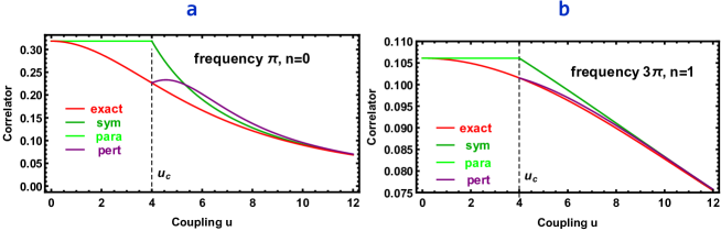
Figure 1: Imaginary part of the correlator for quantum dot at half filling in wide range of couplings u=U/T. Matsubara frequency is $\omega_{n}=\pi T\left(2n+1\right)=\pi$, at $n=0,$ $T=1$. The red line is the exact result, the green line is the Hartree Fock result, the darker green line is the symmetrized green function Eq.(35) for the magnetic phase, and the purple line is the perturbative correction to gaussian approximation (PCGA) Eqs.(65),(66).

IV Application to the antiferromagnetic SRO in the half filled Hubbard model

IV.1 The Hubbard model.

The single band Hubbard model for strongly interacting electrons is defined on $D$ dimensional hypercubic lattice compactified in all directions into a circle of perimeter $N_{s}$. The tunneling amplitude to the neighbouring site is denoted in literature by $t$. We chose it to be the unit of energy $t=1$. Similarly the lattice spacing sets the unit of length $a=1$ and $\hbar=1$. The Hamiltonian is (restricting for notational simplicity to one band and $D=1$, although generalization to arbitrary $D$ and other types of lattices is straightforward):

$$H=\sum\nolimits_{x=1}^{N_{s}}\left\{-\left(a_{x}^{\alpha\dagger}a_{x+1}^{\alpha}+h.c.\right)-\mu n_{x}+Un_{x}^{\upharpoonleft}n_{x}^{\downarrow}\right\}\text{.}$$ (36)

The chemical potential $\mu$ and the on - site repulsion energy $U$ are therefore given in units of the hopping energy. The spin index takes two values $\alpha=\uparrow,\downarrow$. The density and its spin components are $n_{x}=n_{x}^{\upharpoonleft}+n_{x}^{\downarrow}$ with $n_{x}^{\alpha}\equiv a_{x}^{\alpha\dagger}a_{x}^{\alpha}$ respectively. It is well known that at half filling $\mu=\frac{U}{2}$ due to the particle - hole symmetryKorepin . Approximations we will use are “covariant”CCA and thus respect this restriction.

The discretized Matsubara action isNO ,

$$\mathcal{A}=\tau\sum\nolimits_{t,x}\frac{1}{\tau}\left(\psi_{t+1,x}^{\alpha\ast}\psi_{t,x}^{\alpha}-\psi_{t,x}^{\alpha\ast}\psi_{t,x}^{\alpha}\right)\ -\frac{1}{2}\left(\psi_{t,x}^{\alpha\ast}\psi_{t,x+1}^{\alpha}+\psi_{t,x}^{\alpha\ast}\psi_{t,x-1}^{\alpha}\right)-\mu n_{x}-U\psi_{t,x}^{\upharpoonleft\ast}\psi_{t,x}^{\downarrow\ast}\psi_{t,x}^{\upharpoonleft}\psi_{t,x}^{\downarrow}\text{,}$$ (37)

where $n_{t,r}\equiv\psi_{t,x}^{\sigma\ast}\psi_{t,x}^{\sigma}$. Generally for $D\leq 2$ and the nonabelian symmetry group symmetry fluctuations (quantum and thermal) destroy numerous “mean field broken” phases, although previously attempted variational approaches like the CGA at large coupling start from a “broken” phase solution of the minimization equations sometimes give a much better result upon symmetrization. The start from recounting the well known HF gap equation and its paramagnetic solutionAuerbach .

IV.2 The paramagnetic Hartree - Fock solution

The hopping matrix and interaction in frequency-momentum space of the corresponding Matsubara action, is:

$$t_{n,k}^{\alpha\beta} = \delta^{\alpha\beta}t_{n,k};\text{ \ }t_{n,k}=\varepsilon_{m}-2\cos\left[\frac{2\pi}{N_{s}}k\right]\text{,}$$ (38)

$$v_{n,k}^{\alpha\beta} = U\text{.}$$

The gap equation in paramagnet simplifies to

$$\Sigma=-U\frac{T}{N_{s}}\sum\nolimits_{m,k}g_{mk}\text{,}$$ (39)

and is solved numerically (for infinite $N_{t}$) for $T=0.2$. For half filling, $\mu=\frac{U}{2}$, the solution of the above equation is $\Sigma=\frac{U}{2}$. The results for the imaginary part of the correlator $g_{mk}$ presented for $N_{s}=4$ in Fig. 2 as the green line for couplings not exceeding the spurious critical value of $U_{c}\approx 1.3335$. Frequency is the lowest, $n=0$ corresponding to $\omega=\pi T$, while quasimomentum $k=0$ in Fig. 2 and $k=N_{s}/4=1$ ($k$ - vector $\pi/\left(2a\right)$ in physical units) in Fig. 3 but post gaussian correction, or the perturbative correction to gaussian approximation, PCGA is good (PCGA theory will be presented in Sec. VA). As for the quantum dot, it (case for $N_{s}=4$ ) also does not compare well with the exact diagonalization result (red line) for coupling that is not very small. The real part of the correlator on the Fermi surface for $k=\pi/2$ is zero.

Similar results are obtained for other physical quantities at $D=1$, while generalization to $2D$ gives results presented in Fig. 8 that will be commented below. The problem for $U<U_{c}$ is easily remedied by a perturbative correction described in Section IV.

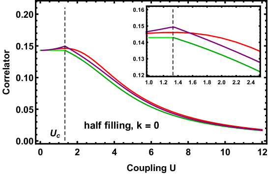
Figure 2: Comparison of the exact correlator of a short Hubbard chain at temperature $T=0.2$ with approximations in wide range of couplings for $\omega=\pi T$, $k=0$. The approximations include the CGA (green lines, the para solution from Eq.(39), darker green lines from Eq.(56)) that is symmetrized above the spurious transition at $U_{c}=1.33$, and perturbative correction to gaussian approximation (PCGA, purple lines).

IV.3 Symmetrized anti - ferromagnetic Green’s function

IV.3.1 Spin rotation and translation spurious symmetry breaking on the HF level

The spin $SU\left(2\right)$ symmetry of the Hubbard model at half filling and large $U$ is spontaneously broken on the HF level to its $U\left(1\right)$ subgroup chosen here as rotation around the $z$ spin direction. Simultaneously the translation symmetry is broken, so that two sublattices $I=1,2$ appear. Therefore translational symmetry becomes smaller with unit cell index $x^{\prime}=1,...,N^{\prime}$ with $N^{\prime}=N_{s}/2$. The position for the sublattice $1$ is $x=2x^{\prime}-1$, while for sublattice $2$ becomes $x=2x^{\prime}$. The Matsubara action therefore is rearranged as a “folded” one:

$$A = \tau\sum\nolimits_{t,x^{\prime}}\frac{1}{\tau}\left(\psi_{t-1,x^{\prime}}^{I\sigma\ast}\psi_{t,x^{\prime}}^{I\sigma}-\psi_{t,x^{\prime}}^{I\sigma\ast}\psi_{t,x^{\prime}}^{I\sigma}\right)-\psi_{t,x^{\prime}}^{I\sigma\ast}\sigma_{x}^{IJ}\psi_{t,x^{\prime}}^{J\sigma}-\frac{1}{2}\psi_{t,x^{\prime}}^{I\sigma\ast}\left(\sigma_{x}^{IJ}+i\sigma_{y}^{IJ}\right)\psi_{t,x^{\prime}-1}^{J\sigma}$$

$$-\frac{1}{2}\psi_{t,x^{\prime}}^{I\sigma\ast}\left(\sigma_{x}^{IJ}-i\sigma_{y}^{IJ}\right)\psi_{t,x^{\prime}+1}^{J\sigma}-\frac{U}{2}n_{i}^{I}+U\psi_{t,x^{\prime}}^{I\upharpoonleft\ast}\psi_{t,x^{\prime}}^{I\downarrow\ast}\psi_{t,x^{\prime}}^{I\upharpoonleft}\psi_{t,x^{\prime}}^{I\downarrow}$$

Here summation over sublattice indices $I,J$ is assumed. The Fourier transform now takes a form

$$\psi_{it}^{I\sigma\ast}=\sqrt{\frac{T}{N^{\prime}}}\sum\nolimits_{k^{\prime}=1}^{N^{\prime}}\sum\nolimits_{n=1}^{N_{t}}\exp\left[i\left(-\frac{2\pi k^{\prime}}{N^{\prime}}i-\frac{2\pi\left(n+1/2\right)}{N_{t}}t\right)\right]\psi_{k^{\prime}n}^{I\sigma\ast}$$ (41)

folded integer quasimomentum $k^{\prime}=1,...,N^{\prime}$. The action becomes that of Eq.(2) with

$$t_{nk^{\prime}}^{-1} = \delta^{IJ}\varepsilon_{n}-\left(1+\cos\left[\frac{2\pi}{N^{\prime}}k^{\prime}\right]\right)\sigma_{x}^{IJ}-\sin\left[\frac{2\pi}{N^{\prime}}k^{\prime}\right]\sigma_{y}^{IJ};$$ (42)

$$v_{nk^{\prime}}^{JI\alpha\beta} = U\delta^{IJ},$$

where $\varepsilon_{n}$ was defined in Eq.(14).

The gap equation, Eq.(6), now take the following form:

$$\Sigma^{IJ\alpha\beta}=\frac{TU}{N^{\prime}}\delta^{IJ}\sum\nolimits_{nk^{\prime}}\left(\delta^{\alpha\beta}g_{nk^{\prime}}^{II\kappa\kappa}-g_{nk^{\prime}}^{II\beta\alpha}\right)=U\delta^{IJ}\left(\delta^{\alpha\beta}n^{II\kappa\kappa}-n^{II\beta\alpha}\right)\text{.}$$ (43)

As is well known, it is solved by the anti - ferromagnetic (AF) Ansatz

$$n^{11\uparrow\uparrow} = n^{22\downarrow\downarrow}=n_{1};n^{11\downarrow\downarrow}=n^{22\uparrow\uparrow}=n_{2};$$ (44)

$$n^{11\uparrow\downarrow} = n^{11\downarrow\uparrow}=n^{22\uparrow\downarrow}=n^{22\downarrow\uparrow}=0\text{.}$$

The resulting algebraic equations at infinite $N_{t}$ are $n_{1}+n_{2}=1$, and, defining magnetization, $M=n_{1}-\frac{1}{2}$,

$$\sum\nolimits_{k^{\prime}=1}^{N^{\prime}}\frac{1}{e_{k^{\prime}}}\tanh\left[\frac{e_{k^{\prime}}}{2T}\right]=\frac{N_{s}}{U};$$ (45)

$$e_{k^{\prime}}^{2}=4\cos^{2}\left[\frac{2\pi}{N_{s}}k^{\prime}\right]+\left(UM\right)^{2}\text{.}$$

The spurious critical coupling therefore is:

$$U_{c}\left(T\right)=2N_{s}\left\{\sum\nolimits_{k^{\prime}=1}^{N^{\prime}}\cos^{-1}\left[\frac{2\pi}{N_{s}}k^{\prime}\right]\tanh\left[\frac{2\cos\left[\frac{2\pi}{N_{s}}k^{\prime}\right]}{2T}\right]\right\}^{-1}\text{.}$$ (46)

For particular cases shown in Figs. 2,3 and 5, we set $N_{s}=4$ and $24$ respectively. The values of the critical coupling at temperature $T=0.2$ are $U_{c}=1.3335$ and $U_{c}=2.017$ at half filling respectively.

The nonsymmetrized correlator is diagonal in spin, $g_{nk^{\prime}}^{IJ\uparrow\downarrow}=$ $g_{nk^{\prime}}^{IJ\downarrow\uparrow}=0$, due to the residual $U\left(1\right)$ symmetry, so we specify the spin $\alpha$ once:

$$g_{nk^{\prime}}^{IJ\alpha}=\frac{1}{e_{k^{\prime}}^{2}+\omega_{n}^{2}}\left\{\left(1+\cos\left[\frac{2\pi}{N^{\prime}}k^{\prime}\right]\right)\sigma_{x}^{IJ}-\sin\left[\frac{2\pi}{N^{\prime}}k^{\prime}\right]\sigma_{y}^{IJ}+i\omega_{n}\delta^{IJ}-sgn\left[\alpha\right]UM\sigma_{z}^{IJ}\right\}\text{.}$$ (47)

Here $sgn\left[\alpha\right]=\sigma_{z}^{\alpha\alpha}$, namely $+1$ for $\uparrow$ and $-1$ for $\downarrow$. Recall that we have chosen the direction of magnetization at large coupling in the spuriously broken phase to be parallel to the $z$ spin direction. This should be symmetrized over all the AF ground states.

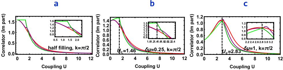
Figure 3: Comparison of the exact correlator of a short Hubbard chain at temperature $T=0.2$ with approximations in wide range of couplings for $\omega=\pi T$, $k=\pi/2$ at $\delta\mu=0,0.25,1$ from top to bottom. The approximations include the CGA (green lines, the para solution from Eq.(39), darker green lines from Eq.(56)) that is symmetrized above the spurious transition at $U_{c}=1.33$, and perturbative correction to gaussian approximation in Fig.3a (PCGA, purple lines). The inset of Fig.3a is an enlarged figure near the “critical coupling” region. Fig.3b and Fig.3c ($\delta\mu=0.25,1$ respectively), the results for the CGA (green lines for para solution, darker green lines from the symmetrized correlator) are present, the exact results are plotted as red lines.

IV.3.2 Symmetrization

Then symmetry breaking pattern for the $SU\left(2\right)\rightarrow U\left(1\right)$ for the paramagnet to AF involves simultaneous translation symmetry breaking resulting in sublattices. Taking trace over spins and dividing by $2$, the symmetrized frequency - quasimomentum GF is:$\left\langle\psi_{nx}^{\ast\uparrow}\psi_{ny}^{\uparrow}\right\rangle\approx\frac{1}{2}\left\langle\psi_{nx}^{\ast\sigma}\psi_{ny}^{\sigma}\right\rangle_{AF}=\frac{1}{2}\left(\left\langle\psi_{nx}^{\ast\uparrow}\psi_{ny}^{\uparrow}\right\rangle_{AF}+\left\langle\psi_{nx}^{\ast\downarrow}\psi_{ny}^{\downarrow}\right\rangle_{AF}\right)$ ($n$ is the Matsubara frequency, $x,y$ are the lattice coordinates)

$$g_{nk}^{sym} = \frac{1}{N_{s}}\sum\nolimits_{x,y=1}^{N_{s}}\exp\left[\frac{2i\pi k}{N_{s}}\left(x-y\right)\right]\left\langle\psi_{nx}^{\ast\uparrow}\psi_{ny}^{\uparrow}\right\rangle$$ (48)

$$\approx \frac{1}{2N_{s}}\sum\nolimits_{x,y=1}^{N_{s}}\exp\left[\frac{2i\pi k}{N_{s}}\left(x-y\right)\right]\left\langle\psi_{nx}^{\sigma\ast}\psi_{ny}^{a\sigma}\right\rangle_{AF}\text{.}$$ (49)

In sublattice notations this becomes:$\left\langle\psi_{nx}^{\ast\uparrow}\psi_{ny}^{\uparrow}\right\rangle\approx\frac{1}{2}\left(\left\langle\psi_{nx}^{\ast\uparrow}\psi_{ny}^{\uparrow}\right\rangle_{AF}+\left\langle\psi_{nx+1}^{\ast\uparrow}\psi_{ny+1}^{\uparrow}\right\rangle_{AF}\right)$

$$g_{nk}^{sym} = \frac{1}{4N^{\prime}}\sum\nolimits_{x^{\prime}y^{\prime}}^{N^{\prime}}\exp\left[\frac{2i\pi k}{N^{\prime}}\left(x^{\prime}-y^{\prime}\right)\right]\left\{\begin{array}[]{c}\left\langle\psi_{nx^{\prime}}^{1\sigma\ast}\psi_{ny^{\prime}}^{1\sigma}\right\rangle+\exp\left[-\frac{i\pi k}{N^{\prime}}\right]\left\langle\psi_{nx^{\prime}}^{1\sigma\ast}\psi_{ny^{\prime}}^{2\sigma}\right\rangle\\ +\exp\left[\frac{i\pi k}{N^{\prime}}\right]\left\langle\psi_{nx^{\prime}}^{2\sigma\ast}\psi_{ny^{\prime}}^{1\sigma}\right\rangle+\left\langle\psi_{nx^{\prime}}^{2\sigma\ast}\psi_{ny^{\prime}}^{2\sigma}\right\rangle\end{array}\right\}$$ (52)

$$= \frac{1}{4}\left\{\begin{array}[]{c}\left\langle\psi_{n,\text{mod}\left[k\right]}^{1\sigma\ast}\psi_{n,\text{mod}\left[k\right]}^{1\sigma}\right\rangle+\exp\left[-\frac{i\pi k}{N^{\prime}}\right]\left\langle\psi_{n,\text{mod}\left[k\right]}^{1\sigma\ast}\psi_{n,\text{mod}\left[k\right]}^{2\sigma}\right\rangle\\ +\exp\left[\frac{i\pi k}{N^{\prime}}\right]\left\langle\psi_{n,\text{mod}\left[k\right]}^{2\sigma\ast}\psi_{n,\text{mod}\left[k\right]}^{1\sigma}\right\rangle+\left\langle\psi_{n,\text{mod}\left[k\right]}^{2\sigma\ast}\psi_{n,\text{mod}\left[k\right]}^{2\sigma}\right\rangle\end{array}\right\}$$

$$= \frac{1}{4}\left\{g_{n,\text{mod}\left[k\right]}^{11\sigma}+g_{n,\text{mod}\left[k\right]}^{22\sigma}+\exp\left[-\frac{2i\pi k}{N_{s}}\right]g_{n,\text{mod}\left[k\right]}^{12\sigma}+\exp\left[\frac{2i\pi k}{N_{s}}\right]g_{n,\text{mod}\left[k\right]}^{21\sigma}\right\}\text{,}$$

where $\text{mod}\left[k\right]=\text{mod}\left[k,N^{\prime}\right]=\text{mod}\left[k,N_{s}/2\right]$.

Substituting the solution of the gap equation, one finally obtains, for half filling:

$$g_{nk}^{sym}=\frac{i\omega_{n}+2\cos\left[\frac{2\pi}{N_{s}}k\right]}{\omega_{n}^{2}+e_{\text{mod}\left[k\right]}^{2}}\text{.}$$ (56)

An example of results is compared with exact diagonalization for $N_{s}=4,T=0.2$ for $n=0$ and $k=0,N_{s}/4$ (corresponding to physical momentum $\pi/2$) in Figs. 2 and 3a respectively. The symmetrized broken phase solution (the dark green curve) for $U>U_{c}\left(T\right)\$provides a quite accurate approximant. It approaches the exact result at large coupling although still incorrectly indicates the second order transition (see the cusps in inserts of both Figs. 2 and 3). The most problematic values of both the frequency, $\omega=\pi T$ and the quasimomentum $k=0$ and $N_{s}/4$ (Fermi surface) are chosen. The other physical quantities are discussed in Section VI.

A question arises. Since qualitative features are captured quite well by the symmetrized CGA except near the spurious transition, can one improve upon this using the CGA as a starting point of a perturbation? This is attempted next.

V Perturbative improvement of the gaussian theory

V.1 General construction of the series

The covariant gaussian approximation can serve as a starting point for a perturbation theory around the Hartree - Fock solution. In bosonic models the method was proposed in the context of strong thermal fluctuations in the mixed state of superconductor under magnetic fieldThouless . One considers the quadratic form,

$$\mathcal{A}_{g}=-\psi_{a}^{A\ast}\left[G^{-1}\right]_{b-a}^{BA}\psi_{b}^{B}\text{,}$$ (57)

as a “large” part of the action, while the difference between the models action Eq.(2) and it is “small”. The small part is multiplied by a parameter $\alpha$ and the physical quantity is expanded in $\alpha$ to a certain order. After the calculation is completed one sets $\alpha=1$.

The gaussian action for an interacting electron system is (as before the space index combined with time):

$$\mathcal{A} = \mathcal{A}_{g}+\alpha\Delta\mathcal{A}\text{;}$$ (58)

$$\Delta\mathcal{A}\text{ } = \frac{1}{2}\psi_{a}^{A\ast}\psi_{a}^{A}V_{a-b}^{AB}\psi_{b}^{B\ast}\psi_{b}^{B}+\psi_{a}^{A\ast}\left(T_{a-b}^{AB}+\left[G^{-1}\right]_{b-a}^{BA}\right)\psi_{b}^{B}\text{.}$$

Integrands in the path integral are expanded as

$$e^{-\left(\mathcal{A}_{g}+\alpha\Delta\mathcal{A}\right)}=e^{-\mathcal{A}_{g}}\left(1-\alpha\Delta\mathcal{A}+\frac{1}{2}\alpha^{2}\left(\Delta\mathcal{A}\right)^{2}+..\right)\text{.}$$ (59)

The correlator therefore is expanded to $\alpha$ as

$$\left\langle\psi_{a}^{A\ast}\psi_{b}^{B}\right\rangle = \frac{\int\psi_{a}^{A\ast}\psi_{b}^{B}e^{-\mathcal{A}_{g}}\left(1-\alpha\Delta\mathcal{A}+\frac{1}{2}\alpha^{2}\left(\Delta\mathcal{A}\right)^{2}\right)}{\int e^{-\mathcal{A}_{g}}\left(1-\alpha\Delta\mathcal{A}+\frac{1}{2}\alpha^{2}\left(\Delta\mathcal{A}\right)^{2}\right)}$$

$$\approx G_{ab}^{AB}+\alpha\left\langle\psi_{a}^{A\ast}\psi_{b}^{B}\text{ }\Delta\mathcal{A}\right\rangle_{con}+\frac{\alpha^{2}}{2}\left\langle\psi_{a}^{A\ast}\psi_{b}^{B}\left(\Delta\mathcal{A}\right)^{2}\right\rangle_{con}$$

$$= G_{ab}^{AB}+\alpha^{2}\Delta G_{ab}^{AB}\text{.}$$

The $\left\langle...\right\rangle_{con}$ average is understood in a diagrammatic representation of the gaussian integrals as in perturbation theoryNO (division by $Z$ eliminates disconnected diagrams). Vanishing of the $\alpha$ term is tantamount to solution of the gap equation, Eq.(6), as shown in ref.Thouless, (no difference here between bosonic and fermionic models). $G_{ab}^{AB}$ is the green function of Gaussian (Hartree-Fock) approximation.

The correction to the Gaussian correlator $G_{ab}^{AB}$ is (setting $\alpha=1$ and simplifying by repeated use of the gap equation)

$$\Delta G_{ab}^{AB}=G_{ak}^{AK}V_{kl}^{KL}G_{nl}^{NL}\left(G_{kn}^{KN}G_{lm}^{LM}-G_{km}^{KM}G_{ln}^{LN}\right)V_{mn}^{MN}G_{mb}^{MB}\text{.}$$ (61)

It is known that within gaussian approximation the effective action is calculated much more precisely compared to correlatorsKleinert . The cumulant ( the inverse of the green function that is the second functional derivative of the effective action with respect to field) within the first order is given by a simpler formula:

$$\left[\left(G^{pg}\right)^{-1}\right]_{ab}^{AB} = \left[G^{-1}\right]_{ab}^{AB}+\Sigma_{ab}^{AB};$$ (62)

$$\Sigma_{ab}^{AB} = V_{al}^{AL}G_{nl}^{NL}\left(G_{ab}^{AB}G_{ln}^{LN}-G_{an}^{AN}G_{lb}^{LB}\right)V_{bn}^{BN}\text{.}$$

Here $\Sigma_{ab}^{AB}$ is self energy correction to the Gaussian correlator, and $G^{pg}$ is the green function of post (perturbative correction) gauss approximation (PCGA). Diagrammatically it can be represented as summation of all the “setting sun” diagrams with lines representing the gaussian correlators, see Fig. 4.

Figure 4: Setting sun diagrams that contribute to PCGA. The directed lines are gaussian correlators, while the vertices are “perturbative”.

As an example we calculate the first correction (“perturbed” or “setting sun” approximation) to the toy model of Section II. For the QD model, substituting Eq.(13) into Eq.(62), one obtains (using the property of both the paramagnetic and the ferromagnetic solutions that $G^{AB}$ is diagonal in spin due to the residual $U\left(1\right)$ symmetry),

$$\Sigma_{ab}^{AA}=\tau^{2}U^{2}G_{ba}^{\overline{A}\overline{A}}G_{ab}^{AA}G_{ab}^{\overline{A}\overline{A}}\text{.}$$ (63)

Transforming to frequencies, one obtains,

$$\Sigma_{n}^{AA}=T^{2}U^{2}\sum\nolimits_{k,l}g_{-n+k+l}^{\overline{A}\overline{A}}g_{k}^{AA}g_{l}^{\overline{A}\overline{A}}\text{,}$$ (64)

so that in paramagnet, Eq.(34), for infinite $N_{t}$, $\left[\gamma_{CGA}^{-1}\right]^{AB}=\delta^{AB}g^{CGA}$ with

$$g_{n}^{CGA}=i\left\{\omega_{n}+U^{2}T^{2}\sum\nolimits_{k,l=-\infty}^{\infty}\frac{1}{\omega_{k+l-n}\omega_{k}\omega_{l}}\right\}^{-1}\text{.}$$ (65)

The sum can be performed resulting in the exact expression given in Eq.(34). The calculation of the setting sun correction in the magnetic phase is more complicated, however the result is simple (after symmetrization):

$$g_{n}^{pert}=i\omega_{n}\frac{U^{2}/4+\omega_{n}^{2}}{\left(2UM\omega_{n}\right)^{2}+\left(2U^{2}M^{2}-U^{2}/4-\omega_{n}^{2}\right)^{2}}\text{.}$$ (66)

Here magnetic moment $M$ is determined by the gap equation Eq.(23). The correlator of Eq.(66) is plotted as the purple line in Fig. 1. The most difficult case of $\omega=\pi T$ is given in Fig.1. One observes that it significantly improves the symmetrized CGA near the spurious transition at $U_{c}$ (see inset), but is not effective at higher couplings. If $U<U_{c}$, the perturbative correction turns out to be exact. The asymptotics for large coupling is correct and corrections are exponential. The improvement is dramatic for larger frequencies, as can be seen from Fig.1b.

V.2 Perturbative correction to gaussian approximation in the Hubbard model

Applying the general formula for the setting sun corrected self energy, Eq.(62) in the anti - ferromagnetic phase of the Hubbard model, one obtains:

$$\Sigma_{\alpha}^{\upharpoonleft IJ} = \frac{T^{2}U^{2}}{N^{\prime}}\sum\nolimits_{\chi_{1},\chi_{2}}G_{\chi_{1}}^{\upharpoonleft IJ}G_{\chi_{2}}^{\downarrow IJ}G_{\chi_{1}+\chi_{2}-\alpha}^{\downarrow JI}\text{,}$$ (67)

$$\Sigma_{\alpha}^{\downarrow IJ} = \frac{T^{2}U^{2}}{N^{\prime}}\sum\nolimits_{\chi_{1},\chi_{2}}G_{\chi_{1}}^{\downarrow IJ}G_{\chi_{2}}^{\upharpoonleft IJ}G_{\chi_{1}+\chi_{2}-\alpha}^{\upharpoonleft JI}$$

where $I,J$ are sublattice indices, $\alpha,\chi$ indices are the combined indices of frequency and wavevector. Substituting the HF anti - ferromagnetic solution of Eq.(45) in the matrix form the correlator is:

$$G_{nk}^{\sigma}=\frac{1}{\omega_{n}^{2}+4\cos^{2}\left[\frac{2\pi k}{N_{s}}\right]+M^{2}U^{2}}\begin{pmatrix}i\omega_{n}+\left(-\right)^{\sigma}MU&1+\exp\left[4i\pi k/N_{s}\right]\\ 1+\exp\left[-4i\pi k/N_{s}\right]&i\omega_{n}-\left(-\right)^{\sigma}MU\end{pmatrix}\text{.}$$ (68)

where $\sigma$ is the spin index, and for spin up $\sigma=1$, spin down $\sigma=2$. Using Eq.(62), the PCGA correlators are obtained and the symmetrization of the PCGA correlators follows. The symmetrized PCGA correlators are plotted in the different figures of the present paper using purple lines or points. The generalization to higher dimensions, different dispersion relations/lattices, beyond half filling etc is straightforward.

These results are systematically compared with exact and Monte Carlo simulations in the 1D Hubbard model in the next section and with 2D Hubbard model in Section V.

VI Comparison with exact diagonalization and the Monte Carlo simulation of the Hubbard Model

Exact solutions of strongly interacting electron systems are scarce. This especially true for Green’s function at finite temperature. We use exact diagonalizationED in 1D for small lattice at any filling (standard and thus not described here) and then utilize the determinant quantum Monte Carlodqmc (DQMC, briefly described in Appendix) for half filling only. Although the methodology has been extended recently to approach electronic systems beyond the half filling, for the benchmarks purpose we stay with well established half filling domain for which the sign problem was shown to be nonexistent.

VI.1 Coupling and quasi - momentum dependence of the Green’s function of half filled Hubbard chain

In this subsection our analytic results are compared with exact diagonalization of the 1D half filling in the most troublesome case of half filling (appears as red lines in figures). Results beyond half filling are in far better agreement with exact even for deviation as small as $\delta\mu=\mu-U/2=0.1$. At half filling, the imaginary part of the Green’s function at quasimomentum in the $\Gamma$ point, $k=0$, and on the Fermi surface $k=1$ (corresponding to the physical wave vector $\pi/2$) is shown on Fig. 2 and Fig.3a respectively for $N_{s}=4$. The results are for fixed temperature (in units of hopping energy $t=1)$, $N_{s}=4$, and at lowest Matsubara frequency $\omega_{n=0}=\pi T$ (by far the most difficult case, as example of the simpler model demonstrates, see Fig.1). The range of couplings $U_{c}<U<12$ is shown with inset magnifying the region around the spurious critical value $U_{c}=1.3335$ marked by the dashed line for $T=0.2$ in Fig. 2 and Fig. 3a for $T=0.2$, $N_{s}=4$. All the calculations here are for infinite $N_{t}$. In Figs. 3a, 3b, 3c imaginary part of the Green’s function at quasimomentum $k=1$ (corresponding to the physical wave vector $\pi/2$) is shown respectively for $\delta\mu=0$, $\delta\mu=0.25$ and $\delta\mu=1$.

Below the spurious phase transition HF (green straight segment) deviates significantly from the exact diagonalization result (red curve), especially near $U_{c}$. However well above $U_{c}$ the symmetrized CGA result (green curve) compares well with the exact correlator. On the Fermi surface, $k=\pi/2$, the perturbative improvement over the symmetrized CGA (the purple curve in Figs.2, 3a) is significant not just near the spurious transition at $U_{c}$, but all the way to the large $U$ limit. The leading large $U$ asymptotic, $g=\frac{4\pi T}{U^{2}}$($\frac{2.51}{U^{2}}$for $T=0.2$) is captured correctly by both CGA and the perturbatively improved CGA for both quasimomentum $k=0,\pi/2$. However the coefficient $c$ of the subleading, $c/U^{4}$, correction (powers are even due to the particle - hole symmetry) is different. The exact one for $k=0$ is $c=40.6$, while approximate are $c=-24.1$ and $c=-8.5$ for CGA and the perturbatively corrected CGA (PCGA) respectively. For $k=\pi/2$ the situation is similar: exact $c=86.0$, while CGA and PCGA give $c=29.8$ and $c=-27.8$ correspondingly. The conclusion is that for very strong antiferromagnetic state the dominant correlation is antiferromagnetic and the long range symmetrization is less important. The perturbation thus is not helpful in this respect. Its main advantage is at intermediate couplings. The most important positive observation is that symmetrized mean field works better beyond half filling.

However, in the case of QD, the large $U$ limit expansion (polynomial expansion $U^{-2k},k=1,2..$) of the correlator from Eq.(66) is the same as the exact one, and the difference between them is exponential small factor ($e^{-0.5U}$).

For large $N_{s}$ the exact diagonalization is impossible and thus DQMC was used as a benchmark. We present next comparison of the quasimomentum distribution for large enough chain, so that the continuum limit is reached.

Figure 5: The quasi - momentum distribution function $n_{k}=2T\sum\limits_{m}g\left(m,k\right)$ in half filled 1D Hubbard model ($N_{s}=24$). factor $2$ is due to spin summation. horizontal axis as $k$ is quas-momentum, and quantized as in unit $2\pi/N_{s}$, and the plot range of $k$ is from $0$ to $\pi$. The results for CGA (green dots), and PCGA (purple dots) are plotted along with MC results (red lines).

VI.2 Distribution of momenta in 1D Hubbard model

In Fig. 5 the coupling dependence of the distribution function $n_{k}$ of the $N_{s}=24$ Hubbard chain are compared with determinant quantum Monte Carlo simulation (red line), see Appendix for details. Temperature is again fixed at $T=0.2$, while couplings are $U=1,4,6,10$. The spurious transition occurs at $U_{c}=2.017$ very close to the value mean field transition point $U_{c}=2.0186$ in the thermodynamic limit $N_{s}=\infty$, so that it essentially represents the continuum limit. We use the infinite $N_{t}$ limit for the symmetrized HF (green points) and PCGA (purple points).

One observes that at the weak coupling ($U=1$) the agreement is excellent and the perturbation improves significantly the gaussian result. The weak coupling limit comparison means that the MC simulation time slice corresponding to $N_{t}=40$ is precise enough. For an intermediate coupling above $U_{c}$ ($U=4,6$) there are deviations of up to $10\%$ at certain momenta, that are only modestly corrected perturbatively. Finally at strong coupling ($U=10$) the agreement is good, but the perturbative correction does not help much.

VI.3 Charge and spin correlators in 1D Hubbard model

In this subsection more complicated correlators of the Fermionic fields are compared with exact results on small lattice and Monte Carlo simulations of the half filled model on larger ones.

In Fig. 6 the coupling dependence of the charge density correlator $\chi_{n,k}^{\rho}=\left\langle n_{n,k}n_{-n,-k}\right\rangle$ of the $N_{s}=4$ Hubbard chain at half filling is compared with the exact diagonalization (red line). The subindices $n,k$ of $n_{n,k}$ corresponds to Matsubara frequency $\omega_{n}=\pi T\left(2n+1\right)$, $k$ is the quasi-momentum, $n_{n,k}$ is the Fourier transformations of the density $n_{\tau,x}$. Temperature is fixed at $T=1$, frequency at $n=0$, momentum at $k=0$, while the coupling range is $U=0-12$. The spurious transition occurs at $U_{c}=4.541$. The symmetrized density correlator (the customary Lindhard diagram with propagators given by the HF approximation, green lines) deviates from exact result near the spurious transition, although it has a correct asymptotics at both weak and strong couplings.

The one vertex corrected symmetrized density correlator (purple points) does better. It is within 1% in the “unbroken” phase (including the spurious transition point), and improves the intermediate region. Inset demonstrates the ration of an approximate and the exact correlator at large coupling.

Figure 6: The charge density correlator $\chi^{\rho}=$ $\chi_{n,k}^{\rho}$ dependence of $U$ at $T=1.$, for frequency $n=0$, momentum at $k=0$. The green curve is the Lindhard diagram result, and the purple curve contains in addition the next order correction to the Lindhard diagram. The green curve and the purple curve in the inset are the ratios between the Lindhard result and the result including the next order correction to the exact value respectively.

Figure 7: The spin correlator $\chi_{n}^{s}=\left\langle\overrightarrow{S}_{n,x}\cdot\overrightarrow{S}_{-n,x}\right\rangle$ dependence of $U$ at $T=1$ for frequency $n=0$. The green curve is the Lindhard diagram result, and the purple curve contains in addition the next order correction to the Lindhard diagram.

Another interesting correlator is the spin correlator $\chi_{n,k}^{s}=\left\langle\overrightarrow{S}_{n,k}\cdot\overrightarrow{S}_{-n,-k}\right\rangle$. The subindices $n,k$ of $\overrightarrow{S}_{n,k}$ corresponds to Matsubara frequency $\omega_{n}=\pi T\left(2n+1\right)$, $k$ is the quasi-momentum, and $\overrightarrow{S}_{n,k}$ is the Fourier transformations of the spin $\overrightarrow{S}_{\tau,x}$.  Parameters $N_{s}$, $T$ are the same as for the density correlator, frequency still at $n=0$, but instead of quasimomentum we take the coincident point correlator $\chi_{n}^{s}=\left\langle\overrightarrow{S}_{n,x}\cdot\overrightarrow{S}_{-n,x}\right\rangle$ for $n=0$. The results are presented in Fig. 7 as function of the coupling in the range $U=0-16$. The approximation quality is approximately (a little worse than density correlator) the same as in the previous case of the density correlator. For results of large $N_{s}$, we will present the results in the future works.

Figure 8: Imaginary part of the Green’s function $G\left(\tau,\mathbf{k}\right)$ of half filled 2D Hubbard model at $k=\left(\pi,0\right)$. The results for CGA (green dots), and PCGA (purple dots) are plotted along with MC results (red lines).

VI.4 Comparison of MC simulation with CGA in 2D Hubbard model

Calculations for half filled Hubbard model in 2D are completely analogous to those in 1D. In Fig. 8 the coupling dependence of the Matsubara Green’s function at the point $k=\left(\pi,0\right)$ on the Fermi surface is plotted as function of Matsubara time. As was demonstrated in the previous subsection, momenta on the Fermi surface are most difficult to describe. The temperature is fixed at $T=1$, and only half of the period $0<t<1/\left(2T\right)$ is shown since the other half is dictated by the symmetry. The number of space points was $144$ with $N_{s}=12$ in the DQMC simulation (red line), while the time slice corresponds to $N_{t}=8$, see more detailed description of methodology in Appendix. The couplings, $U=1,4,6,8,12$, were taken below and above the spurious mean field transition at $U_{c}=4.90$. We use the infinite $N_{t}$ limit for the symmetrized HF (green points) and PCGA (purple points).

One observes that at the weak coupling ($U=1,4$) below $U_{c}$ the agreement is excellent only if the HF (the green vertical line) is perturbatively corrected as in 1D. The weak coupling limit comparison means that the MC simulation time slice corresponding to $N_{t}=8$ is precise enough. For an intermediate coupling just above $U_{c}$ ($U=6$) there are significant deviations of up to $15\%$ , that are not corrected perturbatively. Finally at a stronger couplings ($U=8,12$) the agreement is good, but improvement (perturbative correction) does not help much.

VII Discussion and conclusions

To summarize, a mean field (Hartree-Fock) type approach, covariant gaussian approximation is adapted to include strongly interacting low dimensional electronic systems in which symmetry is “restored” due to long range correlations. Instead of using a complicated (typically renormalization group type) scale separation method, simple symmetrization of correlators is employed to a covariant (preserving Ward - Takahashi identities) variant of the mean field (gaussian) approximation. The short range correlations captured by the mean field are thus kept, while symmetry gets restored. The solution can be systematically improved by addition of corrections to cumulant that are based on expansion around the gaussian approximation. There are different  variational Hartree-Fock methods Tomita which were applied to study the strong correlated model, for example, the Hubbard model with success. However here we offered the traditional (simple analytic) Hartree-Fock methods to calculate the correlators.

To test the scheme, it was applied to the correlator of the 1D and the 2D one band Hubbard models and compared to exact diagonalization of relatively small systems (ED) and MC simulations at the half filling, where they are known to be reliable. The comparison demonstrates the typical mean field precision of order 10% for all couplings. It is better for weak and strong couplings (correct asymptotics) away from the Fermi level and higher frequencies. It should be noted that the method generalizes well beyond half filling Hubbard model. The 2D Hubbard model beyond the half filling that is being intensely studied recently in connection to strange metals and high $T_{c}$ superconductivity (including by the determinantal quantum Monte Carlodqmc used here at half filling only). Apart from straightforward generalizations to different symmetry groups describing for example Ising or XY quantum magnets, possible applications include models describing phonon induced interactions like the Holstein model. For disordered matter, one can combine replica field theory method with the method used in the present paper.

A natural question arises whether the symmetrization scheme can be applied to finer approximations beyond the gaussian. Recently the covariant approximation method was generalized to include higher cumulants beyond the quadraticCCA .

Acknowledgements

Authors are very grateful to J. Wang, B. Shapiro, for numerous discussions and I. Berenstein and G. Leshem for help in computations. B. R. was supported by MOST of Taiwan #107-2112-M-003-012. D. P. L. was supported by National Natural Science Foundation of China (No. 11674007 and No. 91736208). B. R. and D.P.L are grateful to School of Physics of Peking University and The Center for Theoretical Sciences of Taiwan for hospitality respectively.

Appendix A Determinant Quantum Monte Carlo

The determinant quantum Monte Carlo (DQMC) method is an exact numerical tool to treat the correlated system. To apply DQMC simulations in fermion system, a major obstacle is the notorious sign problem, which prevents DQMC simulations from achieving a good numerical precision at low temperature and high interaction strength. However, in the half-filled Hubbard model on a square lattice, the sign problem disappears due to the particle hole symmetry, and this provide a wonderful opportunity to use the data of DQMC as the benchmark for our method.

The DQMC method that we use is based on Blankenbecler–Scalapino–Sugar (BSS) algorithmdqmc . In this Appendix, we present a brief introduction following previous work on the Hubbard modelHirsch . The Hamiltonian Eq.(36) can is separated into $H=H_{0}+H_{I}$ where $H_{0}$ is the hopping part and $H_{I}$ is includes the rest of terms in Eq.(36). In order to calculate the grand partition function $Z=Tr\ e^{-H/T}$, one need to use the Suzuki-Trotter decomposition schemeSuzuki , to cast the quartic term into a bilinear form, and introduce a small parameter $\tau=\left(TN_{t}\right)^{-1}$,

$$e^{-(H_{0}+H_{I})/T}=\left(e^{\tau H_{0}+\tau H_{I}}\right)^{N_{t}}=\left(e^{\tau H_{0}}e^{\tau H_{I}}\right)^{N_{t}}+O\left(\tau^{2}U\right).$$ (69)

Having separated the exponentials, we can decouple the quartic terms in $H_{I}$ by the Hubbard–Stratonovich (HS) transformation,

$$e^{-U\tau n_{\uparrow}n_{\downarrow}}=\frac{1}{2}e^{-\frac{U\tau}{2}n}\sum_{s=\pm 1}e^{-s\xi\left(n_{\uparrow}-n_{\downarrow}\right)}=\frac{1}{2}\sum_{s=\pm 1}\prod_{\sigma=\uparrow,\downarrow}e^{-\left(sgn\left[\sigma\right]s\xi+\frac{U\tau}{2}\right)n_{\sigma}}\text{,}$$ (70)

where $n\equiv n_{\uparrow}+n_{\downarrow}$. and the parameter $\xi=$ arccosh$\left[e^{|U|\tau/2}\right]$. One can notice that the quartic terms are decoupled at the cost of introducing an auxiliary field at every site and time slice. Upon replacing the on-site interaction on every site of the space-time lattice by Eq. (70), we obtain the sought of form in which only bilinear terms appear in the exponential,

$${\mathcal{Z}}=\left(\frac{1}{2}\right)^{N_{s}^{D}N_{t}}\underset{\{s\}}{\text{{\Large{Tr}}}}\prod_{t=1}^{N_{t}}\prod_{\sigma=\uparrow,\downarrow}\exp\left[-\tau H_{0}\right]\exp\left[-\tau\sum_{\mathbf{i}}c_{\mathbf{i}}^{\sigma\dagger}V_{\mathbf{i}}^{\sigma}(t)c_{\mathbf{i}}^{\sigma}\right]$$ (71)

where the traces are over auxiliary Ising fields and over fermion occupancies on every site. The time-slice index $t$ is manifested in the HS field $s_{i}(t)$ by

$$V_{i}^{\sigma}(t)=sgn\left[\sigma\right]\frac{\xi}{\tau}s_{i}(t)+\mu-\frac{U}{2}\text{,}$$ (72)

which are the elements of the $N_{s}\times N_{s}$ diagonal matrix $V^{\sigma}(t)$. With bilinear forms in the exponential, the fermions can be traced out explicitly,

$${\mathcal{Z}}=\left(\frac{1}{2}\right)^{N_{s}^{D}N_{t}}\underset{\{s\}}{\text{{\Large{Tr}}}}\,\prod_{\sigma}\det\left[{\mathbf{1}}+\mathsf{B}^{\sigma}\left(N_{t}\right)\mathsf{B}^{\sigma}\left(N_{t}-1\right)\ldots\mathsf{B}^{\sigma}\left(1\right)\right],$$ (73)

with $\mathsf{B}^{\sigma}\left(t\right)\equiv e^{-\tau K}e^{-\tau V^{\sigma}(t)}$, in which the auxiliary Ising spins are implicitly included. The hopping terms in the exponential are represented by an $N_{s}\times N_{s}$ matrix $K$, with elements

$$K_{ij}=\begin{cases}-1&\text{if $i$ and $j$ are nearest neighbours},\\ 0&\text{otherwise}.\end{cases}$$ (74)

The equal-‘time’ correlation function of the creation and the annihilation operators is:

$$\langle c_{\mathbf{i}}^{\sigma}c_{\mathbf{j}}^{\sigma\dagger}\rangle=\frac{1}{\mathcal{Z}}\,\underset{\{s\}}{\text{{\Large{Tr}}}}T{\text{{\Large$r$}}}\left[c_{\mathbf{i}}^{\sigma}c_{\mathbf{j}}^{\sigma\dagger}\prod_{t,\sigma}e^{-\tau K}e^{-\tau V^{\sigma}(t)}\right]\text{.}$$ (75)

Considering the fact that the fermions only interact with the auxiliary fields, it can be proved that Wick’s theorem FW holds for a fixed HS configuration Hirsch ; vdl92 ; Loh92 . Hence, the interesting physical expectations can be calculated in terms of single-particle Green’s functions. In the ‘Heisenberg picture’, the time-dependent $c$ operator is defined as,

$$c(t)\equiv e^{t\tau H}\,c\,e^{-t\tau H}\text{,}$$ (76)

with the initial time set to be $t=\tau$ and $c^{\dagger}(t)\neq[c(t)]^{\dagger}$. Further, the unequal-time Green’s function, for $t_{1}>t_{2}$, is given by Hirsch

$$G_{\mathbf{i}\mathbf{j}}^{\sigma}(t_{1};t_{2}) \equiv \left\langle c_{\mathbf{i}}^{\sigma}(t_{1})c_{\mathbf{j}}^{\sigma\dagger}(t_{2})\right\rangle_{\{s\}}$$ (77)

$$= \left[\mathsf{B}^{\sigma}\left(t_{1}\right)\mathsf{B}^{\sigma}\left(t_{1}-1\right)\ldots\mathsf{B}^{\sigma}\left(t_{2}+1\right)\,\mathsf{g}^{\sigma}(t_{2}+1)\right]_{\mathbf{i}\mathbf{j}}\text{,}$$

in which the Green’s function matrix at the $t$-th time slice is defined as $\mathsf{g}^{\sigma}(t)\equiv\left[\mathsf{1}+\mathsf{A}^{\sigma}(t)\right]^{-1}$ with $\mathsf{A}^{\sigma}(t)\equiv\mathsf{B}^{\sigma}\left(t-1\right)\mathsf{B}^{\sigma}\left(t-2\right)\ldots\mathsf{B}^{\sigma}\left(1\right)\mathsf{B}^{\sigma}\left(N_{t}\right)\ldots\mathsf{B}^{\sigma}\left(t\right)$.

In our simulations, $8000$ sweeps were used to equilibrate the system. An additional $30000$ sweeps were then made, each of which generated a measurement. These measurements were split into ten bins which provide the basis of coarse-grain averages and errors estimates based on standard deviations from the average. In the determinant QMC method, a breakup of the discretized imaginary time evolution operator introduces a systematic error proportional to $\tau^{2}U$ (with $\tau=\left(TN_{t}\right)^{-1}$ being the imaginary time step). We have used $\tau=0.125$, which leads to negligible systematic error (within a few percent). One of the authors had succeeded in using this technology to explore interesting physical properties in various electronic systems Maqmc .

References

- (1) N.D. Mermin and H. Wagner, Phys. Rev. Lett. 17, 1133 (1966).
- (2) P. M. Chaikin and T. C. Lubensky, “Principles of condensed matter physics”, Campridge University Press, 1995.
- (3) A. Jevicki, Phys. Let. B 71, 327 (1977).
- (4) F. David, Com. Math. Phys. 81, 149 (1981). S. Elitzur, Nucl. Phys. B212 , 501 (1983).
- (5) K. Maki and H. Takayama, Prog. Theor. Phys. 46, 1651 (1971).
- (6) B. Rosenstein, Phys. Rev B60, 4268, (1999); H.C. Kao, B. Rosenstein and J.C. Lee, Phys. Rev. B61, 12352 (2000).
- (7) D. Li and B. Rosenstein, Phys. Rev.B 65, 024514 (2001).
- (8) J. F. Wang, D. P. Li, H. C. Kao, and B. Rosenstein, Ann. Phys. 380, 228 (2017).
- (9) B. Rosenstein and A. Kovner, Phys. Rev. D40, 523 (1989); B. Rosenstein and D. Li, Phys. Rev. B98, 155126 (2018).
- (10) J. W. Negele and H. Orland, “Quantum Many-particle Systems”, Perseus Books, 1998.
- (11) S. Steinberg, “Group theory and physics”, Cambridge University Press (1994). S. Aubert and C. S. Lam, J. Math. Phys. 44, 6112 (2003).
- (12) P. Rossi, M. Campostrini, E. Vicari, Phys. Rep. 302, 143 (1998); Z. Puchała and J. A. Miszczak, Bulletin of the Polish Academy of Sciences Technical Sciences 65, 21 (2017).
- (13) V. E. Korepin and F. H. L. Essler,“Exactly Solvable Models of Strongly Correlated Electrons”, World Scientific, 1994.
- (14) A. Auerbach, “Interacting electrons and quantum magnetism”. Springer Science & Business Media, 2012.
- (15) D.J. Thouless, Phys. Rev. Lett. 34, 946 (1975); G J Ruggeri and D J Thouless, J. Phys. F 6, 2063 (1976); S. Hikami, A. Fujita, and A. I. Larkin, Phys. Rev. B 44, 10400(R) (1991); J. Hu, A. H. MacDonald, and B. D. McKay, Phys. Rev. B 49, 15263 (1994); B. Rosenstein and D. Li, Rev. Mod. Phys. 82, 109 (2010).
- (16) H. Kleinert, ”Path integrals in quantum mechanics, statistics, and polymer physics”,World Scientific, Singapore (1995).
- (17) A. Weisse and H. Fehske, “Exact Diagonalization Techniques”, in “Computational Many-Particle Physics” edited by H. Fehske, R. Schneider, A. Weisse, Springer, Berlin, 2008.
- (18) N. Tomita, Phys. Rev. B 69, 045110 (2004) and references therein.
- (19) R. Blankenbecler, D. J. Scalapino, and R. L. Sugar, Phys. Rev. D 24, 2278 (1981).
- (20) J. E. Hirsch, Phys. Rev. B 31, 4403 (1985); Raimundo R. dos Santos, Braz. J. Phys. 33, 36 (2003); T. Ma, F. M. Hu, Z. B. Huang, and H. Q. Lin, Horizons in World Physics. 276, Chapter 8, Nova Science Publishers, Hauppauge, New York, Inc. (2011).
- (21) Quantum Monte Carlo Methods, Solid State Sciences, Vol. 74, ed. M. Suzuki (Springer, Berlin), 1986.
- (22) A. L. Fetter and J. D. Walecka, Quantum Theory of Many-Particle Systems, (McGraw-Hill, New York), 1971.
- (23) W. von der Linden, Phys. Rep. 220, 53 (1992).
- (24) E. Y. Loh and J. E. Gubernatis, in Electronic Phase Transitions, edited by W. Hanke and Yu. V. Kopaev (Elsevier, Amsterdam, 1992).
- (25) T. Ma, H. Q. Lin, J. Hu, Phys. Rev. Lett. 110, 107002 (2013); S. Cheng, J. Yu, T. Ma, N. M. R. Peres, Phys. Rev. B 91, 075410 (2015); G. Yang, S. Xu, W. Zhang, T. Ma, and C. Wu, Phys. Rev. B 94, 075106 (2016); T. Ma, L. Zhang, C.-C. Chang, H.-H. Hung, R. T. Scalettar, Phys. Rev. Lett. 120, 116601 (2018).