Energy Flux in Hierarchical Equations of Motion Method and Its Application to a Three-Level Heat Engine

An accurate numerical method that calculates energy flux of quantum open system is useful for the investigation of heat transport and work generation in small quantum systems. We derive the formula of energy flux in the framework of hierarchical equations of motion (HEOM) method with the help of stochastic decoupling technique. The resulting expression is a combination of the terms in the second layer of the hierarchy. The formula is applied to a three-level heat engine coupled to three baths, of which two for heat sources and one for work dump. We illustrate the proper parameterizing to converge the third bath to the “work-dump” limit. As an example, the effect of the engine parameters on the working efficiency is studied.

I introduction

Due to the development of technologies there have been observed in many biological systems that microscopic devices provide similar utilities as normal-size engines do. For instance the photosynthetic reaction centers of plants and bacteria produce free energy from two heat sources, the sun and the cold ambiance of the earth, that resembles the functionality of a heat enginegelbwaser-klimovsky2017onthermodynamic . For microscopic machines fueled by free energy, it is also important to develop a perspective of thermodynamics. Despite the obvious pragmatic purposes of extracting useful utilities, theory of heat engines shares the common ground of entropy/information with the active research fields of quantum information transmission and computation. Work extraction of heat engines is a major connection bridging the mathematical concept of information and the concrete reality. Studying quantum models of heat engines may give another angle of understanding these fundamental concepts.

Microscopic heat engines are different from their normal-size counterparts. The investigation of heat engines laid its ground on the pursuit of work. In normal scale, work is unambiguously defined as the product of force and displacement, the two fundamental concepts of Newtonian mechanics, and can be transformed by ideal machineries to various forms without changing its quantity. In microscopic scale, however, the fluctuation in force and displacement caused by classical randomness and quantum uncertainty makes the deterministic definition inappropriate. More substantially, the interaction of microscopic heat engines with their environments could be much stronger than their normal-size counterparts. Unlike the classical theory in which the engine is well separated from the environment and interact weakly to the almost unperturbed heat baths, the microscopic heat engine is virtually embeded into the heat baths. The interaction heavily disturbs both the engine and the heat baths that per se breaks the assumed settings of the classical theory. It is therefore neccessary to bring in more fundamental models and dynamic viewpoints into the study of microscopic heat engines.

There have been various microscopic models of heat engines. Some, like Szilard’s engine szilard1926onthe and Feynman’s ratchet and pawl richardfeynman1963thefeynman , are heuristic in giving explicit information mechanisms. Close examinations upon them demonstrates the necessity of integrating information processes (e.g. measurement) into their thermodynamics brillouin2004science . Also inferred is that information is as well restricted by the laws of thermodynamics landauer1961irreversibility . Despite the conceptual importance, their dynamics is not easy to simulate. Some recent efforts have made them more accessible to strict analysis magnasco1998feynmans ; hanggi2009artificial ; zhou2010minimal ; mandal2012workand ; quan2007quantum . In contrast to these heuristic models, there are also engines much easier to simulate. A pioneering one is a model of maser proposed by Scovil and Schulz-Dubios scovil1959threelevel where a simple three-level system is coupled to two heat baths and one work dump. The model is equivalent to a heat engine and subject to the same Carnot efficiency. This discovery has ignited many following researches geva1994threelevel ; boukobza2007threelevel ; allahverdyan2016adaptive . Simple as they are, the informational mechanisms of them are not obvious. We leave such theoretic inquiries to theorists and in the present work restrict ourselves to the construction of a reliable numerical method that calculates work and heat flows for such models.

A standard method dealing with such models is the master equation pioneered by Lindblad lindblad1976onthe , Gorini, Kossakowski and Sudarshan gorini1976completely . It is then applied to quantum heat engines by Kosloff kosloff1984aquantum . The method consistently reproduces the laws of equilibrium thermodynamics kosloff2013quantum which qualifies it as an eligible generalization of thermodynamics to quantum regime. Despite its quantum nature, the method depends on idealizations like weak coupling limit and Markovian approximation. These assumptions may be inappropriate because microscopic heat engines could be tightly embeded into its environments and the time scale separation could be invalid for systems varying as fast as the fluctuations of their heat baths. Moreover, the necessity of these approximations is not seen in the elegant informational mechanisms of microscopic heat engines. Hierarchical equations of motion (HEOM) method is a powerful tool to go beyond the approximationstanimura1990nonperturbative ; yan2004hierarchical ; xu2005exactquantum ; shi2009efficient . HEOM is a numerically exact and remarkably efficient tool to simulate models of small quantum systems coupled to harmonic heat baths. Though its bath model is limited by the requirement of harmonicity, its validity has been argued caldeira1983quantum and tested in many researches. One way of deriving HEOM is through stochastic decoupling yan2004hierarchical , which is also the route the present research takes. Stochastic decoupling provides rigorous mathematics to separate two subsystems connected by the interaction of factorized form. The separation allows to calculate the local observables of the interested subsystem. With the above-mentioned tools we find the expression of energy flux in HEOM formalism and then apply it to a three-level heat engine. The approach does not calculate full counting statistics as does in Ref cerrillo2016nonequilibrium , therefore assumes a simpler form.

The rest of the paper is arranged as follows. Section II derives the expression of energy flux for the system-plus-bath models in the framework of HEOM. Section III applies the general formalism to a three-level heat engine coupled to three baths. The proper parameterizing to converge one of the baths to a work dump is illustrated. Section IV exemplifies the method by calculating the efficiency of the heat engine.

II The expression of energy flux in HEOM

Consider a system-plus-bath complex $H=H_{s}+H_{b}+f_{s}g_{b}$, where $H_{s}$ and $H_{b}$ stand for the system Hamiltonian and the bath Hamiltonian respectively. The interaction between the system and the bath is a simple product of a system operator $f_{s}$ and a bath operator $g_{b}$. The basis of defining a flux is that a flux into the system increases its respective physical quantity. Calling the operator of the quantity $A_{s}$, we define its flux $\left\langle j\right\rangle=\frac{d}{dt}\left\langle A_{s}\right\rangle$. Using the propagator of the Hamiltonian, it is straightforward to show that $\left\langle j\right\rangle=Tr\left\{\frac{i}{\hbar}\left[H_{s},A_{s}\right]\rho\left(t\right)\right\}+Tr\left\{\frac{i}{\hbar}g_{b}\left[f_{s},A_{s}\right]\rho\left(t\right)\right\}$ , where the flux operator is identified as $j=\frac{i}{\hbar}\left[H_{s},A_{s}\right]+\frac{i}{\hbar}g_{b}\left[f_{s},A_{s}\right]$ and $\left[\cdot,\cdot\right]$ is the commutator. The factorization of system operator and bath operator in the expression naturally sees the application of stochastic decoupling technique shao2004decoupling . To perform that, first we note the total density matrix can be cast in the form $\rho\left(t\right)=M_{u_{1},u_{2}}\left\{\rho_{s}\left(u_{1},u_{2}^{*}\right)\rho_{b}\left(u_{1}^{*},u_{2}\right)\right\}$, where the operator $M_{u_{1},u_{2}}\left\{\cdot\right\}$ averages its operant over the white noises $u_{1}$ and $u_{2}$. Here $\rho_{s}$ and $\rho_{b}$ are operators of, respectively, system space and bath space, both driven by the noises $u_{1}$ and $u_{2}$:

$$i\hbar d\rho_{s}\left(t\right)=\left[H_{s},\rho_{s}\left(t\right)\right]dt+\frac{1}{2}\left[f_{s},\rho_{s}\left(t\right)\right]u_{1,t}dt+\frac{i}{2}\left\{f_{s},\rho_{s}\left(t\right)\right\}u_{2,t}^{*}dt$$

$$i\hbar d\rho_{b}\left(t\right)=\left[H_{b},\rho_{b}\left(t\right)\right]dt+\frac{1}{2}\left[g_{b},\rho_{b}\left(t\right)\right]u_{2,t}dt+\frac{i}{2}\left\{g_{b},\rho_{b}\left(t\right)\right\}u_{1,t}^{*}dt.$$

It is easy to validate with Itô calculus that $i\hbar\frac{d}{dt}\rho=[H,\rho]$. With the factorized form the flux is written as

$$\left\langle j\right\rangle=\frac{i}{\hbar}Tr_{s}\left\{\left[H_{s},A_{s}\right]\tilde{\rho}_{s,0}\right\}+\frac{i}{\hbar}Tr_{s}\left\{\left[f_{s},A_{s}\right]\tilde{\rho}_{s,1}\right\},$$ (1)

where the bath plays its role via

$$\tilde{\rho}_{s,1} =M_{u_{1},u_{2}}\left\{\rho_{s}Tr_{b}\left\{\rho_{b}\right\}\bar{g}\left(t\right)\right\}$$ (2)

$$\tilde{\rho}_{s,0} =M_{u_{1},u_{2}}\left\{\rho_{s}Tr_{b}\left\{\rho_{b}\right\}\right\}.$$

Notice $\tilde{\rho}_{s,0}$ is actually the reduced density matrix $\tilde{\rho}_{s}$ of the system and $\tilde{\rho}_{s,1}$ is some correlation between the system and the random force $\bar{g}\left(t\right)=Tr_{b}\left\{\rho_{b}g_{b}\right\}/Tr_{b}\left\{\rho_{b}\right\}$ exerted by the bath. For the bath of Caldeira-Leggett model $g_{b}=\sum_{j}c_{j}x_{j}$ and $H_{b}=\sum_{j}\left(\frac{1}{2}m_{j}\omega_{j}^{2}x_{j}^{2}+\frac{p_{j}^{2}}{2m_{j}}\right)$ caldeira1983quantum , $\rho_{b}$ is solved analytically in the form $Tr_{b}\left(\rho_{b}\right)=\exp\left(\int_{0}^{t}\bar{g}\left(t^{{}^{\prime}}\right)u_{1,t^{{}^{\prime}}}^{*}dt^{{}^{\prime}}/\sqrt{\hbar}\right)$ where $\bar{g}\left(t\right)=\sqrt{\hbar}\int_{0}^{t}\alpha_{I}\left(t-t^{{}^{\prime}}\right)u_{2,t^{{}^{\prime}}}dt+\sqrt{\hbar}\int_{0}^{t}\alpha_{R}\left(t-t^{{}^{\prime}}\right)u_{1,t^{{}^{\prime}}}^{*}$ and $\alpha_{I(R)}\left(t\right)$ is the imaginary(real) part of the response function $\alpha\left(t\right)=\frac{1}{\pi}\int_{0}^{\infty}d\omega\,J\left(\omega\right)\left[\coth\left(\beta\hbar\omega/2\right)\cos\left(\omega t\right)-i\sin\left(\omega t\right)\right]$ . Here $J\left(\omega\right)=\frac{\pi}{2}\sum_{j}\frac{c_{j}^{2}}{m_{j}\omega_{j}}\delta\left(\omega-\omega_{j}\right)$ is the spectral density function of the bath. Because of its linear form in the noise $u_{1}^{*}$, $Tr_{b}\left\{\rho_{b}\right\}$ is absorbed into the weight function of the noises in Eq. (2) with Girsanov transformation, which simplifies the expressions to:

$$\tilde{\rho}_{s,1} =M_{u_{1},u_{2}}\left\{\bar{\rho}_{s}\left(t\right)\bar{g}\left(t\right)\right\}$$ (3)

$$\tilde{\rho}_{s,0} =M_{u_{1},u_{2}}\left\{\bar{\rho}_{s}\right\}.$$

The transform also affects $\rho_{s}$ and results in a new density matrix $\bar{\rho}_{s}$ driven by the new SDE

$$i\hbar d\bar{\rho}_{s}=\left[H_{s},\bar{\rho}_{s}\right]dt+\left[f_{s},\bar{\rho}_{s}\right]\bar{g}\left(t\right)dt+\frac{1}{2}\left[f_{s},\bar{\rho}_{s}\right]u_{1}dt+\frac{i}{2}\left\{f_{s},\bar{\rho}_{s}\right\}u_{2}^{*}dt.$$ (4)

Averaging the equation gives formally $i\hbar\frac{d}{dt}\tilde{\rho}_{s,0}=\left[H_{s},\tilde{\rho}_{s,0}\right]+\left[f_{s},\tilde{\rho}_{s,1}\right]$, which straightforwardly validates Eq. (1) . The key quantities $\tilde{\rho}_{s,0}$ and $\tilde{\rho}_{s,1}$ could in principle be calculated by propagating and averaging the SDE (Eq.(4)). However, in practice it is indeed obtained via the more efficient HEOM through the connection between the SDE and HEOMyan2004hierarchical . The connection is sketched out at the end of this section.

For energy flux $A_{s}=H_{s}$, Eq. (1) is reduced to

$$\left\langle j\right\rangle=\frac{i}{\hbar}Tr_{s}\left\{\left[f_{s},H_{s}\right]\tilde{\rho}_{s,1}\right\}.$$ (5)

A slight different way to define energy flux is $\left\langle j^{{}^{\prime}}\right\rangle=-\frac{d}{dt}$$\left\langle H_{b}\right\rangle$. The two ways are nonequivalent as, by energy conservation, $\left\langle j^{{}^{\prime}}\right\rangle=\left\langle j\right\rangle+\frac{d}{dt}\left\langle f_{s}g_{b}\right\rangle$. There is a difference $\frac{d}{dt}\left\langle f_{s}g_{b}\right\rangle$ between the two definitions. The latter definition is also computable with similar procedures, only a little more complicated. To get $\frac{d}{dt}\left\langle f_{s}g_{b}\right\rangle$ we start from $\left\langle f_{s}g_{b}\right\rangle=Tr\left\{\rho f_{s}g_{b}\right\}$ and $\rho\left(t\right)=M_{u_{1},u_{2}}\left\{\rho_{s}\left(u_{1},u_{2}^{*}\right)\rho_{b}\left(u_{1}^{*},u_{2}\right)\right\}$. Combining the equations above we have $\left\langle f_{s}g_{b}\right\rangle=Tr_{s}\left\{f_{s}M_{u_{1},u_{2}}\left\{\rho_{s}Tr\left(\rho_{b}\right)\bar{g}\left(t\right)\right\}\right\}$, $Tr\left(\rho_{b}\right)$ is as usual absorbed with the help of Girsanov transformation to get $\left\langle f_{s}g_{b}\right\rangle=Tr_{s}\left\{f_{s}\tilde{\rho}_{s,1}\right\}$. Adding the two parts, the expression for the second definition of energy flux is revealed to be

$$\left\langle j^{{}^{\prime}}\right\rangle=\frac{i}{\hbar}Tr_{s}\left\{\left[f_{s},H_{s}\right]\tilde{\rho}_{s,1}\right\}+Tr_{s}\left\{f_{s}\frac{d}{dt}\tilde{\rho}_{s,1}\right\}.$$ (6)

From the SDE (Eq. (4)), HEOM is derived by working out the ordinary differential equation (ODE) of the average $M\left\{\bar{\rho}_{s}\right\}$ with the help of Itô Calculus yan2004hierarchical . As has been intensively studied and applied to many systems yan2012lasercontrol ; ishizaki2009theoretical ; chen2010twodimensional , HEOM is effective and precise to simulate quantum dissipative systems with fast decaying response functions. Simply saying, the technique splits the response function $\alpha_{I,R}\left(t\right)$ into the sum of exponential functions. Respectively $\bar{g}\left(t\right)$ is also divided into the sum of $\bar{g}_{j}\left(t\right)$s, each of which is for one exponential. The collection of averages $M_{u_{1},u_{2}}\left\{\bar{\rho}_{s}\Pi_{j}\bar{g}_{j}\left(t\right)^{n_{j}}\right\}$, labeled by indexes $\left(n_{1},n_{2},\cdots\right)$ ($n_{j}$ is a non-negative integer), is determined by a hierarchically related set of ODEs. Out of them $M_{u_{1},u_{2}}\left\{\bar{\rho}_{s}\right\}$ (the reduced density matrix) is the leading term with $\left(n_{1},n_{2},\cdots\right)=\left(0,0,\cdots\right)$. The hierarchy is truncated to finite layers $\sum_{j}n_{j}<N$ for numerical practicability. The cross relations of the coupled ODEs are sparse because any term labeled by $\left(n_{1},n_{2},\cdots\right)$ is related only to its immediate superior and subordinate terms $\left(n_{1},n_{2},\cdots,n_{j}\pm 1,n_{j+1},\cdots\right)$. This feature contributes to its high numerical efficiency. In many applications, only the leading term $\tilde{\rho}_{s,0}=M_{u_{1},u_{2}}\left\{\bar{\rho}_{s}\right\}$ of HEOM is required to calculate the system-related quantities. But for fluxes, $\tilde{\rho}_{s,1}$ (Eq. (5)) and probably $\frac{d}{dt}\tilde{\rho}_{s,1}$ (Eq. (6)) are also needed. It is seen from Eq. (3) that $\tilde{\rho}_{s,1}=\sum_{j}M_{u_{1},u_{2}}\left\{\bar{\rho}_{s}\left(t\right)\bar{g}_{j}\left(t\right)\right\}$ is the sum of the second layer terms of HEOM (with $\sum_{j}n_{j}=1$ ). Its derivative $\frac{d}{dt}\tilde{\rho}_{s,1}$ is also known to be a certain combination of the first layer ($\sum_{j}n_{j}=0$) and the third layer ($\sum_{j}n_{j}=2$) terms based on the hierarchical dependence of the ODEs. The exact form of $\frac{d}{dt}\tilde{\rho}_{s,1}$ relies on the shapes and the specific splitting of $\alpha_{I,R}\left(t\right)$, thus is not presented generally here. For convenience, we choose the first definition Eq. (1) in thereafter simulations because of its independent form and lesser requirements. The dependence of transportation properties of fermion system on the second layer terms of HEOM is also found in Ref. jin2008exactdynamics .

III Application to a three-level heat engine

The three-level heat engine we study is illustrated in Figure 1. A quantum system with three states (labeled by their energy $E_{j}$) is coupled to three baths (labeled by their temperature $T_{ij}$). Each bath causes the transition between two of the states ($E_{i}$ and $E_{j}$) and produces an energy flux $J_{ij}$ in or out of the bath. We choose the incoming flux to the system to be positive and the other direction negative. The baths are Caldeira-Leggett models with friction coefficients $\eta_{ij}$. This model allows for a full quantum description with time-independent Hamiltonian and thus provides some rigors in discussing subtle quantum effects.

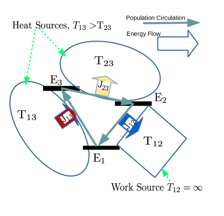
Figure 1: The schematic plot of the three-level heat engine with three system states $E_{j}$, three baths labeled by their temperatures $T_{ij}$ and three energy fluxes $J_{ij}$. The square stands for the work dump and the two ovals for heat baths.

III.1 HEOM for a three-level system

To model the heat engine named above, we need to couple three Caldeira-Leggett baths to the three-level engine Hamiltonian to transit between its levels, the Hamiltonian reads:

$$H=H_{s}+\sum_{ij\in\left\{12,23,13\right\}}\left(H_{b}^{ij}+f_{s}^{ij}g_{b}^{ij}\right).$$ (7)

The system part $H_{s}=\sum_{k=1}^{3}E_{k}\left|k><k\right|$ is simple diagonal with energy levels $E_{k}$. Each bath is a collection of harmonic oscillators $H_{b}^{ij}=\sum_{\alpha}\left[\frac{1}{2}m_{\alpha}^{ij}\left(\omega_{\alpha}^{ij}x_{\alpha}^{ij}\right)^{2}+\frac{\left(p_{\alpha}^{ij}\right)^{2}}{2m_{\alpha}^{ij}}\right]$, where $\alpha$ counts the oscillators of a bath and $ij$ refers to the two system levels exchanged by the said bath. The interaction rises between the collective coordinate of the bath oscillators $g_{b}^{ij}=\sum_{\alpha}c_{\alpha}^{ij}x_{\alpha}^{ij}$ and the transition of the system $f_{s}^{ij}=\left|i><j\right|+c.c.$

The same reasoning as for Eq. (5) leads to the expression of the energy fluxes

$$\left\langle J^{ij}\right\rangle=\frac{i}{\hbar}Tr_{s}\left\{\left[f_{s}^{ij},H_{s}\right]\tilde{\rho}_{s,1}^{ij}\right\},$$ (8)

which directly verifies the energy conservation $\frac{d}{dt}Tr_{s}\left(\tilde{\rho}_{s}H_{s}\right)=\sum_{ij\in\left\{12,23,13\right\}}\left\langle J^{ij}\right\rangle$. $\tilde{\rho}_{s,1}^{ij}$ is defined similar to Eq. (3) as

$$\tilde{\rho}_{s,1}^{ij}=M_{u_{1},u_{2}}\left\{\bar{\rho}_{s}\left(t\right)\bar{g}^{ij}\left(t\right)\right\},$$

where $\bar{g}^{ij}\left(t\right)$ is the random force caused by the heat bath $H_{b}^{ij}$. $\bar{\rho}_{s}\left(t\right)$ is determined by a SDE similar to Eq. (4).

The same manipulation briefed in the previous section transforms the SDE of $\bar{\rho}_{s}$ to HEOM (see Appendix A and Ref. yan2012lasercontrol ). We utilize HYSHE package to solve the coupled differential equations of HEOM. HYSHE is designed with optimized data structure to solve quantum dynamics of small systems coupled to multiple Caldeira-Leggett baths and time-dependent driven forces. Many truncation policies are implemented at ready to accelerate the convergence. We adopt Debye-cutoff $\Omega$-form spectral density function

$$J\left(\omega\right)=\eta\omega\frac{1}{\left[1+\left(\omega/\omega_{c}\right)^{2}\right]}$$ (9)

readily provided in the package for all three baths. As the original program only records the first layer of the hierarchy (i.e. the reduced density matrix), some lines are amended to capture and process the second layer terms for the deduction of energy fluxes. The modification is, generally saying, minimal.

III.2 The parameters of the work dump

The immediate outputs of HYSHE are time-dependent bath-specific energy fluxes. Their typical looks are like Figure 2. In the plot, the unit of temperature is set to be $T_{0}=75\text{K }$ and so the units of energy, time, energy flux and friction are derived, respectively, as $\epsilon_{0}=k_{B}T_{0}=1.035\times 10^{-21}\text{J}$, $\tau_{0}=\frac{\hbar}{\epsilon_{0}}=1.019\times 10^{-13}\text{s}$, $j_{0}=\frac{\epsilon_{0}}{\tau_{0}}=1.016\times 10^{-8}\text{J/s}$ and $\eta_{0}=\epsilon_{0}\tau_{0}=\hbar$. The unit of the friction constant $\eta$ is also $\epsilon_{0}$. We choose the solely occupied ground state of the system to start the propagation. The baths are initially in their factorized equilibrium as required by HEOM. The result of a simulation generally displays plateaux of fluxes quickly reached after a short disturbance caused by initial thermalization. Once the steady state builds up, the three fluxes cancel out. The simulation for Figure 2 takes less than an hour to complete on a single core of Xeon E5 CPU.

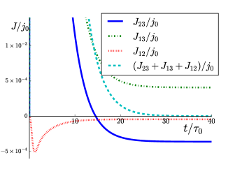
Figure 2: The fluxes $J/j_{0}$ versus the time $t/\tau_{0}$, the parameters for the simulation are $E_{1}/\epsilon_{0}=0$, $E_{2}/\epsilon_{0}=0.1$, $E_{3}/\epsilon_{0}=0.92$, $T_{12}/T_{0}=40$, $T_{23}/T_{0}=3$, $T_{13}/T_{0}=4$, $\eta_{12}/\eta_{0}=0.025$, $\eta_{13}/\eta_{0}=\eta_{23}/\eta_{0}=0.02$ and $\omega_{c}\tau_{0}=2$ for all three baths.

Unlike typical engines working in cycles, the three-level engine works in a steady state. To catch the steady state, the propagation time is chosen sufficiently long to ensure the effect of the initial state fades away. The final (steady) values of the fluxes are then recorded and studied on their relations to the engine parameters.

Now that we have three steady fluxes, the next task is to assign different roles to them by setting up proper parameters to their baths. For a heat engine, two heat sources with relatively higher and lower temperatures are mandatory. The fluxes directed to them balance the entropy ($\frac{\delta E_{1}}{T_{1}}+\frac{\delta E_{2}}{T_{2}}=0$) but leave an energy gap ($\delta E_{1}+\delta E_{2}\neq 0$). The gap should be offset by another work dump bath which takes in proper amount of energy ($\delta E_{3}=-\left(\delta E_{1}+\delta E_{2}\right)$) but no entropy. A mechanic way of setting up such a work dump is to push against a payload. This generally means to introduce a time-dependent HEOM and some interpretations which we will address in the follow-up works. In the present work, we choose the thermodynamic way similar to Ref. allahverdyan2016adaptive to set up the work dump. Simply saying, any energy flowing out of the third bath is accompanied by entropy $\delta S=\frac{\delta E}{T}$. Here $T$ is the temperature of the bath, which also implies the assumption of thermal equilibrium and infinite heat capacity of the bath. It is immediately noticed that setting $T$ to infinity would meet the “energy but no entropy” criteria. In practice the infinitely high temperature can be approximated by a finite but large enough value relative to those of the other two baths. However, as is shown in Figure 3, increasing temperature is not enough by only itself. It depresses the fluxes without a foreseeable non-zero limit while our work-dump bath is expected to have a fixed non-zero limit of flux. The reason is, we hint, that increasing the temperature not only projects the bath to its limiting work-dump behavior, but also moves the targeted limit. To see closer, we first refer to the fact that the effect of the harmonic bath upon our system is completely depicted by the $\Omega$-form spectral density function $J\left(\omega\right)$ and in turn its response function $\alpha\left(t\right)=\frac{1}{\pi}\int_{0}^{\infty}d\omega\ \eta\omega C\left(\omega\right)\left[\coth\left(\frac{\hbar\omega}{2k_{B}T}\right)\cos\left(\omega t\right)-i\sin\left(\omega t\right)\right]$. Here the cutoff function $C\left(\omega\right)$ truncates $J\left(\omega\right)=\eta\omega C\left(\omega\right)$ to finite bandwidth $\omega_{c}$. The limiting work-dump behavior of the bath requires a finite form of $\alpha\left(t\right)$ when temperature $T$ goes to infinity. But exclusively increasing temperature makes an unphysical infinity in the real part of $\alpha\left(t\right)$. To resolve the singularity we observe that the real part of $\alpha\left(t\right)$ depends on $T$ through $\coth\left(\frac{\hbar\omega}{2k_{B}T}\right)$ which converges to $\frac{2k_{B}T}{\hbar\omega}$ when $T$ is large enough. This feature prompts that setting the rest engine parameter $\eta$ proportional to $1/T$ makes the anticipated limit. Without losing generality, we choose units so that $k_{B}=\hbar=1$ and set $\eta=\frac{1}{T}$. For $T\gg\omega_{c}$, the real part of $\alpha\left(t\right)$ is reduced to a finite $\alpha_{R}\left(t\right)=\frac{2}{\pi}\int_{0}^{\infty}d\omega\ C\left(\omega\right)\cos\left(\omega t\right)$. This, along with $\lim_{T\to\infty}\alpha_{I}\left(t\right)=0$, defines the limiting work-dump behavior of the bath. The finite limit of $\alpha\left(t\right)$ promises a non-zero intake of energy and $T\to\infty$ ensures no entropy is attached to the energy. This makes the nature of a work dump. We are aware that the work dump has a characteristic time scale $\omega_{c}^{-1}$. Though there is still not a ubiquitous definition of work consistent throughout all scenarios, it is not surprising that the expected one should be specific upon its time scale. For example, femtosecond time resolution allows one to track the forces and displacements of molecules and estimate the work as their products, while time scale of a second blurs out all details and leaves only heat flux to be observed. To name the same movement work or heat one must specify its time scale beforehand.

In the simulation we take the third bath as the work dump, increase its temperature $T_{12}$ and set $\eta_{12}/\eta_{0}=\frac{1}{T_{12}/T_{0}}$ accordingly while keeping the parameters of the other two baths invariant. The result is displayed in Figure 4. The plateaux in the figure suggest the work-dump limit be reached when $T_{12}$ is much larger than $T_{13}$ and $T_{23}$. In the following simulations we choose $T_{12}$ large enough to safely converge the third bath and study the effect of other parameters.

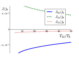
Figure 3: The fluxes $J/j_{0}$ versus the temperature of the work dump $T_{12}/T_{0}$, the parameters set for the simulation are $E_{1}/\epsilon_{0}=0$, $E_{2}/\epsilon_{0}=0.1$, $E_{3}/\epsilon_{0}=0.92$, $T_{23}/T_{0}=3$, $T_{13}/T_{0}=4$, $\eta_{12}/\eta_{0}=0.025$, $\eta_{13}/\eta_{0}=\eta_{23}/\eta_{0}=0.02$ and $\omega_{c}\tau_{0}=2$ for all three baths. $T_{12}/T_{0}$ is increased from $4$ to $50$.

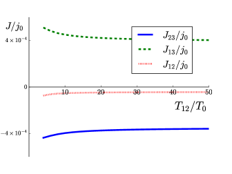
Figure 4: The fluxes $J/j_{0}$ versus the temperature of the work dump $T_{12}/T_{0}$, the parameters set for the simulation are $E_{1}/\epsilon_{0}=0$, $E_{2}/\epsilon_{0}=0.1$, $E_{3}/\epsilon_{0}=0.92$, $T_{23}/T_{0}=3$, $T_{13}/T_{0}=4$, $\eta_{13}/\eta_{0}=\eta_{23}/\eta_{0}=0.02$ and $\omega_{c}\tau_{0}=2$ for all three baths. $T_{12}/T_{0}$ is increased from $4$ to $50$ and $\eta_{12}/\eta_{0}=\frac{1}{\left(T_{12}/T_{0}\right)}$.

IV The efficiency of a three-level heat engine

As an application of the technique proposed above, we study the effect of the parameters on the efficiency of the engine. To isolate the effect, the parameters related to the work dump need to be fixed first, including $T_{12}/T_{0}=40$, $\eta_{12}/\eta_{0}=0.025$, $E_{1}/\epsilon_{0}=0$ and $E_{2}/\epsilon_{0}=0.1$. It leaves us only the parameters of the other two baths and $E_{3}$ to manipulate. We choose to move the only “internal” parameter $E_{3}/\epsilon_{0}$ from $0.2$ to $1.04$ and observe its effect on the efficiency of the engine. The other parameters are set as $T_{13}/T_{0}=4$, $T_{23}/T_{0}=3$ and $\eta_{13}/\eta_{0}=\eta_{23}/\eta_{0}=0.02$. The cutoffs of all three baths are set uniformly as $\omega_{c}\tau_{0}=2.0$. The steady fluxes $J_{12}$, $J_{23}$ and $J_{13}$ are taken from the levels of the plateaux and then fed into the definition $\eta_{eff}=\frac{-J_{12}}{Max\left(J_{13},J_{23}\right)}$(see Ref. allahverdyan2016adaptive ) for the efficiency of the heat engine. For the small coupling strength we choose, the shifts of the energy gaps are negligible, thus the energy flux could be approximated by $I\left(E_{i}-E_{j}\right)$ where $I$ is the population circulation. The efficiency $\eta_{eff}=\frac{I\left(E_{2}-E_{1}\right)}{Max\left(I\left(E_{3}-E_{1}\right),I\left(E_{2}-E_{3}\right)\right)}$ is then found to be independent of the magnitude of $I$. The sign of $I$ is inferred from the sign of the energy flux $J_{ij}$. This theory is compared to the numerical simulation in Figure 5 and the results fit well to each other. Note that the gap in the efficiency $\eta_{eff}$ is caused by the switch from refrigerator to heat engine.

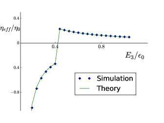
Figure 5: The efficiency of the heat engine $\eta_{eff}/\eta_{0}$ versus $E_{3}/\epsilon_{0}$, the parameters set for the simulation are $E_{1}/\epsilon_{0}=0$, $E_{2}/\epsilon_{0}=0.1$, $T_{12}/T_{0}=40$, $T_{23}/T_{0}=3$, $T_{13}/T_{0}=4$, $\eta_{12}/\eta_{0}=0.025$, $\eta_{13}/\eta_{0}=\eta_{23}/\eta_{0}=0.02$ and $\omega_{c}\tau_{0}=2$ for all three baths. $E_{3}/\epsilon_{0}$ is increased from $0.2$ to $1.04$.

V Conclusion

In the framework of stochastic decoupling and for the bath model comprised of harmonic oscillators, we find the expression of energy flux to be determined by the correlation between the random density matrix of the system and the random force exerted by the bath (Eq. (3) and (5)). Through the connection between stochastic decoupling and HEOM we further express the energy flux as a combination of the terms in the second layer of HEOM. The result makes an efficient and numerically exact approach that calculates energy fluxes accurately. We argue that to convert a bath to a work dump one needs to increase the temperature $T$ of the bath to a large enough value and decrease the friction coefficient $\eta$ accordingly to keep $\eta T$ invariant. With this efficient method we calculate the efficiency of a three-level heat engine weakly coupled to its heat baths. The result compares well to the prediction of a simple theory for weak coupling limit.

Appendix A Energy Fluxes For A Three-Level System

With the help of stochastic decoupling, the SDEs for the system and the baths are shown as, respectively,

$$i\hbar d\rho_{s}\left(t\right)=\left[H_{s},\rho_{s}\left(t\right)\right]dt+\frac{1}{2}\sum_{ij}\left[f_{s}^{ij},\rho_{s}\left(t\right)\right]u_{1,t}^{ij}dt+\frac{i}{2}\sum_{ij}\left\{f_{s}^{ij},\rho_{s}\left(t\right)\right\}u_{2,t}^{ij*}dt$$

$$i\hbar d\rho_{b}^{ij}\left(t\right)=\left[H_{b}^{ij},\rho_{b}^{ij}\left(t\right)\right]dt+\frac{1}{2}\left[g_{b}^{ij},\rho_{b}^{ij}\left(t\right)\right]u_{2,t}^{ij}dt+\frac{i}{2}\left\{g_{b}^{ij},\rho_{b}^{ij}\left(t\right)\right\}u_{1,t}^{ij*}dt.$$

Here $ij\in\Omega=\left\{12,23,13\right\}$. The total density matrix is expressed as the average $\rho\left(t\right)=M\left\{\rho_{s}\prod_{ij\in\Omega}\rho_{b}^{ij}\right\}$. Here the operator $M\left\{\cdot\right\}$ averages its operand over all noises introduced by stochastic decoupling. Applying Itô calculus to the derivative of the average reproduces Liouville equation $i\hbar\frac{d}{dt}\rho=\left[H,\rho\right]$, which demonstrates the validity of the SDEs.

Similar to Eq. (1), the fluxes are defined by the increment of the system energy $\frac{d}{dt}\left\langle H_{s}\right\rangle=-\frac{i}{\hbar}\sum_{ij}\left\langle g_{b}^{ij}\left[H_{s},f_{s}^{ij}\right]\right\rangle=\sum_{r=1}^{3}\left\langle J^{ij}\right\rangle$. With the stochastic expression of $\rho$, the flux $\left\langle J^{ij}\right\rangle=\frac{i}{\hbar}Tr\left\{\rho g_{b}^{ij}\left[f_{s}^{ij},H_{s}\right]\right\}$ is simplified to an expression in the finite-dimensional reduced space

$$\left\langle J^{ij}\right\rangle=\frac{i}{\hbar}Tr_{s}\left\{\left[f_{s}^{ij},H_{s}\right]\tilde{\rho}_{s,1}^{ij}\right\}$$ (10)

where

$$\tilde{\rho}_{s,1}^{ij} =M\left\{\rho_{s}\bar{g}^{ij}\left(t\right)\prod_{i^{{}^{\prime}}j^{{}^{\prime}}\in\Omega}Tr_{b}^{i^{{}^{\prime}}j^{{}^{\prime}}}\left\{\rho_{b}^{i^{{}^{\prime}}j^{{}^{\prime}}}\right\}\right\}$$ (11)

$$\tilde{\rho}_{s,0} =M\left\{\rho_{s}\prod_{i^{{}^{\prime}}j^{{}^{\prime}}\in\Omega}Tr_{b}^{i^{{}^{\prime}}j^{{}^{\prime}}}\left\{\rho_{b}^{i^{{}^{\prime}}j^{{}^{\prime}}}\right\}\right\}.$$ (12)

Here $\bar{g}^{ij}\left(t\right)=\sqrt{\hbar}\int_{0}^{t}\alpha_{I}^{ij}\left(t-\tau\right)u_{2,t^{{}^{\prime}}}^{ij}dt+\sqrt{\hbar}\int_{0}^{t}\alpha_{R}^{ij}\left(t-\tau\right)u_{1,t^{{}^{\prime}}}^{ij*}dt$ is the random force caused by the bath $H_{b}^{ij}$. Girsanov transformation absorbs the trace of the bath density matrices in Eq. (11,12) and reformulates the equations as $\tilde{\rho}_{s,0}=M\left\{\bar{\rho}_{s}\right\}$ and $\tilde{\rho}_{s,1}^{ij}=M\left\{\bar{\rho}_{s}\left(t\right)\bar{g}^{ij}\left(t\right)\right\}$. Here $\bar{\rho}_{s}$ is determined by $i\hbar d\bar{\rho}_{s}=\left[H_{s},\bar{\rho}_{s}\right]dt+\sum_{ij}\left[f_{s}^{ij},\bar{\rho}_{s}\right]\bar{g}^{ij}\left(t\right)dt+\sum_{ij}\left\{\frac{1}{2}\left[f_{s}^{ij},\bar{\rho}_{s}\right]u_{1}^{ij}dt+\frac{i}{2}\left\{f_{s}^{ij},\bar{\rho}_{s}\right\}u_{2}^{ij*}dt\right\}$. Averaging the SDE, we have $i\hbar d\tilde{\rho}_{s}=\left[H_{s},\tilde{\rho}_{s}\right]dt+\sum_{ij}\left[f_{s}^{ij},\rho_{s,1}^{ij}\right]dt$, which easily verifies

$$\frac{d}{dt}Tr_{s}\left(\tilde{\rho}_{s}H_{s}\right)=\sum_{r}\left\langle J^{ij}\right\rangle.$$ (13)

Though in practice HYSHE package itself takes the burden of the job, we would like to bring forward the equations playing behind the codes to add some transparency to the black box. For convenience, we ommit the bath index $ij$ for now. For the chosen spectral density function Eq. (9), the response function is split as:

$$\alpha\left(t\right) =\frac{\eta\omega_{c}^{2}}{2}\left[\cot\left(\beta\hbar\omega_{c}/2\right)-i\right]\exp\left(-\omega_{c}t\right)$$ (14)

$$+\frac{2\eta\omega_{c}^{2}}{\hbar\beta}\sum_{k=1}^{\infty}\frac{v_{k}\exp\left(-v_{k}t\right)}{v_{k}^{2}-\omega_{c}^{2}}$$

here $v_{k}=2\pi k/\left(\hbar\beta\right)$. We denote for clarity the coefficients $C_{0}=\sqrt{\hbar}\frac{\eta\omega_{c}^{2}}{2}\cot\left(\beta\hbar\omega_{c}/2\right)$, $D_{0}=-\sqrt{\hbar}\frac{\eta\omega_{c}^{2}}{2}$ and $\omega_{0}=\omega_{c}$, $C_{J}=\sqrt{\hbar}\frac{2\eta\omega_{c}^{2}}{\hbar\beta}\frac{v_{J}}{v_{J}^{2}-\omega_{c}^{2}}$ and $\omega_{J}=v_{J}$ for $J>0$, thus the response function is split as $\sqrt{\hbar}\alpha\left(t\right)=iD_{0}\exp\left(-\omega_{0}t\right)+\sum_{J=0}^{N}C_{J}\exp\left(-\omega_{J}t\right)$. Respectively $\bar{g}\left(t\right)$ is expressed as

$$\bar{g}\left(t\right) =\sqrt{\hbar}\int_{0}^{t}\alpha_{I}\left(t-\tau\right)u_{2,\tau}d\tau+\sqrt{\hbar}\int_{0}^{t}\alpha_{R}\left(t-\tau\right)u_{1,\tau}^{*}d\tau$$ (15)

$$=\int_{0}^{t}D_{0}\exp\left(-\omega_{0}\left(t-\tau\right)\right)u_{2,\tau}d\tau+\sum_{J=0}^{N}\int_{0}^{t}C_{J}\exp\left(-\omega_{J}\left(t-\tau\right)\right)u_{1,t^{{}^{\prime}}}^{*}d\tau$$

$$=\sum_{J}\bar{g}_{J}\left(t\right)$$

where $\bar{g}_{J}\left(t\right)=\delta_{J,0}\int_{0}^{t}D_{0}\exp\left(-\omega_{0}\left(t-\tau\right)\right)u_{2,\tau}d\tau+\int_{0}^{t}C_{J}\exp\left(-\omega_{J}\left(t-\tau\right)\right)u_{1,\tau}^{*}d\tau$. Its derivative is $d\bar{g}_{J}\left(t\right)=\delta_{J,0}D_{0}u_{2,t}dt+C_{J}u_{1,t}^{*}dt-\left(\delta_{J,0}\omega_{0}\bar{g}_{0,im}\left(t\right)+\omega_{J}\bar{g}_{J,re}\left(t\right)\right)dt$ where $\bar{g}_{0,im}\left(t\right)=\int_{0}^{t}D_{0}\exp\left(-\omega_{0}\left(t-\tau\right)\right)u_{2,\tau}d\tau$, and $\bar{g}_{J,re}\left(t\right)=\int_{0}^{t}C_{J}\exp\left(-\omega_{J}\left(t-\tau\right)\right)u_{1,\tau}^{*}d\tau$.

To avoid confusion the bath index $ij\in\left\{23,13,12\right\}$ will be replaced by $r\in\left\{1,2,3\right\}$ hereafter. In this notation we define $\tilde{\rho}_{I}=M\left\{\bar{\rho}_{s}\prod_{r=1}^{3}\prod_{J=0}^{N}\left(\bar{g}_{J}^{r}\right)^{I_{r,J}}\right\}$, where the subscript $I$ itself is a matrix of non-negative integral entries. Utilizing Itô calculus and averaging over all auxiliary noises we get

$$i\hbar\frac{d}{dt}\tilde{\rho}_{I} =-i\sum_{m=1}^{3}\sum_{n=0}^{N}I_{m,n}\omega_{n}^{m}\tilde{\rho}_{I}+\left[H_{s},\tilde{\rho}_{I}\right]+\sum_{m=1}^{3}\sum_{n=0}^{N}\left[f_{s}^{m},\tilde{\rho}_{I+\Delta_{m,n}}\right]$$ (16)

$$+i\sum_{m=1}^{3}I_{m,0}D_{0}^{m}\left\{f_{s}^{m},\tilde{\rho}_{I-\Delta_{m,0}}\right\}dt+\sum_{m=1}^{3}\sum_{n=0}^{N}I_{m,n}C_{n}^{m}\left[f_{s}^{m},\tilde{\rho}_{I-\Delta_{m,n}}\right].$$

Here $\Delta_{m,n}$ is a matrix defined by its entries $\left(\Delta_{m,n}\right)_{r,J}=\delta_{mr}\delta_{nJ}$. To calculate the energy flux from bath $r$, any term $\rho_{I}$ with all $I$’s entries zero, except one single $1$ at $I$’s $r$’th row, will be summed up to

$$\tilde{\rho}_{s,1}^{r}=\sum_{n}\tilde{\rho}_{\Delta_{r,n}}.$$ (17)

This expression, along with Eq. (10), calculates the energy flux from the $r$’th bath.

In HYSHE proper factors are multiplied to scale the hierarchical terms for better numerical performance:

$$P_{I}=\frac{\prod_{r}\prod_{J=0}^{N}\left(\omega_{J}^{r}\right)^{I_{r,J}}}{\left(\prod_{r}\prod_{J=0}^{N}\left(I_{r,J}!\right)\left|C_{J}^{r}+i\delta_{J0}D_{J}^{r}\right|^{I_{r,J}}\right)^{\frac{1}{2}}}\tilde{\rho}_{I}.$$ (18)

The scaling also changes the hierarchical equations to

$$i\hbar\frac{d}{dt}P_{I} =-i\sum_{m=1}^{3}\sum_{n=0}^{N}I_{m,n}\omega_{n}^{m}P_{I}+\left[H_{s},P_{I}\right]$$ (19)

$$+\sum_{m=1}^{3}\sum_{n=0}^{N}\left(\omega_{n}^{m}\right)^{-1}\left(I_{m,n}+1\right)^{\frac{1}{2}}\left|C_{n}^{m}+i\delta_{n0}D_{0}^{m}\right|^{\frac{1}{2}}\left[f_{s}^{m},P_{I+\Delta_{n,j}}\right]$$

$$+\sum_{m=1}^{3}\sum_{n=1}^{N}\omega_{n}^{m}\left(I_{m,n}\right)^{\frac{1}{2}}\left|C_{n}^{m}\right|^{-\frac{1}{2}}C_{n}^{m}\left[f_{s}^{m},P_{I-\Delta_{m,n}}\right]$$

$$+\omega_{0}^{m}\left|C_{0}^{m}+iD_{0}^{m}\right|^{-\frac{1}{2}}I_{m,0}^{\frac{1}{2}}\sum_{m=1}^{3}\left\{iD_{0}^{m}\left\{f_{s}^{m},P_{I-\Delta_{m,0}}\right\}+C_{0}^{m}\left[f_{s}^{m},P_{I-\Delta_{m,0}}\right]\right\}.$$

Thus to compensate, its raw output of the second layer terms ought to be scaled back to $\tilde{\rho}_{I}=P_{I}\frac{\left(\left|C_{j}^{m}+i\delta_{j0}D_{j}^{m}\right|\right)^{\frac{1}{2}}}{\omega_{J}^{m}}$ before Eq. (17) is employed.

References

• [1] David Gelbwaser-Klimovsky and Alán Aspuru-Guzik. On thermodynamic inconsistencies in several photosynthetic and solar cell models and how to fix them. Chem. Sci., 8(2):1008–1014, January 2017.
• [2] Leo Szilard. On the minimization of entropy in a thermodynamic system with interferences of intelligent beings. Z. Phys., 53:840–856, 1926.
• [3] Richard Feynman. The Feynman Lectures on Physics, volume 1. USA: Addison-Wesley, Massachusetts, 1963.
• [4] Leon Brillouin. Science and Information Theory. Courier Corporation, 2004.
• [5] R. Landauer. Irreversibility and Heat Generation in the Computing Process. IBM J. Res. Dev., 5(3):183–191, July 1961.
• [6] Marcelo O. Magnasco and Gustavo Stolovitzky. Feynman’s Ratchet and Pawl. J. Stat. Phys., 93(3):615–632, November 1998.
• [7] Peter Hänggi and Fabio Marchesoni. Artificial Brownian motors: Controlling transport on the nanoscale. Rev. Mod. Phys., 81(1):387–442, March 2009.
• [8] Yun Zhou and Dvira Segal. Minimal model of a heat engine: Information theory approach. Phys. Rev. E, 82(1):011120, July 2010.
• [9] D. Mandal and C. Jarzynski. Work and information processing in a solvable model of Maxwell’s demon. Proc. Natl. Acad. Sci., 109(29):11641–11645, July 2012.
• [10] H. T. Quan, Yu-Xi Liu, C. P. Sun, and Franco Nori. Quantum thermodynamic cycles and quantum heat engines. Phys. Rev. E, 76(3), September 2007.
• [11] H. E. D. Scovil and E. O. Schulz-DuBois. Three-Level Masers as Heat Engines. Phys. Rev. Lett., 2(6):262–263, March 1959.
• [12] Eitan Geva and Ronnie Kosloff. Three-level quantum amplifier as a heat engine: A study in finite-time thermodynamics. Phys. Rev. E, 49(5):3903–3918, May 1994.
• [13] E. Boukobza and D. J. Tannor. Three-Level Systems as Amplifiers and Attenuators: A Thermodynamic Analysis. Phys. Rev. Lett., 98(24):240601, June 2007.
• [14] A. E. Allahverdyan, S. G. Babajanyan, N. H. Martirosyan, and A. V. Melkikh. Adaptive Heat Engine. Phys. Rev. Lett., 117(3), July 2016.
• [15] G. Lindblad. On the generators of quantum dynamical semigroups. Comm. Math. Phys., 48(2):119–130, June 1976.
• [16] Vittorio Gorini, Andrzej Kossakowski, and E. C. G. Sudarshan. Completely positive dynamical semigroups of N-level systems. J. Math. Phys., 17(5):821–825, May 1976.
• [17] Ronnie Kosloff. A quantum mechanical open system as a model of a heat engine. J. Chem. Phys., 80(4):1625, 1984.
• [18] Ronnie Kosloff. Quantum Thermodynamics: A Dynamical Viewpoint. Comm. Math. Phys., 15(12):2100–2128, May 2013.
• [19] Yoshitaka Tanimura. Nonperturbative expansion method for a quantum system coupled to a harmonic-oscillator bath. Phys. Rev. A, 41(12):6676–6687, June 1990.
• [20] Yun-An Yan, Fan Yang, Yu Liu, and Jiushu Shao. Hierarchical approach based on stochastic decoupling to dissipative systems. Chem. Phys. Lett., 395(4-6):216–221, September 2004.
• [21] Rui-Xue Xu, Ping Cui, Xin-Qi Li, Yan Mo, and YiJing Yan. Exact quantum master equation via the calculus on path integrals. J. Chem. Phys., 122(4):041103, January 2005.
• [22] Qiang Shi, Liping Chen, Guangjun Nan, Rui-Xue Xu, and YiJing Yan. Efficient hierarchical Liouville space propagator to quantum dissipative dynamics. J. Chem. Phys., 130(8):084105, February 2009.
• [23] A.O Caldeira and A.J Leggett. Quantum tunnelling in a dissipative system. Ann. Phys., 149(2):374–456, September 1983.
• [24] Javier Cerrillo, Maximilian Buser, and Tobias Brandes. Nonequilibrium quantum transport coefficients and transient dynamics of full counting statistics in the strong-coupling and non-Markovian regimes. Phys. Rev. B, 94(21):214308, December 2016.
• [25] Jiushu Shao. Decoupling quantum dissipation interaction via stochastic fields. J. Chem. Phys., 120(11):5053–5056, March 2004.
• [26] Yun-An Yan and Oliver Kühn. Laser control of dissipative two-exciton dynamics in molecular aggregates. New J. Phys., 14(10):105004, October 2012.
• [27] A. Ishizaki and G. R. Fleming. Theoretical examination of quantum coherence in a photosynthetic system at physiological temperature. Proc. Natl. Acad. Sci., 106(41):17255–17260, October 2009.
• [28] Liping Chen, Renhui Zheng, Qiang Shi, and YiJing Yan. Two-dimensional electronic spectra from the hierarchical equations of motion method: Application to model dimers. J. Chem. Phys., 132(2):024505, January 2010.
• [29] Jinshuang Jin, Xiao Zheng, and YiJing Yan. Exact dynamics of dissipative electronic systems and quantum transport: Hierarchical equations of motion approach. The Journal of Chemical Physics, 128(23):234703, June 2008.