Capacity allocation through neural network layers

Abstract

Capacity analysis has been recently introduced as a way to analyze how linear models distribute their modelling capacity across the input space. In this paper, we extend the notion of capacity allocation to the case of neural networks with non-linear layers. We show that under some hypotheses the problem is equivalent to linear capacity allocation, within some extended input space that factors in the non-linearities. We introduce the notion of layer decoupling, which quantifies the degree to which a non-linear activation decouples its outputs, and show that it plays a central role in capacity allocation through layers. In the highly non-linear limit where decoupling is total, we show that the propagation of capacity throughout the layers follows a simple markovian rule, which turns into a diffusion PDE in the limit of deep networks with residual layers. This allows us to recover some known results about deep neural networks, such as the size of the effective receptive field, or why ResNets avoid the shattering problem.

1 Introduction

Capacity allocation analysis was recently introduced in [2] as a way to determine quantitatively which dependencies between its inputs and output(s) a trained model has focussed its modelling capacity on. The theory was developed in the context of linear models and $L^{2}$ loss, which corresponds to the Gaussian process prediction task. It was shown that the total model capacity corresponds to the number of independent parameters in the model, and that the capacity allocation could be broken down along any partition of the input space. One partition of particular interest is the spatial partition, i.e. the partition along the canonical dimensions of the input space. This allowed to perform spatial capacity allocation analysis, i.e. to determine which inputs the model has focussed on, and to which degree. This was then used to study two types of 1-dimensional architectures that are commonly used for audio modelling – hierarchical models as in Wavenets [18], and recurrent models [10, 7].

The intuition behind such analysis is to provide tools to peek into the neural black boxes, and understand a posteriori what a given architecture has tried to model, when trained on a given task. Rather than analyzing the network activations as it is often done [17, 20, 16, 21], the idea is to analyze parameters. The extensive quantity thus defined, called the capacity $\kappa$, turns out to have interesting properties. The idea vindicated in [2] is that studying this quantity can lead to new insights on (deep) neural networks, as it is complementary to the value of the loss function: for example, it allows to pinpoint which dependencies the model has tried to capture in order to reduce the value of the loss. When the final goal is more complex than merely minimizing a scalar value, e.g. for content generation tasks, exercising some control over the model’s inductive bias could turn out to be highly valuable, in particular when training full models is long and difficult.

One hypothesis that was put forward in [2] is that the spatial dimension of architecture design (i.e. whether to use recurrent, convolutional, hierarchical models etc.) can be decoupled from its expressivity [13, 12, 5] (i.e. the complexity of the dependencies it can model), and accordingly the analysis was focussed on the spatial aspects in the linear case. Still, when the model takes a linear form in some feature space (obtained e.g. by some non-linear transformation of the inputs), capacity allocation was shown to make sense in that feature space. However, it was suggested that propagating this capacity allocation to the input space is non-trivial in general.

In this paper, we take capacity allocation analysis one step further and investigate the other dimension of the problem by propagating capacity allocation through non-linearities into the input space. More specifically, we analyze the case of neural network layers, which transform their inputs $Y$ according to:

$$\phi(Y)=f(P^{T}Y).$$ (1)

We approach the problem by reducing it to a linear case, by factoring out the non-linearity into some augmented input space. While this requires exponentially large augmented input spaces, we show that two limiting cases are tractable, namely:

1. for linear layers (i.e. when $f$ is the identity function), where one recovers standard capacity allocation in the input space,

2. for pseudo-random layers (in a sense defined below), where the capacity in the input space can be derived explicitly from the capacity in the feature space.

If we introduce the notion of layer decoupling to quantify how much a non-linear activation decouples its outputs, then these two types of layers are two extreme cases of decoupling: linear activations do not modify their inputs and hence perform no decoupling, while pseudo-random activations achieve a full decoupling. On this scale, usual non-linear activations lie somewhere in between, and the extent to which they decouple their outputs is a key element that defines how capacity is transferred from feature space to input space.

The end of this paper focusses on the pseudo-random end of the spectrum, where non-linearity plays a full role (the linear case was already discussed in [2]). We use this framework to analyze deep networks that are made of a large number of such layers, and show that capacity propagation through layers can be described by some linear capacity network, which acts backwards from the output space to the input space, and which can be approximated by a simple diffusion PDE in some scaling limits. This allows us to use the power of PDE analysis to study deep neural networks, and recover in passing some well-known results about the effective receptive field and the shattering problem.

We start by introducing the capacity allocation problem in the case of single neural network layers in Section 2, where we introduce the notions of augmented input space and layer decoupling. We then study two limiting cases: the linear case and the pseudo-random case, where the capacity in the input space can be computed directly from the capacity in the feature space under some independence hypotheses. We then build upon these results to turn to the case of deep networks in Section 3, where we show that in some limit capacity propagation through layers follows a diffusion PDE. We finally leverage these findings in Sections 4 where we address some fundamental questions about the behaviour of deep networks.

2 Capacity allocation of single neural network layers

2.1 The problem

The concept of capacity in a feature space was introduced in [2] and defined as follows. For some function $\phi$ that maps some input $Y\in\mathbb{R}^{n}$ to some intermediate space $\mathbb{R}^{m}$, we consider models of the form $\varphi_{W}(Y)=A_{W}^{T}\phi(Y)$, where the vector of coefficients $A_{W}$ is parametrized by $W\in\mathbb{R}^{p}$. The coefficients space is defined as $\mathcal{A}=\left\{A_{W}\in\mathbb{R}^{m}\mid W\in\mathbb{R}^{p}\right\}$. Since the model is linear in the space of $\phi(Y)$ (a.k.a. the feature space), capacity allocation in that space can be computed by applying linear capacity analysis. The capacity allocated to some subspace $\mathcal{S}^{\phi}$ of the feature space is noted $\kappa^{\phi}(\mathcal{S}^{\phi})$. The next step is then to compute the capacity allocation in the input space, but this question remains unanswered in general. Here we focus on a special class of mapping functions $\phi$, namely single neural network layers that can be written as:

$$\phi(Y)=f(P^{T}Y),$$ (2)

where $P=\{p_{1},...,p_{m}\}\in\mathbb{R}^{n\times m}$ is a linear transformation such that the vectors $p_{i}$ are all distinct, and $f(\cdot)$ is a pointwise non-linear function (such as ReLU, sigmoid, etc.). We assume for simplicity that the $p_{i}$’s are also normalized to $\|p_{i}\|_{2}=1$. The full model therefore reads:

$$\varphi_{W}(Y)=A_{W}^{T}f(P^{T}Y),$$ (3)

We will be mostly interested in how $A_{W}$ allocated its capacity in the input space, assuming that $P$ is constant (which we assume for simplicity, but happens to be a common practice that can give good results [14, 15]). We will briefly consider the case where $P$ is itself learned in Appendix A, and suggest that it might be handled in a similar way – at least in some circumstances.

2.2 Rewriting the problem in the augmented input space

The main idea is to rewrite the non-linear function $f(\cdot)$ from Eq. (3) as:

$$f(z)=\eta_{z}z,$$ (4)

where $\eta_{z}$ is by definition equal to $f(z)/z$. We can then rewrite $\varphi$ as:

$$\varphi(Y) =A^{T}\left(\eta\odot P^{T}Y\right),\quad\eta=(\eta_{1},...,\eta_{m}).$$ (5)

$$: =A^{T}\tilde{P}^{T}\tilde{Y}$$

where $\eta_{i}$ is a shortcut for $\eta_{(P^{T}Y)_{i}}$ and:

$$\tilde{P}=\begin{bmatrix}&p_{1}&0&\ldots&0\\ &0&p_{2}&\ldots&0\\ &\vdots&\vdots&\ddots&\vdots\\ &0&0&\ldots&p_{m}\end{bmatrix}\in\mathbb{R}^{nm\times m},\quad\tilde{Y}=\begin{bmatrix}\eta_{1}y_{1}\\ \vdots\\ \eta_{1}y_{n}\\ \vdots\\ \eta_{m}y_{1}\\ \vdots\\ \eta_{m}y_{n}\\ \end{bmatrix}\in\mathbb{R}^{nm}.$$ (6)

Figure 1: Linearizing a layer by decoupling the paths. The non-linearity $\eta$ is factored in the augmented input space, which allows us to re-write $A^{T}f(P^{T}Y)$ as $A^{T}\tilde{P}^{T}\tilde{Y}$.

What we have done here is simply to decouple the components of $Y$ according to the particular $\eta_{i}$ that multiplies them when going through $f$ (see Figure 1 for an illustration).

Now let us consider the optimal model that satisfies:

$$\varphi^{*}(Y)=\underset{\varphi}{\text{argmin }}\mathbb{E}\left[\left(\varphi(Y)-\varphi_{W}(Y)\right)^{2}\right]:=\mathcal{L}_{W}$$ (7)

which can by definition be written in the form $\varphi^{*}(Y)=A^{*T}\tilde{P}^{*T}\tilde{Y}$. The idea is to use $\varphi^{*}$ as a surrogate “true” process to replace $\varphi_{W}$ in the calculation of the capacity. The $L^{2}$ loss function associated to this process can then be written as:

$$\mathcal{L} =\mathbb{E}\left[\left(\varphi(Y)-\varphi^{*}(Y)\right)^{2}\right]$$ (8)

$$=\left(\tilde{P}A-\tilde{P}^{*}A^{*}\right)^{T}\tilde{\Sigma}\left(\tilde{P}A-\tilde{P}^{*}A^{*}\right)$$

where $\tilde{\Sigma}:=\mathbb{E}(\tilde{Y}\tilde{Y}^{T})$ is the covariance matrix in the augmented input space. Cancelling the derivative of $\mathcal{L}$ with respect to the model parameters gives:

$$\frac{\partial\mathcal{L}}{\partial W}=0 \Leftrightarrow\quad\tilde{K}^{T}\tilde{X}=0,\quad\quad\tilde{K}:=\tilde{\Sigma}\frac{\partial\tilde{P}A}{\partial W}\in\mathbb{R}^{nm\times p}$$ (9)

where $\tilde{K}$ is the capacity matrix in the augmented input space and where we have defined $\tilde{X}:=\left(\tilde{P}A-\tilde{P}^{*}A^{*}\right)$ as the error in the space of the coefficients applied to $\tilde{Y}$. Note that the surrogate process $\varphi^{*}$ does not intervene in the expression of $\tilde{K}$, as expected. We have recovered the exact same equations as in the linear case [2], but applied in the augmented input space (i.e. the space of $\tilde{Y}$).

Note that the above equivalence holds since $\tilde{\Sigma}$ does not depend on the model parameters, which follows from the fact that $\eta$ does not depend on $A$. If $P$ is itself learned, computing its capacity allocated in the input space is trickier as $\eta$ and therefore $\tilde{\Sigma}$ depend on $P$. We however suggest in Appendix A that the above equation might hold in general, or at least in some cases (including the linear case but also piecewise linear functions like ReLU, leaky ReLU or absolute value).

2.3 Layer decoupling

The intuition that underlies the above reformulation of the problem in the augmented input space is that a pointwise (non-linear) function $f$ decouples its outputs from each other. The degree of decoupling however depends on the particular activation $f$ that is used. Below we consider several types of activations and analyze their effects on $\tilde{\Sigma}$.

Linear activations

Choosing $f$ as the identity leads to no decoupling at all:

$$\forall y,~{}\eta_{y}=1\quad\Rightarrow\quad\tilde{\Sigma}=\begin{bmatrix}&\Sigma&\Sigma&\ldots&\Sigma\\ &\Sigma&\Sigma&\ldots&\Sigma\\ &\vdots&\vdots&\ddots&\vdots\\ &\Sigma&\Sigma&\ldots&\Sigma\end{bmatrix}\in\mathbb{R}^{nm\times nm}.$$ (10)

i.e. the original inputs are simply repeated identically $m$ times. The correlation matrix is thus repeated $m$ times in both directions (see Figure 2, left).

Figure 2: (left) For linear layers where $\eta_{1}=\eta_{2}=1$, no decoupling happens and the inputs are merely repeated. In this degenerate case, the capacity in the augmented input space matches the capacity in the original input space. (right) For non-linear layers, the inputs are decoupled by multiplication with the $\eta$’s. In the pseudo-random limiting case, the left (green) and the right (yellow) blocks become independent.

Pseudo-random activations

The other extreme would be an activation function whose outputs are fully decoupled (which we call pseudo-random activations):

$$\mathbb{E}_{z}(\eta_{z})=0,\quad\mathbb{E}_{z_{1},z_{2}}(\eta_{z_{1}}\eta_{z_{2}})=\sigma^{2}\delta_{z_{1}-z_{2}}\quad\Rightarrow\quad\tilde{\Sigma}=\sigma^{2}\begin{bmatrix}&\Sigma&0&\ldots&0\\ &0&\Sigma&\ldots&0\\ &\vdots&\vdots&\ddots&\vdots\\ &0&0&\ldots&\Sigma\end{bmatrix}\in\mathbb{R}^{nm\times nm},$$ (11)

where we will often set $\sigma=1$ for simplicity. We use the terminology “pseudo-random activation” since it corresponds to a non-linear function $f$ that is nowhere continuous, and such that the outputs corresponding to two arbitrarily close inputs can be effectively considered to be independent. In this case, the augmented inputs consist of $m$ independent blocks that are each based upon the $n$ original inputs (see Figure 2, right).

ReLU, Leaky ReLU, Absolute value

More usual non-linear activations like ReLU [11, 4], leaky ReLU [9] (and its variants [19]) or absolute value lead to intermediate $\tilde{\Sigma}$’s, with extra-diagonal matrices that are weaker than $\Sigma$ but stronger than 0. If $\eta$ can be expressed as:

$$\eta(z)=\alpha\mathbbm{1}_{z\leq 0}+\beta\mathbbm{1}_{z>0},$$ (12)

where $\alpha,\beta$ are normalized such that $\alpha^{2}+\beta^{2}=2$, then one can show that if $z_{i}$ and $z_{j}$ are independent random variables that are symmetric around 0, then for any variables $y_{k}$, $y_{l}$ one has:

$$\begin{cases}\mathbb{E}\left[\eta(z_{i})^{2}y_{k}y_{l}\right]=\mathbb{E}\left[y_{k}y_{l}\right],\\ \mathbb{E}\left[\eta(z_{i})\eta(z_{j})y_{k}y_{l}\right]\simeq\nu\mathbb{E}\left[y_{k}y_{l}\right],\end{cases}\quad\text{with }\nu=\frac{1}{4}\left(\alpha+\beta\right)^{2}.$$ (13)

The covariance matrix in the augmented space therefore reads:

$$\tilde{\Sigma}\simeq\begin{bmatrix}&\Sigma&\nu\Sigma&\ldots&\nu\Sigma\\ &\nu\Sigma&\Sigma&\ldots&\nu\Sigma\\ &\vdots&\vdots&\ddots&\vdots\\ &\nu\Sigma&\nu\Sigma&\ldots&\Sigma\end{bmatrix}\in\mathbb{R}^{nm\times nm}.$$ (14)

The linear case $\alpha=\beta=1$ yields $\nu=1$ as expected, while a ReLU non-linearity yields $\nu=\frac{1}{2}$ and an absolute value non-linearity with $\alpha=-1$, $\beta=1$ yields $\nu=0$. The leaky ReLU case $\alpha>0$, $\beta>1$ lies somewhere between the linear case and the ReLU case. One could thus be tempted to introduce a decoupling scale to qualify the position of a non-linear activation between the two extreme types discussed above (see also Figure 3):

$$\underbrace{\text{Linear}}_{\nu=1}<\underbrace{\text{Leaky ReLU}}_{\frac{1}{2}<\nu<1}<\underbrace{\text{ReLU}}_{\nu=\frac{1}{2}}<\underbrace{\text{Abs}}_{\nu=0}<\underbrace{\text{Pseudo-random}}_{\nu=0}$$ (15)

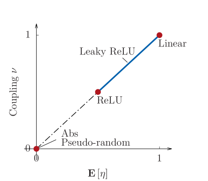
Figure 3: The decoupling scale, from fully coupled blocks for the linear layers ($\nu=\mathbb{E}\left[\eta\right]=1$, top right) to fully decoupled blocks for pseudo-random layers ($\nu=\mathbb{E}\left[\eta\right]=0$, bottom left), with Leaky ReLU and ReLU layers in between.

Note that here the $\nu$’s are given as an indication and correspond to the case where the $y$’s are independent and symmetric around 0.

2.4 Linear activations

If $f$ is taken to be linear, which corresponds to the plain form of $\tilde{\Sigma}$ in Eq. (10) above, it is easy to verify that:

$$\tilde{K}=\frac{1}{\sqrt{m}}\begin{bmatrix}K\\ K\\ ...\\ K\end{bmatrix}$$ (16)

where $K=\Sigma\frac{\partial PA}{\partial W}\in\mathbb{R}^{n\times p}$ is the capacity matrix that would be obtained by the standard method in the space of the original input $Y$. The capacity allocated to a subspace $\mathcal{S}$ of the input space, which reads $\kappa(\mathcal{S})=\|K^{T}S\|_{F}^{2}$ in the input space, can then be computed in the augmented input space as:

$$\tilde{\kappa}(\tilde{\mathcal{S}})=\|\tilde{K}^{T}\tilde{S}\|_{F}^{2},\quad\text{where }\tilde{S}:=\begin{bmatrix}&S&0&\ldots&0\\ &0&S&\ldots&0\\ &\vdots&\vdots&\ddots&\vdots\\ &0&0&\ldots&S\end{bmatrix}.$$ (17)

Indeed, one can then check that this leads to:

$$\tilde{\kappa}(\tilde{\mathcal{S}})=\kappa(\mathcal{S}).$$ (18)

This means that computing the capacity in the augmented input space is equivalent to computing the capacities in the original space – but with more detailed intermediate results. This can therefore be considered as a generalization of the standard method, which we will use below to compute capacities for non-linear activations.

2.5 Pseudo-random activations

Tractable expressions for the capacity can also be obtained at the other end of the spectrum, for what we called pseudo-random activations above. As seen above, this case corresponds to choosing $\eta$ as a realization of some i.i.d. process such that:

$$\mathbb{E}(\eta_{z})=0,\quad\mathbb{E}(\eta_{z_{1}}\eta_{z_{2}})=\delta_{z_{1}-z_{2}}\quad\text{for $z$, $z_{1}$, $z_{2}\in\mathbb{R}$}.$$ (19)

Let us recall the expression of the network output:

$$\varphi(Y)=A^{T}f(P^{T}Y)=A^{T}\tilde{P}^{T}\tilde{Y}.$$ (20)

where only the last layer $A$ is learned. If we decompose the Gram matrix as $\frac{\partial A}{\partial W}\frac{\partial A^{T}}{\partial W}=Q^{\phi}\Lambda Q^{\phi T}$ and note $K^{\phi}$ the columns of $Q^{\phi}$ that correspond to the non-zero eigenvalues, then the optimality criterion on the loss $\mathcal{L}$ can be written as:

$$K^{\phi T}\tilde{P}^{T}\tilde{\Sigma}(\tilde{P}A-\tilde{P}A^{*})=0\quad\Leftrightarrow\quad\left(\tilde{\Sigma}\tilde{P}K^{\phi}\right)^{T}.\tilde{X}=0.$$ (21)

The matrix $\tilde{\Sigma}\tilde{P}K^{\phi}$ does not have orthonormal columns in general, and therefore a further orthonormalization is necessary to obtain the expression of the capacity. However, in the specific case where $\Sigma=\sigma^{2}\mathbb{I}$ (i.e. where the layer inputs are i.i.d.) this simplifies as:

$$\left(\tilde{P}K^{\phi}\right)^{T}.\tilde{X}=0,$$ (22)

and the orthonormality of the columns of $\tilde{P}K^{\phi}$ stems from that of $\tilde{P}$ (which we have assumed in Section 2) and $K^{\phi}$. We can then write the expression for the capacity in the space of the input $\tilde{Y}$ as:

$$\tilde{\kappa}(\tilde{\mathcal{S}})=\|\tilde{K}^{T}\tilde{S}\|_{F}^{2},\quad\tilde{K}:=\tilde{P}K^{\phi}.$$

One can finally define the capacities along the natural dimensions of the input space $\kappa_{1},...,\kappa_{m}$:

$$\kappa_{i}=\|K^{\phi T}\tilde{P}^{T}\tilde{S}_{i}\|_{F}^{2},\quad\tilde{S}_{i}:=\begin{bmatrix}&e_{i}&0&\ldots&0\\ &0&e_{i}&\ldots&0\\ &\vdots&\vdots&\ddots&\vdots\\ &0&0&\ldots&e_{i}\end{bmatrix}\in\mathbb{R}^{nm\times m},$$ (23)

which aggregates the capacities across all $\eta_{j}y_{i}$ for a given $i$, and leads to:

$$\kappa_{i}=\sum_{j=1}^{m}\|K^{\phi T}p_{ij}e_{j}\|_{F}^{2}=\sum_{j=1}^{m}p_{ij}^{2}\kappa^{\phi}_{j},$$ (24)

where the last equality comes from the expression of the capacity in the feature space $\kappa^{\phi}(\mathcal{S}^{\phi})=\|\left(K^{\phi}\right)^{T}S^{\phi}\|_{F}^{2}$. The above expression can be rewritten as:

$$\kappa=D.\kappa^{\phi}$$ (25)

where $D:=P\circ P\in\mathbb{R}^{n\times m}$ is a column-stochastic matrix which preserves the total capacity, and we have defined the spatial capacities along the canonical dimensions of the input and feature spaces, $\kappa=\left(\kappa_{1},...,\kappa_{n}\right)$ and $\kappa^{\phi}=(\kappa^{\phi}_{1},...,\kappa^{\phi}_{m})$. According to this formula, the capacity $\kappa^{\phi}_{j}$ allocated to a given component in the feature space propagates to its associated inputs, according to the corresponding (normalized) square coefficient of $P$. Note that this transformation conserves the total capacity: for $\mathcal{S}=\mathbb{R}^{n}$, one has $\kappa(\mathbb{R}^{n})=\sum_{i=1}^{n}\kappa_{i}=\sum_{i=1}^{m}\kappa_{i}^{\phi}=\kappa^{\phi}(\mathbb{R}^{m})$.

The fact that capacity allocation to a layer inputs only depends on the capacity allocation to the layer outputs is highly interesting. This means that the equation that describes capacity propagation through layers might hold more universally than in the above case where it was derived (namely a $L^{2}$ loss function and a linear last layer): rather, it might well be valid for any feature space capacity $\kappa^{\phi}_{j}$, however derived. We leave this question open for future work.

3 Multiple neural network layers

The capacity propagation equation (25) obtained in the single layer case can be easily generalized in the multi-layer case, as we now show.

3.1 General formula

One can extend the above analysis in the case where $\phi$ is a composition of layers:

$$\phi(Y)=\phi_{L}\circ...\circ\phi_{1}(Y),\quad\text{where}\quad\forall l,~{}\phi_{l}(Y)=f_{l}(P_{l}^{T}Y),$$ (26)

where $f_{l}(\cdot)$ is a pointwise non-linear function and $P_{l}\in\mathbb{R}^{n_{l-1}\times n_{l}}$ is a linear transformation such that $p_{i}$ are all distinct and normalized to $\|p_{i}\|_{2}=1$, as above. Compared with the previous section, we now have $n_{L}\leftrightarrow m$ and $L\leftrightarrow\phi$ at the uppermost layer. From now on, we will focus on the pseudo-random case unless mentioned otherwise. From Eq. (25), one can write the spatial capacities at layer $l-1$ as a function of the spatial capacities at layer $l$:

$$\kappa^{l-1}=D_{l}.\kappa^{l}$$ (27)

where $D_{l}:=P_{l}\circ P_{l}\in\mathbb{R}^{n_{l-1}\times n_{l}}$. By recursion, one finds:

$$\kappa^{0}=D_{1}...D_{L}\kappa^{L}$$ (28)

As mentioned above, the column-stochasticity of the matrices $D_{l}$ results in the conservation of the total capacity, throughout the intermediate feature spaces in the network – and all the way to the input space (see Figure 4 for an illustration).

The remarkable feature of Eq. (28) is that it effectively linearizes the neural network, with the main difference that this network is applied backwards (in layers) to the capacities rather than forwards to the inputs. We call this network the capacity network. Although the results have only been derived under specific hypotheses (essentially, an i.i.d. assumption on the network inputs), this opens the door to analyzing neural networks as linear objects (with the network depth playing the role of time in usual systems), with all the power of linear techniques and a breadth of potential insights. In Section 4, we will consider a few examples where studying capacity allows to recover some well-known and empirical results about deep neural networks – an encouraging start.

Figure 4: Illustration of the backward propagation of capacity through multiple layers. The blue shades indicate how the capacity allocated to the $i$-th node of the last layer (corresponding to a dirac delta $\kappa^{L}$) is propagated all the way through the input layer, resulting in a diffused $\kappa^{0}$. Darker shades corresponds to higher capacity per input. In the deep limit, the propagation is governed by a diffusion PDE, with an effective receptive field that grows as the square root of the number of layers (see Section 4.1).

3.2 Limiting behaviours

A powerful method for analyzing Eq. (28) is to consider the deep limit where:

$$\begin{cases}\forall i,n_{i}=n=m,\\ L=1/\epsilon,\\ D_{1}=...=D_{L}=\mathbb{I}+\epsilon\Delta,\end{cases}$$ (29)

where $\Delta$ is a matrix of order 1 (assumed to be layer-independant for simplicity) and $\epsilon\to 0$. This amounts to considering deep networks with a large number of layers and a “residual” shape for the weights [6] such that each layer only applies a small transformation to its inputs. If we note $\pi(t)=\kappa^{\frac{1-t}{\epsilon}}$, such that $\pi(0)=\kappa^{L}$ and $\pi(1)=\kappa^{0}$, then $\pi$ satisfies the Kolmogorov forward equation [3]:

$$\pi^{\prime}(t)=\Delta\pi(t).$$ (30)

If $\Delta$ is a 1-dimensional local, translation-invariant operator that is non-zero only for $j\in\{i-1,i,i+1\}$, then it can be approximated by the following PDE:

$$\pi^{\prime}(t)=-v\frac{\partial\pi}{\partial x}+\mathcal{D}\frac{\partial^{2}\pi}{\partial x^{2}}.$$ (31)

The solution to this PDE can be written as:

$$\pi(t,x)=\frac{1}{\sqrt{4\pi\mathcal{D}t}}\int_{-\infty}^{\infty}e^{-\frac{(x-y-vt)^{2}}{4\mathcal{D}t}}\pi(0,y)\mathrm{d}y$$ (32)

If the $D_{l}$’s are not all equal but random, by symmetry one should obtain $v=0$ (cf [8]), and therefore we obtain in the space of capacities:

$$\kappa^{l}(x)=\frac{1}{\sqrt{4\pi\mathcal{D}t}}\int_{-\infty}^{\infty}e^{-\frac{(x-y)^{2}}{4\mathcal{D}t}}\kappa^{L}(y)\mathrm{d}y,$$ (33)

where $t=(L-l)/L$.

3.3 Differential layers

Another case that yields the above capacity propagation is the following variant of residual layers, where the non-linear activation is applied to the residual only:

$$\phi_{l}(Y)=Y+\sqrt{\epsilon}f_{l}(P_{l}^{T}Y)$$ (34)

We call this a differential layer, as it learns exactly the difference between its inputs and its outputs. In this case, the neural network itself can be written as a differential equation in the deep limit. If we note $\epsilon=1/L$, $t=l/L$ where $l$ is the layer number and $y(t):=\phi_{l}\circ...\circ\phi_{1}(Y)$, one can rewrite Eq. (34) as:

$$y(t+\epsilon)-y(t)=\sqrt{\epsilon}f_{l}(P^{T}_{t/\epsilon}y),$$ (35)

which is akin to a non-linear forward differential equation applied to the input in the $\epsilon\to 0$ limit (remember a contrario that the capacity PDE is backward in layers). If $P$ is local as in the previous section, then this can be approximated by the following equation in the 1-dimensional case:

$$y(t+\epsilon)-y(t)=\sqrt{\epsilon}f\left(\nu^{Y}_{t}y-v^{Y}_{t}\frac{\partial y}{\partial x}+\mathcal{D}^{Y}_{t}\frac{\partial^{2}y}{\partial x^{2}}\right).$$ (36)

The corresponding capacity PDE in the pseudo-random case is derived in Appendix B, and reads:

$$\pi^{\prime}(t)=2[\mathrm{d}\mathcal{D}^{Y}_{t},\mathrm{d}\mathcal{D}^{Y}_{t}]\frac{\partial^{2}\pi}{\partial x^{2}},$$ (37)

which is similar to the capacity propagation PDE obtained for the type of residual layers studied in the previous section (Eq. 31). The nice additional property in the differential case is that the diffusion coefficient can be linked explicitly to the diffusion coefficient of the SDE that the forward neural network itself implements (Eq. 36).

4 Applications to theoretical analysis of neural networks

Eqs. (28) and (33) for the propagation of capacity allocation through neural network layers open the door to a number of highly interesting analyses, which uncover some established theoretical and empirical facts about (deep) neural networks. In this section we use the capacity framework to study two questions: the size of the effective receptive field of a deep neural network, and the shattering problem [1].

4.1 The effective receptive field of deep networks

The above results show that the spatial capacity $\kappa^{L}$ of the uppermost layer is being spatially diffused as it passes through the layers. For example, if the spatial capacity at the uppermost layer $\kappa^{L}(x)$ takes the form of a Dirac delta $\kappa^{L}(x)=\kappa^{L}\delta_{x-x_{0}}$, then the resulting spatial capacity in intermediate feature spaces is Gaussian:

$$\kappa^{l}(x)=\frac{e^{-\frac{(x-x_{0})^{2}}{4\mathcal{D}t}}}{\sqrt{4\pi\mathcal{D}t}}~{}\kappa^{L},$$ (38)

where $t=(L-l)/L$. The larger $L-l$, i.e. the number of layers traversed, the larger the diffusion region (which one might think of as the effective receptive field – see Figure 4). The size of the diffusion region scales as the square root of the number of layers that are traversed since $L-l~{}\propto~{}t$ (rather than linearly, as one might naively think), and in the amplitude of $\Delta$ (which is $\propto~{}\mathcal{D}$). These results are consistent with the ones of [8], who found such a Gaussian distribution with square root scaling both theoretically in the linear and the random weights cases, and empirically in the general non-linear case. Interestingly, their assumptions and their derivation of the results are very similar to the ones used here – but in the space of gradients rather than capacities. Note that we described the 1-dimensional case here, but such diffusion equation with square root spatial scaling can be derived in arbitrary numbers of dimensions.

4.2 Residual layers and shattered capacity

Interestingly, the limiting behaviour described above is very reminiscent of ResNets [6], where the authors:

1. introduced residual connections such that $D_{l}=\mathbb{I}+\epsilon\Delta_{l}$ becomes a good approximation for each layer,

2. use size 3 convolutions, such that $\Delta$ is a local, translation-invariant operator that is non-zero for $j\in\{i-1,i,i+1\}$ only.

In this setting, a significant local structure remains at $l=0$ (according to Eqs. (33) and (38)) as the capacity is not “shattered” by passing through the layers. If we decompose the influence of $\kappa^{L}$ on the intermediate capacity $\kappa^{l}$ into the different paths:

$$\kappa^{l}_{i_{l}}=\sum_{i_{L}}\kappa^{L}_{i_{L}}\sum_{i_{l+1},...,i_{L-1}}\underbrace{(D_{l+1})_{i_{l}i_{l+1}}(D_{l+1})_{i_{l+1}i_{l+2}}...(D_{L})_{i_{L-1}i_{L}}}_{\text{Weight }w_{i_{l},...,i_{L}}},$$ (39)

then the path with the highest influence is for $i_{l}=i_{l+1}=...=i_{L}(:=i)$ and its weight is

$$w_{\mathrm{max}}^{i}=\prod_{l^{\prime}=l+1}^{L}(D_{l^{\prime}})_{ii}=\prod_{l^{\prime}=l+1}^{L}\left(1+\epsilon(\Delta_{l^{\prime}})_{ii}\right)\simeq e^{\int_{0}^{t}\Delta_{s}^{i}\mathrm{d}s},$$ (40)

where we used the simplified notation $\Delta_{s}^{i}\leftrightarrow(\Delta_{l})_{ii}$ where $s:=(L-l)/l$. Note that $w_{\mathrm{max}}^{i}<1$ since $(\Delta_{l^{\prime}})_{ii}<0$. Therefore, the weight of the most straightforward path between the last layer capacity $\kappa^{L}$ and the intermediate layer capacity $\kappa^{l}$ decays exponentially with the number of layers. In the case above where $L$ scales as $1/\epsilon$, the matrices $\Delta_{l}$ are of order 1 and therefore the largest weight $e^{\int_{0}^{t}\Delta_{s}^{i}\mathrm{d}s}$ is of order 1.

If, on the other hand, $P$ is uniform with receptive field size $r$ (and thus so is $D$), the weights are uniform and equal to $\left(\frac{1}{r}\right)^{L}$ – i.e. they are vanishingly small. This is very reminiscent of the “shattered gradients” analysis of [1], who have shown how ResNets solve the shattered gradients problem by introducing residual connections – again, using similar methods to ours but applied to the gradients rather than the capacities.

5 Conclusion

In this paper, we have built upon the notion of capacity in the feature space introduced in [2], and addressed the case where the mapping function is a neural network layer. We have shown that in this case, the capacity in the input space can be computed under some special hypotheses. We have derived theoretical results for two limiting ends of the spectrum, namely (i) for linear activations (non-decoupling layers) where the original results are exactly recovered, and (ii) for pseudo-random activations (fully decoupling layers) in which the capacity in the input space can be easily computed as a linear transformation of the capacity in the feature space.

When extending the scope to deep neural networks, we have shown that the propagation of capacity through the network layers follows a linear Markov equation in the pseudo-random case, which can be turned into a PDE under appropriate scalings. The remarkable aspect of this result is that it allows to analyze a non-linear neural network in terms of some linear counterpart (the capacity network) which can then be analyzed using powerful linear methods. Although we have only obtained results in special cases and more work is required to understand the regime where the markovian propagation is valid, the fact that it allowed us to recover some theoretical and empirical findings that have been reported in earlier studies is encouraging – and suggests that capacities and gradients may be two sides of the same coin in the pseudo-random case. More generally, the present analysis suggests that the notion of capacity may provide a new vantage point for studying theoretically a number of fundamental questions in deep learning, and provide a more principled and quantitative framework for architecture design.

Appendix A Generalizing the results

Two challenges arise when trying to generalize the above results:

1. For general non-linearities, $\eta$ depends on $Y$. Therefore, the transition from the augmented input space to the original input space is trickier: it is not clear that one can still add the capacities as if the space was separable.

2. When computing the capacity allocated by lower layers (e.g. if $P$ also becomes a variable), the $\eta$’s used for later layers depend on the parameter of the layer considered. Therefore $\tilde{\Sigma}$ does too, which must be taken into account in the calculation of $\frac{\partial\mathcal{L}}{\partial W}$ in Eq. 9.

One possible solution to (ii) is to restrict the scope to locally linear functions $f$, i.e. functions that can be written as:

$$f(y)=\eta_{y}y,\quad\text{with }f^{\prime}(y)=\eta_{y},$$ (41)

where $\eta_{y}$ is piecewise constant. In that case, for any set of inputs $\{Y^{i}\}_{i=1,\ldots,n}$, an infinitesimal perturbation of the network parameters will keep all the $\eta_{y}$’s constant for all $Y_{i}$ if the perturbation $\epsilon$ is small enough. The possible difficulty is that the more inputs $Y$ are being considered, the smaller $\epsilon$: the result might only be valid in some precise limit where the expectation over $Y$ and the derivative w.r.t. $W$ are being taken jointly – rather than taking the expectation first, then computing the derivative, as was done in Eq. (9).

Justifying (i) seems somewhat trickier. One possibility is to accept the current formula as some approximation of the true capacity. Hopefully, the dependence of the various $\eta$’s on the inputs $Y$ is much weaker than the dependence of $Y$ on itself. This is more likely to be true for non-linearities like ReLU, leaky ReLU or absolute value, where $\eta$ is a simple binary function of its inputs.

Some results produced when applying Eqs. (5) and (6) to lower layers are consistent with what one would expect for piecewise linear, homogeneous functions (i.e. ReLU / leaky ReLU / Absolute value etc.). For example, we have checked that the formula allows to retrieve the correct total capacity for a few handpicked hierarchical architectures. In these cases, one expects some parameter redundancy across layers as the scales of successive layers compensate each other – which is exactly what is found. This also suggests that the formulae break down in any other cases (e.g. sigmoid, tanh…), as the equations would find some redundancy when there is in fact none: ReLU-type functions might actually be the only type of functions that allow for the above analysis. This would be consistent with the particular attention that these functions have previously been given in the literature.

Appendix B Capacity PDE for differential layers

Equation (36) shows, maybe trivially, that a deep network with differential layers and pseudo-random weights can be seen as a non-linear SDE applied to its inputs. The expression of the capacity is similar to the case described in Section 3.2, provided one adds variables in the augmented input space corresponding to the un-modified inputs:

$$\varphi(Y)=A^{T}\left(Y+\sqrt{\epsilon}f(P^{T}Y)\right)=A^{T}\tilde{P}^{T}\tilde{Y},$$ (42)

where:

$$\tilde{P}=\begin{bmatrix}&1&0&\ldots&0\\ &0&1&\ldots&0\\ &0&0&\ldots&1\\ &\sqrt{\epsilon}p_{1}&0&\ldots&0\\ &0&\sqrt{\epsilon}p_{2}&\ldots&0\\ &\vdots&\vdots&\ddots&\vdots\\ &0&0&\ldots&\sqrt{\epsilon}p_{n}\end{bmatrix}\in\mathbb{R}^{n(n+1)\times n},\quad\tilde{Y}=\begin{bmatrix}y_{1}\\ \vdots\\ y_{n}\\ \eta_{1}y_{1}\\ \vdots\\ \eta_{1}y_{n}\\ \vdots\\ \eta_{n}y_{1}\\ \vdots\\ \eta_{n}y_{n}\\ \end{bmatrix}\in\mathbb{R}^{n(n+1)}.$$ (43)

In the pseudo-random case, this leads to the following expression of the spatial capacity in the input space, under the same hypotheses as in Section 3.2 (essentially, $\Sigma=\sigma^{2}\mathbb{I}$ and $\|p_{i}\|_{2}=1$):

$$\kappa_{i}=\frac{1}{1+\epsilon}\left(\kappa^{\phi}_{i}+\epsilon\sum_{j=1}^{m}p_{ij}^{2}\kappa^{\phi}_{j}\right)=\kappa^{\phi}_{i}+\frac{\epsilon}{1+\epsilon}\left(\sum_{j=1}^{m}p_{ij}^{2}\kappa^{\phi}_{j}-\kappa^{\phi}_{i}\right)$$ (44)

which gives:

$$\kappa=D\kappa^{\phi},\quad D:=\mathbb{I}+\frac{\epsilon}{1+\epsilon}\Delta\sim\mathbb{I}+\epsilon\Delta$$ (45)

where $\Delta=P\circ P-\mathbb{I}$. This is very reminiscent of the expressions obtained in Section 3.2, and can be treated in a similar way to obtain the capacity PDE:

$$\pi^{\prime}(t)=-v_{t}\frac{\partial\pi}{\partial x}+\mathcal{D}_{t}\frac{\partial^{2}\pi}{\partial x^{2}}.$$ (46)

If $P$ fluctuates randomly from layer to layer, then by symmetry one would have $v_{t}=0$ (as in Section 3.2) so that the above equation can be rewritten as:

$$\pi^{\prime}(t)=\mathcal{D}_{t}\frac{\partial^{2}\pi}{\partial x^{2}}.$$ (47)

From the expression of $\Delta$, one can check that $[\mathrm{d}\mathcal{D}^{Y}_{t},\mathrm{d}\mathcal{D}^{Y}_{t}]=\frac{1}{2}\mathcal{D}_{t}$, where $\mathcal{D}^{Y}_{t}$ is the diffusion coefficient of the stochastic process implemented by the forward neural network (see Eq. (36)).

References

- [1] David Balduzzi, Marcus Frean, Lennox Leary, JP Lewis, Kurt Wan-Duo Ma, and Brian McWilliams. The shattered gradients problem: If resnets are the answer, then what is the question? arXiv preprint arXiv:1702.08591, 2017.
- [2] Jonathan Donier. Capacity allocation analysis of neural networks: Towards principled architecture design. arXiv preprint arxiv:1902.04485, 2019.
- [3] Crispin Gardiner. Stochastic methods, volume 4. springer Berlin, 2009.
- [4] Xavier Glorot, Antoine Bordes, and Yoshua Bengio. Deep sparse rectifier neural networks. In Proceedings of the fourteenth international conference on artificial intelligence and statistics, pages 315–323, 2011.
- [5] William H Guss and Ruslan Salakhutdinov. On characterizing the capacity of neural networks using algebraic topology. arXiv preprint arXiv:1802.04443, 2018.
- [6] Kaiming He, Xiangyu Zhang, Shaoqing Ren, and Jian Sun. Deep residual learning for image recognition. In Proceedings of the IEEE conference on computer vision and pattern recognition, pages 770–778, 2016.
- [7] Nal Kalchbrenner, Erich Elsen, Karen Simonyan, Seb Noury, Norman Casagrande, Edward Lockhart, Florian Stimberg, Aaron van den Oord, Sander Dieleman, and Koray Kavukcuoglu. Efficient neural audio synthesis. arXiv preprint arXiv:1802.08435, 2018.
- [8] Wenjie Luo, Yujia Li, Raquel Urtasun, and Richard Zemel. Understanding the effective receptive field in deep convolutional neural networks. In Advances in neural information processing systems, pages 4898–4906, 2016.
- [9] Andrew L Maas, Awni Y Hannun, and Andrew Y Ng. Rectifier nonlinearities improve neural network acoustic models. In Proc. icml, volume 30, page 3, 2013.
- [10] Soroush Mehri, Kundan Kumar, Ishaan Gulrajani, Rithesh Kumar, Shubham Jain, Jose Sotelo, Aaron Courville, and Yoshua Bengio. Samplernn: An unconditional end-to-end neural audio generation model. arXiv preprint arXiv:1612.07837, 2016.
- [11] Vinod Nair and Geoffrey E Hinton. Rectified linear units improve restricted boltzmann machines. In Proceedings of the 27th international conference on machine learning (ICML-10), pages 807–814, 2010.
- [12] Ben Poole, Subhaneil Lahiri, Maithra Raghu, Jascha Sohl-Dickstein, and Surya Ganguli. Exponential expressivity in deep neural networks through transient chaos. In Advances in neural information processing systems, pages 3360–3368, 2016.
- [13] Maithra Raghu, Ben Poole, Jon Kleinberg, Surya Ganguli, and Jascha Sohl-Dickstein. On the expressive power of deep neural networks. arXiv preprint arXiv:1606.05336, 2016.
- [14] Amir Rosenfeld and John K Tsotsos. Intriguing properties of randomly weighted networks: Generalizing while learning next to nothing. arXiv preprint arXiv:1802.00844, 2018.
- [15] Andrew M Saxe, Pang Wei Koh, Zhenghao Chen, Maneesh Bhand, Bipin Suresh, and Andrew Y Ng. On random weights and unsupervised feature learning. In ICML, pages 1089–1096, 2011.
- [16] Thibault Sellam, Kevin Lin, Ian Yiran Huang, Michelle Yang, Carl Vondrick, and Eugene Wu. Deepbase: Deep inspection of neural networks. arXiv preprint arXiv:1808.04486, 2018.
- [17] Karen Simonyan, Andrea Vedaldi, and Andrew Zisserman. Deep inside convolutional networks: Visualising image classification models and saliency maps. arXiv preprint arXiv:1312.6034, 2013.
- [18] Aäron Van Den Oord, Sander Dieleman, Heiga Zen, Karen Simonyan, Oriol Vinyals, Alex Graves, Nal Kalchbrenner, Andrew W Senior, and Koray Kavukcuoglu. Wavenet: A generative model for raw audio. In SSW, page 125, 2016.
- [19] Bing Xu, Naiyan Wang, Tianqi Chen, and Mu Li. Empirical evaluation of rectified activations in convolutional network. arXiv preprint arXiv:1505.00853, 2015.
- [20] Matthew D Zeiler and Rob Fergus. Visualizing and understanding convolutional networks. In European conference on computer vision, pages 818–833. Springer, 2014.
- [21] Luisa M Zintgraf, Taco S Cohen, Tameem Adel, and Max Welling. Visualizing deep neural network decisions: Prediction difference analysis. arXiv preprint arXiv:1702.04595, 2017.