Roton-induced Bose polaron in the presence of synthetic spin-orbit coupling

Abstract

We theoretically investigate the quasiparticle (polaron) properties of an impurity immersing in a Bose-Einstein condensate with equal Rashba and Dresselhaus spin-orbit coupling at zero temperature. In the presence of spin-orbit coupling, all bosons can condense into a single plane-wave state with finite momentum, and the corresponding excitation spectrum shows an intriguing roton minimum. We find that the polaron properties are strongly modified by this roton minimum, where the ground state of attractive polaron acquires a nonzero momentum and anisotropic effective mass. Across the resonance of the interaction between impurity and atoms, the polaron evolves into a tight-binding dimer. We show that the evolution is not smooth when the roton structure of the condensate becomes apparent, and a first-order phase transition from a phonon-induced polaron to a roton-induced polaron is observed at a critical interaction strength.

A central paradigm of quantum many-body theories is that elementary excitations above a possibly strongly correlated ground state of a quantum system can be approximated by well-defined quasiparticles. In general, the nature and properties of quasiparticles can characterize quantum phases, be predicted by many-body theories and be measured by experiments Wen (2004). Typically, a quantum phase transition between ground states with different types of order manifests itself as qualitative changes in the excitation spectrum, such as the appearance of energy gaps Sachdev (1999). The quasiparticle excitation spectrum determined by spectral functions in many-body theories, therefore, is a fundamental property of any interacting system Damascelli et al. (2003); Stewart et al. (2008). A mobile impurity interacting with a quantum-mechanical medium is one of the most fundamental many-body systems in condensed matter physics Landau and Pekar (1948). In such a system, the impurity is dressed by coupling to the elementary excitations of the medium and forms a polaron (that is a quasiparticle itself). The concept of polaron has been systematically developed Mahan (2000) and provides deep insights into quantum many-body physics.

The great flexibility and extraordinary controllability make ultracold atomic gases an excellent platform to study polaron physics Massignan et al. (2014). Fermi and Bose polarons, where impurity atoms are immersed respectively in a degenerate Fermi gas Schirotzek et al. (2009); Kohstall et al. (2012); Koschorreck et al. (2012); Zhang et al. (2012); Scazza et al. (2017) and a Bose-Einstein condensate (BEC) Hu et al. (2016); Jørgensen et al. (2016), have both been experimentally realized. Ever since then, theoretical studies have been proposed for a wide range of experimentally accessible platforms: Fermi gases Chevy (2006); Lobo et al. (2006); Combescot et al. (2007); Punk et al. (2009); Mathy et al. (2011); Schmidt et al. (2012), Bose condensates Rath and Schmidt (2013); Shashi et al. (2014); Li and Das Sarma (2014), Fermi superfluids Nishida (2015); Yi and Cui (2015), and long-range interacting systems Kain and Ling (2014); Wang et al. (2015); Schmidt et al. (2016); Camargo et al. (2018). In particular, the tunability of interactions between impurities and host atoms via Feshbach resonances has also stimulated a dramatic theoretical improvement, allowing access to the strong-coupling regime at resonance Levinsen et al. (2015) and revealing physics beyond perturbation treatments Astrakharchik and Pitaevskii (2004); Cucchietti and Timmermans (2006); Kalas and Blume (2006). It is now well understood that, even in the strong-coupling regime, the properties of polaron can still be determined by modeling the impurity coupling to only a few medium excitations: the particle-hole excitations in the case of Fermi gases and the phonon excitations in Bose condensates. By increasing the interaction further, Fermi and Bose polarons turn into tightly bound dimers consisting of the impurity and a single atom, via first- and second-order phase transitions, respectively. In all cases, either polarons or dimers stay in a ground state with zero center-of-mass momentum.

In this Letter, we report the existence of an exotic Bose polaron induced by roton excitations, which could emerge in superfluid helium Greytak and Yan (1969), quasi-two-dimensional dipolar BEC Chomaz et al. (2018), and spin-orbit coupled (SOC) BEC Li et al. (2012); Zheng et al. (2013); Ji et al. (2015), all having a roton minimum in their excitation spectrum. Unlike the conventional Bose polaron associated with phonon excitations, the roton-induced Bose polaron features a ground state with finite center-of-mass momentum and anisotropic effective mass, and may also experience a first-order phase transition towards the dimer formation. We propose that this intriguing quasiparticle could be readily observed in a weakly interacting ⁸⁷Rb Bose gas in the presence of synthetic SOC.

To be specific, we focus here on the Raman-laser-induced SOC with equal Rashba and Dresselhaus weight that has recently been successfully engineered in ultracold quantum gases Lin et al. (2011); Wang et al. (2012); Cheuk et al. (2012); Dalibard et al. (2011); Goldman et al. (2014). At zero temperature $T=0$, a weakly interacting BEC with Raman SOC can in principal exhibits three different quantum phases, namely the stripe, plane-wave (PW) and zero-momentum (ZM) phases, depending on the Rabi frequency $\Omega$ of the Raman lasers. While very interesting properties, such as the emergence of density modulations in analogy with supersolids Wang et al. (2010); Ho and Zhang (2011); Li et al. (2012, 2013); Martone et al. (2014); Chen et al. (2018), have been predicted in the stripe phase, its experimentally accessible parameter space is narrow in typical BEC systems such as ⁸⁷Rb. This makes the observation of supersolid stripes very challenging Li et al. (2016, 2011). Here, we consider polarons in the PW and ZM phases. It is in the PW phase that the Bogoliubov spectrum has a local minimum at a finite quasi-momentum, which is attributed as a roton minimum Zheng et al. (2013).

In greater detail, let us write down the Hamiltonian for the Raman SOC BEC with atomic mass $m_{B}$, $\mathcal{H}_{{\rm BEC}}=\mathcal{H}_{0}+\mathcal{V}_{0}$, where ($\hbar=1$ and the volume $V=1$)

$$\mathcal{H}_{0}=\sum_{\mathbf{q}}\left[a_{\mathbf{q}\uparrow}^{\dagger},a_{\mathbf{q}\downarrow}^{\dagger}\right]\left[\frac{\left(\mathbf{q}-k_{{\rm SO}}\mathbf{\hat{e}}_{x}\sigma_{z}\right)^{2}}{2m_{B}}+\frac{\Omega}{2}\sigma_{x}\right]\left[\begin{array}[]{c}a_{\mathbf{q\uparrow}}\\ a_{\mathbf{q}\downarrow}\end{array}\right]$$ (1)

and $\mathcal{V}_{0}=1/2\sum_{\mathbf{q},\mathbf{q^{\prime},}\mathbf{k^{\prime}};\sigma\sigma^{\prime}}g_{\sigma\sigma^{\prime}}a_{\mathbf{q^{\prime}}\sigma}^{\dagger}a_{\mathbf{k^{\prime}-q^{\prime}}\sigma^{\prime}}^{\dagger}a_{\mathbf{k^{\prime}-q}\sigma^{\prime}}a_{\mathbf{q}\sigma}$. Here, $a_{\mathbf{q}\sigma}^{\dagger}$ ($a_{\mathbf{q}\sigma}$) are creation (annihilation) operators of a boson with spin component $\sigma=\{\uparrow,\downarrow\}$ and momentum $\mathbf{q}$, $k_{{\rm SO}}$ is the SOC strength defined by the recoil energy $E_{{\rm SO}}=k_{{\rm SO}}^{2}/(2m_{B})$, and $\sigma_{x}$ and $\sigma_{z}$ are Pauli matrices. For ⁸⁷Rb, we take the SU(2)-invariant interaction $g_{\sigma\sigma^{\prime}}=g_{B}\equiv 4\pi a_{B}/m_{B}$, $\text{$\forall\sigma$,$\sigma$'}\in\{\uparrow,\downarrow\}$, where $a_{B}$ is the BEC scattering length satisfying $0<a_{B}n^{-1/3}\ll 1$ with $n$ being the BEC density.

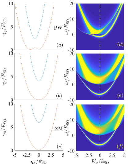
Figure 1: Left panels: Bogoliubov spectrum of a SOC BEC at $\Omega/E_{{\rm SO}}=2,\ 4,\ 6$, with $g_{B}n=0.5E_{{\rm SO}}$ fixed. The two curves in each subplot show the two branches of excitations. Right panels: The corresponding spectral function for an impurity interacting with the BEC with $a_{\uparrow}=0$ and $a_{\downarrow}\rightarrow\infty$. The white dashed lines at $K_{x}=0$ emphasize the asymmetry of the spectrum. Here and in all the following plots, $\delta$-peaks are given a small artificial width to be visible on the graph.

The mean-field ground state can be found via an ansatz that replaces operators $a_{\mathbf{q}\sigma}^{\dagger}$ and $a_{\mathbf{q}\sigma}$ by complex numbers if and only if $\mathbf{q}=\mathbf{p}_{0}$, i.e., $a_{\mathbf{p}_{0}\uparrow}^{\dagger}=a_{\mathbf{p}_{0}\uparrow}=\phi_{\uparrow}\equiv\sqrt{n}\cos\theta$ and $a_{\mathbf{p}_{0}\downarrow}^{\dagger}=a_{\mathbf{p}_{0}\downarrow}=\phi_{\downarrow}\equiv-\sqrt{n}\sin\theta$ Zheng et al. (2013). Minimizing the total energy with respect to variational parameters $\mathbf{p}_{0}$ and $\theta$ determines the ground-state condensate wave function $\left[\phi_{\uparrow},\phi_{\downarrow}\right]$ and BEC chemical potential $\mu_{B}$ for a given $\Omega$. Two different phases are separated by a critical Rabi frequency $\Omega_{c}=4E_{\textrm{SO}}$ Zheng et al. (2013): the PW phase for $\Omega<\Omega_{c}$ where $\theta=0.5\sin^{-1}(\Omega/\Omega_{c})$ and $\mathbf{p}_{0}=k_{{\rm SO}}\cos 2\theta\hat{\mathbf{e}}_{x}$; and the ZM phase for $\Omega\geq\Omega_{c}$ where $\theta=\pi/4$ and $\mathbf{p}_{0}=\mathbf{0}$. These two phases have distinctive quasiparticle spectra $\gamma_{\mathbf{q}}^{(b)}$ as shown in Fig. 1(a)-(c) for the chosen parameters $n=k_{{\rm SO}}^{3}$ and $g_{B}n=0.5E_{\textrm{SO}}$, all of which have upper and lower branches denoted by the superscripts $b=\{+,-\}$, respectively. The polaron properties at low energy are mainly determined by the lower branch. As mentioned earlier, in the PW phase the lower branch of Bogoliubov spectra exhibits a roton minimum near $\mathbf{p_{r}}=p_{r}\hat{\mathbf{e}}_{x}$, as shown in Fig. 1(a). The spectra are calculated by applying Bogoliubov transformations $a_{\mathbf{\mathbf{p}_{0}+q,\sigma}}^{\dagger}=\sum_{b}[u_{\mathbf{q}\sigma}^{(b)}\beta_{\mathbf{q}}^{(b)\dagger}-v_{\mathbf{-q}\sigma}^{(b)}\beta_{-\mathbf{q}}^{(b)}]$ and $a_{\mathbf{p}_{0}-\mathbf{q,\sigma}}=\sum_{b}[u_{\mathbf{-q}\sigma}^{(b)}\beta_{\mathbf{-q}}^{(b)}-v_{\mathbf{q}\sigma}^{(b)}\beta_{\mathbf{q}}^{(b)\dagger}$] with $\beta_{\mathbf{q}}^{(b)\dagger}$ and $\beta_{\mathbf{q}}^{(b)}$ being the creation and annihilation operators of a Bogoliubov excitation. Following Ref. Zhang et al. (2012); Chen et al. (2017), we numerically solve the Bogoliubov parameters $u_{\mathbf{q}\sigma}^{(b)}$, $v_{\mathbf{q}\sigma}^{(b)}$ and spectra $\gamma_{\mathbf{q}}^{(b)}$, to construct the 11-component of the Green function,

$$\left[G_{B}^{(11)}(\mathbf{q},i\nu_{n})\right]_{\sigma\sigma^{\prime}}=\sum_{b}\left[\frac{u_{\mathbf{q}\sigma}^{(b)}u_{\mathbf{q}\sigma^{\prime}}^{(b)}}{i\nu_{n}-\gamma_{\mathbf{q}}^{(b)}}-\frac{v_{\mathbf{-q}\sigma}^{(b)}v_{\mathbf{-q}\sigma^{\prime}}^{(b)}}{i\nu_{n}+\gamma_{\mathbf{-q}}^{(b)}}\right],$$ (2)

where $\nu_{n}=2n\pi k_{B}T$ are bosonic Matsubara frequencies.

By adding an impurity with mass $m_{I}$, the total model Hamiltonian then becomes, $\mathcal{H}=\mathcal{H}_{{\rm BEC}}+\mathcal{H}_{I}+\mathcal{V}_{{\rm int}}$. Here, the impurity Hamiltonian is simply $H_{I}=(\epsilon_{\mathbf{k}}-\mu_{I})c_{\mathbf{k}}^{\dagger}c_{\mathbf{k}}$, where $\mu_{I}$ is the impurity chemical potential, $\epsilon_{\mathbf{k}}=k^{2}/(2m_{I})$ and $c_{\mathbf{k}}^{\dagger}\ (c_{\mathbf{k}})$ is the creation (annihilation) operator of impurity. The interaction between impurity and atoms is described by $\mathcal{V}_{{\rm int}}=\sum_{\sigma}g_{\sigma}^{(I)}\sum_{\mathbf{q},\mathbf{k},\mathbf{k^{\prime}}}a_{\mathbf{k}\sigma}^{\dagger}c_{\mathbf{q}-\mathbf{k}}^{\dagger}c_{\mathbf{q}-\mathbf{k^{\prime}}}a_{\mathbf{k^{\prime}}\sigma},$ where the coupling constants $g_{\sigma}^{(I)}$ are regularized in terms of the impurity-atom scattering lengths $a_{\sigma}$ and reduced mass $\mu_{{\rm IB}}=m_{I}m_{B}/(m_{I}+m_{B})$: $[g_{\sigma}^{(I)}]^{-1}=\mu_{{\rm IB}}/2\pi a_{\sigma}-\sum_{\mathbf{k}}2\mu_{{\rm IB}}/k^{2}$, so that strongly-interacting regime beyond perturbation regime can be accessed. From now on, we focus on the case with $m_{I}=m_{B}=m_{0}$, $a_{\uparrow}=0$ and $a_{\downarrow}\neq 0$.

Without loss of generality, we assume that the impurity is fermionic, and the bare impurity thermal Green function is given by $G_{I}^{(0)}(\mathbf{K},i\Omega_{m})=1/\left[i\Omega_{m}-(\epsilon_{\mathbf{K}}-\mu_{I})\right]$, where $\Omega_{m}=(2m+1)\pi k_{B}T$ are fermionic Matsubara frequencies and $\mathbf{K}$ denotes the center-of-mass momentum. We aim to calculate the full Green’s function incorporating the interaction with BEC

$$G_{I}\left(\mathbf{K},i\Omega_{m}\right)=\frac{1}{i\Omega_{m}-\left(\epsilon_{\mathbf{K}}-\mu_{I}\right)-\Sigma_{I}\left(\mathbf{K},i\Omega_{m}\right)}$$ (3)

that determines the spectral function $A(\mathbf{K},\omega)=-2\Im[G_{I}(\mathbf{K},i\Omega_{m}\rightarrow\omega+i0^{+}-\mu_{I})]$. Here, for a weakly interacting BEC, $\Sigma_{I}(\mathbf{K},i\Omega_{m})\approx\operatorname{Tr}[n_{\mathbf{p}_{0}}\Gamma(\mathbf{K},i\Omega_{m})]$ is the self-energy, and $n_{\mathbf{p}_{0}}$ is a $2\times 2$ matrix with matrix elements $(n_{\mathbf{p}_{0}})_{\sigma\sigma^{\prime}}=\phi_{\sigma}\phi_{\sigma^{\prime}}$. The vertex function is given by $\Gamma(\mathbf{K},i\Omega_{m})^{-1}=g_{I}^{-1}+\chi(\mathbf{K},i\Omega_{m})$, where $g_{I}$ is a diagonal matrix with elements $g_{\sigma}^{(I)}$, and the pair propagator $\chi(\mathbf{K},i\Omega_{m})=k_{B}T\sum_{\mathbf{\mathbf{q}},i\nu_{n}}G_{B}^{(11)}(\mathbf{q},i\nu_{n})G_{I}^{(0)}(\mathbf{K-\mathbf{q}},i\Omega_{m}-i\nu_{n})$. The explicit expressions for the pair propagator $\chi(\mathbf{K},i\Omega_{m})$ and vertex function $\Gamma(\mathbf{K},i\Omega_{m})^{-1}$ as well as the details of derivations are given in Supplemental Material Sup .

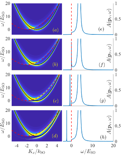
Figure 2: The spectral function for impurity atoms interacting with a SOC BEC at the Rabi frequency $\Omega=E_{{\rm SO}}$. From top to bottom, the parameters are chosen to be $1/(k_{{\rm SO}}a_{\downarrow})=-1,\ 0,\ 0.5,\ 1$, with $a_{\uparrow}=0$ and $g_{B}n=0.5E_{{\rm SO}}$ fixed. Left panels: The frequency and momentum dependency of the spectral function. The red dashed curve shows the dispersion of the center-of-mass of a dimer consisting of a roton and an impurity, and the black solid curve shows the dispersion of a free impurity atom $K_{x}^{2}/(2m_{0})$. Right panels: The spectral function at roton minimum $\mathbf{p}_{r}=p_{r}\hat{\mathbf{e}}_{x}$ as a function of $\omega$. The red dashed line marks the roton minimum energy $\Delta_{r}$.

The frequency and ($K_{x}$, the $x$-component) momentum dependence of the spectral functions are shown in Fig. 1(d)-(f) for $\Omega=2E_{{\rm SO}}$ (PW), $4E_{{\rm SO}}$ (critical) and $6E_{{\rm SO}}$ (ZM) respectively. The spectral function splits into two branches (similar to the polaron spectrum in a conventional BEC). The upper (lower) branch is called a repulsive (attractive) polaron. The repulsive polaron corresponds to a resonance with broad width at high energy. In contrast, the attractive polaron is a well-defined quasiparticle at small momentum and the corresponding spectral function is proportional to a delta function (On the graph, for visibility this $\delta$-peak is given a small artificial width). One can observe that, the polaron spectrum is not symmetric (with respect to $K_{x}\rightarrow-K_{x}$) even in the ZM phase where $\gamma_{\mathbf{q}}^{(b)}$ are symmetric. This can be understood by realizing that $u_{\mathbf{q}}^{(b)}$ and $v_{\mathbf{q}}^{(b)}$ are not symmetric, and the impurity is only interacting with the spin-down component for our choosing parameters ($a_{\uparrow}=0$). This asymmetry of polaron spectrum leads to a minimum of the attractive polaron energy at a non-zero momentum. In another word, the ground state of Bose polaron in the presence of SOC acquires a finite momentum $\mathbf{K}^{*}=K_{x}^{*}\hat{\mathbf{e}}_{x}$. At resonance $a_{\downarrow}\rightarrow\infty$, $\mathbf{K^{*}}$ is much smaller than the roton minimum momentum $\mathbf{p_{r}}$, implying the formation of the polaron ground state is mostly contributed by phonons (the linear dispersion of Bogoliubov spectrum near origin) instead of rotons (the local minimum near $\mathbf{p_{r}}$). Nevertheless, Fig. 1(a) shows that the spectral function has a rich and interesting structure near $\mathbf{p_{r}}$, indicating that the roton minimum in the PW phase strongly modifies the excitation spectrum of polaron at resonance.

To understand the role of rotons better, it is instructive to see how the quasiparticle properties of the polaron changes as the impurity-BEC interaction $a_{\downarrow}$ is varied. As $a_{\downarrow}$ varies across the resonance, an attractive Bose polaron evolves to a tight-binding dimer. Intuitively, if the roton minimum is close enough to zero, we expect that the dimer could be strongly affected by the roton minimum and the polaron spectrum might also be strongly modified. This evolution is shown in Fig. 2 for polarons in the deep PW phase at $\Omega=E_{{\rm SO}}$. For this Rabi frequency, the lower branch of BEC Bogoliubov dispersion $\gamma_{q}^{(-)}$ near the roton minimum along $\hat{x}$ can be approximated by $\gamma_{q}^{(-)}\approx(q_{x}-p_{r})^{2}/m_{x}^{(r)}+\Delta_{r}$, where $p_{r}\approx-1.947k_{{\rm SO}}$, $\Delta_{r}\approx 0.025E_{{\rm SO}}$ and $m_{x}^{(r)}=1.041m_{0}$ can be obtained by numerical fitting. In Fig. 2, we set $(k_{{\rm SO}}a_{\downarrow})^{-1}=-1,\ 0,\ 0.5$ and $1$ from top to bottom. The left panels show the frequency and momentum dependency of spectral functions. The polaron can be understood as a modification of free impurity by dressing medium excitations at perturbation region, and hence the spectral function shows only a single branch of resonances near free-particle dispersions indicated by the black solid curve in Fig. 2(a). We also find that this spectral function acquires a sizable width in regimes above a red dashed threshold curve corresponding to the dispersion of the center-of-mass of a dimer consisting of a roton and an impurity, which along the $x$-axis is given by $(K_{x}-p_{r})^{2}/2[m_{I}+m_{x}^{(r)}]+\Delta_{r}$. Above this threshold, the polaron scatters off virtual roton-impurity dimers and suffers a finite lifetime. At the unitarity $a_{\downarrow}\rightarrow\infty$, sharp peaks show up near the roton-impurity dimer center-of-mass dispersions in Fig. 2(b), and forms an “avoid-cross” at positive intermediate interaction $a_{\downarrow}^{-1}=0.5k_{{\rm SO}}$ in Fig. 2(c). At $a_{\downarrow}^{-1}=k_{{\rm SO}}$ in Fig. 2(d), the polaron spectrum become two well separated branches. These behaviors are emphasized in Fig. 2(e)-(h) for the spectral function at roton minimum momentum $K_{x}=q_{r}\hat{\mathbf{e}}_{x}$. Another peculiar feature for the attractive polaron (lower branches) is the formation of a double-well structure in Fig. 2(c), suggesting that a first-order phase transition is possible in the deep PW phase regime when the Rabi frequency is smaller than a threshold $\Omega^{*}$. Our numerical indicates that $\Omega^{*}=1.2E_{{\rm SO}}$ for our choosing parameters.

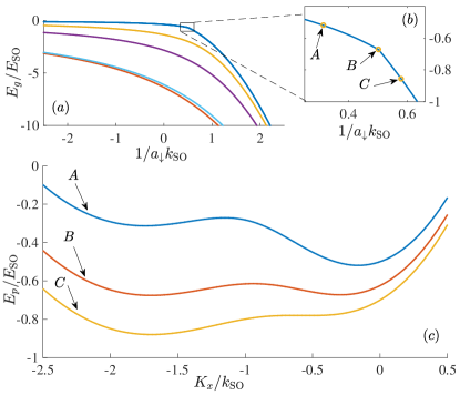
Figure 3: (a) Attractive polaron ground state energy $E_{g}$ as a function of $1/a_{\downarrow}$ at different Rabi frequency $\Omega/E_{{\rm SO}}=1,2,3,4$ and $6$ from top to bottom. We fixed the parameter $a_{\uparrow}=0$ and $g_{B}n=0.5E_{{\rm SO}}$ here. (b) A zoom-in for polaron energy $\Omega=E_{{\rm SO}}$ to emphasize the phase transition. (c) The double minimum structure of attractive polaron energy $E_{p}(K_{x}\hat{\mathbf{e}}_{x})$ as a function of $K_{x}$ at point $A,B$ and $C$ in (b).

The double minimum for attractive polaron at $\Omega=E_{{\rm SO}}$ can be studied qualitatively by examining the polaron energy spectrum given as the pole of the Green function Eq. (3), i.e., $E_{p}(\mathbf{K})\approx\epsilon_{\mathbf{K}}+\operatorname{Tr}[n_{\mathbf{p}_{0}}\Gamma(\mathbf{K},E_{p}(\mathbf{K})-\mu_{I}+i0^{+})]$. We define the attractive polaron ground-state energy $E_{g}$ as the global minimum of $E_{p}(\mathbf{K})$ at momentum $\mathbf{K^{*}}=K_{x}^{*}\hat{\mathbf{e}}_{x}$. In Fig. 3(c), one can clearly see the global minimum change from the one near the origin (that we called phonon-induced polaron) to the one near $p_{r}$ (roton-induced polaron). The polaron energy $E_{g}$ is not smooth as a function of $1/a_{\downarrow}$ at the point $B$ in Fig. 3(b), indicating a first-order phase transition between the phonon-induced and roton-induced polaron. This is in comparison with polaron energy for higher $\Omega>\Omega^{*}$ in Fig. 3(a), which are continuous and smooth.

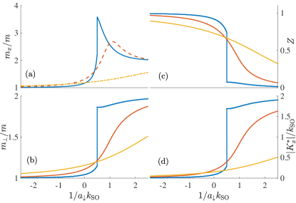
Figure 4: (a) Effective mass $m_{x}$, (b) $m_{\perp}$ (c) spectral residue $Z$ and (d) the center-of-mass momentum $K_{x}^{*}$ of attractive polaron, as a function of $1/a_{\downarrow}$ at different Rabi frequency $\Omega/E_{{\rm SO}}=1,2$ and 6, indicated by blue solid, red dashed and yellow dash-dotted curves correspondingly.

We now address other polaron properties near the global minimum $\mathbf{K^{*}}$ by approximating the Green function near the pole $E_{p}(\mathbf{K}^{*})$ to Rath and Schmidt (2013)

$$G_{I}(\mathbf{K},\omega-\mu_{I})\approx\frac{Z}{\omega-E_{p}(\mathbf{K}^{*})-\frac{\hbar^{2}\left(K_{x}-K_{x}^{*}\right)^{2}}{2m_{x}}-\frac{\hbar^{2}K_{\perp}^{2}}{2m_{\perp}}},$$ (4)

where $Z^{-1}=1-\partial_{\Omega}\left.\sum_{I}(\mathbf{K},\Omega)\right|_{\mathbf{K\rightarrow\mathbf{K^{*}}},\Omega\rightarrow E_{p}(\mathbf{K^{*}})-\mu_{I}}$ is the spectral residue. The effective mass in $x$-direction $m_{x}$ and the perpendicular direction $m_{\perp}$ are given by $Z^{-1}m_{i}^{-1}=m_{0}^{-1}+\left.\partial^{2}\Sigma_{I}\left(\mathbf{K},\Omega\right)/\partial K_{i}^{2}\right|_{\mathbf{K\rightarrow K^{*},}\Omega\rightarrow E_{p}(\mathbf{K^{*}})-\mu_{I}}$, and are in general anisotropic, $m_{x}\neq m_{\perp}$, as shown in Fig. 4(a) and (b) for $\Omega/E_{{\rm SO}}=1,2$ and 6. We also present the spectral residue $Z$ and center-of-mass momentum $K_{x}^{*}$ in Fig. 4(c) and (d). All these quantities show discontinuity for the case $\Omega=E_{{\rm SO}}$, as a result of the first-order transition between roton-induced polaron and dimer. For $\Omega=2E_{{\rm SO}}$ and $6E_{{\rm SO}}$, instead, they change rather smoothly, following the conventional second-order transition from a phonon-induced polaron to a dimer Rath and Schmidt (2013). The first-order transition found here could be related to the parabolic dispersion of the roton. A similar first-order transition is also observed for Fermi polarons, where the dispersion of medium excitations (i.e., particle-hole excitations) is parabolic. In contrast, the phonon dispersion is linear, leading to a smooth polaron-dimer transition for phonon-induced Bose polarons.

In Fig. 4(a), the effective mass $m_{x}$ shows a bump near $1/a_{\downarrow}\approx k_{{\rm SO}}$ at $\Omega=2E_{{\rm SO}}$. This strong deviation of $m_{x}$ from $2m$ shows that the polaron is a genuine many-body effect. Nevertheless, our numerical calculation indicates that this bump become gradually less significant and disappear for larger $\Omega$ but before $\Omega_{c}$ (not shown here), suggesting that the existence of the bump is not a good indicator of the PW phase of the host medium BEC.

The polaron phenomena studied here is experimentally accessible. We may consider a ⁸⁷Rb condensate with scattering length $a_{B}=100a_{0}$. For a laser-induced SOC, the typical SOC strength is set to be $k_{{\rm SO}}=2\pi\times 10^{6}$ m^-1. Our chosen parameter $gn=0.5E_{{\rm SO}}$ then corresponds to a BEC density $n\simeq 3\times 10^{14}$ cm^-3. The impurity can be a ⁸⁷Rb atom in another hyperfine state that is not coupled by the SOC lasers, and the interaction between the impurity and the SOC BEC can be easily tuned by using Feshbach resonances.

In summary, we have predicted the emergence of an exotic quasiparticle - roton-induced Bose polaron - in a spin-orbit coupled Bose-Einstein condensate, which has a nonzero center-of-mass momentum and anisotropic effective masses, and undergoes a first-order polaron-molecule transition upon varying impurity-atom interaction. These unusual properties may also be examined in dipolar Bose condensate and superfluid helium, when rotons are thermally excited at finite temperature.

We are grateful to Professor Zeng-Qiang Yu and Brendan C. Mulkerin for useful discussions. This research was supported by the Australian Research Council (ARC) Discovery Programs, Grants No. DE180100592 and No. DP190100815 (J.W.), No. FT140100003 and No. DP180102018 (X.-J.L), and No. DP170104008 (H.H.).

I Many-body $T$-matrix theory of Bose polarons

Here we generalize the many-body $T$-matrix theory of Bose polarons in Ref. Rath and Schmidt (2013) to a spin-orbit coupled Bose-Einstein condensate (BEC). We have also performed numerical calculations by using Chevy’s variational approach Chevy (2006); Li and Das Sarma (2014), which yields essentially the same results.

I.1 BEC Green function

We construct the zero-temperature Green function of the BEC atoms by using the Bogoliubov parameters $u_{\mathbf{q}\sigma}^{(b)}$, $v_{\mathbf{q}\sigma}^{(b)}$ and Bogoliubov spectra $\gamma_{\mathbf{q}}^{(b)}$,

$$\mathbf{G}_{B}(\mathbf{q},i\nu_{n})=\left[\begin{array}[]{cc}G_{B}^{(11)}(\mathbf{q},i\nu_{n})&G_{B}^{(12)}(\mathbf{q},i\nu_{n})\\ G_{B}^{(21)}(\mathbf{q},i\nu_{n})&G_{B}^{(22)}(\mathbf{q},i\nu_{n})\end{array}\right],$$ (5)

where $G_{B}^{(ij)}$ are two-by-two matrices, whose matrix elements can be explicitly written out as ($\sigma,\sigma^{\prime}=\uparrow,\downarrow$) Zheng et al. (2013),

$$\left[G_{B}^{(11)}(\mathbf{q},i\nu_{n})\right]_{\sigma\sigma^{\prime}}=\left[G_{B}^{(22)}(\mathbf{-q},-i\nu_{n})\right]_{\sigma\sigma^{\prime}}=\sum_{b}\left[\frac{u_{\mathbf{q}\sigma}^{(b)}u_{\mathbf{q}\sigma^{\prime}}^{(b)}}{i\nu_{n}-\gamma_{\mathbf{q}}^{(b)}}-\frac{v_{\mathbf{-q}\sigma}^{(b)}v_{\mathbf{-q}\sigma^{\prime}}^{(b)}}{i\nu_{n}+\gamma_{\mathbf{-q}}^{(b)}}\right],$$ (6)

$$\left[G_{B}^{(12)}(\mathbf{q},i\nu_{n})\right]_{\sigma\sigma^{\prime}}=\left[G_{B}^{(21)}(-\mathbf{q},-i\nu_{n})\right]_{\sigma\sigma^{\prime}}=\sum_{b}\left[-\frac{u_{\mathbf{q}\sigma}^{(b)}v_{\mathbf{q}\sigma^{\prime}}^{(b)}}{i\nu_{n}-\gamma_{\mathbf{q}}^{(b)}}+\frac{v_{\mathbf{-q}\sigma}^{(b)}u_{\mathbf{-q}\sigma^{\prime}}^{(b)}}{i\nu_{n}+\gamma_{\mathbf{-q}}^{(b)}}\right].$$ (7)

where $\nu_{n}=2n\pi k_{B}T$ are bosonic Matsubara frequencies. As shown below, in our diagrammatic treatment within ladder approximation, only the 11-component of the propagator $G_{B}^{(11)}$ is needed to calculate the single-particle spectral function of Bose polarons at zero temperature.

I.2 Many-body $T$-matrix theory

Without loss of generality, we assume the impurity is fermionic, with a bare thermal Green function given by $G_{I}^{(0)}(\mathbf{K},i\Omega_{m})=1/\left[i\Omega_{m}-(\epsilon_{\mathbf{K}}-\mu_{I})\right]$, where $\Omega_{m}=(2m+1)\pi k_{B}T$ are fermionic Matsubara frequencies and $\mathbf{K}$ denotes the center-of-mass momentum. We aim to calculate the thermal Green function including the interaction with BEC,

$$G_{I}(\mathbf{K},i\Omega_{m})=\frac{1}{i\Omega_{m}-(\epsilon_{\mathbf{K}}-\mu_{I})-\Sigma_{I}(\mathbf{K},i\Omega_{m})},$$ (8)

where the self-energy $\Sigma_{I}(\mathbf{K},i\Omega_{m})$ calculated within ladder approximation is given by Rath and Schmidt (2013)

$$\Sigma_{I}(\mathbf{K},i\Omega_{m})=\operatorname{Tr}[n_{\mathbf{p}_{0}}\Gamma(\mathbf{K},i\Omega_{m})]+\Sigma_{I}^{\mathrm{ex}}(\mathbf{K},i\Omega_{m}).$$ (9)

Here $n_{\mathbf{p}_{0}}$ is a $2\times 2$ matrix with elements $(n_{\mathbf{p}_{0}})_{\sigma\sigma^{\prime}}=\phi_{\sigma}\phi_{\sigma^{\prime}}$, $\Gamma(\mathbf{K},i\Omega_{m})$ is the vertex function, and

$$\Sigma_{I}^{\mathrm{ex}}(\mathbf{K},i\Omega_{m})=-k_{B}T\sum_{\mathbf{q},i\nu_{n}}\operatorname{Tr}\left[G_{B}^{(11)}(\mathbf{q},i\nu_{n})\Gamma(\mathbf{K}+\mathbf{q},i\nu_{n}+i\Omega_{m})\right].$$ (10)

At zero temperature, the Matsubara summation can be carried out by neglecting contributions from the pole of vertex function $\Gamma$. This pole corresponds to the energy of a dimer or molecule state, whose macroscopic occupation is vanishingly small at zero temperature. The Matsubara summation therefore gives

$$\Sigma_{I}^{\mathrm{ex}}(\mathbf{K},i\Omega_{m})=\sum_{\mathbf{q},b}\operatorname{Tr}\left[n_{\mathrm{\mathrm{ex}}}^{(b)}(\mathbf{q})\Gamma(\mathbf{K+\mathbf{q}},i\Omega_{m}-\gamma_{\mathbf{k}}^{(b)})\right],$$ (11)

where $n_{\mathrm{\mathrm{ex}}}^{(b)}(\mathbf{q})$ is a $2\times 2$ matrix with matrix element: $[n_{\mathrm{\mathrm{ex}}}^{(b)}(\mathbf{q})]_{\sigma\sigma^{\prime}}=v_{-\mathbf{q}\sigma}^{(b)}v_{-\mathbf{q}\sigma^{\prime}}^{(b)}$, implying that this part of self-energy is determined by quantum depletion and is negligible when the boson-boson interactions in the host medium are weak. Therefore, to a good approximation we obtain,

$$\Sigma_{I}(\mathbf{K},i\Omega_{m})=\operatorname{Tr}[n_{\mathbf{p}_{0}}\Gamma(\mathbf{K},i\Omega_{m})].$$ (12)

I.3 The vertex function

The vertex function is given by

$$\Gamma(\mathbf{K},i\Omega_{m})^{-1}=g_{I}^{-1}+\chi(\mathbf{K},i\Omega_{m}),$$ (13)

where $g_{I}$ is a diagonal matrix with elements $g_{\sigma}^{(I)}$, and the pair propagator takes the form,

$$\chi(\mathbf{K},i\Omega_{m})=k_{B}T\sum_{\mathbf{\mathbf{q}},i\nu_{n}}G_{B}^{(11)}(\mathbf{q},i\nu_{n})G_{I}^{(0)}(\mathbf{K-\mathbf{q}},i\Omega_{m}-i\nu_{n}).$$ (14)

The Matsubara summation can be carried out analytically and gives explicit expressions of matrix elements at zero temperature limit,

$$\left[\chi(\mathbf{K},i\Omega_{m})\right]_{\sigma\sigma^{\prime}}=-\sum_{\mathbf{q},b}\frac{u_{\mathbf{\mathbf{q}\sigma}}^{(b)}u_{\mathbf{q\sigma^{\prime}}}^{(b)}}{i\Omega_{m}-\gamma_{\mathbf{q}}-(\epsilon_{\mathbf{K-\mathbf{q}}}-\mu_{I})}.$$ (15)

It can be shown that the diagonal matrix elements have an ultraviolet divergence that can be removed by the renormalization of coupling constants $g_{\sigma}^{(I)}$, i.e. ($m_{B}=m_{I}=m$),

$$\left[\Gamma^{-1}(\mathbf{K},i\Omega_{m})\right]_{\sigma\sigma^{\prime}}=\frac{m}{4\pi a_{\sigma}}\delta_{\sigma\sigma^{\prime}}-\sum_{\mathbf{q},b}\left[\frac{u_{\mathbf{q\sigma}}^{(b)}u_{\mathbf{q\sigma^{\prime}}}^{(b)}}{i\Omega_{m}-\gamma_{\mathbf{q}}-(\epsilon_{\mathbf{K-\mathbf{q}}}-\mu_{I})}+\frac{m}{q^{2}}\delta_{\sigma\sigma^{\prime}}\right].$$ (16)

By taking analytic continuation $i\Omega_{m}\rightarrow\omega-\mu_{I}+i0^{+}$, we have the expression for the polaron energy $E_{p}(\mathbf{K})$ as the pole of the Green function $G_{I}$,

$$E_{p}\left(\mathbf{K}\right) \simeq \epsilon_{\mathbf{K}}+\operatorname{Tr}\left[n_{\mathbf{p}_{0}}\Gamma\left(\mathbf{K},E_{p}-\mu_{I}+i0^{+}\right)\right],$$ (17)

which is ready to calculated numerically.

II Evolution of the polaron spectral function across the impurity-atom Feshbach resonance

To visualize the evolution of the polaron spectral function $A(K_{x}\hat{\mathbf{e}}_{x},\omega)$ as a function of $1/(k_{\textrm{SO}}a_{\downarrow})$ at $a_{\uparrow}=0$, we make three animations for the plane-wave phase ($\Omega=E_{\textrm{SO}}$), critical point ($\Omega=4E_{\textrm{SO}}$), and zero-momentum phase ($\Omega=6E_{\textrm{SO}}$). They are recorded in the files, SOCBECPolaron1.mov, SOCBECPolaron4.mov and SOCBECPolaron6.mov, respectively and can be provided by request.

References

- Wen (2004) X. G. Wen, Quantum Field Theory of Many-Body Systems (Oxford University Press, New York, 2004).
- Sachdev (1999) S. Sachdev, Quantum Phase Transitions (Cambridge Univer- sity Press, Cambridge, England, 1999).
- Damascelli et al. (2003) A. Damascelli, Z. Hussain, and Z.-X. Shen, Rev. Mod. Phys. 75, 473 (2003).
- Stewart et al. (2008) J. T. Stewart, J. P. Gaebler, and D. S. Jin, Nature (London) 454, 744 (2008).
- Landau and Pekar (1948) L. D. Landau and S. I. Pekar, J. Exp. Theor. Phys. 18, 419 (1948).
- Mahan (2000) G. Mahan, Many-Particle Physics (Kluwer Academic/ Plenum Publishers, New York, 2000).
- Massignan et al. (2014) P. Massignan, M. Zaccanti, and G. M. Bruun, Reports on Progress in Physics 77, 034401 (2014).
- Schirotzek et al. (2009) A. Schirotzek, C.-H. Wu, A. Sommer, and M. W. Zwierlein, Phys. Rev. Lett. 102, 230402 (2009).
- Kohstall et al. (2012) C. Kohstall, M. Zaccanti, A. T. M. Jag, P. Massignan, G. M. Bruun, F. Schreck, and R. Grimm, Nature (London) 485, 615 (2012).
- Koschorreck et al. (2012) M. Koschorreck, D. Pertot, E. Vogt, B. Fröhlich, M. Feld, and M. Köhl, Nature (London) 485, 619 (2012).
- Zhang et al. (2012) Y. Zhang, W. Ong, I. Arakelyan, and J. E. Thomas, Phys. Rev. Lett. 108, 235302 (2012).
- Scazza et al. (2017) F. Scazza, G. Valtolina, P. Massignan, A. Recati, A. Amico, A. Burchianti, C. Fort, M. Inguscio, M. Zaccanti, and G. Roati, Phys. Rev. Lett. 118, 083602 (2017).
- Hu et al. (2016) M.-G. Hu, M. J. Van de Graaff, D. Kedar, J. P. Corson, E. A. Cornell, and D. S. Jin, Phys. Rev. Lett. 117, 055301 (2016).
- Jørgensen et al. (2016) N. B. Jørgensen, L. Wacker, K. T. Skalmstang, M. M. Parish, J. Levinsen, R. S. Christensen, G. M. Bruun, and J. J. Arlt, Phys. Rev. Lett. 117, 055302 (2016).
- Chevy (2006) F. Chevy, Phys. Rev. A 74, 063628 (2006).
- Lobo et al. (2006) C. Lobo, A. Recati, S. Giorgini, and S. Stringari, Phys. Rev. Lett. 97, 200403 (2006).
- Combescot et al. (2007) R. Combescot, A. Recati, C. Lobo, and F. Chevy, Phys. Rev. Lett. 98, 180402 (2007).
- Punk et al. (2009) M. Punk, P. T. Dumitrescu, and W. Zwerger, Phys. Rev. A 80, 053605 (2009).
- Mathy et al. (2011) C. J. M. Mathy, M. M. Parish, and D. A. Huse, Phys. Rev. Lett. 106, 166404 (2011).
- Schmidt et al. (2012) R. Schmidt, T. Enss, V. Pietilä, and E. Demler, Phys. Rev. A 85, 021602 (2012).
- Rath and Schmidt (2013) S. P. Rath and R. Schmidt, Phys. Rev. A 88, 053632 (2013).
- Shashi et al. (2014) A. Shashi, F. Grusdt, D. A. Abanin, and E. Demler, Phys. Rev. A 89, 053617 (2014).
- Li and Das Sarma (2014) W. Li and S. Das Sarma, Phys. Rev. A 90, 013618 (2014).
- Nishida (2015) Y. Nishida, Phys. Rev. Lett. 114, 115302 (2015).
- Yi and Cui (2015) W. Yi and X. Cui, Phys. Rev. A 92, 013620 (2015).
- Kain and Ling (2014) B. Kain and H. Y. Ling, Phys. Rev. A 89, 023612 (2014).
- Wang et al. (2015) J. Wang, M. Gacesa, and R. Côté, Phys. Rev. Lett. 114, 243003 (2015).
- Schmidt et al. (2016) R. Schmidt, H. R. Sadeghpour, and E. Demler, Phys. Rev. Lett. 116, 105302 (2016).
- Camargo et al. (2018) F. Camargo, R. Schmidt, J. D. Whalen, R. Ding, G. Woehl, S. Yoshida, J. Burgdörfer, F. B. Dunning, H. R. Sadeghpour, E. Demler, and T. C. Killian, Phys. Rev. Lett. 120, 083401 (2018).
- Levinsen et al. (2015) J. Levinsen, M. M. Parish, and G. M. Bruun, Phys. Rev. Lett. 115, 125302 (2015).
- Astrakharchik and Pitaevskii (2004) G. E. Astrakharchik and L. P. Pitaevskii, Phys. Rev. A 70, 013608 (2004).
- Cucchietti and Timmermans (2006) F. M. Cucchietti and E. Timmermans, Phys. Rev. Lett. 96, 210401 (2006).
- Kalas and Blume (2006) R. M. Kalas and D. Blume, Phys. Rev. A 73, 043608 (2006).
- Greytak and Yan (1969) T. J. Greytak and J. Yan, Phys. Rev. Lett. 22, 987 (1969).
- Chomaz et al. (2018) L. Chomaz, R. M. W. van Bijnen, D. Petter, G. Faraoni, S. Baier, J. H. Becher, M. J. Mark, F. Waechtler, L. Santos, and F. Ferlaino, Nat. Phys. 14, 442 (2018).
- Li et al. (2012) Y. Li, L. P. Pitaevskii, and S. Stringari, Phys. Rev. Lett. 108, 225301 (2012).
- Zheng et al. (2013) W. Zheng, Z.-Q. Yu, X. Cui, and H. Zhai, J. Phys. B: At. Mol. Opt. Phys. 46, 134007 (2013).
- Ji et al. (2015) S.-C. Ji, L. Zhang, X.-T. Xu, Z. Wu, Y. Deng, S. Chen, and J.-W. Pan, Phys. Rev. Lett. 114, 105301 (2015).
- Lin et al. (2011) Y.-J. Lin, K. Jiménez-García, and I. B. Spielman, Nature (London) 471, 83 (2011).
- Wang et al. (2012) P. Wang, Z.-Q. Yu, Z. Fu, J. Miao, L. Huang, S. Chai, H. Zhai, and J. Zhang, Phys. Rev. Lett. 109, 095301 (2012).
- Cheuk et al. (2012) L. W. Cheuk, A. T. Sommer, Z. Hadzibabic, T. Yefsah, W. S. Bakr, and M. W. Zwierlein, Phys. Rev. Lett. 109, 095302 (2012).
- Dalibard et al. (2011) J. Dalibard, F. Gerbier, G. Juzeliūnas, and P. Öhberg, Rev. Mod. Phys. 83, 1523 (2011).
- Goldman et al. (2014) N. Goldman, G. Juzeliūnas, P. Öhberg, and I. B. Spielman, Rep. Prog. Phys. 77, 126401 (2014).
- Wang et al. (2010) C. Wang, C. Gao, C.-M. Jian, and H. Zhai, Phys. Rev. Lett. 105, 160403 (2010).
- Ho and Zhang (2011) T.-L. Ho and S. Zhang, Phys. Rev. Lett. 107, 150403 (2011).
- Li et al. (2013) Y. Li, G. I. Martone, L. P. Pitaevskii, and S. Stringari, Phys. Rev. Lett. 110, 235302 (2013).
- Martone et al. (2014) G. I. Martone, Y. Li, and S. Stringari, Phys. Rev. A 90, 041604 (2014).
- Chen et al. (2018) X.-L. Chen, J. Wang, Y. Li, X.-J. Liu, and H. Hu, Phys. Rev. A 98, 013614 (2018).
- Li et al. (2016) J.-R. Li, W. Huang, B. Shteynas, S. Burchesky, F. Ç. Top, E. Su, J. Lee, A. O. Jamison, and W. Ketterle, Phys. Rev. Lett. 117, 185301 (2016).
- Li et al. (2011) J.-R. Li, J. Lee, W. Huang, S. Burchesky, B. Shteynas, F. Ç. Top, A. O. Jamison, and W. Ketterle, Nature (London) 471, 83 (2011).
- Chen et al. (2017) X.-L. Chen, X.-J. Liu, and H. Hu, Phys. Rev. A 96, 013625 (2017).
- (52) See Supplemental Material for the details of the many-body -matrix theory of Bose polarons in the presence of spin-orbit coupling.