On the mean radiative efficiency of accreting massive black holes in AGNs and QSOs

Abstract

Radiative efficiency is an important physical parameter that describes the fraction of accretion material converted to radiative energy for accretion onto massive black holes (MBHs). With the simplest Sołtan argument, the radiative efficiency of MBHs can be estimated by matching the mass density of MBHs in the local universe to the accreted mass density by MBHs during AGN/QSO phases. In this paper, we estimate the local MBH mass density through a combination of various determinations of the correlations between the masses of MBHs and the properties of MBH host galaxies, with the distribution functions of those galaxy properties. We also estimate the total energy density radiated by AGNs and QSOs by using various AGN/QSO X-ray luminosity functions in the literature. We then obtain several hundred estimates of the mean radiative efficiency of AGNs/QSOs. Under the assumption that those estimates are independent of each other and free of systematic effects, we apply the median statistics as described by Gott et al.[1] and find the mean radiative efficiency of AGNs/QSOs is $\epsilon=0.105^{+0.006}_{-0.008}$, which is consistent with the canonical value $\sim 0.1$. Considering that about $20\%$ Compton-thick objects may be missed from current available X-ray surveys, the true mean radiative efficiency may be actually $\sim 0.12$.

black hole, galaxies, quasars

1 INTRODUCTION

Radiative efficiency ($\epsilon$) is an important physical parameter that describes the fraction of accretion material converted to radiative energy for accretion processes. For disk accretion on to a black hole (BH), the value of $\epsilon$ is directly determined by the spin of the BH, as well as the rate and geometry of the accretion flow [e.g., thin disk accretion, thick disk accretion, or advection dominated accretion flow (ADAF)]. Most QSOs may accrete via thin disk accretion and are expected to radiate at an efficiency in the range from $0.04$ for retrograde disk accretion to $0.42$ for prograde disk accretion onto maximally spinning massive black holes (MBHs), an order of magnitude difference in $\epsilon$ [2, 3]. Accurately estimating radiative efficiencies of QSOs is of great importance as it may help to reveal the spins and also the evolution of their central MBHs, the mode and detailed physics of the accretion flow onto the MBHs.

There are a few methods to estimate the radiative efficiency $\epsilon$ of QSOs in the literature. These methods include: (1) direct multi-wavelength continuum fitting by adopting thin disk accretion model [4]; (2) combination of direct bolometric luminosity estimation from multi-wavelength spectra and accretion rate estimation from optical continuum fitting for those QSOs with MBH mass measurements [5, 6]; (3) global constraint from connecting the local MBHs with distant AGNs/QSOs via the Sołtan argument and its variants [7, 8, 9, 10, 11]. Methods (1) and (2) can provide direct estimations of $\epsilon$ for many individual AGNs/QSOs, but those estimations suffer from significant uncertainties, not only because they are model dependent, but also because complete multi-wavelength spectra from radio to X-ray are not available for many AGNs/QSOs. The global constraint on the radiative efficiency $\epsilon$, obtained from the (extended) Sołtan argument, method (3), may be more accurate as it does not depend on the detailed accretion physics, though it only gives a “mean” value of $\epsilon$.

In the past two decades, the mean radiative efficiency of AGNs/QSOs has been intensively estimated through the Sołtan argument or its variants by connecting the local MBH mass function with the luminosity function of distant AGNs/QSOs [8, 9, 10, 12, 13, 14, 15, 16, 11, 17, 18, 19, 20]. Currently, the AGN/QSO luminosity functions are quite accurately measured by many surveys. However, it is still difficult to directly obtain the mass function of MBHs in the local universe because the number of MBHs in galactic centers that have mass measurements is still limited (less than $100$). Instead, this MBH mass function is usually estimated from the distribution of galactic properties (either $\sigma$ or $M_{*,\rm sph}$) by using the strong correlations between the masses of MBHs and the properties of the MBH host galaxies. However, different studies obtained quite different values of this “mean” efficiency, which cover a wide range, from $\sim 0.04$ to $0.3$. The large uncertainties in the “mean” efficiency estimations are mainly due to the following reasons: first, the normalizations and the slopes of those correlations between MBH mass and galactic properties determined by different groups are quite different; second, there are some uncertainties in the estimates of the distribution of galactic properties; and third, there are also some uncertainties in the estimates of the AGN/QSO luminosity functions.

In this paper, we revisit the estimation of the mean radiative efficiency of AGNs/QSOs according to the simplest version of the Sołtan argument by using various determinations of the relations between the MBH mass and their host galaxy properties, the distribution of galaxy properties, and the AGN/QSO luminosity function given in the literature. We also analyze the uncertainties of those estimations. We use the median statistics, as discussed in detail in Gott et al. [1], to get the best estimate of the mean radiation efficiency. The paper is organized as follows. In Section 2, we estimate the local MBH mass density by using various relationships between the MBH mass and galactic properties and the distribution of galactic properties. We obtain the total energy radiated by AGNs/QSOs by using AGN/QSO X-ray luminosity functions in Section 3. In Section  4, we consider the radiative efficiencies estimated in this paper according to the MBH mass density in the local universe and the energy radiated from AGNs/QSOs. We use the median statistics to get the best estimate about the “mean” radiative efficiency of AGNs/QSOs. Conclusions are given in Section 5.

In this paper, we adopt a flat universe with $H=70\ {\rm km\ s^{-1}\ Mpc^{-1}}$, $\Omega_{\rm M}=0.27$, and $\Omega_{\Lambda}=0.73$, if not otherwise specified.

2 Mass density of MBHs in the local universe

The mass density of MBHs in the local universe ($\rho_{\bullet,0}$) may be estimated from the MBH mass function, i.e.,

$$\rho_{\bullet,0}=\int M_{\bullet}\frac{{\rm d}N}{{\rm d}\log M_{\bullet}}{\rm d}\log M_{\bullet},$$ (1)

where $\frac{{\rm d}N}{{\rm d}\log M_{\bullet}}$ is the MBH mass function at redshift $z=0$. Unfortunately, the MBH mass function cannot be directly determined yet since the number of mass measurements of dormant MBHs in nearby galaxies is quite limited ($<100$ [21]). However, one may still be able to estimate the MBH mass function according to the relations between the MBH masses and the properties of their host galaxies.

2.1 Relations between the masses of MBHs and the properties of MBH host galaxies

The masses of MBHs in galactic centers are tightly correlated with the properties of their host spheroids, e.g., velocity dispersions ($\sigma$), bulge luminosity ($L_{\rm bulge}$), or stellar mass ($M_{*,{\rm sph}}$). For details, see a recent review by Kormendy and Ho [21]. Denoting $X$ as one of the properties of those host galaxies, e.g., $\sigma$ or $M_{*,{\rm sph}}$, the correlation between the MBH mass $M_{\bullet}$ and $X$ can be described as

$$\langle\log M_{\bullet}\rangle=\alpha+\beta\log(X/X_{*}),$$ (2)

where $\alpha$ and $\beta$ are the normalization and the slope of the relationship,respectively, and $X_{*}$ is the characteristic value of $X$. For the $M_{\bullet}-M_{*,{\rm sph}}$ relation, $X_{*}=M_{*}=10^{11}M_{\odot}$; for the $M_{\bullet}-\sigma$ relation, $X_{*}=\sigma_{*}=200\ {\rm km\,s}^{-1}$. As suggested by observations, such a relation may also have an intrinsic scatter of $\Delta_{\log M_{\bullet}}$ (on the order of $\sim 0.3$ dex).

These relations have been studied intensively over the past two decades, and the most frequently studied ones are the $M_{\bullet}-\sigma$ and the $M_{\bullet}-M_{*,{\rm sph}}$ relation. Table 2.1 lists the values of $\alpha$, $\beta$, and $\Delta_{\log M_{\bullet}}$ for these two relations determined by different authors in the literature. As seen from Table 2.1, the normalization and the slope of each of these two relations determined by different authors are quite different, for example, the normalization of both relations can differ by a factor of up to 3 to 4; the slope varies from $\sim 4$ to $\sim 5.6$ for the $M_{\bullet}-\sigma$ relation and from $\sim 0.9$ to $\sim 1.9$ for $M_{\bullet}-M_{*,{\rm sph}}$ relation, respectively.

In addition, it has also been proposed that the fitting form of those relations can be even more complicated than the simple power law form presented in Equation (2), e.g., Graham et al. [22] suggested that a double power law can fit the data better than a simple power law, and Saglia et al. [23] adopted a polynomial form to fit the data. These results are also listed in Table 2.1.

Summary of the $M_{\bullet}-\sigma$ and the $M_{\bullet}-M_{*,{\rm sph}}$ relationships. The last column indicates the references in which each quoted relationship is obtained. The relationships given by Graham et al. [22] are in a double power law form, with critical mass $M_{\rm c}=7\times 10^{10}M_{\odot}$ for the $M_{\bullet}-M_{*}$ relation and critical velocity dispersion $\sigma_{\rm c}=200\ \rm{km\ s^{-1}}$ for the $M_{\bullet}-\sigma$ relation, respectively. Note that the normalizations listed in Table 2.1 have been rescaled by adjusting the Hubble constant adopted in different papers to $H_{0}=70\ {\rm km\,s^{-1}\,Mpc^{-1}}$.

$\log M_{\bullet}=\alpha+\beta\log(X/X_{*})$
$\alpha$	$\beta$	$\Delta_{\log M_{\bullet}}$	$X$	Ref.
$8.15\pm 0.06$	$4.02\pm 0.32$	0.27	$\sigma$	Tre02 [24]
$8.12\pm 0.08$	$4.24\pm 0.41$	0.44		Gul09 [25]
$8.32\pm 0.05$	$5.64\pm 0.32$	0.38		MM13 [28]
$8.490\pm 0.049$	$4.377\pm 0.290$	0.29		KH13 [21]
$8.372\pm 0.014$	$4.868\pm 0.32$	0.38		Sag16 [23]
$7.8\pm\cdots$	$5.7\pm\cdots$	0.28		Sha16 [23]
$8.22\pm 0.10$	$1.12\pm 0.06$	0.3	$M_{*}$	HR04 [27]
$8.56\pm 0.10$	$1.34\pm 0.15$	0.17		MM13 [28]
$8.69\pm 0.05$	$1.16\pm 0.08$	0.29		KH13 [21]
$8.580\pm 0.007$	$0.885\pm 0.080$	0.424		Sag16 [23]
$8.33\pm 0.12$	$4.57\pm 1.10$	0.34	$\sigma(<\sigma_{\rm c})$	Gra12 [22]
$8.24\pm 0.14$	$4.74\pm 0.81$	0.28	$\sigma(>\sigma_{\rm c})$
$8.68\pm 0.11$	$1.92\pm 0.38$	0.57	$M_{*}(<M_{\rm c})$
$8.56\pm 0.30$	$1.01\pm 0.52$	0.44	$M_{*}(>M_{\rm c})$
$\log M_{\bullet}=\alpha+\beta\log(X/X_{*})+\gamma\log^{2}(X/X_{*})+\delta\log^{3}(X/X_{*})$
$\alpha$      $\beta$	$\gamma$      $\delta$	$\Delta_{\log M_{\bullet}}$	$X$	Ref.
7.574    1.946	-0.306    -0.011	0.4	$M_{*}$	Sha16 [26]

If the number distribution of galaxies $\Phi(X)$ as a function of the galactic property $X$ can be observationally determined, then the mass function of MBHs can be estimated as

$$\frac{{\rm d}N}{{\rm d}\log M_{\bullet}}=\int\Phi(X)P(\log M_{\bullet}|X){\rm d}X,$$ (3)

where $P(\log M_{\bullet}|X)$, the probability distribution of $\log M_{\bullet}$ at a given $X$, is assumed to be described by a Gaussian function, i.e.,

$$P(\log M_{\bullet}|X)=\frac{1}{\sqrt{2\pi}\Delta_{\log M_{\bullet}}}\exp\left[-\frac{(\log M_{\bullet}-\langle\log M_{\bullet}\rangle)^{2}}{2\Delta_{\log M_{\bullet}}^{2}}\right],$$ (4)

where $\left<\log M_{\bullet}\right>$ is the mean value of $\log M_{\bullet}$, which can be determined by the $M_{\bullet}-X$ relation obtained from observations [see Equation (2)], and $\Delta_{\log M_{\bullet}}$ is the intrinsic scatter of the relation.

2.2 Distribution function of velocity dispersion of elliptical galaxies and spheroids

Sheth et al. [29] first estimate the distribution function of velocity dispersion (VDF) of early type galaxies in the local universe according to a large sample ($\sim 10^{4}$) of early type galaxies observed by the Sloan Digital Sky Survey (SDSS), and they found that the VDF can be fitted by the Schechter function. They also estimated the VDF for late type galaxies, according to the relations between luminosity, circular velocity and velocity dispersion, and the luminosity function of late type galaxies. With these estimates, they obtained the VDF for all galaxies (all ellipticals and spheroids). Adopting similar method as that in Sheth et al. [29], Mitchell et al. [30] and Choi et al. [31] also estimated the VDF for early type galaxies by using even larger SDSS samples, and they also obtained the VDF for all galaxies by similarly considering the contribution from late type galaxies. In a recent work, Bernardi et al. [32] and Sohn et al. [33] estimated the VDF for all galaxies directly. As shown in Table 2.3, all those four estimates about the VDF for all galaxies are adopted to calculate the MBH mass density in the local universe according to Equations (1)-(4).

2.3 Stellar mass function of ellipticals and spheroids

The stellar mass function (SMF) of nearby galaxies with different morphologies have also been determined by SDSS observations [32], and the fraction $f^{i}$ of $i-$th morphology at a given mass can then be obtained. Thus the SMF for spheroids can be derived if the bulge-to-total mass ratio ($B/T$) is given, i.e.,

$$\phi(M_{*,{\rm sph}})=\sum_{i}f^{i}(M_{*,\rm tot})\phi(M_{*,\rm tot})\frac{{\rm d}M_{*,\rm tot}}{{\rm d}M_{*,{\rm sph}}},$$ (5)

where $M_{*,{\rm sph}}=(B/T)M_{*,\rm tot}$, and $\phi(M_{*,\rm tot})$ is the SMF for all galaxies (for a more detailed description about the derivation of the SMF of ellipticals and spheroids, see Zhang et al. [18]). According to Weinzirl et al. [34], the bulge-to-total mass ratio $B/T$ for E, S0, Sa, Sb, and Scd are $1$, $0.28\pm 0.02$, $0.46\pm 0.05$, $0.22\pm 0.08$, and $0.15\pm 0.05$, respectively. Li and White [35] and Moustakas et al. [36] also estimated the SMF for all galaxies, and their SMF can also be used to estimate the SMF of ellipticals and spheroids by assuming the same fraction of each morphology at a given stellar mass as that of Bernardi et al. [32]. In addition, Thanjavur et al. [37] recently directly determined the SMF of ellipticals and spheroids in the local universe. As shown in Table 3, all those four estimates about the SMF for ellipticals and spheroids are also adopted to calculate the MBH mass density in the local universe according to Equations (1)-(4).

Tables 2.3 and 3 list all the estimated values for the local MBH mass densities obtained through the method introduced above, by combining various $M_{\bullet}-\sigma$ and $M_{\bullet}-M_{*,{\rm sph}}$ relations with the VDFs and SMFs, respectively. As seen from Table 2.3, the difference in the MBH mass density estimates induced by adopting the $M_{\bullet}-\sigma$ relation determined by different authors can be up to a factor of $5-6$, which is mainly due to the difference in the normalizations of the $M_{\bullet}-\sigma$ relation obtained by different authors. The difference in the MBH mass density estimates induced by adopting different estimates of the VDF is only about $20\%$ to $70\%$, which is significantly smaller than that induced by the uncertainties in the determination of the $M_{\bullet}-\sigma$ relation. As seen from Table 3, the difference in the MBH mass density estimates induced by adopting the $M_{\bullet}-M_{*,\rm sph}$ relation determined by different authors can be as large as a factor of $15$, while the difference in the MBH mass density estimates induced by adopting different SMFs determined by different authors is no more than $80\%$. It is clear that the largest uncertainty in the MBH mass density estimates is due to the uncertainty in the determination of the relation between the masses of MBHs and the properties of their host galaxies, especially the normalization of these relations.

The MBH mass density in the local universe ($\rho_{\bullet,0})$ inferred from the $M_{\bullet}-\sigma$ relation and the $\sigma-$distribution function. The second, to sixth columns show the MBH mass densities in the local universe $\rho_{\bullet,0}$, which are estimated by adopting the $\sigma-$distribution function presented in Sheth et al. [29], Mitchell et al. [30], Choi et al. [31], Bernardi et al. [32], and Sohn et al. [33], respectively, as labeled in the first row. The second to eighth rows show $\rho_{\bullet,0}$ which are estimated by adopting the $M_{\bullet}-\sigma$ relation presented in Tremaine et al. [24], Gültekin et al. [25], Graham et al. [22], McConnell and Ma [28], Kormendy and Ho [21], Saglia et al. [23], and Shankar et al. [26], respectively, as listed in Table 2.1. The unit of $\rho_{\bullet,0}$ is $10^{5}M_{\odot}~{}{\rm Mpc}^{-3}$. The errors are obtained by considering the $1-\sigma$ uncertainty both in the estimates of the $\sigma-$distribution and the $M_{\bullet}-\sigma$ relation.

	She03	Mit05	Cho07	Ber10	Soh17
Tre02	$3.0^{+0.6}_{-0.5}$	$2.3^{+0.5}_{-0.4}$	$3.0^{+0.7}_{-0.5}$	$3.6^{+0.7}_{-0.6}$	$2.2^{+0.4}_{-0.3}$
Gul09	$3.7^{+1.0}_{-0.7}$	$2.9^{+0.8}_{-0.6}$	$3.7^{+1.0}_{-0.8}$	$4.5^{+1.2}_{-1.0}$	$2.9^{+0.7}_{-0.5}$
Gra12	$4.1^{+2.8}_{-1.2}$	$3.7^{+1.3}_{-1.5}$	$5.3^{+1.6}_{-2.5}$	$7.1^{+0.9}_{-3.7}$	$3.4^{+1.3}_{-1.1}$
McC13	$4.9^{+0.8}_{-0.7}$	$3.6^{+0.6}_{-0.5}$	$5.1^{+0.8}_{-0.7}$	$6.4^{+1.0}_{-0.9}$	$4.3^{+0.7}_{-0.6}$
KH13	$6.5^{+1.0}_{-0.9}$	$4.9^{+0.9}_{-0.7}$	$6.5^{+1.0}_{-0.9}$	$7.8^{+1.3}_{-1.2}$	$5.0^{+0.8}_{-0.7}$
Sag16	$5.6^{+0.6}_{-0.5}$	$4.2^{+0.5}_{-0.4}$	$5.6^{+0.7}_{-0.6}$	$6.9^{+0.8}_{-0.7}$	$4.6^{+0.5}_{-0.4}$
Sha16	$1.3\pm 0.1$	$0.9\pm 0.1$	$1.3\pm 0.2$	$1.6\pm 0.1$	$1.1\pm 0.1$

3 Total energy density radiated by AGNs/QSOs over the cosmic time

According to the Sołtan argument [7, 8], the total energy density radiated by AGNs/QSOs ($E_{\rm tot}$) can be obtained by integrating the AGN/QSO luminosity function over the cosmic time. The AGN/QSO luminosity function determined in the hard X-ray band (XLF) is more complete than that determined in the optical band (OLF) because many AGNs/QSOs may be missed in the optical surveys due to obscurations. Therefore, XLF is favored in estimating $E_{\rm tot}$ via the Sołtan argument, i.e.,

$$E_{\rm tot}=\int\left|\frac{{\rm d}t}{{\rm d}z}\right|{\rm d}z\int\int C_{\rm X}L_{\rm X}P(C_{\rm X}|L_{\rm X})\phi(L_{\rm X},z){\rm d}C_{\rm X}{\rm d}L_{\rm X},$$ (6)

where $C_{\rm X}\equiv L_{\rm bol}/L_{\rm X}$ is the bolometric correction at the X-ray band, $P(C_{\rm X}|L_{\rm X})$ is the probability distribution of the bolometric correction for AGNs/QSOs with a given $L_{\rm X}$, and $\left|\frac{{\rm d}t}{{\rm d}z}\right|=H^{-1}_{0}\sqrt{\Omega_{\rm M}(1+z)^{3}+\Omega_{\Lambda}}$.

The MBH mass density in the local universe ($\rho_{\bullet,0})$ inferred from the $M_{\bullet}-M_{*,{\rm sph}}$ relation and the stellar mass function (SMF). The second to fifth columns show the MBH mass densities in the local universe $\rho_{\bullet,0}$, which are estimated by using the SMF of ellipticals and spheroids obtained based on the total SMF of Li and White [35], Bernardi et al. [32], and Moustakas et al. [36], and that directly determined by Thanjavur et al. [37], respectively. The second to seventh rows show $\rho_{\bullet,0}$, which are estimated by adopting the $M_{\bullet}-M_{*,{\rm sph}}$ relation presented in Häring and Rix [27], Graham et al. [22], McConnell and Ma [28], Kormendy and Ho [21], Saglia et al. [23], and Shankar et al. [26] respectively, as listed in Table 2.1. The unit of $\rho_{\bullet,0}$ is $10^{5}M_{\odot}~{}{\rm Mpc}^{-3}$. The errors are obtained by considering the $1-\sigma$ uncertainty both in the estimates of the SMF and in the  $M_{\bullet}-M_{*,\rm sph}$ relation.

	LW09	Ber10	Mou13	Tha16
Har04	$2.2^{+0.6}_{-0.5}$	$3.8^{+1.8}_{-0.9}$	$2.7^{+0.7}_{-0.6}$	$3.6^{+1.0}_{-0.8}$
Gra12	$4.6^{+4.5}_{-1.9}$	$8.7^{+12.2}_{-4.1}$	$6.1^{+6.8}_{-2.8}$	$9.0^{+8.1}_{-3.4}$
McC13	$3.7^{+1.4}_{-1.0}$	$7.5^{+4.9}_{-2.7}$	$5.0^{+1.8}_{-1.3}$	$6.6^{+2.1}_{-1.7}$
KH13	$6.2^{+1.2}_{-0.9}$	$11.2^{+4.6}_{-2.4}$	$7.9^{+1.4}_{-1.2}$	$10.5^{+1.7}_{-1.5}$
Sag16	$8.1^{+1.3}_{-1.0}$	$12.0^{+3.6}_{-1.7}$	$9.3^{+1.3}_{-1.0}$	$11.9^{+1.1}_{-0.9}$
Sha16	$0.55\pm 0.1$	$1.4^{+0.6}_{-0.3}$	$0.84\pm 0.1$	$1.0\pm 0.1$

Estimates of the total energy radiated from AGNs/QSOs across the cosmic time. The total energy density $E_{\rm tot}/c^{2}$ is in unit of $10^{4}M_{\odot}\ \rm{Mpc^{-3}}$. The first column shows the values of $E_{\rm tot}/c^{2}$, which are estimated by adopting the XLFs obtained in the references listed in the second column.

$E_{\rm tot}/c^{2}$	References
$5.2\pm 0.7$	Ueda+03 [38]
$5.6\pm 0.6$	La Franca+05 [39]
$3.4\pm 0.2$	Silverman+08 [40]
$4.6\pm 0.4$	Ebrero+09 [41]
$3.0\pm 0.5$	Yencho+09 [42]
$3.7\pm 0.6$	Aird+10 [43]
$6.1\pm 1.4$	Aird+15 [44]
$5.9\pm 2.3$	Fotopoulou+16 [45]
$5.4\pm 1.2$	Ranalli+16 [46]

The XLFs of AGNs/QSOs have been frequently measured/estimated in a large redshift range according to observations by different surveys [38, 39, 40, 41, 42, 43, 44, 45, 46]. Most XLFs given in the literature are for the $2-10$ keV band, but some are for a slightly different band, e.g., $2-7$ keV, $2-8$ keV, or $5-10$ keV band. We adopt the bolometric corrections for the $2-10$ keV band as a function of $L_{\rm X}$ given by Zhang et al. [18], which is obtained by using similar procedures as those in Hopkins et al. [47] when constructing the template spectrum, although it is fitted as a function of $L_{\rm X}$ rather than $L_{\rm bol}$. For those XLFs in other X-ray bands, we convert it to the $2-10$ keV band by assuming a canonical photon index $\Gamma=1.8$. We extrapolate those XLFs to high redshifts and low luminosities and obtain $E_{\rm tot}$ according to Equation (6), as listed in Table 3. As seen from Table 3, the uncertainty in the $E_{\rm tot}$ estimates can be as large as a factor of $2$ due to the uncertainties in the determinations of the XLFs.

4 Mean radiative efficiency of AGNs/QSOs

It is generally believed that MBHs in galactic centers obtain their masses mainly through the accretion in the bright AGN/QSO phases [8, 10]. Assuming that the initial masses of the seeds of MBHs are much smaller than their final masses, then the mean radiative efficiency of AGNs/QSOs is given by

$$\epsilon\simeq\frac{1}{1+\rho_{\bullet,0}c^{2}/E_{\rm tot}},$$ (7)

where $c$ is the speed of light. According to $\rho_{\bullet,0}$ and $E_{\rm tot}/c^{2}$ listed in Table 2.3, 3, and 3, respectively, we can obtain the estimates of $\epsilon$ according to Equation (7). Since there are seven different determinations of the $M_{\bullet}-\sigma$ relations, five different determinations of the VDFs, and nine estimates of the total density of the energy radiated from AGNs, we have $7\times 5\times 9=315$ estimates of $\epsilon$ based on the $M_{\bullet}-\sigma$ relation and the VDFs; and since there are six different determinations of the $M_{\bullet}-M_{*,{\rm sph}}$ relations and four different determinations of the SMFs, we have $6\times 4\times 9=216$ estimates of $\epsilon$ based on the $M_{\bullet}-M_{*,{\rm sph}}$ relation and the SMFs. All those estimates for the mean efficiency are shown as colored circles in the top and bottom panels of Figure 1.

As discussed in section 2, the largest uncertainty in the estimate of the MBH mass density in the local universe is caused by the uncertainty in the determination of the normalization of the relation between the the masses of MBHs ($M_{\bullet}$) and the properties of their host galaxies ($X$). Figure 1 shows the estimated $\epsilon$ on the $\epsilon$ vs. $\alpha$ plane ($\alpha$ is the normalization of the $M_{\bullet}-X$ relation). As seen from Figure 1, the estimated values of $\epsilon$ cover a wide range, from $0.03$ to $\sim 0.40$, due to the application of different versions of the $M_{\bullet}-X$ relations, VDFs, SMFs, and XLFs. However, we note here that the range of the estimated $\epsilon$ is fully consistent with theoretical expected values of the efficiency for thin disk accretion onto MBHs with spins in the range from $0$ to $1$. For fixed VDFs/SMFs and XLFs, the estimated values of $\epsilon$ can differ by a factor of $\sim 6$ if adopting different versions of the $M_{\bullet}-X$ relation; while for a fixed $M_{\bullet}-X$ relation, the estimated values of $\epsilon$ can differ by a factor at most $\sim 3$ if adopting different versions of the VDFs/SMFs and XLFs of AGNs.

To investigate how the efficiency depends on the normalization of $M_{\bullet}-M_{*,{\rm sph}}$ relation or the $M_{\bullet}-\sigma$ relation, we adopt one of the VDFs/SMFs and AGN/QSO XLFs and arbitrarily set an $\alpha$ and let $\beta$ varying in the range from $3.7$ to $5.7$ for $M_{\bullet}-\sigma$ and from $0.75$ to $1.95$ for the $M_{\bullet}-M_{*,{\rm sph}}$ relation, and then we get the estimates of $\epsilon$. The solid line and the dashed lines in Figure 1 show the mean and the $1-\sigma$ uncertainty of the estimates with the considerations of errors in both the VDF/SMF and XLF. These lines indicate that the uncertainty of the normalizations of the $M_{\bullet}-X$ relation dominates the errors in the estimates of the mean radiative efficiency.

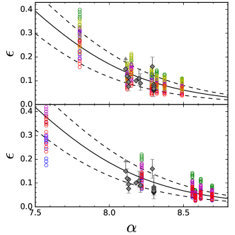
Figure 1: Mean radiative efficiency on the $\epsilon-\alpha$ plane ($\alpha$ is the normalization of the relation between the masses of MBHs and the properties of their host galaxies). Top and bottom panels show the estimates of $\epsilon$ by using the $M_{\bullet}-\sigma$ relation and the $M_{\bullet}-M_{*,\rm sph}$ relation, respectively. In top panel, the blue, green, magenta, red and yellow open circles represent $\epsilon$ estimated by using the VDFs obtained in Sheth et al. [29], Mitchell et al. [30], Choi et al. [31], Bernardi et al. [32] and Sohn et al. [33], respectively; while in the bottom panel, the green, blue, magenta, and red open circles represent $\epsilon$ estimated by using the SMFs obtained in Li and White [35], Bernardi et al. [32], Moustakas et al. [36], and Thanjavur et al. [37], respectively. The solid line in the top panel shows the mean result obtained by setting the slope of the relation $\beta\sim 3.7-5.7$ and using the VDF of Bernardi et al. [32] and XLF of Ranalli et al. [46]; while the solid line in the bottom panel represents the mean results obtained by setting the slope of the relation $\beta\sim 0.75-1.95$, and using the using latest SMF [37] and XLF [46]. The dashed lines in both panels show the $1-\sigma$ uncertainty of the estimates by considering the errors in both the VDF/SMF and XLF. For comparison, the values of mean efficiency obtained in the literature are also shown as grey diamonds.

As discussed above, the uncertainties in the estimates of the mean radiative efficiency ($\epsilon$) of AGNs/QSOs are quite large, which is caused by various reasons, e.g., the uncertainties in the determinations of the relation between the MBH masses and the properties of the MBH host galaxies, in the determinations of the distribution function of galactic properties, and in the estimates of the AGN/QSO luminosity functions. In order to get a more accurate estimate of the mean radiative efficiency, we need to do some statistical analysis. Assuming that all the estimates of $\epsilon$ above are: (1) independent and (2) without systematic effects. These two assumptions are very likely to be valid as the estimates of $\epsilon$ are obtained from a number of independent measurements of the galaxy and AGN/QSO properties, and independent determinations of the relations between the masses of MBHs and the properties of the MBH host galaxies. It is naturally expected that half of the estimates are below the true value and the other half are above the true value. Therefore, we assume the median value obtained from the large number of $\epsilon$ estimates in this paper is close to the true value of $\epsilon$ (and it is the true value if the number of estimates is infinity). This type of median statistics is a powerful tool to deal with a large number of measurements with substantial uncertainties, which has been demonstrated to be extremely useful by Gott et al. [1], e.g., in analyzing the measurements of the Hubble constant and others.

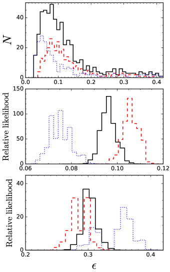
Figure 2: Number distribution of the estimated values for the mean radiative efficiency $\epsilon$ (top panel) and the likelihood distribution of the median of $\epsilon$ (middle panel). The red dashed histogram is for those $\epsilon$ estimated by using the $M_{\bullet}-\sigma$ relation, with median efficiency $0.105^{+0.006}_{-0.008}$. the blue dotted is for those $\epsilon$ estimated by using the $M_{\bullet}-M_{*,{\rm sph}}$ relation, with median value $0.074^{+0.010}_{-0.008}$. The black solid is for all the estimates, and the median efficiency is $0.095^{+0.006}_{-0.007}$. Bottom panel: likelihood distribution of the median efficiency which are derived by applying only the $M_{\bullet}-\sigma/M_{*,{\rm sph}}$ relation of Shankar et al. [26]. Line styles are similar to the top two panels. The median efficiency is $0.272^{+0.032}_{-0.024}$ and $0.349^{+0.033}_{-0.062}$ for the red dashed and blue dotted lines, and is $0.295^{+0.025}_{-0.022}$ for the black solid line. All of the errors above are given at 95% confidence level.

For those estimated $\epsilon$, we rank them as $\epsilon_{i}$ by value such that $\epsilon_{j}>\epsilon_{i}$ if $j>i$. Then the true value of the median lies in between $\epsilon_{i}$ and $\epsilon_{i+1}$ with a probability of

$$P=\frac{2^{-N}N!}{i!(N-i)!}$$ (8)

According to Equation (8), we obtain the true probability distribution of the median of the estimated $\epsilon$.

Figure 2 shows both the number distribution of the estimated value of the mean radiative efficiency $\epsilon$ (top panel) and the probability distributions of the median value of all the estimated $\epsilon$ (middle panel). The red dashed, blue dotted, and black solid histograms in both the two panels show results for $\epsilon$ estimated by using the $M_{\bullet}-\sigma$ relation, the $M_{\bullet}-M_{*,\rm sph}$ relation, and all estimated $\epsilon$, respectively. As seen from Figure 2, the probability distributions of the median $\epsilon$ in the middle panel are much narrower than the number distributions of $\epsilon$ shown in the top panel. According to the probability distributions of the median value of all the estimated $\epsilon$, we find that the median $\epsilon$ is $0.095^{+0.006}_{-0.007}$, where the errors mark the $95\%$ confidence level of the median. If only adopting the values of $\epsilon$ estimated by using the $M_{\bullet}-\sigma$ relation or the $M_{\bullet}-M_{*,\rm sph}$ relation, the median value is then $0.105^{+0.006}_{-0.008}$ or $0.074^{+0.010}_{-0.008}$, respectively. The median obtained by using the $M_{\bullet}-M_{*,\rm sph}$ relation is substantially smaller than that by the $M_{\bullet}-\sigma$ relation. Note that Yu and Tremaine [8] first pointed out that there could be some biases in the determined relation between $M_{\bullet}$ and $M_{*,\rm sph}$, which is lately confirmed by Tundo et al. [48]. This bias may lead to an overestimation of the total MBH mass density by using the $M_{\bullet}-M_{*,\rm sph}$ relation. If only considering the estimates of $\epsilon$ from the $M_{\bullet}-\sigma$ relation, then $\epsilon=0.105^{+0.006}_{-0.008}$, consistent with the canonical value $0.1$ [8].

The above results obtained from the median statistics are valid if there are no systematic biases in all of the measurements of the $M_{\bullet}-\sigma/M_{*,{\rm sph}}$ relations, VDFs/SMFs, and XLFs, which is probably true as those are generally determined by different authors and with (at least partly) different data. One exception is the $M_{\bullet}-\sigma/M_{*,{\rm sph}}$ relation discussed in Shankar et al. [26]. They found that the nearby galaxy sample with MBH mass measurements could be biased from that of the SDSS samples, and the SDSS galaxies have significant higher $\sigma$ than local galaxies with similar stellar mass, as also noted earlier by Yu and Tremaine [8] and Tundo et al. [48]. We therefore repeat the statistical analysis but only for the efficiencies inferred from $M_{\bullet}-\sigma/M_{*,{\rm sph}}$ relation of Shankar et al. [26]. The likelihood distribution is shown in the bottom panel of Figure 2. The median efficiency is $0.272^{+0.032}_{-0.024}$ and $0.349^{+0.033}_{-0.062}$ when the $M_{\bullet}-\sigma$ relation and the $M_{\bullet}-M_{*,\rm sph}$ relation respectively is solely used, and for the total of them, the median value is $0.295^{+0.025}_{-0.022}$.

Note that a fraction of Compton-thick AGNs/QSOs may be still missed from the surveys in the hard X-ray band ($\sim 2-10$ keV) [49]. The fraction of the missed Compton-thick AGNs/QSOs could be $\sim 20\%$ of the total AGN/QSO population [49]. If this is true, then the total energy radiated from AGNs/QSOs over the cosmic time ($E_{\rm tot}$) may be underestimated by $20\%$ in the above analysis, which would lead to an underestimation of the mean radiative efficiency by $\sim 20\%$. The inclusion of those Compton-thick objects may increase the estimated value of the mean radiative efficiency to $\sim 0.12$.

According to the mean radiative efficiency of AGNs/QSOs estimated in this paper ($\epsilon=0.105$ or $\sim 0.12$ by assuming a fraction of $\sim 20\%$ Compton-thick objects), which corresponds to an effective spin of those MBHs $a\sim 0.71$ (or 0.80) if assuming all MBHs in AGNs/QSOs accreting material via the standard thin disk. If only adopting those estimates of $\epsilon$ by using the $M_{\bullet}-\sigma/M_{*,\rm sph}$ relation of Shankar et al. [26], then mean radiative efficiency is $\sim 0.295$, which would correspond to an effective spin of those MBHs $a\gtrsim 0.99$ by further considering the contribution from the missed Compton-thick AGNs/QSOs.

Currently there are about two dozens of MBHs in low redshift AGNs/QSOs that have spin measurements according to the Fe K$\alpha$ line detections [50, 51]. Those MBHs all have intermediate to extremely high spins, i.e., $a\sim 0.4-1$. Those measurements may be still not conclusive, but they seem to be consistent with our estimates about the mean radiative efficiency for the whole population of AGNs/QSOs in this paper. We also note that the radiative efficiency of individual SDSS QSOs has also been estimated by Wu et al. [6], in which the efficiency is estimated by using the bolometric luminosity estimated from multi-wavelength spectra and the accretion rate estimated by fitting the continuum spectra to specific disk accretion model. Wu et al. [6] obtained the mean efficiency of the SDSS QSOs to be about $0.11-0.16$, which is also consistent with the global constraint on the mean radiative efficiency of whole population of AGNs/QSOs obtained in the present paper.

5 Conclusions

The mean radiative efficiency of accretion onto massive black holes (MBHs) in AGNs and QSOs can be estimated by using the Sołtan argument, by matching the mass density of MBHs in the local universe to the accreted mass density by MBHs during AGN/QSO phases. In this paper, we estimate the local MBH mass density through a combination of various determinations of the correlations between the masses of MBHs and the properties of MBH host galaxies, with the distribution functions of those galaxy properties. We also estimate the total energy density radiated by AGNs and QSOs by using various AGN/QSO X-ray luminosity functions in the literature. We obtain several hundred estimates of the mean radiative efficiency of AGNs/QSOs. Under the assumption that all those estimates are independent of each other and free of systematic effects, we apply the median statistics as described by Gott et al.[1] and find the mean radiative efficiency of AGNs/QSOs is $0.095^{+0.006}_{-0.007}$. Considering that roughly $20\%$ Compton-thick objects may be missed from current available X-ray surveys, the mean radiative efficiency may be as high as $\sim 0.11$. However, the efficiency estimated by using the $M_{\bullet}-M_{*,\rm sph}$ relation may be biased. If only those estimates of the efficiency by using the $M_{\bullet}-\sigma$ relation are used, then we find the mean radiative efficiency of AGNs/QSOs is $0.105^{+0.006}_{-0.008}$, which is consistent with the canonical value $\sim 0.1$. Considering the correction due to those Compton-thick objects, the true mean radiative efficiency may be $\sim 0.12$.

This work is partly supported by the National Key Program for Science and Technology Research and Development (Grant No. 2016YFA0400704), the National Natural Science Foundation of China under grant No.11373031 and 11390372, and the Strategic Priority Program of the Chinese Academy of Sciences (Grant No. XDB 23040100).

References

- [1] J. R. Gott, M. S. Vogeley, S. Podariu, and B. Ratra, ApJ, 549, 1 (2001)
- [2] D. Lynden-Bell, Nature, 223, 690 (1969)
- [3] J. M. Bardeen, Nature, 226, 64 (1970)
- [4] W.-H. Sun, and M. A. Malkan, ApJ, 346, 68 (1989)
- [5] S. W.Davis, and A. Laor, ApJ, 728, 98 (2011)
- [6] S. Wu, Y. Lu, F. Zhang, and Lu, Y., MNRAS, 436, 3271 (2013)
- [7] A. Sołtan, MNRAS, 200, 115 (1982)
- [8] Q. Yu, and S. Tremaine, MNRAS, 335, 965 (2002)
- [9] M. Elvis, G. Risaliti, and G. Zamorani, ApJl, 565, L75 (2002)
- [10] A. Marconi, G. Risaliti, R. Gilli, L. K. Hunt, R. Maiolino, M. Salvati, MNRAS, 351, 169 (2004)
- [11] F. Shankar, D. H. Weinberg, and J. Miralda-Escudé, ApJ, 690, 20 (2009)
- [12] Q. Yu, and Y. Lu, ApJ, 602, 603 (2004)
- [13] A. Merloni, G. Rudnick, and T. Di Matteo, MNRAS, 354, L37 (2004)
- [14] X. Cao, ApJ, 659, 950 (2007)
- [15] Q. Yu, and Y. Lu, ApJ, 689, 732 (2008)
- [16] J.-M. Wang, C. Hu, Y.-R. Li, Y.-M. Chen, A. R. King, A. Marconi, L. C. Ho, C.-S. Yan, R. Staubert, S. Zhang, ApJl, 697, L141 (2009)
- [17] E. Treister, C. M. Urry, and S. Virani, ApJ, 696, 110 (2009)
- [18] X. Zhang, Y. Lu, and Q. Yu, ApJ, 761, 5 (2012)
- [19] Y.-R. Li, J.-M. Wang, and L. C. Ho, ApJ, 749, 187 (2012)
- [20] F. Shankar, D. H. Weinberg, and J. Miralda-Escudé, MNRAS, 428, 421 (2013)
- [21] J. Kormendy, and L. C. Ho, ARAA, 51, 511 (2013)
- [22] A. W. Graham, ApJ, 746, 113 (2012)
- [23] R. P. Saglia, M. Opitsch, P. Erwin, J. Thomas, A. Beifiori, M. Fabricius, X. Mazzalay, N. Nowak, S. P. Rusli, and R. Bender, ApJ, 818, 47 (2016)
- [24] S. Tremaine, K. Gebhardt, R. Bender, G. Bower, A. Dressler, S. M. Faber, A. V. Filippenko, V. Alexei, R. Green, C. Grillmair, L. C. Ho, J. Kormendy, T. R. Lauer, J. Magorrian, J. Pinkney, and D. Richstone, ApJ, 574, 740 (2002)
- [25] K. Gültekin, D. O. Richstone, K. Gebhardt, R. R. Lauer, S. Tremaine, M. C. Aller, R. Bender, A. Dressler, S. M. Faber, A. V. Filippenko, R. Green, L. C. Ho, J. Kormendy, J. Magorrian, J. Pinkney, and C. Siopis, ApJ, 698, 198 (2009)
- [26] F. Shankar, M. Bernardi, R. K. Sheth, L. Ferrarese, A. W. Graham, G. Savorgnan, V. Allevato, A. Marconi, R. Läsker, and A. Lapi, MNRAS, 460, 3119 (2016)
- [27] N. Häring, and H.-W. Rix, ApJ, 604, 89 (2004)
- [28] N. J. McConnell, and C.-P. Ma, ApJ, 764, 184 (2013)
- [29] R. K. Sheth, M. Bernardi, P. L. Schechter, S. Burles, D. J. Eisenstein, D. P. Finkbeiner, J. Frieman, R. H. Lupton, D. J. Schlegel, M. Subbarao, K. Shimasaku, N. A. Bahcall, J. Brinkmann, and Z. Ivezić, ApJ, 594, 225 (2003)
- [30] J. L. Mitchell, C. R. Keeton, J. A. Frieman, and R. K. Sheth, ApJ, 622, 81 (2005)
- [31] Y.-Y. Choi, C. Park, and M. S. Vogeley, ApJ, 658, 884 (2007)
- [32] M. Bernardi, F. Shankar, J. B. Hyde, S. Mei, F. Marulli, and R. K. Sheth, MNRAS, 404, 2087 (2010)
- [33] J. Sohn, H. J. Zahid, and M. J. Geller, arXiv: 1704.07843 (2017)
- [34] T. Weinzirl, S. Jogee, S. Khochfar, A. Burket, and J. Kormendy, ApJ, 696, 411 (2009)
- [35] C. Li, and D. M. White, MNRAS, 398, 2177 (2009)
- [36] J. Moustakas, A. L. Coil, J. Aird, M. R. Blanton, R. J. Cool, D. J. Eisenstein, A. J. Mendez, K. C. Wong, G. Zhu, and S. Arnouts, ApJ, 767, 50 (2013)
- [37] K. Thanjavur, L. Simard, A. F. L. Bluck, and T. Mendel, MNRAS, 459, 44 (2016)
- [38] Y. Ueda, M. Akiyama, K. Ohta, and T. Miyaji, ApJ, 598, 886 (2003)
- [39] F. La Franca, F. Fiore, A.Comastri, G. C. Perola, N. Sacchi, M. Brusa, F. Cocchia, C. Feruglio, G. Matt, C. Vignali, N. Carangelo, P. Ciliegi, A. Lamastra, R. Maiolino, M. Mignoli, S. Molendi, and S. Puccetti, ApJ, 635, 864 (2005)
- [40] J. D. Silverman, P. J. Green, W. A. Barkhouse, D.-W. Kim, M. Kim, B. J. Wilkes, R. A. Cameron, G. Hasinger, B. T. Jannuzi, M. G. Smith, P. S. Smith, and H. Tananbaum, ApJ, 679, 118 (2008)
- [41] J. Ebrero, F. J. Carrera, M. J. Page, J. D. Silverman, X. Barcons, M. T. Ceballos, A. Corral, C. R. Della, and M. G. Watson, A & A, 493, 55 (2009)
- [42] B. Yencho, A. J. Barger, L. Trouille, and L. M. Winter, ApJ, 698, 380 (2009)
- [43] J. Aird, K. Nandra, E. S. Laird, A. Georgakakis, M. L. N. Ashby, P. Barmby, A. L. Coil, J.-S. Huang, A. M. Koekemoer, C. C. Steidel, and C. N. A. Willmer, MNRAS, 401, 2531 (2010)
- [44] J. Aird, A. L. Coil, A. Georgakakis, K. Nandra, G. Barro, and P. G. Pérez-González, MNRAS, 451, 1892 (2015).
- [45] S. Fotopoulou, J. Buchner, I. Georgantopoulos, G. Haisinger, M. Salvato, A. Georgakakis, N. Cappelluti, P. Ranalli, L. T. Hsu, M. Brusa, A. Comastri, T. Miyaji, K. Nandra, J. Aird, and S. Paltani, A & A, 587, 142 (2016)
- [46] P. Ranalli, E. Koulouridis, I. Georgantopoulos, S. Fotopoulou, L.-T. Hsu, M. Salvato, A. Comastri, M. Pierre, N. Cappelluti, F. J. Carrera, L. Chiappetti, N. Clerc, R. Gilli, K. Iwasawa, F. Pacaud, S. Paltani, E. Plionis, and C. Vignali, A & A, 590, 80 (2016)
- [47] P. F. Hopkins, G. T. Richards, and L. Hernquist, ApJ, 654, 731 (2007)
- [48] E. Tundo, M. Bernardi, J. B. Hyde, R. K. Sheth, and A. Pizzella, ApJ, 663, 53 (2007)
- [49] A. Malizia, J. B. Stephen, L. Bassani, A. Bird, F. Panessa, and P. Ubertini, MNRAS, 399, 944 (2009)
- [50] L. Brenneman, AcPol, 53, 652 (2013)
- [51] C. S. Reynolds, SSRv, 183, 277 (2014)