Emission Measures and Emission-measure-weighted Temperatures of Shocked ISM and Ejecta in Supernova Remnants

Abstract

A goal of supernova remnant (SNR) evolution models is to relate fundamental parameters of a supernova (SN) explosion and progenitor star to the current state of its SNR. The SNR hot plasma is characterized by its observed X-ray spectrum, which yields electron temperature, emission measure and abundances. Depending on their brightness, the properties of the plasmas heated by the SNR forward shock, reverse shock or both can be measured. The current work utilizes models which are spherically symmetric. One dimensional hydrodynamic simulations are carried out for SNR evolution prior to onset of radiative losses. From these, we derive dimensionless emission measures and emission-measure-weighted temperatures, and we present fitting formulae for these quantities as functions of scaled SNR time. These models allow one to infer SNR explosion energy, circumstellar medium density, age, ejecta mass and ejecta density profile from SNR observations. The new results are incorporated into the SNR modelling code SNRPy. The code is demonstrated with application to three historical SNRs: Kepler, Tycho and SN1006.

1 Introduction

Supernovae (SNe) and supernova remnants (SNRs) have a great impact on the evolution of galaxies and the interstellar medium (ISM) within galaxies (Vink 2012 and references therein). They do this via their energy input into the ISM, and return of elements. The energy content of SNRs is in the forms of: i) the kinetic energy of the unshocked ejecta, shocked ejecta and shocked ISM; and ii) the thermal energy in shocked ejecta and shocked ISM with temperatures $\sim$1 keV. The shocked gas is observed in X-rays. The synchrotron emission from relativistic electrons accelerated by the SNR shockwave is observed in the radio band. There are $\sim$300 observed SNRs in our Galaxy (Green, 2014), but only a small number of the have been well characterized. The vast majority don’t have well-established inferred supernova (SN) type, explosion energy, age or ISM density. Lack of better observational data, including lack of information on the ejecta, is a major obstacle to understanding SNRs. Another important obstacle to characterizing SNRs is the lack of easily-applied models that are still realistic enough to describe SNR evolution.

In order to expedite characterization of a significant number of SNRs, Leahy & Williams (2017) presented a set of SNR evolution models and a software implementation in Python, called SNRPy. That model included forward and reverse shock radius and velocity for all stages of evolution. For modelling observations, emission measures ($EM$) and $EM$-weighted temperatures are required. The above model included $EM$ and $EM$-weighted temperatures for the self-similar early ejecta-dominated (ED) phase (cases (s,n)= (0,7), (0,12) and (2,7)) and self-similar Sedov-Taylor (ST) phase. Even with that limitation, (Leahy, 2017) demonstrated that model fitting of SNRs can give valuable information on the nature of SN explosions. Leahy & Ranasinghe (2018) used the Leahy & Williams (2017) model but with all self-similar ED cases included (s= 0 and 2, n= 6 through 14). In order to model the important ED to ST transition time, that work used a linear interpolation of $EM$ and $EM$-weighted temperatures vs. time between the end of the ED phase and start of the ST phase. The fitting of evolution models to 15 Galactic SNRs showed that Galactic SNRs have the same broad range of explosion energies as LMC SNRs, but occur in significantly denser ISM (Leahy & Ranasinghe, 2018). SNR and SN population properties from models are important inputs to understand the evolution of the Galaxy and its interstellar medium, e.g. Ferrière (2001).

For a typical SNR, with explosion energy $10^{51}$ erg, ejected mass of 1.4 $M_{\odot}$ and ISM density of 1 cm^-3, the ED phase lasts from explosion to 220 yr, the ED to ST transition lasts from 220 yr to 1500 yr, and the ST phase from 1500 yr to onset of radiative cooling at $\sim$15,000 yr. Most X-ray detected Galactic SNRs (e.g. Leahy & Ranasinghe 2018) are either in the ED to ST or the ST phase. Thus quantitative calculations of $EM$s and $EM$-weighted temperatures are needed in order to model X-ray emission from SNRs. A comprehensive and easy-to-use set of $EM$s and $EM$-weighted temperatures have not been presented before, even for the case of spherically symmetric SNR evolution. As late as the ST phase, the shocked ejecta continue to emit X-rays and can be an important diagnostic of the SNR and SN explosion, so calculation of $EM$ and $EM$-weighted temperature is important for both ED to ST and ST phases.

This work focuses on calculating the $EM$s and $EM$-weighted temperatures for the full evolution of an SNR up to the onset of the radiative phase. Section 2 of this paper presents an brief overview of SNR evolution, including the unified SNR evolution introduced by Truelove & McKee (1999). Because of the existence of unified SNR evolution, dimensionless $EM$s and $EM$-weighted temperatures, if available from models for both forward-shocked gas and reverse-shocked gas, serve as a powerful diagnostic tool for the state of an SNR (Leahy & Ranasinghe 2018 and references therein). Section 3 describes the hydrodynamic simulations which include the early ED phase and the late ST phase, and the transition between them (ED to ST). Section 4 describes the results from the hydrodynamic simulations, and analytic fits to dimensionless $EM$s and temperatures. Section 5 gives a summary and where to access the results and the updated SNR modelling code SNRPy. In the appendix we present calculations of $EM$ and $EM$-weighted temperatures for the self-similar ED, ST and cloudy ISM cases.

2 Supernova Remnant Evolution and Structure

A SN explosion creates a SNR starting with the ejection of the SN progenitor envelope at high speed, typically $\sim$10000 km/s, with inner envelope moving more slowly and outer envelope moving more quickly. General descriptions of SNR evolution are given in numerous places (e.g., Cioffi et al. 1988, Truelove & McKee 1999- hereafter TM99, and Leahy & Williams 2017- hereafter LW17). The ejecta collides with the circumstellar medium (CSM) or ISM, causing a foward shock (FS) to propagate outward and a reverse shock (RS) to propagate back into the ejecta.

The general sequence of SNR evolution starts with the ED phase for which the effect of the ejected mass is important. This gradually evolves to the ST phase, for which the swept-up mass by the SN shock far exceeds the ejected mass. For ED, transition and ST phases, radiative energy losses are unimportant. Beyond the ST phase, radiative losses become important (e.g. Cioffi et al. 1988). In the current work, the phases prior to the radiative phases are considered.

The basic interior structure of a SNR, prior to the ST phase, has the following regions from outside to inside: i) the undisturbed CSM; ii) the FS moving into the CSM; a layer of shocked CSM; iii) the contact discontinuity (CD) separating the shocked CSM from the shocked ejecta; iv) the layer of shocked ejecta; v) the RS moving inward relative to the ejecta; and vi) the undisturbed ejecta. The unshocked ejecta has a homologous velocity profile ($v\propto r$ at fixed time).

After the reverse shock reaches the center of the SNR, the entire ejecta is fully shocked. Reflected shocks and sound waves are generated at this time, and die out slowly over time (Cioffi et al., 1988). The reflected shocks and sound waves are clearly seen in the numerical simulations presented below.

In order to calculate SNR evolution and structure, the following simplifying assumptions are made. The SNR is spherically symmetric and radiative losses have not yet set in. This allows us to use the unified SNR evolution model of (Truelove & McKee, 1999), where powerful scaling relations apply. This means that a single set of hydrodynamic calculations can be made, and the results applied to explosions with different explosion energy, different ejecta mass, and different ISM density by using scaling relations. The CSM has: i) constant density; or ii) $1/r^{2}$ stellar wind density profile centered on the SN, i.e., $\rho_{CSM}=\rho_{s}r^{-s}$ with s=0 or s=2. The unshocked ejecta has a constant density core for $r\leq R_{core}$, and a power-law density envelope: $\rho_{ej}\propto r^{-n}$ for $r>R_{core}$.

2.1 Characteristic Scales

Non-radiative supernova remnants undergo a unified evolution (TM99). The characteristic radius and time for $s=0$ are given by $R_{ch}=(M_{ej}/\rho_{0})^{1/3}$ and $t_{ch}=E_{0}^{-1/2}M_{ej}^{5/6}\rho_{0}^{-1/3}$ with $M_{ej}$ the ejected mass and $E_{0}$ the explosion energy. The characteristic velocity is $V_{ch}=R_{ch}/t_{ch}$ and characteristic shock temperature is $T_{ch}=\frac{3}{16}\mu\frac{m_{H}}{k_{B}}V_{ch}^{2}$, with $\mu$ the mean mass per particle. For SNR in a CSM with $s=2$, the characteristic radius and time are given by $R_{ch}=(M_{ej}/\rho_{s})$ and $t_{ch}=E_{0}^{-1/2}M_{ej}^{3/2}v_{w}/\dot{M}$, with $\dot{M}$ and $v_{w}$ the wind mass loss rate and velocity, and $\rho_{s}=\frac{\dot{M}}{4\pi v_{w}}$.

2.2 Emission Measure ($EM$), $EM$-weighted Temperature and Column $EM$

Because the emission from the hot shocked gas in a SNR is dominated by two body processes, it depends on the product of electron and ion densities (e.g. Raymond et al. 1976). $EM$ is defined in terms of electron density $n_{e}$ and hydrogen ion density $n_{H}$ by $EM=\int n_{e}(r)n_{H}(r)dV$. $EM$ can be measured by X-ray observations, so the measured $EM$ is critical to determining the evolution state of a SNR.

$EM$ can be calculated from a model SNR density profile. During self-similar phases of a SNR, the density profile has a constant functional form with normalization and scaling with radius dependent on time. The dimensionless $EM$, $dEM$, was defined by LW17 as $dEM=EM/(n_{e,s}n_{H,s}R_{FS}^{3}$) with $n_{e,s}$ and $n_{H,s}$ are $n_{e}$ and $n_{H}$ immediately inside the forward shock (FS). We extend this to define $dEM_{FS}$ and $dEM_{RS}$ for the gas heated by the FS and for gas heated by the RS, respectively.

$$dEM_{FS} = \frac{1}{n_{e,s}n_{H,s}R_{FS}^{3}}\int_{R_{CD}}^{R_{FS}}n_{e}(r)n_{H}(r)dV$$ (1)

$$dEM_{RS} = \frac{1}{n_{e,s}n_{H,s}R_{FS}^{3}}\int_{R_{RS}}^{R_{CD}}n_{e}(r)n_{H}(r)dV$$ (2)

The observed temperature of a SNR, derived from the X-ray spectrum, depends on the state of the SNR and on the adopted X-ray spectrum model. Commonly used models are one or two component non-equilibrium ionization models. For example, see Maggi et al. 2016 for LMC SNR fits and Leahy & Ranasinghe 2018 for a summary of models for 15 non-historical Galactic SNRs. In some cases, a SNR has an observed multiple-electron temperature plasma which cannot be attributed to the expected two single electron temperature plasmas from forward ISM and reverse shocked ejecta, respectively. ln this case, the plasma is more complicated than the model assumes, and further approximations are required. If there is a dominant electron temperature, the model can be applied assuming the forward or reverse shocked ejecta is dominated by that temperature. If there is not a dominant electron-temperature component, another possible approximation is to use the mean observed electron temperature.

For a single component plasma emission model, the X-ray temperature measures the $EM$-weighted temperature of that component of shocked-heated gas. A strong shock with speed $V_{s}$ heats the ions to the ion shock temperature $kT_{ion}=\frac{3}{16}\mu_{ion}m_{H}V_{s}^{2}$. We use the formula for electron heating by Coulomb collisions described in section 3.1.3 (equation 1) of LW17, which uses the formulation of Cox & Anderson (1982). This gives a steady increase of the ratio of electron temperature to ion temperature from $T_{e}/T_{ion}$=0.03 at age 0 yr to $T_{e}/T_{ion}$=1 at age of $\sim$1000-5000 yr. The latter number depends on CSM density, ejecta mass, and explosion energy. LW17 defined the dimensionless temperature $dT=\frac{1}{T_{FS}}\frac{1}{EM}\int n_{e}(r)n_{H}(r)T(r)dV$, with $T_{FS}$ the forward shock temperature. We extend this to define $dT_{FS}$ and $dT_{RS}$ for the two plasma components heated by the FS and by the RS, respectively.

$$dT_{FS} = \frac{1}{T_{FS}}\frac{1}{EM}\int_{R_{CD}}^{R_{FS}}n_{e}(r)n_{H}(r)T(r)dV$$ (3)

$$dT_{RS} = \frac{1}{T_{FS}}\frac{1}{EM}\int_{R_{RS}}^{R_{CD}}n_{e}(r)n_{H}(r)T(r)dV$$ (4)

The surface brightness of a SNR depends on the line-of-sight integral of the emission coefficient $j(\nu)=n_{e}n_{H}\epsilon(\nu)$, with emissivity $\epsilon(\nu)$. The column emission measure ($CEM$) is often used as a proxy for surface brightness, valid when the emission coefficient is only weakly dependent on the temperature history of the parcel of gas (e.g. see White & Long 1991, herafter WL91). $CEM$ is given by $CEM(B)=\int n_{e}n_{H}dS$, where the integral is along the line of sight through the SNR at impact parameter $B$ from center.

We define the dimensionless $CEM$ using the scaled densities and dimensionless impact parameter, $b=B/R_{FS}$, by

$$cEM(b)=\int\frac{n_{e}(x(s))}{n_{e,s}}\frac{n_{H}(x(s))}{n_{H,s}}ds$$ (5)

with $s=S/R_{FS}$ and $x(s)=\sqrt{b^{2}+s^{2}}$. More generally, we define the dimensionless $cEM(b)$ separately for gas heated by the forward shock and gas heated by the reverse shock, dimensionless $cEM_{FS}(b)$ and $cEM_{RS}(b)$. For $cEM_{FS}(b)$, $x(s)$ is limited to values between $R_{CD}/R_{FS}$ and 1, while for $cEM_{RS}(b)$, $x(s)$ is limited to values between $R_{RS}/R_{FS}$ and $R_{CD}/R_{FS}$.

3 Hydrodynamic Calculations of SNR Structure

To calculate the interior structure of a SNR, we use the hydrodynamic equations. The evolution follows a unified evolution as shown by TM99, before radiative losses become important. Unified evolution means that solutions have the same dependence on $t/t_{ch}$ if radius is scaled by $R_{ch}$, velocity is scaled by $V_{ch}$ and temperature is scaled by $T_{ch}$. Because there is no smooth transition for s=2 from ED to post-ED (e.g. TM99), we calculate the post-ED phases only for the s=0 case. That evolution is the subject of this section.

The evolution of $R_{FS}$ and $R_{RS}$ has been calculated using an analytic approximation for ED, ED to ST and ST phases by TM99. The reverse shock slows its outward motion relative to the ISM at about the time that it reaches the ejecta core, at time $t_{core}$ (TM99). Then it propagates inward, reaching the center of the SNR at time $t_{rev}$ (TM99). The evolution is continuous, but it is useful to label the phases as ‘ED’ for $0<t<t_{core}$, ‘ED to ST’ for $t_{core}<t<t_{rev}$, and ‘ST’ for $t_{rev}<t<t_{PDS}$, where $t_{PDS}$ is the time where radiative losses affect the evolution (Cioffi et al. 1988, TM99 and LW17). However, the ‘ST’ phase can be quite different that the ‘pure ST’ evolution, as pointed out by LW17.

Here we calculate the evolution and interior structure for s=0 and n=6 to 14 using the hydrodynamics code PLUTO (Mignone et al. 2007, Mignone et al. 2012). A core-envelope structure for the ejecta is assumed. For the simulations the fundamental code units were set to $\rho_{u}=10^{-18}$ gm/cm^-3 (density), $r_{u}=10^{16}$ cm (distance) and $v_{u}=10^{7}$ cm/s (velocity). The resulting code units for time, pressure, mass and energy are $t_{u}=10^{9}$ s, $P_{u}=10^{-4}$ dyne cm^-2 , $M_{u}=10^{30}$ gm and $E_{u}=10^{44}$ erg.

We tested different values for the ISM density, ejecta mass and explosion energy to verify that SNR evolution in scaled variables (density scaled by $\rho_{ISM}$, time scaled by $t_{ch}$, radius by $R_{ch}$, velocity by $V_{ch}$ and pressure by $P_{ch}=\rho_{ISM}V_{ch}^{2}$) was independent of those initial quantites. Then we set the ISM density $=10^{-22}$gm/cm³, ejected mass $=1~{}M_{\odot}$, and explosion energy $=10^{51}$ erg for the remaining calculations. This yields characteristic scales of $t_{ch}=3.839\times 10^{9}$ s $=121.7$ yr, $R_{ch}=2.714\times 10^{18}$ cm $=0.8797$ pc, $V_{ch}=7.071\times 10^{3}$ km/s and $P_{ch}=5.000\times 10^{-5}$ dyne cm^-2.

The SNR initial conditions were initially taken to be an unshocked ejecta with core and envelope components, plus shocked and unshocked ISM. The resulting time-dependent solutions showed large transient fluctuations in the hydrodynamic variables. Use of more accurate initial conditions should result in smaller transient fluctuations. Thus a more accurate second case of initial conditions was constructed from the self-similar Chevalier-Parker (CP, Chevalier 1982, Parker 1963) solutions, consisting of unshocked and shocked ejecta, and shocked and unshocked ISM.

For the first case initial conditions, a small outer ejecta radius $R_{ej}=5\times 10^{12}$ cm was chosen. The core radius was taken as $10^{-1.5}$ of $R_{ej}$. The core density was set so that the integrated mass from $r=0$ to $r=R_{ej}$ was 1 $M_{\odot}$. The velocity increases linearly with radius for the unshocked ejecta, so the velocity profile is specified by the velocity $v_{ej}$ at $r=R_{ej}$. $v_{ej}$ was determined by requiring the total ejecta kinetic energy to be the explosion energy. For example, $v_{ej}=2.888\times 10^{5}$ km/s and $v_{core}=9.132\times 10^{3}$ km/s is found for n=7. The ejecta pressure was set to a low value ($10^{-8}$ dyne cm^-2).

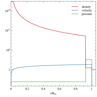
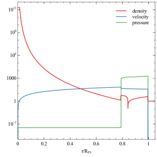
Figure 1: Simulation of an SNR with s=0, n=7: Left panel: initial conditions of unshocked ejecta and shocked ISM at t=$4.5\times 10^{-8}$, $R_{FS}$=$2.0\times 10^{-6}$. Right panel: initial conditions using CP self-similar solution of shocked ejecta and shocked ISM at t=$4.1\times 10^{-5}$, $R_{FS}$=$3.3\times 10^{-3}$. Density, velocity, pressure, time t and forward shock radius $R_{FS}$ are in characteristic units, the x-axis is in units of $r/R_{FS}$.

A layer of shocked ISM with density 4 $\rho_{ISM}$ was added outside the ejecta from $R_{ej}$ to $R_{FS,0}$. The outer initial forward shock radius is $R_{FS,0}=(13/12)R_{ej}$, determined from the requirement that the mass of shocked ISM equals the total ISM mass swept up between $r=0$ and $R_{FS,0}$. The velocity of the layer is $v_{ej}$, because the high density at early times of the ejecta makes it act like a rigid piston. This yields a shock velocity at $R_{FS,0}$ of $v_{FS,0}=(4/3)v_{ej}$ and an interior pressure of the ejecta layer of $(3/4)\rho_{ISM}v_{FS,0}^{2}$. Including the time for the outer edge of the ejecta to expand to $R_{ej}$ from $r=0$, the initial solution has $t/t_{ch}=4.5\times 10^{-8}$ and $R_{FS}/R_{ch}=1.99\times 10^{-6}$ for n=7. The initial conditions for the n=7 simulation are shown in the left panel of Fig. 1.

The second case for the initial conditions utilizes the CP self-similar solutions. The initial density profile is determined by matching both the unshocked ISM and the unshocked ejecta to the CP solution. The outer boundary of the CP solution at $R_{FS,0}$ is set to $4\rho_{ISM}$, and the outer boundary of the unshocked ejecta at $R_{RS,0}$ is set to $(1/4)\rho_{CP}(R_{RS,0})$ from the CP solution.

The ejecta mass includes the core, $r<R_{core}$, the unshocked powerlaw envelope, $R_{core}$ to $R_{RS}$, and the shocked ejecta, $R_{RS}$ to $R_{CD}$. The shocked ejecta contains a pileup of the shocked envelope mass.We define $w_{core}=R_{core}/R_{RS}$, which is different than TM99 who don’t have a layer of shocked ejecta in their initial density profile. We set $w_{core}=10^{-1.5}$. For small $w_{core}$, the contribution from the shocked ejecta is small. Thus we use the analytic value of mass from the unshocked ejecta, $M_{ej}\simeq M_{core}+M_{env}=M_{core}\frac{n-3w_{core}^{n-3}}{n-3}$ to obtain the initial estimate of $M_{core}$ from $M_{ej}$. We integrate to obtain an accurate value of all three contributions to the ejecta mass. Then we set the total to the desired ejecta mass, $1M_{\odot}$, to determine a more accurate value of $M_{core}$ . $\rho_{core}$ is found from $M_{core}=(4/3)\pi R_{core}^{3}\rho_{core}$ for given $R_{core}$. $R_{core,0}$ is chosen large enough to be resolved with enough grid cells in the hydrocode. It is small enough to give $R_{FS,0}<<R_{ch}$, to include enough of the early ED phase prior to the post-ED evolution. E.g., for n=7 we chose $R_{core,0}=4.0\times 10^{14}$ cm, yielding $R_{FS,0}=1.60\times 10^{16}$ cm $=3.31\times 10^{-3}R_{ch}$.

The initial estimate of $v_{core}$ is obtained from the energy of core and unshocked envelope. This is given by $E_{ej}\simeq E_{core}+E_{env}=E_{core}\frac{n-5w_{core}^{n-5}}{n-5}$ and $E_{core}=(2/5)\pi R_{core}^{3}\rho_{core}v_{core}^{2}$. The error in $v_{core}$ is small for small $w_{core}$. A more accurate $v_{core}$ is obtained by integrating the energy in the core, unshocked envelope and the shocked envelope and setting to the explosion energy, $10^{51}$ erg. The velocity at the outer edge of the unshocked envelope is $v_{env}=v_{core}\times R_{RS,0}/R_{core,0}$. The time since explosion for the initial solution is given by $t_{0}=R_{core,0}/v_{core}$. For n=7, $v_{core}=9.13\times 10^{3}$ km/s and $t_{0}/t_{ch}=4.14\times 10^{-5}$.

To match velocities with the CP solution, we apply shock jump conditions at both forward and reverse shocks. The postshock pressure at $R_{FS}$ is $P_{FS}=(3/4)\rho_{ISM}V_{FS}^{2}$. The pressure ratio $x_{RF}=P_{RS}/P_{FS}$ is an n-dependent constant given by the CP solution. The reverse shock velocity, relative to the envelope gas, is $P_{RS}=(3/4)\rho_{env}V_{RS}^{2}$ with the reverse shock velocity in the envelope frame $V_{RS}=v_{env}-V_{RS,obs}$ with $V_{RS,obs}$ the reverse shock velocity in the observer frame. The gas velocity relative to the post-shock gas $v_{sh,rel}$ is 1/4 of the pre-shock gas $v_{un,rel}$: $v_{sh,rel}=(1/4)v_{un,rel}$. After a bit of algebra we find:

$$V_{FS}=\frac{4~{}v_{env}}{3(\sqrt{y_{RF}~{}\rho_{ISM}/\rho_{env}}+y_{RF})}$$ (6)

where the ratio of post-shock gas velocities from the CP solution is given by $y_{RF}=v_{sh,RS}/v_{sh,FS}$.

The above procedure fully determines the initial conditions which satisfy the shock jump conditions at both shocks and have the correct total energy and ejecta mass. The initial CP solution for n=7 is shown in the right panel of Fig. 1. This has $v_{env,0}=2.89\times 10^{5}$ km/s and $V_{FS,0}=2.09\times 10^{5}$ km/s.

The initial conditions for case 1 were computed analytically using a modified init.c program in PLUTO. The initial conditions for case 2 consist of a binary file which includes the CP numerical solutions matched to the unshocked ejecta and and the ISM. For both cases, we added a passive scalar tracer field to track the contact discontinuity and the ejecta core-envelope boundary.

The SNR evolution includes a large range in time and spatial scales. The typical initial time is $\sim 10^{-8}t_{ch}$ (case 1) to $10^{-4}t_{ch}$ (case 2) and initial radius is $\sim 10^{-6}R_{ch}$ (case 1) to $10^{-3}R_{ch}$ (case 2). For case 1, we started the simulation at very early time and small radius in order to allow the approximate initial conditions to relax to a more accurate solution. The late stage time is $\sim 10^{4}t_{ch}$ and late stage radius is $\sim 10^{2}$ $R_{ch}$, for both cases. Thus it is not possible to compute the SNR structure in a single run of PLUTO. Instead we ran the code successively in stages, with the output of each stage used as input for the next stage. The computational grid was chosen so that the SNR initial outer shock radius was $\simeq$1/5 of the grid size which allowed room for the SNR to expand to the edge of the grid before initiating a new stage. The spatial grid size was chosen 5000 points, so the SNR was resolved by a minimum of 1000 points at any time. Typically, 7 to 10 stages were computed for each evolution, allowing a $\simeq 10^{5}~{}-~{}10^{8}$ factor in radial expansion. The time steps were adjusted by PLUTO to satisfy the Courant condition, yielding $\sim 80,000$ timesteps per stage. The times for saving structure files (or snapshots) of the evolution were chosen manually, resulting in $\sim 250$ snapshots per evolution.

4 Results and Discussion

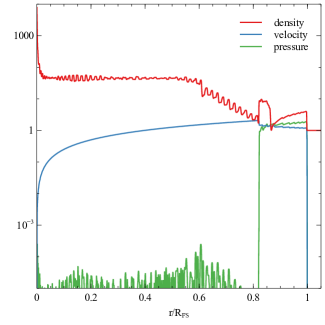
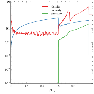
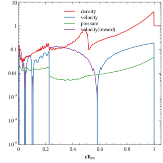
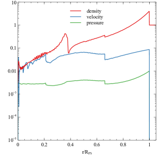
Figure 2: Snapshots of the interior structure for s=0, n=8 from hydrodynamic simulations at 4 characteristic times: $t/t_{ch}\simeq 0.10$ with $R_{FS}/R_{ch}\simeq 0.27$ (top left), $t/t_{ch}\simeq 1.1$ with $R_{FS}/R_{ch}\simeq 1.1$ (top right), $t/t_{ch}\simeq 3.1$ with $R_{FS}/R_{ch}\simeq 1.8$ (bottom left) and $t/t_{ch}\simeq 10$ with $R_{FS}/R_{ch}\simeq 2.9$ (bottom right). The density, velocity and pressure are scaled to their characteristic values, and are plotted vs. radius in units of the forward shock radius ($r/R_{FS}$). Inward gas velocities are plotted in purple in the bottom left panel.

The evolution of the interior density, velocity and pressure is captured in the snapshots from PLUTO vs. time. Because of the homologous velocity profile of unshocked ejecta ($v\propto r$), the density interior to the RS drops as $1/t^{3}$ and the core-envelope boundary expands linearly with time. These properties are reproduced by the hydro simulations, with both cases of initial conditions. Numerical errors are visible in the results, e.g. the top two panels of Fig. 2. The relative errors are largest in unshocked ejecta pressure because the initial pressure is small in that region. Errors in density are small except at the origin, and velocity errors are small everywhere. Case 1 hydro solutions have larger errors than case 2.

Evidence that the solutions are reliable comes from comparison of the solutions with different initial conditions. Despite large differences in the initial conditions, both case 1 and case 2 evolve to the same structure after time of $t\simeq 0.01t_{ch}$. The $t<0.01t_{ch}$ differences between the case 1 hydro solution and the case 2 hydro solution can be attributed to the inaccuracy of the case 1 initial conditions. Because the simulations for case 1 and case 2 agree after $t\simeq 0.01t_{ch}$, and the fluctuations for case 2 are smaller than for case 1, hereafter we use the results from case 2.

The self similar evolution of the interior structure from early times ($t<<t_{ch}$) was verified. Deviations from self-similar evolution as time increases are expected. These deviations are apparent starting at $t\simeq 0.3t_{ch}$ when reverse shock propagates inward to reach the the core boundary. After this time $R_{RS}/R_{FS}$ decreases. This can be seen in the animations of the structure files provided with this paper. At $t/t_{ch}=1$, $R_{RS}$ is well inside the core (top right panel of Fig. 2), and a sawtooth shape density forms just inside the CD. This sawtooth density at the CD persists for the remainder of the SNR evolution.

After $t/t_{ch}=1$, the reverse shock accelerates inward, reaching the SNR center at $t/t_{ch}\simeq 2.5$, in agreement (within $\sim 10\%$) with the results of TM99. After the RS hits the center, a reflected shock slowly propagates outward. In the bottom left panel of Fig. 2, for $t/t_{ch}\simeq 3$, the reflected shock is propagating outward and is visible as the pressure, velocity and density jumps at $r/R_{FS}=0.2$. The reflected shock reaches $r/R_{FS}=0.7$ at $t/t_{ch}\simeq 10$ (bottom right panel of Fig. 2), and finally reaches the forward shock at $t/t_{ch}\simeq 80$.

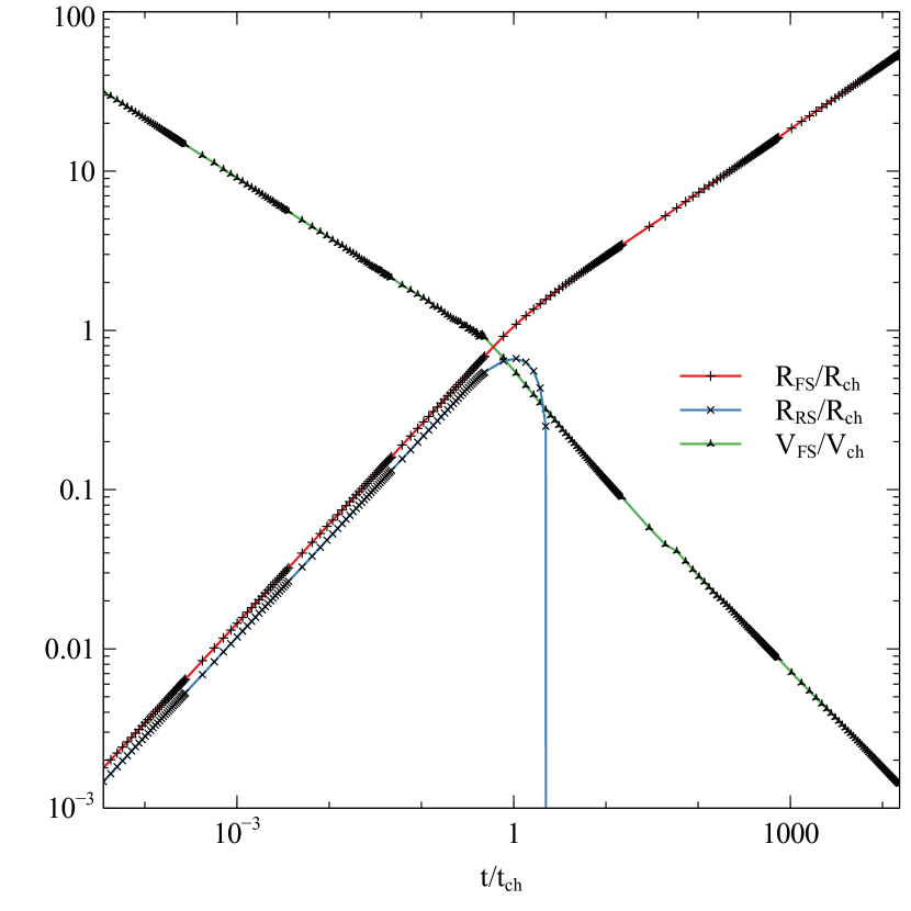
Figure 3: Forward shock radius $R_{FS}$ and velocity $V_{FS}$, and reverse shock radius $R_{RS}$ extracted from the hydrodynamic simulations for s=0, n=8. Quantities are plotted as in units of characteristic radius or velocity as a function of characteristic time, $t/t_{ch}$.

The evolution for s=0, n=8 of $R_{FS}$, $V_{FS}$ and $R_{RS}$ is shown in Fig. 3. The deviation from self-similar behaviour is seen at $t/t_{ch}\simeq 0.3$. The reverse shock moves inward after $t/t_{ch}\simeq 1$ and hits the SNR center at $t/t_{ch}\simeq 2.5$. A perturbation in $V_{FS}$ is seen when the reflected shock hits the FS at $t/t_{ch}\simeq 80$.

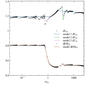
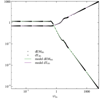
Figure 4: Extracted quantities from the hydrodynamic simulations for s=0, n=8 as a function of characteristic time, $t/t_{ch}$. Left: dimensionless temperature $dT_{FS}$ and dimensionless emission measure $dEM_{FS}$ of forward-shocked gas. Right: dimensionless temperature $dT_{RS}$ and dimensionless emission measure $dEM_{RS}$ of reverse-shocked gas. The functions fit to $dT_{FS}$, $dEM_{FS}$, $dT_{RS}$ and $dEM_{RS}$ vs. $t/t_{ch}$ are shown by the lines labelled model.

Fig. 4 (left) shows $dEM$ and $dT$ for FS shocked gas for n=8. $dEM_{FS}$ and $dT_{FS}$ vary weakly with time, with maximum range of $\simeq 0.8-0.5$ for $dEM_{FS}$, and $\simeq 1.1-1.3$ for $dT_{FS}$. By comparing different runs with different n, case 1 and case 2 initial conditions, and with other varied parameters, and by examining the physical variables in the animations, we determined that the decrease near $t/t_{ch}\simeq 0.6$ and the changes at $t/t_{ch}\simeq 60$ are real.

In the animations of hydrodynamic variables, one can see the reverse shock encounter the ejecta core at $t/t_{ch}\simeq 0.25$. Then between $t/t_{ch}\simeq 0.4$ and $\simeq 0.8$, the density profile of the shocked ejecta changes from a nearly square-wave shape to a saw-tooth shape (compare the first two panels in Fig. 2). Over the same time interval the density profile of shocked ISM changes from nearly flat just inside the forward shock to steeply decreasing inward from the forward shock. While this is happening, the pressure profile of both reverse and forward shocked gas changes from being nearly flat to steeply increasing with radius (compare the first two panels in Fig. 2). The change in temperature and density profiles combined between $t/t_{ch}\simeq 0.4$ and $\simeq 0.8$ yields an EM-weighted temperature drop compared to the temperature at the forward shock.

At $t/t_{ch}\simeq 2.5$ the reverse shock converges to the center and bounces back outward. This reflected shock passes through the CD at $t/t_{ch}\simeq 5$ and reaches the forward shock at $t/t_{ch}\simeq 60$. It then reflects back inward slowly, not reaching the CD even at the end of the simulations at $t/t_{ch}\simeq 10^{4}$. Meanwhile a second reflected shock, produced from the ejecta density peak at $t/t_{ch}\simeq 5$, propagates inward reaching the center at $t/t_{ch}\simeq 7$. This second reflected shock propagates out to reach the CD at $t/t_{ch}\simeq 13$. The interior temperature and density profiles of forward-shocked ISM (outside the CD) gradually steepen with time between $t/t_{ch}\simeq 5$ and $t/t_{ch}\simeq 60$, but don’t change significantly after that. A drop near $t/t_{ch}\simeq 60$ in $dT_{FS}$ is seen in the first panel of Fig. 4. This is seen in our simulations for all values of n. This is likely caused by the change in density and pressure profiles caused by the reflected shock encountering the forward shock. Because the EM-weighted temperature is dominated by the densest gas in a small region around the forward shock, it can be significantly affected at the time the reflected shock encounters the forward shock.

Fig. 4 (right) shows $dEM$ and $dT$ for RS shocked gas for n=8. For RS shocked gas, $dEM_{RS}$ and $dT_{RS}$ change rapidly with time after the early self-similar phase. $dEM_{RS}$ and $dT_{RS}$ both show a significant increase around $t/t_{ch}\simeq 5$, which is real and caused by the first reflected shock encountering the density peak in the shocked ejecta.

4.1 Fits to $dEM$ and $dT$ from the hydrodynamic SNR solutions

In order to facilitate usage of $dEM$ and $dT$ for modelling SNRs, we provide fitting functions to $dEM$ and $dT$ for both FS and RS gas. $dEM_{FS}$, $dT_{FS}$, $dEM_{RS}$ and $dT_{RS}$ were extracted from the hydro simulations for n= 6 to 14, as functions of scaled time $t_{s}=t/t_{ch}$. We found that piecewise powerlaw functions provide good approximations (i.e. fractional errors less than 5%) to these quantities. The minimum number of segments was chosen to give a good fit to the data using least squares minimization.

Fig. 4 shows the extracted $dEM$ and $dT$ for n=8 and the n=8 fitting functions. Because $dT_{FS}$ has the most complex behaviour, we show three different fits: one with 6 segments; a second with 5 segments; and a third with 3 segments. The 6 segment function gives the best fit to the simulation $dT_{FS}$ values, and the 3 segment function fits a smoothed version of $dT_{FS}$. Because real SNRs are not completely spherically symmetric, the RS from different directions is expected to encouter the ejecta core and to hit the SNR center at slightly different times. Thus a real SNR is expected to have a smoother peak in $dT_{FS}$ at both $t/t_{ch}\simeq 0.6$ and $t/t_{ch}\simeq 60$, compared to our hydro simulations.

We thus chose to use the 3 segment fit to the smoothed $dT_{FS}$ here, for all n values, given by:

$$dT_{FS}(t_{s}) = dT_{FS,0}\qquad\qquad\qquad\qquad\qquad~{}~{}~{}~{}~{}if~{}~{}t_{s}<t_{1}$$

$$dT_{FS,0}(t_{s}/t_{1})^{p_{1}}\qquad\qquad\qquad\qquad~{}~{}if~{}~{}t_{1}<t_{s}<t_{2}$$

$$dT_{FS,0}(t_{2}/t_{1})^{p_{1}}(t_{s}/t_{2})^{p_{2}}\qquad\qquad~{}~{}~{}if~{}~{}t_{2}<t_{s}$$

For $dEM_{FS}$, a model with 5 segments fits the simulation results:

$$dEM_{FS}(t_{s}) = dEM_{FS,0}~{}~{}~{}~{}~{}~{}~{}~{}~{}~{}~{}~{}~{}~{}~{}~{}~{}~{}~{}~{}~{}~{}~{}~{}~{}~{}~{}~{}~{}~{}~{}~{}~{}~{}~{}~{}~{}~{}~{}~{}~{}~{}~{}~{}~{}if~{}~{}t_{s}<t_{1}$$

$$dEM_{FS,0}(t_{s}/t_{1})^{p_{1}}~{}~{}~{}~{}~{}~{}~{}~{}~{}~{}~{}~{}~{}~{}~{}~{}~{}~{}~{}~{}~{}~{}~{}~{}~{}~{}~{}~{}~{}~{}~{}~{}~{}~{}~{}~{}if~{}~{}t_{1}<t_{s}<t_{2}$$

$$dEM_{FS,0}(t_{2}/t_{1})^{p_{1}}(t_{s}/t_{2})^{p_{2}}~{}~{}~{}~{}~{}~{}~{}~{}~{}~{}~{}~{}~{}~{}~{}~{}~{}~{}~{}~{}~{}~{}~{}~{}~{}if~{}~{}t_{2}<t_{s}<t_{3}$$

$$dEM_{FS,0}(t_{2}/t_{1})^{p_{1}}(t_{3}/t_{2})^{p_{2}}(t_{s}/t_{3})^{p_{3}}~{}~{}~{}~{}~{}~{}~{}~{}~{}~{}~{}~{}~{}~{}if~{}~{}t_{3}<t_{s}<t_{4}$$

$$dEM_{FS,0}(t_{2}/t_{1})^{p_{1}}(t_{3}/t_{2})^{p_{2}}(t_{4}/t_{3})^{p_{3}}(t_{s}/t_{4})^{p_{4}}~{}~{}~{}if~{}~{}t_{4}<t_{s}$$

The right panel of Fig. 4 shows $dEM$ and $dT$ for RS shocked gas. After $t/t_{ch}\sim 0.3$, $dEM_{RS}$ decreases and $dT_{RS}$ increases. The main cause of the decrease of $dEM_{RS}$ is the increase of volume of FS gas (via $R_{FS}$) relative to volume of RS gas (see equation 2). The main cause of the increase of $dT_{RS}$ is the decrease of $T_{FS}$ relative to slower decrease of $T$ of RS gas (see equation 4).

For $dT_{RS}$ and for $dEM_{RS}$, 4 segments fit the simulation results:

$$dT_{RS}(t_{s}) = dT_{RS,0}~{}~{}~{}~{}~{}~{}~{}~{}~{}~{}~{}~{}~{}~{}~{}~{}~{}~{}~{}~{}~{}~{}~{}~{}~{}~{}~{}~{}~{}~{}~{}~{}~{}~{}~{}~{}~{}~{}~{}~{}~{}if~{}~{}t_{s}<t_{1}$$

$$dT_{RS,0}(t_{s}/t_{1})^{p_{1}}~{}~{}~{}~{}~{}~{}~{}~{}~{}~{}~{}~{}~{}~{}~{}~{}~{}~{}~{}~{}~{}~{}~{}~{}~{}~{}~{}~{}~{}~{}~{}if~{}~{}t_{1}<t_{s}<t_{2}$$

$$dT_{RS,0}(t_{2}/t_{1})^{p_{1}}(t_{s}/t_{2})^{p_{2}}~{}~{}~{}~{}~{}~{}~{}~{}~{}~{}~{}~{}~{}~{}~{}~{}~{}~{}~{}~{}~{}if~{}~{}t_{2}<t_{s}<t_{3}$$

$$dT_{RS,0}(t_{2}/t_{1})^{p_{1}}(t_{3}/t_{2})^{p_{2}}(t_{s}/t_{3})^{p_{3}}~{}~{}~{}~{}~{}~{}~{}~{}~{}~{}~{}if~{}~{}t_{3}<t_{s}$$

.

$$dEM_{RS}(t_{s}) = dEM_{RS,0}~{}~{}~{}~{}~{}~{}~{}~{}~{}~{}~{}~{}~{}~{}~{}~{}~{}~{}~{}~{}~{}~{}~{}~{}~{}~{}~{}~{}~{}~{}~{}~{}~{}~{}~{}~{}~{}~{}~{}~{}if~{}~{}t_{s}<t_{1}$$

$$dEM_{RS,0}(t_{s}/t_{1})^{p_{1}}~{}~{}~{}~{}~{}~{}~{}~{}~{}~{}~{}~{}~{}~{}~{}~{}~{}~{}~{}~{}~{}~{}~{}~{}~{}~{}~{}~{}~{}~{}~{}if~{}~{}t_{1}<t_{s}<t_{2}$$

$$dEM_{RS,0}(t_{2}/t_{1})^{p_{1}}(t_{s}/t_{2})^{p_{2}}~{}~{}~{}~{}~{}~{}~{}~{}~{}~{}~{}~{}~{}~{}~{}~{}~{}~{}~{}~{}~{}if~{}~{}t_{2}<t_{s}<t_{3}$$

$$dEM_{RS,0}(t_{2}/t_{1})^{p_{1}}(t_{3}/t_{2})^{p_{2}}(t_{s}/t_{3})^{p_{3}}~{}~{}~{}~{}~{}~{}~{}~{}~{}~{}if~{}~{}t_{3}<t_{s}$$

The best fit coefficients for $dT_{FS}(t_{s})$, $dEM_{FS}(t_{s})$, $dT_{RS}(t_{s})$ and $dEM_{RS}(t_{s})$ are given in Table 1 for the different values of n. $dT_{FS,0}$, $dEM_{RS,0}$, $dT_{FS,0}$ and $dEM_{RS,0}$ were fixed at the values for the initial CP self-similar phase for s=0 and the different n values.

In general terms, the dividing times between the segments of nearly powerlaw behaviour correspond to changes in the interior physical structure, either pressure or density, of the SNR. The first segment covers the self-similar early ED phase, and ends near, or soon after, the time when the inward moving (in the frame of the ejecta) reverse shock encounters the power-law core of the ejecta. For the shocked-ISM quantity $dEM_{FS}$, the end of the second segment is near the time that the density and pressure profiles of the shocked-ISM steepen (seen in the animations). The end of the third segment is near the time that the reflected shock propagates to the inner boundary of the shocked-ISM and starts to flatten the density and pressure profiles. The end of the fourth segment is when the reflected shock reaches the forward shock at $t/t_{ch}\simeq 50$. The fifth segment lasts from that time onward.

The shocked-ISM quantity, $dT_{FS}$, the simplified 3 segment fits shown here have two transition times. The physical transitions times are as noted in the above paragraph. The best-fit transition times are phenomenological. The first is intermediate between the time of reverse shock encountering the ejecta core and when it reaches the center. The second is intermediate between the time of reflected shock encountering the inner edge of shocked ISM and the time when it encouters the forward shock.

For the shocked-ejecta quantities, $dEM_{RS}$ and $dT_{RS}$, the end of the second segment is near the time that the reverse shock reaches the SNR center. The end of the third segment is near the time that the reflected shock propagates outward to reach the peak in density of the shocked ejecta. The fourth segment lasts from that time, $t/t_{ch}\simeq 5$, onward.

With the calculated time-dependent $dEM$ and $dT$, we can compare how the properties of the shocked ISM and shocked ejecta change with time. The FS EM and EM-weighted T, in dimensionless form, remain remarkably constant over the whole SNR evolution: From Fig. 4 (left), we see that $dT_{FS}$ only rises a small amount ($\sim 10$%) between $t/t_{ch}$ = 1 and 10, whereas significant changes in $dT_{RS}$ and $dEM_{RS}$ occur. The very slow decrease of $dT_{FS}$ after $t/t_{ch}\sim 100$ occurs in all the simulations, providing evidence it is a real effect. This decrease is probably caused by the effect of the reflected shock on expanding the forward shock more than it does in the self-similar solution. $dEM_{FS}$ exhibits small changes, with a sharp decrease of $\sim 40$% between $t/t_{ch}$ = 0.4 and 2, during the time the reverse shock propagate through the ejecta core.

For shocked ejecta, $dT_{RS}$ rises steadily with time after the self-similar phase ends, near $t/t_{ch}$ = 0.3, and has a bump around $t/t_{ch}\simeq$6, when the reflected shock passes through the dense shell of ejecta near the CD. We find that the shocked ejecta is hotter than the shocked ISM ($dT_{RS}>dT_{FS}$) for $t/t_{ch}\gtrsim$ 2 for n=6. This transition of $T_{RS}>T_{FS}$ (noting that the scaling is the same for both values to obtain dimensionless values) gradually increases from $t/t_{ch}\gtrsim$ 2 for n=6 to $t/t_{ch}\gtrsim$ 4 for n=14.

$dEM_{RS}$ (right panel of Fig. 4) decreases steadily with time after the self-similar phase ends, near $t/t_{ch}$ = 0.3, and has a bump around $t/t_{ch}\simeq$ 6, caused by the reflected shock. The $EM$ of shocked ejecta is smaller than that of shocked ISM ($dEM_{RS}<dEM_{FS}$) at all times for n=6 and 7. For n=8 to 14, $dEM_{RS}>dEM_{FS}$ at early times and $dEM_{RS}<<dEM_{FS}$ at late times. The transition time for the $EM$ of shocked ISM to exceed that of shocked ejecta increases from $t/t_{ch}$ = 0.4 for n=8 to $t/t_{ch}$ = 0.6 for n=14.

There are other small changes in $dT_{FS}$, $dEM_{FS}$ , $dT_{RS}$ and $dEM_{RS}$. Comparison with the hydro simulations snapshots shows that these are caused by the RS shock encountering then propagating rapidly through the ejecta core, reflecting from convergence at the SNR center, and then propagating outward through the shocked ejecta, the CD and the shocked ISM to the FS.

4.2 Application of the Model to SNR Observations

In order to demonstrate the current model, we apply it to three historical Galactic SNRs with published electron temperatures and emission measures: Kepler, Tycho and SN1006. The model is applied to the FS emission of each SNR to test if the model can reproduce the observed FS radius, FS emission measure, FS temperature and the known SNR age. Table Emission Measures and Emission-measure-weighted Temperatures of Shocked ISM and Ejecta in Supernova Remnants gives the observed age, type, radius, FS emission measure and FS temperature for these SNRs. All three SNRs are Type Ia, so we use an estimated ejected mass of 1.2$\textrm{M}_{\sun}$, and also test models with 1.0$\textrm{M}_{\sun}$ and 1.4$\textrm{M}_{\sun}$. In the following sections, we discuss the model results and implications.

Table 3 gives the observed shocked ejecta (RS) emission measures and temperatures. Kepler and Tycho each have three measured ejecta components and SN1006 has two measured ejecta components. The observations indicate that layering of the ejecta is important in all three SNRs. The current model is simplified and assumes the ejecta is uniformly mixed. We do not explore the complication of ejecta layering in the current model but leave that to future work.

4.2.1 G$4.5+6.8$ (Kepler)

The remnant of the Kepler’s SN of 1604 is a well studied SNR. Kinugasa & Tsunemi (1999) analyse the relative abundances of the ejecta to classify Kepler’s SN as a Type Ia SN. The distance to the $3^{\prime}$ diameter SNR has been a difficult obtain. The estimates range from a lower limit of 3.0 kpc (Sankrit et al., 2005) to an upper limit of 6.4 kpc (Reynoso, & Goss, 1999). For this study we use the distance of $5.1^{+0.8}_{-0.7}$ kpc presented by Sankrit et al. (2016) using improved proper motion measurements and revised values of shock velocities.

We show in Table 4 a set of models that reproduce the measured radius, FS emission measure and FS temperature for Kepler. The models are listed with the assumed SNR distance and model input parameters (s, n and ejected mass). The model outputs are SNR age and explosion energy, ISM density (for s=0) or wind parameter $\rho_{s}$ (for s=2), RS emission measure, RS temperature and RS radius. The models for a SNR in a uniform ISM give an age between 1360 and 1680 yr, for the full range of n=6 to 14, far too large compared to the real age of 407 yr. However, models for a SNR in a stellar wind (s=2) give much lower ages, between 102 and 332 yr, for the full range of n=6 to 14. The s=2 n=6 model gives an age closest to the observed age. Varying the ejecta mass for the s=2 n=6 model does not alter the age.

The s=2, n=6 model using the upper distance estimate (5.9 kpc) give an age closer to the observed age. This d=5.9 kpc model has $EM_{RS}\simeq 3.2\times 10^{54}$cm^-3, which agrees with the sum of the 3 observed $EM_{RS}$ components. The model $kT_{RS}$ of 3.55 keV is somewhat higher than observed value of 2.59 keV for the dominant ejecta component. This could be caused by the model’s assumption that the RS heated gas has the same $T_{e}$ to $T_{ion}$ ratio as the FS heated gas. The model explosion energy is $0.89\times 10^{51}$ erg. The stellar wind parameter gives the mass loss rate divided by wind velocity, so that for a wind velocity of 10 km/s, the inferred mass-loss rate is $\simeq 7\times 10^{-6}$M_⊙/yr. This is consistent with expected values for a red giant star, as a companion to an accreting white dwarf as the progenitor system.

Kepler’s SNR was studied using hydrodynamic simulations combined with X-ray spectral synthesis by Patnaude et al. (2012) . Two ejecta models were used as input: DDTa, with explosion energy $1.4\times 10^{51}$erg and DDTg with explosion energy $0.9\times 10^{51}$erg (Badenes et al., 2003). The forward shock evolution and the associated X-ray spectra for different CSM environments were calculated and compared to the Chandra spectrum of a southern pie-shaped region of the SNR. They required the simulated X-ray spectrum to produce the observed Si, S and Fe line centroid energies and line ratios. For an SNR in a wind CSM (s=2) the DDTa and DDTg models were ruled out. The DDTa models were consistent if they included a central cavity with radius $\sim 10^{17}$ cm inside the wind, resulting in distance $>$7 kpc. For an SNR in a constant density CSM (s=0) the DDTa models gave spectra consistent with observations for distance 5-6.5 kpc. But the s=0 models were noted to be inconsistent with the X-ray morphology of Kepler’s SNR.

Now we compare our results to those of Patnaude et al. (2012). Instead of 2 specific ejecta models, our models allow a continuous range of energies and explosion masses, and variable ejecta density profiles (n=6 to 14). Instead of fitting line centroids and line ratios, we fit the total EM of the forward shock. We take distance as input and require model age to be close to the observed age, instead of taking age as input and distance as output. Neither approach considers non-sphericity of the ejecta nor of the CSM. The two approaches are very different, yet the conclusions are similar: s=0 models require small distances, and s=2 models require larger distances. Our model shows, using the new $EM_{FS}$ from Katsuda et al. (2015), the s=0 models are ruled out. We could not test our s=2 n=6 d=5.9 kpc model for line centroids and line ratios, but the results of Patnaude et al. (2012) on the line centroids and ratios likely imply that that the s=2 stellar wind has a central cavity.

4.2.2 G$120.1+1.4$ (Tycho)

Tycho (G$120.1+1.4$) is a SNR first studied by Tycho Brahe in 1572. Examining the light-echo spectrum, Krause et al. (2008) provided evidence for it to be a Type Ia. The distance has been determined to be 1.7 (Albinson et al., 1986) and 3 to 5 kpc (Hayato et al., 2010). We use the latter distance of $4.0\pm 1.0$ kpc.

In Table 4 models that reproduce the measured radius, FS emission measure and FS temperature for Tycho are given. Models for a SNR in a uniform ISM give an age far too large ($\sim$4000 yr) compared to the real age of 434 yr. This supports models for a SNR in a stellar wind (s=2). The s=2 n=7 model gives an age of 378 yr roughly consistent with the observed age. Models using different distance estimates show that better agreement with the observed age is obtained for the s=2 n=7 distance 4.5 kpc model (age of 428 yr). An alternate way of obtaining the observed age is to use an s=2 n=8 model and decrease the distance to $\simeq$3 kpc, as shown in Table 4. The s=2, n=7, d=4.5 kpc model explosion energy is large, $3.86\times 10^{51}$ erg, which indicates that the s=2, n=8, d=3 kpc model, with explosion energy is $0.85\times 10^{51}$ erg, is more realistic. Another possiblity is an ejecta profile intermediate between n=7 and n=8, which is not in the current model, and SNR distance between 3 and 4 kpc.

The s=2, n=8, d=3 kpc model has $EM_{RS}\simeq 2\times 10^{55}$cm^-3, compared to the sum of the 3 observed $EM_{RS}$ components of $\simeq 2.2\times 10^{54}$cm^-3 at d=4.5 kpc. This could be caused by incorrect estimates of the ejecta composition in the model, given in the footnote of Table 4. The model $EM_{RS}$ is sensitive to the ratio of heavy elements to hydrogen in the ejecta, so the model $EM_{RS}$ could be adjusted to agree with the measured $EM_{RS}$ by decreasing the ejecta hydrogen abundance by a factor of several. The stellar wind parameter for either s=2, n=7, d=4.5 kpc or s=2, n=8, d=3 kpc models gives, for a wind velocity of 10 km/s, an inferred mass-loss rate of $\sim 6\times 10^{-6}$M_⊙/yr, consistent with expected values for a red giant star.

Tycho’s SNR was studied using hydrodynamic simulations combined with X-ray spectral synthesis by Badenes et al. (2006) . Several Type Ia explosion models were used as input. The X-ray spectra were calculated for different ISM densities ($\rho_{amb}$) and different electron-to-ion internal energies ($\beta=\epsilon_{e}/\epsilon_{ion}$) and compared to the XMM-Newton spectrum of an eastern pie-shaped region of the SNR. They required the model X-ray spectrum to produce the observed Si, S and Fe line centroid energies and line ratios of the emission from the ejecta. Only delayed detonation models were found to give consistency with the observed lines. The DDTc model was best, with $\rho_{amb}=2\times 10^{-24}$g/cm³ and $\beta=0.03$. DDTc had explosion energy of $0.85\times 10^{51}$ erg and gave a model distance to Tycho of 2.59 kpc.

Another approach to modelling Tycho’s SNR is exemplified by Slane et al. (2014). The broadband ($10^{-8}$eV to $10^{15}$eV) spectrum, the FS radius, and X-ray and radio surface brightness profiles are modelled, using hydrodynamic simulations with a semi-analytic treatment for diffusive shock acceleration. Their main conclusions were that the ambient medium density is $\sim 0.3$ cm^-3, ambient magnetic field is $\sim 0.5~{}\mu$G, $\sim$16% of the kinetic energy is in relavistic particles with electron energy to proton energy ratio of $\sim 0.003$, and the distance is $\sim 3.2$ kpc.

We compare our results to the above. Badenes et al. (2006) did not model the forward shock emission, nor consider a wind-type CSM. Instead of specific ejecta models and fixed $\rho_{amb}$ and $\beta$ values, our models have a continuous range of energies and explosion masses, variable ejecta density profiles (n=6 to 14), variable ambient density and $\beta$ determined by the Coulomb heating model. Instead of fitting line centroids and line ratios, we fit the EM, temperature and radius of the forward shock. We take distance as input and require model age to be close to the observed age. Our model, using the new $EM_{FS}$ from Katsuda et al. (2015), rules out the s=0 models. This conclusion assumes the evolution of the FS is not strongly altered by energy losses to cosmic ray acceleration. However, the results of Slane et al. (2014) indicate that the energy in cosmic rays is significant. The three different approaches have very different assumptions, and none considers non-sphericity of the ejecta nor of the CSM. They are sensitive to different aspects of the SNR and its ejecta, and all probably correctly capture different aspects of the SNR.

4.2.3 G$327.6+14.6$ (SN1006)

The historic supernova SN1006 is likely the brightest stellar event recorded (Minkowski, 1966). Schaefer (1996) presented an argument that SN1006 was a Type 1a. The proper motion measurements combined with the shock velocity, yield a distance to the SNR of $2.18\pm 0.8$ kpc (Winkler et al., 2003).

Models that reproduce the measured radius, FS emission measure and FS temperature for SN1006 are given in Table 4 . The SNR in a uniform ISM gives an age far too large ($\sim$8000 yr) compared to the real age of 1002 yr. This supports models for a SNR in a stellar wind (s=2). For d=2.18 kpc, the s=2 n=8 and s=2 n=9 models yield ages just below and just above the observed age. We tested models with the upper and lower distance values. The d=2.26 kpc s=2 n=8 model age of 957 yr is closest to the real age Varying the ejecta mass does not affect the model age. We adopt the d=2.26 kpc, the s=2 n=8 model as the best match to SN1006.

The model $EM_{RS}\simeq 5\times 10^{53}$cm^-3 is larger than the sum of the 2 observed $EM_{RS}$ components of $\simeq 9\times 10^{52}$cm^-3. As noted for Tycho’s SNR above, the model ejecta composition could be adjusted to obtain agreement. The model $kT_{RS}=2.1$ keV is higher than the observed $kT_{RS}$ and is dependent on the ejecta composition and electron to ion temperature ratio, which are not explored in detail here. The inferred explosion energy is $1.36\times 10^{51}$ erg, consistent with a bright explosion. The stellar wind parameter is $1.6\times 10^{-7}$M_⊙s/(km yr). Thus a wind velocity of 10 km/s, yields an inferred mass-loss rate of $\simeq 2\times 10^{-6}$M_⊙/yr, consistent with values for a red giant star.

Recent models for SN1006 are given by Martínez-Rodríguez et al. (2018). They use a set of 8 Type Ia explosion models in a constant density ISM and with $T_{e}/T_{ion}$ fixed at the low value of $m_{e}/m_{ion}$. A hydrodynamics code, without diffusive shock acceleration, is used to compute SNR evolution and the resulting centroid energy and luminosity of the Fe K$\alpha$ line. For SN1006 (their Fig. 14) they find that the observed radius is much larger than any of the model radii. This supports our conclusion that an SNR with s=0 cannot explain SN1006, and that a stellar wind (s=2) CSM is required.

In summary, we have compared the results of our simplified models to more detailed models for three historical SNRs. Our model was designed to fit the bulk properties of a SNR: its EM, temperature and radius, whereas different detailed models were designed to fit other aspects of a SNR. These include: modelling of one or several of the emission lines from the ejecta, which gives valuable information about the ejecta properties; and modelling the broadband (radio, X-ray and gamma-ray) spectrum of an SNR, which gives valuable information about the shock acceleration process. Another point of consideration is the ejecta density profile. We have used a power-law density profile because that is consistent with the unified evolution of TM99, and associated scaling of the models. The ejecta profiles associated with specific explosion models, as discussed above in relation to detailed models for Kepler, Tycho and SN1006 do not give rise to unified evolution. Another possibility is discussed by Dwarkadas, & Chevalier (1998) who argue that SN Ia ejecta are better approximated by exponential profiles than power-law profiles. We will explore this in future work. As noted earlier, the purpose of our simplified model is to quickly give estimates of the SNR explosion energy, age, ejecta mass and density profile, and ISM density or CSM mass-loss parameter. These values are intended to be used as approximate inputs to guide more detailed modelling for specific SNRs where data allows further modelling of line energies and strengths or the broadband spectrum. Most SNRs have only limited data, and for those SNRs, the simplified model we have presented here is still applicable.

5 Summary

Quantitative calculations of $EM$s and $EM$-weighted temperatures are needed in order to model X-ray emission from SNRs. A comprehensive and easy-to-use set of $EM$s and $EM$-weighted temperatures have not been presented before. We present such results for the case of spherically symmetric SNR evolution. Such SNRs undergo a unified evolution, as demonstrated by TM99, from explosion to the onset of significant radiative losses. The unified evolution means that the SNR structure, expressed in dimensionless variables, is a function of dimensionless time only. The dependence on explosion energy, ejecta mass and ISM density is built into the definitions of the characteristic variables. Thus a single set of time-evolved models suffices to calculate a general set of $EM$s and $EM$-weighted temperatures.

The early ED evolution is self-similar. The associated CP solutions were recalculated. The dimensionless column EM, $cEM$, for these solutions are presented in Fig. 9 and Fig. 10, and included in the CP solution tables. The summary quantities $dT_{FS}$, $dEM_{FS}$, $dT_{RS}$ and $dEM_{RS}$ are given in Table 5. For non-radiative SNRs with the ejecta mass much smaller than the swept-up ISM mass, the evolution is self-similar. The WL91 solutions are recalculated here for the cases of uniform ISM ($C/\tau$=0) and cloudy ISM ($C/\tau$=1, 2 and 4). The $C/\tau$=0 case is the same as the pure Sedov-Taylor solution. The summary quantities $dT_{FS}$ and $dEM_{FS}$ are given in Table 5.

We calculated the unified phase evolution using the publicly available hydrodynamic code PLUTO (Mignone et al., 2007) for s=0 and n values from 6 to 14. The final results presented here use the CP solutions as initial conditions. The evolution is calculated from early times ($t/t_{ch}\sim 10^{-4}$) to late times ($t/t_{ch}\sim 10^{4}$), while maintaining a minimum resolution of the SNR of 1000 grid points center to FS. We verified that the early-time hydro solutions ($t/t_{ch}\lesssim 0.2$) exhibit self-similar evolution agreeing with the CP solutions. These illustrate the changes in interior structure as the SNR evolves.

Summary quantities $dT_{FS}$, $dEM_{FS}$, $dT_{RS}$ and $dEM_{RS}$ were calculated as a function of time. Those for n=8 are presented in Fig. 4 as an example. The other values of n show similar behaviour to that seen for n=8, including the significant changes caused by the RS accelerating toward the center, the RS reflecting off of the center, and the RS passing through the material concentrated near the CD and the FS. The latter change occurs at the late time of $t/t_{ch}\sim 60$. Piecewise powerlaws were least-squares fit to the dimensionless emission measures and temperatures, $dT_{FS}(t/t_{ch})$, $dEM_{FS}(t/t_{ch})$, $dT_{RS}(t/t_{ch})$ and $dEM_{RS}(t/t_{ch})$. The powerlaws are given by equations (7) to (10) with coefficients given in Table 1 for the different values of n. The emission measure and temperature fitting functions can be used in modelling SNRs, without the need to run the hydrodynamic simulations.

Real SNRs in our Galaxy (or in other galaxies) have asymmetric ejecta to various degrees and expand in non-homogeneous media. $EM$s and $EM$-weighted temperatures from spherically symmetric models can yield approximate values of SNR age, explosion energy, ejecta mass and ISM density. In cases where observations are detailed enough to warrant more detailed study, estimates of SNR parameters from the current spherically symmetric evolution can be used as inputs for 2-D or 3-D hydrodyamic simulations.

We illustrate the application of our models to three historical SNRs: Kepler, Tycho and SN1006. The main results from matching the models to the observed radius, age, $T_{FS}$ and $EM_{FS}$ are as follows. All three of these Type Ia SNRs are consistent with expansion in a stellar wind environment but not a constant density ISM and the inferred wind parameters are consistent with red giant companions. The inferred explosion energies for all three are between $0.85\times 10^{51}$ and $1.4\times 10^{51}$ erg.

5.1 Software Release

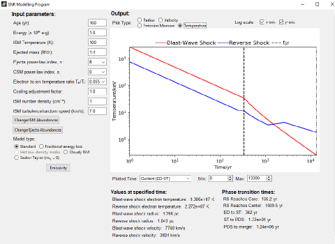
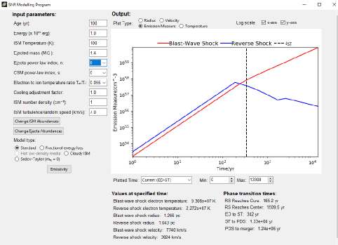
Figure 5: Temperature (top) and Emission Measure (bottom) in physical units as a function of time as calculated by the new software SNRPy. The case shown has s=0, n=8 and other parameters as shown in the screenshot.

The Python code SNR modelling software, SNRPy, was initially presented by LW17. It calculated positions of FS and RS vs. time for several values of s and n from the TM99 solutions, and for the other models described in LW17. The temperatures, emission measures, interior structures and surface brightness profiles were calculated for s=0, n=7 and 12 using the low-resolution published CP solutions, and for low resolution WL91 solutions. A major update to SNRPy has been made as a result of the current work. It now uses the new high resolution CP and WL91 solutions. The new code provides emission measures, interior structure and surface brightness profiles for all values of s=0 and s=2 for all n from 6 to 14 for the self-similar CP phase. For the unified evolution, SNRPy now provides plots of $EM$ and $EM$-weighted $T$ for shocked ISM and shocked ejecta as functions of time. An example of the new calculations is shown in Fig. 5. The new SNRPy code is available for download from the website quarknova.ca in the software section, and from GitHub in repository denisleahy/SNRmodels. The new CP and WL91 structure files are included in the Data directory of SNRPy. The animations of the PLUTO hydro simulations are provided as zip files with SNRPy.

Appendix A Emission Measures (EM) and EM-weighted Temperatures for Self-similar SNR Phases

For completeness, we present dimensionless EMs (dEM) and dimensionless EM-weighted temperatures (dT) for the self-similar phases of SNR evolution. In most cases, these values have not been presented previously in the literature, in part because previous work was primarily concerned with calculations of shock radius and velocity and not with the interior structure required to calculate dEM and dT.

A.1 Pure ST and SNR in cloudy ISM

Following LW17, we refer to the standard ST solution, with zero ejected mass, as ”pure ST” to differentiate it from the ST phases of TM99, with non-zero ejected mass. WL91 present self-similar models for SNR evolution in a cloudy ISM, assuming zero ejected mass.

For simplicity we only consider their one parameter models which depend on $C/\tau$. Here $C=\rho_{c}/\rho_{0}$, with $\rho_{c}$ is the ISM density if the clouds were uniformly dispersed in the ISM and $\rho_{0}$ is the intercloud density prior to cloud evaporation. The evaporation timescale parameter is $\tau=t_{evap}/t$, with $t_{evap}$ the evaporation timescale and $t$ the age of the SNR. The WL91 case $C/\tau=0$ is the same as the pure ST solution.

The WL91 models were recalculated by solving the self-similar differential equations given in WL91, using a variety of differential equation solvers. The equations were solved within both MathCad and Mathematica software packages, using fourth-order Runga-Kutta with adaptive step size, Burlisch-Stoer method, and a hybrid solver which uses a combination of Adams and BDF (backwards differentiation formula). The results were compared and all agreed to 5 digits or better. The solutions agree with the figures shown in WL91.

Results are presented here for $C/\tau$=0 (pure ST), 1, 2 and 4. Fig. 6 shows the interior structure (pressure, density, gas velocity and gas temperature) vs. scaled radius, $r/R_{shock}$. The dimensionless $cEM$ is shown vs. dimensionless impact parameter $b$. The integrated quantities $dEM$ and $dT$ for the WL91 solutions are given in Table 5.

A.2 Early ED Phase

For SNR with non-zero ejected mass, the evolution starts with the early ED phase. The ejecta has a constant density core and power-law density envelope. The self-similar evolution starts at t=0 and ends when the reverse shock approaches the ejecta core (TM99). The self-similar solutions exist for $n>5$ and were discussed by Chevalier (1982). That work presented low resolution interior structure solutions for four cases s=0, n= 7 and 12 and s=2, n=7 and 12. Here we give interior structure solutions, dEM and dT for all values of n= 6 through 14 for both n=0 and s=2.

We calculated the self-similar solutions, labelled CP (Chevalier-Parker) using the methods outlined in Chevalier (1982) and Parker (1963). The equations were solved within both MathCad and Mathematica software packages, using different differential equation solvers, and comparing the results to ensure consistency. The cases s=0 and s=2, for n=6, 7, 8, 9, 10, 11, 12, 13 and 14 were computed.

The s=0 and s=2 solutions for n=7 and n=12 were consistent with those given in Chevalier (1982). Interior solutions for s=0, n=6, 8, 10 and 12 are shown in Fig. 7 for the regions from the reverse shock to the forward shock. Interior solutions for s=2, n=6, 8, 10 and 12 are shown in Fig. 8.

A.3 $EM$s and $EM$-weighted Temperatures

During the self-similar phases of evolution of an SNR, $dEM_{FS}$, $dEM_{RS}$, $dT_{FS}$ and $dT_{RS}$ are constants; $cEM_{FS}(b)$ and $cEM_{RS}(b)$ are functions independent of time. The integrated quantities $dEM$ and $dT$ for the WL solutions for $C/\tau$=0, 1, 2 and 4 are given in Table 5. The dimensionless $cEM$ for the WL solutions are shown as a function of impact parameter $b=B/R_{shock}$ in Fig. 6.

$cEM$ for the CP solutions is shown as a function of $b=B/R_{shock}$ for select s=0 cases in Fig. 9. The $cEM$ for gas between the CD and the FS is shown in the left panel. It varies smoothly with $b$, peaking approximately midway between the CD and the FS because of projection effects. The $cEM$ for gas between the RS and the CD is shown in the right panel. Because the RS-heated gas forms a thinner and much denser shell than FS-heated gas (Fig. 7), the $cEM$ is much more peaked at $b$ between the RS and the CD. Fig. 10 shows $cEM$ vs. $b$ for the s=2 cases. For s=2, both FS-heated gas and RS-heated gas are concentrated in thin and dense shells close to the CD (Fig. 8). In projection, this explains the sharp peak in $cEM$ for both FS-heated gas (left panel) and RS-heated gas (right panel). The extended tail in $cEM$ for $b$ from CD and FS is caused by projection of the low density part of the FS-heated gas.

The integrated quantities $dEM$ and $dT$ from the CP solutions for FS-heated gas and RS-heated gas are given in Table 5. $dEM$ and $dT$ for FS-heated gas varies slowly with n for s=0, whereas for RS-heated gas $dEM$ increases by 2 orders of magnitude and $dT$ decreases by 1 order of magnitude. For s=2 FS-heated gas, $dEM$ increases by a factor of 5 from n=6 to 14 and $dT$ decreases by a factor or 3.5. For s=2 RS-heated gas, $dEM$ increases by 2 orders of magnitude for n=6 to 14, and $dT$ decreases 1 order of magnitude. In summary, for both s=0 and s=2 as n increases from 6 to 14, the RS heated gas is brighter and of lower temperature relative to FS heated gas.

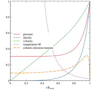
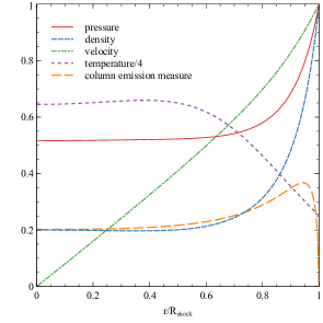
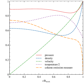
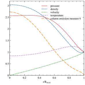
Figure 6: The interior structure of the WL91 self-similar solutions for $C/\tau$=0 (top left), 1 (top right), 2 (bottom left) and 4 (bottom right). The pressure, density, velocity and temperature are plotted vs. radius and are scaled to their values at the forward shock. Further scaling factors are applied to temperature, as noted in the figure legend. The dimensionless column emission measure (long dash line) is plotted vs impact parameter.

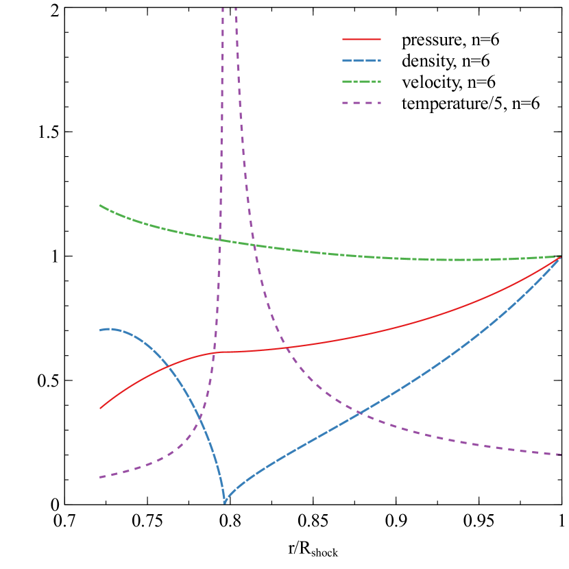
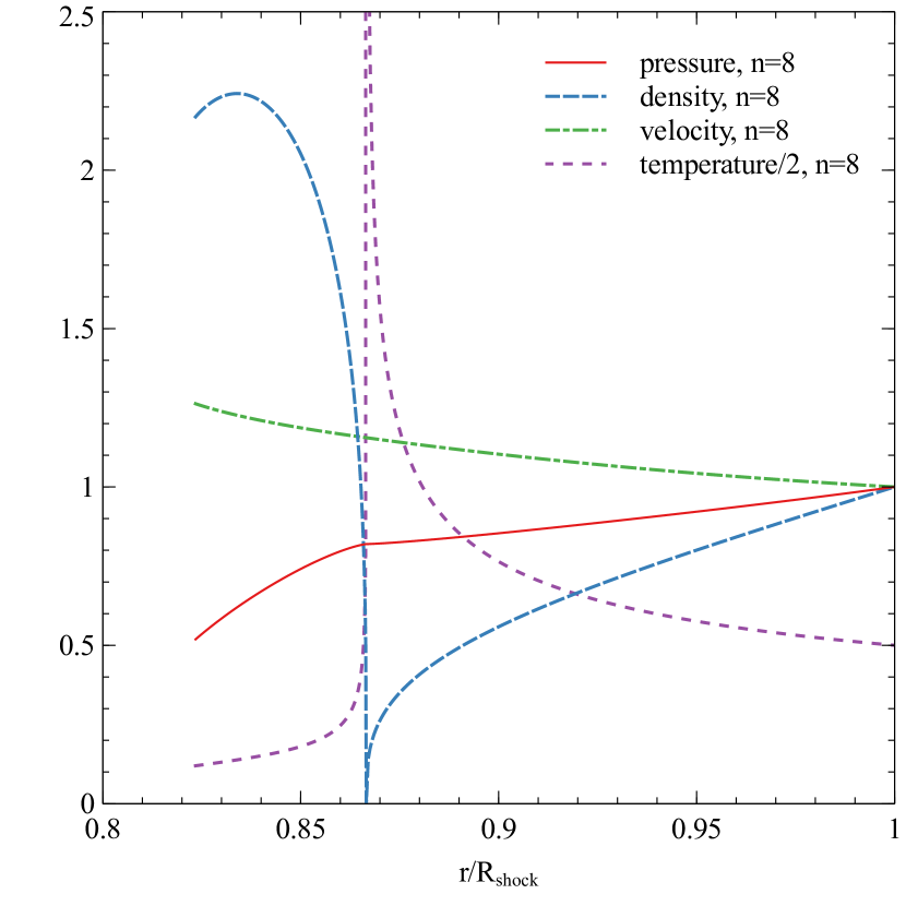
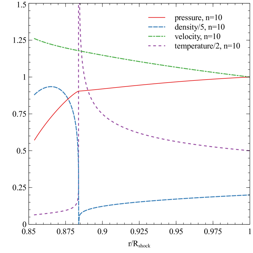
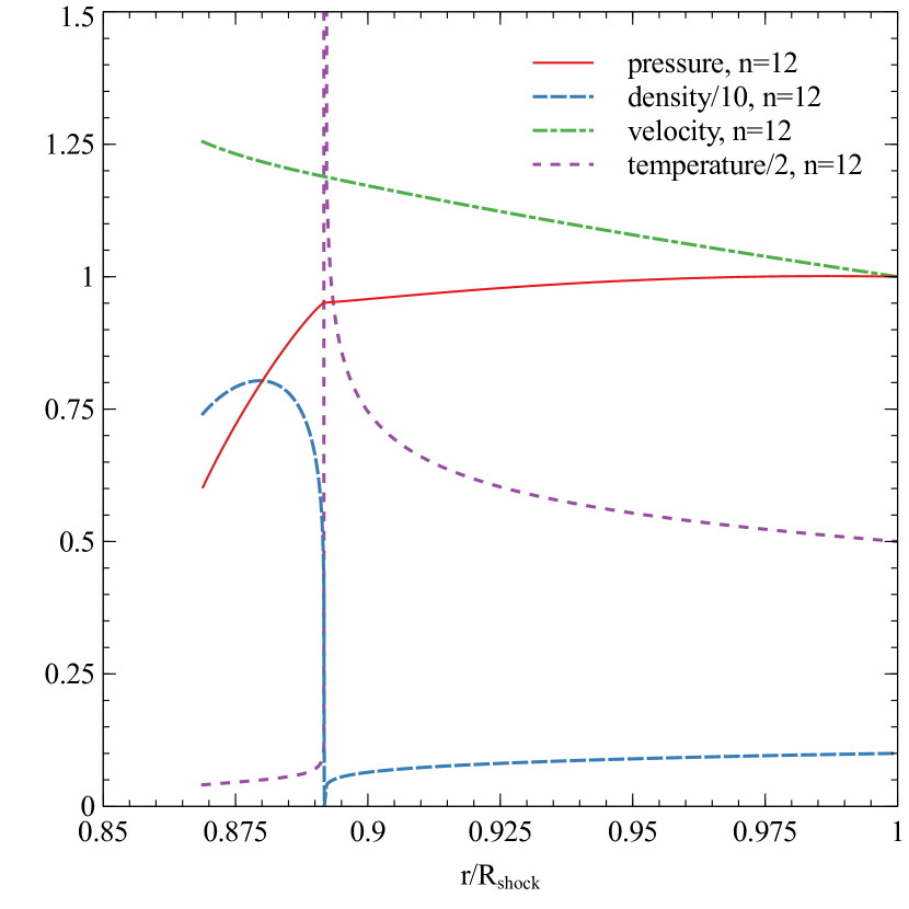
Figure 7: The interior structure of the Chevalier-Parker self-similar solutions for s=0 and n= 6 (top left), 8 (top right), 10 (bottom left), 12 (bottom right). The values are scaled to the post-forward-shock values of pressure, density and temperature and the forward shock velocity. Further scaling factors are applied to density and temperature, as noted in the figure legend. The reverse shock is the point at smallest radius, and the contact discontinuity is where the density goes to zero.

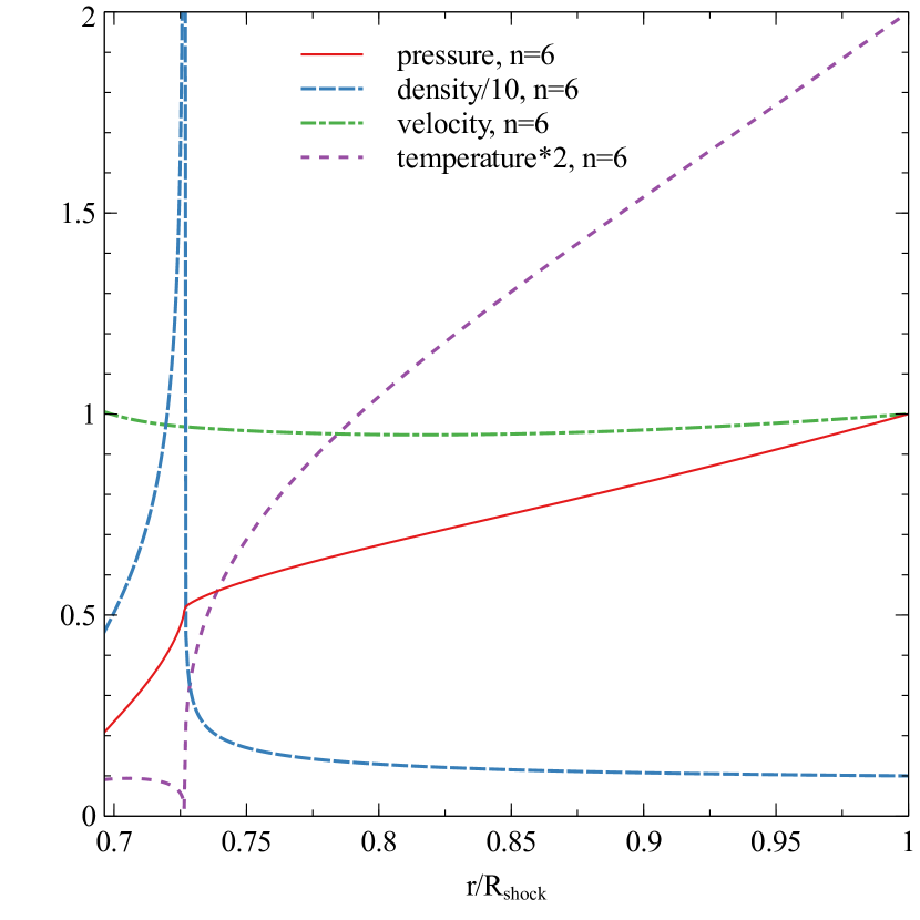
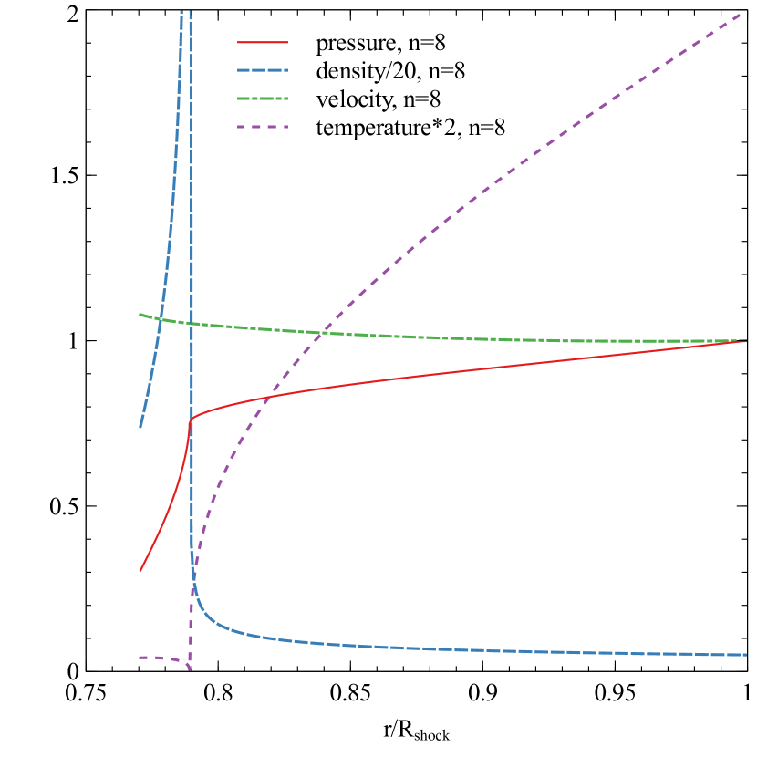
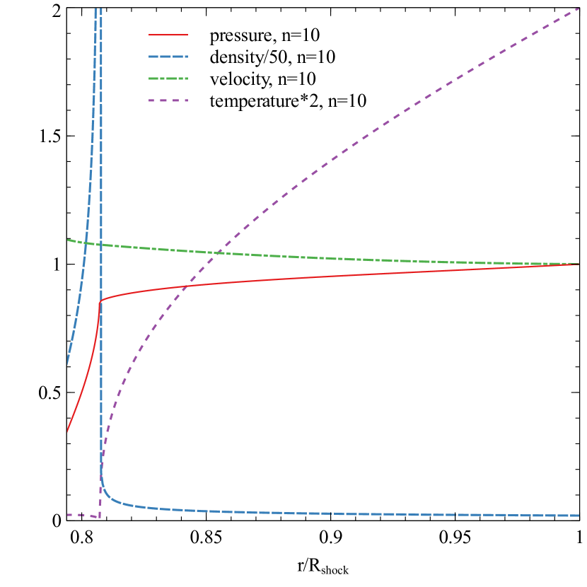
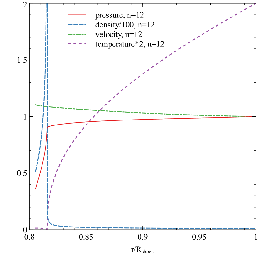
Figure 8: The interior structure of the Chevalier-Parker self-similar solutions for s=2 and n= 6 (top left), 8 (top right), 10 (bottom left), 12 (bottom right). The values are scaled to the post-forward-shock values of pressure, density and temperature and the forward shock velocity. Further scaling factors are applied to density and temperature, as noted in the figure legend. The reverse shock is the point at smallest radius, and the contact discontinuity is where the density goes to infinity.

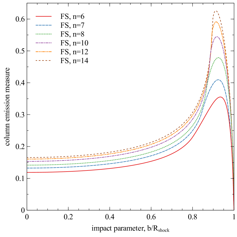
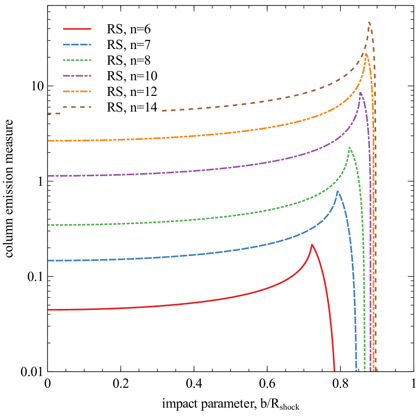
Figure 9: The dimensionless column emission measures vs. impact parameter b for the Chevalier-Parker self-similar solutions for s=0 and n= 6, 7, 8, 10, 12 and 14. The left panel is for material heated by the forward shock, plotted with linear scale. The right panel is for material heated by the reverse shock, plotted with log scale.

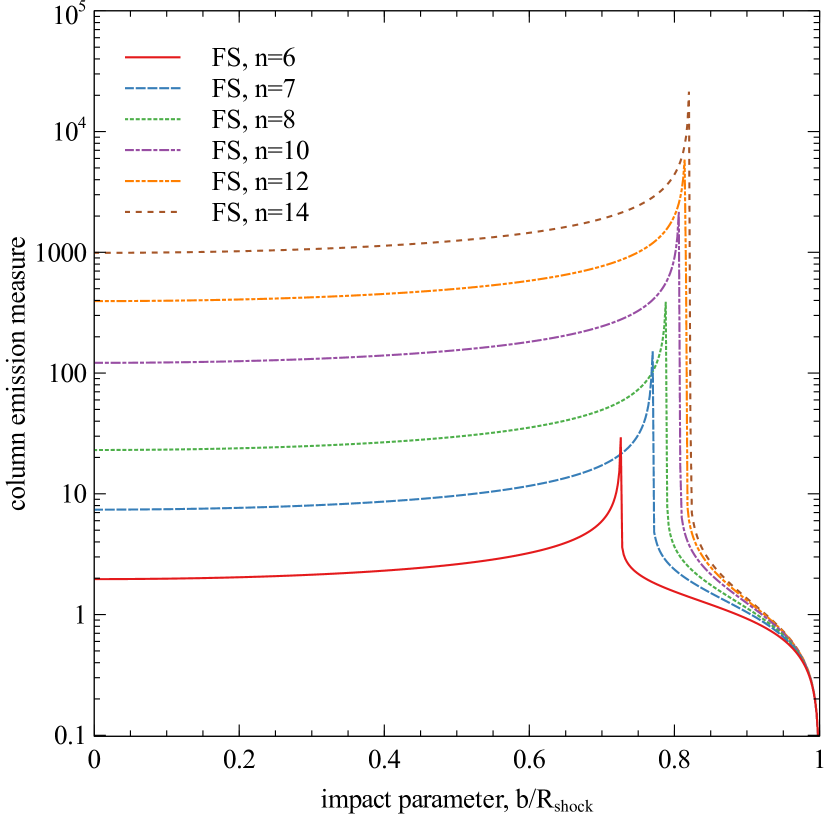
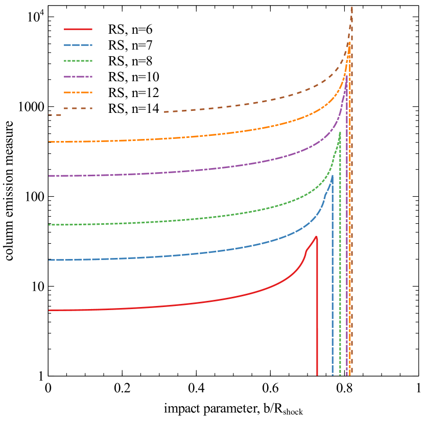
Figure 10: The dimensionless column emission measures vs. impact parameter b for the Chevalier-Parker self-similar solutions for s=2 and n= 6, 7, 8, 10, 12 and 14. The left panel is for material heated by the forward shock and the right panel is for material heated by the reverse shock.

Table 1: Coefficients for Fits to $dT_{FS}(t_{s})$, $dEM_{FS}(t_{s})$, $dT_{RS}(t_{s})$ and $dEM_{RS}(t_{s})$

		n=6	n=7	n=8	n=9	n=10	n=11	n=12	n=13	n=14
$dT_{FS}(t_{s})$	$t_{1}$	0.100	3.011	2.567	0.8303	0.4707	0.4149	0.3158	0.3999	0.2428
	$t_{2}$	1.197	19.43	17.85	11.95	11.24	13.72	11.86	16.48	8.654
	$p_{1}(\times 10^{-2})$	-0.741	2.601	3.346	2.713	2.739	2.805	3.019	3.592	3.594
	$p_{2}(\times 10^{-3})$	0.919	-5.29	-2.43	-0.352	-0.479	-0.285	-0.328	-4.50	-0.322
$dEM_{FS}(t_{s})$	$t_{1}$	0.8058	0.5343	0.4037	0.3352	0.2562	0.2400	0.2083	0.2031	0.1928
	$t_{2}$	2.270	1.762	1.122	1.189	1.247	1.070	1.187	1.194	1.149
	$t_{3}$	9.438	9.785	3.960	8.933	7.256	4.364	6.020	7.464	7.480
	$t_{4}$	45.69	47.79	240.7	40.98	41.69	55.84	51.34	53.16	42.56
	$p_{1}$	-0.2099	-0.2713	-0.3197	-0.3235	-0.2810	-0.2937	-0.2772	-0.2932	-0.2882
	$p_{2}(\times 10^{-2})$	-4.777	-4.595	-11.31	-6.303	-6.753	-10.27	-8.984	-5.229	-7.038
	$p_{3}(\times 10^{-2})$	4.576	5.211	1.795	5.983	4.489	2.715	5.765	3.410	5.166
	$p_{4}(\times 10^{-3})$	$-4.81$	$-6.31$	$-7.08$	$-1.35$	$-0.056$	$-0.572$	$-9.58$	$-0.562$	$-2.12$
$dT_{RS}(t_{s})$	$t_{1}$	0.1001	0.2290	0.4398	0.4016	0.3075	0.2618	0.2382	0.2162	0.1966
	$t_{2}$	1.376	1.229	2.037	2.523	2.686	2.492	2.766	2.801	2.925
	$t_{3}$	5.023	6.995	4.631	4.504	4.520	4.582	4.558	4.508	4.457
	$p_{1}$	-0.0392	0.0782	0.5480	0.6564	0.6537	0.6436	0.6964	0.7265	0.7601
	$p_{2}$	1.264	1.166	1.562	1.842	1.996	1.841	2.094	2.079	2.247
	$p_{3}$	0.7157	0.7137	0.7131	0.7190	0.7159	0.7204	0.7209	0.7211	0.7242
$dEM_{RS}(t_{s})$	$t_{1}$	0.6146	0.4272	0.3382	0.3221	0.2357	0.2209	0.2104	0.1939	0.1747
	$t_{2}$	2.833	2.657	2.953	2.462	2.799	2.832	2.665	2.730	2.681
	$t_{3}$	4.482	4.888	4.513	4.984	4.819	4.861	4.922	4.821	4.848
	$p_{1}$	2.465	2.652	2.733	2.955	2.718	2.781	2.884	2.891	2.882
	$p_{2}$	1.247	1.384	0.781	1.335	1.008	1.023	0.989	1.009	1.006
	$p_{3}$	1.919	1.919	1.919	1.920	1.926	1.927	1.941	1.928	1.933

Table 2: Historical SNR Observed Quantities

SNR	Agea	Type	Distance	Radiusb	EMb,c	kTc	Refsd
	(yr)		(kpc)	(pc)	($10^{58}$cm-3)	(keV)
G$4.5+6.8$ (Kepler)	407	Ia	$5.1^{+0.8}_{-0.7}$	$2.64$d5.1	$0.6007^{+0.0125}_{-0.0202}$d${}_{5.1}^{2}$	$1.06\pm 0.03$	1, 2, 3
G$120.1+1.4$ (Tycho)	$434$	Ia	$4.0\pm 1.0$	4.96d4	$3.421^{+0.144}_{-0.025}$d${}_{4}^{2}$	$0.41\pm 0.01$	4, 5, 3
G$327.6+14.6$ (SN1006)	$1002$	Ia	$2.18\pm 0.08$	9.50d2.18	$0.0485$d${}_{2.18}^{2}$	$0.4\pm 0.1$	6, 7, 8

References. — (1) Kinugasa & Tsunemi (1999), (2) Sankrit et al. (2016), (3) Katsuda et al. (2015), (4) Krause et al. (2008), (5) Hayato et al. (2010), (6) Schaefer (1996), (7) Winkler et al. (2003), (8) Uchida et al. (2013)

Table 3: Historical SNR Shocked Ejecta Quantities

SNR	$EM_{1}^{a}$	$kT_{1}$	$EM_{2}^{a}$	$kT_{2}$	$EM_{3}^{a}$	$kT_{3}$
	($10^{58}$cm-3)	(keV)	($10^{58}$cm-3)	(keV)	($10^{58}$cm-3)	(keV)
Kepler	$2.990^{+0.355}_{-0.031}\times 10^{-5}$	$0.37\pm 0.01$	$2.723^{+0.015}_{-0.013}\times 10^{-5}$	$2.08^{+0.01}_{-0.02}$	$18.07^{+0.22}_{-0.19}\times 10^{-5}$	$2.59\pm 0.01$
Tycho	$17.25^{+0.88}_{-1.48}\times 10^{-5}$	$0.70^{+0.02}_{-0.01}$	$4.353\pm 0.004\times 10^{-7}$	$0.96\pm 0.01$	$2.06\pm 0.2\times 10^{-8}$	$9.34^{+0.03}_{-0.25}$
SN1006	$2.00\times 10^{-6}$	$0.48\pm 0.01$	$5.91\times 10^{-6}$	$1.73\pm 0.03$	$\cdots$	$\cdots$

Table 4: Historical SNR Model Results

SNR	Dist	s	n	$M_{ej}$	Age	Energy	$n_{0}$(s=0)	$\rho_{s}$(s=2)	$\textrm{EM}_{\textrm{RS}}$	$\textrm{kT}_{\textrm{RS}}$	$\textrm{R}_{\textrm{RS}}$
	(kpc)			($M_{\odot}$)	(yr)	($10^{51}$erg)	(cm-3)	(M⊙s/(km yr))	($10^{58}$cm-3)	(keV)	(pc)
G$4.5+6.8$	$5.1$	0	7	1.2	1550	0.0374	0.893	n/a	$1.25\times 10^{-4}$	1.92	2.04
(Kepler)		2	6	1.2	332	0.718	n/a	$4.36\times 10^{-8}$	$2.43\times 10^{-4}$	3.63	1.84
		2	7	1.2	103	5.26	n/a	$1.84\times 10^{-8}$	$1.59\times 10^{-4}$	16.4	1.97
		2	8	1.2	157	2.71	n/a	$2.43\times 10^{-8}$	$6.72\times 10^{-4}$	5.69	2.04
		2	6	1.0	332	0.676	n/a	$4.36\times 10^{-8}$	$2.43\times 10^{-4}$	3.63	1.84
		2	6	1.4	332	0.756	n/a	$4.36\times 10^{-8}$	$2.43\times 10^{-4}$	3.63	1.84
	$4.4$	2	6	1.2	282	0.582	n/a	$3.51\times 10^{-7}$	$1.81\times 10^{-4}$	3.70	1.59
	$5.9$	2	6	1.2	392	0.886	n/a	$5.46\times 10^{-8}$	$3.25\times 10^{-4}$	3.55	2.13
G$120.1+1.4$	$4.0$	0	7	1.2	4050	0.0695	0.967	n/a	$3.10\times 10^{-5}$	1.24	1.32
(Tycho)		2	6	1.2	1830	0.281	n/a	$1.43\times 10^{-7}$	$1.38\times 10^{-3}$	0.59	3.45
		2	7	1.2	378	3.41	n/a	$6.03\times 10^{-8}$	$9.05\times 10^{-4}$	5.41	3.71
		2	8	1.2	688	1.03	n/a	$7.96\times 10^{-8}$	$3.83\times 10^{-3}$	1.52	3.82
		2	7	1.0	378	3.11	n/a	$6.03\times 10^{-8}$	$9.05\times 10^{-4}$	5.41	3.71
		2	7	1.4	378	3.68	n/a	$5.84\times 10^{-8}$	$9.05\times 10^{-4}$	5.41	3.71
	$3.0$	2	7	1.2	278	2.47	n/a	$3.92\times 10^{-8}$	$5.09\times 10^{-4}$	5.50	2.78
	$3.0$	2	8	1.2	498	0.825	n/a	$5.16\times 10^{-8}$	$2.15\times 10^{-3}$	1.58	2.86
	$5.0$	2	7	1.2	480	4.37	n/a	$8.43\times 10^{-8}$	$1.42\times 10^{-3}$	5.33	4.63
G$327.6+14.6$	$2.18$	0	7	1.2	8460	0.0237	0.0394	n/a	$3.61\times 10^{-7}$	0.742	6.66
(SN1006)		2	7	1.2	604	2.75	n/a	$9.94\times 10^{-9}$	$1.28\times 10^{-5}$	6.20	7.10
		2	8	1.2	924	1.32	n/a	$1.31\times 10^{-8}$	$5.43\times 10^{-5}$	2.14	7.32
		2	9	1.2	1140	0.863	n/a	$1.46\times 10^{-8}$	$1.35\times 10^{-4}$	1.13	7.45
		2	8	1.0	924	1.18	n/a	$1.31\times 10^{-8}$	$5.43\times 10^{-5}$	2.14	7.32
		2	8	1.4	924	1.45	n/a	$1.31\times 10^{-8}$	$5.43\times 10^{-5}$	2.14	7.32
	$2.10$	2	9	1.2	1095	0.84	n/a	$1.38\times 10^{-8}$	$1.23\times 10^{-4}$	1.13	7.18
	$2.26$	2	8	1.2	957	1.36	n/a	$1.35\times 10^{-8}$	$5.53\times 10^{-5}$	2.14	7.59

Note. — Type Ia abundances used in this study ($log(\textrm{X/H})+12$)- He: 10.93, O: 12.69, C: 0.0, Ne:12.65, N: 0.0, Mg: 11.96, Si: 12.87, Fe: 13.13, S: 12.52, Ca: 11.97, Ni: 11.85, Na: 6.24, Al: 6.45, Ar: 11.81.

Table 5: Dimensionless Emission Measures and Temperatures for Self-similar Phases

phase	s	n	$C/\tau$	$dEM_{FS}$	$dT_{FS}$	$dEM_{RS}$	$dT_{RS}$
WL91	n/a	n/a	0	0.5164	1.2896	n/a	n/a
	n/a	n/a	1	0.7741	1.3703	n/a	n/a
	n/a	n/a	2	1.6088	1.3693	n/a	n/a
	n/a	n/a	4	6.9322	1.3833	n/a	n/a
CP	0	6	n/a	0.6746	1.2614	0.1604	0.8868
	0	7	n/a	0.7542	1.2227	0.6250	0.5204
	0	8	n/a	0.8081	1.1922	1.549	0.3368
	0	9	n/a	0.8471	1.1694	3.087	0.2347
	0	10	n/a	0.8767	1.1518	5.400	0.1723
	0	11	n/a	0.8998	1.1380	8.634	0.1318
	0	12	n/a	0.9184	1.1270	12.98	0.1039
	0	13	n/a	0.9337	1.1179	18.53	0.0840
	0	14	n/a	0.9465	1.1103	25.50	0.0693
CP	2	6	n/a	17.60	0.1417	12.95	0.0413
	2	7	n/a	99.35	0.0298	47.88	0.0254
	2	8	n/a	56.92	0.0533	116.0	0.0169
	2	9	n/a	45.84	0.0677	227.3	0.0119
	2	10	n/a	62.73	0.0515	391.5	0.00887
	2	11	n/a	79.16	0.0420	619.3	0.00684
	2	12	n/a	94.66	0.0360	920.8	0.00644
	2	13	n/a	75.18	0.0451	1308	0.00442
	2	14	n/a	83.76	0.0411	1788	0.00367

References

- Albinson et al. (1986) Albinson, J. S., Tuffs, R. J., Swinbank, E., et al. 1986, MNRAS, 219, 427
- Badenes et al. (2003) Badenes, C., Bravo, E., Borkowski, K. J., et al. 2003, ApJ, 593, 358
- Badenes et al. (2006) Badenes, C., Borkowski, K. J., Hughes, J. P., et al. 2006, ApJ, 645, 1373
- Borkowski et al. (2001) Borkowski, K. J., Lyerly, W. J., & Reynolds, S. P. 2001, ApJ, 548, 820
- Chevalier (1982) Chevalier, R. A. 1982, ApJ, 258, 790
- Cioffi et al. (1988) Cioffi, D. F., McKee, C. F., & Bertschinger, E. 1988, ApJ, 334, 252
- Cox & Anderson (1982) Cox, D. P., & Anderson, P. R. 1982, ApJ, 253, 268
- Dwarkadas, & Chevalier (1998) Dwarkadas, V. V., & Chevalier, R. A. 1998, ApJ, 497, 807
- Ferrière (2001) Ferrière, K. M. 2001, Reviews of Modern Physics, 73, 1031
- Ghavamian et al. (2013) Ghavamian, P., Schwartz, S. J., Mitchell, J., Masters, A., & Laming, J. M. 2013, Space Sci. Rev., 178, 633
- Green (2014) Green, D. A. 2014, Bulletin of the Astronomical Society of India, 42, 47
- Grevesse & Sauval (1998) Grevesse, N., & Sauval, A. J. 1998, Space Sci. Rev., 85, 161
- Hamilton et al. (1983) Hamilton, A. J. S., Sarazin, C. L., & Chevalier, R. A. 1983, ApJS, 51, 115
- Itoh (1978) Itoh, H. 1978, PASJ, 30, 489
- Hayato et al. (2010) Hayato, A., Yamaguchi, H., Tamagawa, T., et al. 2010, ApJ, 725, 894
- Itoh et al. (2002) Itoh, N., Kawana, Y., & Nozawa, S. 2002, Nuovo Cimento B Serie, 117, 359
- Katsuda et al. (2015) Katsuda, S., Mori, K., Maeda, K., et al. 2015, ApJ, 808, 49
- Kinugasa & Tsunemi (1999) Kinugasa, K., & Tsunemi, H. 1999, PASJ, 51, 239
- Krause et al. (2008) Krause, O., Tanaka, M., Usuda, T., et al. 2008, Nature, 456, 617
- Leahy (2017) Leahy, D. A. 2017, ApJ, 837, 36
- Leahy & Williams (2017) Leahy, D. A., & Williams, J. E. 2017, AJ, 153, 239
- Leahy & Ranasinghe (2018) Leahy, D. A., & Ranasinghe, S. 2018, ApJ, 866, 9
- Liang & Keilty (2000) Liang, E., & Keilty, K. 2000, ApJ, 533, 890
- Maggi et al. (2016) Maggi, P., Haberl, F., Kavanagh, P. J., et al. 2016, A&A, 585, A162
- Martínez-Rodríguez et al. (2018) Martínez-Rodríguez, H., Badenes, C., Lee, S.-H., et al. 2018, ApJ, 865, 151
- Mignone et al. (2007) Mignone, A., Bodo, G., Massaglia, S., et al. 2007, ApJS, 170, 228
- Mignone et al. (2012) Mignone, A., Zanni, C., Tzeferacos, P., et al. 2012, ApJS, 198, 7
- Minkowski (1966) Minkowski, R. 1966, AJ, 71, 371
- Parker (1963) Parker, E. N. 1963, New York, Interscience Publishers, 1963.
- Patnaude et al. (2012) Patnaude, D. J., Badenes, C., Park, S., et al. 2012, ApJ, 756, 6
- Ranasinghe & Leahy (2017) Ranasinghe, S., & Leahy, D. A. 2017, ApJ, 843, 119
- Ranasinghe & Leahy (2018) Ranasinghe, S., & Leahy, D. A. 2018, AJ, 155, 204
- Ranasinghe & Leahy (2018) Ranasinghe, S., & Leahy, D. A. 2018, MNRAS, 477, 2243
- Ranasinghe et al. (2018) Ranasinghe, S., Leahy, D. A., & Tian, W. 2018, Open Physics Journal, 4, 1
- Raymond et al. (1976) Raymond, J. C., Cox, D. P., & Smith, B. W. 1976, ApJ, 204, 290
- Reynoso, & Goss (1999) Reynoso, E. M., & Goss, W. M. 1999, AJ, 118, 926
- Russell & Dopita (1992) Russell, S. C., & Dopita, M. A. 1992, ApJ, 384, 508
- Sankrit et al. (2005) Sankrit, R., Blair, W. P., Delaney, T., et al. 2005, Advances in Space Research, 35, 1027
- Sankrit et al. (2016) Sankrit, R., Raymond, J. C., Blair, W. P., et al. 2016, ApJ, 817, 36
- Schaefer (1996) Schaefer, B. E. 1996, ApJ, 459, 438
- Slane et al. (2014) Slane, P., Lee, S.-H., Ellison, D. C., et al. 2014, ApJ, 783, 33
- Tang & Wang (2005) Tang, S., & Wang, Q. D. 2005, ApJ, 628, 205
- Truelove & McKee (1999) Truelove, J. K., & McKee, C. F. 1999, ApJS, 120, 299
- Uchida et al. (2013) Uchida, H., Yamaguchi, H., & Koyama, K. 2013, ApJ, 771, 56
- Vink (2012) Vink, J. 2012, A&A Rev., 20, 49
- White & Long (1991) White, R. L., & Long, K. S. 1991, ApJ, 373, 543
- Winkler et al. (2003) Winkler, P. F., Gupta, G., & Long, K. S. 2003, ApJ, 585, 324