Capuchin: Causal Database Repair for Algorithmic Fairness

Abstract

Fairness is increasingly recognized as a critical component of machine learning systems. However, it is the underlying data on which these systems are trained that often reflect discrimination, suggesting a database repair problem. Existing treatments of fairness rely on statistical correlations that can be fooled by statistical anomalies, such as Simpson’s paradox. Proposals for causality-based definitions of fairness can correctly model some of these situations, but they require specification of the underlying causal models. In this paper, we formalize the situation as a database repair problem, proving sufficient conditions for fair classifiers in terms of admissible variables as opposed to a complete causal model. We show that these conditions correctly capture subtle fairness violations. We then use these conditions as the basis for database repair algorithms that provide provable fairness guarantees about classifiers trained on their training labels. We evaluate our algorithms on real data, demonstrating improvement over the state of the art on multiple fairness metrics proposed in the literature while retaining high utility.

1 Introduction

In 2014, a team of machine learning experts from Amazon Inc. began work on an automated system to review job applicants’ resumes. According to a recent Reuters article [12], the experimental system gave job candidates scores ranging from one to five and was trained on 10 years of recruiting data from Amazon. However, by 2015 the team realized that the system showed a significant gender bias towards male over female candidates because of historical discrimination in the training data. Amazon edited the system to make it gender agnostic, but there was no guarantee that discrimination did not occur through other means, and the project was totally abandoned in 2017.

Fairness is increasingly recognized as a critical component of machine learning (ML) systems, which make daily decisions that affect people’s lives [11]. The data on which these systems are trained reflect institutionalized discrimination that can be reinforced and legitimized through automation. A naive (and ineffective) approach sometimes used in practice is to simply omit the protected attribute (say, race or gender) when training the classifier. However, since the protected attribute is frequently represented implicitly by some combination of proxy variables, the classifier still learns the discrimination reflected in training data. For example, zip code tends to predict race due to a history of segregation [19, 45]; answers to personality tests identify people with disabilities [4, 52]; and keywords can reveal gender on a resume [12]. As a result, a classifier trained without regard to the protected attribute not only fails to remove discrimination, but it can complicate the detection and mitigation of discrimination downstream via in-processing or post-processing techniques [42, 16, 10, 9, 23, 22, 33, 50], which we next describe.

The two main approaches to reduce or eliminate sources of discrimination are summarized in Fig. 1. The most popular is the in-processing, where the ML algorithm itself is modified; this approach must be reimplemented for every ML application. The alternative is to process either the training data (pre-processing) or the output of the classifier itself (post-processing). We advocate for the pre-processing strategy, which is agnostic to the choice of ML algorithm and instead interprets the problem as a database repair task.

One needs a quantitative measure of discrimination in order to remove it. A large number of fairness definitions have been proposed (see Verma and Rubin for a recent discussion [51]), which we broadly categorize in Fig. 1. The best-known measures are based on associative relationships between the protected attribute and the outcome. For example, Equalized Odds requires that both protected and privileged groups have the same true positive (TP) and false positive (FP) rates. However, it has been shown that associative definitions of fairness can be mutually exclusive [9] and fail to distinguish between discriminatory, non-discriminatory and spurious correlations between a protected attribute and the outcome of an algorithm [22, 33, 13].

Example 1.1

In a well-studied case, UC Berkeley was sued in 1973 for discrimination against females in graduate school admissions when it was found that 34.6% of females were admitted in 1973 as opposed to 44.3% of males. It turned out that females tended to apply to departments with lower overall acceptance rates  [43]. When broken down by department, a slight bias toward female applicant was observed, a result that did not constitute evidence for gender-based discrimination.

Such situations have recently motivated a search for a more principled measure of fairness and discrimination based on causality [22, 33, 23, 16, 42]. These approaches measure the discriminatory causal influence of the protected attribute on the outcome of an algorithm. However, they typically assume access to background information regarding the underlying causal model, which is unrealistic in practice. For example, Kilbertus et al. assume the underlying casual model is provided as a structural equation model [22]. Moreover, no existing proposals describe comprehensive systems for pre-processing data to mitigate causal discrimination.

This paper describes a new approach to removing discrimination by repairing the training data in order to remove the effect of any inappropriate and discriminatory causal relationship between the protected attribute and classifier predictions, without assuming adherence to an underlying causal models.

	Associational	Causal
In-processing	[21, 57, 6, 22]	[33, 22, 42]
(Modify the ML Algorithm)
Pre/post-processing	[14, 7, 17, 54]	Capuchin
(Modify the input/output Data)		(this paper)

Figure 1: Different categories of fairness aware machine-learning methods, based on whether they work with associations/causal definition and whether they modifying algorithm/data to enforce fairness.

Our system, Capuchin, accepts a dataset consisting of a protected attribute (e.g., gender, race, etc.), an outcome attribute (e.g., college admissions, loan application, or hiring decisions), and a set of admissible variables through which it is permissible for the protected attribute to influence the outcome. For example, the applicant’s choice of department in Example 1.1 is considered admissible despite being correlated with gender. The system repairs the input data by inserting or removing tuples, changing the empirical probability distribution to remove the influence of the protected attribute on the outcome through any causal pathway that includes inadmissible attributes. That is, the repaired training data can be seen as a sample from a hypothetical fair world. We make this notion more precise in Section 3.1.

Unlike previous measures of fairness based on causality [33, 22, 42], which require the presence of the underlying causal model, our definition is based solely on the notion of intervention [35] and can be guaranteed even in the absence of causal models. The user need only distinguish admissible and inadmissible attributes; we prove that this information is sufficient to support the causal inferences needed to mitigate discrimination.

We use this interventional approach to derive in Sec. 3.1 a new fairness definition, called justifiable fairness. Justifiable fairness subsumes and improves on several previous definitions and can correctly distinguish fairness violations and non-violations that would otherwise be hidden by statistical coincidences, such as Simpson’s paradox. We prove next, in Sec. 3.2, that, if the training data satisfies a simple saturated conditional independence, then any reasonable algorithm trained on it will be fair.

Our core technical contribution, then, consists of a new approach to repair training data in order to enforce the saturated conditional independence that guarantees fairness. The database repair problem has been extensively studied in the literature [3], but in terms of database constraints, not conditional independence. In Sec. 4 we first define the problem formally and then present a new technique to reduce it to a multivalued functional dependency MVD [1]. Finally, we introduce new techniques to repair a dataset for an MVD by reduction to the MaxSAT and Matrix Factorization problems.

We evaluate our approach in Sec 6 on two real datasets commonly studied in the fairness literature, the adult dataset [26] and the COMPAS recidivism dataset [48]. We find that our algorithms not only capture fairness situations other approaches cannot, but that they outperform the existing state-of-the-art pre-processing approaches even on other fairness metrics for which they were not necessarily designed. Surprisingly, our results show that our repair algorithms can mitigate discrimination as well as prohibitively aggressive approaches, such as dropping all inadmissible variables from the training set, while maintaining high accuracy. For example, our most flexible algorithm, which involves a reduction to MaxSAT, can remove almost 50% of the discrimination while decreasing accuracy by only 1% on adult data.

We make the following contributions:

• We develop a new framework for causal fairness that does not require a complete causal model.

• We prove sufficient conditions for a fair classifier based on this framework.

• We reduce fairness to a database repair problem by linking causal inference to multivalued dependencies (MVDs).

• We develop a set of algorithms for the repair problem for MVDs.

• We evaluate our algorithms on real data and show that they meet our goals and outperform competitive methods on multiple metrics.

Section 2 presents background on fairness and causality, while Section 3 describes sufficient conditions for a fair classifier and derives the database repair problem. In Section 4, we present algorithms for solving the database repair problem and show, in Section 6, experimental evidence that our algorithms outperform the state-of-the-art on multiple fairness metrics while preserving high utility.

Symbol	Meaning
$X,Y,Z$	attributes (variables)
${\mathbf{X}},{\mathbf{Y}},{\mathbf{Z}}$	sets of attributes
$Dom(X),Dom({\mathbf{X}})$	their domains
$x\in Dom(X),{\mathbf{x}}\in Dom({\mathbf{X}})$	a single value, a tuple of values
$D$	the database instance
${\mathbf{V}}$	the attributes of the database $D$
${{{\mathbf{M}}}}=\langle{\mathbf{U}},{\mathbf{V}},{\mathbf{F}},{\tt\mathrm{Pr}}\rangle$	Probabilistic Causal Model (PGM)
$G$	causal DAG
$X\rightarrow Y$	an edge in $G$
${\mathbf{Pa}}(X)$	the parents of $X$ in $G$
${\mathbf{P}}$	a path in $G$
$X\stackrel{{\scriptstyle*}}{{\rightarrow}}Y$	a directed path in $G$
${\mathbf{Z}}\twoheadrightarrow{\mathbf{X}}$	multivalued dependency (MVD)
${\mathbf{X}}\mbox{$\perp\!\!\!\perp$}_{{\tt\mathrm{Pr}}}{\mathbf{Y}}|{\mathbf{Z}}$ or ${\mathbf{X}}\mbox{$\perp\!\!\!\perp$}{\mathbf{Y}}|{\mathbf{Z}}$	conditional independence
$({\mathbf{X}}\mbox{$\perp\!\!\!\perp$}{\mathbf{Y}}|_{d}\ {\mathbf{Z}})$	d-Separation in $G$.
${\bf MB}(X)$	The Markov boundary of $X$
$I$	Inadmissible attributes
$A$	Admissible attributes

Table 1: Notation used in the paper.

2 Preliminaries

We review in this section the basic background on database repair, algorithmic fairness and models of causality, the building blocks of our paper.

The notation used is summarized in Table 1. We denote variables (i.e., dataset attributes) by uppercase letters, $X,Y,Z,$ $V$; their values with lower case letters, $x,y,z,v$; and denote sets of variables or values using boldface (${\mathbf{X}}$ or ${\mathbf{x}}$). The domain of a variable $X$ is $Dom(X)$, and the domain of a set of variables is $Dom({\mathbf{X}})=\prod_{Y\in{\mathbf{X}}}Dom(Y)$. In this paper, all domains are discrete and finite; continuous domains are assumed to be binned, as is typical. A database instance $D$ is a relation whose attributes we denote as ${\mathbf{V}}$. We assume set semantics (i.e., no duplicates) unless otherwise stated, and we denote the cardinality of $D$ as $n=|D|$. Given a partition ${\mathbf{X}}\cup{\mathbf{Y}}\cup{\mathbf{Z}}={\mathbf{V}}$, we say that $D$ satisfies the multivalued dependency (MVD) ${\mathbf{Z}}\twoheadrightarrow{\mathbf{X}}$ if $D=\Pi_{{\mathbf{X}}{\mathbf{Z}}}(D)\Join\Pi_{{\mathbf{Z}}{\mathbf{Y}}}(D)$.

Typically, training data for ML is a bag $B$. We convert it into a set $D$ (by eliminating duplicates) and a probability distribution ${\tt\mathrm{Pr}}$, which accounts for multiplicies; We call $D$ the support of ${\tt\mathrm{Pr}}$. We say that ${\tt\mathrm{Pr}}$ is uniform if all tuples have the same probability. We say ${\mathbf{X}}$ and ${\mathbf{Y}}$ are conditionally independent (CI) given ${\mathbf{Z}}$, written $({\mathbf{X}}\mbox{$\perp\!\!\!\perp$}_{\tt\mathrm{Pr}}{\mathbf{Y}}|{\mathbf{Z}})$, or just $({\mathbf{X}}\mbox{$\perp\!\!\!\perp$}{\mathbf{Y}}|{\mathbf{Z}})$ if ${\tt\mathrm{Pr}}({\mathbf{x}}|{\mathbf{y}},{\mathbf{z}})={\tt\mathrm{Pr}}({\mathbf{x}}|{\mathbf{z}})$ whenever ${\tt\mathrm{Pr}}({\mathbf{y}},{\mathbf{z}})>0$. Conditional independences satisfy the Graphoid axioms [38], which are reviewed in Appendix 8.1 and are used in proofs. When ${\mathbf{V}}={\mathbf{X}}{\mathbf{Y}}{\mathbf{Z}}$, then the CI is said to be saturated. A uniform ${\tt\mathrm{Pr}}$ satisfies a saturated CI iff its support $D$ satisfies the MVD ${\mathbf{Z}}\twoheadrightarrow{\mathbf{X}}$. Training data usually does not have a uniform ${\tt\mathrm{Pr}}$, and in that case the equivalence between the CI and MVD fails [53]; we address this issue in Sec. 4.

The database repair problem is the following: we are given a set of constraints $\Gamma$ and a database instance $D$, and we need to perform a minimal set of updates on $D$ such that the new database $D^{\prime}$ satisfies $\Gamma$ [3]. The problem has been studied extensively in database theory for various classes of constraints $\Gamma$. It is NP-hard even when $D$ consists of a single relation (as it does in our paper) and $\Gamma$ consists of functional dependencies [27]. In our setting, $\Gamma$ consists of conditional independence statements, and it remains NP-hard, as we show in Sec. 4.

2.1 Background on Algorithmic Fairness

Fairness Metric	Description
Demographic Parity (DP) [5]	$S\mbox{$\perp\!\!\!\perp$}O$
a.k.a. Statistical Parity [13]
or Benchmarking [46]
Conditional Statistical parity [10]	$S\mbox{$\perp\!\!\!\perp$}O|{\mathbf{A}}$
Equalized Odds (EO) [17]	$S\mbox{$\perp\!\!\!\perp$}O|Y$
a.k.a. Disparate Mistreatment [56]
Predictive Parity (PP)[9]	$S\mbox{$\perp\!\!\!\perp$}Y|O$
a.k.a. Outcome Test [46]
or Test-fairness [9]
or Calibration [9],
or Matching Conditional Frequencies [17]

Figure 2: Common associational definitions of fairness and their conditional independence statement counterparts.

Algorithmic fairness considers a protected attribute $S$, the response variable $Y$, and a prediction algorithm $A\mathrel{\mathop{\ordinarycolon}}Dom({\mathbf{X}})\rightarrow Dom(O)$, where ${\mathbf{X}}\subseteq{\mathbf{V}}$, whose prediction is denoted $O$ (some references denote it $\tilde{Y}$) and called outcome. For simplicity, we assume $S$ classifies the population into protected $S=1$ and privileged $S=0$, for example, female and male. Fairness definitions can be classified as associational or causal.

Associational fairness

is based on statistical measures on the variables of interest; a summary is shown in Fig. 2. Demographic Parity (DP) [6, 20, 58, 46, 13], requires an algorithm to classify both the protected and the privileged group with the same probability, ${\tt\mathrm{Pr}}(O=1|S=1)={\tt\mathrm{Pr}}(O=1|S=0)$. As we saw in Example 1.1, the lack of statistical parity cannot be considered as evidence for gender-based discrimination; this has motivated the introduction of Conditional Statistical Parity (CSP) [10], which controls for a set of admissible factors ${\mathbf{A}}$, i.e., ${\tt\mathrm{Pr}}(O=1|S=1,{\mathbf{A}}={\mathbf{a}})={\tt\mathrm{Pr}}(O=1|S=0,{\mathbf{A}}={\mathbf{a}})$. Another popular measure used for predictive classification algorithms is Equalized Odds (EO), which requires that both protected and privileged groups to have the same false positive (FP) rate, ${\tt\mathrm{Pr}}(O=1|S=1,Y=0)={\tt\mathrm{Pr}}(O=1|S=0,Y=0)$ , and the same false negative (FN) rate, ${\tt\mathrm{Pr}}(O=0|S=1,Y=1)={\tt\mathrm{Pr}}(O=0|S=0,Y=1)$ Finally, Predictive Parity (PP) requires that both protected and unprotected groups have the same predicted positive value (PPV), ${\tt\mathrm{Pr}}(Y=1|O=i,S=0)={\tt\mathrm{Pr}}(Y=1|O=i,S=1)\ \text{for}\ i,=\{1,0\}$. It has been shown that these measures can be mutually exclusive [9] (see Appendix 8.1).

Causal fairness [23, 22, 33, 42, 16]

was motivated by the need to address difficulties generated by associational fairness and assumes an underlying causal model. We first discuss causal DAGs before reviewing causal fairness.

2.2 Background on Causal DAGs

We now review causal directed acyclic graphs (DAGs) and refer the reader to Appendix 8.1 and [35] for more details.

Causal DAG

A causal DAG $G$ over set of variables ${\mathbf{V}}$ is a directed acyclic graph that models the functional interaction between variables in ${\mathbf{V}}$. Each node $X$ represents a variable in ${\mathbf{V}}$ that is functionally determined by: (a) its parents ${\mathbf{Pa}}(X)$ in the DAG, and (b) some set of exogenous factors that need not appear in the DAG, as long as they are mutually independent. This functional interpretation leads to the same decomposition of the joint probability distribution of ${\mathbf{V}}$ that characterizes Bayesian networks [35]:

$${\tt\mathrm{Pr}}({\mathbf{V}})= \prod_{X\in{\mathbf{V}}}{\tt\mathrm{Pr}}(X|{\mathbf{Pa}}(X))$$ (1)

$d$-Separation and Faithfulness

A common inference question in a causal DAG is how to determine whether a CI $({\mathbf{X}}\mbox{$\perp\!\!\!\perp$}{\mathbf{Y}}|{\mathbf{Z}})$ holds. A sufficient criterion is given by the notion of d-separation, a syntactic condition $({\mathbf{X}}\mbox{$\perp\!\!\!\perp$}{\mathbf{Y}}|_{d}{\mathbf{Z}})$ that can be checked directly on the graph. ${\tt\mathrm{Pr}}$ and $G$ are called Markov compatible if $({\mathbf{X}}\mbox{$\perp\!\!\!\perp$}{\mathbf{Y}}|_{d}{\mathbf{Z}})$ implies $({\mathbf{X}}\mbox{$\perp\!\!\!\perp$}_{\tt\mathrm{Pr}}{\mathbf{Y}}|{\mathbf{Z}})$; if the converse implication holds, then we say that ${\tt\mathrm{Pr}}$ is faithful to $G$. The following is known:

Proposition 2.1

If $G$ is a causal DAG and $\Pr$ is given by Eq.(1), then they are Markov compatible.

(a)

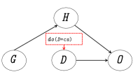
(b)

Figure 3: (a) Represents a causal DAG with $A=$ admission outcome, $G=$ applicant’s gender, $H=$ applicant’s hobbies and $D=$ applicant’s choice of department (cf. Ex. 2.3). (b) Represents the causal DAG obtained after external interventions (cf. Ex. 2.3).

Counterfactuals and do Operator

A counterfactual is an intervention where we actively modify the state of a set of variables ${\mathbf{X}}$ in the real world to some value ${\mathbf{X}}={\mathbf{x}}$ and observe the effect on some output $Y$. Pearl [35] described the $do$ operator that allows this effect to be computed on a causal DAG, denoted ${\tt\mathrm{Pr}}(Y|do(X=x))$. To compute this value, we assume that $X$ is determined by a constant function $X=x$ instead of a function provided by the causal DAG. This assumption corresponds to a modified graph with all edges into ${\mathbf{X}}$ removed, and values of these variables are set to ${\mathbf{x}}$. The Bayesian rule Eq.(1) for the modified graph defines ${\tt\mathrm{Pr}}(Y|do({\mathbf{X}}={\mathbf{x}}))$; the exact expression is in [35, Theorem 3.2.2]. We give an alternative and, to our best knowledge, new formula expressed by introducing some compensating factors; the proof is in Appendix 8.2:

Theorem 2.2

Given a causal DAG $G$ and a set of variables ${\mathbf{X}}\subseteq{\mathbf{V}}$, suppose ${\mathbf{X}}=\{X_{0},X_{1}\ldots X_{m}\}$ are ordered such that $X_{i}$ is a non-descendant of $X_{i+1}$ in $G$. The effect of a set of interventions $do({\mathbf{X}}={\mathbf{x}})$ is given by the following extended adjustment formula:

$${\tt\mathrm{Pr}}(y|do({\mathbf{X}}={\mathbf{x}})) =$$

$$\sum_{{\mathbf{z}}\in Dom({\mathbf{Z}})}{\tt\mathrm{Pr}}(y|{\mathbf{x}},{\mathbf{z}})\bigg{(}\prod_{i=0}^{m}{\tt\mathrm{Pr}}\big{(}{\mathbf{pa}}(X_{i})\bigg{|}\bigcup_{j=0}^{i-1}{\mathbf{pa}}(X_{j}),\bigcup_{j=0}^{i-1}x_{j}\big{)}\bigg{)}$$ (2)

where ${\mathbf{Z}}=\bigcup_{X\in{\mathbf{X}}}{\mathbf{Pa}}(X)$ and $j\geq 0$.

In particular, if ${\mathbf{X}}$ has no parents, then intervention coincides with conditioning, ${\tt\mathrm{Pr}}(y|do({\mathbf{X}}={\mathbf{x}}))={\tt\mathrm{Pr}}(y|{\mathbf{X}}={\mathbf{x}})$.

Example 2.3

Continuing Example 1.1, Fig. 3(a) shows a small fragment of the causal DAG of the admission process in a college. Admissions decisions are made independently by each department and are based on a rich collection of information about the candidates, such as test scores, grades, resumes, statement of purpose, etc. These characteristics affect not only the admission decisions, but also which department the candidate chooses to apply to. We show only a tiny fragment of the causal graph, where $O=$ admission outcome, $D=$ department, $G=$ candidate’s gender, and $H=$ hobbies, which can be influenced by gender. The admissions office anonymizes gender, but it does consider extracurricular activities such as hobbies, so we include an edge $H\rightarrow O$. Since different genders apply to departments at different rates, there is an edge $G\rightarrow D$. Some departments may tend to attract applicants with certain hobbies (e.g., the math department may attract applicants who play chess), so we also include an edge $H\rightarrow D$. The joint distribution is given by

$${\tt\mathrm{Pr}}(g,h,d,o)={\tt\mathrm{Pr}}(g){\tt\mathrm{Pr}}(h|g){\tt\mathrm{Pr}}(d|g,h){\tt\mathrm{Pr}}(o|h,d)$$ (3)

Consider the counterfactual: update the applicant’s department to $cs$. We compare the marginal probability of $O$, the conditional probability, and the intervention:

$${\tt\mathrm{Pr}}(o|D=\text{cs})= \sum_{g,h}{\tt\mathrm{Pr}}(g){\tt\mathrm{Pr}}(h|g){\tt\mathrm{Pr}}(D=\text{cs}|g,h){\tt\mathrm{Pr}}(o|D=\text{cs},h)$$

$${\tt\mathrm{Pr}}(o|do(D=\text{cs}))= \sum_{g,h}{\tt\mathrm{Pr}}(g){\tt\mathrm{Pr}}(h|g){\tt\mathrm{Pr}}(o|D=\text{cs},h)$$ (4)

The expression for intervention (4), based on [35, Theorem 3.2.2] is obtained from the conditional probability by removing the term ${\tt\mathrm{Pr}}(D=\text{cs}|g,h)$, or equivalently deleting the edge $G\rightarrow D$ from the graph in Fig. 3(b). Alternatively, we can express the intervention using Eq.(2) (notice that ${\mathbf{Pa}}(D)=\mathinner{\left\{G,H\right\}}$):

$${\tt\mathrm{Pr}}(o|do(D=\text{cs}))= \sum_{g,h}{\tt\mathrm{Pr}}(o|g,h,D=\text{cs}){\tt\mathrm{Pr}}(h|g){\tt\mathrm{Pr}}(g)$$ (5)

The reader may check that Eq.(4) and (5) are equivalent.

2.3 Causal Fairness

Counterfactual Fairness

Kusner et al. [23, 24] (see also the discussion in [28]) defined a classifier as counterfactually fair if the protected attribute of an individual is not a cause of the outcome of the classifier for that individual, i.e., had the protected attributes of the individual been different, and other things being equal, the outcome of the predictor would have remained the same. However, the definition of counterfactual fairness in [23] captures individual-level fairness only under certain assumptions (see Appendix 8.1). Indeed, it is known in statistics that individual-level counterfactuals can not be estimated from data [39, 40, 41].

Proxy Fairness

To avoid individual-level counterfactuals, a common is to study population-level counterfactuals or interventional distributions that capture the effect of interventions at population level rather than individual level [37, 39, 40]. Kilbertus et. al. [22] defined proxy fairness as follows:

$$P(\tilde{Y}=1|do({\mathbf{P}}={\mathbf{p}}))=P(\tilde{Y}=1|do({\mathbf{P}}={\mathbf{p}}^{\prime}))$$ (6)

for any ${\mathbf{p}},{\mathbf{p}}^{\prime}\in Dom({\mathbf{P}})$, where ${\mathbf{P}}$ consists of proxies to a sensitive variable $S$ (and might include $S$). Intuitively, a classifier satisfies proxy fairness in Eq 6, if the distribution of $\tilde{Y}$ under two interventional regimes in which ${\mathbf{P}}$ set to ${\mathbf{p}}$ and ${\mathbf{p}}^{\prime}$ is the same. Thus, proxy fairness is not an individual-level notion. Next example shows proxy fairness fails to capture group-level discrimination in general.

Example 2.4

To illustrate the difference between counterfactual and proxy fairness, consider the college admission example. Both departments make decisions based on students’ gender and qualifications, $O=f(G,D,Q)$, for a binary $G$ and $Q$. The causal DAG is $G\rightarrow O,D\rightarrow O,Q\rightarrow O$. Let $D=U_{D}$ and $Q=U_{Q}$, where $U_{D}$ and $U_{Q}$ are exogenous factors that are independent and that are uniformly distributed, e.g., $P(U_{Q}=1)=P(U_{Q}=0)=\frac{1}{2}$. Further suppose $f(G,\text{'A'},Q)=G\land Q$ and $f(G,\text{'B'},Q)=(1-G)\land Q$, i.e., dep. A admits only qualified males and dep. B admits only qualified females. This admission process is proxy-fair, because $P(O=1|do(G=1))=P(O=1|do(G=0))=\frac{1}{2}$. On the other hand, it is clearly individually-unfair, in fact it is group-level unfair (for all applicants to the same department). To capture individual fairness, counterfactual fairness [23, 24] is a non-standard definition that does both conditioning and intervention on the sensitive attribute. Conditioning “extracts information from the individual to learn the background variables” [28, pp.11, footnote 1].

Path-specific fairness

These definitions are based on graph properties of the causal graph, e.g., prohibiting specific paths from the sensitive attribute to the outcome [33, 28]; however, identifying path-specific causality from data requires very strong assumptions and is often impractical [2].

3 Defining and Enforcing Algorithmic Fairness

In this section we introduce a new definition of fairness, which, unlike proxy fairness [22], captures correctly group-level fairness, and, unlike counterfactual fairness [23, 24] is based on the standard notion of intervention and, hence, it is testable from the data. In the next section we will describe how to repair an unfair training dataset to enforce fairness.

3.1 Interventional Fairness

This section assumes that the causal graph is given. The algorithm computes an output variable $O$ from input variables ${\mathbf{X}}$ (Sec. 2.1). We begin with a definition describing when an outcome $O$ is causally independent of the protected attribute $S$ for any possible configuration of a given set of variables ${\mathbf{K}}$.

Definition 3.1 (${\mathbf{K}}$-fair)

Fix a set of attributes ${\mathbf{K}}\subseteq{\mathbf{V}}-\mathinner{\left\{S,O\right\}}$. We say that an algorithm $\mathcal{A}\mathrel{\mathop{\ordinarycolon}}Dom({\mathbf{X}})\rightarrow Dom(O)$ is ${\mathbf{K}}$-fair w.r.t. a protected attribute $S$ if, for any context ${\mathbf{K}}={\mathbf{k}}$ and every outcome $O=o$, the following holds:

$${\tt\mathrm{Pr}}(O=o|do(S=0),do({\mathbf{K}}={\mathbf{k}}))={\tt\mathrm{Pr}}(O=o|do(S=1),do({\mathbf{K}}={\mathbf{k}}))$$ (7)

We call an algorithm interventionally fair if it is ${\mathbf{K}}$-fair for every set ${\mathbf{K}}$. Unlike proxy fairness, this notion captures correctly group-level fairness, because it ensures that $S$ does not affect $O$ in any configuration of the system obtained by fixing other variables at some arbitrary values. Unlike counterfactual fairness, it does not attempt to capture fairness at the individual level, and therefore it uses the standard definition of intervention (the do-operator). In fact, we argue that interventional fairness is the strongest notion of fairness that is testable from data, yet captures correctly group-level fairness. We illustrate with an example (see also Ex 3.6).

Example 3.2

In contrast to proxy fairness, interventional fairness correctly identifies the admission process in Ex. 2.4 as unfair at department-level. This is because the admission process fails to satisfy $\mathinner{\left\{D\right\}}$-fairness since, $P(O=1|do(G=0),do(D=\text{'A'}))=0$ but $P(O=1|do(G=1),do(D=\text{'A'}))=\frac{1}{2}$. Therefore, interventional fairness is a more fine-grained notion than proxy fairness. We note however that, interventional fairness does not guarantee individual faintness in general. To see this suppose the admission decisions in both departments are based on student’s gender and an unobserved exogenous factor $U_{O}$ that is uniformly distributed, i.e., $O=f(G,U_{O})$, such that $f(G,0)=G$ and $f(G,1)=1-G$. Hence, the causal DAG is $G\rightarrow O$. Then the admission process is $\emptyset$-fair because, $P(O=1|do(G=1))=P(O=1|do(G=0))=\frac{1}{2}$. Therefore, it is interventionally fair (since ${\mathbf{V}}-\mathinner{\left\{O,G\right\}}=\emptyset$). However, it is clearly unfair at individual level. If the variable $U_{0}$ were endogenous (i.e. known to the algorithm), then the admission process is no longer interventionally fair, because it is not $\mathinner{\left\{U_{o}\right\}}$-fair: $P(O=1|do(G=1),do(U_{o}=1))=P(O=1|G=1,U_{o}=1)=0$, while $P(O=1|do(G=1),do(U_{o}=1))=P(O=1|G=0,U_{o}=1)=1$. Under the same setting counterfactual fairnesses [23, 24] fails to capture individual-level discrimination in this example (see Appendix 8.1).

In practice, interventional fairness is too restrictive, as we show below. To make it practical, we allow the user to classify variables into admissible and inadmissible. The former variables through which it is permissible for the protected attribute to influence the outcome. In Example 1.1, the user would label department as admissible since it is considered a fair use in admissions decisions, and would (implicitly) label all other variables as inadmissible, for example, hobby. Only users can identify this classification, and therefore admissible variables are part of the problem definition:

Definition 3.3 (Fairness application)

A fairness application over a domain ${\mathbf{V}}$ is a tuple $(\mathcal{A},S,{\mathbf{A}},{\mathbf{I}})$, where $\mathcal{A}$ is an algorithm $Dom({\mathbf{X}})\rightarrow Dom(O)$; ${\mathbf{X}}\subseteq{\mathbf{V}}$ are its input variables; $S,O\in{\mathbf{V}}$ are the protected attribute and outcome, and ${\mathbf{A}}\cup{\mathbf{I}}={\mathbf{V}}-\mathinner{\left\{S,O\right\}}$ is a partition of the variables into admissible and inadmissible.

We can now introduce our definition of fairness:

Definition 3.4 (Justifiable fairness)

A fairness application $(\mathcal{A},$ $S,{\mathbf{A}},{\mathbf{I}})$ is justifiability fair if it is ${\mathbf{K}}$-fair w.r.t. all supersets ${\mathbf{K}}\supseteq{\mathbf{A}}$.

Notice that interventional fairness corresponds to the case where no variable is admissible, i.e., ${\mathbf{A}}=\emptyset$.

We give next a characterization of justifiable fairness in terms of the structure of the causal DAG:

Theorem 3.5

If all directed paths from $S$ to $O$ go through an admissible attribute in ${\mathbf{A}}$, then the algorithm is justifiably fair. If the probability distribution is faithful to the causal DAG, then the converse also holds.

To ensure interventional fairness, a sufficient condition is that there exists no path from $S$ to $O$ in the causal graph (because ${\mathbf{A}}=\emptyset$). (Hence, under faithfulness, interventional fairness implies fairness at individual-level, i.e., intervening on the sensitive attribute does not change the counterfactual outcome of individuals.) Since this is too strong in most scenarios, we adopt justifiable fairness instead.

(a) College I

(b) College II

College I	Dept. A		Dept. B		Total
	Admitted	Applied	Admitted	Applied	Admitted	Applied
Male	16	20	16	80	32	100
Female	16	80	16	20	32	100

College  II	Dept. A		Dept. B		Total
	Admitted	Applied	Admitted	Applied	Admitted	Applied
Male	10	10	40	90	50	100
Female	40	50	10	50	50	100

Figure 4: Admission process representation in two colleges where the associational notions of fairness fail (see Ex.3.6).

We illustrate with an example.

Example 3.6

Fig 4 shows how fair or unfair situations may be hidden by coincidences but exposed through causal analysis. In both examples, the protected attribute is gender $G$, and the admissible attribute is department $D$. Suppose both departments in College I are admitting only on the basis of their applicants’ hobbies. Clearly, the admission process is discriminatory in this college because department A admits 80% of its male applicants and 20% of the female applicants, while department B admits 20% of male and 80% of female applicants. On the other hand, the admission rate for the entire college is the same 32% for both male and female applicants, falsely suggesting that the college is fair. Suppose $H$ is a proxy to $G$ such that $H=G$ ($G$ and $H$ are the same), then proxy fairness classifies this example as fair: indeed, since Gender has no parents in the causal graph, intervention is the same as conditioning, hence ${\tt\mathrm{Pr}}(O=1|do(G=\text{i}))={\tt\mathrm{Pr}}(O=1|G=\text{i})$ for $i=0,1$. Of the previous methods, only conditional statistical parity correctly indicates discrimination. We illustrate how our definition correctly classifies this examples as unfair. Indeed, assuming the user labels the department $D$ as admissible, $\mathinner{\left\{D\right\}}$-fairness fails because, by Eq.(2), ${\tt\mathrm{Pr}}(O=1|do(G=1),do(D=\text{'A'}))=\sum_{h}{\tt\mathrm{Pr}}(O=1|G=1,D=\text{'A'},h){\tt\mathrm{Pr}}(h|G=1)={\tt\mathrm{Pr}}(O=1|G=1,D=\text{'A'})=0.8$, and, similarly ${\tt\mathrm{Pr}}(O=1|do(G=0),do(D=\text{'A'}))=0.2$. Therefore, the admission process is not justifiably fair.

Now, consider the second table for College II, where both departments A and B admit only on the basis of student qualifications $Q$. A superficial examination of the data suggests that the admission is unfair: department A admits 80% of all females, and 100% of all male applicants; department B admits 20% and 44.4% respectively. Upon deeper examination of the causal DAG, we can see that the admission process is justifiably fair because the only path from Gender to the Outcome goes through department, which is an admissible attribute. To understand how the data could have resulted from this causal graph, suppose 50% of each gender have high qualifications and are admitted, while others are rejected, and that 50% of females apply to each department but more qualified females apply to department A than to B (80% v.s. 20%). Further, suppose fewer males apply to department A, but all of them are qualified. The algorithm satisfies demographic parity and proxy fairness but fails to satisfy conditional statistical parity since ${\tt\mathrm{Pr}}(A=1|G=1,D=\text{A})=0.8$ but ${\tt\mathrm{Pr}}(A=1|G=0,D=\text{A})=0.2)$. Thus, conditioning on $D$ falsely indicates discrimination in College II. One can check that the algorithm is justifiably fair, and thus our definition also correctly classifies this example; for example, $\mathinner{\left\{D\right\}}$-fairness follows from Eq.(2): ${\tt\mathrm{Pr}}(O=1|do(\text{G}=\text{i}),do(D=d))=\sum_{q}{\tt\mathrm{Pr}}(O=1|G=i,d,q)){\tt\mathrm{Pr}}(q|G=i)=\frac{1}{2}$. To summarize, unlike previous definitions of fairness, justifiable fairness correctly identifies College I as discriminatory and College II as fair.

3.2 Testing Fairness on the Training Data

In this section we introduce a sufficient condition for testing justifiable fairness, which uses only the training data $D,{\tt\mathrm{Pr}}$ (Sec. 2) and does not require access to the causal graph $G$. We assume only that $G$ and ${\tt\mathrm{Pr}}$ are Markov compatible (Sec. 2.2). The training data has an additional response variable $Y$. As before, we assume a fairness application $(\mathcal{A},$ $S,{\mathbf{A}},{\mathbf{I}})$ is given and that the algorithm is a good prediction of the response variable, i.e.  ${\tt\mathrm{Pr}}(Y=1|{\mathbf{X}}={\mathbf{x}})\approx{\tt\mathrm{Pr}}(O=1|{\mathbf{X}}={\mathbf{x}})$; we call the algorithm a reasonable classifier to indicate that it satisfies this condition. Note that this is a typical assumption in pre-processing approachs, see e.g., [7] and needed to decouple the the issues of model accuracy and fairness. If the distributions of ${\tt\mathrm{Pr}}(Y=1|{\mathbf{X}}={\mathbf{x}})$ and ${\tt\mathrm{Pr}}(O=1|{\mathbf{X}}={\mathbf{x}})$ could be arbitrarily far apart, no fairness claims can be made about a classifier that, for example, imposes a pre-determined distribution on the outcome predictions rather than learning an approximation of ${\tt\mathrm{Pr}}(Y=1|{\mathbf{X}}={\mathbf{x}})$ from the training data.

We first establish a technical condition for fairness based on the Markov boundary, and then we simplify it. Recall that, give a probability distribution $\Pr$, the Markov boundary of a variable $Y\in{\mathbf{V}}$, denoted ${\bf MB}(Y)$, is a minimal subset of ${\mathbf{V}}-\mathinner{\left\{Y\right\}}$ that satisfies the saturated conditional independence $(Y\mbox{$\perp\!\!\!\perp$}_{\tt\mathrm{Pr}}{\mathbf{V}}-({\bf MB}(Y)\cup\mathinner{\left\{Y\right\}})|{\bf MB}(Y))$. Intuitively, ${\bf MB}(Y)$ shields $Y$ from the influence of other variables. It is usually assumed that the Markov boundary of a variable is unique (see Appendix 8.1). We prove:

Theorem 3.7

A sufficient condition for a fairness application $(\mathcal{A},S,{\mathbf{A}},{\mathbf{I}})$ to be justifiably fair is ${\bf MB}(O)\subseteq{\mathbf{A}}$.

If ${\tt\mathrm{Pr}}$ is faithful to the causal graph, then the theorem follows immediately from Theorem 3.5; but we prove it without assuming faithfulness in Appendix 8.2. The condition in Theorem 3.7 can be checked without knowing the causal DAG, but requires the computation of the Markov boundary; moreover, it is expressed in terms of the outcome $O$ of the algorithm. We derive from here a sufficient condition without reference to the Markov boundary, which refers only to the response variable $Y$ present in the training data.

Corollary 3.8

Fix a training data $D,{\tt\mathrm{Pr}}$, where $Y\in{\mathbf{V}}$ is the training label, and ${\mathbf{A}},{\mathbf{I}}$ are admissible and inadmissible attributes. Then any reasonable classifier trained on a set of variables ${\mathbf{X}}\subseteq{\mathbf{V}}$ is justifiably fair w.r.t. a protected attribute $S$, if any of the following hold:

• ${\tt\mathrm{Pr}}$ satisfies the CI $(Y\mbox{$\perp\!\!\!\perp$}{\mathbf{X}}\cap{\mathbf{I}}|{\mathbf{X}}\cap{\mathbf{A}})$, or

• ${\mathbf{X}}\supseteq{\mathbf{A}}$ and ${\tt\mathrm{Pr}}$ satisfies the saturated CI $(Y\mbox{$\perp\!\!\!\perp$}{\mathbf{{\mathbf{missing}}}}I|{\mathbf{A}})$.

The proof is the Appendix. While condition (a) is the weaker assumption, condition (b) has the advantage that the CI is saturated. Our method for building a fair classifier is to repair the training data in order to enforce (b).

3.3 Building Fair Classifiers

This leads us to the following methods for building justifiably fair classifiers.

Dropping Inadmissible Attributes

A naive way to satisfy Corollary 3.8(a) is to set ${\mathbf{X}}={\mathbf{A}}$, in other words to train the classifier only on admissible attributes This method guarantees fairness, but, as we will show in Sec. 6, dropping even one inadmissible variable can negatively affect the accuracy of the classifier. Moreover, this approach cannot be used in data release situations, where all variables must be included. Releasing data that reflect discrimination can unintentionally reinforce and amplify discrimination in other contexts that data is used.

Repairing Training Data

Instead, our approach is to repair the training data to enforce the condition in Corollary 3.8(b). We consider the saturated CI $(Y\mbox{$\perp\!\!\!\perp$}{\mathbf{I}}|{\mathbf{A}})$ as an integrity constraint that should always hold in training data $D,{\tt\mathrm{Pr}}$. Capuchin performs a sequence of database updates (viz., insertions and deletions of tuples) to obtain another training database $D^{\prime}$ to satisfy $(Y\mbox{$\perp\!\!\!\perp$}{\mathbf{I}}|{\mathbf{A}})$. We describe this repair problem in Sec. 4. To the causal DAG, this approach can be seen as modifying the underlying causal model to enforce the fairness constraint. However, instead of intervening on the causal DAG, which we do not know and over which we have no control, we intervene on the training data to ensure fairness. Note that minimal repairs are crucial for preserving the utility of data. Specifically, we need to ensure that the joint distribution of training and repaired data are close. Since there is no general metric to measure the distance between two distributions that works well for all datasets and applications, in Sec 4 we propose several minimal repair methods. We empirically show that these methods behave differently for different datasets and ML algorithms. We also note that the negative effect of repair on utility depends on several factors such as the size of data, sparsity of data, repair method, ML algorithm, strongness of dependency that the repair method enforces; hence accuracy should be trade with fairness at training time.

4 Repairing Training Data to Ensure Fairness

We have shown in Corollary 3.8 that, if the training data $D$ satisfies a certain saturated conditional independence (CI), then a classification algorithm trained on $D,{\tt\mathrm{Pr}}$ is justifiably fair. We show here how to modify (repair) the training data to enforce the CI and thus ensure that any reasonable classifier trained on it will be justifiably fair.

4.1 Minimal Repair for MVD and CI

We first consider repairing an MVD. Fix an MVD ${\mathbf{Z}}\twoheadrightarrow{\mathbf{X}}$ and a database $D$ that does not satisfy it. The minimal database repair problem is this: find another database $D^{\prime}$ that satisfies the MVD such that the distance between $D$ and $D^{\prime}$ is minimized. In this section, we restrict the distance function to the symmetric difference, i.e, $|\Delta(D,D^{\prime})|$.

D: X Y Z $${\tt\mathrm{Pr}}$$

$$D_{1}\mathrel{\mathop{\ordinarycolon}}$$ X Y Z

$$D_{2}\mathrel{\mathop{\ordinarycolon}}$$ X Y Z

Figure 5: A simple database repair: $D$ does not satisfy the MVD $Z\twoheadrightarrow X$. In $D_{1}$, we inserted the tuple $(b,b,c)$ to satisfy the MVD, and in $D_{2}$ we deleted the tuple $(b,a,c)$ to satisfy the MVD.

Example 4.1

Consider the database $D$ in Fig. 5 (ignoring the probabilities for the moment), and the MVD $Z\twoheadrightarrow X$. $D$ does not satisfy the MVD. The figure shows two minimal repairs, $D_{1},D_{2}$, one obtained by inserting a tuple, and the other by deleting a tuple.

However, our problem is to repair for a saturated CI, not an MVD, since that is what is required in Corollary 3.8. The repair problem for a database constraint is well-studied in the literature, but here we need to repair to satisfy a CI, which is not a database constraint. We first formally define the repair problem for a CI then show how to reduce it to the repair for an MVD. More precisely, our input is a database $D$ and a probability distribution $\Pr$, and the goal is to define a “repair” $D^{\prime},{\tt\mathrm{Pr}}^{\prime}$ that satisfies the given CI.

We assume that all probabilities are rational numbers. Let the bag associated to $D,{\tt\mathrm{Pr}}$ to be the smallest bag $B$ such that ${\tt\mathrm{Pr}}$ is the empirical distribution on $B$. In other words, $B$ is obtained by replicating each tuple $t\in D$ a number of times proportional to ${\tt\mathrm{Pr}}(t)$. If ${\tt\mathrm{Pr}}$ is uniform, then $B=D$.

Definition 4.2

The minimal repair of $D,{\tt\mathrm{Pr}}$ for a saturated CI $({\mathbf{X}};{\mathbf{Y}}|{\mathbf{Z}})$ is a pair $D^{\prime},{\tt\mathrm{Pr}}^{\prime}$ such that ${\tt\mathrm{Pr}}^{\prime}$ satisfies the CI and $|\Delta(B,B^{\prime})|$ is minimized, where $B$ and $B^{\prime}$ are the bags associated to $D,{\tt\mathrm{Pr}}$ and $D^{\prime},{\tt\mathrm{Pr}}^{\prime}$, respectively.

Recall that ${\mathbf{V}}$ denotes the set of attributes of $D$. Let ${\tt\mathrm{Pr}}$ be any probability distribution on the variables $\mathinner{\left\{K\right\}}\cup{\mathbf{V}}$, where $K$ is a fresh variable not in ${\mathbf{V}}$.

Lemma 4.3

If ${\tt\mathrm{Pr}}$ satisfies $(K{\mathbf{X}};{\mathbf{Y}}|{\mathbf{Z}})$, then it also satisfies $({\mathbf{X}};{\mathbf{Y}}|{\mathbf{Z}})$.

The lemma follows immediately from the Decomposition axiom in Graphoid (see Appendix 8.1).

We now describe our method for computing a minimal repair of $D,{\tt\mathrm{Pr}}$ for some saturated CI. First, we compute the bag $B$ associated to $D,{\tt\mathrm{Pr}}$. Next, we add the new attribute $K$ to the tuples in $B$ and assign distinct values to $t.K$ to all duplicate tuples $t$, thus converting $B$ into a set $D_{B}$ with attributes $K\cup{\mathbf{V}}$. Importantly, we use as few distinct values for $K$ as possible, i.e., we enumerate the instances of each unique tuple. More precisely, we define:

$$D_{B}=\mathinner{\left\{(i,t)|t\in B,i=1,\ldots,|t_{B}|\right\}}$$ (8)

were $|t_{B}|$ denotes the number of occurrences (or multiplicity) of a tuple $t$ in the bag $B$. Then, we repair $D_{B}$ w.r.t. to the MVD ${\mathbf{Z}}\twoheadrightarrow K{\mathbf{X}}$, obtaining a repaired database $D_{B}^{\prime}$. Finally, we construct a new training set $D^{\prime}=\Pi_{{\mathbf{V}}}(D_{B}^{\prime})$, with the probability distribution obtained by marginalizing the empirical distribution on $D_{B}^{\prime}$ to the variables ${\mathbf{V}}$. We prove the following:

Theorem 4.4

Let $D$ be a database and ${\tt\mathrm{Pr}}$ a probability distribution on its tuples, and let $B$ be the associated bag (with attributes $\mathinner{\left\{K\right\}}\cup{\mathbf{V}}$). Fix a saturated CI $({\mathbf{X}};{\mathbf{Y}}|{\mathbf{Z}})$, and let $B^{\prime}$ be a minimal repair for the MVD ${\mathbf{Z}}\twoheadrightarrow K{\mathbf{X}}$. Then, $D^{\prime},{\tt\mathrm{Pr}}^{\prime}$ is a minimal repair of $D,{\tt\mathrm{Pr}}$ for the CI, where $D^{\prime}$ is $B^{\prime}$ with duplicates removed, and ${\tt\mathrm{Pr}}^{\prime}$ is the empirical distribution on $B^{\prime}$.

We illustrate with an example.

B: X Y Z

$$a$$

$$D_{B}\mathrel{\mathop{\ordinarycolon}}$$ K X Y Z

1

2

3

1

2

1

2

1

$$D^{\prime}_{B}\mathrel{\mathop{\ordinarycolon}}$$ K X Y Z

1

2

1

2

1

1

1

$$D^{\prime}\mathrel{\mathop{\ordinarycolon}}$$ X Y Z

Figure 6: Repairing a conditional independence (CI).

Example 4.5

In Example 4.1 we showed two repairs $D_{1},D_{2}$ of the database $D$ in Fig 5 for the MVD $Z\twoheadrightarrow X$. Consider now the probability distribution, ${\tt\mathrm{Pr}}$ shown in the figure. Suppose we want to repair it for the CI $(X;Y|Z)$. Clearly, both $D_{1}$ and $D_{2}$, when endowed with the empirical distribution do satisfy this CI, but they are very poor repairs because they completely ignore the probabilities in the original training data, which are important signals for learning. Our definition captures this by insisting that the repaired bag $B^{\prime}$ be close to the bag $B$ associated to $D,{\tt\mathrm{Pr}}$ (see $B$ in Fig. 6), but the sets $D_{1}$ and $D_{2}$ are rather far from $B$. Instead, our method first converts $B$ into a set $D_{B}$ by adding a new attribute $K$ (see Fig. 6) then, it repairs $D_{B}$ for the MVD $Z\twoheadrightarrow KX$, obtaining $D_{B}^{\prime}$. The final repair $D^{\prime},{\tt\mathrm{Pr}}^{\prime}$ consists of the empirical distribution on $D_{B}^{\prime}$, but with the attribute $K$ and duplicates removed.

We note that, in order for Theorem 4.4 to hold, it is critical that we use minimum distinct values for the attribute $K$ in $D_{B}$; otherwise minimal repairs of $D_{B}$ are no longer minimal repairs of the original data $D,{\tt\mathrm{Pr}}^{\prime}$. For example, if we use distinct values for $K$, thus making $K$ a key, then only subset of $D_{B}$ that satisfies the MVD ${\mathbf{Z}}\twoheadrightarrow K{\mathbf{X}}$ is the empty set.

4.2 Reducing Minimal Repair to 3SAT

Corollary 3.8 requires us to repair the training data $D$ to satisfy a CI. We have shown how to convert this problem into the problem of repairing a derived data $D_{B}$ to satisfy an MVD. In this section we describe how to find a minimal repair for an MVD by reduction to the weighted MaxSAT problem.

We denote the database by $D$, the MVD by $\varphi\mathrel{\mathop{\ordinarycolon}}{\mathbf{Z}}\twoheadrightarrow{\mathbf{X}}$, and assume that $D$’s attributes are ${\mathbf{V}}={\mathbf{X}}\cup{\mathbf{Y}}\cup{\mathbf{Z}}$. Recall that $D$ satisfies the MVD iff $D=\Pi_{{\mathbf{X}}{\mathbf{Z}}}(D)\Join\Pi_{{\mathbf{Y}}{\mathbf{Z}}}(D)$. Since we want to allow repairs that include both insertions and deletions, we start by finding an upper bound on the set of tuples that we may want to insert in the database. For example, one can restrict the set of tuples to those that have only constants that already occurring in the database, i.e., an upper bound is $ADom^{k}$, where $ADom$ is the active domain of $D$, and $k$ is the arity of $D$. However, this set is too large in practice. Instead, we prove that it suffices to consider candidate tuples in a much smaller set, given by: $D^{*}\stackrel{{\scriptstyle\text{def}}}{{=}}\Pi_{{\mathbf{X}}{\mathbf{Z}}}(D)\Join\Pi_{{\mathbf{Z}}{\mathbf{Y}}}(D)$.

Proposition 4.6

Any minimal repair $D^{\prime}$ of $D$ for an MVD satisfies $D^{\prime}\subseteq D^{*}$.

Next, we associate the following Boolean Conjunctive query to the MVD $\varphi$:

$$Q_{\varphi}\leftarrow\ D({\mathbf{X}}_{1},{\mathbf{Y}}_{1},{\mathbf{Z}}),D({\mathbf{X}}_{2},{\mathbf{Y}}_{2},{\mathbf{Z}}),\neg D({\mathbf{X}}_{1},{\mathbf{Y}}_{2},{\mathbf{Z}})$$ (9)

It follows immediately that $D\not\models\varphi$ iff $D\models Q_{\varphi}$, and therefore the repair problem becomes: modify the database $D$ to make $Q_{\varphi}$ false. For that purpose, we use the lineage of the query $Q_{\varphi}$. By the previous proposition, we know that we need to consider as candidates for insertions only those tuples in $D^{*}$; hence we compute the lineage over the set of possible tuples $D^{*}$. We briefly review here the construction of the lineage and refer the reader to [55] and the references there for more detail. We associate a distinct Boolean variable $X_{t}$ to each tuple $t\in D^{*}$, and consider all mappings $\theta\mathrel{\mathop{\ordinarycolon}}Var(Q_{\varphi})\rightarrow ADom(D)$ such that each of the three tuples– $D^{*}(\theta(X_{1}),\theta(Y_{1}),\theta(Z)),D^{*}(\theta(X_{2}),\theta(Y_{2}),\theta(Z))$, and $D^{*}(\theta(X_{1}),$ $\theta(Y_{2}),\theta(Z))$– are in $D^{*}$. Then, the lineage and its negation are:

$$\Phi_{\varphi}= \bigvee_{\theta}\left(X_{D^{*}(\theta(X_{1}),\theta(Y_{1}),\theta(Z))}\land X_{D^{*}(\theta(X_{2}),\theta(Y_{2}),\theta(Z))}\land\neg X_{D^{*}(\theta(X_{1}),\theta(Y_{2}),\theta(Z))}\right)$$ (10)

$$\neg\Phi_{\varphi}= \bigwedge_{\theta}\left(\neg X_{D^{*}(\theta(X_{1}),\theta(Y_{1}),\theta(Z))}\lor\neg X_{D^{*}(\theta(X_{2}),\theta(Y_{2}),\theta(Z))}\lor X_{D^{*}(\theta(X_{1}),\theta(Y_{2}),\theta(Z))}\right)$$ (11)

Recall that an assignment is a mapping from Boolean variables $X_{t}$ to $\mathinner{\left\{0,1\right\}}$. Thus, our goal is to find an assignment satisfying the 3CNF $\neg\Phi_{\varphi}$, which is as close as possible to the initial assignment $X_{t}=1$ for $t\in D$, $X_{t}=0$ for $t\in D^{*}-D$.

We briefly review the weighted MaxSAT problem here. Its input is a 3CNF ${\mathbf{F}}$ whose clauses are partitioned into ${\mathbf{F}}=({\mathbf{F}}_{h},{\mathbf{F}}_{s},\mathcal{C})$, where ${\mathbf{F}}_{h}$ are called the hard clauses, and ${\mathbf{F}}_{s}$ are the soft clauses, and a function ${\mathbf{C}}\mathrel{\mathop{\ordinarycolon}}{\mathbf{F}}_{s}\rightarrow R^{+}$ associates a non-negative cost with each soft clause. A solution to the problem finds an assignment that satisfies all hard constraints, and maximizes the weight of the satisfied soft constraints.

To ensure “closeness” to the initial assignment, we add to the Boolean formula a clause $X_{t}$ for every $t\in D$, and a clause $\neg X_{t}$ for every $t\in D^{*}-D$. The final 3CNF formula is:

$$\Psi= \underbrace{(\neg\Phi_{\varphi})}_{\mbox{hard clauses}}\wedge\underbrace{\bigwedge_{t\in D}X_{t}\wedge\bigwedge_{t\in D^{*}-D}(\neg X_{t})}_{\mbox{soft clauses}}$$

The algorithm constructing $\Psi$ is shown in Algorithm 1.

Input: A database $D$ with vairables ${\mathbf{X}}\cup{\mathbf{Y}}\cup{\mathbf{Z}}$ and a saturated CI $\varphi\mathrel{\mathop{\ordinarycolon}}({\mathbf{X}}\mbox{$\perp\!\!\!\perp$}{\mathbf{Y}}|{\mathbf{Z}})$

Output: A 3CNF $\Psi$ consisting of hard and soft clauses.

1 Compute $D^{*}({\mathbf{X}}_{1},{\mathbf{Y}}_{2},{\mathbf{Z}})=D({\mathbf{X}}_{1},{\mathbf{Y}}_{1},{\mathbf{Z}})\land D({\mathbf{X}}_{2},{\mathbf{Y}}_{2},{\mathbf{Z}})$

2 for $t\in D^{*}$ do

3      If $t\in D$, add the soft clause $X_{t}$ to $\Psi$

4       If $t\in D^{*}-D$ add the soft clause $(\neg X_{t})$ to $\Psi$

5Compute $C({\mathbf{X}}_{1},{\mathbf{Y}}_{1},{\mathbf{X}}_{2},{\mathbf{Y}}_{2},{\mathbf{Z}})=D^{*}({\mathbf{X}}_{1},{\mathbf{Y}}_{1},{\mathbf{Z}})\land D^{*}({\mathbf{X}}_{2},{\mathbf{Y}}_{2},{\mathbf{Z}})$

6 for $t\in C$ do

7       $t_{1}\leftarrow t[{\mathbf{X}}_{1},{\mathbf{Y}}_{1},{\mathbf{Z}}]$; $t_{2}\leftarrow t[{\mathbf{X}}_{2},{\mathbf{Y}}_{2},{\mathbf{Z}}]$; $t_{3}\leftarrow t[{\mathbf{X}}_{1},{\mathbf{Y}}_{2},{\mathbf{Z}}]$

8       Add the hard clause $(\neg X_{t_{1}}\lor\neg X_{t_{2}}\lor X_{t_{3}})$ to $\Psi$

9

Algorithm 1 Converts the problem of finding a database repair w.r.t. a CI statement into solving a general CNF formula.

Example 4.7

Continuing Ex. 4.1, we observe that $D^{*}=D_{1}$; hence, there are 5 possible tuples. The lineage expression for $\varphi$ and it negation are:

$$\Phi_{\varphi} = (X_{t_{1}}\land X_{t_{4}}\land\neg X_{t_{2}})\lor(X_{t_{2}}\land X_{t_{3}}\land\neg X_{t_{1}})\ \lor$$

$$(X_{t_{3}}\land X_{t_{2}}\land\neg X_{t_{4}})\lor(X_{t_{4}}\land X_{t_{1}}\land\neg X_{t_{3}})$$

Hence,

$$\neg\Phi_{\varphi} = (\neg X_{t_{1}}\lor\neg X_{t_{4}}\lor X_{t_{2}})\land(\neg X_{t_{2}}\lor\neg X_{t_{3}}\lor X_{t_{1}})\ \land$$

$$(\neg X_{t_{3}}\lor\neg X_{t_{2}}\lor X_{t_{4}})\land(\neg X_{t_{4}}\lor\neg X_{t_{1}}\lor X_{t_{3}})$$

The reader can check that the repairs $D_{1}$ and $D_{2}$ in Ex. 4.1 are corresponded to some satisfying assignment of $\neg\Phi_{\varphi}$, e.g., $D_{2}$ obtained from the truth assignment $\sigma(X_{t_{1}})=\sigma(X_{t_{2}})=1$, $\sigma(X_{t_{3}})=\sigma(X_{t_{5}})=0$; both satisfy all clauses in $\neg\Phi_{\varphi}$. The formula $\Psi$ that we give as input to the weighted MaxSAT consists of $\neg\Phi_{\varphi}$ plus these five clauses: $X_{t_{1}}\wedge X_{t_{2}}\wedge X_{t_{3}}\wedge X_{t_{4}}\wedge\neg X_{t_{5}}$, each with cost 1. MaxSAT will attempt to satisfy as many as possible, thus finding a repair that is close to the initial database $D$.

Note that repairing a database w.r.t. a CI $({\mathbf{X}}\mbox{$\perp\!\!\!\perp$}{\mathbf{Y}}|{\mathbf{Z}})$ can be reduced to repairing subsets $\sigma_{{\mathbf{Z}}={\mathbf{z}}}(D)$ for ${\mathbf{z}}\in Dom(Z)$ w.r.t. the marginal independence $({\mathbf{X}}\mbox{$\perp\!\!\!\perp$}{\mathbf{Y}})$. Therefore, the problem is highly parallelizable. Capuchin partition subsets $\Pi_{{\mathbf{Z}}}(D)$ into chunks of even size (if possible) and repairs them in parallel (see Sec 6.4).

Input: A bag $B$ with attributes ${\mathbf{V}}={\mathbf{X}}{\mathbf{Y}}{\mathbf{Z}}$ a CI statment $({\mathbf{X}}\mbox{$\perp\!\!\!\perp$}{\mathbf{Y}}|{\mathbf{Z}})$.

Output: $B^{\prime}$ a repair of $B$

1 for ${\mathbf{z}}\in Dom({\mathbf{Z}})$ do

2       $M^{B^{\prime}}_{{\mathbf{X}}},M^{B^{\prime}}_{{\mathbf{Y}}}\leftarrow{\mathbf{Factorize}}(M^{B_{{\mathbf{z}}}}_{{\mathbf{X}},{\mathbf{Y}}})$

3       $M^{B^{\prime}{{\mathbf{z}}}}_{{\mathbf{X}},{\mathbf{Y}}}\leftarrow\frac{1}{|B_{{\mathbf{Z}}}|}{M^{B^{\prime}}_{{\mathbf{X}}}}^{\intercal}M^{B^{\prime}}_{{\mathbf{Y}}}$

4      

5

6$\textnormal{{return}}\ \text{$B^{\prime}$ associated with}\ {\mathbf{M}}^{B^{\prime}}_{{\mathbf{X}},{\mathbf{Y}},{\mathbf{Z}}}=\{M^{B^{\prime}{{\mathbf{z}}}}_{{\mathbf{X}},{\mathbf{Y}}}\}$

Algorithm 2 Repair using Matrix Factorization.

4.3 Repair via Matrix Factorization

In this section, we use matrix factorization to repair a bag w.r.t. a CI statement. We are given a bag $B$ to which we associate the empirical distribution ${\tt\mathrm{Pr}}({\mathbf{v}})=\frac{1}{|B|}\sum_{t\in B}1_{t={\mathbf{v}}}$, and a CI statement $\varphi\mathrel{\mathop{\ordinarycolon}}({\mathbf{X}}\mbox{$\perp\!\!\!\perp$}{\mathbf{Y}}|{\mathbf{Z}})$ such that $B$ is inconsistent with $\varphi$, meaning that $\varphi$ does not hold in ${\tt\mathrm{Pr}}$. Our goal is to find a repair of $B$, i.e., a bag $B^{\prime}$ that is close to $B$ such that $({\mathbf{X}}\mbox{$\perp\!\!\!\perp$}{\mathbf{Y}}|_{{\tt\mathrm{Pr}}^{\prime}}{\mathbf{Z}})$, where ${\tt\mathrm{Pr}}^{\prime}$ is the empirical distribution associated to $B^{\prime}$.

First, we review the problem of non-negative rank-one matrix factorization. Given a matrix ${\mathbf{M}}\in\mathbb{R}^{n\times m}$, the problem of rank-one nonnegative matrix factorization (NMF) is the minimization problem: $\operatorname*{argmin}_{{\mathbf{U}}\in\mathbb{R}_{+}^{n\times 1},{\mathbf{V}}\in\mathbb{R}_{+}^{1\times m}}\rVert{\mathbf{M}}-{\mathbf{U}}{\mathbf{V}}\rVert_{F}$, where $\mathbb{R}_{+}$ stands for non-negative real numbers and $\rVert.\rVert_{F}$ is the Euclidean norm of a matrix.

We express the connection between our repair problem and the NMF problem using contingency matrices. Given three disjoint subsets of attributes ${\mathbf{X}},{\mathbf{Y}},{\mathbf{Z}}\subseteq{\mathbf{V}}$, let $m=|Dom({\mathbf{X}})|$, $n=|Dom({\mathbf{Y}})|$, $k=|Dom({\mathbf{Z}})|$ and $B_{{\mathbf{z}}}=\sigma_{{\mathbf{Z}}={\mathbf{z}}}(B)$. A multiway-contingency matrix over ${\mathbf{X}}$, ${\mathbf{Y}}$ and ${\mathbf{Z}}$ consists of $k$ $n\times m$ matrices ${\mathbf{M}}^{B}_{{\mathbf{X}},{\mathbf{Y}},{\mathbf{Z}}}=\{{\mathbf{M}}^{B_{{\mathbf{z}}}}_{{\mathbf{X}},{\mathbf{Y}}}|{\mathbf{z}}\in Dom({\mathbf{Z}})\}$ where, ${\mathbf{M}}^{B_{{\mathbf{z}}}}_{{\mathbf{X}},{\mathbf{Y}}}(ij)=\sum_{t\in B}1_{t[{\mathbf{X}}{\mathbf{Y}}]=ij}$. Intuitively, ${\mathbf{M}}^{B_{{\mathbf{z}}}}_{{\mathbf{X}},{\mathbf{Y}}}(ij)$ represents the joint frequency of ${\mathbf{X}}$ and ${\mathbf{Y}}$ in a subset of bag with ${\mathbf{Z}}={\mathbf{z}}$.

The following obtained immediately from the connection between independence and rank of a contingency matrix.

Proposition 4.8

Let $B$ be a bag and ${\tt\mathrm{Pr}}$ be the empirical distribution associated to $B$. It holds that $({\mathbf{X}}\mbox{$\perp\!\!\!\perp$}{\mathbf{Y}}|_{\tt\mathrm{Pr}}{\mathbf{Z}})$ iff each contingency matrix ${\mathbf{M}}\in{\mathbf{M}}^{B}_{{\mathbf{X}},{\mathbf{Y}},{\mathbf{Z}}}$ is of rank-one.

We illustrate with an example.

Example 4.9

Let ${\mathbf{M}}_{1}=\begin{bmatrix}1&1\\ 1&0\\ \end{bmatrix}$, ${\mathbf{M}}_{2}=\begin{bmatrix}0&0\\ 0&1\\ \end{bmatrix}$, ${\mathbf{M}}_{3}=\begin{bmatrix}1&1\\ 1&1\\ \end{bmatrix}$, ${\mathbf{M}}_{4}=\begin{bmatrix}1&1\\ 0&0\\ \end{bmatrix}$. The following contingency matrices are associated to $D$, $D_{1}$ and $D_{2}$ in Ex. 4.1: ${\mathbf{M}}^{D}_{{\mathbf{X}},{\mathbf{Y}},{\mathbf{Z}}}=\{\ {\mathbf{M}}_{1},{\mathbf{M}}_{2}\}$, ${\mathbf{M}}^{D_{1}}_{{\mathbf{X}},{\mathbf{Y}},{\mathbf{Z}}}=\{\ {\mathbf{M}}_{3},{\mathbf{M}}_{2}\}$ and ${\mathbf{M}}^{D_{2}}_{{\mathbf{X}},{\mathbf{Y}},{\mathbf{Z}}}=\{\ {\mathbf{M}}_{4},{\mathbf{M}}_{2}\}$. The reader can verify that ${\mathbf{M}}_{2},{\mathbf{M}}_{3}$ and ${\mathbf{M}}_{4}$ are of rank-one but ${\mathbf{M}}_{1}$ is not. It is clear that, $D$ is inconsistent with $\varphi$ but $D_{1}$ and $D_{2}$ are consistent with $\varphi$.

The following implied from NP-hardness of NMF [49].

Proposition 4.10

The problem of repairing a database w.r.t. a single CI is NP-hard in general.

Based on Prop 4.8, we propose Algorithm 2 for repairing a bag w.r.t. a single CI $\varphi\mathrel{\mathop{\ordinarycolon}}({\mathbf{X}}\mbox{$\perp\!\!\!\perp$}{\mathbf{Y}}|{\mathbf{Z}}$). The algorithm works as follows: for each ${\mathbf{z}}\in Dom({\mathbf{Z}})$, it uses the ${\mathbf{Factorize}}$ subroutine to factorize the $n\times m$ contingency matrix ${\mathbf{M}}^{B_{{\mathbf{z}}}}_{{\mathbf{X}},{\mathbf{Y}}}$ into a $1\times n$ matrix ${\mathbf{M}}^{B^{\prime}}_{{\mathbf{X}}}$ and a $1\times m$ matrix ${\mathbf{M}}^{B^{\prime}}_{{\mathbf{Y}}}$. Then, it uses the product of ${{\mathbf{M}}^{B^{\prime}}_{{\mathbf{X}}}}^{\intercal}$ and ${\mathbf{M}}^{B^{\prime}}_{{\mathbf{X}}}$ to construct a new bag $B^{\prime}$. It is clear that ${{\mathbf{M}}^{B^{\prime}}_{{\mathbf{X}}}}^{\intercal}{\mathbf{M}}^{B^{\prime}}_{{\mathbf{Y}}}$ is of rank-one by construction; thus, the algorithm always returns a bag $B^{\prime}$ that is consistent with $\varphi$. Note that any off-the-shelf NMF algorithm (such as [15]) can be used in Algorithm 2, to minimize the Euclidean distance between ${\tt\mathrm{Pr}}$ and ${\tt\mathrm{Pr}}^{\prime}$, the empirical distributions associated to $B$ and $B^{\prime}$, respectively. In addition, we use the simple factorization of ${\mathbf{M}}^{B_{{\mathbf{z}}}}_{{\mathbf{X}},{\mathbf{Y}}}$ into ${\mathbf{M}}^{B_{{\mathbf{z}}}}_{{\mathbf{X}}}$ and ${\mathbf{M}}^{B_{{\mathbf{z}}}}_{{\mathbf{Y}}}$, i.e., the marginal frequencies of ${\mathbf{X}}$ and ${\mathbf{Y}}$ in $B_{{\mathbf{z}}}$. We refer to this simple factorization as Independent Coupling (IC). It is easy to see that KL-divergence between ${\tt\mathrm{Pr}}$ and ${\tt\mathrm{Pr}}^{\prime}$ is bounded by conditional mutual information $I({\mathbf{X}}\mbox{$\perp\!\!\!\perp$}{\mathbf{Y}}|{\mathbf{Z}})$.

5 Discussion

Generalizability to Unseen Test Data

In the following we briefly discuss the generalizability of the proposed repair algorithm to unseen test data. Recall that the bag $B$ represents the training data, $B^{\prime}$ its repair, and let $T$ be the unseen test data. We prove the following in Appendix 8.2:

Lemma 5.1

If the repaired data satisfies $(Y\mbox{$\perp\!\!\!\perp$}S,{\mathbf{I}}|_{{\tt\mathrm{Pr}}_{B^{\prime}}}{\mathbf{A}})$ and the unseen test data satisfies ${\tt\mathrm{Pr}}_{T}(s,{\mathbf{i}}|{\mathbf{a}})={\tt\mathrm{Pr}}_{B^{\prime}}(s,{\mathbf{i}}|{\mathbf{a}})$, then the unseen test data also satisfies $(Y\mbox{$\perp\!\!\!\perp$}S,{\mathbf{I}}|_{\Pr_{T}}{\mathbf{A}})$

The goal of repair is precisely to satisfy $(Y\mbox{$\perp\!\!\!\perp$}S,{\mathbf{I}}|_{{\tt\mathrm{Pr}}_{B^{\prime}}}{\mathbf{A}})$, hence the classifier trained on the repaired data $B^{\prime}$ will be justifiable fair on the test data $T$ provided that ${\tt\mathrm{Pr}}_{T}(s,{\mathbf{i}}|{\mathbf{a}})={\tt\mathrm{Pr}}_{B^{\prime}}(s,{\mathbf{i}}|{\mathbf{a}})$. It is generally assumed that the test and training data are drawn from the same distribution ${\tt\mathrm{Pr}}$. By the law of large numbers, the empirical distribution of i.i.d samples of size $N\rightarrow\infty$ converges to ${\tt\mathrm{Pr}}$, hence ${\tt\mathrm{Pr}}_{T}={\tt\mathrm{Pr}}_{B}$ in the limit. Therefore, the algorithm will be justifiable fair on the test data, provided that the repair is done such that ${\tt\mathrm{Pr}}_{B}(s,{\mathbf{i}}|{\mathbf{a}})={\tt\mathrm{Pr}}_{B^{\prime}}(s,{\mathbf{i}}|{\mathbf{a}})$. This condition is satisfied by the IC repair method which simply repair data by coupling marginal distributions, because it holds by construction that ${\tt\mathrm{Pr}}_{B^{\prime}}(y,s,{\mathbf{i}},{\mathbf{a}})={\tt\mathrm{Pr}}_{B}(y,{\mathbf{a}}){\tt\mathrm{Pr}}_{B}(s,{\mathbf{i}},{\mathbf{a}})/{\tt\mathrm{Pr}}_{B}({\mathbf{a}})$. In contrast, the condition is only approximately satisfied by the MaxSAT and MF approaches, translating to slightly weaker fairness guarantees on unseen test data. Nevertheless, we empirically show in Sec 6 that MaxSAT and MF approaches maintain a significantly better balance between accuracy and fairness. We note that our repair methods can be naturally extended to repair both training and test data for stricter fairness grantees, we consider this extension as future work.

Scalability

As shown in Sec 4, repairing data w.r.t. a single CI is an NP-complete problem. Therefore, the scalability of our proposed repair methods is equal to that of MaxSAT solvers and approximation algorithms for matrix factorization. However, our repair problem is embarrassingly parallel and can be scaled to large datasets by partitioning data into small chunks formed by the conditioning set (see Sec 6). In this paper we focused on a single CI, which suffices for many real world fairness applications. We leave the natural extension to future work.

Dataset	Att. [$\#$]	Rows[$\#$]	IC	MF	MS(H.)	MS(S.)
Adult [26]	10	48k	12	20	40	30
Binned Adult [7]	4	48k	2	3	20	NA
COMPAS [25]	7	7k	2	3	7	8
Binned COMPAS [7]	5	7k	2	3	9	NA

Table 2: Runtime in seconds for experiments in Sec. 6.3.

6 Experimental Results

This section presents experiments that evaluate the feasibility and efficacy of Capuchin. We aim to address the following questions. Q1: What is the end-to-end performance of Capuchin in terms of utility and fairness, with respect to our different algorithms? Q2: To what extent are the repaired datasets modified by the repair process of Capuchin? Q3: How does Capuchin compare to state-of-the-art pre-processing methods for enforcing fairness in predictive classification algorithms? Table 2 reports the running time of the repair algorithms.

6.1 Degree of Discrimination

To assess the effectiveness of the proposed approaches, we next propose a metric that quantifies the degree of discrimination of a classification algorithm.

If we have access to the causal DAG, we could directly compute the degree of interventional discrimination of an algorithm: given admissible variables ${\mathbf{A}}$, for each ${\mathbf{K}}\supseteq{\mathbf{A}}$, compute the ratio of the LHS and RHS of Eq. 22 using Theorem 2.2, and average the results. However, in many practical settings we must make judgments about the fairness of an algorithm whose inputs are unknown and that may access information that is not even available in the dataset. We cannot assume access to an underlying causal DAG in these situations. For example, in the case of COMPAS, the recidivism prediction tool, it has been hypothesized that the algorithm is truly racially discriminatory [25]; Capuchin confirms this in Sec 6.3. However, the algorithm itself is not available to determine which inputs were used and how they might relate. Instead, we propose a new metric for discovering evidence of potential discrimination from data that uses the causal framework we described but is still applicable in situations where all we know is which attributes in the Markov boundary of $O$ are admissible.

Definition 6.1

Given afairness application $(\mathcal{A},$ $S,{\mathbf{A}},{\mathbf{I}})$, let ${\mathbf{A}}_{b}={\bf MB}(O)-{\mathbf{I}}$. We quantify the ratio of observational discrimination (ROD) of $\mathcal{A}$ against $S$ in a context ${\mathbf{A}}_{b}={\mathbf{a}}_{b}$ as $\delta(S;O|{\mathbf{a}}_{b})\stackrel{{\scriptstyle\text{def}}}{{=}}\frac{{\tt\mathrm{Pr}}(O=1|S=0,{\mathbf{a}}_{b}){\tt\mathrm{Pr}}(O=0|S=1,{\mathbf{a}}_{b})}{{\tt\mathrm{Pr}}(O=0|S=0,{\mathbf{a}}_{b}){\tt\mathrm{Pr}}(O=1|S=1,{\mathbf{a}}_{b})}$.

Intuitively, ROD calculates the effect of membership in a protected group on the odds of the positive outcome of $\mathcal{A}$ for subjects that are similar on ${\mathbf{A}}_{b}={\mathbf{a}}_{b}$ (${\mathbf{A}}_{b}$ consists of admissible attributes in the Markov boundary of the outcome). If $\delta(S;O|{\mathbf{a}}_{b})=1$ , then there is no observational evidence that $\mathcal{A}$ is discriminatory toward subjects with similar characteristics ${\mathbf{a}}_{b}$. If $\delta(S;O|{\mathbf{a}}_{b})>1$, then the algorithm potentially discriminates against the protected group, and vice versa if $\delta(S;O|{\mathbf{a}}_{b})<1$. ROD is sensitive to the choice of a context ${\mathbf{A}}_{b}={\mathbf{a}}_{b}$ by design. The overall ROD denoted by $\delta(S,O|{\mathbf{A}}_{b})$ can be computed by averaging $\delta(S,O|{\mathbf{a}}_{b})$ for all ${\mathbf{a}}_{b}\in{\mathbf{A}}_{b}$. For categorical data, standard methods in meta analysis for computing pooled odds ratio and assessing statistical significance can be applied (see [8, 29]). It is easy to see for faithful distributions that ROD=1 coincides with justifiable fairness (see Prop 8.4 in the Appendix 8.2).

6.2 Setup

The datasets used for experiments are listed in Table 2. We implemented our MaxSAT encoding algorithm in Python. For every instance of the input data, our algorithm constructed the appropriate data files in WCNF format. We used the Open-WBO [32] solver to solve the weighted MaxSAT instances.

We report the empirical utility of each classifier using Accuracy (ACC) = $\frac{TP+TN}{TP+FP+FN+TN}$ via 5-fold cross-validation. We evaluate using three classifiers: Linear Regression (LR), Multi-layer Perceptron (MLP), and Random Forest (RF). We selected LR and RF for comparison with Calmon et al. [7]. We added MLP because it was the highest accuracy method out of ten alternative methods tested on the original (unrepaired) data. We do not report on these other methods for clarity.

We evaluated using the fairness metrics in Table 3. For computing these metrics, conditional expectations were estimated as prescribed in [43]. We used standard techniques in meta-analysis to compute the pooled odds ratio [8], and its statistical significance, needed to compute ROD. Specifically, we reported the p-value of the ROD, where the null hypothesis was ROD=1; (low p-values suggest the observed ROD is not due to random variation). We combined the p-values from cross-validation test datasets using Hartung’s method [18]; p-values were dependent due to the overlap in cross-validation tests. We normalized ROD between 0 and 1, where 0 shows no observational discrimination. We reported the absolute value of the averages of all metrics computed from each test dataset, where the smaller the value, the less the discrimination exhibited by the classifier.

Metric	Description and Definition
ROD	Ratio of Observation Discrimination: (See Sec.6.1)
DP	Demographic Parity: $Pr(O=1|S=1)-Pr(O=1|S=0)$
TPB	True Positive Rate Balance: $Pr(O=1|S=1,Y=1)-Pr(O=1|S=0,Y=1)$
TNB	True Negative Rate Balance: $Pr(O=0|S=1,Y=0)-Pr(O=0|S=0,Y=0)$
CDP	Conditional Statistical Parity: ${\tt\mathbb{E}}_{{\mathbf{a}}}[Pr(O=1|S=1,{\mathbf{a}})-Pr(O=1|S=0,{\mathbf{a}})]$
CTPB	Conditional TPRB: ${\tt\mathbb{E}}_{{\mathbf{a}}}[Pr(O=1|S=1,Y=1,{\mathbf{a}})-Pr(O=1|S=0,Y=1,{\mathbf{a}})]$
CTNB	Conditional TNRB: ${\tt\mathbb{E}}_{{\mathbf{a}}}[\Pr(O=0|S=1,Y=0,{\mathbf{a}})-\Pr(O=0|S=0,Y=0,{\mathbf{a}})]$

Table 3: Fairness metrics used in our experiments.

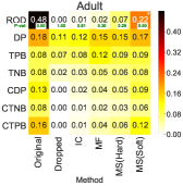
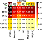
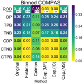
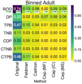
(a) Fairness Comparison of Capuchin for MLP classifier.

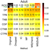
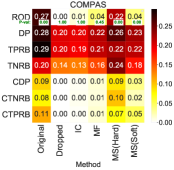
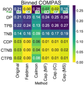
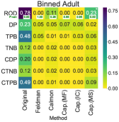
(b) Fairness Comparison of Capuchin for RF classifier.

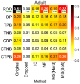
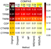
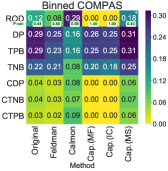
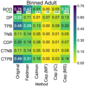
(c) Fairness Comparison of Capuchin for LR classifier.

Figure 7: Bias reduction performance of Capuchin for MLP classifier.

6.3 End-To-End Results

In the following experiments, a fairness constraint was enforced on training data using Capuchin repair algorithms (cf. Sec 4). Specifically, each dataset was split into five training and test datasets. All training data were repaired separately using Matrix Factorization (MF), Independent Coupling (IC) and two versions of the MaxSAT approach: MS(Hard), which feeds all clauses of the lineage of a CI into MaxSAT, and MS(Soft), which only feeds small fraction of the clauses. We tuned MaxSAT to enforce CIs approximately. We then measured the utility and discrimination metrics for each repair method as explained in Sec 6.2. For all datasets, the chosen training variables included the Markov boundary of the outcome variables, which were learned from data using the Grow-Shrink algorithm [31] and permutation [43].

Adult data. Using this dataset, several prior efforts in algorithmic fairness have reported gender discrimination based on a strong statistical dependency between income and gender in favor of males [30, 59, 47]. However, it has been shown that Adult data is inconsistent [43] because its income attribute reports household income for married individuals, and there are more married males in data. Furthermore, data reflects the historical income inequality that can be reinforced by ML algorithms. We used Capuchin to remove the mentioned sources of discrimination from Adult data. Specifically, we categorized the attributes in Adult data as follows: $({\mathbf{S}})$ sensitive attributes: gender (male, female); $({\mathbf{A}})$ admissible attributes: hours per week, occupation, age, education, etc.; $({\mathbf{N}})$ inadmissible attributes: marital status; $(Y)$ binary outcome: high income. As is common in the literature, we assumed that the potential influence of gender on income through some or all of the admissible variables was fair; for example, gender influences education and occupation, which in turn influence income, but, for this experiment, these effects were not considered discriminatory. However, the direct influence of gender on income, as well as its indirect influence on income through marital status, were assumed to be discriminatory. To remove the bias, we enforced the CI $(Y\mbox{$\perp\!\!\!\perp$}{\mathbf{S}},{\mathbf{N}}|{\mathbf{D}})$ on training datasets using the Capuchin repair algorithms. Then, we trained the classifiers on both original and repaired training datasets using the set of variables ${\mathbf{A}}\cup{\mathbf{N}}\cup{\mathbf{S}}$. We also trained the classifiers on original data using only ${\mathbf{A}}$, i.e., we dropped the sensitive and inadmissible variables.

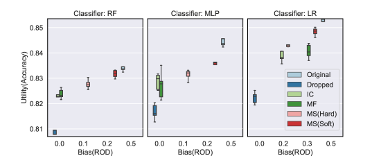
Figure 8: Performance of Capuchin on Adult data.

Fig. 8 compares the utility and bias of Capuchin repair methods on Adult data. As shown, all repair methods successfully reduced the ROD for all classifiers. As shown in Fig. 7, the repaired data also improved associational fairness measures: the Capuchin repair methods had an effect similar to dropping the sensitive and inadmissible variables completely, but they delivered much higher accuracy (because the CI was enforced approximately). The residual bias after repair was expected since: (1) the classifier was only an approximation, and (2) we did not repair the test data. However, as shown in most cases, the residual bias indicated by ROD was not statistically significant. This shows that our methods are robust (by design) to the mismatch between the distribution of repaired data and test data. These repair methods delivered surprisingly good results: when partially repairing data using the MaxSAT approach, i.e, using MS(Soft), almost 50% of the bias was removed while accuracy decreased by only 1%. We also note that the residual bias generally favored the protected group (as opposed to the bias in the original data).

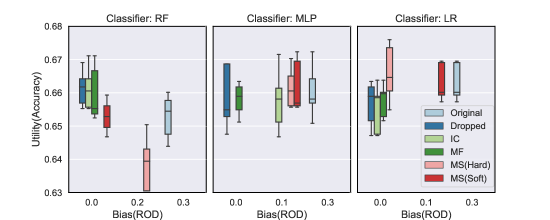
Figure 9: Performance of Capuchin on COMPAS data.

COMPAS. For the second experiment, we used the ProPublica COMPAS dataset [25]. This dataset contains records for all offenders in Broward County, Florida in 2013 and 2014. We categorized the attributes in COMPAS data as follows: $({\mathbf{S}})$ protected attributes: race (African American, Caucasian); $({\mathbf{A}})$ admissible attributes: number of prior convictions, severity of charge degree, age; (Y) binary outcome: a binary indicator of whether the individual is a recidivist. As is common in the literature, we assumed that it was fair to use the admissible attributes to predict recidivism even though they can potentially be influenced by race, and our only goal in this experiment was to address the direct influence of race. We pursued the same steps as explained in the first experiment. Fig. 9 compares the bias and utility of Capuchin repair methods to original data. As shown, all repair methods successfully reduced the ROD. However, we observed that MF and IC performed better than MS on COMPAS data (as opposed to Adult data); see 6.4 for an explanation. We observed that in some cases, repair improved the accuracy of the classifiers on test data by preventing overfitting.

In addition, we used Capuchin to compute the ROD for the COMPAS score and compared it to the same quantity computed for the ground truth. While we obtained a 95% confidence interval of $(0.7,0.9)$ for ROD for ground truth, we obtained a 95% confidence interval of (0.3, 0.5) for ROD for the COMPAS score (high, low). That is, for individuals with the same number of prior convictions and severity of charges, COMPAS overestimated the odds of recidivism by a factor close to 2. The fact that the admissible variables explain the majority of the association between race and recidivism — but not the association between COMPAS scores and recidivism — suggests COMPAS scores are highly racially biased.

6.4 Comparing Capuchin Repair Methods

To compare Capuchin repair methods beyond the utility experiments in Sec 6.3, we compared the number of tuples added and deleted for each method, as well as the bias reduction on training data. Fig 10 reports these measures for the experiments in Sec 6.3. Note that all numbers were normalized between 0 and 1, where ROD=1 shows no discrimination. For Adult data, we tuned the MS approach to repair data only by tuple deletion and compared it to a naive approach that repaired data using lineage expression but without using the MaxSat solver. As shown in Fig 10, the MaxSat approach removed up to 80% fewer tuples than the naive approach.

In general, the MaxSAT approach was the most flexible repair method (since it can be configured for partial repairs). Further, it achieved better classification accuracy, and it balanced tuple insertion and deletion. Further, it could be extended naturally to multiple CIs, though we defer this extension for future work. In terms of the utility of classification, the MS approach performed better on sparse data in which the conditioning groups consisted of several attributes. Figure 11 shows that repairing a very small fraction of inconsistencies (i.e., clauses in the lineage expression of the associated CI) in the experiment conducted on Adult data (Sec 6.3) led to a significant discrimination reduction. This optimization makes the MS approach more appealing in terms of balancing bias and utility. However, for dense data, IC and MD performed better. This difference was because the size of the lineage expression grew very large when the conditioning sets of CIs consisted of only a few attributes.

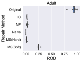
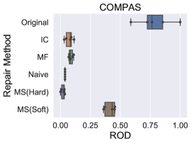
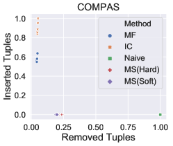
Figure 10: Comparison of different repair methods. All methods successfully enforced fairness constraint, but with different ratio of tuple insertion and deletion. On Adult data MaxSAT outperformed the other methods due to sparsity.

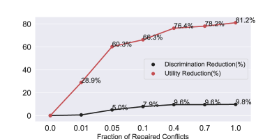
Figure 11: Bias-utility trade off in MaxSAT approach.Repairing only small fraction of conflicts with the fairness constraint in Adult data significantly reduced discrimination.

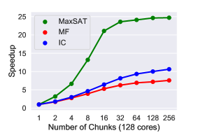
(a)

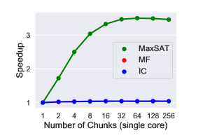
(b)

Figure 12: Speed up achieved (a) by partitioning and parallel processing on 128 cores; (b) by partitioning on a single core.

To evaluate the effect of partitioning and parallelizing on different methods, we replicated the experiment in sec 6.3 and partitioned Adult data into several chunks of approximately equal sizes; we then repaired the chunks in parallel on a cluster of 128 cores. Fig 12 shows the achieved speed up; all approaches were parallelizable. Parallel processing was most appealing for MaxSAT since MaxSAT solvers were much more efficient on smaller input sizes. While partitioning had no effect on MF and IC on a single-core machine, as shown in Fig 12(b), it sped up MaxSAT approach on even a single core. Note that partitioning data into several small chunks does not necessarily speed up the MaxSAT approach, since MaxSAT solver must be called for several small inputs. Hence, performance does not increase linearly by increasing the number of chunks. In general partitioning data into several instance of medium size delivers the best performance.

6.5 Comparing Capuchin to Other Methods

We compared Capuchin  with two reference pre-processing algorithms, Feldman et al. [14] and Calmon et al. [7]. Feldman’s algorithm modifies each attribute so that the marginal distributions based on the subsets of the attribute with a given sensitive value are all equal. Calmon’s algorithm randomly transforms all variables except for the sensitive attribute to reduce the dependence between training labels and the sensitive attribute subject to the following constraints: (1) the joint distribution of the transformed data is close to the original distribution, and (2) individual attributes are not substantially distorted. An example of a distorted attribute in the COMPAS dataset would be changing a felon with no prior conviction to 10 prior convictions. Individual distortion is controlled for using a distortion constraint, which is domain dependent and has to be specified for each dataset. and every single attribute. Note that both approaches are designed to transform training and test data.

We used these algorithm only to repair training datasets and compare their bias and utility to Capuchin. In addition, since the distortion function required in Calmon’s algorithm is completely arbitrary, we replicated the same experiments conducted in [14] using binned Adult data and binned COMPAS data. We note that the analysis in [14] was restricted to only a few attributes, and the data was excessively binned to few categories (to facilitate the definition of distortion function). As a result, the bias and utility obtained in this experiment was mismatched with Sec 6.3. For binned Adult data, the analysis was restricted to age, education and gender. COMPAS data used the same attributes as we used in Sec 6.3. For both datasets, we assumed all attributes were admissible; hence, the direct effect of direct effect of the protected attribute to outcome was removed.

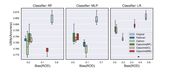
Figure 13: Comparing Capuchin and other methods on Binned Adult data.

Figs. 13 and 14 compares the utility and bias of Capuchin to the reference algorithms. The insights obtained from this experiment follow. For binned Adult data, all methods significantly reduced ROD, even though the goal of Calmon’s and Fledman’s algorithm is essentially to reduce DP. Similarly, Capuchin reduced DP and other associational metrics as a side effect. However, Capuchin outperformed both methods in terms of utility. Because COMPAS data was excessively binned, the ROD in training labels became insignificant for COMPAS, and accuracy dropped by 2%. We observe that both reference algorithms enforced DP at the cost of increasing ROD; however, in some cases the introduced bias was not statistically significant. In terms of utility, all methods of Capuchin (except for MaxSAT) performed better than Feldman’s algorithm, and all Capuchin methods outperformed Calmon’s algorithm quite significantly. This experiment shows that enforcing DP, while unnecessary, can severely affect the accuracy of a classifier and, even more importantly, introduce bias in sub-populations.

This experiment shows that enforcing DP, while unnecessary, can severely affect the accuracy of a classifier and, even more importantly, introduce bias in sub-populations. In this case, while the overall average of recidivism for protected and privileged groups became more balanced using these approaches, the classifier became unfair toward people with the same number of convictions and charge degrees. We note that the observed bias was toward the majority group. Note that Capuchinś MS approach did not perform well on either of these datasets (as opposed to the original data) because of data density. Also note that for COMPAS data, Capuchin delivered better overall utility than the original data because, for Calmon’s dataset (as opposed to the original data), we observed that dropping race indeed increased the accuracy of both RF and MLP classifiers.

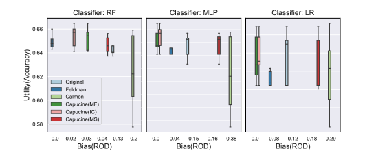
Figure 14: Comparing Capuchin and other methods on Binned COMPAS data.

7 Conclusions and Future Work

We considered a causal approach for fair ML, reducing it to a database repair problem. We showed that conventional fairness metrics, including some causal approaches, end up as variants of statistical parity due to the assumptions they make, and that all associational metrics can over- and under-report discrimination due to statistical anomalies such as Simpson’s Paradox.

Instead, we make explicit the assumptions for admissible variables — variables through which it is permissible for the protected attribute to influence the outcome. We use these assumptions to define a new notion of fairness and to reason about previous definitions. We then prove sufficient properties for fairness and use these results to translate the properties into saturated conditional independences that we can interpret as multivalued dependencies with which to repair the data. We then propose multiple algorithms for implementing these repairs by casting the problem in terms of Matrix Factorization and MaxSAT.

Our experimental results show that our algorithms not only outperform state-of-the-art pre-processing approaches for fairness on our own metrics, but that they are also competitive with existing approaches on conventional metrics. We empirically show that our methods are robust to unseen test data. Our results represent an initial attempt to link the language of causality with database dependencies.

In future work, we aim to study the effect of training databases that are non-representative of the underling population on our results. Currently, our proofs assume that the classifier approximates the true distribution, which is a common assumption in the machine learning literature. However, another important source of discrimination is selection bias or non-representativeness, which we must also correct. Our methods do correct for these forms of bias empirically, but we aim to prove bounds on the fairness metrics based on divergence between training data and test data.

8 Appendix

8.1 Additional Background

New Proof of Impossibility Result in  [9]

Chouldechova [9] proves the following impossibility result: the Equalized Odds and Predictive Parity are impossible to achieve simultaneously when prevalence of the two populations differs, meaning ${\tt\mathrm{Pr}}(Y=1|S=0)\neq{\tt\mathrm{Pr}}(Y=1|S=1)$. The proof follows immediately from her observation that, for each population group $S=i$, the following holds:

$$\frac{{\tt\mathrm{Pr}}(O=1|S=i,Y=0)}{{\tt\mathrm{Pr}}(O=1|S=i,Y=1)}= \frac{{\tt\mathrm{Pr}}(Y=1|S=i)}{{\tt\mathrm{Pr}}(Y=0|S=i)}\frac{{\tt\mathrm{Pr}}(Y=0|O=1,S=i)}{{\tt\mathrm{Pr}}(Y=1|O=1,S=i)}$$

The following provides a simple alternative proof of the impossibility result using conditional independence.

Proposition 8.1

For any probability distribution ${\tt\mathrm{Pr}}$, if $S\mbox{$\perp\!\!\!\perp$}O|Y$ and $S\mbox{$\perp\!\!\!\perp$}Y|O$ then $S\mbox{$\perp\!\!\!\perp$}Y$.

Proof of Proposition 8.1 :

From $S\mbox{$\perp\!\!\!\perp$}O|Y$ and $S\mbox{$\perp\!\!\!\perp$}Y|O$ it follows that ${\tt\mathrm{Pr}}(S|Y)=P(S|O)$ (1), which in turns implies ${\tt\mathrm{Pr}}(Y|S){\tt\mathrm{Pr}}(O)={\tt\mathrm{Pr}}(O|S){\tt\mathrm{Pr}}(Y)$ (apply Bayes rule to the both sides of (1)). By summarization over $O$ we get ${\tt\mathrm{Pr}}(Y|S)={\tt\mathrm{Pr}}(Y)$, which completes the proof. $\square$

Implication Problem for CIs

The implication problem for CI is the problem of deciding whether a CI $\varphi$ is logically follows from a set of CIs $\Sigma$, meaning that in every distribution in which $\Sigma$ holds, $\varphi$ also holds. The following set of sound but incomplete axioms, known as Graphoid, are given in [38] for this implication problem.

Suppose $\mathbf{A}$ consists of a set of protected attributes ${\mathbf{P}}$ such as race and gender; a set of attributes ${\mathbf{X}}$ that might be used for decision making, e.g., credit score; a binary outcome attribute $Y$, e.g., good or bad credit score. Assume a classifier is trained on $S\subseteq{\mathbf{P}}\cup{\mathbf{X}}$ to predict $Y$. Suppose $O$ consists of the classifier decisions. Throughout this paper we assume the classifier provides a good appropriation of the conditional distribution of $Y$, i.e., ${\tt\mathrm{Pr}}(Y|S)\approx{\tt\mathrm{Pr}}(O|S)$.

• (Symmetry)

  $$({\mathbf{X}}\mbox{$\perp\!\!\!\perp$}{\mathbf{Y}}|{\mathbf{Z}})\rightarrow({\mathbf{Y}}\mbox{$\perp\!\!\!\perp$}{\mathbf{X}}|{\mathbf{Z}})$$ (12)

• (Decomposition)

  $$({\mathbf{X}}\mbox{$\perp\!\!\!\perp$}{\mathbf{W}}{\mathbf{Y}}|{\mathbf{Z}})\rightarrow({\mathbf{X}}\mbox{$\perp\!\!\!\perp$}{\mathbf{W}}|{\mathbf{Z}})$$ (13)

• (Weak Union)

  $$({\mathbf{X}}\mbox{$\perp\!\!\!\perp$}{\mathbf{W}}{\mathbf{Y}}|{\mathbf{Z}})\rightarrow({\mathbf{X}}\mbox{$\perp\!\!\!\perp$}{\mathbf{Y}}|{\mathbf{Z}}{\mathbf{W}})$$ (14)

• (Contraction)

  $$({\mathbf{X}}\mbox{$\perp\!\!\!\perp$}{\mathbf{Y}}|{\mathbf{W}}{\mathbf{Z}})\land({\mathbf{X}}\mbox{$\perp\!\!\!\perp$}{\mathbf{W}}|{\mathbf{Z}})\rightarrow({\mathbf{X}}\mbox{$\perp\!\!\!\perp$}{\mathbf{Y}}{\mathbf{W}}|{\mathbf{Z}})$$ (15)

For strictly positive distribution in addition to the above the following axiom also holds:

• (Intersection)

  $$({\mathbf{X}}\mbox{$\perp\!\!\!\perp$}{\mathbf{Y}}|{\mathbf{W}}{\mathbf{Z}})\land({\mathbf{X}}\mbox{$\perp\!\!\!\perp$}{\mathbf{W}}|{\mathbf{Y}}{\mathbf{Z}})\rightarrow({\mathbf{X}}\mbox{$\perp\!\!\!\perp$}{\mathbf{Y}}{\mathbf{W}}|{\mathbf{Z}})$$ (16)

Causal Models

A probabilistic causal model (PCM) is a tuple ${{{\mathbf{M}}}}=\langle{\mathbf{U}},{\mathbf{V}},{\mathbf{F}},{\tt\mathrm{Pr}}_{{\mathbf{U}}}\rangle$, where ${\mathbf{U}}$ is a set of background or exogenous variables that cannot be observed but which can influence the rest of the model; ${\mathbf{V}}$ is a set of observable or endogenous variables; ${\mathbf{F}}=(F_{X})_{X\in{\mathbf{V}}}$ is a set of structural functions $F_{X}\mathrel{\mathop{\ordinarycolon}}Dom({\mathbf{Pa}}_{{\mathbf{U}}}(X))\times Dom({\mathbf{Pa}}_{{\mathbf{V}}}(X))\rightarrow Dom(X)$, where ${\mathbf{Pa}}_{{\mathbf{U}}}(X)\subseteq{\mathbf{U}}$ and ${\mathbf{Pa}}_{{\mathbf{V}}}(X)\subseteq{\mathbf{V}}-\mathinner{\left\{X\right\}}$ are called the exogenous parents and endogenous parents of $X$ respectively; and ${\tt\mathrm{Pr}}_{{\mathbf{U}}}$ is a joint probability distribution on the exogenous variables ${\mathbf{U}}$. Intuitively, the exogenous variables ${\mathbf{U}}$ are not known, but we know their probability distribution, while the endogenous variables are completely determined by their parents (exogenous and/or endogenous).

Causal DAG

To each PCM ${{{\mathbf{M}}}}$ we associate a causal graph $G$ with nodes consisting of the endogenous variables ${\mathbf{V}}$, and edges consisting of all pairs $(Z,X)$ such that $Z\in{\mathbf{Pa}}_{{\mathbf{V}}}(X)$; we write $Z\rightarrow X$ for an edge. $G$ is always assumed to be acyclic, and called Causal DAG. One can show that the probability distribution on the exogenous variables uniquely determined a distribution ${\tt\mathrm{Pr}}_{{\mathbf{V}}}$ on the endogenous variables and, under the causal sufficiency assumption, ${\tt\mathrm{Pr}}_{{\mathbf{V}}}$ forms a Bayesian network, whose graph is exactly $G$:

$${\tt\mathrm{Pr}}({\mathbf{V}})= \prod_{X\in{\mathbf{V}}}{\tt\mathrm{Pr}}(X|{\mathbf{Pa}}(X))$$ (17)

Thus justifies omitting the exogenous variables from the causal DAG, and capturing their effect through the probability distribution Eq.(17). We will only refer to endogenous variables, and drop the subscript ${\mathbf{V}}$ from ${\mathbf{Pa}}_{{\mathbf{V}}}$ and ${\tt\mathrm{Pr}}_{{\mathbf{V}}}$. A path in $G$ means an undirected path, i.e. we may traverse edges either forwards or backwards; a directed path is one where we traverse edges only forwards.

d-Separation

We review the notion of d-separation, which is the graph-theoretic characterization of conditional independence. A path ${\mathbf{P}}$ from $X$ to $Y$ is a sequence of nodes $X=V_{1},\ldots,V_{\ell}=Y$ such that $V_{i}\rightarrow V_{i+1}$ or $V_{i}\leftarrow V_{i+1}$ forall $i$. ${\mathbf{P}}$ is directed if $V_{i}\rightarrow V_{i+1}$ forall $i$, and in that case we write $X\stackrel{{\scriptstyle*}}{{\rightarrow}}Y$, and say that $X$ is an ancestor, or a cause of $Y$, and $Y$ is a descendant or an effect of $X$. If the path contains a subsequence $V_{k-1}\rightarrow V_{k}\leftarrow V_{k+1}$ then $V_{k}$ is called a collider. A path with a collider is closed; otherwise it is open; an open path has the form $X\stackrel{{\scriptstyle*}}{{\leftarrow}}\stackrel{{\scriptstyle*}}{{\rightarrow}}Y$, i.e. $X$ causes $Y$ or $Y$ causes $X$ or they have a common cause. Given two sets of nodes ${\mathbf{X}},{\mathbf{Y}}$ we say that a set ${\mathbf{Z}}$ d-separates ${\mathbf{X}}$ and ${\mathbf{Y}}$, denoted by $({\mathbf{X}}\mbox{$\perp\!\!\!\perp$}{\mathbf{Y}}|_{d}\ {\mathbf{Z}})$, if for any all paths $P$ from ${\mathbf{X}}$ to ${\mathbf{Y}}$ one of the followings hold: (1) ${\mathbf{P}}$ is closed at a collider node $V$ such that neither $V$ nor any of its descendants are in ${\mathbf{Z}}$; (2) ${\mathbf{P}}$ contains a non-collider node $V^{\prime}$ such that $V^{\prime}\in{\mathbf{P}}$. We say that a set ${\mathbf{Z}}$. d-Separation is a sufficient condition for conditional independence, see Prop. 2.1

General Identification Criterion

In the presence of unrecorded variables in the causal DAG, the effect of interventions can not be identified using Eq. 2. A set of sound and complete axioms known as $do$-calculus can be used to decide whether the effect of intervention can be identified from the observed distribution [35]. If the effect is identifiable then by repeatedly applying the rules of do-calculus, one can obtain an statement equivalent to Eq. 2, but free from unobserved variables. Since identification is not the focus of this paper, we assume all variables are observed hence Theorem 2.2 is sufficient for identification.

Markov Blanket

We briefly review the notion of Markov blanket, which used in Sec 3.2.

Definition 8.2

[36] Fix a joint probability distribution ${\tt\mathrm{Pr}}({\mathbf{v}})$ and a variable $X\in{\mathbf{V}}$. A set of variables ${\mathbf{B}}(X)\subseteq{\mathbf{V}}-\mathinner{\left\{X\right\}}$ is called a Markov Blanket of $X$ if $(X\mbox{$\perp\!\!\!\perp$}{\mathbf{V}}-{\mathbf{B}}(X)-\mathinner{\left\{X\right\}}|{\mathbf{B}}(X))$; it is called a Markov Boundary if it is minimal w.r.t. set inclusion, denoted ${\bf MB}(X)$.

In the admission process in Fig 2.3 ${\bf MB}(X)=\{D,H\}$, simply because $O\mbox{$\perp\!\!\!\perp$}G|H,D$ (since $\mathinner{\left\{H,D\right\}}$ d-separate $O$ and $G$). It is known that if ${\tt\mathrm{Pr}}$ is a strictly positive distribution (i.e., forall ${\mathbf{v}}\in Dom({\mathbf{V}}),P({\mathbf{v}})>0$), then ${\bf MB}(V)$ is unique for all $V\in{\mathbf{V}}$ and can be learned from data in polynomial time [31]. Strictly positive distributions do not allows for logical functional dependencies between their variables. The requirement can be satisfied in data by removing logical dependencies [43]. Note that under the faithfulness assumption, the Markov boundary of a node $X$ in the causal graph consists of the parents of $X$, the children of $X$, and the parents of the children of $X$ [34].

Note that if ${\mathbf{X}}$ is the set of all inputs of the algorithm included in data, then ${\bf MB}(O)={\mathbf{X}}$, i.e., parents of $X$ form a boundary for $O$. This is because $(O\mbox{$\perp\!\!\!\perp$}{\mathbf{V}}-{\mathbf{X}}|{\mathbf{X}})$ is implied from the functional dependency (FD) ${\mathbf{X}}\rightarrow O$, which can be discovered from data by a linear search through the attributes. Hence, ROD essentially requires that conditioned on admissible inputs of ${\mathbf{X}}\cap{\mathbf{A}}$, the outcome of algorithm becomes independent of the protected attribute, meaning the algorithm treats similarly individuals that are similar on ${\mathbf{X}}\cap{\mathbf{A}}$ characteristics but different in $S$. Any imbalance indicated by ROD is worrisome and requires scrutiny. Also note that in general Markov boundary can be learned from data by the linear number of iterations through the variables [31].

Proposition 8.3

Fix a strictly positive probability distribution ${\tt\mathrm{Pr}}_{{\mathbf{V}}}$. It holds that for any variable $V\in{\mathbf{V}}$, the unique Markov boundary of $V$, ${\bf MB}(V)$ is unique.

Proof of Proposition 8.3 :

The uniqueness of the Markov Boundary is implied from the intersection axiom (cf. Eq 16) as follows: Without loss of generality suppose ${\mathbf{V}}=V{\mathbf{X}}{\mathbf{W}}{\mathbf{Z}}{\mathbf{Y}}$, where ${\mathbf{X}}$ and ${\mathbf{Y}}$ are disjoint. We show that if two sets ${\mathbf{X}}{\mathbf{Z}}$ and ${\mathbf{Y}}{\mathbf{Z}}$ form a Markov boundary for $V$ then their intersection, i.e, $Z$ is a Markov blanket for $V$. This contradicts the subset minimality of a Markov boundary. We show this in the following steps using Graphoid axioms.

$$V \mbox{$\perp\!\!\!\perp$}{\mathbf{W}},{\mathbf{Y}}|{\mathbf{X}}{\mathbf{Z}}$$ (18)

$$V \mbox{$\perp\!\!\!\perp$}{\mathbf{W}},{\mathbf{X}}|{\mathbf{Y}}{\mathbf{Z}}$$ (19)

$$V \mbox{$\perp\!\!\!\perp$}{\mathbf{Y}},{\mathbf{X}}|{\mathbf{Z}}\hskip 14.22636pt\text{By (\ref{mb1}) , (\ref{mb2}) Dec. and Inter. axioms}$$ (20)

$$V \mbox{$\perp\!\!\!\perp$}{\mathbf{W}}|{\mathbf{X}}{\mathbf{Z}}{\mathbf{Y}}\hskip 8.5359pt\text{By (\ref{mb1}) and Weak Union}$$ (21)

$$V \mbox{$\perp\!\!\!\perp$}{\mathbf{W}}{\mathbf{X}}{\mathbf{Y}}|{\mathbf{Z}}\hskip 8.5359pt\text{By (\ref{inter}) , (\ref{wu}) and Contraction}$$

Therefore, Markov Boundary of $V$ is unique. $\square$

Counterfactual Fairness

Given a set of features ${\mathbf{X}}$, a protected attribute $S$, an outcome variable $Y$, and a set of unobserved background variables ${\mathbf{U}}$, Kusner et al. [23] defined a predictor $\tilde{Y}$ to be counterfactually fair if for any ${\mathbf{x}}\in Dom({\mathbf{X}})$:

$$P(\tilde{Y}_{S\leftarrow 0}({\mathbf{U}})=1|{\mathbf{X}}={\mathbf{x}},S=1)=P(\tilde{Y}_{S\leftarrow 1}({\mathbf{U}})=1|{\mathbf{X}}={\mathbf{x}};S=1)$$ (22)

where, $\tilde{Y}_{S\leftarrow s}({\mathbf{U}})$ means intervening on the protected attribute in an unspecified configuration of the exogenous factors. The definition meant to capture the requirement that the protected attribute $S$ should not be a cause of $\tilde{Y}$ at individual level. However, it fails on the simple example in Ex 3.2. This is because, $P({O}_{G\leftarrow g}(U_{O})=1)=P(U_{O}=1)P({Y}_{G\leftarrow g}(U_{O})=1|U_{O}=1)=\frac{1}{2}$ for $g=\mathinner{\left\{0,1\right\}}$. We note that the stricter version of counterfactual fairness in [24] also fails to capture the individual-level unfairness in this example. We report that this observation has been confirmed by the authors of [24]. We defer the full comparison for future work.

Proof of Lemma 5.1 :

Because the classifier is a deterministic function trained on ${\tt\mathrm{Pr}}_{B^{\prime}}$, it follows that ${\tt\mathrm{Pr}}_{T}(o,s,i,a)={\tt\mathrm{Pr}}_{B^{\prime}}(o,s,i,a)={\tt\mathrm{Pr}}_{B^{\prime}}(o|a){\tt\mathrm{Pr}}_{B^{\prime}}(i,s,a)$. Hence it is sufficient to show that $D_{KL}({\tt\mathrm{Pr}}_{T}(o|s,i,a)\;||\;{\tt\mathrm{Pr}}_{T}(o|a))=0$ or ${\tt\mathrm{Pr}}_{T}(o|s,i,a)={\tt\mathrm{Pr}}_{T}(o|a)$. We show this in the following steps:

$${\tt\mathrm{Pr}}_{T}(o|s,i,a)= \frac{{\tt\mathrm{Pr}}_{T}(o,s,i,a)}{{\tt\mathrm{Pr}}_{T}(s,i,a)}$$ (23)

$$= \frac{{\tt\mathrm{Pr}}_{B^{\prime}}(o,s,i,a)}{{\tt\mathrm{Pr}}_{T}(s,i,a)}$$ (24)

$$= \frac{{\tt\mathrm{Pr}}_{B^{\prime}}(o|a){\tt\mathrm{Pr}}_{B^{\prime}}(s,i,a)}{{\tt\mathrm{Pr}}_{T}(s,i,a)}$$ (25)

$${\tt\mathrm{Pr}}_{T}(o|a)= \frac{{\tt\mathrm{Pr}}_{T}(o,a)}{{\tt\mathrm{Pr}}_{T}(a)}$$ (26)

$$= \frac{\sum_{s,i}{\tt\mathrm{Pr}}_{B^{\prime}}(o,i,s,a)}{{\tt\mathrm{Pr}}_{T}(a)}$$ (27)

$$= \frac{\sum_{s,i}{\tt\mathrm{Pr}}_{B^{\prime}}(o|a){\tt\mathrm{Pr}}_{B^{\prime}}(s,i,a)}{{\tt\mathrm{Pr}}_{T}(a)}$$ (28)

$$= \frac{{\tt\mathrm{Pr}}_{B^{\prime}}(o|a){\tt\mathrm{Pr}}_{B^{\prime}}(a)}{{\tt\mathrm{Pr}}_{T}(a)}$$ (29)

Hence,

$$D_{KL}(pr_{T}(o|s,i,a)\;||\;pr_{T}(o|a))$$ (30)

$$=-\sum{\tt\mathrm{Pr}}_{T}(o|i,s,a)\log\frac{{\tt\mathrm{Pr}}_{T}(o|a)}{{\tt\mathrm{Pr}}_{T}(o|s,i,a)}$$ (31)

$$=-\sum{\tt\mathrm{Pr}}_{T}(o|i,s,a)\log\frac{\frac{{\tt\mathrm{Pr}}_{B^{\prime}}(o|a){\tt\mathrm{Pr}}_{B^{\prime}}(a)}{pr_{T}(a)}}{\frac{{\tt\mathrm{Pr}}_{B^{\prime}}(o|a){\tt\mathrm{Pr}}_{B^{\prime}}(i,s,a)}{{\tt\mathrm{Pr}}_{T}(s,i,a)}}$$ (32)

$$=-\sum{\tt\mathrm{Pr}}_{T}(o|i,s,a)\log\frac{{\tt\mathrm{Pr}}_{B^{\prime}}(s,i|a)}{{\tt\mathrm{Pr}}_{T}(s,i|a)}$$ (33)

Thus, $D_{KL}({\tt\mathrm{Pr}}_{T}(o|s,i,a)\;||\;{\tt\mathrm{Pr}}_{T}(o|a))=0$ if ${\tt\mathrm{Pr}}_{T}(s,i|a){\tt\mathrm{Pr}}_{B^{\prime}}(s,i|a)$, which implies ${\tt\mathrm{Pr}}_{T}(o|s,i,a)={\tt\mathrm{Pr}}_{T}(o|a)$ or equivalently that $(Y\mbox{$\perp\!\!\!\perp$}S,{\mathbf{I}}|_{\Pr_{T}}{\mathbf{A}})$. This completes the proof.

$\square$

8.2 Proofs and Supplementary Propositions and graphs

Proof of Theorem 2.2 :

Recall that a causal $G$ admits the following factorization of the observed distribution:

$$\Pr({\mathbf{v}})=\prod_{V\in{\mathbf{V}}}\Pr(v|{\mathbf{pa}}(V))$$ (34)

Now, each atomic intervention $do(X=x)$ modifies the causal DAG $G$ by removing parents of $X$ from $G$. Therefore, the probability distribution $P({\mathbf{v}}|do({\mathbf{X}}={\mathbf{x}}))$ can be obtained from the observed distribution $P({\mathbf{v}})$ by removing all factors $\Pr(x|{\mathbf{pa}}(X))$, for $X\in{\mathbf{X}}$, from $P({\mathbf{v}})$, i.e.,

$$\Pr({\mathbf{v}}|do({\mathbf{X}}={\mathbf{x}})) = \frac{\Pr({\mathbf{v}})}{\prod_{i=0}^{m}{\tt\mathrm{Pr}}(x_{i}|{\mathbf{pa}}(X_{i}))}$$ (35)

The following holds according to the chain rule of probability:

$$\Pr({\mathbf{v}}) = \prod_{i=0}^{m}\bigg{(}\Pr\big{(}{\mathbf{pa}}(X_{i})|\bigcup_{j=0}^{i-1}{\mathbf{pa}}(X_{j}),\bigcup_{j=0}^{i-1}x_{j}\big{)}\bigg{)}\bigg{(}\Pr(x_{i}|\bigcup_{j=0}^{i}{\mathbf{pa}}(X_{j}),\bigcup_{j=0}^{i-1}x_{j})\bigg{)}$$

$${\tt\mathrm{Pr}}({\mathbf{w}}|{\mathbf{x}},{\mathbf{z}})$$ (36)

where, ${\mathbf{Z}}=\bigcup_{X\in{\mathbf{X}}}{\mathbf{Pa}}(X)$, ${\mathbf{W}}={\mathbf{V}}-({\mathbf{X}}\cup{\mathbf{Z}})$ and $j\geq 0$. It holds that in a causal DAG $G$, any node $X\in{\mathbf{V}}$ is independent of its non-descendant condition on it parents ${\mathbf{Pa}}(X)$ (known as Markov property [36]). This is simply because ${\mathbf{Pa}}(X)$ d-separates $X$ from its non-descendants. Therefore, the following is implied from the assumption that $X_{i}$ is an non-descendant of $X_{i+1}$:

$$\Pr(x_{i}|\bigcup_{j=0}^{i}{\mathbf{pa}}(X_{j}),\bigcup_{j=0}^{i-1}x_{j})=\Pr(x_{i}|{\mathbf{pa}}(X_{i}))\ \text{for}\ i=0,m$$ (37)

Hence,

$$\Pr({\mathbf{v}}) = \bigg{(}\prod_{i=0}^{m}\Pr\big{(}{\mathbf{pa}}(X_{i})|\bigcup_{j=0}^{i-1}{\mathbf{pa}}(X_{j}),\bigcup_{j=0}^{i-1}x_{j}\big{)}\bigg{)}\bigg{(}\prod_{i=0}^{m}\Pr(x_{i}|{\mathbf{P}}a(X_{i}))\bigg{)}$$

$${\tt\mathrm{Pr}}({\mathbf{w}}|{\mathbf{x}},{\mathbf{z}})$$ (38)

The following implied from Eq. 38 and 35.

$$\Pr({\mathbf{v}}|do({\mathbf{X}}={\mathbf{x}}))= \frac{\Pr({\mathbf{v}})}{\prod_{i=0}^{m}{\tt\mathrm{Pr}}(x_{i}|{\mathbf{pa}}(X_{i}))}$$

$$=\bigg{(}\prod_{i=0}^{m}\Pr\big{(}{\mathbf{pa}}(X_{i})|\bigcup_{j=0}^{i-1}{\mathbf{pa}}(X_{j}),\bigcup_{j=0}^{i-1}x_{j}\big{)}\bigg{)}{\tt\mathrm{Pr}}({\mathbf{w}}|{\mathbf{x}},{\mathbf{z}})$$ (39)

Now, by summation over all variables except for $Y$ and ${\mathbf{X}}$ in Eq. 39 we obtain the following, which proves the theorem.

$$P(y|do({\mathbf{X}}={\mathbf{x}}))=\sum_{{\mathbf{z}}\in{\mathbf{Z}}}\Pr(y|{\mathbf{x}},{\mathbf{z}})\bigg{(}\prod_{i=0}^{m}\Pr\big{(}{\mathbf{pa}}(X_{i})|\bigcup_{j=0}^{i-1}{\mathbf{pa}}(X_{j}),\bigcup_{j=0}^{i-1}x_{j}\big{)}\bigg{)}$$ (40)

$\square$

Proof of Proposition 3.5 :

In one direction, we note that, for any choice of ${\mathbf{K}}$, the causal graph corresponding to an intervention $do({\mathbf{K}}={\mathbf{k}})$ disconnects $S$ and $O$, and therefore intervening on $S$ does not affect $O$. In the other direction, let ${\mathbf{P}}$ be a path from $S$ to $O$ s.t. ${\mathbf{P}}\cap{\mathbf{A}}=\emptyset$, and let ${\mathbf{K}}$ be the set of all variables not in ${\mathbf{P}}$; in particular, ${\mathbf{A}}\subseteq{\mathbf{K}}$. The causal graph corresponding to an intervention on ${\mathbf{K}}$ consists of a single path $S\rightarrow^{*}O$ because all other edges are removed by the intervention. Since $S$ has no parents, intervening on $S$ is the same as conditioning on $S$, and, since ${\tt\mathrm{Pr}}$ is faithful, we have ${\tt\mathrm{Pr}}(O=o|S=0)\neq{\tt\mathrm{Pr}}(O=0|S=1)$ for some outcome $O=o$, contradicting the assumption of ${\mathbf{K}}$-fairness. $\square$

Proof of Theorem 3.7 :

We show that an algorithm $\mathcal{A}$ is ${\mathbf{A}}$-fair if ${\bf MB}(O)\subseteq{\mathbf{A}}$. From Theorem 2.2, we obtain:

$${\tt\mathrm{Pr}}(O=o|do(S=i),do({\mathbf{A}}={\mathbf{a}}))=\sum_{{\mathbf{z}}\in Dom({\mathbf{Z}})}{\tt\mathrm{Pr}}(y|S=i,{\mathbf{A}}={\mathbf{a}},{\mathbf{z}})$$

$$\bigg{(}\prod_{i=0}^{m}{\tt\mathrm{Pr}}\big{(}{\mathbf{pa}}(X_{i})\bigg{|}\bigcup_{j=0}^{i-1}{\mathbf{pa}}(X_{j}),\bigcup_{j=0}^{i-1}x_{j}\big{)}\bigg{)}$$ (41)

where, ${\mathbf{Z}}=\bigcup_{A\in{\mathbf{A}}}{\mathbf{Pa}}(A)$. Without loss of generality assume ${\mathbf{Z}}\cap{\mathbf{A}}^{\prime}=\emptyset$. Let ${\mathbf{A}}={\bf MB}(O)\cup{\mathbf{A}}^{\prime}$ and ${\mathbf{V}}^{\prime}={\mathbf{V}}-\{{\mathbf{A}}^{\prime}\cup{\mathbf{Z}}\cup\mathinner{\left\{S\right\}}\}$. From the definition of Markov boundary we have $(O\mbox{$\perp\!\!\!\perp$}{\mathbf{V}}^{\prime},{\mathbf{A}}^{\prime},S,{\mathbf{Z}}|{\bf MB}(O))$. It follows from Decomposition and Weak Union axioms in Graphoid that $(O\mbox{$\perp\!\!\!\perp$}S,{\mathbf{Z}}|{\bf MB}(O),{\mathbf{A}}^{\prime})$, hence $(O\mbox{$\perp\!\!\!\perp$}S,{\mathbf{Z}}|{\mathbf{A}})$. We obtain the following for $i=\{0,1\}$:

$${\tt\mathrm{Pr}}(O=o|do(S=i),do({\mathbf{A}}={\mathbf{a}})) = {\tt\mathrm{Pr}}(y|A={\mathbf{a}})$$ (42)

$$\sum_{{\mathbf{z}}\in Dom({\mathbf{Z}})}\bigg{(}\prod_{i=0}^{m}{\tt\mathrm{Pr}}\big{(}{\mathbf{pa}}(X_{i})\bigg{|}\bigcup_{j=0}^{i-1}{\mathbf{pa}}(X_{j}),\bigcup_{j=0}^{i-1}x_{j}\big{)}\bigg{)}$$

$$= {\tt\mathrm{Pr}}(y|A={\mathbf{a}})\noindent$$

Note that (42) obtained by the fact that each product inside the summation becomes 1 (simply because $\sum_{X}{\tt\mathrm{Pr}}(X|Y)=1$) This proves the ${\mathbf{A}}$-fairness of $\mathcal{A}$. ${\mathbf{K}}$-fairness for each ${\mathbf{K}}\supseteq{\mathbf{A}}$ can be proved in a similar way. $\square$

Proof of Corollary 3.8 :

Without loss of generality, suppose ${\mathbf{V}}=Y{\mathbf{D}}{\mathbf{Z}}{\mathbf{W}}{\mathbf{U}}$ with ${\mathbf{X}}={\mathbf{A}}\cup{\mathbf{Z}}$ and ${\mathbf{A}}={\mathbf{W}}\cup{\mathbf{Z}}$. Since the classifier is trained on ${\mathbf{X}}$, there is a functional dependency ${\mathbf{X}}\rightarrow O$, which implies $(O\mbox{$\perp\!\!\!\perp$}{\mathbf{Y}},{\mathbf{W}},{\mathbf{U}}|{\mathbf{A}},{\mathbf{Z}})$(1), i.e., ${\mathbf{X}}$ forms a Markov blanket for $O$. It is also implied from the assumptions ${\tt\mathrm{Pr}}(Y=1|{\mathbf{X}}={\mathbf{x}})\approx{\tt\mathrm{Pr}}(O=1|{\mathbf{X}}={\mathbf{x}})$ and $(Y\mbox{$\perp\!\!\!\perp$}{\mathbf{X}}-{\mathbf{A}}|{\mathbf{A}}\cap X)$ that $(O\mbox{$\perp\!\!\!\perp$}{\mathbf{A}}|{\mathbf{Z}})$ approximately holds (2). By applying the Contraction axiom in Graphoid to (1) and (2), we obtain $(O\mbox{$\perp\!\!\!\perp$}Y{\mathbf{A}},{\mathbf{W}},{\mathbf{U}}|{\mathbf{Z}})$ i.e., ${\bf MB}(O)\subseteq{\mathbf{A}}$. Therefore, $\mathcal{A}$ is justifiably fair according to Theorem 3.7. This completes the proof of part (a). Part (b) is implied from part(1), definition of Markov boundary and Decomposition axiom in Graphoid. $\square$

Proposition 8.4

Given a fairness application $(\mathcal{A},S,{\mathbf{A}},{\mathbf{I}})$, suppose the probability distribution of $\mathcal{A}$ is faithful to the causal DAG. Then, the application is justifiably fair iff $\delta(S;O|\linebreak{\mathbf{{\bf MB}}}(O)\cap{\mathbf{A}})=1$.

Proof of Proposition 8.4 :

It is easy to see $\delta(S;O|{\mathbf{{\bf MB}}}(O)$ $\cap{\mathbf{A}})=1$ iff $S\mbox{$\perp\!\!\!\perp$}O|{\mathbf{{\bf MB}}}(O)\cap{\mathbf{A}}$. Under the faithfulness assumption, we obtain ${\bf MB}(O)\cap{\mathbf{A}}$ and d-separates $S$ and $O$. Hence, all directed paths from $S$ to $O$ go thorough ${\mathbf{{\bf MB}}}(O)\cap{\mathbf{A}}$. Therefore, the algorithm is justifiably fair according to Theorem 3.5. The converse is immediate from the natural assumption that $O$ does not have any descendants in the causal DAG; hence, its Markov boundary consists of the algorithm’s inputs. $\square$

Proof of Proposition 4.6 :

The proposition follows from three facts, all easily verified. (1) $D\subseteq D^{*}$, (2) $D^{*}$ satisfies the MVD ${\mathbf{Z}}\twoheadrightarrow{\mathbf{X}}$, and (3) If two databases $D_{1},D_{2}$ satisfy the MVD then so does $D_{1}\cap D_{2}$. Indeed, the three facts imply that, for any repair $D^{\prime}$, the database $D^{*}\cap D^{\prime}$ is also a repair and $|\Delta(D,D^{*}\cap D^{\prime})|\leq\Delta(D,D^{\prime})|$, hence, if $D^{\prime}$ is a minimal repair, then $D^{\prime}\subseteq D^{*}$. $\square$

References

- [1] Serge Abiteboul, Richard Hull, and Victor Vianu. Foundations of Databases. Addison-Wesley, 1995.
- [2] Chen Avin, Ilya Shpitser, and Judea Pearl. Identifiability of path-specific effects. 2005.
- [3] Leopoldo E. Bertossi. Database Repairing and Consistent Query Answering. Synthesis Lectures on Data Management. Morgan & Claypool Publishers, 2011.
- [4] Matthew T Bodie, Miriam A Cherry, Marcia L McCormick, and Jintong Tang. The law and policy of people analytics. U. Colo. L. Rev., 88:961, 2017.
- [5] Toon Calders, Faisal Kamiran, and Mykola Pechenizkiy. Building classifiers with independency constraints. In Data mining workshops, 2009. ICDMW’09. IEEE international conference on, pages 13–18. IEEE, 2009.
- [6] Toon Calders and Sicco Verwer. Three naive bayes approaches for discrimination-free classification. Data Mining and Knowledge Discovery, 21(2):277–292, 2010.
- [7] Flavio Calmon, Dennis Wei, Bhanukiran Vinzamuri, Karthikeyan Natesan Ramamurthy, and Kush R Varshney. Optimized pre-processing for discrimination prevention. In I. Guyon, U. V. Luxburg, S. Bengio, H. Wallach, R. Fergus, S. Vishwanathan, and R. Garnett, editors, Advances in Neural Information Processing Systems 30, pages 3992–4001. Curran Associates, Inc., 2017.
- [8] Bei-Hung Chang and David C Hoaglin. Meta-analysis of odds ratios: Current good practices. Medical care, 55(4):328, 2017.
- [9] Alexandra Chouldechova. Fair prediction with disparate impact: A study of bias in recidivism prediction instruments. Big data, 5(2):153–163, 2017.
- [10] Sam Corbett-Davies, Emma Pierson, Avi Feller, Sharad Goel, and Aziz Huq. Algorithmic decision making and the cost of fairness. In Proceedings of the 23rd ACM SIGKDD International Conference on Knowledge Discovery and Data Mining, pages 797–806. ACM, 2017.
- [11] Rachel Courtland. Bias detectives: the researchers striving to make algorithms fair. Nature, 558, 2018.
- [12] Jeffrey Dastin. Rpt-insight-amazon scraps secret ai recruiting tool that showed bias against women. Reuters, 2018. https://www.reuters.com/article/amazoncom-jobs-automation/rpt-insight-amazon-scraps-secret-ai-recruiting-tool-that-showed-bias-against-women-idUSL2N1WP1RO.
- [13] Cynthia Dwork, Moritz Hardt, Toniann Pitassi, Omer Reingold, and Richard Zemel. Fairness through awareness. In Proceedings of the 3rd innovations in theoretical computer science conference, pages 214–226. ACM, 2012.
- [14] Michael Feldman, Sorelle A Friedler, John Moeller, Carlos Scheidegger, and Suresh Venkatasubramanian. Certifying and removing disparate impact. In Proceedings of the 21th ACM SIGKDD International Conference on Knowledge Discovery and Data Mining, pages 259–268. ACM, 2015.
- [15] Cédric Févotte and Jérôme Idier. Algorithms for nonnegative matrix factorization with the -divergence. Neural computation, 23(9):2421–2456, 2011.
- [16] Sainyam Galhotra, Yuriy Brun, and Alexandra Meliou. Fairness testing: testing software for discrimination. In Proceedings of the 2017 11th Joint Meeting on Foundations of Software Engineering, pages 498–510. ACM, 2017.
- [17] Moritz Hardt, Eric Price, Nati Srebro, et al. Equality of opportunity in supervised learning. In Advances in neural information processing systems, pages 3315–3323, 2016.
- [18] Joachim Hartung. A note on combining dependent tests of significance. Biometrical Journal: Journal of Mathematical Methods in Biosciences, 41(7):849–855, 1999.
- [19] David Ingold and Spencer Soper. Amazon doesn’t consider the race of its customers. should it? Bloomberg, 2016. www.bloomberg.com/graphics/2016-amazon-same-day/.
- [20] Faisal Kamiran and Toon Calders. Classifying without discriminating. In Computer, Control and Communication, 2009. IC4 2009. 2nd International Conference on, pages 1–6. IEEE, 2009.
- [21] Toshihiro Kamishima, Shotaro Akaho, Hideki Asoh, and Jun Sakuma. Fairness-aware classifier with prejudice remover regularizer. In Joint European Conference on Machine Learning and Knowledge Discovery in Databases, pages 35–50. Springer, 2012.
- [22] Niki Kilbertus, Mateo Rojas Carulla, Giambattista Parascandolo, Moritz Hardt, Dominik Janzing, and Bernhard Schölkopf. Avoiding discrimination through causal reasoning. In Advances in Neural Information Processing Systems, pages 656–666, 2017.
- [23] Matt J Kusner, Joshua Loftus, Chris Russell, and Ricardo Silva. Counterfactual fairness. In Advances in Neural Information Processing Systems, pages 4069–4079, 2017.
- [24] Matt J. Kusner, Joshua R. Loftus, Chris Russell, and Ricardo Silva. Counterfactual fairness. CoRR, abs/1703.06856, 2017.
- [25] Jeff Larson, Surya Mattu, Lauren Kirchner, and Julia Angwin. How we analyzed the compas recidivism algorithm. ProPublica (5 2016), 9, 2016.
- [26] M. Lichman. Uci machine learning repository, 2013.
- [27] Ester Livshits, Benny Kimelfeld, and Sudeepa Roy. Computing optimal repairs for functional dependencies. In Proceedings of the 37th ACM SIGMOD-SIGACT-SIGAI Symposium on Principles of Database Systems, Houston, TX, USA, June 10-15, 2018, pages 225–237, 2018.
- [28] Joshua R Loftus, Chris Russell, Matt J Kusner, and Ricardo Silva. Causal reasoning for algorithmic fairness. arXiv preprint arXiv:1805.05859, 2018.
- [29] Travis M Loux, Christiana Drake, and Julie Smith-Gagen. A comparison of marginal odds ratio estimators. Statistical methods in medical research, 26(1):155–175, 2017.
- [30] Binh Thanh Luong, Salvatore Ruggieri, and Franco Turini. k-nn as an implementation of situation testing for discrimination discovery and prevention. In Proceedings of the 17th ACM SIGKDD international conference on Knowledge discovery and data mining, pages 502–510. ACM, 2011.
- [31] Dimitris Margaritis. Learning bayesian network model structure from data. Technical report, Carnegie-Mellon Univ Pittsburgh Pa School of Computer Science, 2003.
- [32] Ruben Martins, Vasco Manquinho, and Inês Lynce. Open-wbo: A modular maxsat solver. In International Conference on Theory and Applications of Satisfiability Testing, pages 438–445. Springer, 2014.
- [33] Razieh Nabi and Ilya Shpitser. Fair inference on outcomes. In Proceedings of the… AAAI Conference on Artificial Intelligence. AAAI Conference on Artificial Intelligence, volume 2018, page 1931. NIH Public Access, 2018.
- [34] Richard E Neapolitan et al. Learning bayesian networks, volume 38. Pearson Prentice Hall Upper Saddle River, NJ, 2004.
- [35] Judea Pearl. Causality. Cambridge university press, 2009.
- [36] Judea Pearl. Probabilistic reasoning in intelligent systems: networks of plausible inference. Morgan Kaufmann, 2014.
- [37] Judea Pearl et al. Causal inference in statistics: An overview. Statistics Surveys, 3:96–146, 2009.
- [38] Judea Pearl and Azaria Paz. Graphoids: A graph-based logic for reasoning about relevance relations. University of California (Los Angeles). Computer Science Department, 1985.
- [39] Donald B Rubin. The Use of Matched Sampling and Regression Adjustment in Observational Studies. Ph.D. Thesis, Department of Statistics, Harvard University, Cambridge, MA, 1970.
- [40] Donald B Rubin. Statistics and causal inference: Comment: Which ifs have causal answers. Journal of the American Statistical Association, 81(396):961–962, 1986.
- [41] Donald B Rubin. Comment: The design and analysis of gold standard randomized experiments. Journal of the American Statistical Association, 103(484):1350–1353, 2008.
- [42] Chris Russell, Matt J Kusner, Joshua Loftus, and Ricardo Silva. When worlds collide: integrating different counterfactual assumptions in fairness. In Advances in Neural Information Processing Systems, pages 6414–6423, 2017.
- [43] Babak Salimi, Johannes Gehrke, and Dan Suciu. Bias in olap queries: Detection, explanation, and removal. In Proceedings of the 2018 International Conference on Management of Data, pages 1021–1035. ACM, 2018.
- [44] Babak Salimi, Luke Rodriguez, Bill Howe, and Dan Suciu. Interventional fairness: Causal database repair for algorithmic fairness. In Proceedings of the 2019 International Conference on Management of Data, pages 793–810. ACM, 2019.
- [45] Andrew D Selbst. Disparate impact in big data policing. Ga. L. Rev., 52:109, 2017.
- [46] Camelia Simoiu, Sam Corbett-Davies, Sharad Goel, et al. The problem of infra-marginality in outcome tests for discrimination. The Annals of Applied Statistics, 11(3):1193–1216, 2017.
- [47] Florian Tramer, Vaggelis Atlidakis, Roxana Geambasu, Daniel Hsu, Jean-Pierre Hubaux, Mathias Humbert, Ari Juels, and Huang Lin. Fairtest: Discovering unwarranted associations in data-driven applications. In Security and Privacy (EuroS&P), 2017 IEEE European Symposium on, pages 401–416. IEEE, 2017.
- [48] Jennifer Valentino-Devries, Jeremy Singer-Vine, and Ashkan Soltani. Websites vary prices, deals based on users’ information. Wall Street Journal, 10:60–68, 2012.
- [49] Stephen A Vavasis. On the complexity of nonnegative matrix factorization. SIAM Journal on Optimization, 20(3):1364–1377, 2009.
- [50] Michael Veale, Max Van Kleek, and Reuben Binns. Fairness and accountability design needs for algorithmic support in high-stakes public sector decision-making. In Proceedings of the 2018 CHI Conference on Human Factors in Computing Systems, CHI ’18, pages 440:1–440:14, New York, NY, USA, 2018. ACM.
- [51] Sahil Verma and Julia Rubin. Fairness definitions explained. In Proceedings of the International Workshop on Software Fairness, FairWare ’18, pages 1–7, New York, NY, USA, 2018. ACM.
- [52] Lauren Weber and Elizabeth Dwoskin. Are workplace personality tests fair? Wall Strreet Journal, 2014.
- [53] SK Michael Wong, Cory J. Butz, and Dan Wu. On the implication problem for probabilistic conditional independency. IEEE Transactions on Systems, Man, and Cybernetics-Part A: Systems and Humans, 30(6):785–805, 2000.
- [54] Blake Woodworth, Suriya Gunasekar, Mesrob I. Ohannessian, and Nathan Srebro. Learning non-discriminatory predictors. In Satyen Kale and Ohad Shamir, editors, Proceedings of the 2017 Conference on Learning Theory, volume 65 of Proceedings of Machine Learning Research, pages 1920–1953, Amsterdam, Netherlands, 07–10 Jul 2017. PMLR.
- [55] Jane Xu, Waley Zhang, Abdussalam Alawini, and Val Tannen. Provenance analysis for missing answers and integrity repairs. Data Engineering, page 39, 2018.
- [56] Muhammad Bilal Zafar, Isabel Valera, Manuel Gomez Rodriguez, and Krishna P Gummadi. Fairness beyond disparate treatment & disparate impact: Learning classification without disparate mistreatment. In Proceedings of the 26th International Conference on World Wide Web, pages 1171–1180. International World Wide Web Conferences Steering Committee, 2017.
- [57] Muhammad Bilal Zafar, Isabel Valera, Manuel Gomez Rogriguez, and Krishna P. Gummadi. Fairness Constraints: Mechanisms for Fair Classification. In Aarti Singh and Jerry Zhu, editors, Proceedings of the 20th International Conference on Artificial Intelligence and Statistics, volume 54 of Proceedings of Machine Learning Research, pages 962–970, Fort Lauderdale, FL, USA, 20–22 Apr 2017. PMLR.
- [58] Rich Zemel, Yu Wu, Kevin Swersky, Toni Pitassi, and Cynthia Dwork. Learning fair representations. In International Conference on Machine Learning, pages 325–333, 2013.
- [59] Indre Žliobaite, Faisal Kamiran, and Toon Calders. Handling conditional discrimination. In Data Mining (ICDM), 2011 IEEE 11th International Conference on, pages 992–1001. IEEE, 2011.