Jointly Sparse Convolutional Neural Networks in Dual Spatial-Winograd Domains

Abstract

We consider the optimization of deep convolutional neural networks (CNNs) such that they provide good performance while having reduced complexity if deployed on either conventional systems with spatial-domain convolution or lower-complexity systems designed for Winograd convolution. The proposed framework produces one compressed model whose convolutional filters can be made sparse either in the spatial domain or in the Winograd domain. Hence, the compressed model can be deployed universally on any platform, without need for re-training on the deployed platform. To get a better compression ratio, the sparse model is compressed in the spatial domain that has a fewer number of parameters. From our experiments, we obtain $24.2\times$ and $47.7\times$ compressed models for ResNet-18 and AlexNet trained on the ImageNet dataset, while their computational cost is also reduced by $4.5\times$ and $5.1\times$, respectively.

Index Terms—  Convolutional Neural Networks, Winograd Convolution, Joint Sparsity, Universal Compression

1 Introduction

Deep learning with convolutional neural networks (CNNs) has recently achieved performance breakthroughs in many of computer vision applications [1]. However, the large model size and huge computational complexity hinder the deployment of state-of-the-art CNNs on resource-limited platforms such as battery-powered mobile devices. Hence, it is of great interest to compress large-size CNNs into compact forms to lower their storage requirements and computational costs [2].

CNN size compression has been actively investigated for memory and storage size reduction. Han et al. [3] showed impressive compression results by weight pruning, quantization using $k$-means clustering and Huffman coding. It has been followed by further analysis and mathematical optimization, and more efficient CNN compression schemes have been suggested afterwards, e.g., in [4, 5, 6, 7, 8, 9, 10]. Computational complexity reduction of CNNs has also been investigated on the other hand. The major computational cost of CNNs comes from the multiply-accumulate (MAC) operations in their convolutional layers [2, Table II]. There have been two directions to reduce the complexity of convolutions in CNNs:

• First, instead of conventional spatial-domain convolution, it is proposed to use frequency-domain convolution [11, 12] or Winograd convolution [13]. For typical small-size filters such as $3\times 3$ filters, Lavin & Gray [13] showed that Winograd convolution is more efficient than both spatial-domain convolution and frequency-domain convolution.

• Second, weight pruning is another approach to reduce the number of MACs required for convolution by skipping the MACs involving pruned weights (zero weights). Previous work mostly focused on spatial-domain weight pruning to exploit sparse spatial-domain convolution of low complexity, e.g., see [3, 14, 15, 16, 17, 18]. Recently, there have been some attempts to prune Winograd-domain weights [19, 20].

Fig. 1: Universal CNN weight pruning and compression for both sparse Winograd and sparse spatial-domain convolutions.

Previous works either focused on spatial-domain weight pruning and compression or studied Winograd-domain weight pruning and complexity reduction. Compression of Winograd CNNs has never been addressed before. Other shortcomings of the previous works investigating the complexity reduction of Winograd CNNs are that their final CNNs are no longer backward compatible with spatial-domain convolution due to the non-invertibility of Winograd transformation, and hence they suffer from accuracy loss if they need to be run on the platforms that only support spatial-domain convolution. To our knowledge, this paper is the first to address the universal CNN pruning and compression framework for both Winograd and spatial-domain convolutions.

The main novelty of the proposed framework comes from the fact that it optimizes CNNs such their convolutional filters can be pruned either in the Winograd domain or in the spatial domain without accuracy loss and without extra training or fine-tuning in that domain. Our CNNs can be optimized for and compressed by universal quantization and universal source coding such that their decompressed convolutional filters still have sparsity in both Winograd and spatial domains. Hence, one universally compressed model can be deployed on any platform whether it uses spatial-domain convolution or Winograd convolution, and the sparsity of its convolutional filters can be utilized for complexity reduction in either domain. Since many low-power platforms, such as mobile phones, are expected to only support the inference of CNNs, and not their training, our approach is more desirable for wide-scale deployment of pre-trained models without worrying about underlying inference engines.

2 Winograd convolution

We review the Winograd convolution algorithm [21] in this section. For the sake of illustration, consider that we are given a two-dimensional (2-D) input of size $H\times W$ and a 2-D filter of size $r\times r$ for convolution. For Winograd convolution, we first prepare a set of patches of size $n\times n$ extracted from the input with stride of $n-r+1\times n-r+1$ for $n\geq r$. Each of the $n\times n$ patches is convolved with the $r\times r$ filter by the Winograd convolution algorithm and produces an output patch of size $n-r+1\times n-r+1$.

Let $x$ and $y$ be one of the $n\times n$ input patches and its corresponding output patch, respectively, and let $w$ be the $r\times r$ filter. In Winograd convolution, the input and the filter are transformed into the Winograd domain by $X=FxF^{T}$ and $W=GwG^{T}$ using the Winograd transformation matrices $F$ and $G$, respectively, where the superscript $T$ denotes the matrix transpose. In the Winograd domain, both $X$ and $W$ are of size $n\times n$, and element-wise product of them follows. Then, the output is transformed back to the spatial domain by

$$y=S^{T}(W\odot X)S,$$ (1)

where $\odot$ is the element-wise product of two matrices. The transformation matrices $F$, $G$, and $S$ are $(r,n)$-specific and can be obtained from the Chinese remainder theorem (e.g., see [22, Section 5.3]). For more details, see [13, Section 4].

3 Training with joint sparsity constraints

In this section, we present our CNN training method with regularization for joint spatial-Winograd sparsity constraints. We consider a typical CNN model consisting of $L$ convolutional layers. The input of layer $l$ has $C_{l}$ channels of size $H_{l}\times W_{l}$ and the output has $D_{l}$ channels of size $H_{l}-r_{l}+1\times W_{l}-r_{l}+1$, where the input is convolved with $D_{l}$ filters of size $r_{l}\times r_{l}\times C_{l}$. For $1\leq l\leq L$, $1\leq i\leq C_{l}$ and $1\leq j\leq D_{l}$, let $w_{l}(i,j)$ be the 2-D convolutional filter for input channel $i$ and output channel $j$ of layer $l$.

3.1 Regularization for jointly sparse convolutional filters

We choose L2 regularizers to promote sparsity, although other regularizers such as L1 regularizers can be used instead (see Remark 1 for more discussion). Let $\mathbf{w}$ be the set of all convolutional filters of $L$ layers, which are learnable, i.e., $\mathbf{w}\equiv\{w_{l}(i,j),1\leq l\leq L,1\leq i\leq C_{l},1\leq j\leq D_{l}\}$. Moreover, given any matrix $A$, we define $1_{|A|\leq\theta}$ as the matrix that has the same size as $A$ while its element is one if the corresponding element $a$ in $A$ satisfies $|a|\leq\theta$ and is zero otherwise.

To optimize CNNs under Winograd-domain sparsity constraints, we introduce the Winograd-domain partial L2 regularizer given by

$$R_{\text{WD}}(\mathbf{w};s_{\text{WD}})=\frac{1}{N_{\text{WD}}}\sum_{l=1}^{L}\sum_{i=1}^{C_{l}}\sum_{j=1}^{D_{l}}\\ \|(G_{l}w_{l}(i,j)G_{l}^{T})\odot 1_{|G_{l}w_{l}(i,j)G_{l}^{T}|\leq\theta_{\text{WD}}(s_{\text{WD}})}\|^{2},$$ (2)

where $\|\cdot\|$ denotes the L2 norm and $G_{l}$ is the Winograd transformation matrix determined by the filter size and the input patch size of layer $l$ (see Section 2); $N_{\text{WD}}$ is the total number of Winograd-domain weights of all $L$ layers.

The L2 regularization in (2) is applied only to a part of Winograd-domain weights if their magnitude values are not greater than the threshold value $\theta_{\text{WD}}(s_{\text{WD}})$. Although the constraints are on the Winograd-domain weights, they translate as the constraints on the corresponding spatial-domain weights, and the optimization is done in the spatial domain. Due to the Winograd-domain partial L2 regularization, spatial-domain weights are updated towards the direction to yield diminishing Winograd-domain weights in part after training and being transformed into the Winograd domain.

Given a desired sparsity level $s_{\text{WD}}$ (%) in the Winograd domain, we set the threshold value $\theta_{\text{WD}}(s_{\text{WD}})$ to be the $s_{\text{WD}}$-th percentile of Winograd-domain weight magnitude values. The threshold is updated at every training iteration as weights are updated, and it decreases as training goes on since the regularized Winograd-domain weights within the $s_{\text{WD}}$-th percentile converge to small values. After finishing the regularized training, we finally have a subset of Winograd-domain weights clustered very near zero, which can be pruned (i.e., set to zero) at minimal accuracy loss (see Figure 2).

To optimize CNNs while having sparsity in the spatial domain, similar to (2), we regularize the cost function by the partial sum of L2 norms of spatial-domain weights as follows:

$$R_{\text{SD}}(\mathbf{w};s_{\text{SD}})=\frac{1}{N_{\text{SD}}}\sum_{l=1}^{L}\sum_{i=1}^{C_{l}}\sum_{j=1}^{D_{l}}\\ \|w_{l}(i,j)\odot 1_{|w_{l}(i,j)|\leq\theta_{\text{SD}}(s_{\text{SD}})}\|^{2},$$ (3)

where $N_{\text{SD}}$ is the total number of spatial-domain weights of all $L$ layers, and $\theta_{\text{SD}}(s_{\text{SD}})$ is the threshold given a target sparsity level $s_{\text{SD}}$ (%) for spatial-domain weights.

3.2 Training with learnable regularization coefficients

Combining the regularizers in (2) and (3), the cost function $C$ to minimize in training is given by

$$C(\mathcal{X};\mathbf{w})=E(\mathcal{X};\mathbf{w})+\lambda_{\text{WD}}R_{\text{WD}}(\mathbf{w};s_{\text{WD}})\\ +\lambda_{\text{SD}}R_{\text{SD}}(\mathbf{w};s_{\text{SD}}),$$ (4)

for $\lambda_{\text{WD}}>0$ and $\lambda_{\text{SD}}>0$, where $\mathcal{X}$ is the training dataset and the $E$ is the network loss function such as the cross-entropy loss for classification or the mean-squared-error loss for regression. Here, we introduce two regularization coefficients $\lambda_{\text{SD}}$ and $\lambda_{\text{WD}}$. Conventionally, we use a fixed value for a regularization coefficient. However, we observe that using fixed regularization coefficients for the whole training is not efficient to find good sparse models. For small coefficients, regularization is weak and we cannot reach the desired sparsity after training. For large coefficients, on the other hand, we can achieve the desired sparsity, but it likely comes with considerable accuracy loss due to strong regularization.

	(a) Iterations=0	(b) Iterations=100k	(c) Iterations=200k
Winograd domain
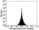
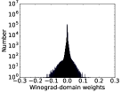
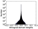
Spatial domain

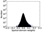
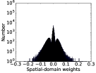
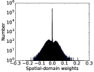
Fig. 2: Weight histogram snapshots of the AlexNet second convolutional layer.

To overcome the problems with fixed regularization coefficients, we propose novel learnable regularization coefficients, i.e., we let regularization coefficients be learnable parameters. Starting from a small initial coefficient value, we learn an accurate model with little regularization. As training goes on, we induce the regularization coefficients to increase gradually so that the performance does not degrade much but we finally have sparse convolutional filters at the end of training. To this end, we replace $\lambda_{\text{WD}}$ and $\lambda_{\text{SD}}$ with $e^{\zeta_{\text{WD}}}$ and $e^{\zeta_{\text{SD}}}$, respectively, and learn $\zeta_{\text{WD}}$ and $\zeta_{\text{SD}}$ instead, for the sake of guaranteeing that the regularization coefficients always positive in training. Then, we include an additional regularization term, i.e., $-\alpha(\zeta_{WD}+\zeta_{SD})$ for $\alpha>0$, which penalizes small regularization coefficients and encourages them to increase in training. As a result, the cost function in (4) is altered into

$$C(\mathcal{X};\mathbf{w},\zeta_{\text{WD}},\zeta_{\text{SD}})=E(\mathcal{X};\mathbf{w})+e^{\zeta_{\text{WD}}}R_{\text{WD}}(\mathbf{w};s_{\text{WD}})\\ +e^{\zeta_{\text{SD}}}R_{\text{SD}}(\mathbf{w};s_{\text{SD}})-\alpha(\zeta_{\text{WD}}+\zeta_{\text{SD}}).$$ (5)

The indicator functions in (2) and (3) are non-differentiable, which is however not a problem when computing the derivatives of (5) in practice for stochastic gradient descent.

(a) Winograd domain	(b) Spatial domain

Fig. 3: Sparse convolutional filters from the AlexNet second convolutional layer, obtained after pruning in either domain.

In Figure 2, we present how the weight histogram (distribution) of the AlexNet second convolutional layer evolves in the Winograd and spatial domains when trained with the proposed cost function in (5). Observe that a part of the weights converges to zero in both domains, which can be pruned at minimal accuracy loss. In Figure 3, we present sparse convolutional filters obtained after pruning either in the Winograd domain and in the spatial domain. They are sampled from the $5\times 5$ filters of the AlexNet second convolutional layer, where we use Winograd convolution of $(r,n)=(5,8)$ in Section 2.

Remark 1.

As observed above, we have presented our algorithms using L2 regularizers. Often L1 norms are used to promote sparsity (e.g., see [23]), but here we suggest using L2 instead, since our goal is to induce small-value weights rather than to drive them to be really zero. The model re-trained with our L2 regularizers is still dense and not sparse before pruning. However, it is jointly regularized to have many small-value weights, which can be pruned at negligible loss, in both domains. The sparsity is actually attained only after pruning its small-value weights in either domain. This is to avoid the fundamental limit of joint sparsity, similar to the uncertainty principle of the Fourier transform [24].

4 Universal compression and dual domain deployment

A universal CNN compression framework is proposed in [9], where CNNs are optimized for and compressed by universal quantization [25] and universal entropy source coding with schemes such as the variants of Lempel–Ziv–Welch [26, 27, 28] and the Burrows–Wheeler transform [29].

Our universal compression pipeline under joint sparsity constraints is summarized in Figure 1. We randomize spatial-domain weights by adding uniform random dithers, and quantize the dithered weights uniformly with interval $\Delta$ by

$$q_{i}=\Delta\cdot\operatorname{round}((a_{i}+U_{i})/\Delta),$$ (6)

where $a_{1},\dots,a_{N_{\text{SD}}}$ are the individual spatial-domain weights of all $L$ layers, and $U_{1},\dots,U_{N_{\text{SD}}}$ are independent and identically distributed uniform random variables with the support of $[-\Delta/2,\Delta/2]$; the rounding yields the closest integer of the input. The weights rounded to zero in (6) are pruned and fixed to be zero in the compressed model. The random dithering values or their random seed are assumed to be known at deployment, and the dithering values are cancelled for the unpruned weights after decompression by $\hat{q}_{i}=q_{i}-U_{i}\cdot 1_{q_{i}\neq 0}$, where $\hat{q}_{i}$ is the final deployed value of weight $a_{i}$ for inference.

For one compressed model, we make the model actually sparse in the spatial domain by pruning small-value weights that are quantized to zero in the spatial domain. The resulting quantized model is sparse in the spatial domain, but it becomes dense in the Winograd domain. To recover the sparsity in the Winograd domain and to compensate the accuracy loss from quantization, we fine-tune the spatial-domain quantization codebook with the Winograd-domain L2 regularizer. Using the cost function $C=E+e^{\zeta_{\text{WD}}}R_{\text{WD}}-\alpha\zeta_{\text{WD}}$ instead of (5), the average gradient is computed for unpruned weights that are quantized to the same value in (6). Then, their shared quantized value in the codebook is updated by gradient descent using the average gradient of them. We emphasize here that the pruned weights in (6) are not fine-tuned and stay zero.

At deployment, the compressed model is decompressed to get unpruned spatial-domain weights. Then, the CNN can be deployed in the spatial domain with the desired sparsity. If we deploy the CNN in the Winograd domain, its convolutional filters are transformed into the Winograd domain, and pruned to the desired sparsity level (see deployment in Figure 1).

5 Experiments

We experiment with our universal CNN pruning and compression scheme on the ResNet-18 model [30] trained for the ImageNet ILSVRC 2012 dataset [31]. As in [20], we modify the original ResNet-18 model by replacing its convolutional layers of stride $2\times 2$ with convolutional layers of stride $1\times 1$ and max-pooling layers, to deploy Winograd convolution for all possible convolutional layers. One difference from [20] is that we place max-pooling after convolution (Conv+Maxpool) instead of placing it before convolution (Maxpool+Conv). Our modification provides better accuracy (see Figure 4).

Table 1: Accuracy and complexity of pruned ResNet-18 models when using different regularization methods.

Regularization (sparsity $s$)	Pruning ratio	(1) Spatial domain		(2) Winograd domain
		Top-1 / Top-5	# MACs	Top-1 / Top-5	# MACs
		accuracy	per image	accuracy	per image
Pre-trained model	-	68.2 / 88.6	2347.1M	68.2 / 88.6	1174.0M
SD (80%)	80%	67.8 / 88.4	837.9M	56.9 / 80.7	467.0M
WD (80%)	80%	44.0 / 70.5	819.7M	68.4 / 88.6	461.9M
WD+SD (80%)	80%	67.8 / 88.5	914.9M	67.8 / 88.5	522.6M

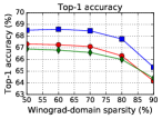
Fig. 4: Accuracy comparison for the pruned ResNet-18 models at different sparsity levels in the Winograd domain.

The Winograd-domain regularizer is applied to all $3\times 3$ convolutional filters. We assume to use Winograd convolution of $(r,n)=(3,4)$ for $3\times 3$ filters (see Section 2). The spatial-domain regularizer is applied to all convolutional and fully-connected layers not only for pruning but also for compression in the spatial domain. We use the Adam optimizer [32] with the learning rate of $1\text{e-}5$ for $500k$ iterations with the batch size of $128$. We set $\alpha=1$ in (5).

In Table 1, we summarize the accuracy and the number of MACs to process one input image for pruned ResNet-18 models. We compare three models obtained with spatial-domain regularization only (SD), Winograd-domain regularization only (WD), and both regularizations (WD+SD). As expected, the proposed regularization method produces its desired sparsity only in the regularized domain. If we prune weights in the other domain, then we suffer from considerable accuracy loss. Using both Winograd-domain and spatial-domain regularizers, we can produce one model that can be sparse and accurate in both domains. In Figure 4, we compare the accuracy of our pruned ResNet-18 models to the ones from [20].

Table 2: Compression results for ResNet-18 and AlexNet.

Model	Method	CR	(1) Spatial domain		(2) Winograd domain
			Top-1 / Top-5	# MACs	Top-1 / Top-5	# MACs
			accuracy	per image	accuracy	per image
ResNet-18	Pre-trained	-	68.2 / 88.6	2347.1M	68.2 / 88.6	1174.0M
	Ours	24.2	67.4 / 88.2	888.6M	67.4 / 88.2	516.4M
AlexNet	Pre-trained	-	56.8 / 80.0	724.4M	56.8 / 80.0	330.0M
	Ours	47.7	56.1 / 79.3	240.0M	56.0 / 79.3	142.6M
	Han et al. [3]	35.0	57.2 / 80.3	301.1M	N/A	N/A
	Guo et al. [16]	N/A	56.9 / 80.0	254.2M	N/A	N/A
	Li et al. [19]	N/A	N/A	N/A	57.3 / N/A	319.8M

Table 2 shows the compression results for the ResNet-18 and AlexNet models. The compression ratio (CR) is the ratio of the original model size to the compressed model size. We note that the previous approaches [3, 16, 19] produce sparse models only in one domain, while our method produces one compressed model that can be used in both domains.

6 Conclusion

We introduced a CNN pruning and compression framework for hardware and/or software platform independent deployment. The proposed scheme produces one compressed model whose convolutional filters can be made sparse in both Winograd and spatial domains without further training. We showed that the proposed method successfully compresses ResNet-18 and AlexNet with compression ratios of $24.2\times$ and $47.7\times$, while reducing their complexity by $4.5\times$ and $5.1\times$, respectively, when using sparse Winograd convolution. Our regularization method can be extended for sparse frequency-domain convolution, which remains as our future work.

References

- [1] Yann LeCun, Yoshua Bengio, and Geoffrey Hinton, “Deep learning,” Nature, vol. 521, no. 7553, pp. 436–444, 2015.
- [2] Vivienne Sze, Yu-Hsin Chen, Tien-Ju Yang, and Joel S Emer, “Efficient processing of deep neural networks: A tutorial and survey,” Proceedings of the IEEE, vol. 105, no. 12, pp. 2295–2329, 2017.
- [3] Song Han, Huizi Mao, and William J Dally, “Deep compression: Compressing deep neural networks with pruning, trained quantization and Huffman coding,” in International Conference on Learning Representations, 2016.
- [4] Yoojin Choi, Mostafa El-Khamy, and Jungwon Lee, “Towards the limit of network quantization,” in International Conference on Learning Representations, 2017.
- [5] Karen Ullrich, Edward Meeds, and Max Welling, “Soft weight-sharing for neural network compression,” in International Conference on Learning Representations, 2017.
- [6] Eirikur Agustsson, Fabian Mentzer, Michael Tschannen, Lukas Cavigelli, Radu Timofte, Luca Benini, and Luc V Gool, “Soft-to-hard vector quantization for end-to-end learning compressible representations,” in Advances in Neural Information Processing Systems, 2017, pp. 1141–1151.
- [7] Dmitry Molchanov, Arsenii Ashukha, and Dmitry Vetrov, “Variational dropout sparsifies deep neural networks,” in International Conference on Machine Learning, 2017, pp. 2498–2507.
- [8] Christos Louizos, Karen Ullrich, and Max Welling, “Bayesian compression for deep learning,” in Advances in Neural Information Processing Systems, 2017, pp. 3290–3300.
- [9] Yoojin Choi, Mostafa El-Khamy, and Jungwon Lee, “Universal deep neural network compression,” in NeurIPS Workshop on Compact Deep Neural Network Representation with Industrial Applications (CDNNRIA), 2018.
- [10] Bin Dai, Chen Zhu, and David Wipf, “Compressing neural networks using the variational information bottleneck,” in International Conference on Machine Learning, 2018.
- [11] Michael Mathieu, Mikael Henaff, and Yann LeCun, “Fast training of convolutional networks through FFTs,” arXiv preprint arXiv:1312.5851, 2013.
- [12] Nicolas Vasilache, Jeff Johnson, Michael Mathieu, Soumith Chintala, Serkan Piantino, and Yann LeCun, “Fast convolutional nets with fbfft: A GPU performance evaluation,” arXiv preprint arXiv:1412.7580, 2014.
- [13] Andrew Lavin and Scott Gray, “Fast algorithms for convolutional neural networks,” in Proceedings of the IEEE Conference on Computer Vision and Pattern Recognition, 2016, pp. 4013–4021.
- [14] Vadim Lebedev and Victor Lempitsky, “Fast convnets using group-wise brain damage,” in Proceedings of the IEEE Conference on Computer Vision and Pattern Recognition, 2016, pp. 2554–2564.
- [15] Wei Wen, Chunpeng Wu, Yandan Wang, Yiran Chen, and Hai Li, “Learning structured sparsity in deep neural networks,” in Advances in Neural Information Processing Systems, 2016, pp. 2074–2082.
- [16] Yiwen Guo, Anbang Yao, and Yurong Chen, “Dynamic network surgery for efficient DNNs,” in Advances In Neural Information Processing Systems, 2016, pp. 1379–1387.
- [17] Ji Lin, Yongming Rao, Jiwen Lu, and Jie Zhou, “Runtime neural pruning,” in Advances in Neural Information Processing Systems, 2017, pp. 2178–2188.
- [18] Jongsoo Park, Sheng Li, Wei Wen, Ping Tak Peter Tang, Hai Li, Yiran Chen, and Pradeep Dubey, “Faster CNNs with direct sparse convolutions and guided pruning,” International Conference on Learning Representations, 2017.
- [19] Sheng Li, Jongsoo Park, and Ping Tak Peter Tang, “Enabling sparse Winograd convolution by native pruning,” arXiv preprint arXiv:1702.08597, 2017.
- [20] Xingyu Liu, Jeff Pool, Song Han, and William J Dally, “Efficient sparse-Winograd convolutional neural networks,” in International Conference on Learning Representations, 2018.
- [21] Shmuel Winograd, Arithmetic Complexity of Computations, vol. 33, SIAM, 1980.
- [22] Richard E Blahut, Fast Algorithms for Signal Processing, Cambridge University Press, 2010.
- [23] Scott Shaobing Chen, David L Donoho, and Michael A Saunders, “Atomic decomposition by basis pursuit,” SIAM Review, vol. 43, no. 1, pp. 129–159, 2001.
- [24] David L Donoho and Philip B Stark, “Uncertainty principles and signal recovery,” SIAM Journal on Applied Mathematics, vol. 49, no. 3, pp. 906–931, 1989.
- [25] Jacob Ziv, “On universal quantization,” IEEE Transactions on Information Theory, vol. 31, no. 3, pp. 344–347, 1985.
- [26] Jacob Ziv and Abraham Lempel, “A universal algorithm for sequential data compression,” IEEE Transactions on Information Theory, vol. 23, no. 3, pp. 337–343, 1977.
- [27] Jacob Ziv and Abraham Lempel, “Compression of individual sequences via variable-rate coding,” IEEE Transactions on Information Theory, vol. 24, no. 5, pp. 530–536, 1978.
- [28] Terry A. Welch, “A technique for high-performance data compression,” Computer, vol. 6, no. 17, pp. 8–19, 1984.
- [29] Michelle Effros, Karthik Visweswariah, Sanjeev R Kulkarni, and Sergio Verdú, “Universal lossless source coding with the Burrows Wheeler transform,” IEEE Transactions on Information Theory, vol. 48, no. 5, pp. 1061–1081, 2002.
- [30] Kaiming He, Xiangyu Zhang, Shaoqing Ren, and Jian Sun, “Deep residual learning for image recognition,” in Proceedings of the IEEE Conference on Computer Vision and Pattern Recognition, 2016, pp. 770–778.
- [31] Olga Russakovsky, Jia Deng, Hao Su, Jonathan Krause, Sanjeev Satheesh, Sean Ma, Zhiheng Huang, Andrej Karpathy, Aditya Khosla, Michael Bernstein, et al., “ImageNet large scale visual recognition challenge,” International Journal of Computer Vision, vol. 115, no. 3, pp. 211–252, 2015.
- [32] Diederik Kingma and Jimmy Ba, “Adam: A method for stochastic optimization,” arXiv preprint arXiv:1412.6980, 2014.