Abstract

We review lattice results related to pion, kaon, $D$-meson, $B$-meson, and nucleon physics with the aim of making them easily accessible to the nuclear and particle physics communities. More specifically, we report on the determination of the light-quark masses, the form factor $f_{+}(0)$ arising in the semileptonic $K\to\pi$ transition at zero momentum transfer, as well as the decay constant ratio $f_{K}/f_{\pi}$ and its consequences for the CKM matrix elements $V_{us}$ and $V_{ud}$. Furthermore, we describe the results obtained on the lattice for some of the low-energy constants of $SU(2)_{L}\times SU(2)_{R}$ and $SU(3)_{L}\times SU(3)_{R}$ Chiral Perturbation Theory. We review the determination of the $B_{K}$ parameter of neutral kaon mixing as well as the additional four $B$ parameters that arise in theories of physics beyond the Standard Model. For the heavy-quark sector, we provide results for $m_{c}$ and $m_{b}$ as well as those for $D$- and $B$-meson decay constants, form factors, and mixing parameters. These are the heavy-quark quantities most relevant for the determination of CKM matrix elements and the global CKM unitarity-triangle fit. We review the status of lattice determinations of the strong coupling constant $\alpha_{s}$. Finally, in this review we have added a new section reviewing results for nucleon matrix elements of the axial, scalar and tensor bilinears, both isovector and flavor diagonal.

1 Introduction

Flavour physics provides an important opportunity for exploring the limits of the Standard Model of particle physics and for constraining possible extensions that go beyond it. As the LHC explores a new energy frontier and as experiments continue to extend the precision frontier, the importance of flavour physics will grow, both in terms of searches for signatures of new physics through precision measurements and in terms of attempts to construct the theoretical framework behind direct discoveries of new particles. Crucial to such searches for new physics is the ability to quantify strong-interaction effects. Large-scale numerical simulations of lattice QCD allow for the computation of these effects from first principles. The scope of the Flavour Lattice Averaging Group (FLAG) is to review the current status of lattice results for a variety of physical quantities that are important for flavour physics. Set up in November 2007, it comprises experts in Lattice Field Theory, Chiral Perturbation Theory and Standard Model phenomenology. Our aim is to provide an answer to the frequently posed question “What is currently the best lattice value for a particular quantity?” in a way that is readily accessible to those who are not expert in lattice methods. This is generally not an easy question to answer; different collaborations use different lattice actions (discretizations of QCD) with a variety of lattice spacings and volumes, and with a range of masses for the $u$- and $d$-quarks. Not only are the systematic errors different, but also the methodology used to estimate these uncertainties varies between collaborations. In the present work, we summarize the main features of each of the calculations and provide a framework for judging and combining the different results. Sometimes it is a single result that provides the “best” value; more often it is a combination of results from different collaborations. Indeed, the consistency of values obtained using different formulations adds significantly to our confidence in the results.

The first three editions of the FLAG review were made public in 2010 [Colangelo:2010et], 2013 [Aoki:2013ldr], and 2016 [Aoki:2016frl] (and will be referred to as FLAG 10, FLAG 13 and FLAG 16, respectively). The third edition reviewed results related to both light ($u$-, $d$- and $s$-), and heavy ($c$- and $b$-) flavours. The quantities related to pion and kaon physics were light-quark masses, the form factor $f_{+}(0)$ arising in semileptonic $K\rightarrow\pi$ transitions (evaluated at zero momentum transfer), the decay constants $f_{K}$ and $f_{\pi}$, the $B_{K}$ parameter from neutral kaon mixing, and the kaon mixing matrix elements of new operators that arise in theories of physics beyond the Standard Model. Their implications for the CKM matrix elements $V_{us}$ and $V_{ud}$ were also discussed. Furthermore, results were reported for some of the low-energy constants of $SU(2)_{L}\times SU(2)_{R}$ and $SU(3)_{L}\times SU(3)_{R}$ Chiral Perturbation Theory. The quantities related to $D$- and $B$-meson physics that were reviewed were the masses of the charm and bottom quarks together with the decay constants, form factors, and mixing parameters of $B$- and $D$-mesons. These are the heavy-light quantities most relevant to the determination of CKM matrix elements and the global CKM unitarity-triangle fit. Last but not least, the current status of lattice results on the QCD coupling $\alpha_{s}$ was reviewed.

In the present paper we provide updated results for all the above-mentioned quantities, but also extend the scope of the review by adding a section on nucleon matrix elements. This presents results for matrix elements of flavor nonsinglet and singlet bilinear operators, including the nucleon axial charge $g_{A}$ and the nucleon sigma terms. These results are relevant for constraining $V_{ud}$, for searches for new physics in neutron decays and other processes, and for dark matter searches. In addition, the section on up and down quark masses has been largely rewritten, replacing previous estimates for $m_{u}$, $m_{d}$, and the mass ratios $R$ and $Q$ that were largely phenomenological with those from lattice QED+QCD calculations. We have also updated the discussion of the phenomenology of isospin-breaking effects in the light meson sector, and their relation to quark masses, with a lattice-centric discussion. A short review of QED in lattice-QCD simulations is also provided, including a discussion of ambiguities arising when attempting to define “physical” quantities in pure QCD.

Our main results are collected in Tabs. 1, 1 and 1. As is clear from the tables, for most quantities there are results from ensembles with different values for $N_{f}$. In most cases, there is reasonable agreement among results with $N_{f}=2$, $2+1$, and $2+1+1$. As precision increases, we may some day be able to distinguish among the different values of $N_{f}$, in which case, presumably $2+1+1$ would be the most realistic. (If isospin violation is critical, then $1+1+1$ or $1+1+1+1$ might be desired.) At present, for some quantities the errors in the $N_{f}=2+1$ results are smaller than those with $N_{f}=2+1+1$ (e.g., for $m_{c}$), while for others the relative size of the errors is reversed. Our suggestion to those using the averages is to take whichever of the $N_{f}=2+1$ or $N_{f}=2+1+1$ results has the smaller error. We do not recommend using the $N_{f}=2$ results, except for studies of the $N_{f}$-dependence of condensates and $\alpha_{s}$, as these have an uncontrolled systematic error coming from quenching the strange quark.

Our plan is to continue providing FLAG updates, in the form of a peer reviewed paper, roughly on a triennial basis. This effort is supplemented by our more frequently updated website http://flag.unibe.ch [FLAG:webpage], where figures as well as pdf-files for the individual sections can be downloaded. The papers reviewed in the present edition have appeared before the closing date 30 September 2018.

Quantity	Sec.	$N_{f}=2+1+1$	Refs.	$N_{f}=2+1$	Refs.	$N_{f}=2$	Refs.
$m_{ud}$[MeV]	3.1.4	$3.410(43)$	[Bazavov:2018omf, Carrasco:2014cwa]	$3.364(41)$	[Blum:2014tka, Durr:2010vn, Durr:2010aw, McNeile:2010ji, Bazavov:2010yq]
$m_{s}$[MeV]	3.1.4	$93.44(68)$	[Bazavov:2018omf, Lytle:2018evc, Carrasco:2014cwa, Chakraborty:2014aca]	$92.0(1.1)$	[Bazavov:2009fk, Durr:2010vn, Durr:2010aw, McNeile:2010ji, Blum:2014tka]
$m_{s}/m_{ud}$	3.1.5	$27.23(10)$	[Bazavov:2017lyh, Carrasco:2014cwa, Bazavov:2014wgs]	$27.42(12)$	[Blum:2014tka, Bazavov:2009fk, Durr:2010vn, Durr:2010aw]
$m_{u}$[MeV]	3.1.6	$2.50(17)$	[Giusti:2017dmp]	$2.27(9)$	[Fodor:2016bgu]
$m_{d}$[MeV]	3.1.6	$4.88(20)$	[Giusti:2017dmp]	$4.67(9)$	[Fodor:2016bgu]
${m_{u}}/{m_{d}}$	3.1.6	$0.513(31)$	[Giusti:2017dmp]	$0.485(19)$	[Fodor:2016bgu]
$\overline{m}_{c}(\mbox{3 GeV})$[GeV]	3.2.2	$0.988(7)$	[Carrasco:2014cwa, Chakraborty:2014aca, Alexandrou:2014sha, Bazavov:2018omf, Lytle:2018evc]	$0.992(6)$	[McNeile:2010ji, Yang:2014sea, Nakayama:2016atf]
$m_{c}/m_{s}$	3.2.3	$11.768(33)$	[Chakraborty:2014aca, Carrasco:2014cwa, Bazavov:2018omf]	$11.82(16)$	[Yang:2014sea, Davies:2009ih]
$\overline{m}_{b}(\overline{m}_{b})$[GeV]	3.3	$4.198(12)$	[Chakraborty:2014aca, Colquhoun:2014ica, Bussone:2016iua, Gambino:2017vkx, Bazavov:2018omf]	$4.164(23)$	[McNeile:2010ji]
$f_{+}(0)$	4.3	$0.9706(27)$	[Bazavov:2013maa, Carrasco:2016kpy]	$0.9677(27)$	[Bazavov:2012cd, Boyle:2015hfa]	$0.9560(57)(62)$	[Lubicz:2009ht]
$f_{K^{\pm}}/f_{\pi^{\pm}}$	4.3	$1.1932(19)$	[Dowdall:2013rya, Carrasco:2014poa, Bazavov:2017lyh]	$1.1917(37)$	[Follana:2007uv, Bazavov:2010hj, Durr:2010hr, Blum:2014tka, Durr:2016ulb, Bornyakov:2016dzn]	$1.205(18)$	[Blossier:2009bx]
$f_{\pi^{\pm}}$[MeV]	4.6			$130.2(8)$	[Follana:2007uv, Bazavov:2010hj, Blum:2014tka]
$f_{K^{\pm}}$[MeV]	4.6	$155.7(3)$	[Dowdall:2013rya, Bazavov:2014wgs, Carrasco:2014poa]	$155.7(7)$	[Follana:2007uv, Bazavov:2010hj, Blum:2014tka]	$157.5(2.4)$	[Blossier:2009bx]
$\Sigma^{1/3}$[MeV]	5.2.2	$286(23)$	[Cichy:2013gja, Alexandrou:2017bzk]	$272(5)$	[Bazavov:2010yq, Borsanyi:2012zv, Durr:2013goa, Boyle:2015exm, Cossu:2016eqs, Aoki:2017paw]	$266(10)$	[Baron:2009wt, Cichy:2013gja, Brandt:2013dua, Engel:2014eea]
${F_{\pi}}/{F}$	5.2.2	$1.077(3)$	[Baron:2011sf]	$1.062(7)$	[Bazavov:2010hj, Beane:2011zm, Borsanyi:2012zv, Durr:2013goa, Boyle:2015exm]	$1.073(15)$	[Frezzotti:2008dr, Baron:2009wt, Brandt:2013dua, Engel:2014eea]
$\bar{\ell}_{3}$	5.2.3	$3.53(26)$	[Baron:2011sf]	$3.07(64)$	[Bazavov:2010hj, Beane:2011zm, Borsanyi:2012zv, Durr:2013goa, Boyle:2015exm]	$3.41(82)$	[Frezzotti:2008dr, Baron:2009wt, Brandt:2013dua]
$\bar{\ell}_{4}$	5.2.3	$4.73(10)$	[Baron:2011sf]	$4.02(45)$	[Bazavov:2010hj, Beane:2011zm, Borsanyi:2012zv, Durr:2013goa, Boyle:2015exm]	$4.40(28)$	[Frezzotti:2008dr, Baron:2009wt, Brandt:2013dua, Gulpers:2015bba]
$\bar{\ell}_{6}$	5.2.3					$15.1(1.2)$	[Frezzotti:2008dr, Brandt:2013dua]
$\hat{B}_{K}$	6.2	$0.717(18)(16)$	[Carrasco:2015pra]	$0.7625(97)$	[Durr:2011ap, Laiho:2011np, Blum:2014tka, Jang:2015sla]	$0.727(22)(12)$	[Bertone:2012cu]
$B_{2}$	6.3	$0.46(1)(3)$	[Carrasco:2015pra]	$0.502(14)$	[Jang:2015sla, Garron:2016mva]	$0.47(2)(1)$	[Bertone:2012cu]
$B_{3}$	6.3	$0.79(2)(4)$	[Carrasco:2015pra]	$0.766(32)$	[Jang:2015sla, Garron:2016mva]	$0.78(4)(2)$	[Bertone:2012cu]
$B_{4}$	6.3	$0.78(2)(4)$	[Carrasco:2015pra]	$0.926(19)$	[Jang:2015sla, Garron:2016mva]	$0.76(2)(2)$	[Bertone:2012cu]
$B_{5}$	6.3	$0.49(3)(3)$	[Carrasco:2015pra]	$0.720(38)$	[Jang:2015sla, Garron:2016mva]	$0.58(2)(2)$	[Bertone:2012cu]

Table 1: Summary of the main results of this review concerning quark masses, light-meson decay constants, LECs, and kaon mixing parameters. These are grouped in terms of $N_{f}$, the number of dynamical quark flavours in lattice simulations. Quark masses and the quark condensate are given in the ${\overline{\mathrm{MS}}}$ scheme at running scale $\mu=2\,\mathrm{Ge\kern-1.00006ptV}$ or as indicated. BSM bag parameters $B_{2,3,4,5}$ are given in the ${\overline{\mathrm{MS}}}$ scheme at scale $\mu=3\,\mathrm{Ge\kern-1.00006ptV}$. Further specifications of the quantities are given in the quoted sections. Results for $N_{f}=2$ quark masses are unchanged since FLAG 16 [Aoki:2016frl]. For each result we list the references that enter the FLAG average or estimate, and we stress again the importance of quoting these original works when referring to FLAG results. From the entries in this column one can also read off the number of results that enter our averages for each quantity. We emphasize that these numbers only give a very rough indication of how thoroughly the quantity in question has been explored on the lattice and recommend consulting the detailed tables and figures in the relevant section for more significant information and for explanations on the source of the quoted errors.

Table 2: Summary of the main results of this review concerning heavy-light mesons and the strong coupling constant. These are grouped in terms of $N_{f}$, the number of dynamical quark flavours in lattice simulations. The quantities listed are specified in the quoted sections. For each result we list the references that enter the FLAG average or estimate, and we stress again the importance of quoting these original works when referring to FLAG results. From the entries in this column one can also read off the number of results that enter our averages for each quantity. We emphasize that these numbers only give a very rough indication of how thoroughly the quantity in question has been explored on the lattice and recommend consulting the detailed tables and figures in the relevant section for more significant information and for explanations on the source of the quoted errors.

Sec.    $N_{f}=2+1$ and $N_{f}=2+1+1$      Refs. $\alpha_{\overline{\rm MS}}^{(5)}(M_{Z})$LABEL:s:alpsumm   $0.1182(8)$     [Bruno:2017gxd, Nakayama:2016atf, Bazavov:2014soa, Chakraborty:2014aca, McNeile:2010ji, Aoki:2009tf, Maltman:2008bx] $\Lambda_{\overline{\rm MS}}^{(5)}$[MeV]LABEL:s:alpsumm   $211(10)$     [Bruno:2017gxd, Nakayama:2016atf, Bazavov:2014soa, Chakraborty:2014aca, McNeile:2010ji, Aoki:2009tf, Maltman:2008bx] $\Lambda_{\overline{\rm MS}}^{(4)}$[MeV]LABEL:s:alpsumm   $294(12)$     [Bruno:2017gxd, Nakayama:2016atf, Bazavov:2014soa, Chakraborty:2014aca, McNeile:2010ji, Aoki:2009tf, Maltman:2008bx] $\Lambda_{\overline{\rm MS}}^{(3)}$[MeV]LABEL:s:alpsumm   $343(12)$     [Bruno:2017gxd, Nakayama:2016atf, Bazavov:2014soa, Chakraborty:2014aca, McNeile:2010ji, Aoki:2009tf, Maltman:2008bx]

Table 3: Summary of the main results of this review concerning nuclear matrix elements, grouped in terms of $N_{f}$, the number of dynamical quark flavours in lattice simulations. The quantities listed are specified in the quoted sections. For each result we list the references that enter the FLAG average or estimate, and we stress again the importance of quoting these original works when referring to FLAG results. From the entries in this column one can also read off the number of results that enter our averages for each quantity. We emphasize that these numbers only give a very rough indication of how thoroughly the quantity in question has been explored on the lattice and recommend consulting the detailed tables and figures in the relevant section for more significant information and for explanations on the source of the quoted errors.

This review is organized as follows. In the remainder of Sec. 1 we summarize the composition and rules of FLAG and discuss general issues that arise in modern lattice calculations. In Sec. 2, we explain our general methodology for evaluating the robustness of lattice results. We also describe the procedures followed for combining results from different collaborations in a single average or estimate (see Sec. 2.2 for our definition of these terms). The rest of the paper consists of sections, each dedicated to a set of closely connected physical quantities. Each of these sections is accompanied by an Appendix with explicatory notes. Finally, in Appendix LABEL:comm we provide a glossary in which we introduce some standard lattice terminology (e.g., concerning the gauge, light-quark and heavy-quark actions), and in addition we summarize and describe the most commonly used lattice techniques and methodologies (e.g., related to renormalization, chiral extrapolations, scale setting).

1.1 FLAG composition, guidelines and rules

FLAG strives to be representative of the lattice community, both in terms of the geographical location of its members and the lattice collaborations to which they belong. We aspire to provide the nuclear- and particle-physics communities with a single source of reliable information on lattice results.

In order to work reliably and efficiently, we have adopted a formal structure and a set of rules by which all FLAG members abide. The collaboration presently consists of an Advisory Board (AB), an Editorial Board (EB), and eight Working Groups (WG). The rôle of the Advisory Board is to provide oversight of the content, procedures, schedule and membership of FLAG, to help resolve disputes, to serve as a source of advice to the EB and to FLAG as a whole, and to provide a critical assessment of drafts. They also give their approval of the final version of the preprint before it is rendered public. The Editorial Board coordinates the activities of FLAG, sets priorities and intermediate deadlines, organizes votes on FLAG procedures, writes the introductory sections, and takes care of the editorial work needed to amalgamate the sections written by the individual working groups into a uniform and coherent review. The working groups concentrate on writing the review of the physical quantities for which they are responsible, which is subsequently circulated to the whole collaboration for critical evaluation.

The current list of FLAG members and their Working Group assignments is:

• Advisory Board (AB): S. Aoki, M. Golterman, R. Van De Water, and A. Vladikas

• Editorial Board (EB): G. Colangelo, A. Jüttner, S. Hashimoto, S.R. Sharpe,

and U. Wenger • Working Groups (coordinator listed first): – Quark masses T. Blum, A. Portelli, and A. Ramos – $V_{us},V_{ud}$ S. Simula, T. Kaneko, and J. N. Simone – LEC S. Dürr, H. Fukaya, and U.M. Heller – $B_{K}$ P. Dimopoulos, G. Herdoiza, and R. Mawhinney – $f_{B_{(s)}}$, $f_{D_{(s)}}$, $B_{B}$ D. Lin, Y. Aoki, and M. Della Morte – $B_{(s)}$, $D$ semileptonic and radiative decays E. Lunghi, D. Becirevic, S. Gottlieb, and C. Pena – $\alpha_{s}$ R. Sommer, R. Horsley, and T. Onogi – NME R. Gupta, S. Collins, A. Nicholson, and H. Wittig The most important FLAG guidelines and rules are the following: • the composition of the AB reflects the main geographical areas in which lattice collaborations are active, with members from America, Asia/Oceania, and Europe; • the mandate of regular members is not limited in time, but we expect that a certain turnover will occur naturally; • whenever a replacement becomes necessary this has to keep, and possibly improve, the balance in FLAG, so that different collaborations, from different geographical areas are represented; • in all working groups the three members must belong to three different lattice collaborations;${}^{,}$ • a paper is in general not reviewed (nor colour-coded, as described in the next section) by any of its authors; • lattice collaborations will be consulted on the colour coding of their calculation; • there are also internal rules regulating our work, such as voting procedures.

For this edition of the FLAG review, we sought the advice of external reviewers once a complete draft of the review was available. For each review section, we have asked one lattice expert (who could be a FLAG alumnus/alumna) and one nonlattice phenomenologist for a critical assessment. This is similar to the procedure followed by the Particle Data Group in the creation of the Review of Particle Physics. The reviewers provide comments and feedback on scientific and stylistic matters. They are not anonymous, and enter into a discussion with the authors of the WG. Our aim with this additional step is to make sure that a wider array of viewpoints enter into the discussions, so as to make this review more useful for its intended audience.

1.2 Citation policy

We draw attention to this particularly important point. As stated above, our aim is to make lattice-QCD results easily accessible to those without lattice expertise, and we are well aware that it is likely that some readers will only consult the present paper and not the original lattice literature. It is very important that this paper not be the only one cited when our results are quoted. We strongly suggest that readers also cite the original sources. In order to facilitate this, in Tabs. 1, 1, and 1, besides summarizing the main results of the present review, we also cite the original references from which they have been obtained. In addition, for each figure we make a bibtex file available on our webpage [FLAG:webpage] which contains the bibtex entries of all the calculations contributing to the FLAG average or estimate. The bibliography at the end of this paper should also make it easy to cite additional papers. Indeed, we hope that the bibliography will be one of the most widely used elements of the whole paper.

1.3 General issues

Several general issues concerning the present review are thoroughly discussed in Sec. 1.1 of our initial 2010 paper [Colangelo:2010et], and we encourage the reader to consult the relevant pages. In the remainder of the present subsection, we focus on a few important points. Though the discussion has been duly updated, it is similar to that of Sec. 1.2 in the previous two reviews [Aoki:2013ldr, Aoki:2016frl], with the addition of comments on the contributions from excited states that are particularly relevant for the new section on NMEs.

The present review aims to achieve two distinct goals: first, to provide a description of the relevant work done on the lattice; and, second, to draw conclusions on the basis of that work, summarizing the results obtained for the various quantities of physical interest.

The core of the information about the work done on the lattice is presented in the form of tables, which not only list the various results, but also describe the quality of the data that underlie them. We consider it important that this part of the review represents a generally accepted description of the work done. For this reason, we explicitly specify the quality requirements used and provide sufficient details in appendices so that the reader can verify the information given in the tables.

On the other hand, the conclusions drawn on the basis of the available lattice results are the responsibility of FLAG alone. Preferring to err on the side of caution, in several cases we draw conclusions that are more conservative than those resulting from a plain weighted average of the available lattice results. This cautious approach is usually adopted when the average is dominated by a single lattice result, or when only one lattice result is available for a given quantity. In such cases, one does not have the same degree of confidence in results and errors as when there is agreement among several different calculations using different approaches. The reader should keep in mind that the degree of confidence cannot be quantified, and it is not reflected in the quoted errors.

Each discretization has its merits, but also its shortcomings. For most topics covered in this review we have an increasingly broad database, and for most quantities lattice calculations based on totally different discretizations are now available. This is illustrated by the dense population of the tables and figures in most parts of this review. Those calculations that do satisfy our quality criteria indeed lead, in almost all cases, to consistent results, confirming universality within the accuracy reached. In our opinion, the consistency between independent lattice results, obtained with different discretizations, methods, and simulation parameters, is an important test of lattice QCD, and observing such consistency also provides further evidence that systematic errors are fully under control.

In the sections dealing with heavy quarks and with $\alpha_{s}$, the situation is not the same. Since the $b$-quark mass can barely be resolved with current lattice spacings, most lattice methods for treating $b$ quarks use effective field theory at some level. This introduces additional complications not present in the light-quark sector. An overview of the issues specific to heavy-quark quantities is given in the introduction of Sec. 8. For $B$- and $D$-meson leptonic decay constants, there already exists a good number of different independent calculations that use different heavy-quark methods, but there are only one or two independent calculations of semileptonic $B$ and $D$ meson form factors and $B$ meson mixing parameters. For $\alpha_{s}$, most lattice methods involve a range of scales that need to be resolved and controlling the systematic error over a large range of scales is more demanding. The issues specific to determinations of the strong coupling are summarized in Sec. LABEL:sec:alpha_s. Number of sea quarks in lattice simulations: Lattice-QCD simulations currently involve two, three or four flavours of dynamical quarks. Most simulations set the masses of the two lightest quarks to be equal, while the strange and charm quarks, if present, are heavier (and tuned to lie close to their respective physical values). Our notation for these simulations indicates which quarks are nondegenerate, e.g., $N_{f}=2+1$ if $m_{u}=m_{d}<m_{s}$ and $N_{f}=2+1+1$ if $m_{u}=m_{d}<m_{s}<m_{c}$. Calculations with $N_{f}=2$, i.e., two degenerate dynamical flavours, often include strange valence quarks interacting with gluons, so that bound states with the quantum numbers of the kaons can be studied, albeit neglecting strange sea-quark fluctuations. The quenched approximation ($N_{f}=0$), in which all sea-quark contributions are omitted, has uncontrolled systematic errors and is no longer used in modern lattice simulations with relevance to phenomenology. Accordingly, we will review results obtained with $N_{f}=2$, $N_{f}=2+1$, and $N_{f}=2+1+1$, but omit earlier results with $N_{f}=0$. The only exception concerns the QCD coupling constant $\alpha_{s}$. Since this observable does not require valence light quarks, it is theoretically well defined also in the $N_{f}=0$ theory, which is simply pure gluodynamics. The $N_{f}$-dependence of $\alpha_{s}$, or more precisely of the related quantity $r_{0}\Lambda_{\overline{\mathrm{MS}}}$, is a theoretical issue of considerable interest; here $r_{0}$ is a quantity with the dimension of length that sets the physical scale, as discussed in Appendix LABEL:sec_scale. We stress, however, that only results with $N_{f}\geq 3$ are used to determine the physical value of $\alpha_{s}$ at a high scale. Lattice actions, simulation parameters, and scale setting: The remarkable progress in the precision of lattice calculations is due to improved algorithms, better computing resources, and, last but not least, conceptual developments. Examples of the latter are improved actions that reduce lattice artifacts and actions that preserve chiral symmetry to very good approximation. A concise characterization of the various discretizations that underlie the results reported in the present review is given in Appendix LABEL:sec_lattice_actions.

Physical quantities are computed in lattice simulations in units of the lattice spacing so that they are dimensionless. For example, the pion decay constant that is obtained from a simulation is $f_{\pi}a$, where $a$ is the spacing between two neighboring lattice sites. (All simulations with results quoted in this review use hypercubic lattices, i.e., with the same spacing in all four Euclidean directions.) To convert these results to physical units requires knowledge of the lattice spacing $a$ at the fixed values of the bare QCD parameters (quark masses and gauge coupling) used in the simulation. This is achieved by requiring agreement between the lattice calculation and experimental measurement of a known quantity, which thus “sets the scale” of a given simulation. A few details on this procedure are provided in Appendix LABEL:sec_scale. Renormalization and scheme dependence: Several of the results covered by this review, such as quark masses, the gauge coupling, and $B$-parameters, are for quantities defined in a given renormalization scheme and at a specific renormalization scale. The schemes employed (e.g., regularization-independent MOM schemes) are often chosen because of their specific merits when combined with the lattice regularization. For a brief discussion of their properties, see Appendix LABEL:sec_match. The conversion of the results obtained in these so-called intermediate schemes to more familiar regularization schemes, such as the ${\overline{\mathrm{MS}}}$-scheme, is done with the aid of perturbation theory. It must be stressed that the renormalization scales accessible in simulations are limited, because of the presence of an ultraviolet (UV) cutoff of $\sim\pi/a$. To safely match to ${\overline{\mathrm{MS}}}$, a scheme defined in perturbation theory, Renormalization Group (RG) running to higher scales is performed, either perturbatively or nonperturbatively (the latter using finite-size scaling techniques). Extrapolations: Because of limited computing resources, lattice simulations are often performed at unphysically heavy pion masses, although results at the physical point have become increasingly common. Further, numerical simulations must be done at nonzero lattice spacing, and in a finite (four-dimensional) volume. In order to obtain physical results, lattice data are obtained at a sequence of pion masses and a sequence of lattice spacings, and then extrapolated to the physical pion mass and to the continuum limit. In principle, an extrapolation to infinite volume is also required. However, for most quantities discussed in this review, finite-volume effects are exponentially small in the linear extent of the lattice in units of the pion mass, and, in practice, one often verifies volume independence by comparing results obtained on a few different physical volumes, holding other parameters fixed. To control the associated systematic uncertainties, these extrapolations are guided by effective theories. For light-quark actions, the lattice-spacing dependence is described by Symanzik’s effective theory [Symanzik:1983dc, Symanzik:1983gh]; for heavy quarks, this can be extended and/or supplemented by other effective theories such as Heavy-Quark Effective Theory (HQET). The pion-mass dependence can be parameterized with Chiral Perturbation Theory ($\chi$PT), which takes into account the Nambu-Goldstone nature of the lowest excitations that occur in the presence of light quarks. Similarly, one can use Heavy-Light Meson Chiral Perturbation Theory (HM$\chi$PT) to extrapolate quantities involving mesons composed of one heavy ($b$ or $c$) and one light quark. One can combine Symanzik’s effective theory with $\chi$PT to simultaneously extrapolate to the physical pion mass and the continuum; in this case, the form of the effective theory depends on the discretization. See Appendix LABEL:sec_ChiPT for a brief description of the different variants in use and some useful references. Finally, $\chi$PT can also be used to estimate the size of finite-volume effects measured in units of the inverse pion mass, thus providing information on the systematic error due to finite-volume effects in addition to that obtained by comparing simulations at different volumes. Excited-state contamination: In all the hadronic matrix elements discussed in this review, the hadron in question is the lightest state with the chosen quantum numbers. This implies that it dominates the required correlation functions as their extent in Euclidean time is increased. Excited-state contributions are suppressed by $e^{-\Delta E\Delta\tau}$, where $\Delta E$ is the gap between the ground and excited states, and $\Delta\tau$ the relevant separation in Euclidean time. The size of $\Delta E$ depends on the hadron in question, and in general is a multiple of the pion mass. In practice, as discussed at length in Sec. LABEL:sec:NME, the contamination of signals due to excited-state contributions is a much more challenging problem for baryons than for the other particles discussed here. This is in part due to the fact that the signal-to-noise ratio drops exponentially for baryons, which reduces the values of $\Delta\tau$ that can be used. Critical slowing down: The lattice spacings reached in recent simulations go down to 0.05 fm or even smaller. In this regime, long autocorrelation times slow down the sampling of the configurations [Antonio:2008zz, Bazavov:2010xr, Schaefer:2010hu, Luscher:2010we, Schaefer:2010qh, Chowdhury:2013mea, Brower:2014bqa, Fukaya:2015ara, DelDebbio:2002xa, Bernard:2003gq]. Many groups check for autocorrelations in a number of observables, including the topological charge, for which a rapid growth of the autocorrelation time is observed with decreasing lattice spacing. This is often referred to as topological freezing. A solution to the problem consists in using open boundary conditions in time [Luscher:2011kk], instead of the more common antiperiodic ones. More recently two other approaches have been proposed, one based on a multiscale thermalization algorithm [Endres:2015yca, Detmold:2018zgk] and another based on defining QCD on a nonorientable manifold [Mages:2015scv]. The problem is also touched upon in Sec. LABEL:s:crit, where it is stressed that attention must be paid to this issue. While large scale simulations with open boundary conditions are already far advanced [Bruno:2014jqa], only one result reviewed here has been obtained with any of the above methods (results for $\alpha_{s}$ from Ref. [Bruno:2017gxd] which use open boundary conditions). It is usually assumed that the continuum limit can be reached by extrapolation from the existing simulations, and that potential systematic errors due to the long autocorrelation times have been adequately controlled. Partially or completely frozen topology would produce a mixture of different $\theta$ vacua, and the difference from the desired $\theta=0$ result may be estimated in some cases using chiral perturbation theory, which gives predictions for the $\theta$-dependence of the physical quantity of interest [Brower:2003yx, Aoki:2007ka]. These ideas have been systematically and successfully tested in various models in [Bautista:2015yza, Bietenholz:2016ymo], and a numerical test on MILC ensembles indicates that the topology dependence for some of the physical quantities reviewed here is small, consistent with theoretical expectations [Bernard:2017npd]. Simulation algorithms and numerical errors: Most of the modern lattice-QCD simulations use exact algorithms such as those of Refs. [Duane:1987de, Clark:2006wp], which do not produce any systematic errors when exact arithmetic is available. In reality, one uses numerical calculations at double (or in some cases even single) precision, and some errors are unavoidable. More importantly, the inversion of the Dirac operator is carried out iteratively and it is truncated once some accuracy is reached, which is another source of potential systematic error. In most cases, these errors have been confirmed to be much less than the statistical errors. In the following we assume that this source of error is negligible. Some of the most recent simulations use an inexact algorithm in order to speed up the computation, though it may produce systematic effects. Currently available tests indicate that errors from the use of inexact algorithms are under control [Bazavov:2012xda].

2 Quality criteria, averaging and error estimation

The essential characteristics of our approach to the problem of rating and averaging lattice quantities have been outlined in our first publication [Colangelo:2010et]. Our aim is to help the reader assess the reliability of a particular lattice result without necessarily studying the original article in depth. This is a delicate issue, since the ratings may make things appear simpler than they are. Nevertheless, it safeguards against the common practice of using lattice results, and drawing physics conclusions from them, without a critical assessment of the quality of the various calculations. We believe that, despite the risks, it is important to provide some compact information about the quality of a calculation. We stress, however, the importance of the accompanying detailed discussion of the results presented in the various sections of the present review.

2.1 Systematic errors and colour code

The major sources of systematic error are common to most lattice calculations. These include, as discussed in detail below, the chiral, continuum, and infinite-volume extrapolations. To each such source of error for which systematic improvement is possible we assign one of three coloured symbols: green star, unfilled green circle (which replaced in Ref. [Aoki:2013ldr] the amber disk used in the original FLAG review [Colangelo:2010et]) or red square. These correspond to the following ratings:

• the parameter values and ranges used to generate the data sets allow for a satisfactory control of the systematic uncertainties;

• the parameter values and ranges used to generate the data sets allow for a reasonable attempt at estimating systematic uncertainties, which however could be improved;

• the parameter values and ranges used to generate the data sets are unlikely to allow for a reasonable control of systematic uncertainties.

The appearance of a red tag, even in a single source of systematic error of a given lattice result, disqualifies it from inclusion in the global average.

Note that in the first two editions [Colangelo:2010et, Aoki:2013ldr], FLAG used the three symbols in order to rate the reliability of the systematic errors attributed to a given result by the paper’s authors. Starting with the previous edition [Aoki:2016frl] the meaning of the symbols has changed slightly—they now rate the quality of a particular simulation, based on the values and range of the chosen parameters, and its aptness to obtain well-controlled systematic uncertainties. They do not rate the quality of the analysis performed by the authors of the publication. The latter question is deferred to the relevant sections of the present review, which contain detailed discussions of the results contributing (or not) to each FLAG average or estimate.

For most quantities the colour-coding system refers to the following sources of systematic errors: (i) chiral extrapolation; (ii) continuum extrapolation; (iii) finite volume. As we will see below, renormalization is another source of systematic uncertainties in several quantities. This we also classify using the three coloured symbols listed above, but now with a different rationale: they express how reliably these quantities are renormalized, from a field-theoretic point of view (namely, nonperturbatively, or with 2-loop or 1-loop perturbation theory).

Given the sophisticated status that the field has attained, several aspects, besides those rated by the coloured symbols, need to be evaluated before one can conclude whether a particular analysis leads to results that should be included in an average or estimate. Some of these aspects are not so easily expressible in terms of an adjustable parameter such as the lattice spacing, the pion mass or the volume. As a result of such considerations, it sometimes occurs, albeit rarely, that a given result does not contribute to the FLAG average or estimate, despite not carrying any red tags. This happens, for instance, whenever aspects of the analysis appear to be incomplete (e.g., an incomplete error budget), so that the presence of inadequately controlled systematic effects cannot be excluded. This mostly refers to results with a statistical error only, or results in which the quoted error budget obviously fails to account for an important contribution.

Of course, any colour coding has to be treated with caution; we emphasize that the criteria are subjective and evolving. Sometimes, a single source of systematic error dominates the systematic uncertainty and it is more important to reduce this uncertainty than to aim for green stars for other sources of error. In spite of these caveats, we hope that our attempt to introduce quality measures for lattice simulations will prove to be a useful guide. In addition, we would like to stress that the agreement of lattice results obtained using different actions and procedures provides further validation.

2.1.1 Systematic effects and rating criteria

The precise criteria used in determining the colour coding are unavoidably time-dependent; as lattice calculations become more accurate, the standards against which they are measured become tighter. For this reason FLAG reassesses criteria with each edition and as a result some of the quality criteria (the one on chiral extrapolation for instance) have been tightened up over time [Colangelo:2010et, Aoki:2013ldr, Aoki:2016frl].

In the following, we present the rating criteria used in the current report. While these criteria apply to most quantities without modification there are cases where they need to be amended or additional criteria need to be defined. For instance, when discussing results obtained in the $\epsilon$-regime of chiral perturbation theory in Sec. 5 the finite volume criterion listed below for the $p$-regime is no longer appropriate. Similarly, the discussion of the strong coupling constant in Sec. LABEL:sec:alpha_s requires tailored criteria for renormalization, perturbative behaviour, and continuum extrapolation. In such cases, the modified criteria are discussed in the respective sections. Apart from only a few exceptions the following colour code applies in the tables:

• Chiral extrapolation:

or two values of $M_{\pi}$ with one lying within 10 MeV of 135MeV (the physical neutral pion mass) and the other one below 200 MeV $\circ$ 200 MeV $\leq M_{\pi,{\mathrm{min}}}\leq$ 400 MeV, with three or more pion masses used in the extrapolation or two values of $M_{\pi}$ with $M_{\pi,{\mathrm{min}}}<$ 200 MeV or a single value of $M_{\pi}$, lying within 10 MeV of 135 MeV (the physical neutral pion mass) $\blacksquare$ otherwise This criterion has changed with respect to the previous edition [Aoki:2016frl]. • Continuum extrapolation: $\bigstar$ at least three lattice spacings and at least two points below 0.1 fm and a range of lattice spacings satisfying $[a_{\mathrm{max}}/a_{\mathrm{min}}]^{2}\geq 2$ $\circ$ at least two lattice spacings and at least one point below 0.1 fm and a range of lattice spacings satisfying $[a_{\mathrm{max}}/a_{\mathrm{min}}]^{2}\geq 1.4$ $\blacksquare$ otherwise It is assumed that the lattice action is $\mathcal{O}(a)$-improved (i.e., the discretization errors vanish quadratically with the lattice spacing); otherwise this will be explicitly mentioned. For unimproved actions an additional lattice spacing is required. This condition is unchanged from Ref. [Aoki:2016frl]. • Finite-volume effects: The finite-volume colour code used for a result is chosen to be the worse of the QCD and the QED codes, as described below. If only QCD is used the QED colour code is ignored. – For QCD: $\bigstar$ $[M_{\pi,\mathrm{min}}/M_{\pi,\mathrm{fid}}]^{2}\exp\{4-M_{\pi,\mathrm{min}}[L(M_{\pi,\mathrm{min}})]_{\mathrm{max}}\}<1$, or at least three volumes $\circ$ $[M_{\pi,\mathrm{min}}/M_{\pi,\mathrm{fid}}]^{2}\exp\{3-M_{\pi,\mathrm{min}}[L(M_{\pi,\mathrm{min}})]_{\mathrm{max}}\}<1$, or at least two volumes $\blacksquare$ otherwise where we have introduced $[L(M_{\pi,\mathrm{min}})]_{\mathrm{max}}$, which is the maximum box size used in the simulations performed at the smallest pion mass $M_{\pi,{\rm min}}$, as well as a fiducial pion mass $M_{\pi,{\rm fid}}$, which we set to 200 MeV (the cutoff value for a green star in the chiral extrapolation). It is assumed here that calculations are in the $p$-regime of chiral perturbation theory, and that all volumes used exceed 2 fm. This condition has been improved between the second [Aoki:2013ldr] and the third [Aoki:2016frl] edition of the FLAG review but remains unchanged since. The rationale for this condition is as follows. Finite volume effects contain the universal factor $\exp\{-L~{}M_{\pi}\}$, and if this were the only contribution a criterion based on the values of $M_{\pi,\textrm{min}}L$ would be appropriate. This is what we used in Ref. [Aoki:2013ldr] (with $M_{\pi,\textrm{min}}L>4$ for $\bigstar$  and $M_{\pi,\textrm{min}}L>3$ for $\circ$). However, as pion masses decrease, one must also account for the weakening of the pion couplings. In particular, 1-loop chiral perturbation theory [Colangelo:2005gd] reveals a behaviour proportional to $M_{\pi}^{2}\exp\{-L~{}M_{\pi}\}$. Our new condition includes this weakening of the coupling, and ensures, for example, that simulations with $M_{\pi,\mathrm{min}}=135~{}{\rm MeV}$ and $L~{}M_{\pi,\mathrm{min}}=3.2$ are rated equivalently to those with $M_{\pi,\mathrm{min}}=200~{}{\rm MeV}$ and $L~{}M_{\pi,\mathrm{min}}=4$. – For QED (where applicable): $\bigstar$ $1/([M_{\pi,\mathrm{min}}L(M_{\pi,\mathrm{min}})]_{\mathrm{max}})^{n_{\mathrm{min}}}<0.02$, or at least four volumes $\circ$ $1/([M_{\pi,\mathrm{min}}L(M_{\pi,\mathrm{min}})]_{\mathrm{max}})^{n_{\mathrm{min}}}<0.04$, or at least three volumes $\blacksquare$ otherwise Because of the infrared-singular structure of QED, electromagnetic finite-volume effects decay only like a power of the inverse spatial extent. In several cases like mass splittings [Borsanyi:2014jba, Davoudi:2014qua] or leptonic decays [Lubicz:2016xro], the leading corrections are known to be universal, i.e., independent of the structure of the involved hadrons. In such cases, the leading universal effects can be directly subtracted exactly from the lattice data. We denote $n_{\mathrm{min}}$ the smallest power of $\frac{1}{L}$ at which such a subtraction cannot be done. In the widely used finite-volume formulation $\mathrm{QED}_{L}$, one always has $n_{\mathrm{min}}\leq 3$ due to the nonlocality of the theory [Davoudi:2018qpl]. While the QCD criteria have not changed with respect to Ref. [Aoki:2016frl] the QED criteria are new. They are used here only in Sec. 3. • Isospin breaking effects (where applicable): $\bigstar$ all leading isospin breaking effects are included in the lattice calculation $\circ$ isospin breaking effects are included using the electro-quenched approximation $\blacksquare$ otherwise This criterion is used for quantities which are breaking isospin symmetry or which can be determined at the sub-percent accuracy where isospin breaking effects, if not included, are expected to be the dominant source of uncertainty. In the current edition, this criterion is only used for the up and down quark masses, and related quantities ($\epsilon$, $Q^{2}$ and $R^{2}$). The criteria for isospin breaking effects feature for the first time in the FLAG review. • Renormalization (where applicable): $\bigstar$ nonperturbative $\circ$ 1-loop perturbation theory or higher with a reasonable estimate of truncation errors $\blacksquare$ otherwise In Ref. [Colangelo:2010et], we assigned a red square to all results which were renormalized at 1-loop in perturbation theory. In Ref. [Aoki:2013ldr], we decided that this was too restrictive, since the error arising from renormalization constants, calculated in perturbation theory at 1-loop, is often estimated conservatively and reliably. We did not change these criteria since. • Renormalization Group (RG) running (where applicable): For scale-dependent quantities, such as quark masses or $B_{K}$, it is essential that contact with continuum perturbation theory can be established. Various different methods are used for this purpose (cf. Appendix LABEL:sec_match): Regularization-independent Momentum Subtraction (RI/MOM), the Schrödinger functional, and direct comparison with (resummed) perturbation theory. Irrespective of the particular method used, the uncertainty associated with the choice of intermediate renormalization scales in the construction of physical observables must be brought under control. This is best achieved by performing comparisons between nonperturbative and perturbative running over a reasonably broad range of scales. These comparisons were initially only made in the Schrödinger functional approach, but are now also being performed in RI/MOM schemes. We mark the data for which information about nonperturbative running checks is available and give some details, but do not attempt to translate this into a colour code. The pion mass plays an important role in the criteria relevant for chiral extrapolation and finite volume. For some of the regularizations used, however, it is not a trivial matter to identify this mass. In the case of twisted-mass fermions, discretization effects give rise to a mass difference between charged and neutral pions even when the up- and down-quark masses are equal: the charged pion is found to be the heavier of the two for twisted-mass Wilson fermions (cf. Ref. [Boucaud:2007uk]). In early works, typically referring to $N_{f}=2$ simulations (e.g., Refs. [Boucaud:2007uk] and [Baron:2009wt]), chiral extrapolations are based on chiral perturbation theory formulae which do not take these regularization effects into account. After the importance of accounting for isospin breaking when doing chiral fits was shown in Ref. [Bar:2010jk], later works, typically referring to $N_{f}=2+1+1$ simulations, have taken these effects into account [Carrasco:2014cwa]. We use $M_{\pi^{\pm}}$ for $M_{\pi,\mathrm{min}}$ in the chiral-extrapolation rating criterion. On the other hand, we identify $M_{\pi,\mathrm{min}}$ with the root mean square (RMS) of $M_{\pi^{+}}$, $M_{\pi^{-}}$ and $M_{\pi^{0}}$ in the finite-volume rating criterion. In the case of staggered fermions, discretization effects give rise to several light states with the quantum numbers of the pion. The mass splitting among these “taste” partners represents a discretization effect of $\mathcal{O}(a^{2})$, which can be significant at large lattice spacings but shrinks as the spacing is reduced. In the discussion of the results obtained with staggered quarks given in the following sections, we assume that these artifacts are under control. We conservatively identify $M_{\pi,\mathrm{min}}$ with the root mean square (RMS) average of the masses of all the taste partners, both for chiral-extrapolation and finite-volume criteria. The strong coupling $\alpha_{s}$ is computed in lattice QCD with methods differing substantially from those used in the calculations of the other quantities discussed in this review. Therefore, we have established separate criteria for $\alpha_{s}$ results, which will be discussed in Sec. LABEL:s:crit. In the new section on nuclear matrix elements, Sec. LABEL:sec:NME, an additional criterion has been introduced. This concerns the level of control over contamination from excited states, which is a more challenging issue for nucleons than for mesons. In addition, the chiral-extrapolation criterion in this section is somewhat stricter than that given above.

2.1.2 Heavy-quark actions

For the $b$ quark, the discretization of the heavy-quark action follows a very different approach from that used for light flavours. There are several different methods for treating heavy quarks on the lattice, each with its own issues and considerations. Most of these methods use Effective Field Theory (EFT) at some point in the computation, either via direct simulation of the EFT, or by using EFT as a tool to estimate the size of cutoff errors, or by using EFT to extrapolate from the simulated lattice quark masses up to the physical $b$-quark mass. Because of the use of an EFT, truncation errors must be considered together with discretization errors.

The charm quark lies at an intermediate point between the heavy and light quarks. In our earlier reviews, the calculations involving charm quarks often treated it using one of the approaches adopted for the $b$ quark. Since the last report [Aoki:2016frl], however, we found more recent calculations to simulate the charm quark using light-quark actions. This has become possible thanks to the increasing availability of dynamical gauge field ensembles with fine lattice spacings. But clearly, when charm quarks are treated relativistically, discretization errors are more severe than those of the corresponding light-quark quantities.

In order to address these complications, we add a new heavy-quark treatment category to the rating system. The purpose of this criterion is to provide a guideline for the level of action and operator improvement needed in each approach to make reliable calculations possible, in principle.

A description of the different approaches to treating heavy quarks on the lattice is given in Appendix LABEL:app:HQactions, including a discussion of the associated discretization, truncation, and matching errors. For truncation errors we use HQET power counting throughout, since this review is focused on heavy-quark quantities involving $B$ and $D$ mesons rather than bottomonium or charmonium quantities. Here we describe the criteria for how each approach must be implemented in order to receive an acceptable ( ✓) rating for both the heavy-quark actions and the weak operators. Heavy-quark implementations without the level of improvement described below are rated not acceptable ($\blacksquare$). The matching is evaluated together with renormalization, using the renormalization criteria described in Sec. 2.1.1. We emphasize that the heavy-quark implementations rated as acceptable and described below have been validated in a variety of ways, such as via phenomenological agreement with experimental measurements, consistency between independent lattice calculations, and numerical studies of truncation errors. These tests are summarized in Sec. 8. Relativistic heavy-quark actions:  ✓   at least tree-level $\mathcal{O}(a)$ improved action and weak operators This is similar to the requirements for light-quark actions. All current implementations of relativistic heavy-quark actions satisfy this criterion. NRQCD:  ✓   tree-level matched through $\mathcal{O}(1/m_{h})$ and improved through $\mathcal{O}(a^{2})$ The current implementations of NRQCD satisfy this criterion, and also include tree-level corrections of $\mathcal{O}(1/m_{h}^{2})$ in the action. HQET:  ✓   tree-level matched through $\mathcal{O}(1/m_{h})$ with discretization errors starting at $\mathcal{O}(a^{2})$ The current implementation of HQET by the ALPHA collaboration satisfies this criterion, since both action and weak operators are matched nonperturbatively through $\mathcal{O}(1/m_{h})$. Calculations that exclusively use a static-limit action do not satisfy this criterion, since the static-limit action, by definition, does not include $1/m_{h}$ terms. We therefore include static computations in our final estimates only if truncation errors (in $1/m_{h}$) are discussed and included in the systematic uncertainties. Light-quark actions for heavy quarks:  ✓   discretization errors starting at $\mathcal{O}(a^{2})$ or higher This applies to calculations that use the tmWilson action, a nonperturbatively improved Wilson action, domain wall fermions or the HISQ action for charm-quark quantities. It also applies to calculations that use these light quark actions in the charm region and above together with either the static limit or with an HQET-inspired extrapolation to obtain results at the physical $b$-quark mass. In these cases, the continuum-extrapolation criteria described earlier must be applied to the entire range of heavy-quark masses used in the calculation.

2.1.3 Conventions for the figures

For a coherent assessment of the present situation, the quality of the data plays a key role, but the colour coding cannot be carried over to the figures. On the other hand, simply showing all data on equal footing might give the misleading impression that the overall consistency of the information available on the lattice is questionable. Therefore, in the figures we indicate the quality of the data in a rudimentary way, using the following symbols:

• corresponds to results included in the average or estimate (i.e., results that contribute to the black square below);

• corresponds to results that are not included in the average but pass all quality criteria;

• corresponds to all other results;

• corresponds to FLAG averages or estimates; they are also highlighted by a gray vertical band.

The reason for not including a given result in the average is not always the same: the result may fail one of the quality criteria; the paper may be unpublished; it may be superseded by newer results; or it may not offer a complete error budget.

Symbols other than squares are used to distinguish results with specific properties and are always explained in the caption.

Often, nonlattice data are also shown in the figures for comparison. For these we use the following symbols:

• corresponds to nonlattice results;

• corresponds to Particle Data Group (PDG) results.

2.2 Averages and estimates

FLAG results of a given quantity are denoted either as averages or as estimates. Here we clarify this distinction. To start with, both averages and estimates are based on results without any red tags in their colour coding. For many observables there are enough independent lattice calculations of good quality, with all sources of error (not merely those related to the colour-coded criteria), as analyzed in the original papers, appearing to be under control. In such cases, it makes sense to average these results and propose such an average as the best current lattice number. The averaging procedure applied to this data and the way the error is obtained is explained in detail in Sec. 2.3. In those cases where only a sole result passes our rating criteria (colour coding), we refer to it as our FLAG average, provided it also displays adequate control of all other sources of systematic uncertainty.

On the other hand, there are some cases in which this procedure leads to a result that, in our opinion, does not cover all uncertainties. Systematic errors are by their nature often subjective and difficult to estimate, and may thus end up being underestimated in one or more results that receive green symbols for all explicitly tabulated criteria. Adopting a conservative policy, in these cases we opt for an estimate (or a range), which we consider as a fair assessment of the knowledge acquired on the lattice at present. This estimate is not obtained with a prescribed mathematical procedure, but reflects what we consider the best possible analysis of the available information. The hope is that this will encourage more detailed investigations by the lattice community.

There are two other important criteria that also play a role in this respect, but that cannot be colour coded, because a systematic improvement is not possible. These are: i) the publication status, and ii) the number of sea-quark flavours $N_{f}$. As far as the former criterion is concerned, we adopt the following policy: we average only results that have been published in peer-reviewed journals, i.e., they have been endorsed by referee(s). The only exception to this rule consists in straightforward updates of previously published results, typically presented in conference proceedings. Such updates, which supersede the corresponding results in the published papers, are included in the averages. Note that updates of earlier results rely, at least partially, on the same gauge-field-configuration ensembles. For this reason, we do not average updates with earlier results. Nevertheless, all results are listed in the tables, and their publication status is identified by the following symbols:

• Publication status

A  published or plain update of published results P  preprint C  conference contribution

In the present edition, the publication status on the 30th of September 2018 is relevant. If the paper appeared in print after that date, this is accounted for in the bibliography, but does not affect the averages.

As noted above, in this review we present results from simulations with $N_{f}=2$, $N_{f}=2+1$ and $N_{f}=2+1+1$ (except for $r_{0}\Lambda_{\overline{\mathrm{MS}}}$ where we also give the $N_{f}=0$ result). We are not aware of an a priori way to quantitatively estimate the difference between results produced in simulations with a different number of dynamical quarks. We therefore average results at fixed $N_{f}$ separately; averages of calculations with different $N_{f}$ are not provided.

To date, no significant differences between results with different values of $N_{f}$ have been observed in the quantities listed in Tabs. 1, 1, and 1. In the future, as the accuracy and the control over systematic effects in lattice calculations increases, it will hopefully be possible to see a difference between results from simulations with $N_{f}=2$ and $N_{f}=2+1$, and thus determine the size of the Zweig-rule violations related to strange-quark loops. This is a very interesting issue per se, and one which can be quantitatively addressed only with lattice calculations.

The question of differences between results with $N_{f}=2+1$ and $N_{f}=2+1+1$ is more subtle. The dominant effect of including the charm sea quark is to shift the lattice scale, an effect that is accounted for by fixing this scale nonperturbatively using physical quantities. For most of the quantities discussed in this review, it is expected that residual effects are small in the continuum limit, suppressed by $\alpha_{s}(m_{c})$ and powers of $\Lambda^{2}/m_{c}^{2}$. Here $\Lambda$ is a hadronic scale that can only be roughly estimated and depends on the process under consideration. Note that the $\Lambda^{2}/m_{c}^{2}$ effects have been addressed in Refs. [Bruno:2014ufa, Athenodorou:2018wpk]. Assuming that such effects are small, it might be reasonable to average the results from $N_{f}=2+1$ and $N_{f}=2+1+1$ simulations.

2.3 Averaging procedure and error analysis

In the present report, we repeatedly average results obtained by different collaborations, and estimate the error on the resulting averages. Here we provide details on how averages are obtained.

2.3.1 Averaging — generic case

We follow the procedure of the previous two editions [Aoki:2013ldr, Aoki:2016frl], which we describe here in full detail.

One of the problems arising when forming averages is that not all of the data sets are independent. In particular, the same gauge-field configurations, produced with a given fermion discretization, are often used by different research teams with different valence-quark lattice actions, obtaining results that are not really independent. Our averaging procedure takes such correlations into account.

Consider a given measurable quantity $Q$, measured by $M$ distinct, not necessarily uncorrelated, numerical experiments (simulations). The result of each of these measurement is expressed as

$$Q_{i}\,\,=\,\,x_{i}\,\pm\,\sigma^{(1)}_{i}\pm\,\sigma^{(2)}_{i}\pm\cdots\pm\,\sigma^{(E)}_{i}\,\,\,,$$ (1)

where $x_{i}$ is the value obtained by the $i^{\rm th}$ experiment ($i=1,\cdots,M$) and $\sigma^{(k)}_{i}$ (for $k=1,\cdots,E$) are the various errors. Typically $\sigma^{(1)}_{i}$ stands for the statistical error and $\sigma^{(\alpha)}_{i}$ ($\alpha\geq 2$) are the different systematic errors from various sources. For each individual result, we estimate the total error $\sigma_{i}$ by adding statistical and systematic errors in quadrature:

$$Q_{i}\,\, = \,\,x_{i}\,\pm\,\sigma_{i}\,\,\,,$$

$$\sigma_{i}\,\, \equiv \,\,\sqrt{\sum_{\alpha=1}^{E}{\hbox{$\left[\vbox to0.0pt{}\right.\n@space$}}\sigma^{(\alpha)}_{i}{\hbox{$\left]\vbox to0.0pt{}\right.\n@space$}}^{2}}\,\,\,.$$ (2)

With the weight factor of each total error estimated in standard fashion,

$$\omega_{i}\,\,=\,\,\dfrac{\sigma_{i}^{-2}}{\sum_{i=1}^{M}\sigma_{i}^{-2}}\,\,\,,$$ (3)

the central value of the average over all simulations is given by

$$x_{\rm av}\,\, = \,\,\sum_{i=1}^{M}x_{i}\,\omega_{i}\,\,.$$ (4)

The above central value corresponds to a $\chi_{\rm min}^{2}$ weighted average, evaluated by adding statistical and systematic errors in quadrature. If the fit is not of good quality ($\chi_{\rm min}^{2}/{\rm dof}>1$), the statistical and systematic error bars are stretched by a factor $S=\sqrt{\chi^{2}/{\rm dof}}$.

Next, we examine error budgets for individual calculations and look for potentially correlated uncertainties. Specific problems encountered in connection with correlations between different data sets are described in the text that accompanies the averaging. If there is reason to believe that a source of error is correlated between two calculations, a $100\%$ correlation is assumed. The correlation matrix $C_{ij}$ for the set of correlated lattice results is estimated by a prescription due to Schmelling [Schmelling:1994pz]. This consists in defining

$$\sigma_{i;j}\,\,=\,\,\sqrt{{\sum_{\alpha}}^{\prime}{\hbox{$\left[\vbox to0.0pt{}\right.\n@space$}}\sigma_{i}^{(\alpha)}{\hbox{$\left]\vbox to0.0pt{}\right.\n@space$}}^{2}}\,\,\,,$$ (5)

with $\sum_{\alpha}^{\prime}$ running only over those errors of $x_{i}$ that are correlated with the corresponding errors of the measurement $x_{j}$. This expresses the part of the uncertainty in $x_{i}$ that is correlated with the uncertainty in $x_{j}$. If no such correlations are known to exist, then we take $\sigma_{i;j}=0$. The diagonal and off-diagonal elements of the correlation matrix are then taken to be

$$C_{ii}\,\, = \,\,\sigma_{i}^{2}\qquad\qquad(i=1,\cdots,M)\,\,\,,$$

$$C_{ij}\,\, = \,\,\sigma_{i;j}\,\sigma_{j;i}\qquad\qquad(i\neq j)\,\,\,.$$ (6)

Finally, the error of the average is estimated by

$$\sigma^{2}_{\rm av}\,\,=\,\,\sum_{i=1}^{M}\sum_{j=1}^{M}\omega_{i}\,\omega_{j}\,C_{ij}\,\,,$$ (7)

and the FLAG average is

$$Q_{\rm av}\,\,=\,\,x_{\rm av}\,\pm\,\sigma_{\rm av}\,\,\,.$$ (8)

2.3.2 Nested averaging

We have encountered one case where the correlations between results are more involved, and a nested averaging scheme is required. This concerns the $B$-meson bag parameters discussed in Sec. 8.2. In the following, we describe the details of the nested averaging scheme. This is an updated version of the section added in the web update of the FLAG 16 report.

The issue arises for a quantity $Q$ that is given by a ratio, $Q=Y/Z$. In most simulations, both $Y$ and $Z$ are calculated, and the error in $Q$ can be obtained in each simulation in the standard way. However, in other simulations only $Y$ is calculated, with $Z$ taken from a global average of some type. The issue to be addressed is that this average value $\overline{Z}$ has errors that are correlated with those in $Q$.

In the example that arises in Sec. 8.2, $Q=B_{B}$, $Y=B_{B}f_{B}^{2}$ and $Z=f_{B}^{2}$. In one of the simulations that contribute to the average, $Z$ is replaced by $\overline{Z}$, the PDG average for $f_{B}^{2}$ [Rosner:2015wva] (obtained with an averaging procedure similar to that used by FLAG). This simulation is labeled with $i=1$, so that

$$Q_{1}=\frac{Y_{1}}{\overline{Z}}.$$ (9)

The other simulations have results labeled $Q_{j}$, with $j\geq 2$. In this set up, the issue is that $\overline{Z}$ is correlated with the $Q_{j}$, $j\geq 2$.

We begin by decomposing the error in $Q_{1}$ in the same schematic form as above,

$$Q_{1}=x_{1}\pm\frac{\sigma_{Y_{1}}^{(1)}}{\overline{Z}}\pm\frac{\sigma_{Y_{1}}^{(2)}}{\overline{Z}}\pm\cdots\pm\frac{\sigma_{Y_{1}}^{(E)}}{\overline{Z}}\pm\frac{Y_{1}\sigma_{\overline{Z}}}{\overline{Z}^{2}}.$$ (10)

Here the last term represents the error propagating from that in $\overline{Z}$, while the others arise from errors in $Y_{1}$. For the remaining $Q_{j}$ ($j\geq 2$) the decomposition is as in Eq. (1). The total error of $Q_{1}$ then reads

$$\sigma_{1}^{2}=\left(\frac{\sigma_{Y_{1}}^{(1)}}{\overline{Z}}\right)^{2}+\left(\frac{\sigma_{Y_{1}}^{(2)}}{\overline{Z}}\right)^{2}+\cdots+\left(\frac{\sigma_{Y_{1}}^{(E)}}{\overline{Z}}\right)^{2}+\left(\frac{Y_{1}}{\overline{Z}^{2}}\right)^{2}\sigma_{\overline{Z}}^{2},$$ (11)

while that for the $Q_{j}$ ($j\geq 2$) is

$$\sigma_{j}^{2}=\left(\sigma_{j}^{(1)}\right)^{2}+\left(\sigma_{j}^{(2)}\right)^{2}+\cdots+\left(\sigma_{j}^{(E)}\right)^{2}.$$ (12)

Correlations between $Q_{j}$ and $Q_{k}$ ($j,k\geq 2$) are taken care of by Schmelling’s prescription, as explained above. What is new here is how the correlations between $Q_{1}$ and $Q_{j}$ ($j\geq 2$) are taken into account.

To proceed, we recall from Eq. (7) that $\sigma_{\overline{Z}}$ is given by

$$\sigma_{\overline{Z}}^{2}=\sum_{{i^{\prime}},{j^{\prime}}=1}^{M^{\prime}}\omega[Z]_{i^{\prime}}\omega[Z]_{j^{\prime}}C[Z]_{i^{\prime}j^{\prime}}.$$ (13)

Here the indices $i^{\prime}$ and $j^{\prime}$ run over the $M^{\prime}$ simulations that contribute to $\overline{Z}$, which, in general, are different from those contributing to the results for $Q$. The weights $\omega[Z]$ and correlation matrix $C[Z]$ are given an explicit argument $Z$ to emphasize that they refer to the calculation of this quantity and not to that of $Q$. $C[Z]$ is calculated using the Schmelling prescription [Eqs. (5)–(7)] in terms of the errors, $\sigma[Z]_{i^{\prime}}^{(\alpha)}$, taking into account the correlations between the different calculations of $Z$.

We now generalize Schmelling’s prescription for $\sigma_{i;j}$, Eq. (5), to that for $\sigma_{1;k}$ ($k\geq 2$), i.e., the part of the error in $Q_{1}$ that is correlated with $Q_{k}$. We take

$$\sigma_{1;k}\,\,=\,\,\sqrt{\frac{1}{\overline{Z}^{2}}\sum^{\prime}_{(\alpha)\leftrightarrow k}{\hbox{$\left[\vbox to0.0pt{}\right.\n@space$}}\sigma_{Y_{1}}^{(\alpha)}{\hbox{$\left]\vbox to0.0pt{}\right.\n@space$}}^{2}+\frac{Y_{1}^{2}}{\overline{Z}^{4}}\sum_{i^{\prime},j^{\prime}}^{M^{\prime}}\omega[Z]_{i^{\prime}}\omega[Z]_{j^{\prime}}C[Z]_{i^{\prime}j^{\prime}\leftrightarrow k}}\,\,\,.$$ (14)

The first term under the square root sums those sources of error in $Y_{1}$ that are correlated with $Q_{k}$. Here we are using a more explicit notation from that in Eq. (5), with $(\alpha)\leftrightarrow k$ indicating that the sum is restricted to the values of $\alpha$ for which the error $\sigma_{Y_{1}}^{(\alpha)}$ is correlated with $Q_{k}$. The second term accounts for the correlations within $\overline{Z}$ with $Q_{k}$, and is the nested part of the present scheme. The new matrix $C[Z]_{i^{\prime}j^{\prime}\leftrightarrow k}$ is a restriction of the full correlation matrix $C[Z]$, and is defined as follows. Its diagonal elements are given by

$$C[Z]_{i^{\prime}i^{\prime}\leftrightarrow k}\,\, = \,\,(\sigma[Z]_{i^{\prime}\leftrightarrow k})^{2}\qquad\qquad(i^{\prime}=1,\cdots,M^{\prime})\,\,\,,$$ (15)

$$(\sigma[Z]_{i^{\prime}\leftrightarrow k})^{2} = \sum^{\prime}_{(\alpha)\leftrightarrow k}(\sigma[Z]_{i^{\prime}}^{(\alpha)})^{2},$$ (16)

where the summation $\sum^{\prime}_{(\alpha)\leftrightarrow k}$ over $(\alpha)$ is restricted to those $\sigma[Z]_{i^{\prime}}^{(\alpha)}$ that are correlated with $Q_{k}$. The off-diagonal elements are

$$C[Z]_{i^{\prime}j^{\prime}\leftrightarrow k}\,\, = \,\,\sigma[Z]_{i^{\prime};j^{\prime}\leftrightarrow k}\,\sigma[Z]_{j^{\prime};i^{\prime}\leftrightarrow k}\qquad\qquad(i^{\prime}\neq j^{\prime})\,\,\,,$$ (17)

$$\sigma[Z]_{i^{\prime};j^{\prime}\leftrightarrow k} = \sqrt{\sum^{\prime}_{(\alpha)\leftrightarrow j^{\prime}k}(\sigma[Z]_{i^{\prime}}^{(\alpha)})^{2}},$$ (18)

where the summation $\sum^{\prime}_{(\alpha)\leftrightarrow j^{\prime}k}$ over $(\alpha)$ is restricted to $\sigma[Z]_{i^{\prime}}^{(\alpha)}$ that are correlated with both $Z_{j^{\prime}}$ and $Q_{k}$.

The last quantity that we need to define is $\sigma_{k;1}$.

$$\sigma_{k;1}\,\,=\,\,\sqrt{\sum^{\prime}_{(\alpha)\leftrightarrow 1}{\hbox{$\left[\vbox to0.0pt{}\right.\n@space$}}\sigma_{k}^{(\alpha)}{\hbox{$\left]\vbox to0.0pt{}\right.\n@space$}}^{2}}\,\,\,,$$ (19)

where the summation $\sum^{\prime}_{(\alpha)\leftrightarrow 1}$ is restricted to those $\sigma_{k}^{(\alpha)}$ that are correlated with one of the terms in Eq. (11).

In summary, we construct the correlation matrix $C_{ij}$ using Eq. (6), as in the generic case, except the expressions for $\sigma_{1;k}$ and $\sigma_{k;1}$ are now given by Eqs. (14) and (19), respectively. All other $\sigma_{i;j}$ are given by the original Schmelling prescription, Eq. (5). In this way we extend the philosophy of Schmelling’s approach while accounting for the more involved correlations.

3 Quark masses

Authors: T. Blum, A. Portelli, A. Ramos

Quark masses are fundamental parameters of the Standard Model. An accurate determination of these parameters is important for both phenomenological and theoretical applications. The bottom- and charm-quark masses, for instance, are important sources of parametric uncertainties in several Higgs decay modes. The up-, down- and strange-quark masses govern the amount of explicit chiral symmetry breaking in QCD. From a theoretical point of view, the values of quark masses provide information about the flavour structure of physics beyond the Standard Model. The Review of Particle Physics of the Particle Data Group contains a review of quark masses [Manohar_and_Sachrajda], which covers light as well as heavy flavours. Here we also consider light- and heavy-quark masses, but focus on lattice results and discuss them in more detail. We do not discuss the top quark, however, because it decays weakly before it can hadronize, and the nonperturbative QCD dynamics described by present day lattice simulations is not relevant. The lattice determination of light- (up, down, strange), charm- and bottom-quark masses is considered below in Secs. 3.1, 3.2, and 3.3, respectively.

Quark masses cannot be measured directly in experiment because quarks cannot be isolated, as they are confined inside hadrons. From a theoretical point of view, in QCD with $N_{f}$ flavours, a precise definition of quark masses requires one to choose a particular renormalization scheme. This renormalization procedure introduces a renormalization scale $\mu$, and quark masses depend on this renormalization scale according to the Renormalization Group (RG) equations. In mass-independent renormalization schemes the RG equations reads

$$\mu\frac{{\rm d}\bar{m}_{i}(\mu)}{{\rm d}{\mu}}=\bar{m}_{i}(\mu)\tau(\bar{g})\,,$$ (20)

where the function $\tau(\bar{g})$ is the anomalous dimension, which depends only on the value of the strong coupling $\alpha_{s}=\bar{g}^{2}/(4\pi)$. Note that in QCD $\tau(\bar{g})$ is the same for all quark flavours. The anomalous dimension is scheme dependent, but its perturbative expansion

$$\tau(\bar{g})\raisebox{-0.43057pt}{ $\stackrel{{\scriptstyle\small{\bar{g}\to 0}}}{{\sim}}$}-\bar{g}^{2}\left(d_{0}+d_{1}\bar{g}^{2}+\dots\right)$$ (21)

has a leading coefficient $d_{0}=8/(4\pi)^{2}$, which is scheme independent. Equation (20), being a first order differential equation, can be solved exactly by using Eq. (21) as boundary condition. The formal solution of the RG equation reads

$$M_{i}=\bar{m}_{i}(\mu)[2b_{0}\bar{g}^{2}(\mu)]^{-d_{0}/(2b_{0})}\exp\left\{-\int_{0}^{\bar{g}(\mu)}{\rm d}x\,\left[\frac{\tau(x)}{\beta(x)}-\frac{d_{0}}{b_{0}x}\right]\right\}\,,$$ (22)

where $b_{0}=(11-2N_{f}/3)/(4\pi)^{2}$ is the universal leading perturbative coefficient in the expansion of the $\beta$-function $\beta(\bar{g})$. The renormalization group invariant (RGI) quark masses $M_{i}$ are formally integration constants of the RG Eq. (20). They are scale independent, and due to the universality of the coefficient $d_{0}$, they are also scheme independent. Moreover, they are nonperturbatively defined by Eq. (22). They only depend on the number of flavours $N_{f}$, making them a natural candidate to quote quark masses and compare determinations from different lattice collaborations. Nevertheless, it is customary in the phenomenology community to use the $\overline{\rm MS}$ scheme at a scale $\mu=2$ GeV to compare different results for light-quark masses, and use a scale equal to its own mass for the charm and bottom quarks. In this review, we will quote the final averages of both quantities.

Results for quark masses are always quoted in the four-flavour theory. $N_{\rm f}=2+1$ results have to be converted to the four flavour theory. Fortunately, the charm quark is heavy $(\Lambda_{\rm QCD}/m_{c})^{2}<1$, and this conversion can be performed in perturbation theory with negligible ($\sim 0.2\%$) perturbative uncertainties. Nonperturbative corrections in this matching are more difficult to estimate. Since these effects are suppressed by a factor of $1/N_{\rm c}$, and a factor of the strong coupling at the scale of the charm mass, naive power counting arguments would suggest that the effects are $\sim 1\%$. In practice, numerical nonperturbative studies [Athenodorou:2018wpk, Bruno:2014ufa] have found this power counting argument to be an overestimate by one order of magnitude in the determination of simple hadronic quantities or the $\Lambda$-parameter. Moreover, lattice determinations do not show any significant deviation between the $N_{\rm f}=2+1$ and $N_{\rm f}=2+1+1$ simulations. For example, the difference in the final averages for the mass of the strange quark $m_{s}$ between $N_{f}=2+1$ and $N_{f}=2+1+1$ determinations is about a 0.8%, and negligible from a statistical point of view.

We quote all final averages at $2$ GeV in the $\overline{\rm MS}$ scheme and also the RGI values (in the four flavour theory). We use the exact RG Eq. (22). Note that to use this equation we need the value of the strong coupling in the $\overline{\rm MS}$ scheme at a scale $\mu=2$ GeV. All our results are obtained from the RG equation in the $\overline{\rm MS}$ scheme and the 5-loop beta function together with the value of the $\Lambda$-parameter in the four-flavour theory $\Lambda^{(4)}_{\overline{\rm MS}}=294(12)\,{\rm MeV}$ obtained in this review (see Sec. LABEL:sec:alpha_s). In the uncertainties of the RGI massses we separate the contributions from the determination of the quark masses and the propagation of the uncertainty of $\Lambda^{(4)}_{\overline{\rm MS}}$. These are identified with the subscripts $m$ and $\Lambda$, respectively.

Conceptually, all lattice determinations of quark masses contain three basic ingredients:

1. Tuning the lattice bare-quark masses to match the experimental values of some quantities. Pseudo-scalar meson masses provide the most common choice, since they have a strong dependence on the values of quark masses. In pure QCD with $N_{f}$ quark flavours these values are not known, since the electromagnetic interactions affect the experimental values of meson masses. Therefore, pure QCD determinations use model/lattice information to determine the location of the physical point. This is discussed at length in Sec. 3.1.1.

2. Renormalization of the bare-quark masses. Bare-quark masses determined with the above-mentioned criteria have to be renormalized. Many of the latest determinations use some nonperturbatively defined scheme. One can also use perturbation theory to connect directly the values of the bare-quark masses to the values in the $\overline{\rm MS}$ scheme at $2$ GeV. Experience shows that 1-loop calculations are unreliable for the renormalization of quark masses: usually at least two loops are required to have trustworthy results.

3. If quark masses have been nonperturbatively renormalized, for example, to some MOM/SF scheme, the values in this scheme must be converted to the phenomenologically useful values in the $\overline{\rm MS}$ scheme (or to the scheme/scale independent RGI masses). Either option requires the use of perturbation theory. The larger the energy scale of this matching with perturbation theory, the better, and many recent computations in MOM schemes do a nonperturbative running up to $3--4$ GeV. Computations in the SF scheme allow us to perform this running nonperturbatively over large energy scales and match with perturbation theory directly at the electro-weak scale $\sim 100$ GeV.

Note that quark masses are different from other quantities determined on the lattice since perturbation theory is unavoidable when matching to schemes in the continuum.

We mention that lattice-QCD calculations of the $b$-quark mass have an additional complication which is not present in the case of the charm and light quarks. At the lattice spacings currently used in numerical simulations the direct treatment of the $b$ quark with the fermionic actions commonly used for light quarks is very challenging. Only one determination of the $b$-quark mass uses this approach, reaching the physical $b$-quark mass region at two lattice spacings with $am\sim 0.9$ and $0.64$, respectively (see Sec. 3.3). There are a few widely used approaches to treat the $b$ quark on the lattice, which have been already discussed in the FLAG 13 review (see Sec. 8 of Ref. [Aoki:2013ldr]). Those relevant for the determination of the $b$-quark mass will be briefly described in Sec. 3.3.

3.1 Masses of the light quarks

Light-quark masses are particularly difficult to determine because they are very small (for the up and down quarks) or small (for the strange quark) compared to typical hadronic scales. Thus, their impact on typical hadronic observables is minute, and it is difficult to isolate their contribution accurately.

Fortunately, the spontaneous breaking of $SU(3)_{L}\times SU(3)_{R}$ chiral symmetry provides observables which are particularly sensitive to the light-quark masses: the masses of the resulting Nambu-Goldstone bosons (NGB), i.e., pions, kaons, and eta. Indeed, the Gell-Mann-Oakes-Renner relation [GellMann:1968rz] predicts that the squared mass of a NGB is directly proportional to the sum of the masses of the quark and antiquark which compose it, up to higher-order mass corrections. Moreover, because these NGBs are light, and are composed of only two valence particles, their masses have a particularly clean statistical signal in lattice-QCD calculations. In addition, the experimental uncertainties on these meson masses are negligible. Thus, in lattice calculations, light-quark masses are typically obtained by renormalizing the input quark mass and tuning them to reproduce NGB masses, as described above.

3.1.1 The physical point and isospin symmetry

As mentioned in Sec. 2.1, the present review relies on the hypothesis that, at low energies, the Lagrangian ${\cal L}_{\mbox{\tiny QCD}}+{\cal L}_{\mbox{\tiny QED}}$ describes nature to a high degree of precision. However, most of the results presented below are obtained in pure QCD calculations, which do not include QED. Quite generally, when comparing QCD calculations with experiment, radiative corrections need to be applied. In pure QCD simulations, where the parameters are fixed in terms of the masses of some of the hadrons, the electromagnetic contributions to these masses must be discussed. How the matching is done is generally ambiguous because it relies on the unphysical separation of QCD and QED contributions. In this section, and in the following, we discuss this issue in detail. Of course, once QED is included in lattice calculations, the subtraction of electromagnetic contributions is no longer necessary.

Let us start from the unambiguous case of QCD+QED. As explained in the introduction of this section, the physical quark masses are the parameters of the Lagrangian such that a given set of experimentally measured, dimensionful hadronic quantities are reproduced by the theory. Many choices are possible for these quantities, but in practice many lattice groups use pseudoscalar meson masses, as they are easily and precisely obtained both by experiment, and through lattice simulations. For example, in the four-flavour case, one can solve the system

$$M_{\pi^{+}}(m_{u},m_{d},m_{s},m_{c},\alpha) = M_{\pi^{+}}^{\mathrm{exp.}}\,,$$ (23)

$$M_{K^{+}}(m_{u},m_{d},m_{s},m_{c},\alpha) = M_{K^{+}}^{\mathrm{exp.}}\,,$$ (24)

$$M_{K^{0}}(m_{u},m_{d},m_{s},m_{c},\alpha) = M_{K^{0}}^{\mathrm{exp.}}\,,$$ (25)

$$M_{D^{0}}(m_{u},m_{d},m_{s},m_{c},\alpha) = M_{D^{0}}^{\mathrm{exp.}}\,,$$ (26)

where we assumed that

• all the equations are in the continuum and infinite-volume limits;

• the overall scale has been set to its physical value, generally through some lattice-scale setting procedure involving a fifth dimensionful input;

• the quark masses $m_{q}$ are assumed to be renormalized from the bare, lattice ones in some given continuum renormalization scheme;

• $\alpha=\frac{e^{2}}{4\pi}$ is the fine-structure constant expressed as function of the positron charge $e$, generally set to the Thomson limit $\alpha=0.007297352\dots$ [Tanabashi:2018oca];

• the mass $M_{h}(m_{u},m_{d},m_{s},m_{c},\alpha)$ of the meson $h$ is a function of the quark masses and $\alpha$. The functional dependence is generally obtained by choosing an appropriate parameterization and performing a global fit to the lattice data;

• the superscript exp. indicates that the mass is an experimental input, lattice groups use in general the values in the Particle Data Group review [Tanabashi:2018oca].

However, ambiguities arise with simulations of QCD only. In that case, there is no experimentally measurable quantity that emerges from the strong interaction only. The missing QED contribution is tightly related to isospin-symmetry breaking effects. Isospin symmetry is explicitly broken by the differences between the up- and down-quark masses $\delta m=m_{u}-m_{d}$, and electric charges $\delta Q=Q_{u}-Q_{d}$. Both these effects are, respectively, of order $\mathcal{O}(\delta m/\Lambda_{\mathrm{QCD}})$ and $\mathcal{O}(\alpha)$, and are expected to be $\mathcal{O}(1\%)$ of a typical isospin-symmetric hadronic quantity. Strong and electromagnetic isospin-breaking effects are of the same order and therefore cannot, in principle, be evaluated separately without introducing strong ambiguities. Because these effects are small, they can be treated as a perturbation:

$$X(m_{u},m_{d},m_{s},m_{c},\alpha)=\bar{X}(m_{ud},m_{s},m_{c})+\delta mA_{X}(m_{ud},m_{s},m_{c})+\alpha B_{X}(m_{ud},m_{s},m_{c})\,,$$ (27)

for a given hadronic quantity $X$, where $m_{ud}=\frac{1}{2}(m_{u}+m_{d})$ is the average light-quark mass. There are several things to notice here. Firstly, the neglected higher-order $\mathcal{O}(\delta m^{2},\alpha\delta m,\alpha^{2})$ corrections are expected to be $\mathcal{O}(10^{-4})$ relatively to $X$, which at the moment is way beyond the relative statistical accuracy that can be delivered by a lattice calculation. Secondly, this is not strictly speaking an expansion around the isospin-symmetric point, the electromagnetic interaction has also symmetric contributions. From this last expression the previous statements about ambiguities become clearer. Indeed, the only unambiguous prediction one can perform is to solve Eqs. (23)–(26) and use the resulting parameters to obtain a prediction for $X$, which is represented by the left-hand side of Eq. (27). This prediction will be the sum of the QCD isospin-symmetric part $\bar{X}$, the strong isospin-breaking effects $X^{SU(2)}=\delta mA_{X}$, and the electromagnetic effects $X^{\gamma}=\alpha B_{X}$. Obtaining any of these terms individually requires extra, unphysical conditions to perform the separation. To be consistent with previous editions of FLAG, we also define $\hat{X}=\bar{X}+X^{SU(2)}$ to be the $\alpha\to 0$ limit of $X$.

With pure QCD simulations, one typically solves Eqs. (23)–(26) by equating the QCD, isospin-symmetric part of a hadron mass $\bar{M}_{h}$, result of the simulations, with its experimental value $M_{h}^{\mathrm{exp.}}$. This will result in an $\mathcal{O}(\delta m,\alpha)$ mis-tuning of the theory parameters which will propagate as an error on predicted quantities. Because of this, in principle, one cannot predict hadronic quantities with a relative accuracy higher than $\mathcal{O}(1\%)$ from pure QCD simulations, independently on how the target $X$ is sensitive to isospin breaking effects. If one performs a complete lattice prediction of the physical value of $X$, it can be of phenomenological interest to define in some way $\bar{X}$, $X^{SU(2)}$, and $X^{\gamma}$. If we keep $m_{ud}$, $m_{s}$ and $m_{c}$ at their physical values in physical units, for a given renormalization scheme and scale, then these three quantities can be extracted by setting successively and simultaneously $\alpha$ and $\delta m$ to $0$. This is where the ambiguity lies: in general the $\delta m=0$ point will depend on the renormalization scheme used for the quark masses. In the next section, we give more details on that particular aspect and discuss the order of scheme ambiguities.

3.1.2 Ambiguities in the separation of isospin-breaking contributions

In this section, we discuss the ambiguities that arise in the individual determination of the QED contribution $X^{\gamma}$ and the strong-isospin correction $X^{SU(2)}$ defined in the previous section. Throughout this section, we assume that the isospin-symmetric quark masses $m_{ud}$, $m_{s}$ and $m_{c}$ are always kept fixed in physical units to the values they take at the QCD+QED physical point in some given renormalization scheme. Let us assume that both up and down masses have been renormalized in an identical mass-independent scheme which depends on some energy scale $\mu$. We also assume that the renormalization procedure respects chiral symmetry so that quark masses renormalize multiplicatively. The renormalization constants of the quark masses are identical for $\alpha=0$ and therefore the renormalized mass of a quark has the general form

$$m_{q}(\mu)=Z_{m}(\mu)[1+\alpha Q_{\mathrm{tot.}}^{2}\delta_{Z}^{(0)}(\mu)+\alpha Q_{\mathrm{tot.}}Q_{q}\delta_{Z}^{(1)}(\mu)+\alpha Q_{q}^{2}\delta_{Z}^{(2)}(\mu)]m_{q,0}\,,$$ (28)

up to $\mathcal{O}(\alpha^{2})$ corrections, where $m_{q,0}$ is the bare quark mass, and where $Q_{\mathrm{tot.}}$ and $Q_{\mathrm{tot.}}^{2}$ are the sum of all quark charges and squared charges, respectively. Throughout this section, a subscript $ud$ generally denotes the average between up and down quantities and $\delta$ the difference between the up and the down quantities. The source of the ambiguities described in the previous section is the mixing of the isospin-symmetric mass $m_{ud}$ and the difference $\delta m$ through renormalization. Using Eq. (28) one can make this mixing explicit at leading order in $\alpha$:

$$\begin{pmatrix}m_{ud}(\mu)\\ \delta m(\mu)\end{pmatrix}=Z_{m}(\mu)[1+\alpha Q_{\mathrm{tot.}}^{2}\delta_{Z}^{(0)}(\mu)+\alpha M^{(1)}(\mu)+\alpha M^{(2)}(\mu)]\begin{pmatrix}m_{ud,0}\\ \delta m_{0}\end{pmatrix}$$ (29)

with the mixing matrices

$$M^{(1)}(\mu)=\delta_{Z}^{(1)}(\mu)Q_{\mathrm{tot.}}\begin{pmatrix}Q_{ud}&\frac{1}{4}\delta Q\\ \delta Q&Q_{ud}\end{pmatrix}\qquad\text{and}\qquad M^{(2)}(\mu)=\delta_{Z}^{(2)}(\mu)\begin{pmatrix}Q_{ud}^{2}&\frac{1}{4}\delta Q^{2}\\ \delta Q^{2}&Q_{ud}^{2}\end{pmatrix}\,.$$ (30)

Now let us assume that for the purpose of determining the different components in Eq. (27), one starts by tuning the bare masses to obtain equal up and down masses, for some small coupling $\alpha_{0}$ at some scale $\mu_{0}$, i.e., $\delta m(\mu_{0})=0$. At this specific point, one can extract the pure QCD, and the QED corrections to a given quantity $X$ by studying the slope of $\alpha$ in Eq. (27). From these quantities the strong isospin contribution can then readily be extracted using a nonzero value of $\delta m(\mu_{0})$. However, if now the procedure is repeated at another coupling $\alpha$ and scale $\mu$ with the same bare masses, it appears from Eq. (29) that $\delta m(\mu)\neq 0$. More explicitly,

$$\delta m(\mu)=m_{ud}(\mu_{0})\frac{Z_{m}(\mu)}{Z_{m}(\mu_{0})}[\alpha\Delta_{Z}(\mu)-\alpha_{0}\Delta_{Z}(\mu_{0})]\,,$$ (31)

with

$$\Delta_{Z}(\mu)=Q_{\mathrm{tot.}}\delta Q\delta_{Z}^{(1)}(\mu)+\delta Q^{2}\delta_{Z}^{(2)}(\mu)\,,$$ (32)

up to higher-order corrections in $\alpha$ and $\alpha_{0}$. In other words, the definitions of $\bar{X}$, $X^{SU(2)}$, and $X^{\gamma}$ depend on the renormalization scale at which the separation was made. This dependence, of course, has to cancel in the physical sum $X$. One can notice that at no point did we mention the renormalization of $\alpha$ itself, which, in principle, introduces similar ambiguities. However, the corrections coming from the running of $\alpha$ are $\mathcal{O}(\alpha^{2})$ relatively to $X$, which, as justified above, can be safely neglected. Finally, important information is provided by Eq. (31): the scale ambiguities are $\mathcal{O}(\alpha m_{ud})$. For physical quark masses, one generally has $m_{ud}\simeq\delta m$. So by using this approximation in the first-order expansion Eq. (27), it is actually possible to define unambiguously the components of $X$ up to second-order isospin-breaking corrections. Therefore, in the rest of this review, we will not keep track of the ambiguities in determining pure QCD or QED quantities. However, in the context of lattice simulations, it is crucial to notice that $m_{ud}\simeq\delta m$ is only accurate at the physical point. In simulations at larger-than-physical pion masses, scheme ambiguities in the separation of QCD and QED contributions are generally large. Once more, the argument made here assumes that the isospin-symmetric quark masses $m_{ud}$, $m_{s}$, and $m_{c}$ are kept fixed to their physical value in a given scheme while varying $\alpha$. Outside of this assumption there is an additional isospin-symmetric $O(\alpha m_{q})$ ambiguity between $\bar{X}$ and $X^{\gamma}$.

Such separation on lattice-QCD+QED simulation results appeared for the first time in RBC 07 [Blum:2007cy] and Blum 10 [Blum:2010ym], where the scheme was implicitly defined around the $\chi$PT expansion. In that setup, the $\delta m(\mu_{0})=0$ point is defined in pure QCD, i.e., $\alpha_{0}=0$ in the previous discussion. The QCD part of the kaon-mass splitting from the first FLAG review [Colangelo:2010et] is used as an input in RM123 11 [deDivitiis:2011eh], which focuses on QCD isospin corrections only. It therefore inherits from the convention that was chosen there, which is also to set $\delta m(\mu_{0})=0$ at zero QED coupling. The same convention was used in the follow-up works RM123 13 [deDivitiis:2013xla] and RM123 17 [Giusti:2017dmp]. The BMW collaboration was the first to introduce a purely hadronic scheme in its electro-quenched study of the baryon octet mass splittings [Borsanyi:2013lga]. In this work, the quark mass difference $\delta m(\mu)$ is swapped with the mass splitting $\Delta M^{2}$ between the connected $\bar{u}u$ and $\bar{d}d$ pseudoscalar masses. Although unphysical, this quantity is proportional [Bijnens:2006mk] to $\delta m(\mu)$ up to $\mathcal{O}(\alpha m_{ud})$ chiral corrections. In this scheme, the quark masses are assumed to be equal at $\Delta M^{2}=0$, and the $\mathcal{O}(\alpha m_{ud})$ corrections to this statement are analogous to the scale ambiguities mentioned previously. The same scheme was used with the same data set for the determination of light-quark masses BMW 16 [Fodor:2016bgu]. The BMW collaboration used a different hadronic scheme for its determination of the nucleon-mass splitting BMW 14 [Borsanyi:2014jba] using full QCD+QED simulations. In this work, the $\delta m=0$ point was fixed by imposing the baryon splitting $M_{\Sigma^{+}}-M_{\Sigma^{-}}$ to cancel. This scheme is quite different from the other ones presented here, in the sense that its intrinsic ambiguity is not $\mathcal{O}(\alpha m_{ud})$. What motivates this choice here is that $M_{\Sigma^{+}}-M_{\Sigma^{-}}=0$ in the limit where these baryons are point particles, so the scheme ambiguity is suppressed by the compositeness of the $\Sigma$ baryons. This may sounds like a more difficult ambiguity to quantify, but this scheme has the advantage of being defined purely by measurable quantities. Moreover, it has been demonstrated numerically in BMW 14 [Borsanyi:2014jba] that, within the uncertainties of this study, the $M_{\Sigma^{+}}-M_{\Sigma^{-}}=0$ scheme is equivalent to the $\Delta M^{2}=0$ one, explicitly $M_{\Sigma^{+}}-M_{\Sigma^{-}}=-0.18(12)(6)\,\mathrm{MeV}$ at $\Delta M^{2}=0$. The calculation QCDSF/UKQCD 15 [Horsley:2015vla] uses a “Dashen scheme,” where quark masses are tuned such that flavour-diagonal mesons have equal masses in QCD and QCD+QED. Although not explicitly mentioned by the authors of the paper, this scheme is simply a reformulation of the $\Delta M^{2}=0$ scheme mentioned previously. Finally, the recent preprint MILC 18 [Basak:2018yzz] also used the $\Delta M^{2}=0$ scheme and noticed its connection to the “Dashen scheme” from QCDSF/UKQCD 15.

In the previous edition of this review, the contributions $\bar{X}$, $X^{SU(2)}$, and $X^{\gamma}$ were given for pion and kaon masses based on phenomenological information. Considerable progress has been achieved by the lattice community to include isospin-breaking effects in calculations, and it is now possible to determine these quantities precisely directly from a lattice calculation. However, these quantities generally appear as intermediate products of a lattice analysis, and are rarely directly communicated in publications. These quantities, although unphysical, have a phenomenological interest, and we encourage the authors of future calculations to quote them explicitly.

3.1.3 Inclusion of electromagnetic effects in lattice-QCD simulations

Electromagnetism on a lattice can be formulated using a naive discretization of the Maxwell action $S[A_{\mu}]=\frac{1}{4}\int d^{4}x\,\sum_{\mu,\nu}[\partial_{\mu}A_{\nu}(x)-\partial_{\nu}A_{\mu}(x)]^{2}$. Even in its noncompact form, the action remains gauge-invariant. This is not the case for non-Abelian theories for which one uses the traditional compact Wilson gauge action (or an improved version of it). Compact actions for QED feature spurious photon-photon interactions which vanish only in the continuum limit. This is one of the main reason why the noncompact action is the most popular so far. It was used in all the calculations presented in this review. Gauge-fixing is necessary for noncompact actions. It was shown [Hansen:2018zre, Lucini:2015hfa] that gauge fixing is not necessary with compact actions, including in the construction of interpolating operators for charged states.

Although discretization is straightforward, simulating QED in a finite volume is more challenging. Indeed, the long range nature of the interaction suggests that important finite-size effects have to be expected. In the case of periodic boundary conditions, the situation is even more critical: a naive implementation of the theory features an isolated zero-mode singularity in the photon propagator. It was first proposed in [Duncan:1996xy] to fix the global zero-mode of the photon field $A_{\mu}(x)$ in order to remove it from the dynamics. This modified theory is generally named $\mathrm{QED}_{\mathrm{TL}}$. Although this procedure regularizes the theory and has the right classical infinite-volume limit, it is nonlocal because of the zero-mode fixing. As first discussed in [Borsanyi:2014jba], the nonlocality in time of $\mathrm{QED}_{\mathrm{TL}}$ prevents the existence of a transfer matrix, and therefore a quantum-mechanical interpretation of the theory. Another prescription named $\mathrm{QED}_{\mathrm{L}}$, proposed in [Hayakawa:2008an], is to remove the zero-mode of $A_{\mu}(x)$ independently for each time slice. This theory, although still nonlocal in space, is local in time and has a well-defined transfer matrix. Wether these nonlocalities constitute an issue to extract infinite-volume physics from lattice-QCD+$\mathrm{QED}_{\mathrm{L}}$ simulations is, at the time of this review, still an open question. However, it is known through analytical calculations of electromagnetic finite-size effects at $O(\alpha)$ in hadron masses [Hayakawa:2008an, deDivitiis:2013xla, Davoudi:2014qua, Borsanyi:2014jba, Fodor:2015pna, Tantalo:2016vxk, Davoudi:2018qpl], meson leptonic decays [Tantalo:2016vxk], and the hadronic vacuum polarization [Bijnens:2018] that $\mathrm{QED}_{\mathrm{L}}$ does not suffer from a problematic (e.g., UV divergent) coupling of short and long-distance physics due to its nonlocality. Another strategy, first prosposed in [Gockeler:1989wj] and used by the QCDSF collaboration, is to bound the zero-mode fluctuations to a finite range. Although more minimal, it is still a nonlocal modification of the theory and so far finite-size effects for this scheme have not been investigated. More recently, two proposals for local formulations of finite-volume QED emerged. The first one described in [Endres:2015gda] proposes to use massive photons to regulate zero-mode singularities, at the price of (softly) breaking gauge invariance. The second one presented in [Lucini:2015hfa] avoids the zero-mode issue by using anti-periodic boundary conditions for $A_{\mu}(x)$. In this approach, gauge invariance requires the fermion field to undergo a charge conjugation transformation over a period, breaking electric charge conservation. These local approaches have the potential to constitute cleaner approaches to finite-volume QED. All the calculations presented in this review used $\mathrm{QED}_{\mathrm{L}}$ or $\mathrm{QED}_{\mathrm{TL}}$, with the exception of QCDSF.

Once a finite-volume theory for QED is specified, there are various ways to compute QED effects themselves on a given hadronic quantity. The most direct approach, first used in [Duncan:1996xy], is to include QED directly in the lattice simulations and assemble correlation functions from charged quark propagators. Another approach proposed in [deDivitiis:2013xla], is to exploit the perturbative nature of QED, and compute the leading-order corrections directly in pure QCD as matrix elements of the electromagnetic current. Both approaches have their advantages and disadvantages and as shown in [Giusti:2017dmp], are not mutually exclusive. A critical comparative study can be found in [Boyle:2017gzv].

Finally, most of the calculations presented here made the choice of computing electromagnetic corrections in the electro-quenched approximation. In this limit, one assumes that only valence quarks are charged, which is equivalent to neglecting QED corrections to the fermionic determinant. This approximation reduces dramatically the cost of lattice-QCD+QED calculations since it allows the reuse of previously generated QCD configurations. It also avoids computing disconnected contributions coming from the electromagnetic current in the vacuum, which are generally challenging to determine precisely. The electromagnetic contributions from sea quarks are known to be flavour-$SU(3)$ and large-$N_{c}$ suppressed, thus electro-quenched simulations are expected to have an $O(10\%)$ accuracy for the leading electromagnetic effects. This suppression is in principle rather weak and results obtained from electro-quenched simulations might feature uncontrolled systematic errors. For this reason, the use of the electro-quenched approximation constitutes the difference between $\bigstar$ and $\circ$ in the FLAG criterion for the inclusion of isospin breaking effects.

3.1.4 Lattice determination of $m_{s}$ and $m_{ud}$

We now turn to a review of the lattice calculations of the light-quark masses and begin with $m_{s}$, the isospin-averaged up- and down-quark mass $m_{ud}$, and their ratio. Most groups quote only $m_{ud}$, not the individual up- and down-quark masses. We then discuss the ratio $m_{u}/m_{d}$ and the individual determinations of $m_{u}$ and $m_{d}$.

Quark masses have been calculated on the lattice since the mid-nineties. However, early calculations were performed in the quenched approximation, leading to unquantifiable systematics. Thus, in the following, we only review modern, unquenched calculations, which include the effects of light sea quarks.

Tables 1 and 5 list the results of $N_{f}=2+1$ and $N_{f}=2+1+1$ lattice calculations of $m_{s}$ and $m_{ud}$. These results are given in the ${\overline{\mathrm{MS}}}$ scheme at $2\,\mathrm{Ge\kern-1.00006ptV}$, which is standard nowadays, though some groups are starting to quote results at higher scales (e.g., Ref. [Arthur:2012opa]). The tables also show the colour coding of the calculations leading to these results. As indicated earlier in this review, we treat calculations with different numbers, $N_{f}$, of dynamical quarks separately.

$N_{f}=2+1$ lattice calculations

We turn now to $N_{f}=2+1$ calculations. These and the corresponding results for $m_{ud}$ and $m_{s}$ are summarized in Tab. 1. Given the very high precision of a number of the results, with total errors on the order of 1%, it is important to consider the effects neglected in these calculations. Isospin-breaking and electromagnetic effects are small on $m_{ud}$ and $m_{s}$, and have been approximately accounted for in the calculations that will be retained for our averages. We have already commented that the effect of the omission of the charm quark in the sea is expected to be small, below our current precision. In contrast with previous editions of the FLAG report, we do not add any additional uncertainty due to these effects in the final averages.

• The results are given in the ${\overline{\mathrm{MS}}}$ scheme at 3 instead of 2 GeV. We run them down to 2 GeV using numerically integrated 4-loop running [vanRitbergen:1997va, Chetyrkin:1999pq] with $N_{f}=3$ and with the values of $\alpha_{s}(M_{Z})$, $m_{b}$, and $m_{c}$ taken from Ref. [Agashe:2014kda]. The running factor is 1.106. At three loops it is only 0.2% smaller, indicating that perturbative running uncertainties are small. We neglect them here.
  

• The calculation includes electromagnetic and $m_{u}\neq m_{d}$ effects through reweighting.
  

• The fermion action used is tree-level improved.
  

• $m_{s}$ is obtained by combining $m_{c}$ and HPQCD 09A’s $m_{c}/m_{s}=11.85(16)$ [Davies:2009ih]. Finally, $m_{ud}$ is determined from $m_{s}$ with the MILC 09 result for $m_{s}/m_{ud}$. Since $m_{c}/m_{s}$ is renormalization group invariant in QCD, the renormalization and running of the quark masses enter indirectly through that of $m_{c}$ (see below).
  

• The calculation includes quenched electromagnetic effects.
  

• What is calculated is $m_{c}/m_{s}=11.85(16)$. $m_{s}$ is then obtained by combining this result with the determination $m_{c}(m_{c})=1.268(9)$ GeV from Ref. [Allison:2008xk]. Finally, $m_{ud}$ is determined from $m_{s}$ with the MILC 09 result for $m_{s}/m_{ud}$.
  

• The bare numbers are those of MILC 04. The masses are simply rescaled, using the ratio of the 2-loop to 1-loop renormalization factors.
  

• The masses are renormalized nonperturbatively at a scale of 2 GeV in a couple of $N_{f}=3$ RI-SMOM schemes. A careful study of perturbative matching uncertainties has been performed by comparing results in the two schemes in the region of 2 GeV to 3 GeV [Aoki:2010dy].
  

• The masses are renormalized and run nonperturbatively up to a scale of $40\,\mathrm{Ge\kern-0.80005ptV}$ in the $N_{f}=3$ SF scheme. In this scheme, nonperturbative and NLO running for the quark masses are shown to agree well from 40 GeV all the way down to 3 GeV [Aoki:2010wm].
  

• The masses are renormalized and run nonperturbatively up to a scale of 4 GeV in the $N_{f}=3$ RI-MOM scheme. In this scheme, nonperturbative and N${}^{3}$LO running for the quark masses are shown to agree from 6 GeV down to 3 GeV to better than 1% [Durr:2010aw].
  

• All required running is performed nonperturbatively.

Table 4: $N_{f}=2+1$ lattice results for the masses $m_{ud}$ and $m_{s}$.

The only new calculation since FLAG 16 is the $m_{s}$ determination of Maezawa 16 [Maezawa:2016vgv]. This new result agrees well with other determinations; however because it is computed with a single pion mass of about 160 MeV, it does not meet our criteria for entering the average. RBC/UKQCD 14 [Blum:2014tka] significantly improves on their RBC/UKQCD 12B [Arthur:2012opa] work by adding three new domain wall fermion simulations to three used previously. Two of the new simulations are performed at essentially physical pion masses ($M_{\pi}\simeq 139\,\mathrm{Me\kern-1.00006ptV}$) on lattices of about $5.4\,\mathrm{fm}$ in size and with lattice spacings of $0.114\,\mathrm{fm}$ and $0.084\,\mathrm{fm}$. It is complemented by a third simulation with $M_{\pi}\simeq 371\,\mathrm{Me\kern-1.00006ptV}$, $a\simeq 0.063$ and a rather small $L\simeq 2.0\,\mathrm{fm}$. Altogether, this gives them six simulations with six unitary ($m_{\rm sea}=m_{\rm val}$) $M_{\pi}$’s in the range of $139$ to $371\,\mathrm{Me\kern-1.00006ptV}$, and effectively three lattice spacings from $0.063$ to $0.114\,\mathrm{fm}$. They perform a combined global continuum and chiral fit to all of their results for the $\pi$ and $K$ masses and decay constants, the $\Omega$ baryon mass and two Wilson-flow parameters. Quark masses in these fits are renormalized and run nonperturbatively in the RI-SMOM scheme. This is done by computing the relevant renormalization constant for a reference ensemble, and determining those for other simulations relative to it by adding appropriate parameters in the global fit. This new calculation passes all of our selection criteria. Its results will replace the older RBC/UKQCD 12 results in our averages.

$N_{f}=2+1$ MILC results for light-quark masses go back to 2004 [Aubin:2004fs, Aubin:2004ck]. They use rooted staggered fermions. By 2009 their simulations covered an impressive range of parameter space, with lattice spacings going down to 0.045 fm, and valence-pion masses down to approximately 180 MeV [Bazavov:2009fk]. The most recent MILC $N_{f}=2+1$ results, i.e., MILC 10A [Bazavov:2010yq] and MILC 09A [Bazavov:2009fk], feature large statistics and 2-loop renormalization. Since these data sets subsume those of their previous calculations, these latest results are the only ones that must be kept in any world average.

The PACS-CS 12 [Aoki:2012st] calculation represents an important extension of the collaboration’s earlier 2010 computation [Aoki:2010wm], which already probed pion masses down to $M_{\pi}\simeq 135\,\mathrm{Me\kern-1.00006ptV}$, i.e., down to the physical-mass point. This was achieved by reweighting the simulations performed in PACS-CS 08 [Aoki:2008sm] at $M_{\pi}\simeq 160\,\mathrm{Me\kern-1.00006ptV}$. If adequately controlled, this procedure eliminates the need to extrapolate to the physical-mass point and, hence, the corresponding systematic error. The new calculation now applies similar reweighting techniques to include electromagnetic and $m_{u}\neq m_{d}$ isospin-breaking effects directly at the physical pion mass. Further, as in PACS-CS 10 [Aoki:2010wm], renormalization of quark masses is implemented nonperturbatively, through the Schrödinger functional method [Luscher:1992an]. As it stands, the main drawback of the calculation, which makes the inclusion of its results in a world average of lattice results inappropriate at this stage, is that for the lightest quark mass the volume is very small, corresponding to $LM_{\pi}\simeq 2.0$, a value for which finite-volume effects will be difficult to control. Another problem is that the calculation was performed at a single lattice spacing, forbidding a continuum extrapolation. Further, it is unclear at this point what might be the systematic errors associated with the reweighting procedure.

The BMW 10A, 10B [Durr:2010vn, Durr:2010aw] calculation still satisfies our stricter selection criteria. They reach the physical up- and down-quark mass by interpolation instead of by extrapolation. Moreover, their calculation was performed at five lattice spacings ranging from 0.054 to 0.116 fm, with full nonperturbative renormalization and running and in volumes of up to (6 fm)${}^{3}$, guaranteeing that the continuum limit, renormalization, and infinite-volume extrapolation are controlled. It does neglect, however, isospin-breaking effects, which are small on the scale of their error bars.

Finally, we come to another calculation which satisfies our selection criteria, HPQCD 10 [McNeile:2010ji]. It updates the staggered-fermions calculation of HPQCD 09A [Davies:2009ih]. In these papers, the renormalized mass of the strange quark is obtained by combining the result of a precise calculation of the renormalized charm-quark mass, $m_{c}$, with the result of a calculation of the quark-mass ratio, $m_{c}/m_{s}$. As described in Ref. [Allison:2008xk] and in Sec. 3.2, HPQCD determines $m_{c}$ by fitting Euclidean-time moments of the $\bar{c}c$ pseudoscalar density two-point functions, obtained numerically in lattice-QCD, to fourth-order, continuum perturbative expressions. These moments are normalized and chosen so as to require no renormalization with staggered fermions. Since $m_{c}/m_{s}$ requires no renormalization either, HPQCD’s approach displaces the problem of lattice renormalization in the computation of $m_{s}$ to one of computing continuum perturbative expressions for the moments. To calculate $m_{ud}$ HPQCD 10 [McNeile:2010ji] use the MILC 09 determination of the quark-mass ratio $m_{s}/m_{ud}$ [Bazavov:2009bb].

HPQCD 09A [Davies:2009ih] obtains $m_{c}/m_{s}=11.85(16)$ [Davies:2009ih] fully nonperturbatively, with a precision slightly larger than 1%. HPQCD 10’s determination of the charm-quark mass, $m_{c}(m_{c})=1.268(6)$, is even more precise, achieving an accuracy better than 0.5%.

This discussion leaves us with five results for our final average for $m_{s}$: MILC 09A [Bazavov:2009fk], BMW 10A, 10B [Durr:2010vn, Durr:2010aw], HPQCD 10 [McNeile:2010ji] and RBC/UKQCD 14 [Blum:2014tka]. Assuming that the result from HPQCD 10 is 100% correlated with that of MILC 09A, as it is based on a subset of the MILC 09A configurations, we find $m_{s}=92.03(88)\,\mathrm{Me\kern-1.00006ptV}$ with a $\chi^{2}/$dof = 1.2.

For the light-quark mass $m_{ud}$, the results satisfying our criteria are RBC/UKQCD 14B, BMW 10A, 10B, HPQCD 10, and MILC 10A. For the error, we include the same 100% correlation between statistical errors for the latter two as for the strange case, resulting in $m_{ud}=3.364(41)$ at 2 GeV in the $\overline{\rm MS}$ scheme ($\chi^{2}/$d.of.=1.1). Our final estimates for the light-quark masses are

$$m_{ud} =3.364(41)\;\mathrm{Me\kern-1.00006ptV} \,\mathrm{Refs.}~{}\mbox{\cite[cite]{[\@@bibref{Number}{Blum:2014tka,Durr:2010vn,Durr:2010aw,McNeile:2010ji,Bazavov:2010yq}{}{}]}},\,$$

$$N_{f}=2+1:$$ (33)

$$m_{s} =92.0(1.1)\;\mathrm{Me\kern-1.00006ptV} \,\mathrm{Refs.}~{}\mbox{ \cite[cite]{[\@@bibref{Number}{Bazavov:2009fk,Durr:2010vn,Durr:2010aw,McNeile:2010ji,Blum:2014tka}{}{}]}}.$$

And the RGI values

$$M_{ud}^{\rm RGI} =4.682(57)_{m}(55)_{\Lambda}\;\mathrm{Me\kern-1.00006ptV}=4.682(79)\;\mathrm{Me\kern-1.00006ptV} \,\mathrm{Refs.}~{}\mbox{\cite[cite]{[\@@bibref{Number}{Blum:2014tka,Durr:2010vn,Durr:2010aw,McNeile:2010ji,Bazavov:2010yq}{}{}]}},\,$$

$$N_{f}=2+1:$$ (34)

$$M_{s}^{\rm RGI} =128.1(1.6)_{m}(1.5)_{\Lambda}\;\mathrm{Me\kern-1.00006ptV}=128.1(2.2)\;\mathrm{Me\kern-1.00006ptV} \,\mathrm{Refs.}~{}\mbox{\cite[cite]{[\@@bibref{Number}{Bazavov:2009fk,Durr:2010vn,Durr:2010aw,McNeile:2010ji,Blum:2014tka}{}{}]}}.$$

$N_{f}=2+1+1$ lattice calculations

Since the previous FLAG review, two new results for the strange-quark mass have appeared, HPQCD 18 [Lytle:2018evc] and FNAL/MILC/TUMQCD 18 [Bazavov:2018omf]. In the former quark masses are renormalized nonperturbatively in the RI-SMOM scheme. The mass of the (fictitious) $\bar{s}s$ meson is used to tune the bare strange mass. The “physical” $\bar{s}s$ mass is given in QCD from the pion and kaon masses. In addition, they use the same HISQ ensembles and valence quarks as those in HPQCD 14A, where the quark masses were computed from time moments of vector-vector correlation functions. The new results are consistent with the old, with roughly the same size error, but of course with different systematics. In particular the new results avoid the use of high-order perturbation theory in the matching between lattice and continuum schemes. It is reassuring that the two methods, applied to the same ensembles, agree well.

The $N_{f}=2+1+1$ results are summarized in Tab. 5. Note that the results of Ref. [Chakraborty:2014aca] are reported as $m_{s}(2\,\mathrm{Ge\kern-1.00006ptV};N_{f}=3)$ and those of Ref. [Carrasco:2014cwa] as $m_{ud(s)}(2\,\mathrm{Ge\kern-1.00006ptV};N_{f}=4)$. We convert the former to $N_{f}=4$ and obtain $m_{s}(2\,\mathrm{Ge\kern-1.00006ptV};N_{f}=4)=93.12(69)\mathrm{Me\kern-1.00006ptV}$. The average of FNAL/MILC/TUMQCD 18, HPQCD 18, ETM 14 and HPQCD 14A is 93.44(68)$\mathrm{Me\kern-1.00006ptV}$ with $\chi^{2}/\mbox{dof}=1.7$. For the light-quark average we use ETM 14A and FNAL/MILC/TUMQCD 18 with an average 3.410(43) and a $\chi^{2}/\mbox{dof}=3$. We note these $\chi^{2}$ values are large. For the case of the light-quark masses this is mostly due to ETM 14(A) masses lying significantly above the rest, but in the case of $m_{s}$ there is also some tension between the recent and very precise results of HPQCD 18 and FNAL/MILC/TUMQCD 18. Also note that the 2+1-flavour values are consistent with the four-flavour ones, so in all cases we have decided to simply quote averages according to FLAG rules, including stretching factors for the errors based on $\chi^{2}$ values of our fits.

$$m_{ud} =3.410(43)\;\mathrm{Me\kern-1.00006ptV} \,\mathrm{Refs.}~{}\mbox{\cite[cite]{[\@@bibref{Number}{Bazavov:2018omf,Carrasco:2014cwa}{}{}]}},$$

$$N_{f}=2+1+1:$$ (35)

$$m_{s} =93.44(68)\;\mathrm{Me\kern-1.00006ptV} \,\mathrm{Refs.}~{}\mbox{\cite[cite]{[\@@bibref{Number}{Bazavov:2018omf,Lytle:2018evc,Carrasco:2014cwa,Chakraborty:2014aca}{}{}]}}.$$

and the RGI values

$$M_{ud}^{\rm RGI} =4.746(60)_{m}(55)_{\Lambda}\,\mathrm{Me\kern-1.00006ptV}=4.746(82)\;\mathrm{Me\kern-1.00006ptV} \,\mathrm{Refs.}~{}\mbox{\cite[cite]{[\@@bibref{Number}{Bazavov:2018omf,Carrasco:2014cwa}{}{}]}},$$

$$N_{f}=2+1+1:$$ (36)

$$M_{s}^{\rm RGI} =130.0(0.9)_{m}(1.5)_{\Lambda}\,\mathrm{Me\kern-1.00006ptV}=130.0(1.8)\;\mathrm{Me\kern-1.00006ptV} \,\mathrm{Refs.}~{}\mbox{\cite[cite]{[\@@bibref{Number}{Bazavov:2018omf,Lytle:2018evc,Carrasco:2014cwa,Chakraborty:2014aca}{}{}]}}.$$

Collaboration	Ref.	publication status	chiral extrapolation	continuum extrapolation	finite volume	renormalization	running	$m_{ud}$	$m_{s}$
HPQCD 18${}^{\dagger}$	[Lytle:2018evc]	A	$\bigstar$	$\bigstar$	$\bigstar$	$\bigstar$	$-$		94.49(96)
FNAL/MILC/TUMQCD 18	[Bazavov:2018omf]	A	$\bigstar$	$\bigstar$	$\bigstar$	$\bigstar$	$-$	3.404(14)(21)	92.52(40)(56)
HPQCD 14A ${}^{\oplus}$	[Chakraborty:2014aca]	A	$\bigstar$	$\bigstar$	$\bigstar$	$-$	$-$		93.7(8)
ETM 14${}^{\oplus}$	[Carrasco:2014cwa]	A	$\circ$	$\bigstar$	$\bigstar$	$\bigstar$	$-$	3.70(13)(11)	99.6(3.6)(2.3)

• Bare quark masses are renormalized nonperturbatively in the RI-SMOM scheme at scales $\mu\sim 2-5$ GeV for different lattice spacings and translated to the $\overline{\rm MS}$ scheme. Perturbative running is then used to run all results to a reference scale $\mu=3$ GeV.

• As explained in the text, $m_{s}$ is obtained by combining the results $m_{c}(5\,\mathrm{Ge\kern-0.80005ptV};N_{f}=4)=0.8905(56)$ GeV and $(m_{c}/m_{s})(N_{f}=4)=11.652(65)$, determined on the same data set. A subsequent scale and scheme conversion, performed by the authors, leads to the value 93.6(8). In the table, we have converted this to $m_{s}(2\,\mathrm{Ge\kern-0.80005ptV};N_{f}=4)$, which makes a very small change.

Table 5: $N_{f}=2+1+1$ lattice results for the masses $m_{ud}$ and $m_{s}$.

In Figs. 1 and 2 the lattice results listed in Tabs. 1 and 5 and the FLAG averages obtained at each value of $N_{f}$ are presented and compared with various phenomenological results.

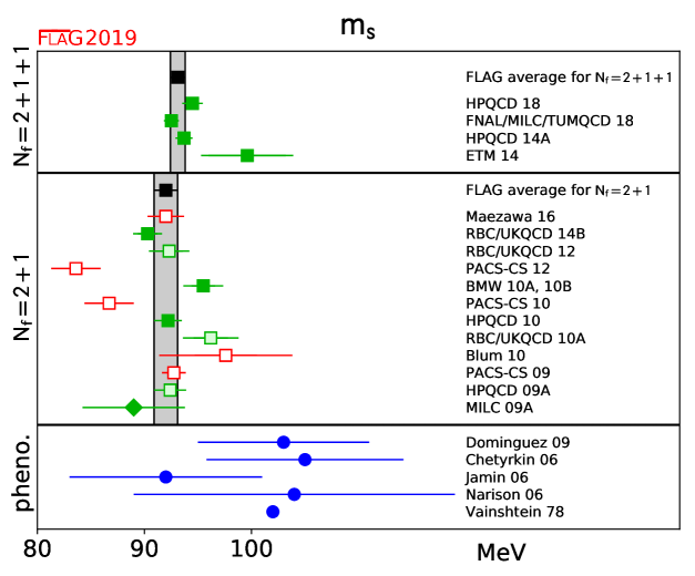
Figure 1: ${\overline{\mathrm{MS}}}$ mass of the strange quark (at 2 GeV scale) in MeV. The upper two panels show the lattice results listed in Tabs. 1 and 5, while the bottom panel collects sum rule results [Dominguez:2008jz, Chetyrkin:2005kn, Jamin:2006tj, Narison:2005ny, Vainshtein:1978nn]. Diamonds and squares represent results based on perturbative and nonperturbative renormalization, respectively. The black squares and the grey bands represent our estimates (1) and (1). The significance of the colours is explained in Sec. 2.

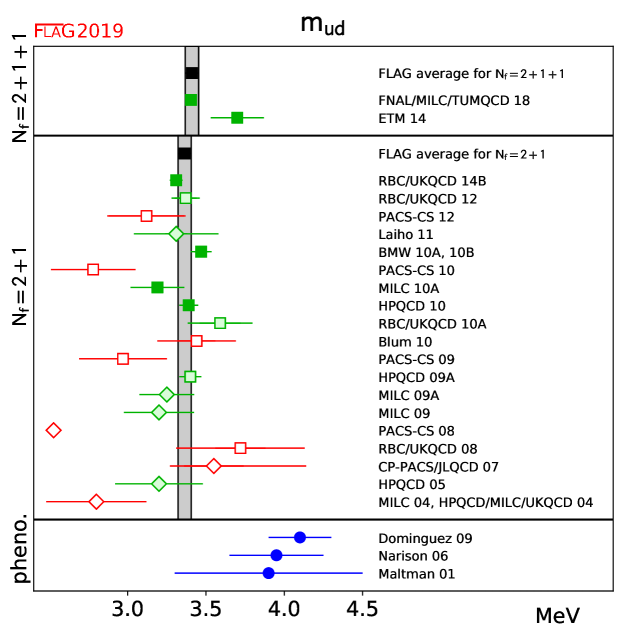
Figure 2: Mean mass of the two lightest quarks, $m_{ud}=\frac{1}{2}(m_{u}+m_{d})$. The bottom panel shows results based on sum rules [Dominguez:2008jz, Narison:2005ny, Maltman:2001nx] (for more details see Fig. 1).

3.1.5 Lattice determinations of $m_{s}/m_{ud}$

• The calculation includes electromagnetic effects.
  

• The errors are statistical, chiral and finite volume.
  

• The calculation includes electromagnetic and $m_{u}\neq m_{d}$ effects through reweighting.
  

• The fermion action used is tree-level improved.
  

• The calculation includes quenched electromagnetic effects.

Table 6: Lattice results for the ratio $m_{s}/m_{ud}$.

The lattice results for $m_{s}/m_{ud}$ are summarized in Tab. 1. In the ratio $m_{s}/m_{ud}$, one of the sources of systematic error—the uncertainties in the renormalization factors—drops out.

$N_{f}=2+1$ lattice calculations

For $N_{f}=2+1$ our average has not changed since the last version of the review and is based on the result RBC/UKQCD 14B, which replaces RBC/UKQCD 12 (see Sec. 3.1.4), and on the results MILC 09A and BMW 10A, 10B. The value quoted by HPQCD 10 does not represent independent information as it relies on the result for $m_{s}/m_{ud}$ obtained by the MILC collaboration. Averaging these results according to the prescriptions of Sec. 2.3 gives $m_{s}/m_{ud}=27.42(12)$ with $\chi^{2}/\mbox{dof}\simeq 0.2$. Since the errors associated with renormalization drop out in the ratio, the uncertainties are even smaller than in the case of the quark masses themselves: the above number for $m_{s}/m_{ud}$ amounts to an accuracy of 0.5%.

At this level of precision, the uncertainties in the electromagnetic and strong isospin-breaking corrections might not be completely negligible. Nevertheless, we decide not to add any uncertainty associated with this effect. The main reason is that most recent determinations try to estimate this uncertainty themselves and found an effect smaller than naive power counting estimates (see $N_{f}=2+1+1$ section).

$$\mbox{$N_{f}=2+1$ :}\qquad{m_{s}}/{m_{ud}}=27.42~{}(12)\qquad\,\mathrm{Refs.}~{}\mbox{\cite[cite]{[\@@bibref{Number}{Blum:2014tka,Bazavov:2009fk,Durr:2010vn,Durr:2010aw}{}{}]}}\,.$$ (37)

$N_{f}=2+1+1$ lattice calculations

For $N_{f}=2+1+1$ there are three results, MILC 17 [Bazavov:2017lyh], ETM 14 [Carrasco:2014cwa] and FNAL/MILC 14A [Bazavov:2014wgs], all of which satisfy our selection criteria.

MILC 17 uses 24 HISQ staggered-fermion ensembles at six values of the lattice spacing in the range $0.15\,{\rm fm}$–$0.03\,{\rm fm}$.

ETM 14 uses 15 twisted mass gauge ensembles at three lattice spacings ranging from 0.062 to 0.089 fm (using $f_{\pi}$ as input), in boxes of size ranging from 2.0 to 3.0 fm, and pion masses from 210 to 440 MeV (explaining the tag $\circ$ in the chiral extrapolation and the tag $\bigstar$ for the continuum extrapolation). The value of $M_{\pi}L$ at their smallest pion mass is 3.2 with more than two volumes (explaining the tag $\circ$ in the finite-volume effects). They fix the strange mass with the kaon mass.

FNAL/MILC 14A employs HISQ staggered fermions. Their result is based on 21 ensembles at four values of the coupling $\beta$ corresponding to lattice spacings in the range from 0.057 to 0.153 fm, in boxes of sizes up to 5.8 fm, and with taste-Goldstone pion masses down to 130 MeV, and RMS pion masses down to 143 MeV. They fix the strange mass with $M_{\bar{s}s}$, corrected for electromagnetic effects with $\epsilon=0.84(20)$ [Basak:2014vca]. All of our selection criteria are satisfied with the tag $\bigstar$ . Thus our average is given by $m_{s}/m_{ud}=27.23~{}(10)$, where the error includes a large stretching factor equal to $\sqrt{\chi^{2}/\mbox{dof}}\simeq 1.6$, coming from our rules for the averages discussed in Sec. 2.2. As mentioned already this is mainly due to ETM 14(A) values lying significantly above the averages for the individual masses.

$$\mbox{$N_{f}=2+1+1$ :}\qquad m_{s}/m_{ud}=27.23~{}(10)\qquad\,\mathrm{Refs.}~{}\mbox{\cite[cite]{[\@@bibref{Number}{Bazavov:2017lyh,Carrasco:2014cwa,Bazavov:2014wgs}{}{}]}},$$ (38)

which corresponds to an overall uncertainty equal to 0.4%. It is worth noting that [Bazavov:2017lyh] estimates the EM effects in this quantity to be $\sim 0.18\%$.

All the lattice results listed in Tab. 1 as well as the FLAG averages for each value of $N_{f}$ are reported in Fig. 3 and compared with $\chi$PT and sum rules.

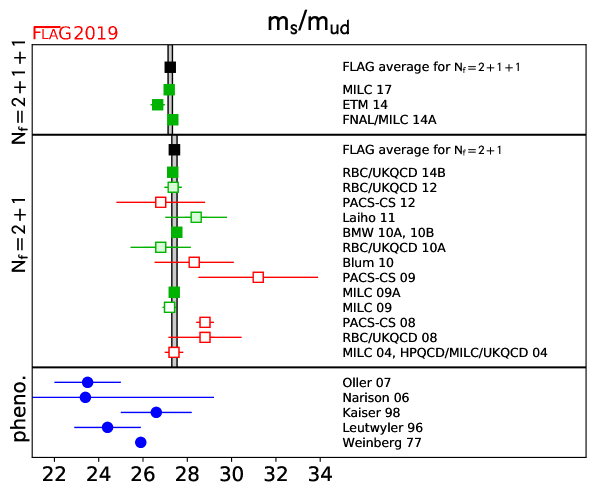
Figure 3: Results for the ratio $m_{s}/m_{ud}$. The upper part indicates the lattice results listed in Tab. 1 together with the FLAG averages for each value of $N_{f}$. The lower part shows results obtained from $\chi$PT and sum rules [Oller:2006xb, Narison:2005ny, Kaiser, Leutwyler:1996qg, Weinberg:1977hb].

3.1.6 Lattice determination of $m_{u}$ and $m_{d}$

In addition to reviewing computations of individual $m_{u}$ and $m_{d}$ quark masses, we will also determine FLAG averages for the parameter $\epsilon$ related to the violations of Dashen’s theorem

$$\epsilon=\frac{(\Delta M_{K}^{2}-\Delta M_{\pi}^{2})^{\gamma}}{\Delta M_{\pi}^{2}}\,,$$ (39)

where $\Delta M_{\pi}^{2}=M_{\pi^{+}}^{2}-M_{\pi^{0}}^{2}$ and $\Delta M_{K}^{2}=M_{K^{+}}^{2}-M_{K^{0}}^{2}$ are the pion and kaon squared mass splittings, respectively. The superscript $\gamma$, here and in the following, denotes corrections that arise from electromagnetic effects only. This parameter is often a crucial intermediate quantity in the extraction of the individual light-quark masses. Indeed, it can be shown using the $G$-parity symmetry of the pion triplet that $\Delta M_{\pi}^{2}$ does not receive $O(\delta m)$ isospin-breaking corrections. In other words

$$\Delta M_{\pi}^{2}=(\Delta M_{\pi}^{2})^{\gamma}\qquad\text{and}\qquad\epsilon=\frac{(\Delta M_{K}^{2})^{\gamma}}{\Delta M_{\pi}^{2}}-1\,,$$ (40)

at leading-order in the isospin-breaking expansion. The difference $(\Delta M_{\pi}^{2})^{SU(2)}$ was estimated in previous editions of FLAG through the $\epsilon_{m}$ parameter. However, consistent with our leading-order truncation of the isospin-breaking expansion, it is simpler to ignore this term. Once known, $\epsilon$ allows one to consistently subtract the electromagnetic part of the kaon splitting to obtain the QCD splitting $(\Delta M_{K}^{2})^{SU(2)}$. In contrast with the pion, the kaon QCD splitting is sensitive to $\delta m$, and, in particular, proportional to it at leading order in $\chi$PT. Therefore, the knowledge of $\epsilon$ allows for the determination of $\delta m$ from a chiral fit to lattice-QCD data. Originally introduced in another form in [Dashen:1969eg], $\epsilon$ vanishes in the $SU(3)$ chiral limit, a result known as Dashen’s theorem. However, in the 1990’s numerous phenomenological papers pointed out that $\epsilon$ might be an $O(1)$ number, indicating a significant failure of $SU(3)$ $\chi$PT in the description of electromagnetic effects on light meson masses. However, the phenomenological determinations of $\epsilon$ feature some level of controversy, leading to the rather imprecise estimate $\epsilon=0.7(5)$ given in the first edition of FLAG. In this edition of the review, we quote below more precise averages for $\epsilon$, directly obtained from lattice-QCD+QED simulations. We refer the reader to the previous editions of FLAG, and to the review [Portelli:2015gda] for discusions of the phenomenological determinations of $\epsilon$.

Regarding finite-volume effects for calculations including QED, this edition of FLAG uses a new quality criterion presented in Sec. 2.1.1. Indeed, due to the long-distance nature of the electromagnetic interaction, these effects are dominated by a power law in the lattice spatial size. The coefficients of this expansion depend on the chosen finite-volume formulation of QED. For $\mathrm{QED}_{\mathrm{L}}$, these effects on the squared mass $M^{2}$ of a charged meson are given by [Borsanyi:2014jba, Davoudi:2014qua, Davoudi:2018qpl]

$$\Delta_{\mathrm{FV}}M^{2}=\alpha M^{2}\left\{\frac{c_{1}}{ML}+\frac{2c_{1}}{(ML)^{2}}+\mathcal{O}\left[\frac{1}{(ML)^{3}}\right]\right\}\,,$$ (41)

with $c_{1}\simeq-2.83730$. It has been shown in [Borsanyi:2014jba] that the two first orders in this expansion are exactly known for hadrons, and are equal to the pointlike case. However, the $\mathcal{O}[1/(ML)^{3}]$ term and higher orders depend on the structure of the hadron. The universal corrections for $\mathrm{QED}_{\mathrm{TL}}$ can also be found in [Borsanyi:2014jba]. In all this part, for all computations using such universal formulae, the QED finite-volume quality criterion has been applied with $n_{\mathrm{min}}=3$, otherwise $n_{\mathrm{min}}=1$ was used.

Since FLAG 16, six new results have been reported for nondegenerate light-quark masses. In the $N_{f}=2+1+1$ sector, MILC 18 [Basak:2018yzz] computed $\epsilon$ using $N_{f}=2+1$ asqtad electro-quenched QCD+$\mathrm{QED}_{\mathrm{TL}}$ simulations and extracted the ratio $m_{u}/m_{d}$ from a new set of $N_{f}=2+1+1$ HISQ QCD simulations. Although $\epsilon$ comes from $N_{f}=2+1$ simulations, $(\Delta M_{K}^{2})^{SU(2)}$, which is about three times larger than $(\Delta M_{K}^{2})^{\gamma}$, has been determined in the $N_{f}=2+1+1$ theory. We therefore chose to classify this result as a four-flavour one. This result is explicitly described by the authors as an update of MILC 17 [Bazavov:2017lyh]. In MILC 17 [Bazavov:2017lyh], $m_{u}/m_{d}$ is determined as a side-product of a global analysis of heavy-meson decay constants, using a preliminary version of $\epsilon$ from MILC 18 [Basak:2018yzz]. In FNAL/MILC/TUMQCD 18 [Bazavov:2018omf] the ratio $m_{u}/m_{d}$ from MILC 17 [Bazavov:2017lyh] is used to determine the individual masses $m_{u}$ and $m_{d}$ from a new calculation of $m_{ud}$. The work RM123 17 [Giusti:2017dmp] is the continuation the $N_{f}=2$ result named RM123 13 [deDivitiis:2013xla] in the previous edition of FLAG. This group now uses $N_{f}=2+1+1$ ensembles from ETM 10 [Baron:2010bv], however still with a rather large minimum pion mass of $270~{}\mathrm{MeV}$, leading to the $\circ$ rating for chiral extrapolations. In the $N_{f}=2+1$ sector, BMW 16 [Fodor:2016bgu] reuses the data set produced from their determination of the light baryon octet mass splittings [Borsanyi:2013lga] using electro-quenched QCD+$\mathrm{QED}_{\mathrm{TL}}$ smeared clover fermion simulations. Finally, MILC 16 [Basak:2016jnn], which is a preliminary result for the value of $\epsilon$ published in MILC 18 [Basak:2018yzz], also provides a $N_{f}=2+1$ computation of the ratio $m_{u}/m_{d}$.

MILC 09A [Bazavov:2009fk] uses the mass difference between $K^{0}$ and $K^{+}$, from which they subtract electromagnetic effects using Dashen’s theorem with corrections, as discussed in the introduction of this section. The up and down sea quarks remain degenerate in their calculation, fixed to the value of $m_{ud}$ obtained from $M_{\pi^{0}}$. To determine $m_{u}/m_{d}$, BMW 10A, 10B [Durr:2010vn, Durr:2010aw] follow a slightly different strategy. They obtain this ratio from their result for $m_{s}/m_{ud}$ combined with a phenomenological determination of the isospin-breaking quark-mass ratio $Q=22.3(8)$, from $\eta\to 3\pi$ decays [Leutwyler:2009jg] (the decay $\eta\to 3\pi$ is very sensitive to QCD isospin breaking but fairly insensitive to QED isospin breaking).

• MILC 17 additionally quotes an optional 0.0032 uncertainty on $m_{u}/m_{d}$ corresponding to QED and QCD separation scheme ambiguities. Because this variation is not per se an error on the determination of $m_{u}/m_{d}$, and because it is generally not included in other results, we choose to omit it here. This result critically depends on $\epsilon$ determined in MILC 18, which is unpublished at present.

• Values obtained by combining the HPQCD 10 result for $m_{s}$ with the MILC 09 results for $m_{s}/m_{ud}$ and $m_{u}/m_{d}$.
  

• The fermion action used is tree-level improved.
  

• The masses are renormalized and run nonperturbatively up to a scale of $100\,\mathrm{Ge\kern-0.80005ptV}$ in the $N_{f}=2$ SF scheme. In this scheme, nonperturbative and NLO running for the quark masses are shown to agree well from 100 GeV all the way down to 2 GeV [DellaMorte:2005kg].
  

• The masses are renormalized and run nonperturbatively up to a scale of 4 GeV in the $N_{f}=3$ RI-MOM scheme. In this scheme, nonperturbative and N${}^{3}$LO running for the quark masses are shown to agree from 6 GeV down to 3 GeV to better than 1% [Durr:2010aw].

Table 7: Lattice results for $m_{u}$, $m_{d}$ (MeV) and for the ratio $m_{u}/m_{d}$. The values refer to the ${\overline{\mathrm{MS}}}$ scheme at scale 2 GeV. The top part of the table lists the result obtained with $N_{f}=2+1+1$, while the lower part presents calculations with $N_{f}=2+1$.

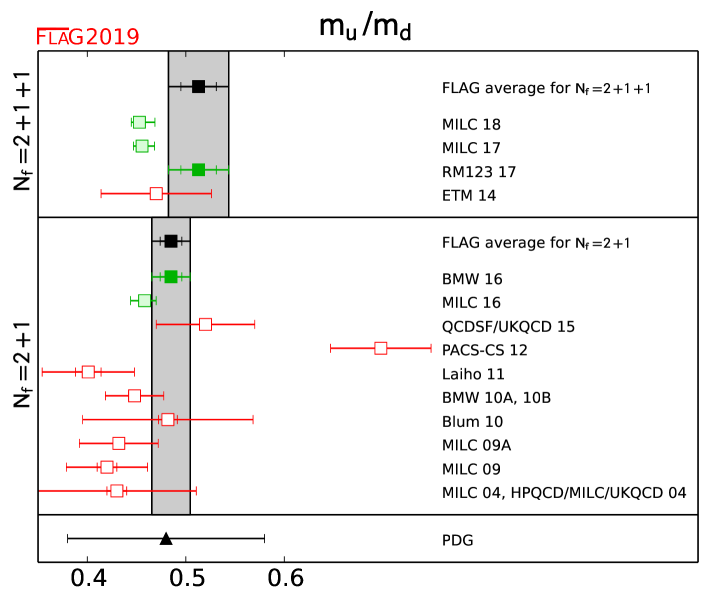
Figure 4: Lattice results and FLAG averages at $N_{f}=2+1$ and $2+1+1$ for the up-down quark masses ratio $m_{u}/m_{d}$, together with the current PDG estimate.

Instead of subtracting electromagnetic effects using phenomenology, RBC 07 [Blum:2007cy] and Blum 10 [Blum:2010ym] actually include a quenched electromagnetic field in their calculation. This means that their results include corrections to Dashen’s theorem, albeit only in the presence of quenched electromagnetism. Since the up and down quarks in the sea are treated as degenerate, very small isospin corrections are neglected, as in MILC’s calculation. PACS-CS 12 [Aoki:2012st] takes the inclusion of isospin-breaking effects one step further. Using reweighting techniques, it also includes electromagnetic and $m_{u}-m_{d}$ effects in the sea. However, they do not correct for the large finite-volume effects coming from electromagnetism in their $M_{\pi}L\sim 2$ simulations, but provide rough estimates for their size, based on Ref. [Hayakawa:2008an]. QCDSF/UKQCD 15 [Horsley:2015eaa] uses QCD+QED dynamical simulations performed at the $SU(3)$-flavour-symmetric point, but at a single lattice spacing, so they do not enter our average. The smallest partially quenched ($m_{\rm sea}\neq m_{\rm val}$) pion mass is greater than 200 MeV, so our chiral-extrapolation criteria require a $\circ$ rating. Concerning finite-volume effects, this work uses three spatial extents $L$ of $1.6~{}\mathrm{fm}$, $2.2~{}\mathrm{fm}$, and $3.3~{}\mathrm{fm}$. QCDSF/UKQCD 15 claims that the volume dependence is not visible on the two largest volumes, leading them to assume that finite-size effects are under control. As a consequence of that, the final result for quark masses does not feature a finite-volume extrapolation or an estimation of the finite-volume uncertainty. However, in their work on the QED corrections to the hadron spectrum [Horsley:2015eaa] based on the same ensembles, a volume study shows some level of compatibility with the $\mathrm{QED}_{\mathrm{L}}$ finite-volume effects derived in [Davoudi:2014qua]. We see two issues here. Firstly, the analytical result quoted from [Davoudi:2014qua] predicts large, $O(10\%)$ finite-size effects from QED on the meson masses at the values of $M_{\pi}L$ considered in QCDSF/UKQCD 15, which is inconsistent with the statement made in the paper. Secondly, it is not known that the zero-mode regularization scheme used here has the same volume scaling as $\mathrm{QED}_{\mathrm{L}}$. We therefore chose to assign the $\blacksquare$ rating for finite volume to QCDSF/UKQCD 15. Finally, for $N_{f}=2+1+1$, ETM 14 [Carrasco:2014cwa] uses simulations in pure QCD, but determines $m_{u}-m_{d}$ from the slope $\partial M_{K}^{2}/\partial m_{ud}$ and the physical value for the QCD kaon-mass splitting taken from the phenomenological estimate in FLAG 13.

Lattice results for $m_{u}$, $m_{d}$ and $m_{u}/m_{d}$ are summarized in Tab. 1. It is important to notice two major changes in the grading of these results: the introduction of an “isospin breaking” criterion and the modification of the “finite volume” criterion in the presence of QED. The colour coding is specified in detail in Sec. 2.1. Considering the important progress in the last years on including isospin-breaking effects in lattice simulations, we are now in a position where averages for $m_{u}$ and $m_{d}$ can be made without the need of phenomenological inputs. Therefore, lattice calculations of the individual quark masses using phenomenological inputs for isospin-breaking effects will be coded $\blacksquare$.

We start by recalling the $N_{f}=2$ FLAG estimate for the light-quark masses, entirely coming from RM123 13 [deDivitiis:2013xla],

$$m_{u} =2.40(23)\,\mathrm{Me\kern-1.00006ptV} \ref{~}\mbox{\cite[cite]{[\@@bibref{Number}{deDivitiis:2013xla}{}{}]}}\,,$$

$$N_{f}=2:\hskip 5.69046pt m_{d} =4.80(23)\,\mathrm{Me\kern-1.00006ptV} \ref{~}\mbox{\cite[cite]{[\@@bibref{Number}{deDivitiis:2013xla}{}{}]}}\,,$$ (42)

$${m_{u}}/{m_{d}} =0.50(4) \ref{~}\mbox{\cite[cite]{[\@@bibref{Number}{deDivitiis:2013xla}{}{}]}}\,,$$

with errors of roughly 10%, 5% and 8%, respectively. In these results, the errors are obtained by combining the lattice statistical and systematic errors in quadrature. For $N_{f}=2+1$, the only result, which qualifies for entering the FLAG average for quark masses, is BMW 16 [Fodor:2016bgu],

$$m_{u} =2.27(9)\,\mathrm{Me\kern-1.00006ptV} \ref{~}\mbox{\cite[cite]{[\@@bibref{Number}{Fodor:2016bgu}{}{}]}}\,,$$

$$N_{f}=2+1:\hskip 5.69046pt m_{d} =4.67(9)\,\mathrm{Me\kern-1.00006ptV} \ref{~}\mbox{\cite[cite]{[\@@bibref{Number}{Fodor:2016bgu}{}{}]}}\,,$$ (43)

$${m_{u}}/{m_{d}} =0.485(19) \ref{~}\mbox{\cite[cite]{[\@@bibref{Number}{Fodor:2016bgu}{}{}]}}\,,$$

with errors of roughly 4%, 2% and 4%, respectively. This estimate is slightly more precise than in the previous edition of FLAG. More importantly, it now comes entirely from a lattice-QCD+QED calculation, whereas phenomenological input was used in previous editions. These numbers result in the following RGI averages

$$M_{u}^{\rm RGI} =3.16(13)_{m}(4)_{\Lambda}\,\mathrm{Me\kern-1.00006ptV}=3.16(13)\,\mathrm{Me\kern-1.00006ptV} \ref{~}\mbox{\cite[cite]{[\@@bibref{Number}{Fodor:2016bgu}{}{}]}}\,,$$

$$N_{f}=2+1:\hskip 5.69046pt$$ (44)

$$M_{d}^{\rm RGI} =6.50(13)_{m}(8)_{\Lambda}\,\mathrm{Me\kern-1.00006ptV}=6.50(15)\,\mathrm{Me\kern-1.00006ptV} \ref{~}\mbox{\cite[cite]{[\@@bibref{Number}{Fodor:2016bgu}{}{}]}}\,.$$

Finally, for $N_{f}=2+1+1$, only RM123 17 [Giusti:2017dmp] enters the average, giving

$$m_{u} =2.50(17)\,\mathrm{Me\kern-1.00006ptV} \ref{~}\mbox{\cite[cite]{[\@@bibref{Number}{Giusti:2017dmp}{}{}]}}\,,$$

$$N_{f}=2+1+1:\hskip 4.26773pt m_{d} =4.88(20)\,\mathrm{Me\kern-1.00006ptV} \ref{~}\mbox{\cite[cite]{[\@@bibref{Number}{Giusti:2017dmp}{}{}]}}\,,$$ (45)

$${m_{u}}/{m_{d}} =0.513(31) \ref{~}\mbox{\cite[cite]{[\@@bibref{Number}{Giusti:2017dmp}{}{}]}}\,.$$

with errors of roughly 7%, 4% and 6%, respectively. In the previous edition of FLAG, ETM 14 [Carrasco:2014cwa] was used for the average. The RM123 17 result used here is slightly more precise and is free of phenomenological input. The value of $m_{u}/m_{d}$ in MILC 17 [Bazavov:2017lyh] depends critically on the value of $\epsilon$ given in MILC 18 [Basak:2018yzz], which was unpublished at the time of the review deadline. As a consequence we did not include the result MILC 17 [Bazavov:2017lyh] in the average. The value will appear in the average of the online version of the review. It is, however important to point out that both MILC 17 and MILC 18 results show a marginal discrepancy with RM123 17 [Giusti:2017dmp] of $1.7$ standard deviations. The RGI averages are

$$M_{u}^{\rm RGI} =3.48(24)_{m}(4)_{\Lambda}\,\mathrm{Me\kern-1.00006ptV}=3.48(24)\,\mathrm{Me\kern-1.00006ptV} \ref{~}\mbox{\cite[cite]{[\@@bibref{Number}{Giusti:2017dmp}{}{}]}}\,,$$

$$N_{f}=2+1+1:\hskip 4.26773pt$$ (46)

$$M_{d}^{\rm RGI} =6.80(28)_{m}(8)_{\Lambda}\,\mathrm{Me\kern-1.00006ptV}=6.80(29)\,\mathrm{Me\kern-1.00006ptV} \ref{~}\mbox{\cite[cite]{[\@@bibref{Number}{Giusti:2017dmp}{}{}]}}\,.$$

Every result for $m_{u}$ and $m_{d}$ used here to produce the FLAG averages relies on electro-quenched calculations, so there is some interest to comment on the size of quenching effects. Considering phenomenology and the lattice results presented here, it is reasonable for a rough estimate to use the value $(\Delta M_{K}^{2})^{\gamma}\sim 2000~{}\mathrm{MeV}^{2}$ for the QED part of the kaon splitting. Using the arguments presented in Sec. 3.1.3, one can assume that the QED sea contribution represents $O(10\%)$ of $(\Delta M_{K}^{2})^{\gamma}$. Using $SU(3)$ PQ$\chi$PT+QED [Bijnens:2006mk, Portelli:2012pn] gives a $\sim 5\%$ effect. Keeping the more conservative $10\%$ estimate and using the experimental value of the kaon splitting, one finds that the QCD kaon splitting $(\Delta M_{K}^{2})^{SU(2)}$ suffers from a reduced $3\%$ quenching uncertainty. Considering that this splitting is proportional to $m_{u}-m_{d}$ at leading order in $SU(3)$ $\chi$PT, we can estimate that a similar error will propagate to the quark masses. So the individual up and down masses look mildly affected by QED quenching. However, one notices that $\sim 3\%$ is the level of error in the new FLAG averages, and increasing significantly this accuracy will require using fully unquenched calculations.

In view of the fact that a massless up-quark would solve the strong CP-problem, many authors have considered this an attractive possibility, but the results presented above exclude this possibility: the value of $m_{u}$ in Eq. (43) differs from zero by $25$ standard deviations. We conclude that nature solves the strong CP-problem differently.

Finally, we conclude this section by giving the FLAG averages for $\epsilon$ defined in Eq. (39). For $N_{f}=2+1+1$, we average the RM123 17 [Giusti:2017dmp] result with the value of $(\Delta M_{K}^{2})^{\gamma}$ from BMW 14 [Borsanyi:2014jba] combined with Eq. (40), giving

$$\epsilon=0.79(7)\,.$$ (47)

Although BMW 14 [Borsanyi:2014jba] focuses on hadron masses and did not extract the light-quark masses, they are the only fully unquenched QCD+QED calculation to date that qualifies to enter a FLAG average. With the exception of renormalization which is not discussed in the paper, this work has a $\bigstar$ rating for every FLAG criterion considered for the $m_{u}$ and $m_{d}$ quark masses. For $N_{f}=2+1$ we use the results from BMW 16 [Fodor:2016bgu]

$$\epsilon=0.73(17)\,.$$ (48)

These results are entirely determined from lattice-QCD+QED and represent an improvement of the error by a factor of two to three on the FLAG 16 phenomenological estimate.

It is important to notice that the $\epsilon$ uncertainties from BMW 16 and RM123 17 are dominated by estimates of the QED quenching effects. Indeed, in contrast with the quark masses, $\epsilon$ is expected to be rather sensitive to the sea quark-QED constributions. Using the arguments presented in Sec. 3.1.3, if one conservatively assumes that the QED sea contributions represent $O(10\%)$ of $(\Delta M_{K}^{2})^{\gamma}$, then Eq. (40) implies that $\epsilon$ will have a quenching error of $\sim 0.15$ for $(\Delta M_{K}^{2})^{\gamma}\sim 2000~{}\mathrm{MeV}^{2}$, representing a large $\sim 20\%$ relative error. It is interesting to observe that such a discrepancy does not appear between BMW 15 and RM123 17, although the $\sim 10\%$ accuracy of both results might not be sufficient to resolve these effects. To conclude, although the controversy around the value of $\epsilon$ has been significantly reduced by lattice-QCD+QED determinations, computing this quantity precisely requires fully unquenched simulations.

3.1.7 Estimates for $R$ and $Q$

The quark-mass ratios

$$R\equiv\frac{m_{s}-m_{ud}}{m_{d}-m_{u}}\hskip 14.22636pt\mbox{and}\hskip 14.22636ptQ^{2}\equiv\frac{m_{s}^{2}-m_{ud}^{2}}{m_{d}^{2}-m_{u}^{2}}$$ (49)

compare $SU(3)$ breaking with isospin breaking. Both numbers only depend on the ratios $m_{s}/m_{ud}$ and $m_{u}/m_{d}$,

$$R=\frac{1}{2}\left(\frac{m_{s}}{m_{ud}}-1\right)\frac{1+\frac{m_{u}}{m_{d}}}{1-\frac{m_{u}}{m_{d}}}\qquad\text{and}\qquad Q^{2}=\frac{1}{2}\left(\frac{m_{s}}{m_{ud}}+1\right)R\,.$$ (50)

The quantity $Q$ is of particular interest because of a low-energy theorem [Gasser:1984pr], which relates it to a ratio of meson masses,

$$Q^{2}_{M}\equiv\frac{\hat{M}_{K}^{2}}{\hat{M}_{\pi}^{2}}\frac{\hat{M}_{K}^{2}-\hat{M}_{\pi}^{2}}{\hat{M}_{K^{0}}^{2}-\hat{M}_{K^{+}}^{2}}\,,\hskip 28.45274pt\hat{M}^{2}_{\pi}\equiv\mbox{$\frac{1}{2}$}(\hat{M}^{2}_{\pi^{+}}+\hat{M}^{2}_{\pi^{0}})\,,\hskip 14.22636pt\hat{M}^{2}_{K}\equiv\mbox{$\frac{1}{2}$}(\hat{M}^{2}_{K^{+}}+\hat{M}^{2}_{K^{0}})\,.$$ (51)

Chiral symmetry implies that the expansion of $Q_{M}^{2}$ in powers of the quark masses (i) starts with $Q^{2}$ and (ii) does not receive any contributions at NLO:

$$Q_{M}\stackrel{{\scriptstyle\rule[-2.84544pt]{0.0pt}{0.0pt}\mbox{\tiny NLO}}}{{=}}Q\,.$$ (52)

We recall here the $N_{f}=2$ estimates for $Q$ and $R$ from FLAG 16,

$$R=40.7(3.7)(2.2)\,,\hskip 56.9055ptQ=24.3(1.4)(0.6)\ ,$$ (53)

where the second error comes from the phenomenological inputs that were used. For $N_{f}=2+1$, we use Eqs. (37) and (43) and obtain

$$R=38.1(1.5)\,,\hskip 56.9055ptQ=23.3(0.5)\ ,$$ (54)

where now only lattice results have been used. For $N_{f}=2+1+1$ we obtain

$$R=40.7(2.7)\,,\hskip 56.9055ptQ=24.0(0.8)\ ,$$ (55)

which are quite compatible with two- and three-flavour results. It is interesting to notice that the most recent phenomenological determination of $R$ and $Q$ from $\eta\to 3\pi$ decay [Colangelo:2018jxw] gives the values $R=34.4(2.1)$ and $Q=22.1(7)$, which are marginally discrepant with the averages presented here. For $N_{f}=2+1$, the discrepancy is $1.4$ standard deviations for both $R$ and $Q$. For $N_{f}=2+1+1$ it is $1.8$ standard deviations. The authors of [Colangelo:2018jxw] point out that this discrepancy is due to surprisingly large corrections to the approximation (52) used in the phenomenological analysis.

Our final results for the masses $m_{u}$, $m_{d}$, $m_{ud}$, $m_{s}$ and the mass ratios $m_{u}/m_{d}$, $m_{s}/m_{ud}$, $R$, $Q$ are collected in Tabs. 8 and 9. We separate $m_{u}$, $m_{d}$, $m_{u}/m_{d}$, $R$ and $Q$ from $m_{ud}$, $m_{s}$ and $m_{s}/m_{ud}$, because the latter are completely dominated by lattice results while the former still include some phenomenological input.

$N_{f}$	$m_{ud}$	$m_{s}$	$m_{s}/m_{ud}$
2+1+1	3.410(43)	93.44(68)	27.23(10)
2+1	3.364(41)	92.03(88)	27.42(12)

Table 8: Our estimates for the strange-quark and the average up-down-quark masses in the ${\overline{\mathrm{MS}}}$ scheme at running scale $\mu=2\,\mathrm{Ge\kern-1.00006ptV}$. Mass values are given in MeV. In the results presented here, the error is the one which we obtain by applying the averaging procedure of Sec. 2.3 to the relevant lattice results. We have added an uncertainty to the $N_{f}=2+1$ results, associated with the neglect of the charm sea-quark and isospin-breaking effects, as discussed around Eqs. (1) and (37).

$N_{f}$	$m_{u}$	$m_{d}$	$m_{u}/m_{d}$	$R$	$Q$
2+1+1	2.50(17)	4.88(20)	0.513(31)	40.7(2.7)	24.0(0.8)
2+1	2.27(9)	4.67(9)	0.485(19)	38.1(1.2)	23.3(0.5)

Table 9: Our estimates for the masses of the two lightest quarks and related, strong isospin-breaking ratios. Again, the masses refer to the ${\overline{\mathrm{MS}}}$ scheme at running scale $\mu=2\,\mathrm{Ge\kern-1.00006ptV}$. Mass values are given in MeV.

3.2 Charm quark mass

In the following, we collect and discuss the lattice determinations of the $\overline{\rm MS}$ charm-quark mass $\overline{m}_{c}$. Most of the results have been obtained by analyzing the lattice-QCD simulations of two-point heavy-light- or heavy-heavy-meson correlation functions, using as input the experimental values of the $D$, $D_{s}$, and charmonium mesons. Other groups use the moments method. The latter is based on the lattice calculation of the Euclidean time moments of pseudoscalar-pseudoscalar correlators for heavy-quark currents followed by an OPE expansion dominated by perturbative QCD effects, which provides the determination of both the heavy-quark mass and the strong-coupling constant $\alpha_{s}$.

The heavy-quark actions adopted by various lattice collaborations have been discussed in previous FLAG reviews [Aoki:2013ldr, Aoki:2016frl], and their descriptions can be found in Sec. LABEL:app:HQactions. While the charm mass determined with the moments method does not need any lattice evaluation of the mass-renormalization constant $Z_{m}$, the extraction of $\overline{m}_{c}$ from two-point heavy-meson correlators does require the nonperturbative calculation of $Z_{m}$. The lattice scale at which $Z_{m}$ is obtained, is usually at least of the order $2$–$3$ GeV, and therefore it is natural in this review to provide the values of $\overline{m}_{c}(\mu)$ at the renormalization scale $\mu=3~{}\mathrm{Ge\kern-1.00006ptV}$. Since the choice of a renormalization scale equal to $\overline{m}_{c}$ is still commonly adopted (as by PDG [Agashe:2014kda]), we have collected in Tab. 1 the lattice results for both $\overline{m}_{c}(\overline{m}_{c})$ and $\overline{m}_{c}(\mbox{3 GeV})$, obtained for $N_{f}=2+1$ and $2+1+1$. This year’s review does not contain results for $N_{f}=2$, and interested readers are referred to previous reviews [Aoki:2013ldr, Aoki:2016frl].

When not directly available in the published work, we apply a conversion factor equal either to $0.900$ between the scales $\mu=2$ GeV and $\mu=3$ GeV or to $0.766$ between the scales $\mu=\overline{m}_{c}$ and $\mu=3$ GeV, obtained using perturbative QCD evolution at four loops assuming $\Lambda_{QCD}=300$ MeV for $N_{f}=4$.

Table 10: Lattice results for the ${\overline{\mathrm{MS}}}$-charm-quark mass $\overline{m}_{c}(\overline{m}_{c})$ and $\overline{m}_{c}(\mbox{3 GeV})$ in GeV, together with the colour coding of the calculations used to obtain these. When not directly available in a publication, we employ a conversion factor equal to $0.900$ between the scales $\mu=2$ GeV and $\mu=3$ GeV (or, $0.766$ between $\mu=\overline{m}_{c}$ and $\mu=3$ GeV).

In the next subsections, we review separately the results of $\overline{m}_{c}(\overline{m}_{c})$ for the various values of $N_{f}$.

3.2.1 $N_{f}=2+1$ results

The HPQCD 10 [McNeile:2010ji] result is computed from moments, using a subset of $N_{f}=2+1$ Asqtad-staggered-fermion ensembles from MILC [Bazavov:2009bb] and HISQ valence fermions. The charm mass is fixed from the $\eta_{c}$ meson, $M_{\eta_{c}}=2.9852(34)~{}\mathrm{Ge\kern-1.00006ptV}$, corrected for $\bar{c}c$ annihilation and electromagnetic effects. HPQCD 10 supersedes the HPQCD 08B [Allison:2008xk] result using valence-Asqtad-staggered fermions.

$\chi$QCD 14 [Yang:2014sea] uses a mixed-action approach based on overlap fermions for the valence quarks and domain-wall fermions for the sea quarks. They adopt six of the gauge ensembles generated by the RBC/UKQCD collaboration [Aoki:2010dy] at two values of the lattice spacing (0.087 and 0.11 fm) with unitary pion masses in the range from 290 to 420 MeV. For the valence quarks no light-quark masses are simulated. At the lightest pion mass $M_{\pi}\simeq$ 290 MeV, $M_{\pi}L=4.1$, which satisfies the tag $\circ$ for finite-volume effects. The strange- and charm-quark masses are fixed together with the lattice scale by using the experimental values of the $D_{s}$, $D_{s}^{*}$ and $J/\psi$ meson masses.

JLQCD 15B [Nakayama:2015hrn] determines the charm mass by using the moments method and Möbius domain-wall fermions at three values of the lattice spacing, ranging from 0.044 to 0.083 fm. They employ 15 ensembles in all, including several different pion masses and volumes. The lightest pion mass is $\simeq 230$ MeV with $M_{\pi}L$ is $\simeq 4.4$. The linear size of their lattices is in the range 2.6–3.8 fm.

Since FLAG 16 there have been two new results, JLQCD 16 [Nakayama:2016atf] and Maezawa 16 [Maezawa:2016vgv]. The former supersedes JLQCD 15B as it is a published update of their previous preliminary result. The latter employs the moments method using pseudoscalar correlation functions computed with HISQ fermions on a set of 11 ensembles with lattices spacing in the range 0.04 to 0.14 fm. Only a single pion mass of 160 MeV is studied. The linear size of the lattices take on values between 2.5 and 5.2 fm.

Thus, according to our rules on the publication status, the FLAG average for the charm-quark mass at $N_{f}=2+1$ is obtained by combining the results HPQCD 10, $\chi$QCD 14, and JLQCD 16,

$$\overline{m}_{c}(\overline{m}_{c}) =1.275~{}(5)~{}\mathrm{Ge\kern-1.00006ptV} \,\mathrm{Refs.}~{}\mbox{\cite[cite]{[\@@bibref{Number}{McNeile:2010ji,Yang:2014sea,Nakayama:2016atf}{}{}]}}\,,$$ (56)

$$N_{f}=2+1$$:

$$\overline{m}_{c}(\mbox{3 GeV}) =0.992~{}(6)~{}\mathrm{Ge\kern-1.00006ptV} \,\mathrm{Refs.}~{}\mbox{\cite[cite]{[\@@bibref{Number}{McNeile:2010ji,Yang:2014sea,Nakayama:2016atf}{}{}]}}\,,$$ (57)

where the error on $\overline{m}_{c}(\mbox{3 GeV})$ includes a stretching factor $\sqrt{\chi^{2}/\mbox{dof}}\simeq 1.18$ as discussed in Sec. 2.2. This result corresponds to the following RGI average

$$M_{c}^{\rm RGI} =1.529(9)_{m}(14)_{\Lambda}~{}\mathrm{Ge\kern-1.00006ptV}=1.529(17)~{}\mathrm{Ge\kern-1.00006ptV} \,\mathrm{Refs.}~{}\mbox{\cite[cite]{[\@@bibref{Number}{McNeile:2010ji,Yang:2014sea,Nakayama:2016atf}{}{}]}}\,.$$ (58)

3.2.2 $N_{f}=2+1+1$ results

In FLAG 16 three results employing four dynamical quarks in the sea were discussed. ETM 14 [Carrasco:2014cwa] uses 15 twisted-mass gauge ensembles at three lattice spacings ranging from 0.062 to 0.089 fm, in boxes of size ranging from 2.0 to 3.0 fm and pion masses from 210 to 440 MeV (explaining the tag $\circ$ in the chiral extrapolation and the tag $\bigstar$ for the continuum extrapolation). The value of $M_{\pi}L$ at their smallest pion mass is 3.2 with more than two volumes (explaining the tag $\circ$ in the finite-volume effects). They fix the strange mass with the kaon mass and the charm one with that of the $D_{s}$ and $D$ mesons.

ETM 14A [Alexandrou:2014sha] uses 10 out of the 15 gauge ensembles adopted in ETM 14 spanning the same range of values for the pion mass and the lattice spacing, but the latter is fixed using the nucleon mass. Two lattice volumes with size larger than 2.0 fm are employed. The physical strange and the charm mass are obtained using the masses of the $\Omega^{-}$ and $\Lambda_{c}^{+}$ baryons, respectively.

HPQCD 14A [Chakraborty:2014aca] employs the moments method with HISQ fermions. Their results are based on 9 out of the 21 ensembles produced by the MILC collaboration [Bazavov:2014wgs]. Lattice spacings range from 0.057 to 0.153 fm, with box sizes up to 5.8 fm and taste-Goldstone-pion masses down to 130 MeV. The RMS-pion masses go down to 173 MeV. The strange- and charm-quark masses are fixed using $M_{\bar{s}s}=688.5(2.2)~{}\mathrm{Me\kern-1.00006ptV}$, calculated without including $\bar{s}s$ annihilation effects, and $M_{\eta_{c}}=2.9863(27)~{}\mathrm{Ge\kern-1.00006ptV}$, obtained from the experimental $\eta_{c}$ mass after correcting for $\bar{c}c$ annihilation and electromagnetic effects. All of the selection criteria of Sec. 2.1.1 are satisfied with the tag $\bigstar$.

Since FLAG 16 two groups, FNAL/MILC/TUMQCD and HPQCD have produced new values for the charm-quark mass [Bazavov:2018omf, Lytle:2018evc]. The latter use nonperturbative renormalization in the RI-SMOM scheme as described in the strange quark section and the same HISQ ensembles and valence quarks as those described in HPQCD 14A [Chakraborty:2014aca].

The FNAL/MILC/TUMQCD groups use a new minimal-renormalon-subtraction scheme (MRS) [Brambilla:2017hcq] and a sophisticated, but complex, fit strategy incorporating three effective field theories: heavy quark effective theory (HQET), heavy-meson rooted all-staggered chiral perturbation theory (HMrAS$\chi$PT), and Symanzik effective theory for cutoff effects. Heavy-light meson masses are computed from fits to lattice-QCD correlation functions. They employ HISQ quarks on 20 MILC 2+1+1 flavour ensembles with six lattice spacings between 0.03 and 0.15 fm (the largest is used only in the estimation of the systematic error in the continuum-limit extrapolation). The pion mass is physical on several ensembles except the finest, and $M_{\pi}L=3.7$–$3.9$ on the physical mass ensembles. The light-quark masses are fixed from meson masses in pure QCD, which have been shifted from their physical values using $O(\alpha)$ electromagnetic effects recently computed by the MILC collaboration [Basak:2018yzz], see Sec. 3.1.6 for details. The heavy-light mesons are shifted using a phenomenological formula. Using chiral perturbation theory at NLO and NNLO, the results are corrected for exponentially small finite-volume effects. They find that nonexponential finite-volume effects due to nonequilibration of topological charge are negligible compared to other quoted errors. These allow for a combined continuum, chiral, and infinite-volume limit from a global fit including 77 free parameters to 324 data points which satisfies all of the FLAG criteria.

All four results enter the FLAG average for $N_{f}=2+1+1$ quark flavours. We note however that while the determinations of $\overline{m}_{c}$ by ETM 14 and 14A agree well with each other, they are incompatible with HPQCD 14A, HPQCD 18, and FNAL/MILC/TUMQCD 18 by several standard deviations. While the latter use the same configurations, the analyses are quite different and independent. As mentioned earlier, $m_{ud}$ and $m_{s}$ are also systematically high compared to their respective averages. In addition, the other four-flavour values are consistent with the three-flavour average. Combining all four results yields

$$\overline{m}_{c}(\overline{m}_{c}) =1.280~{}(13)~{}\mathrm{Ge\kern-1.00006ptV} \,\mathrm{Refs.}~{}\mbox{\cite[cite]{[\@@bibref{Number}{Carrasco:2014cwa,Alexandrou:2014sha,Chakraborty:2014aca,Bazavov:2018omf,Lytle:2018evc}{}{}]}}\,,$$ (59)

$$N_{f}=2+1+1$$:

$$\overline{m}_{c}(\mbox{3 GeV}) =0.988~{}(7)~{}\mathrm{Ge\kern-1.00006ptV} \,\mathrm{Refs.}~{}\mbox{\cite[cite]{[\@@bibref{Number}{Carrasco:2014cwa,Chakraborty:2014aca,Alexandrou:2014sha,Bazavov:2018omf,Lytle:2018evc}{}{}]}}\,,$$ (60)

where the errors include large stretching factors $\sqrt{\chi^{2}/\mbox{dof}}\approx 2.0$ and $1.7$, respectively. We have assumed 100% correlation for statistical errors between ETM results. For HPQCD 14A, HPQCD 18, and FNAL/MILC/TUMQCD 18 we use the correlations given in Ref. [Lytle:2018evc]. Our fits have $\chi^{2}/\mbox{dof}=3.9$ and 2.8, respectively. The RGI average reads as follows

$$M_{c}^{\rm RGI} =1.523(11)_{m}(14)_{\Lambda}~{}\mathrm{Ge\kern-1.00006ptV}=1.523(18)~{}\mathrm{Ge\kern-1.00006ptV} \,\mathrm{Refs.}~{}\mbox{\cite[cite]{[\@@bibref{Number}{Carrasco:2014cwa,Chakraborty:2014aca,Alexandrou:2014sha,Bazavov:2018omf,Lytle:2018evc}{}{}]}}\,.$$ (61)

Figure 5 presents the results given in Tab. 1 along with the FLAG averages obtained for $2+1$ and $2+1+1$ flavours.

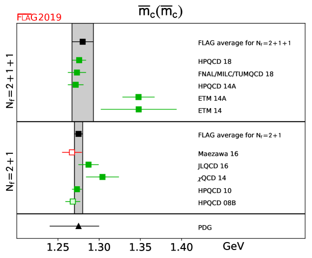
Figure 5: The charm quark mass for $2+1$ and $2+1+1$ flavours. For the latter a large stretching factor is used for the FLAG average due to poor $\chi^{2}$ from our fit.

3.2.3 Lattice determinations of the ratio $m_{c}/m_{s}$

Because some of the results for the light-quark masses given in this review are obtained via the quark-mass ratio $m_{c}/m_{s}$, we review these lattice calculations, which are listed in Tab. 11.

Collaboration	Ref.	$N_{f}$	publication status	chiral extrapolation	continuum extrapolation	finite volume	$m_{c}/m_{s}$
FNAL/MILC/TUMQCD 18	[Bazavov:2018omf]	2+1+1	A	$\bigstar$	$\bigstar$	$\bigstar$	11.784(11)(17)(00)(08)
HPQCD 14A	[Chakraborty:2014aca]	2+1+1	A	$\bigstar$	$\bigstar$	$\bigstar$	11.652(35)(55)
FNAL/MILC 14A	[Bazavov:2014wgs]	2+1+1	A	$\bigstar$	$\bigstar$	$\bigstar$	11.747(19)(${}^{+59}_{-43}$)
ETM 14	[Carrasco:2014cwa]	2+1+1	A	$\circ$	$\bigstar$	$\circ$	11.62(16)
Maezawa 16	[Maezawa:2016vgv]	2+1	A	$\blacksquare$	$\bigstar$	$\bigstar$	11.877(91)
$\chi$QCD 14	[Yang:2014sea]	2+1	A	$\circ$	$\circ$	$\circ$	11.1(8)
HPQCD 09A	[Davies:2009ih]	2+1	A	$\circ$	$\bigstar$	$\bigstar$	11.85(16)

Table 11: Lattice results for the quark-mass ratio $m_{c}/m_{s}$, together with the colour coding of the calculations used to obtain these.

The $N_{f}=2+1$ results from $\chi$QCD 14 and HPQCD 09A [Davies:2009ih] are the same as described for the charm-quark mass, and in addition the latter fixes the strange mass using $M_{\bar{s}s}=685.8(4.0)\,\mathrm{Me\kern-1.00006ptV}$. Since FLAG 16 another result has appeared, Maezawa 16 which does not pass our chiral-limit test (as described in the previous section), though we note that it is quite consistent with the other values. Combining $\chi$QCD 14 and HPQCD 09A, we obtain the same result reported in FLAG 16,

$$\mbox{$N_{f}=2+1$:}\qquad m_{c}/m_{s}=11.82~{}(16)\qquad\,\mathrm{Refs.}~{}\mbox{\cite[cite]{[\@@bibref{Number}{Yang:2014sea,Davies:2009ih}{}{}]}},$$ (62)

with a $\chi^{2}/\mbox{dof}\simeq 0.85$.

Turning to $N_{f}=2+1+1$, in addition to the HPQCD 14A and ETM 14 calculations, already described in Sec. 3.2.2, we consider the recent FNAL/MILC/TUMQCD 18 value [Bazavov:2018omf] (which updates and replaces [Bazavov:2014wgs]), where HISQ fermions are employed as described in the previous section. As for the HPQCD 14A result, all of our selection criteria are satisfied with the tag $\bigstar$. However, some tension exists between the HPQCD and FNAL/MILC/TUMQCD results. Combining all three yields

$$\mbox{$N_{f}=2+1+1$:}\qquad m_{c}/m_{s}=11.768~{}(33)\qquad\,\mathrm{Refs.}~{}\mbox{\cite[cite]{[\@@bibref{Number}{Chakraborty:2014aca,Carrasco:2014cwa,Bazavov:2018omf}{}{}]}},$$ (63)

where the error includes the stretching factor $\sqrt{\chi^{2}/\mbox{dof}}\simeq 1.5$, and $\chi^{2}/dof=2.28$. We have assumed a 100% correlation of statistical errors for FNAL/MILC/TUMQCD 18 and HPQCD 14A.

Results for $m_{c}/m_{s}$ are shown in Fig. 6 together with the FLAG averages for $2+1$ and $2+1+1$ flavours.

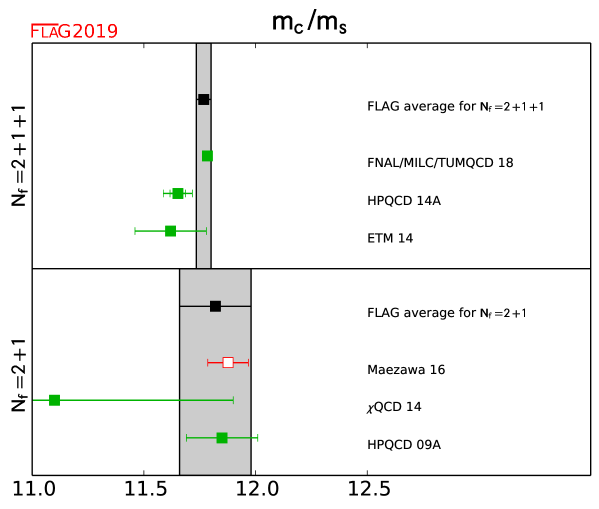
Figure 6: Lattice results for the ratio $m_{c}/m_{s}$ listed in Tab. 11 and the FLAG averages corresponding to $2+1$ and $2+1+1$ quark flavours. The latter average includes a large stretching factor on the error due a poor $\chi^{2}$ from our fit.

3.3 Bottom-quark mass

Now we review the lattice results for the $\overline{\rm MS}$-bottom-quark mass $\overline{m}_{b}$. Related heavy-quark actions and observables have been discussed in the FLAG 13 and 17 reviews [Aoki:2013ldr, Aoki:2016frl], and descriptions can be found in Sec. LABEL:app:HQactions. In Tab. 1 we collect results for $\overline{m}_{b}(\overline{m}_{b})$ obtained with $N_{f}=2+1$ and $2+1+1$ quark flavours in the sea. Available results for the quark-mass ratio $m_{b}/m_{c}$ are also reported. After discussing the various results we evaluate the corresponding FLAG averages.

• The lattice spacing used in ETM 14B has been updated here.
  

• Only two pion points are used for chiral extrapolation.
  

• The number that is given is $m_{b}(10~{}\mathrm{Ge\kern-0.80005ptV},N_{f}=5)=3.617(25)~{}\mathrm{Ge\kern-0.80005ptV}$.

Table 12: Lattice results for the ${\overline{\mathrm{MS}}}$-bottom-quark mass $\overline{m}_{b}(\overline{m}_{b})$ in GeV, together with the systematic error ratings for each. Available results for the quark mass ratio $m_{b}/m_{c}$ are also reported.

3.3.1 $N_{f}=2+1$

HPQCD 13B  [Lee:2013mla] extracts $\overline{m}_{b}$ from a lattice determination of the $\Upsilon$ energy in NRQCD and the experimental value of the meson mass. The latter quantities yield the pole mass which is related to the $\overline{\rm MS}$ mass in 3-loop perturbation theory. The MILC coarse (0.12 fm) and fine (0.09 fm) Asqtad-2+1-flavour ensembles are employed in the calculation. The bare light-(sea)-quark masses correspond to a single, relatively heavy, pion mass of about 300 MeV. No estimate of the finite-volume error is given. This result is not used in our average.

The value of $\overline{m}_{b}(\overline{m}_{b})$ reported in HPQCD 10 [McNeile:2010ji] is computed in a very similar fashion to the one in HPQCD 14A described in the following section on 2+1+1 flavour results, except that MILC 2+1-flavour-Asqtad ensembles are used under HISQ valence quarks. The lattice spacings of the ensembles range from 0.18 to 0.045 fm and pion masses down to about 165 MeV. In all, 22 ensembles were fit simultaneously. An estimate of the finite-volume error based on leading-order perturbation theory for the moment ratio is also provided. Details of perturbation theory and renormalization systematics are given in Sec. LABEL:s:curr.

Maezawa 16 reports a new result for the $b$-quark mass since the last FLAG review. However as discussed in the charm-quark section, this calculation does not satisfy the criteria to be used in the FLAG average. As in the previous review, we take the HPQCD 10 result as our average,

$$N_{f}=2+1: \overline{m}_{b}(\overline{m}_{b}) =4.164(23)~{}\mathrm{Ge\kern-1.00006ptV} \ref{~}\mbox{\cite[cite]{[\@@bibref{Number}{McNeile:2010ji}{}{}]}}\,,$$ (64)

Since HPQCD quotes $\overline{m}_{b}(\overline{m}_{b})$ using $N_{f}=5$ running, we used that value in the average. The corresponding 4-flavour RGI average is

$$N_{f}=2+1: M_{b}^{\rm RGI} =6.874(38)_{m}(54)_{\Lambda}~{}\mathrm{Ge\kern-1.00006ptV}=6.874(66)~{}\mathrm{Ge\kern-1.00006ptV} \ref{~}\mbox{\cite[cite]{[\@@bibref{Number}{McNeile:2010ji}{}{}]}}\,.$$ (65)

3.3.2 $N_{f}=2+1+1$

Results have been published by HPQCD using NRQCD and HISQ-quark actions (HPQCD 14B  [Colquhoun:2014ica] and HPQCD 14A [Chakraborty:2014aca], respectively). In both works the $b$-quark mass is computed with the moments method, that is, from Euclidean-time moments of two-point, heavy-heavy-meson correlation functions (see also Sec. LABEL:s:curr for a description of the method).

In HPQCD 14B the $b$-quark mass is computed from ratios of the moments $R_{n}$ of heavy current-current correlation functions, namely,

$$\left[\frac{R_{n}r_{n-2}}{R_{n-2}r_{n}}\right]^{1/2}\frac{\bar{M}_{\rm kin}}{2m_{b}}=\frac{\bar{M}_{\Upsilon,\eta_{b}}}{2\bar{m}_{b}(\mu)}~{},$$ (66)

where $r_{n}$ are the perturbative moments calculated at N${}^{3}$LO, $\bar{M}_{\rm kin}$ is the spin-averaged kinetic mass of the heavy-heavy vector and pseudoscalar mesons and $\bar{M}_{\Upsilon,\eta_{b}}$ is the experimental spin average of the $\Upsilon$ and $\eta_{b}$ masses. The average kinetic mass $\bar{M}_{\rm kin}$ is chosen since in the lattice calculation the splitting of the $\Upsilon$ and $\eta_{b}$ states is inverted. In Eq. (66), the bare mass $m_{b}$ appearing on the left-hand side is tuned so that the spin-averaged mass agrees with experiment, while the mass $\overline{m}_{b}$ at the fixed scale $\mu=4.18$ GeV is extrapolated to the continuum limit using three HISQ (MILC) ensembles with $a\approx$ 0.15, 0.12 and 0.09 fm and two pion masses, one of which is the physical one. Their final result is $\overline{m}_{b}(\mu=4.18\,\mathrm{Ge\kern-1.00006ptV})=4.207(26)$ GeV, where the error is from adding systematic uncertainties in quadrature only (statistical errors are smaller than $0.1\%$ and ignored). The errors arise from renormalization, perturbation theory, lattice spacing, and NRQCD systematics. The finite-volume uncertainty is not estimated, but at the lowest pion mass they have $m_{\pi}L\simeq 4$, which leads to the tag $\bigstar$ .

In HPQCD 14A the quark mass is computed using a similar strategy as above but with HISQ heavy quarks instead of NRQCD. The gauge field ensembles are the same as in HPQCD 14B above plus the one with $a=0.06$ fm (four lattice spacings in all). Since the physical $b$-quark mass in units of the lattice spacing is always greater than one in these calculations, fits to correlation functions are restricted to $am_{h}\leq 0.8$, and a high-degree polynomial in $am_{\eta_{h}}$, the corresponding pseudoscalar mass, is used in the fits to remove the lattice-spacing errors. Finally, to obtain the physical $b$-quark mass, the moments are extrapolated to $m_{\eta_{b}}$. Bare heavy-quark masses are tuned to their physical values using the $\eta_{h}$ mesons, and ratios of ratios yield $m_{h}/m_{c}$. The $\overline{\rm MS}$-charm-quark mass determined as described in Sec. 3.2 then gives $m_{b}$. The moment ratios are expanded using the OPE, and the quark masses and $\alpha_{S}$ are determined from fits of the lattice ratios to this expansion. The fits are complicated: HPQCD uses cubic splines for valence- and sea-mass dependence, with several knots, and many priors for 21 ratios to fit 29 data points. Taking this fit at face value results in a $\bigstar$ rating for the continuum limit since they use four lattice spacings down to 0.06 fm. See however the detailed discussion of the continuum limit given in Sec. LABEL:s:curr on $\alpha_{S}$.

The third four-flavour result [Bussone:2016iua] is from the ETM collaboration and updates their preliminary result appearing in a conference proceedings [Bussone:2014cha]. The calculation is performed on a set of configurations generated with twisted-Wilson fermions with three lattice spacings in the range 0.06 to 0.09 fm and with pion masses in the range 210 to 440 MeV. The $b$-quark mass is determined from a ratio of heavy-light pseudoscalar meson masses designed to yield the quark pole mass in the static limit. The pole mass is related to the $\overline{\rm MS}$ mass through perturbation theory at N${}^{3}$LO. The key idea is that by taking ratios of ratios, the $b$-quark mass is accessible through fits to heavy-light(strange)-meson correlation functions computed on the lattice in the range $\sim 1$–$2\times m_{c}$ and the static limit, the latter being exactly 1. By simulating below $\overline{m}_{b}$, taking the continuum limit is easier. They find $\overline{m}_{b}(\overline{m}_{b})=4.26(3)(10)$ GeV, where the first error is statistical and the second systematic. The dominant errors come from setting the lattice scale and fit systematics.

The next new result since FLAG 16 is from Gambino, et al. [Gambino:2017vkx]. The authors use twisted-mass-fermion ensembles from the ETM collaboration and the ETM ratio method as in ETM 16. Three values of the lattice spacing are used, ranging from 0.062 to 0.089 fm. Several volumes are also used. The light-quark masses produce pions with masses from 210 to 450 MeV. The main difference with ETM 16 is that the authors use the kinetic mass defined in the heavy-quark expansion (HQE) to extract the $b$-quark mass instead of the pole mass.

The final $b$-quark mass result is FNAL/MILC/TUM 18 [Bazavov:2018omf]. The mass is extracted from the same fit and analysis that is described in the charm quark mass section. Note that relativistic HISQ quarks are used (almost) all the way up to the $b$-quark mass (0.9 $am_{b}$) on the finest two lattices, $a=0.03$ and 0.042 fm. The authors investigated the effect of leaving out the heaviest points from the fit, and the result did not noticeably change.

All of the above results enter our average. We note that here the updated ETM result is consistent with the average and a stretching factor on the error is not used. The average and error is dominated by the very precise FNAL/MILC/TUM 18 value.

$$N_{f}=2+1+1: \overline{m}_{b}(\overline{m}_{b}) =4.198(12)~{}\mathrm{Ge\kern-1.00006ptV} \,\mathrm{Refs.}~{}\mbox{\cite[cite]{[\@@bibref{Number}{Chakraborty:2014aca,Colquhoun:2014ica,Bussone:2016iua,Gambino:2017vkx,Bazavov:2018omf}{}{}]}}\,.$$ (67)

Since HPQCD quotes $\overline{m}_{b}(\overline{m}_{b})$ using $N_{f}=5$ running, we used that value in the average. We have included a 100% correlation on the statistical errors of ETM 16 and Gambino 17 since the same ensembles are used in both. This translates to the following RGI average

$$N_{f}=2+1+1: M_{b}^{\rm RGI} =6.936(20)_{m}(54)_{\Lambda}~{}\mathrm{Ge\kern-1.00006ptV}=6.936(57)~{}\mathrm{Ge\kern-1.00006ptV} \,\mathrm{Refs.}~{}\mbox{\cite[cite]{[\@@bibref{Number}{Chakraborty:2014aca,Colquhoun:2014ica,Bussone:2016iua,Gambino:2017vkx,Bazavov:2018omf}{}{}]}}\,.$$ (68)

All the results for $\overline{m}_{b}(\overline{m}_{b})$ discussed above are shown in Fig. 7 together with the FLAG averages corresponding to $N_{f}=2+1$ and $2+1+1$ quark flavours.

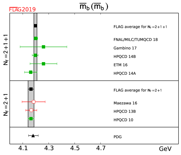
Figure 7: The $b$-quark mass, $N_{f}=2+1$ and $2+1+1$. The updated PDG value from Ref. [Tanabashi:2018oca] is reported for comparison.

4 Leptonic and semileptonic kaon and pion decay and $|V_{ud}|$ and $|V_{us}|$

Authors: T. Kaneko, J. N. Simone, S. Simula

This section summarizes state-of-the-art lattice calculations of the leptonic kaon and pion decay constants and the kaon semileptonic-decay form factor and provides an analysis in view of the Standard Model. With respect to the previous edition of the FLAG review [Aoki:2016frl] the data in this section has been updated. As in Ref. [Aoki:2016frl], when combining lattice data with experimental results, we take into account the strong $SU(2)$ isospin correction, either obtained in lattice calculations or estimated by using chiral perturbation theory ($\chi$PT), both for the kaon leptonic decay constant $f_{K^{\pm}}$ and for the ratio $f_{K^{\pm}}/f_{\pi^{\pm}}$.

4.1 Experimental information concerning $|V_{ud}|$, $|V_{us}|$, $f_{+}(0)$ and ${f_{K^{\pm}}}/{f_{\pi^{\pm}}}$

The following review relies on the fact that precision experimental data on kaon decays very accurately determine the product $|V_{us}|f_{+}(0)$ [Moulson:2017ive] and the ratio $|V_{us}/V_{ud}|f_{K^{\pm}}/f_{\pi^{\pm}}$ [Moulson:2017ive, Patrignani:2016xqp]:

$$|V_{us}|f_{+}(0)=0.2165(4)\,,\hskip 28.45274pt\;\left|\frac{V_{us}}{V_{ud}}\right|\frac{f_{K^{\pm}}}{f_{\pi^{\pm}}}\;=0.2760(4)\,.$$ (69)

Here and in the following, $f_{K^{\pm}}$ and $f_{\pi^{\pm}}$ are the isospin-broken decay constants, respectively, in QCD. We will refer to the decay constants in the $SU(2)$ isospin-symmetric limit as $f_{K}$ and $f_{\pi}$ (the latter at leading order in the mass difference ($m_{u}-m_{d}$) coincides with $f_{\pi^{\pm}}$). The parameters $|V_{ud}|$ and $|V_{us}|$ are elements of the Cabibbo-Kobayashi-Maskawa matrix and $f_{+}(q^{2})$ represents one of the form factors relevant for the semileptonic decay $K^{0}\rightarrow\pi^{-}\ell\,\nu$, which depends on the momentum transfer $q$ between the two mesons. What matters here is the value at $q^{2}=0$: $f_{+}(0)\equiv f_{+}^{K^{0}\pi^{-}}(0)=f_{0}^{K^{0}\pi^{-}}(0)=q^{\mu}\langle\pi^{-}(p^{\prime})|\bar{s}\gamma_{\mu}u|K^{0}(p)\rangle/(M_{K}^{2}-M_{\pi}^{2})\,\rule[-4.26773pt]{0.56917pt}{14.22636pt}_{\;q^{2}\rightarrow 0}$. The pion and kaon decay constants are defined by

$$\langle 0|\,\,\overline{\rule[6.49994pt]{3.99994pt}{0.0pt}}d\gamma_{\mu}\gamma_{5}\hskip 1.42271ptu|\pi^{+}(p)\rangle=i\hskip 1.42271ptp_{\mu}f_{\pi^{+}}\,,\hskip 28.45274pt\langle 0|\,\,\overline{\rule[4.19998pt]{3.99994pt}{0.0pt}}s\gamma_{\mu}\gamma_{5}\hskip 1.42271ptu|K^{+}(p)\rangle=i\hskip 1.42271ptp_{\mu}f_{K^{+}}\,.$$

In this normalization, $f_{\pi^{\pm}}\simeq 130$ MeV, $f_{K^{\pm}}\simeq 155$ MeV.

In Eq. (69), the electromagnetic effects have already been subtracted in the experimental analysis using $\chi$PT. Recently, a new method [Carrasco:2015xwa] has been proposed for calculating the leptonic decay rates of hadrons including both QCD and QED on the lattice, and successfully applied to the case of the ratio of the leptonic decay rates of kaons and pions [Giusti:2017dwk]. The correction to the tree-level $K_{\mu 2}/\pi_{\mu 2}$ decay rate, including both electromagnetic and strong isospin-breaking effects, is found to be equal to $-1.22(16)\%$ to be compared to the estimate $-1.12(21)\%$ based on $\chi$PT [Rosner:2015wva, Cirigliano:2011tm]. Using the experimental values of the $K_{\mu 2}$ and $\pi_{\mu 2}$ decay rates the result of Ref. [Giusti:2017dwk] implies

$$\left|\frac{V_{us}}{V_{ud}}\right|\frac{f_{K}}{f_{\pi}}=0.27673\,(29)_{\rm exp}\,(23)_{\rm th}\,[37]~{},$$ (70)

where the last error in brackets is the sum in quadrature of the experimental and theoretical uncertainties, and the ratio of the decay constants is the one corresponding to isosymmetric QCD. The single calculation of Ref. [Giusti:2017dwk] is clearly not ready for averaging, but it demonstrates that the determination of $V_{us}/V_{ud}$ using only lattice-QCD+QED and the ratio of the experimental values of the $K_{\mu 2}$ and $\pi_{\mu 2}$ decay rates is feasible with good accuracy.

The measurement of $|V_{ud}|$ based on superallowed nuclear $\beta$ transitions has now become remarkably precise. The result of the update of Hardy and Towner [Hardy:2016vhg], which is based on 20 different superallowed transitions, reads

$$|V_{ud}|=0.97420(21)\,.$$ (71)

The matrix element $|V_{us}|$ can be determined from semi-inclusive $\tau$ decays [Gamiz:2002nu, Gamiz:2004ar, Maltman:2008na, Pich_Kass]. By separating the inclusive decay $\tau\rightarrow\mbox{hadrons}+\nu$ into nonstrange and strange final states, e.g., HFLAV 16 [Amhis:2016xyh] obtains $|V_{us}|=0.2186(21)$ and both Maltman et al. [Maltman:2008ib, Maltman:2008na, Maltman:2009bh] and Gamiz et al. [Gamiz:2007qs, Gamiz:2013wn] arrive at very similar values. Inclusive hadronic $\tau$ decay offers an interesting way to measure $|V_{us}|$, but the above value of $|V_{us}|$ differs from the result one obtains from assuming three-flavour SM-unitarity by more than three standard deviations [Amhis:2016xyh]. This apparent tension has been recently solved in Ref. [Hudspith:2017vew] thanks to the use of a different experimental input and to a new treatment of higher orders in the operator product expansion and of violations of quark-hadron duality. A much larger value of $|V_{us}|$ is obtained, namely,

$$|V_{us}|=0.2231(27)_{\rm exp}(4)_{\rm th}~{},$$ (72)

which is in much better agreement with CKM unitarity. Recently, in Ref. [Boyle:2018ilm], a new method, which includes also the lattice calculation of the hadronic vacuum polarization function, has been proposed for the determination of $|V_{us}|$ from inclusive strange $\tau$ decays.

The experimental results in Eq. (69) are for the semileptonic decay of a neutral kaon into a negatively charged pion and the charged pion and kaon leptonic decays, respectively, in QCD. In the case of the semileptonic decays the corrections for strong and electromagnetic isospin breaking in chiral perturbation theory at NLO have allowed for averaging the different experimentally measured isospin channels [Antonelli:2010yf]. This is quite a convenient procedure as long as lattice-QCD simulations do not include strong or QED isospin-breaking effects. Several lattice results for $f_{K}/f_{\pi}$ are quoted for QCD with (squared) pion and kaon masses of $M_{\pi}^{2}=M_{\pi^{0}}^{2}$ and $M_{K}^{2}=\frac{1}{2}\left(M_{K^{\pm}}^{2}+M_{K^{0}}^{2}-M_{\pi^{\pm}}^{2}+M_{\pi^{0}}^{2}\right)$ for which the leading strong and electromagnetic isospin violations cancel. While the modern trend is to include strong and electromagnetic isospin breaking in the lattice simulations (e.g., Refs. [Aoki:2008sm, deDivitiis:2011eh, Ishikawa:2012ix, TakuLat12, deDivitiis:2013xla, Tantalo:2013maa, Portelli:2015gda, Carrasco:2015xwa, Giusti:2017dwk]), in this section contact with experimental results is made by correcting leading $SU(2)$ isospin breaking guided either by chiral perturbation theory or by lattice calculations.

4.2 Lattice results for $f_{+}(0)$ and $f_{K^{\pm}}/f_{\pi^{\pm}}$

Collaboration	Ref.	$N_{f}$	publication status	chiral extrapolation	continuum extrapolation	finite-volume errors	$f_{+}(0)$
FNAL/MILC 18	[Bazavov:2018kjg]	2+1+1	P	$\bigstar$	$\bigstar$	$\bigstar$	0.9696(15)(11)
ETM 16	[Carrasco:2016kpy]	2+1+1	A	$\circ$	$\bigstar$	$\circ$	0.9709(45)(9)
FNAL/MILC 13E	[Bazavov:2013maa]	2+1+1	A	$\bigstar$	$\bigstar$	$\bigstar$	0.9704(24)(22)
FNAL/MILC 13C	[Gamiz:2013xxa]	2+1+1	C	$\bigstar$	$\bigstar$	$\bigstar$	0.9704(24)(22)
JLQCD 17	[Aoki:2017spo]	2+1	A	$\circ$	$\blacksquare$	$\circ$	0.9636(36)(${}^{+57}_{-35}$)
RBC/UKQCD 15A	[Boyle:2015hfa]	2+1	A	$\bigstar$	$\circ$	$\circ$	0.9685(34)(14)
RBC/UKQCD 13	[Boyle:2013gsa]	2+1	A	$\bigstar$	$\circ$	$\circ$	0.9670(20)(${}^{+18}_{-46}$)
FNAL/MILC 12I	[Bazavov:2012cd]	2+1	A	$\circ$	$\circ$	$\bigstar$	0.9667(23)(33)
JLQCD 12	[Kaneko:2012cta]	2+1	C	$\circ$	$\blacksquare$	$\bigstar$	0.959(6)(5)
JLQCD 11	[Kaneko:2011rp]	2+1	C	$\circ$	$\blacksquare$	$\bigstar$	0.964(6)
RBC/UKQCD 10	[Boyle:2010bh]	2+1	A	$\circ$	$\blacksquare$	$\bigstar$	0.9599(34)(${}^{+31}_{-47}$)(14)
RBC/UKQCD 07	[Boyle:2007qe]	2+1	A	$\circ$	$\blacksquare$	$\bigstar$	0.9644(33)(34)(14)
ETM 10D	[Lubicz:2010bv]	2	C	$\circ$	$\bigstar$	$\circ$	0.9544(68)${}_{stat}$
ETM 09A	[Lubicz:2009ht]	2	A	$\circ$	$\circ$	$\circ$	0.9560(57)(62)

Table 13: Colour code for the data on $f_{+}(0)$. With respect to the previous edition [Aoki:2016frl] old results with two red tags have been dropped.

The traditional way of determining $|V_{us}|$ relies on using estimates for the value of $f_{+}(0)$, invoking the Ademollo-Gatto theorem [Ademollo_Gatto]. Since this theorem only holds to leading order of the expansion in powers of $m_{u}$, $m_{d}$, and $m_{s}$, theoretical models are used to estimate the corrections. Lattice methods have now reached the stage where quantities like $f_{+}(0)$ or $f_{K}/f_{\pi}$ can be determined to good accuracy. As a consequence, the uncertainties inherent in the theoretical estimates for the higher order effects in the value of $f_{+}(0)$ do not represent a limiting factor any more and we shall therefore not invoke those estimates. Also, we will use the experimental results based on nuclear $\beta$ decay and $\tau$ decay exclusively for comparison—the main aim of the present review is to assess the information gathered with lattice methods and to use it for testing the consistency of the SM and its potential to provide constraints for its extensions.

The database underlying the present review of the semileptonic form factor and the ratio of decay constants is listed in Tabs. 13 and 1. The properties of the lattice data play a crucial role for the conclusions to be drawn from these results: range of $M_{\pi}$, size of $LM_{\pi}$, continuum extrapolation, extrapolation in the quark masses, finite-size effects, etc. The key features of the various data sets are characterized by means of the colour code specified in Sec. 2.1. Note that with respect to the previous edition [Aoki:2016frl] we have dropped old results with two red tags. More detailed information on individual computations are compiled in Appendix LABEL:app:VusVud, which in this edition is limited to new results and to those entering the FLAG averages. For other calculations the reader should refer to the Appendix B.2 of Ref. [Aoki:2016frl].

The quantity $f_{+}(0)$ represents a matrix element of a strangeness-changing null-plane charge, $f_{+}(0)=\langle K|Q^{\bar{u}s}|\pi\rangle$ (see Ref. [Gasser:1984ux]). The vector charges obey the commutation relations of the Lie algebra of $SU(3)$, in particular $[Q^{\bar{u}s},Q^{\bar{s}u}]=Q^{\bar{u}u-\bar{s}s}$. This relation implies the sum rule $\sum_{n}|\langle K|Q^{\bar{u}s}|n\rangle|^{2}-\sum_{n}|\langle K|Q^{\bar{s}u}|n\rangle|^{2}=1$. Since the contribution from the one-pion intermediate state to the first sum is given by $f_{+}(0)^{2}$, the relation amounts to an exact representation for this quantity [Furlan]:

$$f_{+}(0)^{2}=1-\sum_{n\neq\pi}|\langle K|Q^{\bar{u}s}|n\rangle|^{2}+\sum_{n}|\langle K|Q^{\bar{s}u}|n\rangle|^{2}\,.$$ (73)

While the first sum on the right extends over nonstrange intermediate states, the second runs over exotic states with strangeness $\pm 2$ and is expected to be small compared to the first.

The expansion of $f_{+}(0)$ in $SU(3)$ chiral perturbation theory in powers of $m_{u}$, $m_{d}$, and $m_{s}$ starts with $f_{+}(0)=1+f_{2}+f_{4}+\ldots\,$ [Gasser:1984gg]. Since all of the low-energy constants occurring in $f_{2}$ can be expressed in terms of $M_{\pi}$, $M_{K}$, $M_{\eta}$ and $f_{\pi}$ [Gasser:1984ux], the NLO correction is known. In the language of the sum rule (73), $f_{2}$ stems from nonstrange intermediate states with three mesons. Like all other nonexotic intermediate states, it lowers the value of $f_{+}(0)$: $f_{2}=-0.023$ when using the experimental value of $f_{\pi}$ as input. The corresponding expressions have also been derived in quenched or partially quenched (staggered) chiral perturbation theory [Bernard:2013eya, Bazavov:2012cd]. At the same order in the $SU(2)$ expansion [Flynn:2008tg], $f_{+}(0)$ is parameterized in terms of $M_{\pi}$ and two a priori unknown parameters. The latter can be determined from the dependence of the lattice results on the masses of the quarks. Note that any calculation that relies on the $\chi$PT formula for $f_{2}$ is subject to the uncertainties inherent in NLO results: instead of using the physical value of the pion decay constant $f_{\pi}$, one may, for instance, work with the constant $f_{0}$ that occurs in the effective Lagrangian and represents the value of $f_{\pi}$ in the chiral limit. Although trading $f_{\pi}$ for $f_{0}$ in the expression for the NLO term affects the result only at NNLO, it may make a significant numerical difference in calculations where the latter are not explicitly accounted for. (Lattice results concerning the value of the ratio $f_{\pi}/f_{0}$ are reviewed in Sec. 5.3.)

\psfrag{y}{\tiny$\star$}\includegraphics[height=177.82971pt]{Vudus/Figures/f+0}

\psfrag{y}{\tiny$\star$}\includegraphics[height=177.82971pt]{Vudus/Figures/RfKfpi}

[Kastner:2008ch]

[Cirigliano:2005xn]

[Jamin:2004re]

[Bijnens:2003uy]

[Leutwyler:1984je]

Figure 8: Comparison of lattice results (squares) for $f_{+}(0)$ and $f_{K^{\pm}}/f_{\pi^{\pm}}$ with various model estimates based on $\chi$PT (blue circles). The ratio $f_{K^{\pm}}/f_{\pi^{\pm}}$ is obtained in pure QCD including the $SU(2)$ isospin-breaking correction (see Sec. 4.3). The black squares and grey bands indicate our estimates. The significance of the colours is explained in Sec. 2.

The lattice results shown in the left panel of Fig. 8 indicate that the higher order contributions $\Delta f\equiv f_{+}(0)-1-f_{2}$ are negative and thus amplify the effect generated by $f_{2}$. This confirms the expectation that the exotic contributions are small. The entries in the lower part of the left panel represent various model estimates for $f_{4}$. In Ref. [Leutwyler:1984je], the symmetry-breaking effects are estimated in the framework of the quark model. The more recent calculations are more sophisticated, as they make use of the known explicit expression for the $K_{\ell 3}$ form factors to NNLO in $\chi$PT [Post:2001si, Bijnens:2003uy]. The corresponding formula for $f_{4}$ accounts for the chiral logarithms occurring at NNLO and is not subject to the ambiguity mentioned above. The numerical result, however, depends on the model used to estimate the low-energy constants occurring in $f_{4}$ [Bijnens:2003uy, Jamin:2004re, Cirigliano:2005xn, Kastner:2008ch]. The figure indicates that the most recent numbers obtained in this way correspond to a positive or an almost vanishing rather than a negative value for $\Delta f$. We note that FNAL/MILC 12I [Bazavov:2012cd] and Ref. [Bernard:2007tk] have made an attempt at determining a combination of some of the low-energy constants appearing in $f_{4}$ from lattice data.

4.3 Direct determination of $f_{+}(0)$ and $f_{K^{\pm}}/f_{\pi^{\pm}}$

Many lattice results for the form factor $f_{+}(0)$ and for the ratio of decay constants, which we summarize here in Tabs. 13 and 1, respectively, have been computed in isospin-symmetric QCD. The reason for this unphysical parameter choice is that there are only a few simulations of isospin-breaking effects in lattice QCD, which is ultimately the cleanest way for predicting these effects  [Duncan:1996xy, Basak:2008na, Blum:2010ym, Portelli:2010yn, deDivitiis:2011eh, deDivitiis:2013xla, Tantalo:2013maa, Portelli:2015gda, Carrasco:2015xwa, Giusti:2017dwk]. In the meantime, one relies either on chiral perturbation theory [Gasser:1984gg, Aubin:2004fs] to estimate the correction to the isospin limit or one calculates the breaking at leading order in $(m_{u}-m_{d})$ in the valence quark sector by extrapolating the lattice data for the charged kaons to the physical value of the $up$($down$)-quark mass (the result for the pion decay constant is always extrapolated to the value of the average light-quark mass $\hat{m}$). This defines the prediction for $f_{K^{\pm}}/f_{\pi^{\pm}}$.

• Result with statistical error only from polynomial interpolation to the physical point.
  

• This work is the continuation of Aubin 08.

Table 14: Colour code for the data on the ratio of decay constants: $f_{K}/f_{\pi}$ is the pure QCD $SU(2)$-symmetric ratio, while $f_{K^{\pm}}/f_{\pi^{\pm}}$ is in pure QCD including the $SU(2)$ isospin-breaking correction. With respect to the previous edition [Aoki:2016frl] old results with two red tags have been dropped.

Since the majority of results that qualify for inclusion into the FLAG average include the strong $SU(2)$ isospin-breaking correction, we confirm the choice made in the previous edition of the FLAG review [Aoki:2016frl] and we provide in Fig. 8 the overview of the world data of $f_{K^{\pm}}/f_{\pi^{\pm}}$. For all the results of Tab. 1 provided only in the isospin-symmetric limit we apply individually an isospin correction that will be described later on (see Eqs. (78-79)).

The plots in Fig. 8 illustrate our compilation of data for $f_{+}(0)$ and $f_{K^{\pm}}/f_{\pi^{\pm}}$. The lattice data for the latter quantity is largely consistent even when comparing simulations with different $N_{f}$, while in the case of $f_{+}(0)$ a slight tendency to get higher values for increasing $N_{f}$ seems to be visible, even if it does not exceed one standard deviation. We now proceed to form the corresponding averages, separately for the data with $N_{f}=2+1+1$, $N_{f}=2+1$, and $N_{f}=2$ dynamical flavours, and in the following we will refer to these averages as the “direct” determinations.

4.3.1 Results for $f_{+}(0)$

For $f_{+}(0)$ there are currently two computational strategies: FNAL/MILC uses the Ward identity to relate the $K\to\pi$ form factor at zero momentum transfer to the matrix element $\langle\pi|S|K\rangle$ of the flavour-changing scalar current $S=\bar{s}u$. Peculiarities of the staggered fermion discretization used by FNAL/MILC (see Ref. [Bazavov:2012cd]) makes this the favoured choice. The other collaborations are instead computing the vector current matrix element $\langle\pi|\bar{s}\gamma_{\mu}u|K\rangle$. Apart from FNAL/MILC 13C, FNAL/MILC 13E and RBC/UKQCD 15A all simulations in Tab. 13 involve unphysically heavy quarks and, therefore, the lattice data needs to be extrapolated to the physical pion and kaon masses corresponding to the $K^{0}\to\pi^{-}$ channel. We note also that the recent computations of $f_{+}(0)$ obtained by the FNAL/MILC and RBC/UKQCD collaborations make use of the partially-twisted boundary conditions to determine the form-factor results directly at the relevant kinematical point $q^{2}=0$ [Guadagnoli:2005be, Boyle:2007wg], avoiding in this way any uncertainty due to the momentum dependence of the vector and/or scalar form factors. The ETM collaboration uses partially-twisted boundary conditions to compare the momentum dependence of the scalar and vector form factors with the one of the experimental data [Lubicz:2010bv, Carrasco:2016kpy], while keeping at the same time the advantage of the high-precision determination of the scalar form factor at the kinematical end-point $q_{max}^{2}=(M_{K}-M_{\pi})^{2}$ [Becirevic:2004ya, Lubicz:2009ht] for the interpolation at $q^{2}=0$.

According to the colour codes reported in Tab. 13 and to the FLAG rules of Sec. 2.2, only the result ETM 09A with $N_{f}=2$, the results FNAL/MILC 12I and RBC/UKQCD 15A with $N_{f}=2+1$ and the results FNAL/MILC 13E and ETM 16 with $N_{f}=2+1+1$ dynamical flavours of fermions, respectively, can enter the FLAG averages.

At $N_{f}=2+1+1$ the result from the FNAL/MILC collaboration, $f_{+}(0)=0.9704(24)(22)$ (FNAL/MILC 13E), is based on the use of the Highly Improved Staggered Quark (HISQ) action (for both valence and sea quarks), which has been tailored to reduce staggered taste-breaking effects, and includes simulations with three lattice spacings and physical light-quark masses. These features allow to keep the uncertainties due to the chiral extrapolation and to the discretization artifacts well below the statistical error. The remaining largest systematic uncertainty comes from finite-size effects, which have been investigated in Ref. [Bernard:2017scg] using 1-loop $\chi$PT (with and without taste-violating effects). Recently [Bazavov:2018kjg] the FNAL/MILC collaboration presented a more precise determination of $f_{+}(0)$, $f_{+}(0)=0.9696(15)(11)$ (see the entry FNAL/MILC 18 in Tab. 13), in which the improvement of the precision with respect to FNAL/MILC 13E is obtained mainly by using an estimate of finite-size effects based on ChPT only. We do not consider FNAL/MILC 18 as a plain update of FNAL/MILC 13E.

The new result from the ETM collaboration, $f_{+}(0)=0.9709(45)(9)$ (ETM 16), makes use of the twisted-mass discretization adopting three values of the lattice spacing in the range $0.06-0.09$ fm and pion masses simulated in the range $210-450$ MeV. The chiral and continuum extrapolations are performed in a combined fit together with the momentum dependence, using both a $SU(2)$-$\chi$PT inspired ansatz (following Ref. [Lubicz:2010bv]) and a modified z-expansion fit. The uncertainties coming from the chiral extrapolation, the continuum extrapolation and the finite-volume effects turn out to be well below the dominant statistical error, which includes also the error due to the fitting procedure. A set of synthetic data points, representing both the vector and the scalar semileptonic form factors at the physical point for several selected values of $q^{2}$, is provided together with the corresponding correlation matrix.

At $N_{f}=2+1$ there is a new result from the JLQCD collaboration [Aoki:2017spo], which however does not satisfy all FLAG criteria for entering the average. The two results eligible to enter the FLAG average at $N_{f}=2+1$ are the one from RBC/UKQCD 15A, $f_{+}(0)=0.9685(34)(14)$ [Boyle:2015hfa], and the one from FNAL/MILC 12I, $f_{+}(0)=0.9667(23)(33)$ [Bazavov:2012cd]. These results, based on different fermion discretizations (staggered fermions in the case of FNAL/MILC and domain wall fermions in the case of RBC/UKQCD) are in nice agreement. Moreover, in the case of FNAL/MILC the form factor has been determined from the scalar current matrix element, while in the case of RBC/UKQCD it has been determined including also the matrix element of the vector current. To a certain extent both simulations are expected to be affected by different systematic effects.

RBC/UKQCD 15A has analyzed results on ensembles with pion masses down to 140 MeV, mapping out the complete range from the $SU(3)$-symmetric limit to the physical point. No significant cut-off effects (results for two lattice spacings) were observed in the simulation results. Ensembles with unphysical light-quark masses are weighted to work as a guide for small corrections toward the physical point, reducing in this way the model dependence in the fitting ansatz. The systematic uncertainty turns out to be dominated by finite-volume effects, for which an estimate based on effective theory arguments is provided.

The result FNAL/MILC 12I is from simulations reaching down to a lightest RMS pion mass of about 380 MeV (the lightest valence pion mass for one of their ensembles is about 260 MeV). Their combined chiral and continuum extrapolation (results for two lattice spacings) is based on NLO staggered chiral perturbation theory supplemented by the continuum NNLO expression [Bijnens:2003uy] and a phenomenological parameterization of the breaking of the Ademollo-Gatto theorem at finite lattice spacing inherent in their approach. The $p^{4}$ low-energy constants entering the NNLO expression have been fixed in terms of external input [Amoros:2001cp].

The ETM collaboration uses the twisted-mass discretization and provides at $N_{f}=2$ a comprehensive study of the systematics [Lubicz:2009ht, Lubicz:2010bv], by presenting results for four lattice spacings and by simulating at light pion masses (down to $M_{\pi}=260$ MeV). This makes it possible to constrain the chiral extrapolation, using both $SU(3)$ [Gasser:1984ux] and $SU(2)$ [Flynn:2008tg] chiral perturbation theory. Moreover, a rough estimate for the size of the effects due to quenching the strange quark is given, based on the comparison of the result for $N_{f}=2$ dynamical quark flavours [Blossier:2009bx] with the one in the quenched approximation, obtained earlier by the SPQcdR collaboration [Becirevic:2004ya].

We now compute the $N_{f}=2+1+1$ FLAG-average for $f_{+}(0)$ using the FNAL/MILC 13E and ETM 16 (uncorrelated) results, the $N_{f}=2+1$ FLAG-average based on FNAL/MILC 12I and RBC/UKQCD 15A, which we consider uncorrelated, while for $N_{f}=2$ we consider directly the ETM 09A result, respectively:

$$\mbox{direct},\,N_{f}=2+1+1: f_{+}(0) =0.9706(27) \,\mathrm{Refs.}~{}\mbox{\cite[cite]{[\@@bibref{Number}{Bazavov:2013maa,Carrasco:2016kpy}{}{}]}},$$ (74)

$$\mbox{direct},\,N_{f}=2+1: f_{+}(0) =0.9677(27) \,\mathrm{Refs.}~{}\mbox{\cite[cite]{[\@@bibref{Number}{Bazavov:2012cd,Boyle:2015hfa}{}{}]}},$$ (75)

$$\mbox{direct},\,N_{f}=2: f_{+}(0) =0.9560(57)(62) \ref{~}\mbox{\cite[cite]{[\@@bibref{Number}{Lubicz:2009ht}{}{}]}},$$ (76)

where the brackets in the third line indicate the statistical and systematic errors, respectively. We stress that the results (74) and (75), corresponding to $N_{f}=2+1+1$ and $N_{f}=2+1$, respectively, include already simulations with physical light-quark masses.

4.3.2 Results for $f_{K^{\pm}}/f_{\pi^{\pm}}$

In the case of the ratio of decay constants the data sets that meet the criteria formulated in the introduction are HPQCD 13A [Dowdall:2013rya], ETM 14E [Carrasco:2014poa] and FNAL/MILC 17 [Bazavov:2017lyh] (which updates FNAL/MILC 14A [Bazavov:2014wgs]) with $N_{f}=2+1+1$, HPQCD/UKQCD 07 [Follana:2007uv], MILC 10 [Bazavov:2010hj], BMW 10 [Durr:2010hr], RBC/UKQCD 14B [Blum:2014tka], Dürr 16 [Durr:2016ulb, Scholz:2016kcr] and QCDSF/UKQCD 16 [Bornyakov:2016dzn] with $N_{f}=2+1$ and ETM 09 [Blossier:2009bx] with $N_{f}=2$ dynamical flavours.

ETM 14E uses the twisted-mass discretization and provides a comprehensive study of the systematics by presenting results for three lattice spacings in the range $0.06-0.09$ fm and for pion masses in the range $210-450$ MeV. This makes it possible to constrain the chiral extrapolation, using both $SU(2)$ [Flynn:2008tg] chiral perturbation theory and polynomial fits. The ETM collaboration always includes the spread in the central values obtained from different ansätze into the systematic errors. The final result of their analysis is ${f_{K^{\pm}}}/{f_{\pi^{\pm}}}=1.184(12)_{\rm stat+fit}(3)_{\rm Chiral}(9)_{\rm a^{2}}(1)_{Z_{P}}(3)_{FV}(3)_{IB}$ where the errors are (statistical + the error due to the fitting procedure), due to the chiral extrapolation, the continuum extrapolation, the mass-renormalization constant, the finite-volume and (strong) isospin-breaking effects.

FNAL/MILC 17 [Bazavov:2017lyh] has determined the ratio of the decay constants from a comprehensive set of HISQ ensembles with $N_{f}=2+1+1$ dynamical flavours. They have generated 24 ensembles for six values of the lattice spacing ($0.03-0.15$ fm, scale set with $f_{\pi^{+}}$) and with both physical and unphysical values of the light sea-quark masses, controlling in this way the systematic uncertainties due to chiral and continuum extrapolations. With respect to FNAL/MILC 14A they have increased the statistics and added three ensembles at very fine lattice spacings, $a\simeq 0.03$ and $0.042$ fm, including for the latter case also a simulation at the physical value of the light-quark mass. The final result of their analysis is ${f_{K^{\pm}}}/{f_{\pi^{\pm}}}=1.1950(14)_{\rm stat}($${}_{-17}^{+0}$$)_{\rm a^{2}}(2)_{FV}(3)_{f_{\pi},PDG}(3)_{EM}(2)_{Q^{2}}$, where the errors are statistical, due to the continuum extrapolation, finite-volume, pion decay constant from PDG, electromagnetic effects and sampling of the topological charge distribution.

HPQCD 13A has analyzed ensembles generated by MILC and therefore its study of ${f_{K^{\pm}}}/{f_{\pi^{\pm}}}$ is based on the same set of ensembles bar the ones at the finest lattice spacings (namely, only $a=0.09-0.15$ fm, scale set with $f_{\pi^{+}}$ and relative scale set with the Wilson flow [Luscher:2010iy, Borsanyi:2012zs]) supplemented by some simulation points with heavier quark masses. HPQCD employs a global fit based on continuum NLO $SU(3)$ chiral perturbation theory for the decay constants supplemented by a model for higher-order terms including discretization and finite-volume effects (61 parameters for 39 data points supplemented by Bayesian priors). Their final result is $f_{K^{\pm}}/f_{\pi^{\pm}}=1.1916(15)_{\rm stat}(12)_{\rm a^{2}}(1)_{FV}(10)$, where the errors are statistical, due to the continuum extrapolation, due to finite-volume effects and the last error contains the combined uncertainties from the chiral extrapolation, the scale-setting uncertainty, the experimental input in terms of $f_{\pi^{+}}$ and from the uncertainty in $m_{u}/m_{d}$.

In the two previous editions of the FLAG review [Aoki:2013ldr, Aoki:2016frl] the error budget of HPQCD 13A was compared with the ones of MILC 13A and FNAL/MILC 14A and discussed in detail. It was pointed out that, despite the overlap in primary lattice data, both collaborations arrive at surprisingly different error budgets, particularly in the cases of the cutoff dependence and of the finite volume effects. The error budget of the latest update FNAL/MILC 17, which has a richer lattice setup with respect to HPQCD 13A, is consistent with the one of HPQCD 13A.

Adding in quadrature all the uncertainties one gets: $f_{K^{\pm}}/f_{\pi^{\pm}}=1.1916(22)$ (HPQCD 13A) and ${f_{K^{\pm}}}/{f_{\pi^{\pm}}}=1.1944(18)$ (FNAL/MILC 17). It can be seen that the total errors are very similar and the central values are consistent within approximately one standard deviation. Thus, the HPQCD 13A and FNAL/MILC 17 are averaged, assuming a $100\%$ statistical and systematic correlations between them, together with the (uncorrelated) ETM 14E result, obtaining

$$\mbox{direct},\,N_{f}=2+1+1: \quad\quad{f_{K^{\pm}}}/{f_{\pi^{\pm}}}=1.1932(19) \,\mathrm{Refs.}~{}\mbox{\cite[cite]{[\@@bibref{Number}{Dowdall:2013rya,Carrasco:2014poa,Bazavov:2017lyh}{}{}]}}\,.$$ (77)

For $N_{f}=2+1$ the result Dürr 16 [Durr:2016ulb, Scholz:2016kcr] is now eligible to enter the FLAG average as well as the new result [Bornyakov:2016dzn] from the QCDSF collaboration. Dürr 16 [Durr:2016ulb, Scholz:2016kcr] has analyzed the decay constants evaluated for 47 gauge ensembles generated using tree-level clover-improved fermions with two HEX-smearings and the tree-level Symanzik-improved gauge action. The ensembles correspond to five values of the lattice spacing ($0.05-0.12$ fm, scale set by $\Omega$ mass), to pion masses in the range $130-680$ MeV and to values of the lattice size from $1.7$ to $5.6$ fm, obtaining a good control over the interpolation to the physical mass point and the extrapolation to the continuum and infinite volume limits.

QCDSF/UKQCD 16 [Bornyakov:2016dzn] has used the nonperturbatively ${\cal{O}}(a)$-improved clover action for the fermions (mildly stout-smeared) and the tree-level Symanzik action for the gluons. Four values of the lattice spacing ($0.06-0.08$ fm) have been simulated with pion masses down to $\sim 220$ MeV and values of the lattice size in the range $2.0-2.8$ fm. The decay constants are evaluated using an expansion around the symmetric $SU(3)$ point $m_{u}=m_{d}=m_{s}=(m_{u}+m_{d}+m_{s})^{phys}/3$.

Note that for $N_{f}=2+1$ MILC 10 and HPQCD/UKQCD 07 are based on staggered fermions, BMW 10, Dürr 16 and QCDSF/UKQCD 16 have used improved Wilson fermions and RBC/UKQCD 14B’s result is based on the domain-wall formulation. In contrast to RBC/UKQCD 14B and Dürr 16 the other simulations are for unphysical values of the light-quark masses (corresponding to smallest pion masses in the range $220-260$ MeV in the case of MILC 10, HPQCD/UKQCD 07 and QCDSF/UKQCD 16) and therefore slightly more sophisticated extrapolations needed to be controlled. Various ansätze for the mass and cutoff dependence comprising $SU(2)$ and $SU(3)$ chiral perturbation theory or simply polynomials were used and compared in order to estimate the model dependence. While BMW 10, RBC/UKQCD 14B and QCDSF/UKQCD 16 are entirely independent computations, subsets of the MILC gauge ensembles used by MILC 10 and HPQCD/UKQCD 07 are the same. MILC 10 is certainly based on a larger and more advanced set of gauge configurations than HPQCD/UKQCD 07. This allows them for a more reliable estimation of systematic effects. In this situation we consider both statistical and systematic uncertainties to be correlated.

For $N_{f}=2$ no new result enters the corresponding FLAG average with respect to the previous edition of the FLAG review [Aoki:2016frl], which therefore remains the ETM 09 result, which has simulated twisted-mass fermions down to (charged) pion masses equal to 260 MeV.

We note that the overall uncertainties quoted by ETM 14E at $N_{f}=2+1+1$ and by Dürr 16 and QCDSF/UKQCD 16 at $N_{f}=2+1$ are much larger than the overall uncertainties obtained with staggered (HPQCD 13A, FNAL/MILC 17 at $N_{f}=2+1+1$ and MILC 10, HPQCD/UKQCD 07 at $N_{f}=2+1$) and domain-wall fermions (RBC/UKQCD 14B at $N_{f}=2+1$).

Before determining the average for $f_{K^{\pm}}/f_{\pi^{\pm}}$, which should be used for applications to Standard Model phenomenology, we apply the strong isospin correction individually to all those results that have been published only in the isospin-symmetric limit, i.e., BMW 10, HPQCD/UKQCD 07 and RBC/UKQCD 14B at $N_{f}=2+1$ and ETM 09 at $N_{f}=2$. To this end, as in the previous edition of the FLAG reviews [Aoki:2013ldr, Aoki:2016frl], we make use of NLO $SU(3)$ chiral perturbation theory [Gasser:1984gg, Cirigliano:2011tm], which predicts

$$\frac{f_{K^{\pm}}}{f_{\pi^{\pm}}}=\frac{f_{K}}{f_{\pi}}~{}\sqrt{1+\delta_{SU(2)}}~{},$$ (78)

where [Cirigliano:2011tm]

$$\begin{array}[]{rcl}\delta_{SU(2)}&\approx&\sqrt{3}\,\epsilon_{SU(2)}\left[-\frac{4}{3}\left(f_{K}/f_{\pi}-1\right)+\frac{2}{3(4\pi)^{2}f_{0}^{2}}\left(M_{K}^{2}-M_{\pi}^{2}-M_{\pi}^{2}\ln\frac{M_{K}^{2}}{M_{\pi}^{2}}\right)\right]\,.\end{array}$$ (79)

We use as input $\epsilon_{SU(2)}=\sqrt{3}/(4R)$ with the FLAG result for $R$ of Eq. (54), $F_{0}=f_{0}/\sqrt{2}=80\,(20)$ MeV, $M_{\pi}=135$ MeV and $M_{K}=495$ MeV (we decided to choose a conservative uncertainty on $f_{0}$ in order to reflect the magnitude of potential higher-order corrections). The results are reported in Tab. 15, where in the last column the last error is due to the isospin correction (the remaining errors are quoted in the same order as in the original data).

	$f_{K}/f_{\pi}$	$\delta_{SU(2)}$	$f_{K^{\pm}}/f_{\pi^{\pm}}$
HPQCD/UKQCD 07	1.189(2)(7)	-0.0040(7)	1.187(2)(7)(2)
BMW 10	1.192(7)(6)	-0.0041(7)	1.190(7)(6)(2)
RBC/UKQCD 14B	1.1945(45)	-0.0043(9)	1.1919(45)(26)

Table 15: Values of the $SU(2)$ isospin-breaking correction $\delta_{SU(2)}$ applied to the lattice data for $f_{K}/f_{\pi}$ , entering the FLAG average at $N_{f}=2+1$, for obtaining the corrected charged ratio $f_{K^{\pm}}/f_{\pi^{\pm}}$.

For $N_{f}=2$ and $N_{f}=2+1+1$ dedicated studies of the strong-isospin correction in lattice QCD do exist. The updated $N_{f}=2$ result of the RM123 collaboration [deDivitiis:2013xla] amounts to $\delta_{SU(2)}=-0.0080(4)$ and we use this result for the isospin correction of the ETM 09 result. Note that the above RM123 value for the strong-isospin correction is incompatible with the results based on $SU(3)$ chiral perturbation theory, $\delta_{SU(2)}=-0.004(1)$ (see Tab. 15). Moreover, for $N_{f}=2+1+1$ HPQCD [Dowdall:2013rya], FNAL/MILC [Bazavov:2017lyh] and ETM [Giusti:2017xrv] estimate a value for $\delta_{SU(2)}$ equal to $-0.0054(14)$, $-0.0052(9)$ and $-0.0073(6)$, respectively. Note that the RM123 and ETM results are obtained using the insertion of the isovector scalar current according to the expansion method of Ref. [deDivitiis:2011eh], while the HPQCD and FNAL/MILC results correspond to the difference between the values of the decay constant ratio extrapolated to the physical $u$-quark mass $m_{u}$ and to the average $(m_{u}+m_{d})/2$ light-quark mass.

One would not expect the strange and heavier sea-quark contributions to be responsible for such a large effect. Whether higher-order effects in chiral perturbation theory or other sources are responsible still needs to be understood. More lattice-QCD simulations of $SU(2)$ isospin-breaking effects are therefore required. To remain on the conservative side we add a $100\%$ error to the correction based on $SU(3)$ chiral perturbation theory. For further analyses we add (in quadrature) such an uncertainty to the systematic error.

Using the results of Tab. 15 for $N_{f}=2+1$ we obtain

$$\mbox{direct},\,N_{f}=2+1+1: f_{K^{\pm}}/f_{\pi^{\pm}} =1.1932(19) \,\mathrm{Refs.}~{}\mbox{\cite[cite]{[\@@bibref{Number}{Dowdall:2013rya,Carrasco:2014poa,Bazavov:2017lyh}{}{}]}},$$ (80)

$$\mbox{direct},\,N_{f}=2+1: f_{K^{\pm}}/f_{\pi^{\pm}} =1.1917(37) \,\mathrm{Refs.}~{}\mbox{\cite[cite]{[\@@bibref{Number}{Follana:2007uv,Bazavov:2010hj,Durr:2010hr,Blum:2014tka,Durr:2016ulb,Bornyakov:2016dzn}{}{}]}},$$ (81)

$$\mbox{direct},\,N_{f}=2: f_{K^{\pm}}/f_{\pi^{\pm}} =1.205(18) \ref{~}\mbox{\cite[cite]{[\@@bibref{Number}{Blossier:2009bx}{}{}]}},$$ (82)

for QCD with broken isospin.

The averages obtained for $f_{+}(0)$ and ${f_{K^{\pm}}}/{f_{\pi^{\pm}}}$ at $N_{f}=2+1$ and $N_{f}=2+1+1$ [see Eqs. (74-75) and (80-81)] exhibit a precision better than $\sim 0.3\%$. At such a level of precision QED effects cannot be ignored and a consistent lattice treatment of both QED and QCD effects in leptonic and semileptonic decays becomes mandatory.

4.3.3 Extraction of $|V_{ud}|$ and $|V_{us}|$

It is instructive to convert the averages for $f_{+}(0)$ and ${f_{K^{\pm}}}/{f_{\pi^{\pm}}}$ into a corresponding range for the CKM matrix elements $|V_{ud}|$ and $|V_{us}|$, using the relations (69). Consider first the results for $N_{f}=2+1+1$. The range for $f_{+}(0)$ in Eq. (74) is mapped into the interval $|V_{us}|=0.2231(7)$, depicted as a horizontal red band in Fig. 9, while the one for ${f_{K^{\pm}}}/{f_{\pi^{\pm}}}$ in Eq. (80) is converted into $|V_{us}|/|V_{ud}|=0.2313(5)$, shown as a tilted red band. The red ellipse is the intersection of these two bands and represents the 68% likelihood contour, obtained by treating the above two results as independent measurements. Repeating the exercise for $N_{f}=2+1$ leads to the green ellipse. The plot indicates a slight tension of both the $N_{f}=2+1+1$ and $N_{f}=2+1$ results with the one from nuclear $\beta$ decay.

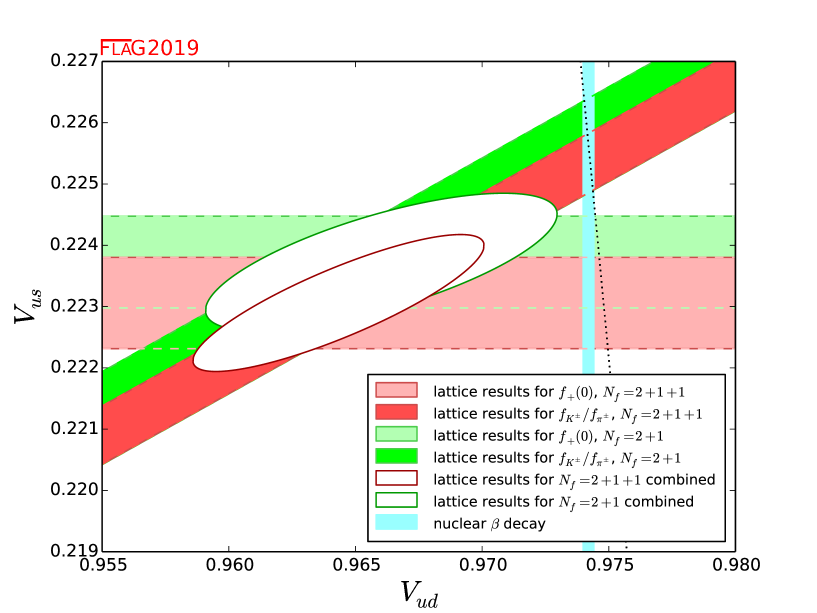
Figure 9: The plot compares the information for $|V_{ud}|$, $|V_{us}|$ obtained on the lattice for $N_{f}=2+1$ and $N_{f}=2+1+1$ with the experimental result extracted from nuclear $\beta$ transitions. The dotted line indicates the correlation between $|V_{ud}|$ and $|V_{us}|$ that follows if the CKM-matrix is unitary. For the $N_{f}=2$ results see the previous FLAG edition [Aoki:2016frl].

4.4 Tests of the Standard Model

In the Standard Model, the CKM matrix is unitary. In particular, the elements of the first row obey

$$|V_{u}|^{2}\equiv|V_{ud}|^{2}+|V_{us}|^{2}+|V_{ub}|^{2}=1\,.$$ (83)

The tiny contribution from $|V_{ub}|$ is known much better than needed in the present context: $|V_{ub}|=3.94(36)\cdot 10^{-3}$ [Patrignani:2016xqp]. In the following, we first discuss the evidence for the validity of the relation (83) and only then use it to analyse the lattice data within the Standard Model.

In Fig. 9, the correlation between $|V_{ud}|$ and $|V_{us}|$ imposed by the unitarity of the CKM matrix is indicated by a dotted line (more precisely, in view of the uncertainty in $|V_{ub}|$, the correlation corresponds to a band of finite width, but the effect is too small to be seen here). The plot shows that there is a slight tension with unitarity in the data for $N_{f}=2+1+1$: Numerically, the outcome for the sum of the squares of the first row of the CKM matrix reads $|V_{u}|^{2}=0.9797(74)$, which deviates from unity at the level of $\simeq 2.7$ standard deviations. Still, it is fair to say that at this level the Standard Model passes a nontrivial test that exclusively involves lattice data and well-established kaon decay branching ratios. Combining the lattice results for $f_{+}(0)$ and ${f_{K^{\pm}}}/{f_{\pi^{\pm}}}$ in Eqs. (74) and (80) with the $\beta$ decay value of $|V_{ud}|$ quoted in Eq. (71), the test sharpens considerably: the lattice result for $f_{+}(0)$ leads to $|V_{u}|^{2}=0.99884(53)$, which highlights again a $\simeq 2.2\sigma$-tension with unitarity, while the one for ${f_{K^{\pm}}}/{f_{\pi^{\pm}}}$ implies $|V_{u}|^{2}=0.99986(46)$, confirming the first-row CKM unitarity below the permille level. Note that the largest contribution to the uncertainty on $|V_{u}|^{2}$ comes from the error on $|V_{ud}|$ given in Eq. (71).

The situation is similar for $N_{f}=2+1$: with the lattice data alone one has $|V_{u}|^{2}=0.9832(89)$, which deviates from unity at the level of $\simeq 1.9$ standard deviations. Combining the lattice results for $f_{+}(0)$ and ${f_{K^{\pm}}}/{f_{\pi^{\pm}}}$ in Eqs. (75) and (81) with the $\beta$ decay value of $|V_{ud}|$, the test sharpens again considerably: the lattice result for $f_{+}(0)$ leads to $|V_{u}|^{2}=0.99914(53)$, implying only a $\simeq 1.6\sigma$-tension with unitarity, while the one for ${f_{K^{\pm}}}/{f_{\pi^{\pm}}}$ implies $|V_{u}|^{2}=0.99999(54)$, thus confirming again CKM unitarity below the permille level.

For the analysis corresponding to $N_{f}=2$ the reader should refer to the previous FLAG edition [Aoki:2016frl].

Note that the above tests also offer a check of the basic hypothesis that underlies our analysis: we are assuming that the weak interaction between the quarks and the leptons is governed by the same Fermi constant as the one that determines the strength of the weak interaction among the leptons and the lifetime of the muon. In certain modifications of the Standard Model, this is not the case and it need not be true that the rates of the decays $\pi\rightarrow\ell\nu$, $K\rightarrow\ell\nu$ and $K\rightarrow\pi\ell\nu$ can be used to determine the matrix elements $|V_{ud}f_{\pi}|$, $|V_{us}f_{K}|$ and $|V_{us}f_{+}(0)|$, respectively, and that $|V_{ud}|$ can be measured in nuclear $\beta$ decay. The fact that the lattice data is consistent with unitarity and with the value of $|V_{ud}|$ found in nuclear $\beta$ decay indirectly also checks the equality of the Fermi constants.

4.5 Analysis within the Standard Model

The Standard Model implies that the CKM matrix is unitary. The precise experimental constraints quoted in (69) and the unitarity condition (83) then reduce the four quantities $|V_{ud}|,|V_{us}|,f_{+}(0),{f_{K^{\pm}}}/{f_{\pi^{\pm}}}$ to a single unknown: any one of these determines the other three within narrow uncertainties.

As Fig. 10 shows, the results obtained for $|V_{us}|$ and $|V_{ud}|$ from the data on ${f_{K^{\pm}}}/{f_{\pi^{\pm}}}$ (squares) are quite consistent with the determinations via $f_{+}(0)$ (triangles). In order to calculate the corresponding average values, we restrict ourselves to those determinations that we have considered best in Sec. 4.3. The corresponding results for $|V_{us}|$ are listed in Tab. 16 (the error in the experimental numbers used to convert the values of $f_{+}(0)$ and ${f_{K^{\pm}}}/{f_{\pi^{\pm}}}$ into values for $|V_{us}|$ is included in the statistical error).

\psfrag{y}{\tiny$\star$}\includegraphics[width=460.93456pt]{Vudus/Figures/Vusud}

[Amhis:2016xyh]

[Hudspith:2017vew]

[Hudspith:2017vew]

[Hardy:2016vhg]

Figure 10: Results for $|V_{us}|$ and $|V_{ud}|$ that follow from the lattice data for $f_{+}(0)$ (triangles) and ${f_{K^{\pm}}}/{f_{\pi^{\pm}}}$ (squares), on the basis of the assumption that the CKM matrix is unitary. The black squares and the grey bands represent our estimates, obtained by combining these two different ways of measuring $|V_{us}|$ and $|V_{ud}|$ on a lattice. For comparison, the figure also indicates the results obtained if the data on nuclear $\beta$ decay and $\tau$ decay is analysed within the Standard Model.

Collaboration	Ref.	$N_{f}$	from	$|V_{us}|$	$|V_{ud}|$
ETM 16	[Carrasco:2016kpy]	$2+1+1$	$f_{+}(0)$	0.2230(11)(2)	0.97481(25)(5)
FNAL/MILC 13E	[Bazavov:2013maa]	$2+1+1$	$f_{+}(0)$	0.2231(7)(5)	0.97479(16)(12)
FNAL/MILC 17	[Bazavov:2017lyh]	$2+1+1$	${f_{K^{\pm}}}/{f_{\pi^{\pm}}}$	0.2251(4)(2)	0.97432(9)(5)
ETM 14E	[Carrasco:2014poa]	$2+1+1$	${f_{K^{\pm}}}/{f_{\pi^{\pm}}}$	0.2270(22)(20)	0.97388(51)(47)
HPQCD 13A	[Dowdall:2013rya]	$2+1+1$	${f_{K^{\pm}}}/{f_{\pi^{\pm}}}$	0.2256(4)(3)	0.97420(10)(7)
RBC/UKQCD 15A	[Boyle:2015hfa]	$2+1$	$f_{+}(0)$	0.2235(9)(3)	0.97469(20)(7)
FNAL/MILC 12I	[Bazavov:2012cd]	$2+1$	$f_{+}(0)$	0.2240(7)(8)	0.97459(16)(18)
QCDSF/UKQCD 16	[Bornyakov:2016dzn]	$2+1$	${f_{K^{\pm}}}/{f_{\pi^{\pm}}}$	0.2259(18)(23)	0.97413(42)(54)
Dürr 16	[Durr:2016ulb, Scholz:2016kcr]	$2+1$	${f_{K^{\pm}}}/{f_{\pi^{\pm}}}$	0.2281(19)(48)	0.97363(44)(112)
RBC/UKQCD 14B	[Blum:2014tka]	$2+1$	${f_{K^{\pm}}}/{f_{\pi^{\pm}}}$	0.2256(3)(9)	0.97421(7)(22)
MILC 10	[Bazavov:2010hj]	$2+1$	${f_{K^{\pm}}}/{f_{\pi^{\pm}}}$	0.2250(5)(9)	0.97434(11)(21)
BMW 10	[Durr:2010hr]	$2+1$	${f_{K^{\pm}}}/{f_{\pi^{\pm}}}$	$0.2259(13)(11)$	0.97413(30)(25)
HPQCD/UKQCD 07	[Follana:2007uv]	$2+1$	${f_{K^{\pm}}}/{f_{\pi^{\pm}}}$	$0.2265(6)(13)$	0.97401(14)(29)
ETM 09A	[Lubicz:2009ht]	2	$f_{+}(0)$	$0.2265(14)(15)$	0.97401(33)(34)
ETM 09	[Blossier:2009bx]	2	${f_{K^{\pm}}}/{f_{\pi^{\pm}}}$	$0.2233(11)(30)$	0.97475(25)(69)

Table 16: Values of $|V_{us}|$ and $|V_{ud}|$ obtained from the lattice determinations of either $f_{+}(0)$ or ${f_{K^{\pm}}}/{f_{\pi^{\pm}}}$ assuming CKM unitarity. The first (second) number in brackets represents the statistical (systematic) error.

For $N_{f}=2+1+1$ we consider the data both for $f_{+}(0)$ and ${f_{K^{\pm}}}/{f_{\pi^{\pm}}}$, treating ETM 16 and ETM 14E on the one hand and FNAL/MILC 13E, FNAL/MILC 17 and HPQCD 13A on the other hand, as statistically correlated according to the prescription of Sec. 2.3. We obtain $|V_{us}|=0.2249(7)$, where the error includes the inflation factor due to the value of $\chi^{2}/{\rm dof}\simeq 2.5$. This result is indicated on the left hand side of Fig. 10 by the narrow vertical band. In the case $N_{f}=2+1$ we consider MILC 10, FNAL/MILC 12I and HPQCD/UKQCD 07 on the one hand and RBC/UKQCD 14B and RBC/UKQCD 15A on the other hand, as mutually statistically correlated, since the analysis in the two cases starts from partly the same set of gauge ensembles. In this way we arrive at $|V_{us}|=0.2249(5)$ with $\chi^{2}/{\rm dof}\simeq 0.8$. For $N_{f}=2$ we consider ETM 09A and ETM 09 as statistically correlated, obtaining $|V_{us}|=0.2256(19)$ with $\chi^{2}/{\rm dof}\simeq 0.7$. The figure shows that the results obtained for the data with $N_{f}=2$, $N_{f}=2+1$ and $N_{f}=2+1+1$ are consistent with each other.

Alternatively, we can solve the relations for $|V_{ud}|$ instead of $|V_{us}|$. Again, the result $|V_{ud}|=0.97437(16)$, which follows from the lattice data with $N_{f}=2+1+1$, is perfectly consistent with the values $|V_{ud}|=0.97438(12)$ and $|V_{ud}|=0.97423(44)$ obtained from the data with $N_{f}=2+1$ and $N_{f}=2$, respectively. The reduction of the uncertainties in the result for $|V_{ud}|$ due to CKM unitarity is to be expected from Fig. 9: the unitarity condition reduces the region allowed by the lattice results to a nearly vertical interval.

Next, we determine the values of $f_{+}(0)$ and ${f_{K^{\pm}}}/{f_{\pi^{\pm}}}$ that follow from our determinations of $|V_{us}|$ and $|V_{ud}|$ obtained from the lattice data within the Standard Model. We find $f_{+}(0)=0.9627(35)$ for $N_{f}=2+1+1$, $f_{+}(0)=0.9627(28)$ for $N_{f}=2+1$, $f_{+}(0)=0.9597(83)$ for $N_{f}=2$ and ${f_{K^{\pm}}}/{f_{\pi^{\pm}}}=1.196(3)$ for $N_{f}=2+1+1$, ${f_{K^{\pm}}}/{f_{\pi^{\pm}}}=1.196(3)$ for $N_{f}=2+1$, ${f_{K^{\pm}}}/{f_{\pi^{\pm}}}=1.192(9)$ for $N_{f}=2$, respectively. These results are collected in the upper half of Tab. 17. In the lower half of the table, we list the analogous results found by working out the consequences of the CKM unitarity using the values of $|V_{ud}|$ and $|V_{us}|$ obtained from nuclear $\beta$ decay and $\tau$ decay, respectively. The comparison shows that the lattice result for $|V_{ud}|$ not only agrees very well with the totally independent determination based on nuclear $\beta$ transitions, but is also remarkably precise. On the other hand, the values of $|V_{ud}|$, $f_{+}(0)$ and ${f_{K^{\pm}}}/{f_{\pi^{\pm}}}$ that follow from the $\tau$-decay data if the Standard Model is assumed to be valid were initially not all in agreement with the lattice results for these quantities. The disagreement is reduced considerably if the analysis of the $\tau$ data is supplemented with experimental results on electroproduction [Maltman:2009bh]: the discrepancy then amounts to little more than one standard deviation. The disagreement disappears when recent implementations of the relevant sum rules and a different experimental input are considered [Hudspith:2017vew].

	Ref.	$|V_{us}|$	$|V_{ud}|$	$f_{+}(0)$	${f_{K^{\pm}}}/{f_{\pi^{\pm}}}$
$N_{f}=2+1+1$		0.2249(7)	0.97437(16)	0.9627(35)	1.196(3)
$N_{f}=2+1$		0.2249(5)	0.97438(12)	0.9627(28)	1.196(3)
$N_{f}=2$		0.2256(19)	0.97423(44)	0.9597(83)	1.192(9)
$\beta$ decay	[Hardy:2016vhg]	0.2257(9)	0.97420(21)	0.9592(42)	1.191(4)
$\tau$ decay	[Amhis:2016xyh]	0.2186(21)	0.9758(5)	0.9904(98)	1.232(12)
$\tau$ decay + $e^{+}e^{-}$	[Hudspith:2017vew]	0.2208(23)	0.9753(5)	0.9805(104)	1.219(13)
$\tau$ decay + $e^{+}e^{-}$	[Hudspith:2017vew]	0.2231(27)	0.9748(6)	0.9704(119)	1.206(15)

Table 17: The upper half of the table shows our final results for $|V_{us}|$, $|V_{ud}|$, $f_{+}(0)$ and ${f_{K^{\pm}}}/{f_{\pi^{\pm}}}$ that are obtained by analysing the lattice data within the Standard Model (see text). For comparison, the lower half lists the values that follow if the lattice results are replaced by the experimental results on nuclear $\beta$ decay and $\tau$ decay, respectively.

4.6 Direct determination of $f_{K^{\pm}}$ and $f_{\pi^{\pm}}$

It is useful for flavour physics studies to provide not only the lattice average of $f_{K^{\pm}}/f_{\pi^{\pm}}$, but also the average of the decay constant $f_{K^{\pm}}$. The case of the decay constant $f_{\pi^{\pm}}$ is different, since the the PDG value [Patrignani:2016xqp] of this quantity, based on the use of the value of $|V_{ud}|$ obtained from superallowed nuclear $\beta$ decays [Hardy:2016vhg], is often used for setting the scale in lattice QCD (see Appendix LABEL:sec_scale). However, the physical scale can be set in different ways, namely, by using as input the mass of the $\Omega$-baryon ($m_{\Omega}$) or the $\Upsilon$-meson spectrum ($\Delta M_{\Upsilon}$), which are less sensitive to the uncertainties of the chiral extrapolation in the light-quark mass with respect to $f_{\pi^{\pm}}$. In such cases the value of the decay constant $f_{\pi^{\pm}}$ becomes a direct prediction of the lattice-QCD simulations. It is therefore interesting to provide also the average of the decay constant $f_{\pi^{\pm}}$, obtained when the physical scale is set through another hadron observable, in order to check the consistency of different scale setting procedures.

Our compilation of the values of $f_{\pi^{\pm}}$ and $f_{K^{\pm}}$ with the corresponding colour code is presented in Tab. 1 and it is unchanged from the corresponding one in the previous FLAG review [Aoki:2016frl].

In comparison to the case of $f_{K^{\pm}}/f_{\pi^{\pm}}$ we have added two columns indicating which quantity is used to set the physical scale and the possible use of a renormalization constant for the axial current. For several lattice formulations the use of the nonsinglet axial-vector Ward identity allows to avoid the use of any renormalization constant.

One can see that the determinations of $f_{\pi^{\pm}}$ and $f_{K^{\pm}}$ suffer from larger uncertainties with respect to the ones of the ratio $f_{K^{\pm}}/f_{\pi^{\pm}}$, which is less sensitive to various systematic effects (including the uncertainty of a possible renormalization constant) and, moreover, is not exposed to the uncertainties of the procedure used to set the physical scale.

According to the FLAG rules, for $N_{f}=2+1+1$ three data sets can form the average of $f_{K^{\pm}}$ only: ETM 14E [Carrasco:2014poa], FNAL/MILC 14A [Bazavov:2014wgs] and HPQCD 13A [Dowdall:2013rya]. Following the same procedure already adopted in Sec. 4.3 in the case of the ratio of the decay constant we treat FNAL/MILC 14A and HPQCD 13A as statistically correlated. For $N_{f}=2+1$ three data sets can form the average of $f_{\pi^{\pm}}$ and $f_{K^{\pm}}$ : RBC/UKQCD 14B [Blum:2014tka] (update of RBC/UKQCD 12), HPQCD/UKQCD 07 [Follana:2007uv] and MILC 10 [Bazavov:2010hj], which is the latest update of the MILC program. We consider HPQCD/UKQCD 07 and MILC 10 as statistically correlated and use the prescription of Sec. 2.3 to form an average. For $N_{f}=2$ the average cannot be formed for $f_{\pi^{\pm}}$, and only one data set (ETM 09) satisfies the FLAG rules in the case of $f_{K^{\pm}}$.

Thus, our estimates read

$$N_{f}=2+1: f_{\pi^{\pm}} =130.2~{}(0.8)~{}\mbox{MeV} \,\mathrm{Refs.}~{}\mbox{\cite[cite]{[\@@bibref{Number}{Follana:2007uv,Bazavov:2010hj,Blum:2014tka}{}{}]}},$$ (84)

$$N_{f}=2+1+1: f_{K^{\pm}} =155.7~{}(0.3)~{}\mbox{MeV} \,\mathrm{Refs.}~{}\mbox{\cite[cite]{[\@@bibref{Number}{Dowdall:2013rya,Bazavov:2014wgs,Carrasco:2014poa}{}{}]}},$$

$$N_{f}=2+1: f_{K^{\pm}} =155.7~{}(0.7)~{}\mbox{MeV} \,\mathrm{Refs.}~{}\mbox{\cite[cite]{[\@@bibref{Number}{Follana:2007uv,Bazavov:2010hj,Blum:2014tka}{}{}]}},$$ (85)

$$N_{f}=2: f_{K^{\pm}} =157.5~{}(2.4)~{}\mbox{MeV} \ref{~}\mbox{\cite[cite]{[\@@bibref{Number}{Blossier:2009bx}{}{}]}}.$$

The lattice results of Tab. 1 and our estimates (84-85) are reported in Fig. 11. Note that the FLAG estimates of $f_{K^{\pm}}$ for $N_{f}=2$ and $N_{f}=2+1+1$ are based on calculations in which $f_{\pi^{\pm}}$ is used to set the lattice scale, while the $N_{f}=2+1$ estimate does not rely on that.

The label ’na’ indicates the lattice calculations that do not require the use of any renormalization constant for the axial current, while the label ’NPR’ (’1lp’) signals the use of a renormalization constant calculated nonperturbatively (at 1-loop order in perturbation theory).

• The ratios of lattice spacings within the ensembles were determined using the quantity $r_{1}$. The conversion to physical units was made on the basis of Ref. [Davies:2009tsa] and we note that such a determination depends on the PDG value [Patrignani:2016xqp] of the pion decay constant
  

• Errors are (stat+chiral)($a\neq 0$)(finite size).
  

• The ratio $f_{\pi}/M_{\pi}$ was used as input to fix the light-quark mass.
  

• $L_{\rm min}<2$fm in these simulations.
  

Table 18: Colour code for the lattice data on $f_{\pi^{\pm}}$ and $f_{K^{\pm}}$ together with information on the way the lattice spacing was converted to physical units and on whether or not an isospin-breaking correction has been applied to the quoted result (see Sec. 4.3). The numerical values are listed in MeV units. With respect to the previous edition [Aoki:2016frl] old results with two red tags have been dropped.

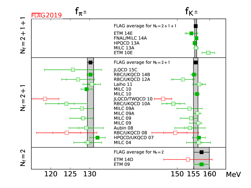
Figure 11: Values of $f_{\pi}$ and $f_{K}$. The black squares and grey bands indicate our estimates (84) and (85).

5 Low-energy constants

Authors: S. Dürr, H. Fukaya, U. M. Heller

In the study of the quark-mass dependence of QCD observables calculated on the lattice, it is common practice to invoke chiral perturbation theory ($\chi$PT). For a given quantity this framework predicts the nonanalytic quark-mass dependence and it provides symmetry relations among different observables. These relations are best expressed with the help of a set of linearly independent and universal (i.e., process-independent) low-energy constants (LECs), which first appear as coefficients of the polynomial terms (in $m_{q}$ or $M_{\pi}^{2}$) in different observables. When numerical simulations are done at heavier than physical (light) quark masses, $\chi$PT is usually invoked in the extrapolation to physical quark masses.

5.1 Chiral perturbation theory

$\chi$PT is an effective field theory approach to the low-energy properties of QCD based on the spontaneous breaking of chiral symmetry, $SU(N_{f})_{L}\times SU(N_{f})_{R}\to SU(N_{f})_{L+R}$, and its soft explicit breaking by quark-mass terms. In its original implementation, in infinite volume, it is an expansion in $m_{q}$ and $p^{2}$ with power counting $M_{\pi}^{2}\sim m_{q}\sim p^{2}$.

If one expands around the $SU(2)$ chiral limit, there appear two LECs at order $p^{2}$ in the chiral effective Lagrangian,

$$F\equiv F_{\pi}\,\rule[-8.5359pt]{0.28436pt}{19.91684pt}_{\;m_{u},m_{d}\rightarrow 0}\quad\mbox{and}\qquad B\equiv\frac{\Sigma}{F^{2}}\;,\quad\mbox{where}\quad\Sigma\equiv-\langle\bar{u}u\rangle\,{\hbox{$\left|\vbox to0.0pt{}\right.\n@space$}}_{\;m_{u},m_{d}\rightarrow 0}\;,$$ (86)

and seven at order $p^{4}$, indicated by $\bar{\ell}_{i}$ with $i=1,\ldots,7$. In the analysis of the $SU(3)$ chiral limit there are also just two LECs at order $p^{2}$,

$$F_{0}\equiv F_{\pi}\,\rule[-8.5359pt]{0.28436pt}{19.91684pt}_{\;m_{u},m_{d},m_{s}\rightarrow 0}\quad\mbox{and}\qquad B_{0}\equiv\frac{\Sigma_{0}}{F_{0}^{2}}\;,\quad\mbox{where}\quad\Sigma_{0}\equiv-\langle\bar{u}u\rangle\,{\hbox{$\left|\vbox to0.0pt{}\right.\n@space$}}_{\;m_{u},m_{d},m_{s}\rightarrow 0}\;,$$ (87)

but ten at order $p^{4}$, indicated by the capital letter $L_{i}(\mu)$ with $i=1,\ldots,10$. These constants are independent of the quark masses, but they become scale dependent after renormalization (sometimes a superscript $r$ is added). The $SU(2)$ constants $\bar{\ell}_{i}$ are scale independent, since they are defined at scale $\mu=M_{\pi,\mathrm{phys}}$ (as indicated by the bar). For the precise definition of these constants and their scale dependence we refer the reader to Refs. [Gasser:1983yg, Gasser:1984gg].

5.1.1 Patterns of chiral symmetry breaking

If the box size is finite but large compared to the Compton wavelength of the pion, $L\gg 1/M_{\pi}$, the power counting generalizes to $m_{q}\sim p^{2}\sim 1/L^{2}$, as one would assume based on the fact that $p_{\mathrm{min}}=2\pi/L$ is the minimum momentum in a finite box with periodic boundary conditions in the spatial directions. This is the so-called $p$-regime of $\chi$PT. It coincides with the setting that is used for standard phenomenologically oriented lattice-QCD computations, and we shall consider the $p$-regime the default in the following. However, if the pion mass is so small that the box-length $L$ is no longer large compared to the Compton wavelength that the pion would have, at the given $m_{q}$, in infinite volume, then the chiral series must be reordered. Such finite-volume versions of $\chi$PT with correspondingly adjusted power counting schemes, referred to as $\epsilon$- and $\delta$-regime, are described in Secs. 5.1.6 and 5.1.7, respectively.

Lattice calculations can be used to test if chiral symmetry is indeed spontaneously broken along the path $SU(N_{f})_{L}\times SU(N_{f})_{R}\to SU(N_{f})_{L+R}$ by measuring nonzero chiral condensates and by verifying the validity of the GMOR relation $M_{\pi}^{2}\propto m_{q}$ close to the chiral limit. If the chiral extrapolation of quantities calculated on the lattice is made with the help of fits to their $\chi$PT forms, apart from determining the observable at the physical value of the quark masses, one also obtains the relevant LECs. This is an important by-product for two reasons:

1. All LECs up to order $p^{4}$ (with the exception of $B$ and $B_{0}$, since only the product of these times the quark masses can be estimated from phenomenology) have either been determined by comparison to experiment or estimated theoretically, e.g., in large-$N_{c}$ QCD. A lattice determination of the better known LECs thus provides a test of the $\chi$PT approach.

2. The less well-known LECs are those which describe the quark-mass dependence of observables—these cannot be determined from experiment, and therefore the lattice, where quark masses can be varied, provides unique quantitative information. This information is essential for improving phenomenological $\chi$PT predictions in which these LECs play a role.

We stress that this program is based on the nonobvious assumption that $\chi$PT is valid in the region of masses and momenta used in the lattice simulations under consideration, something that can and should be checked. With the ability to create data at multiple values of the light-quark masses, lattice QCD offers the possibility to check the convergence of $\chi$PT. Lattice data may be used to verify that higher order contributions, for small enough quark masses, become increasingly unimportant. In the end one wants to compare lattice and phenomenological determinations of LECs, much in the spirit of Ref. [Bijnens:2014lea]. An overview of many of the conceptual issues involved in matching lattice data to an effective field theory framework like $\chi$PT is given in Refs. [Sharpe:2006pu, Golterman:2009kw, Bernard:2015wda].

The fact that, at large volume, the finite-size effects, which occur if a system undergoes spontaneous symmetry breakdown, are controlled by the Nambu-Goldstone modes, was first noted in solid state physics, in connection with magnetic systems [Fisher:1985zz, Brezin:1985xx]. As pointed out in Ref. [Gasser:1986vb] in the context of QCD, the thermal properties of such systems can be studied in a systematic and model-independent manner by means of the corresponding effective field theory, provided the temperature is low enough. While finite volumes are not of physical interest in particle physics, lattice simulations are necessarily carried out in a finite box. As shown in Refs. [Gasser:1987ah, Gasser:1987zq, Hasenfratz:1989pk], the ensuing finite-size effects can be studied on the basis of the effective theory—$\chi$PT in the case of QCD—provided the simulation is close enough to the continuum limit, the volume is sufficiently large and the explicit breaking of chiral symmetry generated by the quark masses is sufficiently small. Indeed, $\chi$PT represents a useful tool for the analysis of the finite-size effects in lattice simulations.

In the remainder of this subsection we collect the relevant $\chi$PT formulae that will be used in the two following subsections to extract $SU(2)$ and $SU(3)$ LECs from lattice data.

5.1.2 Quark-mass dependence of pseudoscalar masses and decay constants

A. $SU(2)$ formulae

The expansions of $M_{\pi}^{2}$ and $F_{\pi}$ in powers of the quark mass are known to next-to-next-to-leading order (NNLO) in the $SU(2)$ chiral effective theory. In the isospin limit, $m_{u}=m_{d}=m$, the explicit expressions may be written in the form [Colangelo:2001df]

$$M_{\pi}^{2} = M^{2}\left\{1-\frac{1}{2}x\ln\frac{\Lambda_{3}^{2}}{M^{2}}+\frac{17}{8}x^{2}\left(\ln\frac{\Lambda_{M}^{2}}{M^{2}}\right)^{2}+x^{2}k_{M}+\mathcal{O}(x^{3})\right\},$$ (88)

$$F_{\pi} = F\left\{1+x\ln\frac{\Lambda_{4}^{2}}{M^{2}}-\frac{5}{4}x^{2}\left(\ln\frac{\Lambda_{F}^{2}}{M^{2}}\right)^{2}+x^{2}k_{F}+\mathcal{O}(x^{3})\right\}.$$

Here the expansion parameter is given by

$$x=\frac{M^{2}}{(4\pi F)^{2}},\;\;\;\;\;\;\;\;\;\;M^{2}=2Bm=\frac{2\Sigma m}{F^{2}},$$ (89)

but there is another option as discussed below. The scales $\Lambda_{3},\Lambda_{4}$ are related to the effective coupling constants $\bar{\ell}_{3},\bar{\ell}_{4}$ of the chiral Lagrangian at scale $\mu=M_{\pi,\mathrm{phys}}$ by

$$\bar{\ell}_{n}=\ln\frac{\Lambda_{n}^{2}}{M_{\pi,\mathrm{phys}}^{2}},\;\;\;\;\;\;\;\;\;\;\;n=1,...,7.$$ (90)

Note that in Eq. (88) the logarithms are evaluated at $M^{2}$, not at $M_{\pi}^{2}$. The coupling constants $k_{M},k_{F}$ in Eq. (88) are mass-independent. The scales of the squared logarithms can be expressed in terms of the $\mathcal{O}(p^{4})$ coupling constants as

$$\ln\frac{\Lambda_{M}^{2}}{M^{2}} = \frac{1}{51}\left(28\ln\frac{\Lambda_{1}^{2}}{M^{2}}+32\ln\frac{\Lambda_{2}^{2}}{M^{2}}-9\ln\frac{\Lambda_{3}^{2}}{M^{2}}+49\right),$$ (91)

$$\ln\frac{\Lambda_{F}^{2}}{M^{2}} = \frac{1}{30}\left(14\ln\frac{\Lambda_{1}^{2}}{M^{2}}+16\ln\frac{\Lambda_{2}^{2}}{M^{2}}+6\ln\frac{\Lambda_{3}^{2}}{M^{2}}-6\ln\frac{\Lambda_{4}^{2}}{M^{2}}+23\right).$$

Hence by analysing the quark-mass dependence of $M_{\pi}^{2}$ and $F_{\pi}$ with Eq. (88), possibly truncated at NLO, one can determine the $\mathcal{O}(p^{2})$ LECs $B$ and $F$, as well as the $\mathcal{O}(p^{4})$ LECs $\bar{\ell}_{3}$ and $\bar{\ell}_{4}$. The quark condensate in the chiral limit is given by $\Sigma=F^{2}B$. With precise enough data at several small enough pion masses, one could in principle also determine $\Lambda_{M}$, $\Lambda_{F}$ and $k_{M}$, $k_{F}$. To date this is not yet possible. The results for the LO and NLO constants will be presented in Sec. 5.2.

Alternatively, one can invert Eq. (88) and express $M^{2}$ and $F$ as an expansion in

$$\xi\equiv\frac{M_{\pi}^{2}}{16\pi^{2}F_{\pi}^{2}}\;\;,$$ (92)

and the corresponding expressions then take the form

$$M^{2} = M_{\pi}^{2}\,\left\{1+\frac{1}{2}\,\xi\,\ln\frac{\Lambda_{3}^{2}}{M_{\pi}^{2}}-\frac{5}{8}\,\xi^{2}\left(\!\ln\frac{\Omega_{M}^{2}}{M_{\pi}^{2}}\!\right)^{2}+\xi^{2}c_{\scriptscriptstyle M}+\mathcal{O}(\xi^{3})\right\}\,,$$ (93)

$$F = F_{\pi}\,\left\{1-\xi\,\ln\frac{\Lambda_{4}^{2}}{M_{\pi}^{2}}-\frac{1}{4}\,\xi^{2}\left(\!\ln\frac{\Omega_{F}^{2}}{M_{\pi}^{2}}\!\right)^{2}+\xi^{2}c_{\scriptscriptstyle F}+\mathcal{O}(\xi^{3})\right\}\,.$$

The scales of the quadratic logarithms are determined by $\Lambda_{1},\ldots,\Lambda_{4}$ through

$$\ln\frac{\Omega_{M}^{2}}{M_{\pi}^{2}} = \frac{1}{15}\left(28\,\ln\frac{\Lambda_{1}^{2}}{M_{\pi}^{2}}+32\,\ln\frac{\Lambda_{2}^{2}}{M_{\pi}^{2}}-33\,\ln\frac{\Lambda_{3}^{2}}{M_{\pi}^{2}}-12\,\ln\frac{\Lambda_{4}^{2}}{M_{\pi}^{2}}+52\right)\,,$$ (94)

$$\ln\frac{\Omega_{F}^{2}}{M_{\pi}^{2}} = \frac{1}{3}\,\left(-7\,\ln\frac{\Lambda_{1}^{2}}{M_{\pi}^{2}}-8\,\ln\frac{\Lambda_{2}^{2}}{M_{\pi}^{2}}+18\,\ln\frac{\Lambda_{4}^{2}}{M_{\pi}^{2}}-\frac{29}{2}\right)\,.$$

In practice, many results are expressed in terms of the LO constants $F$ and $\Sigma$ and the NLO constants $\bar{\ell}_{i}$. The LO constants relate to the LO constants used above through $B=\Sigma/F^{2}$. At the NLO the relation is a bit more involved, since the $\bar{\ell}_{i}$ bear the notion of the physical pion mass, see (90). For instance, Eqs. (93) may be rewritten as

$$M^{2} = M_{\pi}^{2}\,\left\{1+\frac{1}{2}\,\xi\,\bar{\ell}_{3}+\frac{1}{2}\,\xi\ln\frac{M_{\pi,\mathrm{phys}}^{2}}{M_{\pi}^{2}}-\frac{5}{8}\,\xi^{2}\left(\!\ln\frac{\Omega_{M}^{2}}{M_{\pi}^{2}}\!\right)^{2}+\xi^{2}c_{\scriptscriptstyle M}+\mathcal{O}(\xi^{3})\right\}\,,$$ (95)

$$F = F_{\pi}\,\left\{1-\xi\,\bar{\ell}_{4}-\xi\,\ln\frac{M_{\pi,\mathrm{phys}}^{2}}{M_{\pi}^{2}}-\frac{1}{4}\,\xi^{2}\left(\!\ln\frac{\Omega_{F}^{2}}{M_{\pi}^{2}}\!\right)^{2}+\xi^{2}c_{\scriptscriptstyle F}+\mathcal{O}(\xi^{3})\right\}\,,$$

and this implies that fitting some lattice data (say at a single lattice spacing $a$) with Eq. (95) requires some a-priori knowledge of the lattice spacing. On the other hand, doing the same job with Eq. (93) yields the scales $a\Lambda_{3},a\Lambda_{4}$ in lattice units (which may be converted to $\bar{\ell}_{3},\bar{\ell}_{4}$ at a later stage of the analysis when the scale is known more precisely).

B. $SU(3)$ formulae

While the formulae for the pseudoscalar masses and decay constants are known to NNLO for $SU(3)$ as well [Amoros:1999dp], they are rather complicated and we restrict ourselves here to next-to-leading order (NLO). In the isospin limit, the relevant $SU(3)$ formulae take the form [Gasser:1984gg]

$$M_{\pi}^{2}\!\! \!\!\stackrel{{\scriptstyle\rule[-2.84544pt]{0.0pt}{0.0pt}\mbox{\tiny NLO}}}{{=}}\!\! \!\!2B_{0}m_{ud}{\hbox{$\left\{\vbox to0.0pt{}\right.\n@space$}}1+\mu_{\pi}-\frac{1}{3}\mu_{\eta}+\frac{B_{0}}{F_{0}^{2}}{\hbox{$\left[\vbox to0.0pt{}\right.\n@space$}}16m_{ud}(2L_{8}\!-\!L_{5})+16(m_{s}\!+\!2m_{ud})(2L_{6}\!-\!L_{4}){\hbox{$\left]\vbox to0.0pt{}\right.\n@space$}}{\hbox{$\left\}\vbox to0.0pt{}\right.\n@space$}}\;,$$

$$M_{\!K}^{2}\!\! \!\!\stackrel{{\scriptstyle\rule[-2.84544pt]{0.0pt}{0.0pt}\mbox{\tiny NLO}}}{{=}}\!\! \!\!B_{0}(m_{s}\!\!+\!m_{ud}){\hbox{$\left\{\vbox to0.0pt{}\right.\n@space$}}1\!+\!\frac{2}{3}\mu_{\eta}\!+\!\frac{B_{0}}{F_{0}^{2}}{\hbox{$\left[\vbox to0.0pt{}\right.\n@space$}}8(m_{s}\!\!+\!m_{ud})(2L_{8}\!-\!L_{5})\!+\!16(m_{s}\!\!+\!2m_{ud})(2L_{6}\!-\!L_{4}){\hbox{$\left]\vbox to0.0pt{}\right.\n@space$}}{\hbox{$\left\}\vbox to0.0pt{}\right.\n@space$}}\;,\quad$$

$$F_{\pi}\!\! \!\!\stackrel{{\scriptstyle\rule[-2.84544pt]{0.0pt}{0.0pt}\mbox{\tiny NLO}}}{{=}}\!\! \!\!F_{0}{\hbox{$\left\{\vbox to0.0pt{}\right.\n@space$}}1-2\mu_{\pi}-\mu_{K}+\frac{B_{0}}{F_{0}^{2}}{\hbox{$\left[\vbox to0.0pt{}\right.\n@space$}}8m_{ud}L_{5}+8(m_{s}\!+\!2m_{ud})L_{4}{\hbox{$\left]\vbox to0.0pt{}\right.\n@space$}}{\hbox{$\left\}\vbox to0.0pt{}\right.\n@space$}}\;,$$ (96)

$$F_{K}\!\! \!\!\stackrel{{\scriptstyle\rule[-2.84544pt]{0.0pt}{0.0pt}\mbox{\tiny NLO}}}{{=}}\!\! \!\!F_{0}{\hbox{$\left\{\vbox to0.0pt{}\right.\n@space$}}1-\frac{3}{4}\mu_{\pi}-\frac{3}{2}\mu_{K}-\frac{3}{4}\mu_{\eta}+\frac{B_{0}}{F_{0}^{2}}{\hbox{$\left[\vbox to0.0pt{}\right.\n@space$}}4(m_{s}\!+\!m_{ud})L_{5}+8(m_{s}\!+\!2m_{ud})L_{4}{\hbox{$\left]\vbox to0.0pt{}\right.\n@space$}}{\hbox{$\left\}\vbox to0.0pt{}\right.\n@space$}}\;,$$

where $m_{ud}$ is the joint up/down quark mass in the simulation [which may be taken different from the average light-quark mass $\frac{1}{2}(m_{u}^{\mathrm{phys}}+m_{d}^{\mathrm{phys}})$ in the real world]. And $B_{0}=\Sigma_{0}/F_{0}^{2}$, $F_{0}$ denote the condensate parameter and the pseudoscalar decay constant in the $SU(3)$ chiral limit, respectively. In addition, we use the notation

$$\mu_{P}=\frac{M_{P}^{2}}{32\pi^{2}F_{0}^{2}}\ln\!{\hbox{$\left(\vbox to0.0pt{}\right.\n@space$}}\frac{M_{P}^{2}}{\mu^{2}}{\hbox{$\left)\vbox to0.0pt{}\right.\n@space$}}\;.$$ (97)

At the order of the chiral expansion used in these formulae, the quantities $\mu_{\pi}$, $\mu_{K}$, $\mu_{\eta}$ can equally well be evaluated with the leading-order expressions for the masses,

$$M_{\pi}^{2}\stackrel{{\scriptstyle\rule[-2.84544pt]{0.0pt}{0.0pt}\mbox{\tiny LO}}}{{=}}2B_{0}\,m_{ud}\;,\quad M_{K}^{2}\stackrel{{\scriptstyle\rule[-2.84544pt]{0.0pt}{0.0pt}\mbox{\tiny LO}}}{{=}}B_{0}(m_{s}\!+\!m_{ud})\;,\quad M_{\eta}^{2}\stackrel{{\scriptstyle\rule[-2.84544pt]{0.0pt}{0.0pt}\mbox{\tiny LO}}}{{=}}\mbox{$\frac{2}{3}$}B_{0}(2m_{s}\!+\!m_{ud})\;.$$ (98)

Throughout, $L_{i}$ denotes the renormalized low-energy constant/coupling (LEC) at scale $\mu$, and we adopt the convention that is standard in phenomenology, $\mu=M_{\rho}=770\,\mathrm{MeV}$. The normalization used for the decay constants is specified in footnote 24.

5.1.3 Pion form factors and charge radii

The scalar and vector form factors of the pion are defined by the matrix elements

$$\langle\pi^{i}(p_{2})|\,\bar{q}\,q\,|\pi^{k}(p_{1})\rangle \!\!\!= \!\!\!\delta^{ik}F_{S}^{\pi}(t)\,,$$ (99)

$$\langle\pi^{i}(p_{2})|\,\bar{q}\,\mbox{$\frac{1}{2}$}\tau^{j}\gamma^{\mu}q\,|\pi^{k}(p_{1})\rangle \!\!\!= \!\!\!\mathrm{i}\,\epsilon^{ijk}(p_{1}^{\mu}+p_{2}^{\mu})F_{V}^{\pi}(t)\,,$$

where the operators contain only the lightest two quark flavours, i.e., $\tau^{1}$, $\tau^{2}$, $\tau^{3}$ are the Pauli matrices, and $t\equiv(p_{1}-p_{2})^{2}$ denotes the momentum transfer.

The vector form factor has been measured by several experiments for time-like as well as for space-like values of $t$. The scalar form factor is not directly measurable, but it can be evaluated theoretically from data on the $\pi\pi$ and $\pi K$ phase shifts [Donoghue:1990xh] by means of analyticity and unitarity, i.e., in a model-independent way. Lattice calculations can be compared with data or model-independent theoretical evaluations at any given value of $t$. At present, however, most lattice studies concentrate on the region close to $t=0$ and on the evaluation of the slope and curvature, which are defined as

$$F^{\pi}_{V}(t) = 1+\mbox{$\frac{1}{6}$}\langle r^{2}\rangle^{\pi}_{V}t+c_{V}\hskip 0.71114ptt^{2}+\ldots\;\,,$$ (100)

$$F^{\pi}_{S}(t) = F^{\pi}_{S}(0)\left[1+\mbox{$\frac{1}{6}$}\langle r^{2}\rangle^{\pi}_{S}t+c_{S}\,t^{2}+\ldots\right]\;\;.$$

The slopes are related to the mean-square vector and scalar radii, which are the quantities on which most experiments and lattice calculations concentrate.

In $\chi$PT, the form factors are known at NNLO for $SU(2)$ [Bijnens:1998fm]. The corresponding formulae are available in fully analytical form and are compact enough that they can be used for the chiral extrapolation of the data (as done, for example, in Refs. [Frezzotti:2008dr, Kaneko:2008kx]). The expressions for the scalar and vector radii and for the $c_{S,V}$ coefficients at 2-loop level in $SU(2)$ terminology read

$$\langle r^{2}\rangle^{\pi}_{S} = \frac{1}{(4\pi F_{\pi})^{2}}\left\{6\ln\frac{\Lambda_{4}^{2}}{M_{\pi}^{2}}-\frac{13}{2}-\frac{29}{3}\,\xi\left(\!\ln\frac{\Omega_{r_{S}}^{2}}{M_{\pi}^{2}}\!\right)^{2}+6\xi\,k_{r_{S}}+\mathcal{O}(\xi^{2})\right\}\,,$$

$$\langle r^{2}\rangle^{\pi}_{V} = \frac{1}{(4\pi F_{\pi})^{2}}\left\{\ln\frac{\Lambda_{6}^{2}}{M_{\pi}^{2}}-1+2\,\xi\left(\!\ln\frac{\Omega_{r_{V}}^{2}}{M_{\pi}^{2}}\!\right)^{2}+6\xi\,k_{r_{V}}+\mathcal{O}(\xi^{2})\right\}\,,$$ (101)

$$c_{S} = \frac{1}{(4\pi F_{\pi}M_{\pi})^{2}}\left\{\frac{19}{120}+\xi\left[\frac{43}{36}\left(\!\ln\frac{\Omega_{c_{S}}^{2}}{M_{\pi}^{2}}\!\right)^{2}+k_{c_{S}}\right]\right\}\,,$$

$$c_{V} = \frac{1}{(4\pi F_{\pi}M_{\pi})^{2}}\left\{\frac{1}{60}+\xi\left[\frac{1}{72}\left(\!\ln\frac{\Omega_{c_{V}}^{2}}{M_{\pi}^{2}}\!\right)^{2}+k_{c_{V}}\right]\right\}\,,$$

where

$$\ln\frac{\Omega_{r_{S}}^{2}}{M_{\pi}^{2}} = \frac{1}{29}\,\left(31\,\ln\frac{\Lambda_{1}^{2}}{M_{\pi}^{2}}+34\,\ln\frac{\Lambda_{2}^{2}}{M_{\pi}^{2}}-36\,\ln\frac{\Lambda_{4}^{2}}{M_{\pi}^{2}}+\frac{145}{24}\right)\,,$$

$$\ln\frac{\Omega_{r_{V}}^{2}}{M_{\pi}^{2}} = \frac{1}{2}\,\left(\ln\frac{\Lambda_{1}^{2}}{M_{\pi}^{2}}-\ln\frac{\Lambda_{2}^{2}}{M_{\pi}^{2}}+\ln\frac{\Lambda_{4}^{2}}{M_{\pi}^{2}}+\ln\frac{\Lambda_{6}^{2}}{M_{\pi}^{2}}-\frac{31}{12}\right)\,,$$ (102)

$$\ln\frac{\Omega_{c_{S}}^{2}}{M_{\pi}^{2}} = \frac{43}{63}\,\left(11\,\ln\frac{\Lambda_{1}^{2}}{M_{\pi}^{2}}+14\,\ln\frac{\Lambda_{2}^{2}}{M_{\pi}^{2}}+18\,\ln\frac{\Lambda_{4}^{2}}{M_{\pi}^{2}}-\frac{6041}{120}\right)\,,$$

$$\ln\frac{\Omega_{c_{V}}^{2}}{M_{\pi}^{2}} = \frac{1}{72}\,\left(2\ln\frac{\Lambda_{1}^{2}}{M_{\pi}^{2}}-2\ln\frac{\Lambda_{2}^{2}}{M_{\pi}^{2}}-\ln\frac{\Lambda_{6}^{2}}{M_{\pi}^{2}}-\frac{26}{30}\right)\,,$$

and $k_{r_{S}},k_{r_{V}}$ and $k_{c_{S}},k_{c_{V}}$ are independent of the quark masses. Their expression in terms of the $\ell_{i}$ and of the $\mathcal{O}(p^{6})$ constants $c_{M},c_{F}$ is known but will not be reproduced here.

The $SU(3)$ formula for the slope of the pion vector form factor reads, to NLO [Gasser:1984ux],

$$\langle r^{2}\rangle_{V}^{\pi}\;\stackrel{{\scriptstyle\rule[-2.84544pt]{0.0pt}{0.0pt}\mbox{\tiny NLO}}}{{=}}\;-\frac{1}{32\pi^{2}F_{0}^{2}}{\hbox{$\left\{\vbox to0.0pt{}\right.\n@space$}}3+2\ln\frac{M_{\pi}^{2}}{\mu^{2}}+\ln\frac{M_{K}^{2}}{\mu^{2}}{\hbox{$\left\}\vbox to0.0pt{}\right.\n@space$}}+\frac{12L_{9}}{F_{0}^{2}}\;,$$ (103)

while the expression $\langle r^{2}\rangle_{S}^{\mathrm{oct}}$ for the octet part of the scalar radius does not contain any NLO low-energy constant at 1-loop order [Gasser:1984ux]—contrary to the situation in $SU(2)$, see Eq. (101).

The difference between the quark-line connected and the full (i.e., containing the connected and the disconnected pieces) scalar pion form factor has been investigated by means of $\chi$PT in Ref. [Juttner:2011ur]. It is expected that the technique used can be applied to a large class of observables relevant in QCD phenomenology.

As a point of practical interest let us remark that there are no finite-volume correction formulae for the mean-square radii $\langle r^{2}\rangle_{V,S}$ and the curvatures $c_{V,S}$. The lattice data for $F_{V,S}(t)$ need to be corrected, point by point in $t$, for finite-volume effects. In fact, if a given $\sqrt{t}$ is realized through several inequivalent $p_{1}\!-\!p_{2}$ combinations, the level of agreement after the correction has been applied is indicative of how well higher-order and finite-volume effects are under control.

5.1.4 Goldstone boson scattering in a finite volume

The scattering of pseudoscalar octet mesons off each other (mostly $\pi$-$\pi$ and $\pi$-$K$ scattering) is a useful approach to determine $\chi$PT low-energy constants [Weinberg:1966kf, Gasser:1983kx, Bijnens:1995yn, Colangelo:2001df, Nebreda:2010wv]. This statement holds true both in experiment and on the lattice. We would like to point out that the main difference between these approaches is not so much the discretization of space-time, but rather the Minkowskian versus Euclidean setup.

In infinite-volume Minkowski space-time, 4-point Green’s functions can be evaluated (e.g., in experiment) for a continuous range of (on-shell) momenta, as captured, for instance, by the Mandelstam variable $s$. For a given isospin channel $I=0$ or $I=2$ the $\pi$-$\pi$ scattering phase shift $\delta^{I}(s)$ can be determined for a variety of $s$ values, and by matching to $\chi$PT some low-energy constants can be determined (see below). In infinite-volume Euclidean space-time, such 4-point Green’s functions can only be evaluated at kinematic thresholds; this is the content of the so-called Maiani-Testa theorem [Maiani:1990ca]. However, in the Euclidean case, the finite volume comes to our rescue, as first pointed out by Lüscher [Luscher:1985dn, Luscher:1986pf, Luscher:1990ux, Luscher:1991cf]. By comparing the energy of the (interacting) two-pion system in a box with finite spatial extent $L$ to twice the energy of a pion (with identical bare parameters) in infinite volume information on the scattering length can be obtained. In particular in the (somewhat idealized) situation where one can “scan” through a narrowly spaced set of box-sizes $L$ such information can be reconstructed in an efficient way.

We begin with a brief summary of the relevant formulae from $\chi$PT in $SU(2)$ terminology. In the $x$-expansion the formulae for $a_{\ell}^{I}$ with $\ell=0$ and $I=0,2$ are found in Ref. [Gasser:1983yg]

$$a_{0}^{0}M_{\pi} = +\frac{7M^{2}}{32\pi F^{2}}{\hbox{$\left\{\vbox to0.0pt{}\right.\n@space$}}1+\frac{5M^{2}}{84\pi^{2}F^{2}}{\hbox{$\left[\vbox to0.0pt{}\right.\n@space$}}\bar{\ell}_{1}+2\bar{\ell}_{2}-\frac{9}{10}\bar{\ell}_{3}+\frac{21}{8}{\hbox{$\left]\vbox to0.0pt{}\right.\n@space$}}+\mathcal{O}(x^{2}){\hbox{$\left\}\vbox to0.0pt{}\right.\n@space$}}\;,$$ (104)

$$a_{0}^{2}M_{\pi} = -\frac{M^{2}}{16\pi F^{2}}{\hbox{$\left\{\vbox to0.0pt{}\right.\n@space$}}1-\frac{M^{2}}{12\pi^{2}F^{2}}{\hbox{$\left[\vbox to0.0pt{}\right.\n@space$}}\bar{\ell}_{1}+2\bar{\ell}_{2}+\frac{3}{8}{\hbox{$\left]\vbox to0.0pt{}\right.\n@space$}}+\mathcal{O}(x^{2}){\hbox{$\left\}\vbox to0.0pt{}\right.\n@space$}}\;,$$ (105)

where we deviate from the $\chi$PT habit of absorbing a factor $-M_{\pi}$ into the scattering length (relative to the convention used in quantum mechanics), since we include just a minus sign but not the factor $M_{\pi}$. Hence, our $a_{\ell}^{I}$ have the dimension of a length so that all quark- or pion-mass dependence is explicit (as is most convenient for the lattice community). But the sign convention is the one of the chiral community (where $a_{\ell}^{I}M_{\pi}>0$ means attraction and $a_{\ell}^{I}M_{\pi}<0$ means repulsion).

An important difference between the two scattering lengths is evident already at tree-level. The isospin-0 $S$-wave scattering length (104) is large and positive, while the isospin-2 counterpart (105) is by a factor $\sim 3.5$ smaller (in absolute magnitude) and negative. Hence, in the channel with $I=0$ the interaction is attractive, while in the channel with $I=2$ the interaction is repulsive and significantly weaker. In this convention experimental results, evaluated with the unitarity constraint genuine to any local quantum field theory, read $a_{0}^{0}M_{\pi}=0.2198(46)_{\mathrm{stat}}(16)_{\mathrm{syst}}(64)_{\mathrm{theo}}$ and $a_{0}^{2}M_{\pi}=-0.0445(11)_{\mathrm{stat}}(4)_{\mathrm{syst}}(8)_{\mathrm{theo}}$ [Roy:1971tc, Ananthanarayan:2000ht, Colangelo:2001df, Caprini:2011ky]. The ratio between the two (absolute) central values is larger than $3.5$, and this suggests that NLO contributions to $a_{0}^{0}$ might be more relevant than NLO contributions to $a_{0}^{2}$.

By means of $M^{2}/(4\pi F)^{2}=M_{\pi}^{2}/(4\pi F_{\pi})^{2}\{1+\frac{1}{2}\xi\ln(\Lambda_{3}^{2}/M_{\pi}^{2})+2\xi\ln(\Lambda_{4}^{2}/M_{\pi}^{2})+\mathcal{O}(\xi^{2})\}$ or equivalently through $M^{2}/(4\pi F)^{2}=M_{\pi}^{2}/(4\pi F_{\pi})^{2}\{1+\frac{1}{2}\xi\bar{\ell}_{3}+2\xi\bar{\ell}_{4}+\mathcal{O}(\xi^{2})\}$ Eqs. (104, 105) may be brought into the form

$$a_{0}^{0}M_{\pi} = +\frac{7M_{\pi}^{2}}{32\pi F_{\pi}^{2}}{\hbox{$\left\{\vbox to0.0pt{}\right.\n@space$}}1+\xi\frac{1}{2}\bar{\ell}_{3}+\xi 2\bar{\ell}_{4}+\xi{\hbox{$\left[\vbox to0.0pt{}\right.\n@space$}}\frac{20}{21}\bar{\ell}_{1}+\frac{40}{21}\bar{\ell}_{2}-\frac{18}{21}\bar{\ell}_{3}+\frac{5}{2}{\hbox{$\left]\vbox to0.0pt{}\right.\n@space$}}+\mathcal{O}(\xi^{2}){\hbox{$\left\}\vbox to0.0pt{}\right.\n@space$}}\;,$$ (106)

$$a_{0}^{2}M_{\pi} = -\frac{M_{\pi}^{2}}{16\pi F_{\pi}^{2}}{\hbox{$\left\{\vbox to0.0pt{}\right.\n@space$}}1+\xi\frac{1}{2}\bar{\ell}_{3}+\xi 2\bar{\ell}_{4}-\xi{\hbox{$\left[\vbox to0.0pt{}\right.\n@space$}}\frac{4}{3}\bar{\ell}_{1}+\frac{8}{3}\bar{\ell}_{2}+\frac{1}{2}{\hbox{$\left]\vbox to0.0pt{}\right.\n@space$}}+\mathcal{O}(\xi^{2}){\hbox{$\left\}\vbox to0.0pt{}\right.\n@space$}}\;.$$ (107)

Finally, this expression can be summarized as

$$a_{0}^{0}M_{\pi} = +\frac{7M_{\pi}^{2}}{32\pi F_{\pi}^{2}}{\hbox{$\left\{\vbox to0.0pt{}\right.\n@space$}}1+\frac{9M_{\pi}^{2}}{32\pi^{2}F_{\pi}^{2}}\ln\frac{(\lambda_{0}^{0})^{2}}{M_{\pi}^{2}}+\mathcal{O}(\xi^{2}){\hbox{$\left\}\vbox to0.0pt{}\right.\n@space$}}\;,$$ (108)

$$a_{0}^{2}M_{\pi} = -\frac{M_{\pi}^{2}}{16\pi F_{\pi}^{2}}{\hbox{$\left\{\vbox to0.0pt{}\right.\n@space$}}1-\frac{3M_{\pi}^{2}}{32\pi^{2}F_{\pi}^{2}}\ln\frac{(\lambda_{0}^{2})^{2}}{M_{\pi}^{2}}+\mathcal{O}(\xi^{2}){\hbox{$\left\}\vbox to0.0pt{}\right.\n@space$}}\;,$$ (109)

with the abbreviations

$$\frac{9}{2}\ln\frac{(\lambda_{0}^{0})^{2}}{M_{\pi,\mathrm{phys}}^{2}} = \frac{20}{21}\bar{\ell}_{1}+\frac{40}{21}\bar{\ell}_{2}-\frac{5}{14}\bar{\ell}_{3}+2\bar{\ell}_{4}+\frac{5}{2}\;,$$ (110)

$$\frac{3}{2}\ln\frac{(\lambda_{0}^{2})^{2}}{M_{\pi,\mathrm{phys}}^{2}} = \frac{4}{3}\bar{\ell}_{1}+\frac{8}{3}\bar{\ell}_{2}-\frac{1}{2}\bar{\ell}_{3}-2\bar{\ell}_{4}+\frac{1}{2}\;,$$ (111)

where $\lambda_{\ell}^{I}$ with $\ell=0$ and $I=0,2$ are scales like the $\Lambda_{i}$ in $\bar{\ell}_{i}=\ln(\Lambda_{i}^{2}/M_{\pi,\mathrm{phys}}^{2})$ for $i\in\{1,2,3,4\}$ (albeit they are not independent from the latter). Here we made use of the fact that $M_{\pi}^{2}/M_{\pi,\mathrm{phys}}^{2}=1+\mathcal{O}(\xi)$ and thus $\xi\ln(M_{\pi}^{2}/M_{\pi,\mathrm{phys}}^{2})=\mathcal{O}(\xi^{2})$. In the absence of any knowledge on the $\bar{\ell}_{i}$ one would assume $\lambda_{0}^{0}\simeq\lambda_{0}^{2}$, and with this input Eqs. (108, 109) suggest that the NLO contribution to $|a_{0}^{0}|$ is by a factor $\sim 9$ larger than the NLO contribution to $|a_{0}^{2}|$. The experimental numbers quoted before clearly support this view.

Given that all of this sounds like a complete success story for the determination of the scattering lengths $a_{0}^{0}$ and $a_{0}^{2}$, one may wonder whether lattice QCD is helpful at all. It is, because the “experimental” evaluation of these scattering lengths builds on a constraint between these two quantities that, in turn, is based on a (rather nontrivial) dispersive evaluation of scattering phase shifts [Roy:1971tc, Ananthanarayan:2000ht, Colangelo:2001df, Caprini:2011ky]. Hence, to overcome this possible loophole, an independent lattice determination of $a_{0}^{0}$ and/or $a_{0}^{2}$ is highly welcome.

On the lattice $a_{0}^{2}$ is much easier to determine than $a_{0}^{0}$, since the former quantity does not involve quark-line disconnected contributions. The main upshot of such activities (to be reviewed below) is that the lattice determination of $a_{0}^{2}M_{\pi}$ at the physical mass point is in perfect agreement with the experimental numbers quoted before, thus supporting the view that the scalar condensate is—at least in the $SU(2)$ case—the dominant order parameter, and the original estimate $\bar{\ell}_{3}=2.9\pm 2.4$ is correct (see below). Still, from a lattice perspective it is natural to see a determination of $a_{0}^{0}M_{\pi}$ and/or $a_{0}^{2}M_{\pi}$ as a means to access the specific linear combinations of $\bar{\ell}_{i}$ with $i\in\{1,2,3,4\}$ defined in Eqs. (110, 111).

In passing we note that an alternative version of Eqs. (108, 109) is used in the literature, too. For instance Refs. [Beane:2007xs, Feng:2009ij, Fu:2013ffa, Helmes:2015gla, Liu:2016cba] give their results in the form

$$a_{0}^{0}M_{\pi} = +\frac{7M_{\pi}^{2}}{32\pi F_{\pi}^{2}}{\hbox{$\left\{\vbox to0.0pt{}\right.\n@space$}}1+\frac{M_{\pi}^{2}}{32\pi^{2}F_{\pi}^{2}}{\hbox{$\left[\vbox to0.0pt{}\right.\n@space$}}\ell^{I=0}_{\pi\pi}+5-9\ln\frac{M_{\pi}^{2}}{2F_{\pi}^{2}}{\hbox{$\left]\vbox to0.0pt{}\right.\n@space$}}+\mathcal{O}(\xi^{2}){\hbox{$\left\}\vbox to0.0pt{}\right.\n@space$}}\;,$$ (112)

$$a_{0}^{2}M_{\pi} = -\frac{M_{\pi}^{2}}{16\pi F_{\pi}^{2}}{\hbox{$\left\{\vbox to0.0pt{}\right.\n@space$}}1-\frac{M_{\pi}^{2}}{32\pi^{2}F_{\pi}^{2}}{\hbox{$\left[\vbox to0.0pt{}\right.\n@space$}}\ell^{I=2}_{\pi\pi}+1-3\ln\frac{M_{\pi}^{2}}{2F_{\pi}^{2}}{\hbox{$\left]\vbox to0.0pt{}\right.\n@space$}}+\mathcal{O}(\xi^{2}){\hbox{$\left\}\vbox to0.0pt{}\right.\n@space$}}\;,$$ (113)

where the quantities (used to quote the results of the lattice calculation)

$$\ell^{I=0}_{\pi\pi} = \frac{40}{21}\bar{\ell_{1}}+\frac{80}{21}\bar{\ell_{2}}-\frac{5}{7}\bar{\ell_{3}}+4\bar{\ell_{4}}+9\ln\frac{M_{\pi,\mathrm{phys}}^{2}}{2F^{2}_{\pi,\mathrm{phys}}}\;,$$ (114)

$$\ell^{I=2}_{\pi\pi} = \frac{8}{3}\bar{\ell_{1}}+\frac{16}{3}\bar{\ell_{2}}-\bar{\ell_{3}}-4\bar{\ell_{4}}+3\ln\frac{M_{\pi,\mathrm{phys}}^{2}}{2F^{2}_{\pi,\mathrm{phys}}}\;,$$ (115)

amount to linear combinations of the $\ell_{i}^{\mathrm{ren}}(\mu^{\mathrm{ren}})$ that, due to the explicit logarithms in Eqs. (114, 115), are effectively renormalized at the scale $\mu_{\mathrm{ren}}=f_{\pi,\mathrm{phys}}=\sqrt{2}F_{\pi,\mathrm{phys}}$. Note that in these equations the dependence on the physical pion mass in the logarithms cancels the one that comes from the $\bar{\ell}_{i}$, so that the left-hand-sides bear no knowledge of $M_{\pi,\mathrm{phys}}$. This alternative form is slightly different from Eqs. (108, 109). Exact equality would be reached upon substituting $F_{\pi}^{2}\rightarrow F_{\pi,\mathrm{phys}}^{2}$ in the logarithms of Eqs. (112, 113). Upon expanding $F_{\pi}^{2}/F_{\pi,\mathrm{phys}}^{2}$ and subsequently the logarithm, one realizes that this difference amounts to a term $O(\xi)$ within the square bracket. It thus makes up for a difference at the NNLO, which is beyond the scope of these formulae.

We close by mentioning a few works that elaborate on specific issues in $\pi$-$\pi$ scattering relevant to the lattice. Ref. [Chen:2005ab] does mixed action $\chi$PT for 2 and 2+1 flavors of staggered sea quarks and Ginsparg-Wilson valence quarks, Refs. [Buchoff:2008ve, Aoki:2008gy] work out scattering formulae in Wilson fermion $\chi$PT, and Ref. [Acharya:2017zje] lists connected and disconnected contractions in $\pi$-$\pi$ scattering.

5.1.5 Partially quenched and mixed action formulations

The term “partially quenched QCD” is used in two ways. For heavy quarks ($c,b$ and sometimes $s$) it usually means that these flavours are included in the valence sector, but not into the functional determinant, i.e., the sea sector. For the light quarks ($u,d$ and sometimes $s$) it means that they are present in both the valence and the sea sector of the theory, but with different masses (e.g., a series of valence quark masses is evaluated on an ensemble with fixed sea-quark masses).

The program of extending the standard (unitary) $SU(3)$ theory to the (second version of) “partially quenched QCD” has been completed at the 2-loop (NNLO) level for masses and decay constants [Bijnens:2006jv]. These formulae tend to be complicated, with the consequence that a state-of-the-art analysis with $\mathcal{O}(2000)$ bootstrap samples on $\mathcal{O}(20)$ ensembles with $\mathcal{O}(5)$ masses each [and hence $\mathcal{O}(200\,000)$ different fits] will require significant computational resources. For a summary of recent developments in $\chi$PT relevant to lattice QCD we refer to Ref. [Bijnens:2011tb]. The $SU(2)$ partially quenched formulae can be obtained from the $SU(3)$ ones by “integrating out the strange quark”; this involves a matching of the two theories. At NLO, they can be found in Ref. [Du:2009ih] by setting the lattice artifact terms from the staggered $\chi$PT form to zero.

The theoretical underpinning of how “partial quenching” is to be understood in the (properly extended) chiral framework is given in Ref. [Bernard:2013kwa]. Specifically, for partially quenched QCD with staggered quarks it is shown that a transfer matrix can be constructed that is not Hermitian but bounded, and can thus be used to construct correlation functions in the usual way. The program of calculating all observables in the $p$-regime in finite-volume to two loops, first completed in the unitary theory [Bijnens:2013doa, Bijnens:2014dea], has been carried out for the partially quenched case, too [Bijnens:2015dra].

A further extension of the $\chi$PT framework concerns the lattice effects that arise in partially quenched simulations where sea and valence quarks are implemented with different lattice fermion actions [Bar:2002nr, Bar:2003mh, Bar:2005tu, Chen:2009su, Bae:2010ki, Bailey:2012wb, Bernard:2013eya, Bailey:2015zga]. This extension is usually referred to as “mixed-action $\chi$PT” or “mixed-action partially-quenched $\chi$PT”.

5.1.6 Correlation functions in the $\epsilon$-regime

The finite-size effects encountered in lattice calculations can be used to determine some of the LECs of QCD. In order to illustrate this point, we focus on the two lightest quarks, take the isospin limit $m_{u}=m_{d}=m$ and consider a box of size $L_{s}$ in the three space directions and size $L_{t}$ in the time direction. If $m$ is sent to zero at fixed box size, chiral symmetry is restored, and the zero-momentum mode of the pion field becomes nonperturbative. An intuitive way to understand the regime with $ML<1$ ($L=L_{s}\,\raisebox{-1.72218pt}{\hbox to0.0pt{$\sim$\hss}}\raisebox{1.72218pt}{$<$}\,L_{t}$) starts from considering the pion propagator $G(p)=1/(p^{2}+M^{2})$ in finite volume. For $ML\,\raisebox{-1.72218pt}{\hbox to0.0pt{$\sim$\hss}}\raisebox{1.72218pt}{$>$}\,1$ and $p\sim 1/L$, $G(p)\sim L^{2}$ for small momenta, including $p=0$. But when $M$ becomes of order $1/L^{2}$, $G(0)\propto L^{4}\gg G(p\neq 0)\sim L^{2}$. The $p=0$ mode of the pion field becomes nonperturbative, and the integration over this mode restores chiral symmetry in the limit $m\to 0$.

The pion effective action for the zero-momentum field depends only on the combination $\mu=m\Sigma V$, the symmetry-restoration parameter, where $V=L_{s}^{3}L_{t}$ [Leutwyler:1992yt]. In the $\epsilon$-regime, where $ML\ll 1$ with $L\equiv V^{1/4}$ and hence $m\ll 1/(2BL^{2})$, all other terms in the effective action are sub-dominant in powers of $\epsilon\sim 1/L$. This amounts to a reordering of the chiral expansion, based on $m\sim\epsilon^{4}$ in the $\epsilon$-regime [Leutwyler:1992yt]. In the $p$-regime, with $m\sim\epsilon^{2}$ or equivalently $ML\,\raisebox{-1.72218pt}{\hbox to0.0pt{$\sim$\hss}}\raisebox{1.72218pt}{$>$}\,1$, finite-volume corrections are of order $\int d^{4}p\,e^{ipx}\,G(p)|_{x\sim L}\sim e^{-ML}$. In the $\epsilon$-regime the chiral expansion is an expansion in powers of $1/(\Lambda_{\mathrm{QCD}}L)\sim 1/(FL)$.

As an example, we consider the correlator of the axial charge carried by the two lightest quarks, $q(x)=\{u(x),d(x)\}$. The axial current and the pseudoscalar density are given by

$$A_{\mu}^{i}(x)=\bar{q}(x)\mbox{$\frac{1}{2}$}\tau^{i}\,\gamma_{\mu}\gamma_{5}\,q(x)\,,\hskip 28.45274ptP^{i}(x)=\bar{q}(x)\mbox{$\frac{1}{2}$}\tau^{i}\,\mathrm{i}\gamma_{5}\,q(x)\,,$$ (116)

where $\tau^{1},\tau^{2},\tau^{3}$ are the Pauli matrices in flavour space. In Euclidean space, the correlators (at zero spatial momentum) of the axial charge and the pseudoscalar density are given by

$$\delta^{ik}C_{AA}(t) \!\!\!= \!\!\!L_{s}^{3}\int d^{3}\vec{x}\;\langle A_{4}^{i}(\vec{x},t)A_{4}^{k}(0)\rangle\,,$$ (117)

$$\delta^{ik}C_{PP}(t) \!\!\!= \!\!\!L_{s}^{3}\int d^{3}\vec{x}\;\langle P^{i}(\vec{x},t)P^{k}(0)\rangle\,.$$

$\chi$PT yields explicit finite-size scaling formulae for these quantities [Hasenfratz:1989pk, Hansen:1990un, Hansen:1990yg]. In the $\epsilon$-regime, the expansion starts with

$$C_{AA}(t) \!\!\!= \!\!\!\frac{F^{2}L_{s}^{3}}{L_{t}}\left[a_{A}+\frac{L_{t}}{F^{2}L_{s}^{3}}\,b_{A}\,h_{1}\left(\frac{t}{L_{t}}\right)+\mathcal{O}(\epsilon^{4})\right],$$ (118)

$$C_{PP}(t) \!\!\!= \!\!\!\Sigma^{2}L_{s}^{6}\left[a_{P}+\frac{L_{t}}{F^{2}L_{s}^{3}}\,b_{P}\,h_{1}\left(\frac{t}{L_{t}}\right)+\mathcal{O}(\epsilon^{4})\right],$$

where the coefficients $a_{A}$, $b_{A}$, $a_{P}$, $b_{P}$ stand for quantities of $\mathcal{O}(\epsilon^{0})$. They can be expressed in terms of the variables $L_{s}$, $L_{t}$ and $m$ and involve only the two leading low-energy constants $F$ and $\Sigma$. In fact, at leading order only the combination $\mu=m\,\Sigma\,L_{s}^{3}L_{t}$ matters, the correlators are $t$-independent and the dependence on $\mu$ is fully determined by the structure of the groups involved in the pattern of spontaneous symmetry breaking. In the case of $SU(2)\times SU(2)$ $\rightarrow$ $SU(2)$, relevant for QCD in the symmetry restoration region with two light quarks, the coefficients can be expressed in terms of Bessel functions. The $t$-dependence of the correlators starts showing up at $\mathcal{O}(\epsilon^{2})$, in the form of a parabola, viz., $h_{1}(\tau)=\frac{1}{2}\left[\left(\tau-\frac{1}{2}\right)^{2}-\frac{1}{12}\right]$. Explicit expressions for $a_{A}$, $b_{A}$, $a_{P}$, $b_{P}$ can be found in Refs. [Hasenfratz:1989pk, Hansen:1990un, Hansen:1990yg], where some of the correlation functions are worked out to NNLO. By matching the finite-size scaling of correlators computed on the lattice with these predictions one can extract $F$ and $\Sigma$. A way to deal with the numerical challenges germane to the $\epsilon$-regime has been described [Giusti:2004yp].

The fact that the representation of the correlators to NLO is not “contaminated” by higher-order unknown LECs, makes the $\epsilon$-regime potentially convenient for a clean extraction of the LO couplings. The determination of these LECs is then affected by different systematic uncertainties with respect to the standard case; simulations in this regime yield complementary information that can serve as a valuable cross-check to get a comprehensive picture of the low-energy properties of QCD.

The effective theory can also be used to study the distribution of the topological charge in QCD [Leutwyler:1992yt] and the various quantities of interest may be defined for a fixed value of this charge. The expectation values and correlation functions then not only depend on the symmetry restoration parameter $\mu$, but also on the topological charge $\nu$. The dependence on these two variables can explicitly be calculated. It turns out that the two-point correlation functions considered above retain the form (118), but the coefficients $a_{A}$, $b_{A}$, $a_{P}$, $b_{P}$ now depend on the topological charge as well as on the symmetry restoration parameter (see Refs. [Damgaard:2001js, Damgaard:2002qe, Aoki:2009mx] for explicit expressions).

A specific issue with $\epsilon$-regime calculations is the scale setting. Ideally one would perform a $p$-regime study with the same bare parameters to measure a hadronic scale (e.g., the proton mass). In the literature, sometimes a gluonic scale, like the static force scale $r_{0}$ [Sommer:1993ce] or the gradient flow scales $t_{0}$ [Luscher:2010iy] or $w_{0}$ [Borsanyi:2012zs], is used to avoid such expenses. However, it seems not entirely obvious to us that it is legitimate to identify such a gluonic scale with the length determined in the $p$-regime (e.g., by using $r_{0}\simeq 0.48\,\mathrm{fm}$).

It is important to stress that in the $\epsilon$-expansion higher-order finite-volume corrections might be significant, and the physical box size (in fm) should still be large in order to keep these distortions under control. The criteria for the chiral extrapolation and finite-volume effects are obviously different with respect to the $p$-regime. For these reasons we have to adjust the colour coding defined in Sec. 2.1 (see Sec. 5.2 for more details).

Recently, the effective theory has been extended to the “mixed regime” where some quarks are in the $p$-regime and some in the $\epsilon$-regime [Bernardoni:2008ei, Hernandez:2012tw]. In Ref. [Damgaard:2008zs] a technique is proposed to smoothly connect the $p$- and $\epsilon$-regimes. In Ref. [Aoki:2011pza] the issue is reconsidered with a counting rule that is essentially the same as in the $p$-regime. In this new scheme, one can treat the IR fluctuations of the zero-mode nonperturbatively, while keeping the logarithmic quark-mass dependence of the $p$-regime.

Also first steps towards calculating higher $n$-point functions in the $\epsilon$-regime have been taken. For instance the electromagnetic pion form factor in QCD has been calculated to NLO in the $\epsilon$-expansion, and a way to get rid of the pion zero-momentum part has been proposed [Fukaya:2014bna].

5.1.7 Energy levels of the QCD Hamiltonian in a box and $\delta$-regime

At low temperature, the properties of the partition function are governed by the lowest eigenvalues of the Hamiltonian. In the case of QCD, the lowest levels are due to the Nambu-Goldstone bosons and can be worked out with $\chi$PT [Leutwyler:1987ak]. In the chiral limit the level pattern follows the one of a quantum-mechanical rotator, i.e., $E_{\ell}=\ell(\ell+1)/(2\,\Theta)$ with $\ell=0,1,2,\ldots$. For a cubic spatial box and to leading order in the expansion in inverse powers of the box size $L_{s}$, the moment of inertia is fixed by the value of the pion decay constant in the chiral limit, i.e., $\Theta=F^{2}L_{s}^{3}$.

In order to analyse the dependence of the levels on the quark masses and on the parameters that specify the size of the box, a reordering of the chiral series is required, the so-called $\delta$-expansion. Regarding the spatial box-size, this regime is similar to the $\epsilon$-regime, i.e., $ML_{s}\ll 1$, where $M=\sqrt{2Bm}$ is the mass the pion would have in infinite volume. But the temporal box size is effectively infinite, since $1\ll ML_{t}$ (and $ML_{t}\ll 4\pi FL_{t}$ to enable the chiral approach at all), whereupon $L_{s}\ll L_{t}$. The region where the properties of the system are controlled by this expansion is referred to as the $\delta$-regime [Leutwyler:1987ak]. Evaluating the chiral series in this regime, one finds that the expansion of the partition function goes in even inverse powers of $FL_{s}$, that the rotator formula for the energy levels holds up to NNLO and the expression for the moment of inertia is now also known up to and including terms of order $(FL_{s})^{-4}$ [Hasenfratz:2009mp, Niedermayer:2010mx, Weingart:2010yv]. Since the level spectrum is governed by the value of the pion decay constant in the chiral limit, an evaluation of this spectrum on the lattice can be used to measure $F$. More generally, the evaluation of various observables in the $\delta$-regime offers an alternative method for a determination of some of the low-energy constants occurring in the effective Lagrangian. At present, however, the numerical results obtained in this way [Hasenfratz:2006xi, Bietenholz:2010az] are not yet competitive with those found in the $p$- or $\epsilon$-regime. For recent theoretical investigations concerning the $\delta$-regime and how it matches onto the $\epsilon$-regime see Refs. [Matzelle:2015lqk, Niedermayer:2016yll].

5.1.8 Other methods for the extraction of the low-energy constants

An observable that can be used to extract LECs is the topological susceptibility

$$\chi_{t}=\int d^{4}\!x\;\langle\omega(x)\omega(0)\rangle,$$ (119)

where $\omega(x)$ is the topological charge density,

$$\omega(x)=\frac{1}{32\pi^{2}}\epsilon^{\mu\nu\rho\sigma}{\rm Tr}\left[F_{\mu\nu}(x)F_{\rho\sigma}(x)\right].$$ (120)

At infinite volume, the expansion of $\chi_{t}$ in powers of the quark masses starts with [DiVecchia:1980ve]

$$\chi_{t}=\overline{m}\,\Sigma\,\{1+\mathcal{O}(m)\}\,,\hskip 56.9055pt\overline{m}\equiv\left(\frac{1}{m_{u}}+\frac{1}{m_{d}}+\frac{1}{m_{s}}+\ldots\right)^{-1}.$$ (121)

The condensate $\Sigma$ can thus be extracted from the properties of the topological susceptibility close to the chiral limit. The behaviour at finite volume, in particular in the region where the symmetry is restored, is discussed in Ref. [Hansen:1990yg]. The dependence on the vacuum angle $\theta$ and the projection on sectors of fixed $\nu$ have been studied in Ref. [Leutwyler:1992yt]. For a discussion of the finite-size effects at NLO, including the dependence on $\theta$, we refer to Refs. [Mao:2009sy, Aoki:2009mx].

The role that the topological susceptibility plays in attempts to determine whether there is a large paramagnetic suppression when going from the $N_{f}=2$ to the $N_{f}=2+1$ theory has been highlighted in Ref. [Bernard:2012fw]. And the potential usefulness of higher moments of the topological charge distribution to determine LECs has been investigated in Ref. [Bernard:2012ci].

Another method for computing the quark condensate has been proposed in Ref. [Giusti:2008vb], where it is shown that starting from the Banks-Casher relation [Banks:1979yr] one may extract the condensate from suitable (renormalizable) spectral observables, for instance the number of Dirac operator modes in a given interval. For those spectral observables higher-order corrections can be systematically computed in terms of the chiral effective theory. For recent implementations of this strategy, see Refs. [Cichy:2013gja, Engel:2014cka, Engel:2014eea]. As an aside let us remark that corrections to the Banks-Casher relation that come from a finite quark mass, a finite four-dimensional volume and (with Wilson-type fermions) a finite lattice spacing can be parameterized in a properly extended version of the chiral framework [Sharpe:2006ia, Necco:2013sxa].

An alternative strategy is based on the fact that at LO in the $\epsilon$-expansion the partition function in a given topological sector $\nu$ is equivalent to the one of a chiral Random Matrix Theory (RMT) [Shuryak:1992pi, Verbaarschot:1993pm, Verbaarschot:1994qf, Verbaarschot:2000dy]. In RMT it is possible to extract the probability distributions of individual eigenvalues [Nishigaki:1998is, Damgaard:2000ah, Basile:2007ki] in terms of two dimensionless variables $\zeta=\lambda\Sigma V$ and $\mu=m\Sigma V$, where $\lambda$ represents the eigenvalue of the massless Dirac operator and $m$ is the sea quark mass. More recently this approach has been extended to the Hermitian (Wilson) Dirac operator [Kieburg:2013tca], which is easier to study in numerical simulations. Hence, if it is possible to match the QCD low-lying spectrum of the Dirac operator to the RMT predictions, then one may extract the chiral condensate $\Sigma$. One issue with this method is that for the distributions of individual eigenvalues higher-order corrections are still not known in the effective theory, and this may introduce systematic effects that are hard to control. Another open question is that, while it is clear how the spectral density is renormalized [DelDebbio:2005qa], this is not the case for the individual eigenvalues, and one relies on assumptions. There have been many lattice studies [Fukaya:2007yv, Lang:2006ab, DeGrand:2006nv, Hasenfratz:2007yj, DeGrand:2007tm] that investigate the matching of the low-lying Dirac spectrum with RMT. In this review the results of the LECs obtained in this way are not included.

5.2 Extraction of $SU(2)$ low-energy constants

In this and the following subsections we summarize the lattice results for the $SU(2)$ and $SU(3)$ LECs, respectively. In either case we first discuss the $\mathcal{O}(p^{2})$ constants and then proceed to their $\mathcal{O}(p^{4})$ counterparts. The $\mathcal{O}(p^{2})$ LECs are determined from the chiral extrapolation of masses and decay constants or, alternatively, from a finite-size study of correlators in the $\epsilon$-regime. At order $p^{4}$ some LECs affect two-point functions while others appear only in three- or four-point functions; the latter need to be determined from form factors or scattering amplitudes. The $\chi$PT analysis of the (nonlattice) phenomenological quantities is nowadays based on $\mathcal{O}(p^{6})$ formulae. At this level the number of LECs explodes and we will not discuss any of these. We will, however, discuss how comparing different orders and different expansions (in particular the $x$ versus $\xi$-expansion) can help to assess the theoretical uncertainties of the LECs determined on the lattice.

5.2.1 General remarks on the extraction of low-energy constants

The lattice results for the $SU(2)$ LECs are summarized in Tabs. 19–1 and Figs. 12–1. The tables present our usual colour coding, which summarizes the main aspects related to the treatment of the systematic errors of the various calculations.

A delicate issue in the lattice determination of chiral LECs (in particular at NLO), which cannot be reflected by our colour coding, is a reliable assessment of the theoretical error that comes from the chiral expansion. We add a few remarks on this point:

1. Using both the $x$ and the $\xi$ expansion is a good way to test how the ambiguity of the chiral expansion (at a given order) affects the numerical values of the LECs that are determined from a particular set of data [Noaki:2008iy, Durr:2013goa]. For instance, to determine $\bar{\ell}_{4}$ (or $\Lambda_{4}$) from lattice data for $F_{\pi}$ as a function of the quark mass, one may compare the fits based on the parameterization $F_{\pi}=F\{1+x\ln(\Lambda_{4}^{2}/M^{2})\}$ [see Eq. (88)] with those obtained from $F_{\pi}=F/\{1-\xi\ln(\Lambda_{4}^{2}/M_{\pi}^{2})\}$ [see Eq. (93)]. The difference between the two results provides an estimate of the uncertainty due to the truncation of the chiral series. Which central value one chooses is in principle arbitrary, but we find it advisable to use the one obtained with the $\xi$ expansion, in particular because it makes the comparison with phenomenological determinations (where it is standard practice to use the $\xi$ expansion) more meaningful.

2. Alternatively one could try to estimate the influence of higher chiral orders by reshuffling irrelevant higher-order terms. For instance, in the example mentioned above one might use $F_{\pi}=F/\{1-x\ln(\Lambda_{4}^{2}/M^{2})\}$ as a different functional form at NLO. Another way to establish such an estimate is through introducing by hand “analytical” higher-order terms (e.g., “analytical NNLO” as done, in the past, by MILC [Bazavov:2009bb]). In principle it would be preferable to include all NNLO terms or none, such that the structure of the chiral expansion is preserved at any order (this is what ETM [Baron:2009wt] and JLQCD/TWQCD [Noaki:2008iy] have done for $SU(2)$ $\chi$PT and MILC for both $SU(2)$ and $SU(3)$ $\chi$PT [Bazavov:2009fk, Bazavov:2010yq, Bazavov:2010hj]). There are different opinions in the field as to whether it is advisable to include terms to which the data is not sensitive. In case one is willing to include external (typically: nonlattice) information, the use of priors is a theoretically well founded option (e.g., priors for NNLO LECs if one is interested exclusively in LECs at LO/NLO).

3. Another issue concerns the $s$-quark mass dependence of the LECs $\bar{\ell}_{i}$ or $\Lambda_{i}$ of the $SU(2)$ framework. As far as variations of $m_{s}$ around $m_{s}^{\mathrm{phys}}$ are concerned (say for $0<m_{s}<1.5m_{s}^{\mathrm{phys}}$ at best) the issue can be studied in $SU(3)$ $\chi$PT, and this has been done in a series of papers [Gasser:1984gg, Gasser:2007sg, Gasser:2009hr]. However, the effect of sending $m_{s}$ to infinity, as is the case in $N_{f}=2$ lattice studies of $SU(2)$ LECs, cannot be addressed in this way. A way to analyse this difference is to compare the numerical values of LECs determined in $N_{f}=2$ lattice simulations to those determined in $N_{f}=2+1$ lattice simulations (see, e.g., Ref. [Durr:2013koa] for a discussion).

4. Last but not least let us recall that the determination of the LECs is affected by discretization effects, and it is important that these are removed by means of a continuum extrapolation. In this step invoking an extended version of the chiral Lagrangian [Rupak:2002sm, Aoki:2003yv, Aubin:2003mg, Aubin:2003uc, Bar:2003mh, Bar:2014bda] may be useful in case one aims for a global fit of lattice data involving several $M_{\pi}$ and $a$ values and several chiral observables.

In the tables and figures we summarize the results of various lattice collaborations for the $SU(2)$ LECs at LO ($F$ or $F_{\pi}/F$, $B$ or $\Sigma$) and at NLO ($\bar{\ell}_{1}-\bar{\ell}_{2}$, $\bar{\ell}_{3}$, $\bar{\ell}_{4}$, $\bar{\ell}_{6}$). Throughout we group the results into those which stem from $N_{f}=2+1+1$ calculations, those which come from $N_{f}=2+1$ calculations and those which stem from $N_{f}=2$ calculations (since, as mentioned above, the LECs are logically distinct even if the current precision of the data is not sufficient to resolve the differences). Furthermore, we make a distinction whether the results are obtained from simulations in the $p$-regime or whether alternative methods ($\epsilon$-regime, spectral densities, topological susceptibility, etc.) have been used (this should not affect the result). For comparison we add, in each case, a few representative phenomenological determinations.

A generic comment applies to the issue of the scale setting. In the past none of the lattice studies with $N_{f}\geq 2$ involved simulations in the $p$-regime at the physical value of $m_{ud}$. Accordingly, the setting of the scale $a^{-1}$ via an experimentally measurable quantity did necessarily involve a chiral extrapolation, and as a result of this dimensionful quantities used to be particularly sensitive to this extrapolation uncertainty, while in dimensionless ratios such as $F_{\pi}/F$, $F/F_{0}$, $B/B_{0}$, $\Sigma/\Sigma_{0}$ this particular problem is much reduced (and often finite lattice-to-continuum renormalization factors drop out). Now, there is a new generation of lattice studies with $N_{f}=2$ [Abdel-Rehim:2015pwa], $N_{f}=2+1$ [Aoki:2009ix, Durr:2010vn, Durr:2010aw, Borsanyi:2012zv, Bazavov:2012xda, Bazavov:2012cd, Arthur:2012opa, Durr:2013goa, Blum:2014tka, Boyle:2015exm], and $N_{f}=2+1+1$ [Dowdall:2013rya, Koponen:2015tkr], which does involve simulations at physical pion masses. In such studies the uncertainty that the scale setting has on dimensionful quantities is much mitigated.

It is worth repeating here that the standard colour-coding scheme of our tables is necessarily schematic and cannot do justice to every calculation. In particular there is some difficulty in coming up with a fair adjustment of the rating criteria to finite-volume regimes of QCD. For instance, in the $\epsilon$-regime we re-express the “chiral extrapolation” criterion in terms of $\sqrt{2m_{\mathrm{min}}\Sigma}/F$, with the same threshold values (in MeV) between the three categories as in the $p$-regime. Also the “infinite volume” assessment is adapted to the $\epsilon$-regime, since the $M_{\pi}L$ criterion does not make sense here; we assign a green star if at least 2 volumes with $L>2.5\,\mathrm{fm}$ are included, an open symbol if at least 1 volume with $L>2\,\mathrm{fm}$ is invoked and a red square if all boxes are smaller than $2\,\mathrm{fm}$. Similarly, in the calculation of form factors and charge radii the tables do not reflect whether an interpolation to the desired $q^{2}$ has been performed or whether the relevant $q^{2}$ has been engineered by means of “twisted boundary conditions” [Boyle:2008yd]. In spite of these limitations we feel that these tables give an adequate overview of the qualities of the various calculations.

5.2.2 Results for the LO $SU(2)$ LECs

Collaboration	Ref.	$N_{f}$	publication status	chiral extrapolation	continuum extrapolation	finite volume	renormalization	$\Sigma^{1/3}$
ETM 17E	[Alexandrou:2017bzk]	2+1+1	A	$\circ$	$\bigstar$	$\circ$	$\bigstar$	318(21)(21)
ETM 13	[Cichy:2013gja]	2+1+1	A	$\circ$	$\bigstar$	$\bigstar$	$\bigstar$	280(8)(15)
JLQCD 17A	[Aoki:2017paw]	2+1	A	$\circ$	$\bigstar$	$\bigstar$	$\bigstar$	274(13)(29)
JLQCD 16B	[Cossu:2016eqs]	2+1	A	$\circ$	$\bigstar$	$\bigstar$	$\bigstar$	270.0(1.3)(4.8)
RBC/UKQCD 15E	[Boyle:2015exm]	2+1	A	$\bigstar$	$\bigstar$	$\bigstar$	$\bigstar$	274.2(2.8)(4.0)
RBC/UKQCD 14B	[Blum:2014tka]	2+1	A	$\bigstar$	$\bigstar$	$\bigstar$	$\bigstar$	275.9(1.9)(1.0)
BMW 13	[Durr:2013goa]	2+1	A	$\bigstar$	$\bigstar$	$\bigstar$	$\bigstar$	271(4)(1)
Borsanyi 12	[Borsanyi:2012zv]	2+1	A	$\circ$	$\circ$	$\bigstar$	$\bigstar$	272.3(1.2)(1.4)
JLQCD/TWQCD 10A	[Fukaya:2010na]	2+1	A	$\bigstar$	$\blacksquare$	$\blacksquare$	$\bigstar$	234(4)(17)
MILC 10A	[Bazavov:2010yq]	2+1	C	$\circ$	$\bigstar$	$\bigstar$	$\circ$	281.5(3.4)$\binom{+2.0}{-5.9}$(4.0)
RBC/UKQCD 10A	[Aoki:2010dy]	2+1	A	$\circ$	$\circ$	$\blacksquare$	$\bigstar$	256(5)(2)(2)
JLQCD 09	[Fukaya:2009fh]	2+1	A	$\bigstar$	$\blacksquare$	$\blacksquare$	$\bigstar$	242(4)$\binom{+19}{-18}$
MILC 09A, $SU(3)$-fit	[Bazavov:2009fk]	2+1	C	$\circ$	$\bigstar$	$\bigstar$	$\circ$	279(1)(2)(4)
MILC 09A, $SU(2)$-fit	[Bazavov:2009fk]	2+1	C	$\circ$	$\bigstar$	$\bigstar$	$\circ$	280(2)$\binom{+4}{-8}$(4)
MILC 09	[Bazavov:2009bb]	2+1	A	$\circ$	$\bigstar$	$\bigstar$	$\circ$	278(1)$\binom{+2}{-3}$(5)
TWQCD 08	[Chiu:2008jq]	2+1	A	$\blacksquare$	$\blacksquare$	$\blacksquare$	$\bigstar$	259(6)(9)
PACS-CS 08, $SU(3)$-fit	[Aoki:2008sm]	2+1	A	$\bigstar$	$\blacksquare$	$\blacksquare$	$\blacksquare$	312(10)
PACS-CS 08, $SU(2)$-fit	[Aoki:2008sm]	2+1	A	$\bigstar$	$\blacksquare$	$\blacksquare$	$\blacksquare$	309(7)
RBC/UKQCD 08	[Allton:2008pn]	2+1	A	$\circ$	$\blacksquare$	$\circ$	$\bigstar$	255(8)(8)(13)
Engel 14	[Engel:2014eea]	2	A	$\bigstar$	$\bigstar$	$\bigstar$	$\bigstar$	263(3)(4)
Brandt 13	[Brandt:2013dua]	2	A	$\circ$	$\bigstar$	$\circ$	$\bigstar$	261(13)(1)
ETM 13	[Cichy:2013gja]	2	A	$\circ$	$\bigstar$	$\circ$	$\bigstar$	283(7)(17)
ETM 12	[Burger:2012ti]	2	A	$\circ$	$\bigstar$	$\circ$	$\bigstar$	299(26)(29)
Bernardoni 11	[Bernardoni:2011kd]	2	C	$\circ$	$\blacksquare$	$\blacksquare$	$\bigstar$	306(11)
TWQCD 11	[Chiu:2011bm]	2	A	$\circ$	$\blacksquare$	$\blacksquare$	$\bigstar$	230(4)(6)
TWQCD 11A	[Chiu:2011dz]	2	A	$\circ$	$\blacksquare$	$\blacksquare$	$\bigstar$	259(6)(7)
JLQCD/TWQCD 10A	[Fukaya:2010na]	2	A	$\bigstar$	$\blacksquare$	$\blacksquare$	$\bigstar$	242(5)(20)
Bernardoni 10	[Bernardoni:2010nf]	2	A	$\circ$	$\blacksquare$	$\blacksquare$	$\bigstar$	262$\binom{+33}{-34}\binom{+4}{-5}$
ETM 09C	[Baron:2009wt]	2	A	$\circ$	$\bigstar$	$\circ$	$\bigstar$	270(5)$\binom{+3}{-4}$
ETM 08	[Frezzotti:2008dr]	2	A	$\circ$	$\circ$	$\circ$	$\bigstar$	264(3)(5)
CERN 08	[Giusti:2008vb]	2	A	$\circ$	$\blacksquare$	$\circ$	$\bigstar$	276(3)(4)(5)
Hasenfratz 08	[Hasenfratz:2008ce]	2	A	$\circ$	$\blacksquare$	$\circ$	$\bigstar$	248(6)
JLQCD/TWQCD 08A	[Noaki:2008iy]	2	A	$\circ$	$\blacksquare$	$\blacksquare$	$\bigstar$	235.7(5.0)(2.0)$\binom{+12.7}{-0.0}$
JLQCD/TWQCD 07	[Fukaya:2007pn]	2	A	$\circ$	$\blacksquare$	$\blacksquare$	$\bigstar$	239.8(4.0)
JLQCD/TWQCD 07A	[Aoki:2007pw]	2	A	$\bigstar$	$\blacksquare$	$\blacksquare$	$\bigstar$	252(5)(10)

Table 19: Cubic root of the $SU(2)$ quark condensate $\Sigma\equiv-\langle\bar{u}u\rangle|_{m_{u},m_{d}\to 0}$ in $\,\mathrm{MeV}$ units, in the $\overline{\rm MS}$-scheme, at the renormalization scale $\mu=2\,\mathrm{GeV}$. All ETM values that were available only in $r_{0}$ units were converted on the basis of $r_{0}=0.48(2)\,\mathrm{fm}$ [Aoki:2009sc, Bazavov:2014pvz, Abdel-Rehim:2015pwa], with this error being added in quadrature to any existing systematic error.

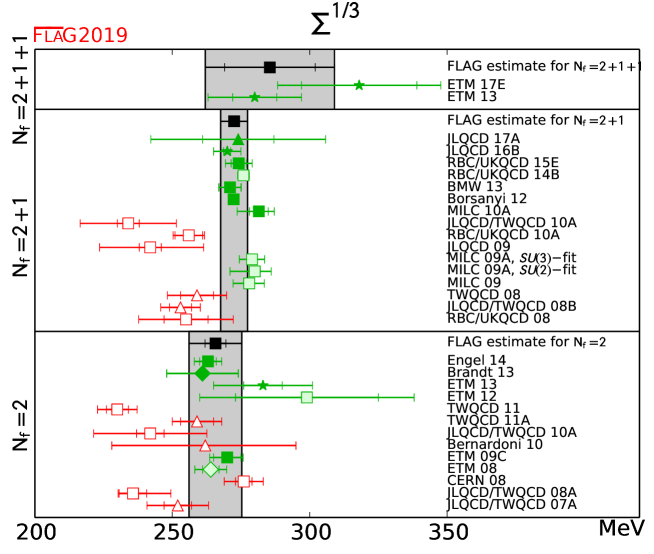
Figure 12: Cubic root of the $SU(2)$ quark condensate $\Sigma\equiv-\langle\bar{u}u\rangle|_{m_{u},m_{d}\to 0}$ in the $\overline{\rm MS}$-scheme, at the renormalization scale $\mu=2\,\mathrm{GeV}$. Green and red squares indicate determinations from correlators in the $p$-regime. Up triangles refer to extractions from the topological susceptibility, diamonds to determinations from the pion form factor, and star symbols refer to the spectral density method.

We begin with a discussion of the lattice results for the $SU(2)$ LEC $\Sigma$. We present the results in Tab. 19 and Fig. 12. We remind the reader that results which include only a statistical error are listed in the table but omitted from the plot. Regarding the $N_{f}=2$ computations there are six entries without a red tag. We form the average based on ETM 09C, ETM 13 (here we deviate from our “superseded” rule, since the two works use different methods), Brandt 13, and Engel 14. Here and in the following we take into account that ETM 09C, ETM 13 share configurations, and the same statement holds true for Brandt 13 and Engel 14. Regarding the $N_{f}=2+1$ computations there are six published or updated papers (MILC 10A, Borsanyi 12, BMW 13, RBC/UKQCD 15E, JLQCD 16B and JLQCD 17A) that qualify for the $N_{f}=2+1$ average. Here we deviate again from the “superseded” rule, since JLQCD 17A [Aoki:2017paw] uses a completely different methodology than JLQCD 16B [Cossu:2016eqs]. Unfortunately, the new error-bar (from an indirect determination, via the topological susceptibility) is about an order of magnitude larger than the old one, hence it barely affects our average. Finally, the single complete $N_{f}=2+1+1$ calculation available so far, ETM 13 [Cichy:2013gja], was recently complemented by ETM 17E [Alexandrou:2017bzk]. Again we deviate from the “supersede” rule, since both authors and methodologies differ.

In slight deviation from the general recipe outlined in Sec. 2.2 we use these values as a basis for our estimates (as opposed to averages) of the $N_{f}=2$, $N_{f}=2+1$, and $N_{f}=2+1+1$ condensates. In each case the central value is obtained from our standard averaging procedure, but the (symmetrical) error is just the median of the overall uncertainties of all contributing results (see the comment below for details). This leads to the values

$$N_{f}=2: \Sigma^{1/3} =266(10)\,\mathrm{MeV} \,\mathrm{Refs.}~{}\mbox{\cite[cite]{[\@@bibref{Number}{Baron:2009wt,Cichy:2013gja,Brandt:2013dua,Engel:2014eea}{}{}]}},$$

$$N_{f}=2+1: \Sigma^{1/3} =272(5)\,\mathrm{MeV} \,\mathrm{Refs.}~{}\mbox{\cite[cite]{[\@@bibref{Number}{Bazavov:2010yq,Borsanyi:2012zv,Durr:2013goa,Boyle:2015exm,Cossu:2016eqs,Aoki:2017paw}{}{}]}},$$ (122)

$$N_{f}=2+1+1: \Sigma^{1/3} =286(23)\,\mathrm{MeV} \,\mathrm{Refs.}~{}\mbox{\cite[cite]{[\@@bibref{Number}{Cichy:2013gja,Alexandrou:2017bzk}{}{}]}},$$

in the ${\overline{\mathrm{MS}}}$ scheme at the renormalization scale $2\,\mathrm{GeV}$, where the errors include both statistical and systematic uncertainties. In accordance with our guidelines we ask the reader to cite the appropriate set of references as indicated in Eq. (5.2.2) when using these numbers.

As a rationale for using estimates (as opposed to averages) for $N_{f}=2$, $N_{f}=2+1$, and $N_{f}=2+1+1$, we add that for $\Sigma^{1/3}|_{N_{f}=2}$, $\Sigma^{1/3}|_{N_{f}=2+1}$, and $\Sigma^{1/3}|_{N_{f}=2+1+1}$ the standard averaging method would yield central values as quoted in Eq. (5.2.2), but with (overall) uncertainties of $4\,\mathrm{MeV}$, $1\,\mathrm{MeV}$, and $16\,\mathrm{MeV}$, respectively. It is not entirely clear to us that the scale is sufficiently well known in all contributing works to warrant a precision of up to 0.37% on our $\Sigma^{1/3}$, and a similar statement can be made about the level of control over the convergence of the chiral expansion. The aforementioned uncertainties would tend to suggest an $N_{f}$-dependence of the $SU(2)$ chiral condensate, which (especially in view of similar issues with other LECs, see below) seems premature to us. Therefore we choose to form the central value of our estimate with the standard averaging procedure, but its uncertainty is taken as the median of the uncertainties of the participating results. We hope that future high-quality determinations (with any of $N_{f}=2$, $N_{f}=2+1$, or $N_{f}=2+1+1$) will help determine whether there is a noticeable $N_{f}$-dependence of the $SU(2)$ chiral condensate or not.

Collaboration	Ref.	$N_{f}$	publication status	chiral extrapolation	continuum extrapolation	finite volume	$F$	$F_{\pi}/F$
ETM 11	[Baron:2011sf]	2+1+1	C	$\circ$	$\bigstar$	$\circ$	85.60(4)(13)	1.077(2)(2)
ETM 10	[Baron:2010bv]	2+1+1	A	$\circ$	$\blacksquare$	$\bigstar$	85.66(6)(13)	1.076(2)(2)
RBC/UKQCD 15E	[Boyle:2015exm]	2+1	A	$\bigstar$	$\bigstar$	$\bigstar$	85.8(1.1)(1.5)	1.0641(21)(49)
RBC/UKQCD 14B	[Blum:2014tka]	2+1	A	$\bigstar$	$\bigstar$	$\bigstar$	86.63(12)(13)	1.0645(15)(0)
BMW 13	[Durr:2013goa]	2+1	A	$\bigstar$	$\bigstar$	$\bigstar$	88.0(1.3)(0.3)	1.055(7)(2)
Borsanyi 12	[Borsanyi:2012zv]	2+1	A	$\circ$	$\circ$	$\bigstar$	86.78(05)(25)	1.0627(06)(27)
NPLQCD 11	[Beane:2011zm]	2+1	A	$\circ$	$\circ$	$\circ$	86.8(2.1)$\binom{+3.3}{-3.4}$	1.062(26)$\binom{+42}{-40}$
MILC 10	[Bazavov:2010hj]	2+1	C	$\circ$	$\bigstar$	$\bigstar$	87.0(4)(5)	1.060(5)(6)
MILC 10A	[Bazavov:2010yq]	2+1	C	$\circ$	$\bigstar$	$\bigstar$	87.5(1.0)$\binom{+0.7}{-2.6}$	1.054(12)$\binom{+31}{-09}$
MILC 09A, $SU(3)$-fit	[Bazavov:2009fk]	2+1	C	$\circ$	$\bigstar$	$\bigstar$	86.8(2)(4)	1.062(1)(3)
MILC 09A, $SU(2)$-fit	[Bazavov:2009fk]	2+1	C	$\circ$	$\bigstar$	$\bigstar$	87.4(0.6)$\binom{+0.9}{-1.0}$	1.054(7)$\binom{+12}{-11}$
MILC 09	[Bazavov:2009bb]	2+1	A	$\circ$	$\bigstar$	$\bigstar$	87.66(17)$\binom{+28}{-52}$	1.052(2)$\binom{+6}{-3}$
PACS-CS 08, $SU(3)$-fit	[Aoki:2008sm]	2+1	A	$\bigstar$	$\blacksquare$	$\blacksquare$	90.3(3.6)	1.062(8)
PACS-CS 08, $SU(2)$-fit	[Aoki:2008sm]	2+1	A	$\bigstar$	$\blacksquare$	$\blacksquare$	89.4(3.3)	1.060(7)
RBC/UKQCD 08	[Allton:2008pn]	2+1	A	$\circ$	$\blacksquare$	$\circ$	81.2(2.9)(5.7)	1.080(8)
ETM 15A	[Abdel-Rehim:2015pwa]	2	A	$\bigstar$	$\blacksquare$	$\circ$	86.3(2.8)	1.069(35)
Engel 14	[Engel:2014eea]	2	A	$\bigstar$	$\bigstar$	$\bigstar$	85.8(0.7)(2.0)	1.075(09)(25)
Brandt 13	[Brandt:2013dua]	2	A	$\circ$	$\bigstar$	$\circ$	84(8)(2)	1.080(16)(6)
QCDSF 13	[Horsley:2013ayv]	2	A	$\bigstar$	$\circ$	$\circ$	86(1)	1.07(1)
TWQCD 11	[Chiu:2011bm]	2	A	$\circ$	$\blacksquare$	$\blacksquare$	83.39(35)(38)	1.106(5)(5)
ETM 09C	[Baron:2009wt]	2	A	$\circ$	$\bigstar$	$\circ$	85.91(07)$\binom{+78}{-07}$	1.0755(6)$\binom{+08}{-94}$
ETM 08	[Frezzotti:2008dr]	2	A	$\circ$	$\circ$	$\circ$	86.6(7)(7)	1.067(9)(9)
Hasenfratz 08	[Hasenfratz:2008ce]	2	A	$\circ$	$\blacksquare$	$\circ$	90(4)	1.02(5)
JLQCD/TWQCD 08A	[Noaki:2008iy]	2	A	$\circ$	$\blacksquare$	$\blacksquare$	79.0(2.5)(0.7)$\binom{+4.2}{-0.0}$	1.167(37)(10)$\binom{+02}{-62}$
JLQCD/TWQCD 07	[Fukaya:2007pn]	2	A	$\circ$	$\blacksquare$	$\blacksquare$	87.3(5.6)	1.06(7)
Colangelo 03	[Colangelo:2003hf]						86.2(5)	1.0719(52)

Table 20: Results for the $SU(2)$ low-energy constant $F$ (in MeV) and for the ratio $F_{\pi}/F$. All ETM values that were available only in $r_{0}$ units were converted on the basis of $r_{0}=0.48(2)\,\mathrm{fm}$ [Aoki:2009sc, Bazavov:2014pvz, Abdel-Rehim:2015pwa], with this error being added in quadrature to any existing systematic error. Numbers in slanted fonts have been calculated by us, based on $\sqrt{2}F_{\pi}^{\mathrm{phys}}=130.41(20)\,\mathrm{MeV}$ [Agashe:2014kda], with this error being added in quadrature to any existing systematic error (otherwise to the statistical error). The systematic error in ETM 11 has been carried over from ETM 10.

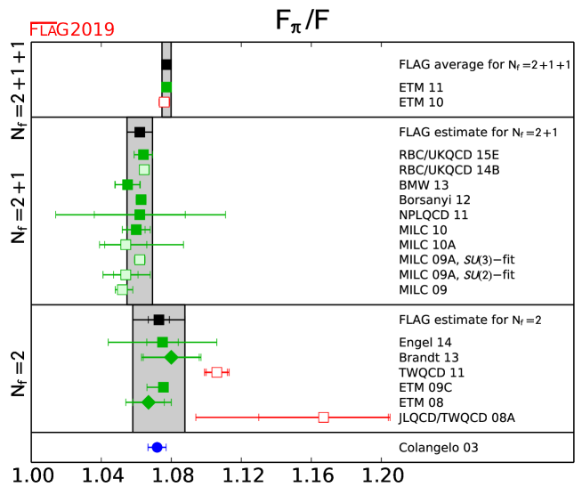
Figure 13: Comparison of the results for the ratio of the physical pion decay constant $F_{\pi}$ and the leading-order $SU(2)$ low-energy constant $F$. The meaning of the symbols is the same as in Fig. 12.

The next quantity considered is $F$, i.e., the pion decay constant in the $SU(2)$ chiral limit ($m_{ud}\to 0$, at fixed physical $m_{s}$ for $N_{f}>2$ simulations). As argued on previous occasions we tend to give preference to $F_{\pi}/F$ (here the numerator is meant to refer to the physical-pion-mass point) wherever it is available, since often some of the systematic uncertainties are mitigated. We collect the results in Tab. 20 and Fig. 13. In those cases where the collaboration provides only $F$, the ratio is computed on the basis of the phenomenological value of $F_{\pi}$, and the respective entries in Tab. 20 are in slanted fonts. We encourage authors to provide both $F$ and $F_{\pi}/F$ from their analysis, since the ratio is less dependent on the scale setting, and errors tend to partially cancel. Among the $N_{f}=2$ determinations five (ETM 08, ETM 09C, QCDSF 13, Brandt 13 and Engel 14) are without red tags. Since the third one is without systematic error, only four of them enter the average. Among the $N_{f}=2+1$ determinations five values (MILC 10 as an update of MILC 09, NPLQCD 11, Borsanyi 12, BMW 13, and RBC/UKQCD 15E) contribute to the average. Here and in the following we take into account that MILC 10 and NPLQCD 11 share configurations. Finally, there is a single $N_{f}=2+1+1$ determination (ETM 11) which forms the current best estimate in this category.

In analogy to the condensates discussed above, we use these values as a basis for our estimates (as opposed to averages) of the decay constant ratios

$$N_{f}=2: {F_{\pi}}/{F} =1.073(15) \,\mathrm{Refs.}~{}\mbox{\cite[cite]{[\@@bibref{Number}{Frezzotti:2008dr,Baron:2009wt,Brandt:2013dua,Engel:2014eea}{}{}]}},$$

$$N_{f}=2+1: {F_{\pi}}/{F} =1.062(7) \,\mathrm{Refs.}~{}\mbox{\cite[cite]{[\@@bibref{Number}{Bazavov:2010hj,Beane:2011zm,Borsanyi:2012zv,Durr:2013goa,Boyle:2015exm}{}{}]}},$$ (123)

$$N_{f}=2+1+1: {F_{\pi}}/{F} =1.077(3) \ref{~}\mbox{\cite[cite]{[\@@bibref{Number}{Baron:2011sf}{}{}]}},$$

where the errors include both statistical and systematic uncertainties. We ask the reader to cite the appropriate set of references as indicated in Eq. (5.2.2) when using these numbers. For $N_{f}=2$ and $N_{f}=2+1$ these estimates are obtained through the well-defined procedure described next to Eq. (5.2.2). For $N_{f}=2+1+1$ the result of ETM 11 (as an update to ETM 10) is the only one available.

For $N_{f}=2$ and $N_{f}=2+1$ the standard averaging method would yield the central values as quoted in Eq. (5.2.2), but with (overall) uncertainties of $6$ and $1$, respectively, on the last digit quoted. In this particular case the single $N_{f}=2+1+1$ determination lies significantly higher than the $N_{f}=2+1$ average (with the small error-bar), basically on par with the $N_{f}=2$ average (ditto), and this makes such a standard average look even more suspicious to us. At the very least, one should wait for one more qualifying $N_{f}=2+1+1$ determination before attempting any conclusions about the $N_{f}$-dependence of $F_{\pi}/F$. While we are not aware of any theorem that excludes a nonmonotonic behavior in $N_{f}$ of a LEC, standard physics reasoning would suggest that quark-loop effects become smaller with increasing quark mass, hence a dynamical charm quark will influence LECs less significantly than a dynamical strange quark, and even the latter one seems to bring rather small shifts. As a result, we feel that a nonmonotonic behavior of $F_{\pi}/F$ with $N_{f}$, once established, would represent a noteworthy finding. We hope this reasoning explains why we prefer to stay in Eq. (5.2.2) with estimates that obviously are on the conservative side.

5.2.3 Results for the NLO $SU(2)$ LECs

Collaboration	Ref.	$N_{f}$	publication status	chiral extrapolation	continuum extrapolation	finite volume	$\bar{\ell}_{3}$	$\bar{\ell}_{4}$
ETM 11	[Baron:2011sf]	2+1+1	C	$\circ$	$\bigstar$	$\circ$	3.53(5)(26)	4.73(2)(10)
ETM 10	[Baron:2010bv]	2+1+1	A	$\circ$	$\blacksquare$	$\bigstar$	3.70(7)(26)	4.67(3)(10)
RBC/UKQCD 15E	[Boyle:2015exm]	2+1	A	$\bigstar$	$\bigstar$	$\bigstar$	2.81(19)(45)	4.02(8)(24)
RBC/UKQCD 14B	[Blum:2014tka]	2+1	A	$\bigstar$	$\bigstar$	$\bigstar$	2.73(13)(0)	4.113(59)(0)
BMW 13	[Durr:2013goa]	2+1	A	$\bigstar$	$\bigstar$	$\bigstar$	2.5(5)(4)	3.8(4)(2)
RBC/UKQCD 12	[Arthur:2012opa]	2+1	A	$\bigstar$	$\circ$	$\bigstar$	2.91(23)(07)	3.99(16)(09)
Borsanyi 12	[Borsanyi:2012zv]	2+1	A	$\circ$	$\circ$	$\bigstar$	3.16(10)(29)	4.03(03)(16)
NPLQCD 11	[Beane:2011zm]	2+1	A	$\circ$	$\circ$	$\circ$	4.04(40)$\binom{+73}{-55}$	4.30(51)$\binom{+84}{-60}$
MILC 10	[Bazavov:2010hj]	2+1	C	$\circ$	$\bigstar$	$\bigstar$	3.18(50)(89)	4.29(21)(82)
MILC 10A	[Bazavov:2010yq]	2+1	C	$\circ$	$\bigstar$	$\bigstar$	2.85(81)$\binom{+37}{-92}$	3.98(32)$\binom{+51}{-28}$
RBC/UKQCD 10A	[Aoki:2010dy]	2+1	A	$\circ$	$\circ$	$\blacksquare$	2.57(18)	3.83(9)
MILC 09A, $SU(3)$-fit	[Bazavov:2009fk]	2+1	C	$\circ$	$\bigstar$	$\bigstar$	3.32(64)(45)	4.03(16)(17)
MILC 09A, $SU(2)$-fit	[Bazavov:2009fk]	2+1	C	$\circ$	$\bigstar$	$\bigstar$	3.0(6)$\binom{+9}{-6}$	3.9(2)(3)
PACS-CS 08, $SU(3)$-fit	[Aoki:2008sm]	2+1	A	$\bigstar$	$\blacksquare$	$\blacksquare$	3.47(11)	4.21(11)
PACS-CS 08, $SU(2)$-fit	[Aoki:2008sm]	2+1	A	$\bigstar$	$\blacksquare$	$\blacksquare$	3.14(23)	4.04(19)
RBC/UKQCD 08	[Allton:2008pn]	2+1	A	$\circ$	$\blacksquare$	$\circ$	3.13(33)(24)	4.43(14)(77)
ETM 15A	[Abdel-Rehim:2015pwa]	2	A	$\bigstar$	$\blacksquare$	$\circ$		3.3(4)
Gülpers 15	[Gulpers:2015bba]	2	A	$\bigstar$	$\bigstar$	$\bigstar$		4.54(30)(0)
Gülpers 13	[Gulpers:2013uca]	2	A	$\circ$	$\blacksquare$	$\circ$		4.76(13)
Brandt 13	[Brandt:2013dua]	2	A	$\circ$	$\bigstar$	$\circ$	3.0(7)(5)	4.7(4)(1)
QCDSF 13	[Horsley:2013ayv]	2	A	$\bigstar$	$\circ$	$\circ$		4.2(1)
Bernardoni 11	[Bernardoni:2011kd]	2	C	$\circ$	$\blacksquare$	$\blacksquare$	4.46(30)(14)	4.56(10)(4)
TWQCD 11	[Chiu:2011bm]	2	A	$\circ$	$\blacksquare$	$\blacksquare$	4.149(35)(14)	4.582(17)(20)
ETM 09C	[Baron:2009wt]	2	A	$\circ$	$\bigstar$	$\circ$	3.50(9)$\binom{+09}{-30}$	4.66(4)$\binom{+04}{-33}$
JLQCD/TWQCD 09	[JLQCD:2009qn]	2	A	$\circ$	$\blacksquare$	$\blacksquare$		4.09(50)(52)
ETM 08	[Frezzotti:2008dr]	2	A	$\circ$	$\circ$	$\circ$	3.2(8)(2)	4.4(2)(1)
JLQCD/TWQCD 08A	[Noaki:2008iy]	2	A	$\circ$	$\blacksquare$	$\blacksquare$	3.38(40)(24)$\binom{+31}{-00}$	4.12(35)(30)$\binom{+31}{-00}$
CERN-TOV 06	[DelDebbio:2006cn]	2	A	$\circ$	$\blacksquare$	$\blacksquare$	3.0(5)(1)
Colangelo 01	[Colangelo:2001df]							4.4(2)
Gasser 84	[Gasser:1983yg]						2.9(2.4)	4.3(9)

Table 21: Results for the $SU(2)$ NLO low-energy constants $\bar{\ell}_{3}$ and $\bar{\ell}_{4}$. For comparison, the last two lines show results from phenomenological analyses. The systematic error in ETM 11 has been carried over from ETM 10.

Figure 14: Effective coupling constants $\bar{\ell}_{3}$, $\bar{\ell}_{4}$ and $\bar{\ell}_{6}$. Squares indicate determinations from correlators in the $p$-regime, diamonds refer to determinations from the pion form factor.

We move on to a discussion of the lattice results for the NLO LECs $\bar{\ell}_{3}$ and $\bar{\ell}_{4}$. We remind the reader that on the lattice the former LEC is obtained as a result of the tiny deviation from linearity seen in $M_{\pi}^{2}$ versus $Bm_{ud}$, whereas the latter LEC is extracted from the curvature in $F_{\pi}$ versus $Bm_{ud}$. The available determinations are presented in Tab. 21 and Fig. 1. Among the $N_{f}=2$ determinations ETM 08, ETM 09C, Brandt 13, and Gülpers 15 come with a systematic uncertainty and without red tags. Given that the former two use different approaches, all four determinations enter our average. The colour coding of the $N_{f}=2+1$ results looks very promising; there is a significant number of lattice determinations without any red tag. Applying our superseding rule, MILC 10 (as an update to MILC 09), NPLQCD 11, Borsanyi 12, BMW 13, and RBC/UKQCD 15E contribute to the average. For $N_{f}=2+1+1$ there is only the single work ETM 11 (as an update to ETM 10).

In analogy to our processing of the LECs at LO, we use these determinations as the basis of our estimate (as opposed to average) of the NLO quantities

$$N_{f}=2: \bar{\ell}_{3} =3.41(82) \,\mathrm{Refs.}~{}\mbox{\cite[cite]{[\@@bibref{Number}{Frezzotti:2008dr,Baron:2009wt,Brandt:2013dua}{}{}]}},$$

$$N_{f}=2+1: \bar{\ell}_{3} =3.07(64) \,\mathrm{Refs.}~{}\mbox{\cite[cite]{[\@@bibref{Number}{Bazavov:2010hj,Beane:2011zm,Borsanyi:2012zv,Durr:2013goa,Boyle:2015exm}{}{}]}},$$ (124)

$$N_{f}=2+1+1: \bar{\ell}_{3} =3.53(26)$$ LABEL:~[Baron:2011sf]

$$N_{f}=2: \bar{\ell}_{4} =4.40(28) \,\mathrm{Refs.}~{}\mbox{\cite[cite]{[\@@bibref{Number}{Frezzotti:2008dr,Baron:2009wt,Brandt:2013dua,Gulpers:2015bba}{}{}]}},$$

$$N_{f}=2+1: \bar{\ell}_{4} =4.02(45) \,\mathrm{Refs.}~{}\mbox{\cite[cite]{[\@@bibref{Number}{Bazavov:2010hj,Beane:2011zm,Borsanyi:2012zv,Durr:2013goa,Boyle:2015exm}{}{}]}},$$ (125)

$$N_{f}=2+1+1: \bar{\ell}_{4} =4.73(10)$$ LABEL:~[Baron:2011sf]

where the errors include both statistical and systematic uncertainties. Again we ask the reader to cite the appropriate set of references as indicated in Eq. (1) or Eq. (1) when using these numbers. For $N_{f}=2$ and $N_{f}=2+1$ these estimates are obtained through the well-defined procedure described next to Eq. (5.2.2). For $N_{f}=2+1+1$ once again ETM 11 (as an update to ETM 10) is the single reference available.

We remark that our preprocessing procedure symmetrizes the asymmetric error of ETM 09C with a slight adjustment of the central value. Regarding the difference between the estimates as given in Eqs. (1, 1) and the result of the standard averaging procedure we add that the latter would yield the overall uncertainties $25$ and $12$ for $\bar{\ell}_{3}$, and the overall uncertainties $17$ and $5$ for $\bar{\ell}_{4}$. In all cases the central value would be unchanged. Especially for $\bar{\ell}_{4}$ such numbers would suggest a clear difference between the value with $N_{f}=2$ dynamical flavours and the one at $N_{f}=2+1$. Similarly to what happened with $F_{\pi}/F$, the single determination with $N_{f}=2+1+1$ is more on the $N_{f}=2$ side, which, if confirmed, would suggest a nonmonotonicity of a $\chi$PT LEC with $N_{f}$. Again we think that currently such a conclusion would be premature, and this is why we give preference to the estimates quoted in Eqs. (1, 1).

From a more phenomenological point of view there is a notable difference between $\bar{\ell}_{3}$ and $\bar{\ell}_{4}$ in Fig. 1. For $\bar{\ell}_{4}$ the precision of the phenomenological determination achieved in Colangelo 01 [Colangelo:2001df] represents a significant improvement compared to Gasser 84 [Gasser:1983yg]. Picking any $N_{f}$, the lattice estimate of $\bar{\ell}_{4}$ is consistent with both of the phenomenological values and comes with an error-bar that is roughly comparable to or somewhat larger than the one in Colangelo 01 [Colangelo:2001df]. By contrast, for $\bar{\ell}_{3}$ the error of an individual lattice computation is usually much smaller than the error of the estimate given in Gasser 84 [Gasser:1983yg], and even our conservative estimates (1) have uncertainties that represent a significant improvement on the error-bar of Gasser 84 [Gasser:1983yg]. Evidently, our hope is that future determinations of $\bar{\ell}_{3},\bar{\ell}_{4}$, with $N_{f}=2$, $N_{f}=2+1$ and $N_{f}=2+1+1$, will allow us to further shrink our error-bars in a future edition of FLAG.

Collaboration	Ref.	$N_{f}$	publication status	chiral extrapolation	continuum extrapolation	finite volume	$\langle r^{2}\rangle_{V}^{\pi}$	$c_{V}$	$\bar{\ell}_{6}$
HPQCD 15B	[Koponen:2015tkr]	2+1+1	A	$\bigstar$	$\circ$	$\bigstar$	0.403(18)(6)
JLQCD 15A, $SU(2)$-fit	[Aoki:2015pba]	2+1	A	$\circ$	$\blacksquare$	$\circ$	0.395(26)(32)		13.49(89)(82)
JLQCD 14	[Fukaya:2014jka]	2+1	A	$\bigstar$	$\blacksquare$	$\blacksquare$	0.49(4)(4)		7.5(1.3)(1.5)
PACS-CS 11A	[Nguyen:2011ek]	2+1	A	$\circ$	$\blacksquare$	$\circ$	0.441(46)
RBC/UKQCD 08A	[Boyle:2008yd]	2+1	A	$\blacksquare$	$\blacksquare$	$\circ$	0.418(31)		12.2(9)
LHP 04	[Bonnet:2004fr]	2+1	A	$\blacksquare$	$\blacksquare$	$\blacksquare$	0.310(46)
ETM 17F	[Alexandrou:2017blh]	2	A	$\bigstar$	$\blacksquare$	$\bigstar$	0.443(21)(20)		16.21(76)(70)
Brandt 13	[Brandt:2013dua]	2	A	$\circ$	$\bigstar$	$\circ$	0.481(33)(13)		15.5(1.7)(1.3)
JLQCD/TWQCD 09	[JLQCD:2009qn]	2	A	$\circ$	$\blacksquare$	$\blacksquare$	0.409(23)(37)	3.22(17)(36)	11.9(0.7)(1.0)
ETM 08	[Frezzotti:2008dr]	2	A	$\circ$	$\circ$	$\circ$	0.456(30)(24)	3.37(31)(27)	14.9(1.2)(0.7)
QCDSF/UKQCD 06A	[Brommel:2006ww]	2	A	$\circ$	$\bigstar$	$\blacksquare$	0.441(19)(63)
Bijnens 98	[Bijnens:1998fm]						0.437(16)	3.85(60)	16.0(0.5)(0.7)
NA7 86	[Amendolia:1986wj]						0.439(8)
Gasser 84	[Gasser:1983yg]								16.5(1.1)

Collaboration	Ref.	$N_{f}$	publication status	chiral extrapolation	continuum extrapolation	finite volume	$\langle r^{2}\rangle_{S}^{\pi}$	$\bar{\ell}_{1}-\bar{\ell}_{2}$
HPQCD 15B	[Koponen:2015tkr]	2+1+1	A	$\bigstar$	$\circ$	$\bigstar$	0.481(37)(50)
RBC/UKQCD 15E	[Boyle:2015exm]	2+1	A	$\bigstar$	$\bigstar$	$\bigstar$		-9.2(4.9)(6.5)
Gülpers 15	[Gulpers:2015bba]	2	A	$\bigstar$	$\bigstar$	$\bigstar$	0.600(52)(0)
Gülpers 13	[Gulpers:2013uca]	2	A	$\circ$	$\blacksquare$	$\circ$	0.637(23)
JLQCD/TWQCD 09	[JLQCD:2009qn]	2	A	$\circ$	$\blacksquare$	$\blacksquare$	0.617(79)(66)	-2.9(0.9)(1.3)
Colangelo 01	[Colangelo:2001df]						0.61(4)	-4.7(6)

Table 22: Top (vector form factor of the pion): Lattice results for the charge radius $\langle r^{2}\rangle_{V}^{\pi}$ (in $\mathrm{fm}^{2}$), the curvature $c_{V}$ (in $\mathrm{GeV}^{-4}$) and the effective coupling constant $\bar{\ell}_{6}$ are compared with the experimental value, as obtained by NA7, and some phenomenological estimates. Bottom (scalar form factor of the pion): Lattice results for the scalar radius $\langle r^{2}\rangle_{S}^{\pi}$ (in $\mathrm{fm}^{2}$) and the combination $\bar{\ell}_{1}-\bar{\ell}_{2}$ are compared with a dispersive calculation of these quantities.

Let us add that Ref. [Doring:2016bdr] determines $\ell_{1},\ell_{2},\ell_{3},\ell_{4}$ (or equivalently $\bar{\ell}_{1},\bar{\ell}_{2},\bar{\ell}_{3},\bar{\ell}_{4}$) individually, with some assumptions and various fits from lattice data at a single lattice spacing and two (heavier than physical) pion masses.

We continue with a discussion of the lattice results for $\bar{\ell}_{6}$ and $\bar{\ell}_{1}-\bar{\ell}_{2}$. The LEC $\bar{\ell}_{6}$ determines the leading contribution in the chiral expansion of the pion vector charge radius, see Eq. (101). Hence from a lattice study of the vector form factor of the pion with several $M_{\pi}$ one may extract the radius $\langle r^{2}\rangle_{V}^{\pi}$, the curvature $c_{V}$ (both at the physical pion-mass point) and the LEC $\bar{\ell}_{6}$ in one go. Similarly, the leading contribution in the chiral expansion of the scalar radius of the pion determines $\bar{\ell}_{4}$, see Eq. (101). This LEC is also present in the pion-mass dependence of $F_{\pi}$, as we have seen. The difference $\bar{\ell}_{1}-\bar{\ell}_{2}$, finally, may be obtained from the momentum dependence of the vector and scalar pion form factors, based on the 2-loop formulae of Ref. [Bijnens:1998fm]. The top part of Tab. 1 collects the results obtained from the vector form factor of the pion (charge radius, curvature and $\bar{\ell}_{6}$). Regarding this low-energy constant two $N_{f}=2$ calculations are published works without a red tag; we thus arrive at the average (actually the first one in the LEC section)

$$N_{f}=2:\hskip 28.45274pt\bar{\ell}_{6}=15.1(1.2)\qquad\,\mathrm{Refs.}~{}\mbox{\cite[cite]{[\@@bibref{Number}{Frezzotti:2008dr,Brandt:2013dua}{}{}]}},$$ (126)

which is represented as a grey band in the last panel of Fig. 1. Here we ask the reader to cite Refs. [Frezzotti:2008dr, Brandt:2013dua] when using this number.

Figure 15: Summary of the pion form factors $\langle r^{2}\rangle_{V}^{\pi}$ (top) and $\langle r^{2}\rangle_{S}^{\pi}$ (bottom).

The experimental information concerning the charge radius is excellent and the curvature is also known very accurately, based on $e^{+}e^{-}$ data and dispersion theory. The vector form factor calculations thus present an excellent testing ground for the lattice methodology. The first data column of Tab. 1 shows that most of the available lattice results pass the test. There is, however, one worrisome point. For $\bar{\ell}_{6}$ the agreement seems less convincing than for the charge radius, even though the two quantities are closely related. In particular the $\bar{\ell}_{6}$ value of JLQCD 14 [Fukaya:2014jka] seems inconsistent with the phenomenological determinations of Refs. [Gasser:1983yg, Bijnens:1998fm], even though its value for $\langle r^{2}\rangle_{V}^{\pi}$ is consistent. So far we have no explanation (other than observing that lattice computations which disagree with the phenomenological determination of $\bar{\ell}_{6}$ tend to have red tags), but we urge the groups to pay special attention to this point. Similarly, the bottom part of Tab. 1 collects the results obtained for the scalar form factor of the pion and the combination $\bar{\ell}_{1}-\bar{\ell}_{2}$ that is extracted from it. A new feature is that Ref. [Koponen:2015tkr] gives both the (flavour) octet and singlet part in $SU(3)$, finding $\langle r^{2}\rangle_{S,\mathrm{octet}}^{\pi}=0.431(38)(46)$ and $\langle r^{2}\rangle_{S,\mathrm{singlet}}^{\pi}=0.506(38)(53)$. For reasons of backward compatibility they also give $\langle r^{2}\rangle_{S,ud}^{\pi}$ defined with a $\bar{u}u+\bar{d}d$ density, and this number is shown in Tab. 1. Another notable feature is that they find the ordering $\langle r^{2}\rangle_{S,\mathrm{conn}}^{\pi}<\langle r^{2}\rangle_{S,\mathrm{octet}}^{\pi}<\langle r^{2}\rangle_{S,ud}^{\pi}<\langle r^{2}\rangle_{S,\mathrm{singlet}}^{\pi}$ [Koponen:2015tkr].

Those data of Tab. 1 that come with a systematic error are shown in Fig. 1. The overall impression is that the majority of lattice results come with a fair assessment of the respective systematic uncertainties. Yet it is clear that it is a nontrivial endeavor to match the precision obtained in experiment and subsequent phenomenological analysis.

Collaboration	Ref.	$N_{f}$	publication status	chiral extrapolation	continuum extrapolation	finite volume	$a_{0}^{0}M_{\pi}$	$\ell_{\pi\pi}^{0}$
Fu 17	[Fu:2017apw]	2+1	A	$\blacksquare$	$\circ$	$\bigstar$	$0.217(9)(5)$	$45.6(7.6)(3.8)$
Fu 13	[Fu:2013ffa]	2+1	A	$\blacksquare$	$\blacksquare$	$\bigstar$	$0.214(4)(7)$	$43.2(3.5)(5.6)$
Fu 11	[Fu:2011bz]	2+1	A	$\blacksquare$	$\blacksquare$	$\bigstar$	$0.186(2)$	$18.7(1.2)$
ETM 16C	[Liu:2016cba]	2	A	$\bigstar$	$\blacksquare$	$\bigstar$	$0.198(9)(6)$	$30(8)(6)$
Colangelo 01	[Colangelo:2001df]						$0.220(5)_{\mathrm{tot}}$
Caprini 11	[Caprini:2011ky]						$0.2198(46)_{\mathrm{stat}}(16)_{\mathrm{syst}}(64)_{\mathrm{th}}$

Collaboration	Ref.	$N_{f}$	publication status	chiral extrapolation	continuum extrapolation	finite volume	$a_{0}^{2}M_{\pi}$	$\ell_{\pi\pi}^{2}$
ETM 15E	[Helmes:2015gla]	2+1+1	A	$\circ$	$\bigstar$	$\bigstar$	$-0.0442(2)(^{4}_{0})$	$3.79(0.61)({}^{+1.34}_{-0.11})$
PACS-CS 13	[Sasaki:2013vxa]	2+1	A	$\bigstar$	$\blacksquare$	$\blacksquare$	$-0.04263(22)(41)$
Fu 13	[Fu:2013ffa]	2+1	A	$\blacksquare$	$\blacksquare$	$\bigstar$	$-0.04430(25)(40)$	$3.27(0.77)(1.12)$
Fu 11	[Fu:2011bz]	2+1	A	$\blacksquare$	$\blacksquare$	$\bigstar$	$-0.0416(2)$	$11.6(9)$
NPLQCD 11A	[Beane:2011sc]	2+1	A	$\blacksquare$	$\blacksquare$	$\bigstar$	$-0.0417(07)(02)(16)$
NPLQCD 07	[Beane:2007xs]	2+1	A	$\blacksquare$	$\blacksquare$	$\blacksquare$	$-0.04330(42)_{\mathrm{tot}}$
NPLQCD 05	[Beane:2005rj]	2+1	A	$\blacksquare$	$\blacksquare$	$\blacksquare$	$-0.0426(06)(03)(18)$
Yagi 11	[Yagi:2011jn]	2	P	$\circ$	$\blacksquare$	$\blacksquare$	$-0.04410(69)(18)$
ETM 09G	[Feng:2009ij]	2	A	$\circ$	$\circ$	$\circ$	$-0.04385(28)(38)$	$4.65(0.85)(1.07)$
CP-PACS 04	[Yamazaki:2004qb]	2	A	$\blacksquare$	$\blacksquare$	$\bigstar$	$-0.0413(29)$
Colangelo 01	[Colangelo:2001df]						$-0.0444(10)_{\mathrm{tot}}$
Caprini 11	[Caprini:2011ky]						$-0.0445(11)_{\mathrm{stat}}(4)_{\mathrm{syst}}(8)_{\mathrm{th}}$

Table 23: Summary of $\pi$-$\pi$ scattering data in the $I=0$ (top) and $I=2$ (bottom) channels. In our view the paper Fu 17 contains one pion mass at $a\simeq 0.09\mathrm{fm}$ and another one at $a\simeq 0.06\mathrm{fm}$. The results of ETM 15E and NPLQCD 11A have been adapted to our sign convention. The results of Refs. [Colangelo:2001df, Caprini:2011ky] allow for a cross-check with phenomenology.

The last set of observables we wish to discuss includes the $\pi$-$\pi$ scattering lengths $a_{0}^{0}$ and $a_{0}^{2}$ in the isopin channels $I=0$ and $I=2$, respectively. As can be seen from Eqs. (108, 110), the $I=0$ scattering length carries information about $\frac{20}{21}\bar{\ell}_{1}+\frac{40}{21}\bar{\ell}_{2}-\frac{5}{14}\bar{\ell}_{3}+2\bar{\ell}_{4}$. And from Eqs. (109, 111) it follows that the $I=2$ counterpart carries information about the linear combination $\frac{4}{3}\bar{\ell}_{1}+\frac{8}{3}\bar{\ell}_{2}-\frac{1}{2}\bar{\ell}_{3}-2\bar{\ell}_{4}$. We prefer quoting the dimensionless products $a_{0}^{I}M_{\pi}$ (at the physical mass point) over the aforementioned linear combinations to ease comparison with phenomenology. In Tab. 1 we summarize the lattice information on $a_{0}^{I=0}M_{\pi}$ and $a_{0}^{I=2}M_{\pi}$ at the physical mass point. We are aware of at least one additional work, Ref. [Bulava:2016mks], which has a technical focus and determines a scattering length away from the physical point, and which, for this reason, is not included in Tab. 1. We remind the reader that a lattice computation of $a_{0}^{I=0}M_{\pi}$ involves quark-loop disconnected contributions, which tend to be very noisy and hence require lots of statistics. To date there are three pioneering calculations, but none of them is free of red tags. The situation is slightly better for $a_{0}^{I=2}M_{\pi}$; there is one computation at $N_{f}=2$ and one at $N_{f}=2+1+1$ that would qualify for a FLAG average. Still, since in the much better populated category of $N_{f}=2+1$ studies there is currently no computation without a red tag, we feel it is appropriate to postpone any form of averaging to the next edition of FLAG, when hopefully qualifying computations (at least for $a_{0}^{I=2}M_{\pi}$) are available at each $N_{f}$ considered.

Figure 16: Summary of the $\pi$-$\pi$ scattering lengths $a_{0}^{0}M_{\pi}$ (top) and $a_{0}^{2}M_{\pi}$ (bottom).

5.2.4 Epilogue

In this subsection there are several quantities for which only one qualifying (“all-green”) determination is available for a given $SU(2)$ LEC. Obviously the phenomenologically oriented reader is encouraged to use such a value (as provided in our tables) and to cite the original work. We hope that the lattice community will come up with further computations, in particular for $N_{f}=2+1+1$, such that a fair comparison of different works is possible at any $N_{f}$, and eventually a statement can be made about the presence or absence of an $N_{f}$-dependence of $SU(2)$ LECs.

What can be learned about the convergence pattern of $SU(2)$ $\chi$PT from varying the fit ranges (in $m_{ud}$) of the pion mass and decay constant (i.e., the quantities from which $\bar{\ell}_{3},\bar{\ell}_{4}$ are derived) is discussed in Ref. [Durr:2014oba], where also the usefulness of comparing results from the $x$ and the $\xi$ expansion (with material taken from Ref. [Durr:2013goa]) is emphasized.

Perhaps the most important physics result of this subsection is that the lattice simulations confirm the approximate validity of the Gell-Mann-Oakes-Renner formula and show that the square of the pion mass indeed grows in proportion to $m_{ud}$. The formula represents the leading term of the chiral series and necessarily receives corrections from higher orders. At first nonleading order, the correction is determined by the effective coupling constant $\bar{\ell}_{3}$. The results collected in Tab. 21 and in the top panel of Fig. 1 show that $\bar{\ell}_{3}$ is now known quite well. They corroborate the conclusion drawn already in Ref. [Durr:2002zx]: the lattice confirms the estimate of $\bar{\ell}_{3}$ derived in Ref. [Gasser:1983yg]. In the graph of $M_{\pi}^{2}$ versus $m_{ud}$, the values found on the lattice for $\bar{\ell}_{3}$ correspond to remarkably little curvature. In other words, the Gell-Mann-Oakes-Renner formula represents a reasonable first approximation out to values of $m_{ud}$ that exceed the physical value by an order of magnitude.

As emphasized by Stern and collaborators [Fuchs:1991cq, Stern:1993rg, DescotesGenon:1999uh], the analysis in the framework of $\chi$PT is coherent only if ($i$) the leading term in the chiral expansion of $M_{\pi}^{2}$ dominates over the remainder and ($ii$) the ratio $m_{s}/m_{ud}$ is close to the value $25.6$ that follows from Weinberg’s leading-order formulae. In order to investigate the possibility that one or both of these conditions might fail, the authors proposed a more general framework, referred to as “generalized $\chi$PT”, which includes (standard) $\chi$PT as a special case. The results found on the lattice demonstrate that QCD does satisfy both of the above conditions. Hence, in the context of QCD, the proposed generalization of the effective theory does not appear to be needed. There is a modified version, however, referred to as “re-summed $\chi$PT” [Bernard:2010ex], which is motivated by the possibility that the Zweig-rule violating couplings $L_{4}$ and $L_{6}$ might be larger than expected. The available lattice data does not support this possibility, but they do not rule it out either (see Sec. 5.3 for details).

5.3 Extraction of $SU(3)$ low-energy constants

To date, there are three comprehensive $SU(3)$ papers with results based on lattice QCD with $N_{f}\!=\!2+1$ dynamical flavours [Allton:2008pn, Aoki:2008sm, Bazavov:2009bb], and one more with results based on $N_{f}\!=\!2+1+1$ dynamical flavours [Dowdall:2013rya]. It is an open issue whether the data collected at $m_{s}\simeq m_{s}^{\mathrm{phys}}$ allows for an unambiguous determination of $SU(3)$ low-energy constants (cf. the discussion in Ref. [Allton:2008pn]). To make definite statements one needs data at considerably smaller $m_{s}$, and so far only MILC has some [Bazavov:2009bb]. We are aware of a few papers with a result on one $SU(3)$ low-energy constant each, which we list for completeness. Some particulars of the computations are listed in Tab. 24.

5.3.1 Results for the LO and NLO $SU(3)$ LECs

Collaboration	Ref.	$N_{f}$	publication status	chiral extrapolation	continuum extrapolation	finite volume	$F_{0}$	$F/F_{0}$	$B/B_{0}$
JLQCD/TWQCD 10A	[Fukaya:2010na]	3	A	$\blacksquare$	$\blacksquare$	$\blacksquare$	71(3)(8)
MILC 10	[Bazavov:2010hj]	2+1	C	$\circ$	$\bigstar$	$\bigstar$	80.3(2.5)(5.4)
MILC 09A	[Bazavov:2009fk]	2+1	C	$\circ$	$\bigstar$	$\bigstar$	78.3(1.4)(2.9)	1.104(3)(41)	1.21(4)$\binom{+5}{-6}$
MILC 09	[Bazavov:2009bb]	2+1	A	$\circ$	$\bigstar$	$\bigstar$		1.15(5)$\binom{+13}{-03}$	1.15(16)$\binom{+39}{-13}$
PACS-CS 08	[Aoki:2008sm]	2+1	A	$\bigstar$	$\blacksquare$	$\blacksquare$	83.8(6.4)	1.078(44)	1.089(15)
RBC/UKQCD 08	[Allton:2008pn]	2+1	A	$\circ$	$\blacksquare$	$\circ$	66.1(5.2)	1.229(59)	1.03(05)

Collaboration	Ref.	$N_{f}$	publication status	chiral extrapolation	continuum extrapolation	finite volume	renormalization	$\Sigma_{0}^{1/3}$	$\Sigma/\Sigma_{0}$
JLQCD/TWQCD 10A	[Fukaya:2010na]	3	A	$\blacksquare$	$\blacksquare$	$\blacksquare$	$\bigstar$	214(6)(24)	1.31(13)(52)
MILC 09A	[Bazavov:2009fk]	2+1	C	$\circ$	$\bigstar$	$\bigstar$	$\circ$	245(5)(4)(4)	1.48(9)(8)(10)
MILC 09	[Bazavov:2009bb]	2+1	A	$\circ$	$\bigstar$	$\bigstar$	$\circ$	242(9)$\binom{+05}{-17}$(4)	1.52(17)$\binom{+38}{-15}$
PACS-CS 08	[Aoki:2008sm]	2+1	A	$\bigstar$	$\blacksquare$	$\blacksquare$	$\blacksquare$	290(15)	1.245(10)
RBC/UKQCD 08	[Allton:2008pn]	2+1	A	$\circ$	$\blacksquare$	$\circ$	$\bigstar$		1.55(21)

Table 24: Lattice results for the low-energy constants $F_{0}$, $B_{0}$ (in MeV) and $\Sigma_{0}\!\equiv\!F_{0}^{2}B_{0}$, which specify the effective $SU(3)$ Lagrangian at leading order. The ratios $F/F_{0}$, $B/B_{0}$, $\Sigma/\Sigma_{0}$, which compare these with their $SU(2)$ counterparts, indicate the strength of the Zweig-rule violations in these quantities (in the large-$N_{c}$ limit, they tend to unity). Numbers in slanted fonts are calculated by us, from the information given in the references.

Collaboration	Ref.	$N_{f}$	publication status	chiral extrapolation	continuum extrapolation	finite volume	$10^{3}L_{4}$	$\rule{2.84544pt}{0.0pt}10^{3}L_{6}$	$10^{3}(2L_{6}\!-\!L_{4})$
HPQCD 13A	[Dowdall:2013rya]	2+1+1	A	$\bigstar$	$\circ$	$\bigstar$	0.09(34)	0.16(20)	0.22(17)
JLQCD/TWQCD 10A	[Fukaya:2010na]	3	A	$\blacksquare$	$\blacksquare$	$\blacksquare$		0.03(7)(17)
MILC 10	[Bazavov:2010hj]	2+1	C	$\circ$	$\bigstar$	$\bigstar$	-0.08(22)$\binom{+57}{-33}$	-0.02(16)$\binom{+33}{-21}$	0.03(24)$\binom{+32}{-27}$
MILC 09A	[Bazavov:2009fk]	2+1	C	$\circ$	$\bigstar$	$\bigstar$	0.04(13)(4)	0.07(10)(3)	0.10(12)(2)
MILC 09	[Bazavov:2009bb]	2+1	A	$\circ$	$\bigstar$	$\bigstar$	0.1(3)$\binom{+3}{-1}$	0.2(2)$\binom{+2}{-1}$	0.3(1)$\binom{+2}{-3}$
PACS-CS 08	[Aoki:2008sm]	2+1	A	$\bigstar$	$\blacksquare$	$\blacksquare$	-0.06(10)(–)	0.02(5)(–)	0.10(2)(–)
RBC/UKQCD 08	[Allton:2008pn]	2+1	A	$\circ$	$\blacksquare$	$\circ$	0.14(8)(–)	0.07(6)(–)	0.00(4)(–)
Bijnens 11	[Bijnens:2011tb]						0.75(75)	0.29(85)	-0.17(1.86)
Gasser 85	[Gasser:1984gg]						-0.3(5)	-0.2(3)	-0.1(8)
Collaboration	Ref.	$N_{f}$					$10^{3}L_{5}$	$10^{3}L_{8}$	$10^{3}(2L_{8}\!-\!L_{5})$
HPQCD 13A	[Dowdall:2013rya]	2+1+1	A	$\bigstar$	$\circ$	$\bigstar$	1.19(25)	0.55(15)	-0.10(20)
MILC 10	[Bazavov:2010hj]	2+1	C	$\circ$	$\bigstar$	$\bigstar$	0.98(16)$\binom{+28}{-41}$	0.42(10)$\binom{+27}{-23}$	-0.15(11)$\binom{+45}{-19}$
MILC 09A	[Bazavov:2009fk]	2+1	C	$\circ$	$\bigstar$	$\bigstar$	0.84(12)(36)	0.36(5)(7)	-0.12(8)(21)
MILC 09	[Bazavov:2009bb]	2+1	A	$\circ$	$\bigstar$	$\bigstar$	1.4(2)$\binom{+2}{-1}$	0.8(1)(1)	0.3(1)(1)
PACS-CS 08	[Aoki:2008sm]	2+1	A	$\bigstar$	$\blacksquare$	$\blacksquare$	1.45(7)(–)	0.62(4)(–)	-0.21(3)(–)
RBC/UKQCD 08	[Allton:2008pn]	2+1	A	$\circ$	$\blacksquare$	$\circ$	0.87(10)(–)	0.56(4)(–)	0.24(4)(–)
NPLQCD 06	[Beane:2006kx]	2+1	A	$\blacksquare$	$\blacksquare$	$\blacksquare$	1.42(2)$\binom{+18}{-54}$
Bijnens 11	[Bijnens:2011tb]						0.58(13)	0.18(18)	-0.22(38)
Gasser 85	[Gasser:1984gg]						1.4(5)	0.9(3)	0.4(8)

Table 25: Low-energy constants of the $SU(3)$ Lagrangian at NLO with running scale $\mu\!=\!770\,\mathrm{MeV}$ (the values in Refs. [Dowdall:2013rya, Bazavov:2010hj, Bazavov:2009bb, Bazavov:2009fk, Gasser:1984gg] are evolved accordingly). The MILC 10 entry for $L_{6}$ is obtained from their results for $2L_{6}\!-\!L_{4}$ and $L_{4}$ (similarly for other entries in slanted fonts).

Collaboration	Ref.	$N_{f}$	publication status	chiral extrapolation	continuum extrapolation	finite volume	$10^{3}L_{9}$	$\rule{2.84544pt}{0.0pt}10^{3}L_{10}$
Boito 15	[Boito:2015fra]	2+1	A	$\bigstar$	$\blacksquare$	$\bigstar$		-3.50(17)
JLQCD 15A	[Aoki:2015pba]	2+1	A	$\circ$	$\blacksquare$	$\circ$	4.6(1.1)$\binom{+0.1}{-0.5}$(0.4)
Boyle 14	[Boyle:2014pja]	2+1	A	$\bigstar$	$\circ$	$\bigstar$		-3.46(32)
JLQCD 14	[Fukaya:2014jka]	2+1	A	$\bigstar$	$\blacksquare$	$\blacksquare$	2.4(0.8)(1.0)
RBC/UKQCD 09	[Boyle:2009xi]	2+1	A	$\circ$	$\blacksquare$	$\circ$		-5.7(11)(07)
RBC/UKQCD 08A	[Boyle:2008yd]	2+1	A	$\blacksquare$	$\blacksquare$	$\circ$	3.08(23)(51)
JLQCD 08A	[Shintani:2008qe]	2	A	$\circ$	$\blacksquare$	$\blacksquare$		-5.2(2)$\binom{+5}{-3}$
Bijnens 02	[Bijnens:2002hp]						5.93(43)
Davier 98	[Davier:1998dz]							-5.13(19)
Gasser 85	[Gasser:1984gg]						6.9(7)	-5.5(7)

Table 26: Low-energy constants of the $SU(3)$ Lagrangian at NLO with running scale $\mu\!=\!770\,\mathrm{MeV}$ (the values in Ref. [Gasser:1984gg] are evolved accordingly). The JLQCD 08A result for $\ell_{5}(770\,\mathrm{MeV})$ [despite the paper saying $L_{10}(770\,\mathrm{MeV})$] was converted to $L_{10}$ with the GL 1-loop formula, assuming that the difference between $\bar{\ell}_{5}(m_{s}\!=\!m_{s}^{\mathrm{phys}})$ (needed in the formula) and $\bar{\ell}_{5}(m_{s}\!=\!\infty)$ (computed by JLQCD) is small. Note that for the “hybrid” papers Boyle 14 and Boito 15 the ratings, referring to the lattice data only (cf. footnote 36), are incomplete and the reader may be well advised to prefer the latter result over the former.

Results for the $SU(3)$ low-energy constants of leading order are found in Tab. 24 and analogous results for some of the effective coupling constants that enter the chiral $SU(3)$ Lagrangian at NLO are collected in Tabs. 25 and 26. From PACS-CS [Aoki:2008sm] only those results are quoted that have been corrected for finite-size effects (misleadingly labelled “w/FSE” in their tables). For staggered data our colour-coding rule states that $M_{\pi}$ is to be understood as $M_{\pi}^{\mathrm{RMS}}$. The rating of Refs. [Bazavov:2009bb, Bazavov:2010hj] is based on the information regarding the RMS masses given in Ref. [Bazavov:2009fk]. Finally, Boyle 14 [Boyle:2014pja] and Boito 15 [Boito:2015fra] are “hybrids” in the sense that they combinelattice data and experimental information.

Figure 17: Low-energy constants that enter the effective $SU(3)$ Lagrangian at NLO, with scale $\mu=770\,\mathrm{MeV}$. The grey bands labelled as “FLAG average” coincide with the results of MILC 10 [Bazavov:2010hj] for $N_{f}=2+1$ and with HPQCD 13A [Dowdall:2013rya] for $N_{f}=2+1+1$, respectively.

A graphical summary of the lattice results for the coupling constants $L_{4}$, $L_{5}$, $L_{6}$ and $L_{8}$, which determine the masses and the decay constants of the pions and kaons at NLO of the chiral $SU(3)$ expansion, is displayed in Fig. 1, along with the two phenomenological determinations quoted in the above tables. The overall consistency seems fairly convincing. In spite of this apparent consistency, there is a point that needs to be clarified as soon as possible. Some collaborations (RBC/UKQCD and PACS-CS) find that they are having difficulties in fitting their partially quenched data to the respective formulae for pion masses above $\simeq$ 400 MeV. Evidently, this indicates that the data is stretching the regime of validity of these formulae. To date it is, however, not clear which subset of the data causes the troubles, whether it is the unitary part extending to too large values of the quark masses or whether it is due to $m^{\mathrm{val}}/m^{\mathrm{sea}}$ differing too much from one. In fact, little is known, in the framework of partially quenched $\chi$PT, about the shape of the region of applicability in the $m^{\mathrm{val}}$ versus $m^{\mathrm{sea}}$ plane for fixed $N_{f}$. This point has also been emphasized in Ref. [Durr:2013koa].

To date only the computations MILC 10 [Bazavov:2010hj] (as an update of MILC 09 and MILC 09A) and HPQCD 13A [Dowdall:2013rya] are free of red tags. Since they use different $N_{f}$ (in the former case $N_{f}=2+1$, in the latter case $N_{f}=2+1+1$) we stay away from averaging them. Hence the situation remains unsatisfactory in the sense that for each $N_{f}$ only a single determination of high standing is available. Accordingly, for the phenomenologically oriented reader there is no alternative to using the results of MILC 10 [Bazavov:2010hj] for $N_{f}=2+1$ and HPQCD 13A [Dowdall:2013rya] for $N_{f}=2+1+1$, as given in Tab. 25.

5.3.2 Epilogue

In this subsection we find ourselves again in the unpleasant situation that only one qualifying (“all-green”) determination is available (at a given $N_{f}$) for several LECs in the $SU(3)$ framework, both at LO and at NLO. Obviously the phenomenologically oriented reader is encouraged to use such a value (as provided in our tables) and to cite the original work. Again our hope is that further computations would become available in forthcoming years, such that a fair comparison of different works will become possible both at $N_{f}=2+1$ and $N_{f}=2+1+1$.

In the large-$N_{c}$ limit, the Zweig rule becomes exact, but the quarks have $N_{c}=3$. The work done on the lattice is ideally suited to confirm or disprove the approximate validity of this rule for QCD. Two of the coupling constants entering the effective $SU(3)$ Lagrangian at NLO disappear when $N_{c}$ is sent to infinity: $L_{4}$ and $L_{6}$. The upper part of Tab. 25 and the left panels of Fig. 1 show that the lattice results for these quantities are in good agreement. At the scale $\mu=M_{\rho}$, $L_{4}$ and $L_{6}$ are consistent with zero, indicating that these constants do approximately obey the Zweig rule. As mentioned above, the ratios $F/F_{0}$, $B/B_{0}$ and $\Sigma/\Sigma_{0}$ also test the validity of this rule. Their expansion in powers of $m_{s}$ starts with unity and the contributions of first order in $m_{s}$ are determined by the constants $L_{4}$ and $L_{6}$, but they also contain terms of higher order. Apart from measuring the Zweig-rule violations, an accurate determination of these ratios will thus also allow us to determine the range of $m_{s}$ where the first few terms of the expansion represent an adequate approximation. Unfortunately, at present, the uncertainties in the lattice data on these ratios are too large to draw conclusions, both concerning the relative size of the subsequent terms in the chiral series and concerning the magnitude of the Zweig-rule violations. The data seems to confirm the paramagnetic inequalities [DescotesGenon:1999uh], which require $F/F_{0}>1$, $\Sigma/\Sigma_{0}>1$, and it appears that the ratio $B/B_{0}$ is also larger than unity, but the numerical results need to be improved before further conclusions can be drawn.

The matching formulae in Ref. [Gasser:1984gg] can be used to calculate the $SU(2)$ couplings $\bar{\ell}_{i}$ from the $SU(3)$ couplings $L_{j}$. Results obtained in this way are included in Tab. 21, namely, the entries explicitly labelled “$SU(3)$-fit” as well as MILC 10. Within the still rather large errors, the converted LECs from the $SU(3)$ fits agree with those directly determined within $SU(2)$ $\chi$PT. We plead with every collaboration performing $N_{f}=2+1$ simulations to also directly analyse their data in the $SU(2)$ framework. In practice, lattice simulations are performed at values of $m_{s}$ close to the physical value and the results are then corrected for the difference of $m_{s}$ from its physical value. If simulations with more than one value of $m_{s}$ have been performed, this can be done by interpolation. Alternatively one can use the technique of re-weighting (for a review see, e.g., Ref. [Jung:2010jt]) to shift $m_{s}$ to its physical value. From a conceptual view, the most pressing issue is the question about the convergence of the $SU(3)$ framework for $m_{s}\simeq m_{s}^{\mathrm{phys}}$. In line with what has been said in the very first paragraph of this subsection, we plead with every collaboration involved in $N_{f}=2+1$ (or $2+1+1$) simulations, to add ensembles with $m_{s}\ll m_{s}^{\mathrm{phys}}$ to their database, as this allows them to address the issue properly.

5.3.3 Outlook

A relatively new development is that several lattice groups started extracting low-energy constants from $\pi$-$\pi$ scattering data. In the isospin $I=0$ and $I=2$ channels the results of these studies are typically expressed in $SU(2)$ terminology [i.e., through the linear combinations of $\bar{\ell}_{i}$ that appear in Eqs. (110, 111)], even if the studies are performed with $N_{f}=2+1$ or $N_{f}=2+1+1$ lattices. This is why the respective compilation, in the form of Tab. 1, is found in subsection 5.2. Still, we remind the reader that the most generic way of presenting the results is through the scattering lengths $a_{0}^{0},a_{0}^{2}$, as featured in Fig. 1.

In the isospin $I=1$ channel the situation is different. The most obvious difference is that this channel is dominated by a low-lying (and fairly broad) resonance, the well-known $\rho(770)$. Lattice data would naturally include contributions where this resonance features in internal propagators. In the chiral $SU(2)$ and $SU(3)$ frameworks, on the other hand, there is no degree of freedom with the quantum numbers of a vector meson [Gasser:1983yg, Gasser:1984gg]. Its contributions are subsumed in the low-energy constants, and an important insight is that the theory is built in such a way that it would correctly describe the low-energy tail of such contributions [Ecker:1988te, Ecker:1989yg]. Of course, one may extend the theory as to include vector mesons as explicit degrees of freedom, but this raises the issue of how to avoid double counting. Another way of phrasing this is to say that the low-energy constants in such an extended theory are logically different from those of $\chi$PT, since they should not include the vector meson contributions. Moreover, such extensions of $\chi$PT seem to lack a clear-cut power-counting scheme. In any case, since the literature on this topic is mostly in terms of the $SU(3)$ chiral Lagrangian (and its extensions), it is natural to expect that lattice results concerning the $I=1$ channel will be expressed in terms of $SU(3)$ LECs.

In this spirit we like to mention that there are considerable efforts, on the lattice, to get a better handle on the $I=1$ channel of $\pi$-$\pi$ scattering; we are aware of Refs. [Aoki:2007rd, Feng:2010es, Lang:2011mn, Aoki:2011yj, Pelissier:2012pi, Dudek:2012xn, Metivet:2014bga, Feng:2014gba, Wilson:2015dqa, Bali:2015gji, Bulava:2016mks, Guo:2016zos, Fu:2016itp, Alexandrou:2017mpi, Andersen:2018mau]. Some of these try to extract the NLO LEC combinations $2L_{4}+L_{5}$ and $2L_{1}-L_{2}+L_{3}$, sometimes with a single lattice spacing and with little or limited variation in the pion mass. We feel confident that these calculations will mature quickly, and eventually yield results on LECs (or linear combinations thereof) that might appear here, in the $SU(3)$ subsection of a future edition.

We should add that there are claims that low-order calculations in extended chiral frameworks might allow for a simpler description of lattice data with an extended range of light ($m_{ud}$) and strange ($m_{s}$) quark masses than high-order calculations in the standard (vector-meson free) $SU(3)$ $\chi$PT framework, see, e.g., Ref. [Guo:2018pyq]. While it is too early to jump to conclusions, we see nothing wrong in testing such frameworks as an effective (or model) description of lattice data on masses and decay constants of pseudoscalar mesons. But we caution that whenever LECs are extracted, it is worth scrutinizing the details of how this is done, for reasons that are intricately linked to the “double counting” issue mentioned above.

Last but not least we should mention that also baryon $\chi$PT results can be used to learn something about the chiral LECs in the meson sector. For instance Refs. [Lutz:2014oxa, Lutz:2018cqo] give values for $2L_{6}-L_{4}$, $2L_{8}-L_{5}$, and $L_{8}+3L_{7}$ from three different fits to lattice-QCD baryon masses by other groups. The quoted LECs enter via the pion- and kaon-mass dependence on quark masses. In our view checking whether the indirect determination of $SU(3)$ meson LECs, via baryonic properties, agrees with the direct determination in the meson sector is a promising direction for forthcoming years.

6 Kaon mixing

Authors: P. Dimopoulos, G. Herdoíza, R. Mawhinney

The mixing of neutral pseudoscalar mesons plays an important role in the understanding of the physics of CP violation. In this section we discuss $K^{0}-\bar{K}^{0}$ oscillations, which probe the physics of indirect CP violation. Extensive reviews on the subject can be found in Refs. [Branco:1999fs, Sozzi:2008bookcp, Buchalla:1995vs, Buras:1998raa, Lellouch:2011qw]. For the most part, we shall focus on kaon mixing in the SM. The case of Beyond-the-Standard-Model (BSM) contributions is discussed in Sec. 6.3.

6.1 Indirect CP violation and $\epsilon_{K}$ in the SM

Indirect CP violation arises in $K_{L}\rightarrow\pi\pi$ transitions through the decay of the $\rm CP=+1$ component of $K_{L}$ into two pions (which are also in a $\rm CP=+1$ state). Its measure is defined as

$$\epsilon_{K}\,\,=\,\,\dfrac{{\cal A}[K_{L}\rightarrow(\pi\pi)_{I=0}]}{{\cal A}[K_{S}\rightarrow(\pi\pi)_{I=0}]}\,\,,$$ (127)

with the final state having total isospin zero. The parameter $\epsilon_{K}$ may also be expressed in terms of $K^{0}-\bar{K}^{0}$ oscillations. In the Standard Model, $\epsilon_{K}$ receives contributions from: (i) short-distance (SD) physics given by $\Delta S=2$ “box diagrams” involving $W^{\pm}$ bosons and $u,c$ and $t$ quarks; (ii) the long-distance (LD) physics from light hadrons contributing to the imaginary part of the dispersive amplitude $M_{12}$ used in the two component description of $K^{0}-\bar{K}^{0}$ mixing; (iii) the imaginary part of the absorptive amplitude $\Gamma_{12}$ from $K^{0}-\bar{K}^{0}$ mixing; and (iv) $\text{Im}(A_{0})/\text{Re}(A_{0})$, where $A_{0}$ is the $K\to(\pi\pi)_{I=0}$ decay amplitude. The various factors in this decomposition can vary with phase conventions. In terms of the $\Delta S=2$ effective Hamiltonian, ${\cal H}_{\text{eff}}^{\Delta S=2}$, it is common to represent contribution (i) by

$$\text{Im}(M_{12}^{\text{SD}})\equiv\frac{1}{2m_{K}}\text{Im}[\langle\bar{K}^{0}|{\cal H}_{\text{eff}}^{\Delta S=2}|K^{0}\rangle],$$ (128)

and contribution (ii) by $\text{Im}\,M_{12}^{\text{LD}}$. Contribution (iii) can be related to $\text{Im}(A_{0})/\text{Re}(A_{0})$ since $(\pi\pi)_{I=0}$ states provide the dominant contribution to absorptive part of the integral in $\Gamma_{12}$. Collecting the various pieces yields the following expression  for the $\epsilon_{K}$ factor [Buras:1998raa, Anikeev:2001rk, Nierste:2009wg, Buras:2008nn, Buras:2010pz]

$$\epsilon_{K}\,\,\,=\,\,\,\exp(i\phi_{\epsilon})\,\sin(\phi_{\epsilon})\left[\frac{\text{Im}(M_{12}^{\text{SD}})}{\Delta M_{K}}+\frac{\text{Im}(M_{12}^{\text{LD}})}{\Delta M_{K}}+\frac{\text{Im}(A_{0})}{\text{Re}(A_{0})}\right],$$ (129)

where the phase of $\epsilon_{K}$ is given by

$$\phi_{\epsilon}\,\,\,=\,\,\,\arctan\frac{\Delta M_{K}}{\Delta\Gamma_{K}/2}\,\,\,.$$ (130)

The quantities $\Delta M_{K}$ and $\Delta\Gamma_{K}$ are the mass and decay width differences between long- and short-lived neutral kaons. The experimentally known values of the above quantities read [Tanabashi:2018oca]:

$$|\epsilon_{K}|\,\, = \,\,2.228(11)\times 10^{-3}\,\,,$$ (131)

$$\phi_{\epsilon}\,\, = \,\,43.52(5)^{\circ}\,\,,$$ (132)

$$\Delta M_{K}\,\, \equiv \,\,M_{K_{L}}-M_{K_{S}}\,\,=\,\,3.484(6)\times 10^{-12}\,{\rm MeV}\,\,,$$ (133)

$$\Delta\Gamma_{K}\,\, \equiv \,\ \Gamma_{K_{S}}-\Gamma_{K_{L}}~{}\,\,\,=\,\,7.3382(33)\times 10^{-12}\,{\rm MeV}\,\,,$$ (134)

where the latter three measurements have been obtained by imposing CPT symmetry.

We will start by discussing the short-distance effects (i) since they provide the dominant contribution to $\epsilon_{K}$. To lowest order in the electroweak theory, the contribution to the $K^{0}-\bar{K}^{0}$ oscillations arises from so-called box diagrams, in which two $W$ bosons and two “up-type” quarks (i.e., up, charm, top) are exchanged between the constituent down and strange quarks of the $K$ mesons. The loop integration of the box diagrams can be performed exactly. In the limit of vanishing external momenta and external quark masses, the result can be identified with an effective four-fermion interaction, expressed in terms of the effective Hamiltonian

$${\cal H}_{\rm eff}^{\Delta S=2}\,\,=\,\,\frac{G_{F}^{2}M_{\rm{W}}^{2}}{16\pi^{2}}{\cal F}^{0}Q^{\Delta S=2}\,\,+\,\,{\rm h.c.}\,\,.$$ (135)

In this expression, $G_{F}$ is the Fermi coupling, $M_{\rm{W}}$ the $W$-boson mass, and

$$Q^{\Delta S=2}=\left[\bar{s}\gamma_{\mu}(1-\gamma_{5})d\right]\left[\bar{s}\gamma_{\mu}(1-\gamma_{5})d\right]\equiv O_{\rm VV+AA}-O_{\rm VA+AV}\,\,,$$ (136)

is a dimension-six, four-fermion operator. The function ${\cal F}^{0}$ is given by

$${\cal F}^{0}\,\,=\,\,\lambda_{c}^{2}S_{0}(x_{c})\,+\,\lambda_{t}^{2}S_{0}(x_{t})\,+\,2\lambda_{c}\lambda_{t}S_{0}(x_{c},x_{t})\,\,,$$ (137)

where $\lambda_{a}=V^{\ast}_{as}V_{ad}$, and $a=c\,,t$ denotes a flavour index. The quantities $S_{0}(x_{c}),\,S_{0}(x_{t})$ and $S_{0}(x_{c},x_{t})$ with $x_{c}=m_{c}^{2}/M_{\rm{W}}^{2}$, $x_{t}=m_{t}^{2}/M_{\rm{W}}^{2}$ are the Inami-Lim functions [Inami:1980fz], which express the basic electroweak loop contributions without QCD corrections. The contribution of the up quark, which is taken to be massless in this approach, has been taken into account by imposing the unitarity constraint $\lambda_{u}+\lambda_{c}+\lambda_{t}=0$.

When strong interactions are included, $\Delta{S}=2$ transitions can no longer be discussed at the quark level. Instead, the effective Hamiltonian must be considered between mesonic initial and final states. Since the strong coupling is large at typical hadronic scales, the resulting weak matrix element cannot be calculated in perturbation theory. The operator product expansion (OPE) does, however, factorize long- and short- distance effects. For energy scales below the charm threshold, the $K^{0}-\bar{K}^{0}$ transition amplitude of the effective Hamiltonian can be expressed as

$$\langle\bar{K}^{0}|{\cal H}_{\rm eff}^{\Delta S=2}|K^{0}\rangle\,\,=\,\,\frac{G_{F}^{2}M_{\rm{W}}^{2}}{16\pi^{2}}{\hbox{$\left[\vbox to0.0pt{}\right.\n@space$}}\lambda_{c}^{2}S_{0}(x_{c})\eta_{1}\,+\,\lambda_{t}^{2}S_{0}(x_{t})\eta_{2}\,+\,2\lambda_{c}\lambda_{t}S_{0}(x_{c},x_{t})\eta_{3}{\hbox{$\left]\vbox to0.0pt{}\right.\n@space$}}$$

$$\times\left(\frac{\bar{g}(\mu)^{2}}{4\pi}\right)^{-\gamma_{0}/(2\beta_{0})}\exp{\hbox{$\left\{\vbox to0.0pt{}\right.\n@space$}}\int_{0}^{\bar{g}(\mu)}\,dg\,{\hbox{$\left(\vbox to0.0pt{}\right.\n@space$}}\frac{\gamma(g)}{\beta(g)}\,+\,\frac{\gamma_{0}}{\beta_{0}g}{\hbox{$\left)\vbox to0.0pt{}\right.\n@space$}}{\hbox{$\left\}\vbox to0.0pt{}\right.\n@space$}}\langle\bar{K}^{0}|Q^{\Delta S=2}_{\rm R}(\mu)|K^{0}\rangle\,\,+\,\,{\rm h.c.}\,\,,$$ (138)

where $\bar{g}(\mu)$ and $Q^{\Delta S=2}_{\rm R}(\mu)$ are the renormalized gauge coupling and four-fermion operator in some renormalization scheme. The factors $\eta_{1},\eta_{2}$ and $\eta_{3}$ depend on the renormalized coupling $\bar{g}$, evaluated at the various flavour thresholds $m_{t},m_{b},m_{c}$ and $M_{\rm{W}}$, as required by the OPE and RG-running procedure that separate high- and low-energy contributions. Explicit expressions can be found in Refs. [Buchalla:1995vs] and references therein, except that $\eta_{1}$ and $\eta_{3}$ have been calculated to NNLO in Refs. [Brod:2011ty] and [Brod:2010mj], respectively. We follow the same conventions for the RG equations as in Ref. [Buchalla:1995vs]. Thus the Callan-Symanzik function and the anomalous dimension $\gamma(\bar{g})$ of $Q^{\Delta S=2}$ are defined by

$$\dfrac{d\bar{g}}{d\ln\mu}=\beta(\bar{g})\,,\qquad\dfrac{dQ^{\Delta S=2}_{\rm R}}{d\ln\mu}=-\gamma(\bar{g})\,Q^{\Delta S=2}_{\rm R}\,\,,$$ (139)

with perturbative expansions

$$\beta(g) = -\beta_{0}\dfrac{g^{3}}{(4\pi)^{2}}\,\,-\,\,\beta_{1}\dfrac{g^{5}}{(4\pi)^{4}}\,\,-\,\,\cdots,$$ (140)

$$\gamma(g) = \gamma_{0}\dfrac{g^{2}}{(4\pi)^{2}}\,\,+\,\,\gamma_{1}\dfrac{g^{4}}{(4\pi)^{4}}\,\,+\,\,\cdots\,.$$

We stress that $\beta_{0},\beta_{1}$ and $\gamma_{0}$ are universal, i.e., scheme independent. As for $K^{0}-\bar{K}^{0}$ mixing, this is usually considered in the naive dimensional regularization (NDR) scheme of ${\overline{\mathrm{MS}}}$, and below we specify the perturbative coefficient $\gamma_{1}$ in that scheme:

$$\beta_{0}=\left\{\frac{11}{3}N-\frac{2}{3}N_{f}\right\},\qquad\beta_{1}=\left\{\frac{34}{3}N^{2}-N_{f}\left(\frac{13}{3}N-\frac{1}{N}\right)\right\},$$ (141)

$$\gamma_{0}=\frac{6(N-1)}{N},\qquad\gamma_{1}=\frac{N-1}{2N}\left\{-21+\frac{57}{N}-\frac{19}{3}N+\frac{4}{3}N_{f}\right\}\,.$$

Note that for QCD the above expressions must be evaluated for $N=3$ colours, while $N_{f}$ denotes the number of active quark flavours. As already stated, Eq. (6.1) is valid at scales below the charm threshold, after all heavier flavours have been integrated out, i.e., $N_{f}=3$.

In Eq. (6.1), the terms proportional to $\eta_{1},\,\eta_{2}$ and $\eta_{3}$, multiplied by the contributions containing $\bar{g}(\mu)^{2}$, correspond to the Wilson coefficient of the OPE, computed in perturbation theory. Its dependence on the renormalization scheme and scale $\mu$ is canceled by that of the weak matrix element $\langle\bar{K}^{0}|Q^{\Delta S=2}_{\rm R}(\mu)|K^{0}\rangle$. The latter corresponds to the long-distance effects of the effective Hamiltonian and must be computed nonperturbatively. For historical, as well as technical reasons, it is convenient to express it in terms of the $B$-parameter $B_{K}$, defined as

$$B_{K}(\mu)=\frac{{\left\langle\bar{K}^{0}\left|Q^{\Delta S=2}_{\rm R}(\mu)\right|K^{0}\right\rangle}}{{\frac{8}{3}f_{K}^{2}m_{K}^{2}}}\,\,.$$ (142)

The four-quark operator $Q^{\Delta S=2}(\mu)$ is renormalized at scale $\mu$ in some regularization scheme, for instance, NDR-${\overline{\mathrm{MS}}}$. Assuming that $B_{K}(\mu)$ and the anomalous dimension $\gamma(g)$ are both known in that scheme, the renormalization group independent (RGI) $B$-parameter $\hat{B}_{K}$ is related to $B_{K}(\mu)$ by the exact formula

$$\hat{B}_{K}=\left(\frac{\bar{g}(\mu)^{2}}{4\pi}\right)^{-\gamma_{0}/(2\beta_{0})}\exp{\hbox{$\left\{\vbox to0.0pt{}\right.\n@space$}}\int_{0}^{\bar{g}(\mu)}\,dg\,{\hbox{$\left(\vbox to0.0pt{}\right.\n@space$}}\frac{\gamma(g)}{\beta(g)}\,+\,\frac{\gamma_{0}}{\beta_{0}g}{\hbox{$\left)\vbox to0.0pt{}\right.\n@space$}}{\hbox{$\left\}\vbox to0.0pt{}\right.\n@space$}}\,B_{K}(\mu)\,\,\,.$$ (143)

At NLO in perturbation theory the above reduces to

$$\hat{B}_{K}=\left(\frac{\bar{g}(\mu)^{2}}{4\pi}\right)^{-\gamma_{0}/(2\beta_{0})}\left\{1+\dfrac{\bar{g}(\mu)^{2}}{(4\pi)^{2}}\left[\frac{\beta_{1}\gamma_{0}-\beta_{0}\gamma_{1}}{2\beta_{0}^{2}}\right]\right\}\,B_{K}(\mu)\,\,\,.$$ (144)

To this order, this is the scale-independent product of all $\mu$-dependent quantities in Eq. (6.1).

Lattice-QCD calculations provide results for $B_{K}(\mu)$. These results are, however, usually obtained in intermediate schemes other than the continuum ${\overline{\mathrm{MS}}}$ scheme used to calculate the Wilson coefficients appearing in Eq. (6.1). Examples of intermediate schemes are the RI/MOM scheme [Martinelli:1994ty] (also dubbed the “Rome-Southampton method”) and the Schrödinger functional (SF) scheme [Luscher:1992an]. These schemes are used as they allow a nonperturbative renormalization of the four-fermion operator, using an auxiliary lattice simulation. This allows $B_{K}(\mu)$ to be calculated with percent-level accuracy, as described below.

In order to make contact with phenomenology, however, and in particular to use the results presented above, one must convert from the intermediate scheme to the ${\overline{\mathrm{MS}}}$ scheme or to the RGI quantity $\hat{B}_{K}$. This conversion relies on one or 2-loop perturbative matching calculations, the truncation errors in which are, for many recent calculations, the dominant source of error in $\hat{B}_{K}$ (see, for instance, Refs. [Laiho:2011np, Arthur:2012opa, Bae:2014sja, Blum:2014tka, Jang:2015sla]). While this scheme-conversion error is not, strictly speaking, an error of the lattice calculation itself, it must be included in results for the quantities of phenomenological interest, namely, $B_{K}({\overline{\mathrm{MS}}},2\,{\rm GeV})$ and $\hat{B}_{K}$. Incidentally, we remark that this truncation error is estimated in different ways and that its relative contribution to the total error can considerably differ among the various lattice calculations. We note that this error can be minimized by matching between the intermediate scheme and ${\overline{\mathrm{MS}}}$ at as large a scale $\mu$ as possible (so that the coupling which determines the rate of convergence is minimized). Recent calculations have pushed the matching $\mu$ up to the range $3-3.5\,$GeV. This is possible because of the use of nonperturbative RG running determined on the lattice [Durr:2011ap, Arthur:2012opa, Blum:2014tka]. The Schrödinger functional offers the possibility to run nonperturbatively to scales $\mu\sim M_{\rm{W}}$ where the truncation error can be safely neglected. However, so far this has been applied only for two flavours for $B_{K}$ in Ref. [Dimopoulos:2007ht] and for the case of the BSM bag parameters in Ref. [Dimopoulos:2018zef], see more details in Sec. 6.3.

Perturbative truncation errors in Eq. (6.1) also affect the Wilson coefficients $\eta_{1}$, $\eta_{2}$ and $\eta_{3}$. It turns out that the largest uncertainty arises from the charm quark contribution $\eta_{1}=1.87(76)$ [Brod:2011ty]. Although it is now calculated at NNLO, the series shows poor convergence. The net effect from the uncertainty on $\eta_{1}$ on the amplitude in Eq. (6.1) is larger than that of present lattice calculations of $B_{K}$.

We will now proceed to discuss the remaining contributions to $\epsilon_{K}$ in Eq. (129). An analytical estimate of the leading contribution from $\,\mathrm{Im}M_{12}^{\text{LD}}$ based on $\chi$PT, shows that it is approximately proportional to $\xi\equiv\,\mathrm{Im}(A_{0})/\,\mathrm{Re}(A_{0})$ so that Eq. (129) can be written as follows [Buras:2008nn, Buras:2010pz]

$$\epsilon_{K}\,\,\,=\,\,\,\exp(i\phi_{\epsilon})\,\,\sin(\phi_{\epsilon})\,\,{\hbox{$\left[\vbox to0.0pt{}\right.\n@space$}}\frac{\text{Im}(M_{12}^{\rm SD})}{\Delta M_{K}}\,\,\,+\,\,\,\rho\,\xi\,\,{\hbox{$\left]\vbox to0.0pt{}\right.\n@space$}}\,,$$ (145)

where the deviation of $\rho$ from one parameterizes the long-distance effects in $\,\mathrm{Im}M_{12}$.

An estimate of $\xi$ has been obtained from a direct evaluation of the ratio of amplitudes $\,\mathrm{Im}(A_{0})/\,\mathrm{Re}(A_{0})$ where $\,\mathrm{Im}(A_{0})$ is determined from a lattice-QCD computation [Bai:2015nea] at one value of the lattice spacing, while $\,\mathrm{Re}(A_{0})\simeq|A_{0}|$ and the value $|A_{0}|=3.320(2)\times 10^{-7}$ GeV are used based on the relevant experimental input [Tanabashi:2018oca] from the decay to two pions. This leads to a result for $\xi$ with a rather large relative error,

$$\xi=-0.6(5)\cdot 10^{-4}.$$ (146)

A more precise estimate can be been obtained through a lattice-QCD computation of the ratio of amplitudes $\,\mathrm{Im}(A_{2})/\,\mathrm{Re}(A_{2})$ [Blum:2015ywa] where the continuum limit result is based on data at two values of the lattice spacing; $A_{2}$ denotes the $\Delta{I}=3/2$ $K\to\pi\pi$ decay amplitude. For the computation of $\xi$, the experimental values of $\,\mathrm{Re}(\epsilon^{\prime}/\epsilon)$, $|\epsilon_{K}|$ and $\omega=\,\mathrm{Re}(A_{2})/\,\mathrm{Re}(A_{0})$ have been used. The result for $\xi$ reads

$$\xi=-1.6(2)\cdot 10^{-4}.$$ (147)

A phenomenological estimate can also be obtained from the relationship of $\xi$ to $\,\mathrm{Re}(\epsilon^{\prime}/\epsilon)$, using the experimental value of the latter and further assumptions concerning the estimate of hadronic contributions. The corresponding value of $\xi$ reads [Buras:2008nn, Buras:2010pz]

$$\xi=-6.0(1.5)\cdot 10^{-2}\sqrt{2}\,|\epsilon_{K}|=-1.9(5)\cdot 10^{-4}.$$ (148)

We note that the use of the experimental value for $\,\mathrm{Re}(\epsilon^{\prime}/\epsilon)$ is based on the assumption that it is free from New Physics contributions. The value of $\xi$ can then be combined with a ${\chi}\rm PT$-based estimate for the long-range contribution, $\rho=0.6(3)$ [Buras:2010pz]. Overall, the combination $\rho\xi$ appearing in Eq. (145) leads to a suppression of the SM prediction of $|\epsilon_{K}|$ by about $3(2)\%$ relative to the experimental measurement of $|\epsilon_{K}|$ given in Eq. (131), regardless of whether the phenomenological estimate of $\xi$ [see Eq. (148)] or the most precise lattice result [see Eq. (147)] are used. The uncertainty in the suppression factor is dominated by the error on $\rho$. Although this is a small correction, we note that its contribution to the error of $\epsilon_{K}$ is larger than that arising from the value of $B_{K}$ reported below.

Efforts are under way to compute the long-distance contributions to $\epsilon_{K}$ [Bai:2016gzv] and to the $K_{L}-K_{S}$ mass difference in lattice QCD [Christ:2012se, Bai:2014cva, Christ:2015pwa, Bai:2018mdv]. However, the results are not yet precise enough to improve the accuracy in the determination of the parameter $\rho$.

The lattice-QCD study of $K\to\pi\pi$ decays provides crucial input to the SM prediction of $\epsilon_{K}$. Besides the RBC-UKQCD collaboration programme [Blum:2015ywa, Bai:2015nea] using domain-wall fermions, an approach based on improved Wilson fermions [Ishizuka:2015oja, Ishizuka:2018qbn] has presented a determination of the $K\to\pi\pi$ decay amplitudes, $A_{0}$ and $A_{2}$, at unphysical quark masses. A first proposal aiming at the inclusion of electromagnetism in lattice-QCD calculations of these decays was reported in Ref. [Christ:2017pze]. For an ongoing analysis of the scaling with the number of colours of $K\to\pi\pi$ decay amplitudes using lattice-QCD computations, we refer to Refs. [Donini:2016lwz, Romero-Lopez:2018rzy].

Finally, we notice that $\epsilon_{K}$ receives a contribution from $|V_{cb}|$ through the $\lambda_{t}$ parameter in Eq. (137). The present uncertainty on $|V_{cb}|$ has a significant impact on the error of $\epsilon_{K}$ [see, e.g., Ref. [Bailey:2015tba] and a recent update [Bailey:2018feb]].

6.2 Lattice computation of $B_{K}$

Lattice calculations of $B_{K}$ are affected by the same systematic effects discussed in previous sections. However, the issue of renormalization merits special attention. The reason is that the multiplicative renormalizability of the relevant operator $Q^{\Delta S=2}$ is lost once the regularized QCD action ceases to be invariant under chiral transformations. For Wilson fermions, $Q^{\Delta S=2}$ mixes with four additional dimension-six operators, which belong to different representations of the chiral group, with mixing coefficients that are finite functions of the gauge coupling. This complicated renormalization pattern was identified as the main source of systematic error in earlier, mostly quenched calculations of $B_{K}$ with Wilson quarks. It can be bypassed via the implementation of specifically designed methods, which are either based on Ward identities [Becirevic:2000cy] or on a modification of the Wilson quark action, known as twisted mass QCD [Frezzotti:2000nk, Dimopoulos:2006dm, Dimopoulos:2007cn].

An advantage of staggered fermions is the presence of a remnant $U(1)$ chiral symmetry. However, at nonvanishing lattice spacing, the symmetry among the extra unphysical degrees of freedom (tastes) is broken. As a result, mixing with other dimension-six operators cannot be avoided in the staggered formulation, which complicates the determination of the $B$-parameter. In general, taste conserving mixings are implemented directly in the lattice computation of the matrix element. The effects of the broken taste symmetry are usually treated through an effective field theory, staggered Chiral Perturbation Theory (S$\chi$PT) [VandeWater:2005uq, Bailey:2012wb], parameterizing the quark-mass and lattice-spacing dependences.

Fermionic lattice actions based on the Ginsparg-Wilson relation [Ginsparg:1981bj] are invariant under the chiral group, and hence four-quark operators such as $Q^{\Delta S=2}$ renormalize multiplicatively. However, depending on the particular formulation of Ginsparg-Wilson fermions, residual chiral symmetry breaking effects may be present in actual calculations. For instance, in the case of domain-wall fermions, the finiteness of the extra 5th dimension implies that the decoupling of modes with different chirality is not exact, which produces a residual nonzero quark mass in the chiral limit. Furthermore, whether a significant mixing with dimension-six operators of different chirality is induced must be investigated on a case-by-case basis.

The only existing lattice-QCD calculation of $B_{K}$ with $N_{f}=2+1+1$ dynamical quarks [Carrasco:2015pra] was reviewed in the FLAG 16 report. Considering that no direct evaluation of the size of the excess of charm quark effects included in $N_{f}=2+1+1$ computations of $B_{K}$ has appeared since then, we wish to reiterate a discussion about a few related conceptual issues.

As described in Sec. 6.1, kaon mixing is expressed in terms of an effective four-quark interaction $Q^{{\Delta}S=2}$, considered below the charm threshold. When the matrix element of $Q^{{\Delta}S=2}$ is evaluated in a theory that contains a dynamical charm quark, the resulting estimate for $B_{K}$ must then be matched to the three-flavour theory that underlies the effective four-quark interaction. In general, the matching of $2+1$-flavour QCD with the theory containing $2+1+1$ flavours of sea quarks below the charm threshold can be accomplished by adjusting the coupling and quark masses of the $N_{f}=2+1$ theory so that the two theories match at energies $E<m_{c}$. The corrections associated with this matching are of order $(E/m_{c})^{2}$, since the subleading operators have dimension eight [Cirigliano:2000ev].

When the kaon mixing amplitude is considered, the matching also involves the relation between the relevant box graphs and the effective four-quark operator. In this case, corrections of order $(E/m_{c})^{2}$ arise not only from the charm quarks in the sea, but also from the valence sector, since the charm quark propagates in the box diagrams. We note that the original derivation of the effective four-quark interaction is valid up to corrections of order $(E/m_{c})^{2}$. The kaon mixing amplitudes evaluated in the $N_{f}=2+1$ and $2+1+1$ theories are thus subject to corrections of the same order in $E/m_{c}$ as the derivation of the conventional four-quark interaction.

Regarding perturbative QCD corrections at the scale of the charm quark mass on the amplitude in Eq. (6.1), the uncertainty on $\eta_{1}$ and $\eta_{3}$ factors is of $\mathcal{O}(\alpha_{s}(m_{c})^{3})$ [Brod:2011ty, Brod:2010mj], while that on $\eta_{2}$ is of $\mathcal{O}(\alpha_{s}(m_{c})^{2})$ [Buras:1990fn]. On the other hand, a naive power counting argument suggests that the corrections of order $(E/m_{c})^{2}$ due to dynamical charm-quark effects in the matching of the amplitudes are suppressed by powers of $\alpha_{s}(m_{c})$ and by a factor of $1/N_{c}$. It is therefore essential that any forthcoming calculation of $B_{K}$ with $N_{f}=2+1+1$ flavours addresses properly the size of these residual dynamical charm effects in a quantitative way.

Another issue in this context is how the lattice scale and the physical values of the quark masses are determined in the $2+1$ and $2+1+1$ flavour theories. Here it is important to consider in which way the quantities used to fix the bare parameters are affected by a dynamical charm quark. Apart from a brief discussion in Ref. [Carrasco:2015pra], these issues have not yet been directly addressed in the literature.  Given the hierarchy of scales between the charm quark mass and that of $B_{K}$, we expect these errors to be modest, but a more quantitative understanding is needed as statistical errors on $B_{K}$ are reduced. Within this review we will not discuss this issue further. However, we wish to point out that the present discussion also applies to $N_{f}=2+1+1$ computations of the kaon BSM $B$-parameters discussed in Sec. 6.3.

A compilation of results with $N_{f}=2,2+1$ and $2+1+1$ flavours of dynamical quarks is shown in Tabs. 1 and 1, as well as Fig. 18. An overview of the quality of systematic error studies is represented by the colour coded entries in Tabs. 1 and 1. In Appendix LABEL:app-BK we gather the simulation details and results that have appeared since the previous FLAG review [Aoki:2016frl]. The values of the most relevant lattice parameters, and comparative tables on the various estimates of systematic errors are also collected.

Some of the groups whose results are listed in Tabs. 1 and 1 do not quote results for both $B_{K}(\overline{\rm MS},2\,{\rm GeV})$—which we denote by the shorthand $B_{K}$ from now on—and $\hat{B}_{K}$. This concerns Refs. [Constantinou:2010qv, Bertone:2012cu] for $N_{f}=2$, Refs.[Laiho:2011np, Arthur:2012opa, Blum:2014tka, Jang:2015sla] for $2+1$ and Ref. [Carrasco:2015pra] for $2+1+1$ flavours. In these cases we perform the conversion ourselves by evaluating the proportionality factor in Eq. (144) using perturbation theory at NLO at a renormalization scale $\mu=2\,\mathrm{Ge\kern-1.00006ptV}$. For $N_{f}=2+1$, by using the world average value $\Lambda_{{\overline{\mathrm{MS}}}}^{(3)}=332$ MeV from PDG [Tanabashi:2018oca] and the 4-loop $\beta$-function we obtain, $\hat{B}_{K}/B_{K}=1.369$ in the three-flavour theory. Had we used the 5-loop $\beta$-function we would get $\hat{B}_{K}/B_{K}=1.373$. If we use instead the average lattice results from Sec. LABEL:sec:alpha_s of the present FLAG report, $\Lambda_{{\overline{\mathrm{MS}}}}^{(3)}=343$ MeV, together with the four and 5-loop $\beta$-function, we obtain $\hat{B}_{K}/B_{K}=1.365$ and $\hat{B}_{K}/B_{K}=1.369$, respectively. In FLAG 16, we used $\hat{B}_{K}/B_{K}=1.369$ based on the 2014 edition of the PDG [Agashe:2014kda]. The relative deviations among these various estimates is below the 3 permille level and amounts to a tiny fraction of the uncertainty on the average value of the $B$-parameter. We have therefore used in this edition the value, $\hat{B}_{K}/B_{K}=1.369$, which was also used in FLAG 16. The same value for the conversion factor has also been applied to the result computed in QCD with $N_{f}=2+1+1$ flavours of dynamical quarks [Carrasco:2015pra].

In two-flavour QCD one can insert into the NLO expressions for $\alpha_{s}$ the estimate $\Lambda_{{\overline{\mathrm{MS}}}}^{(2)}=330$ MeV, which is the average value for $N_{f}=2$ obtained in Sec. LABEL:sec:alpha_s, and get $\hat{B}_{K}/B_{K}=1.365$ and $\hat{B}_{K}/B_{K}=1.368$ for running with four and 5-loop $\beta$-function, respectively. We again note that the difference between the conversion factors for $N_{f}=2$ and $N_{f}=2+1$ will produce a negligible ambiguity, which, in any case, is well below the overall uncertainties in Refs. [Constantinou:2010qv, Bertone:2012cu]. We have therefore chosen to apply the conversion factor of 1.369 not only to results obtained for $N_{f}=2+1$ flavours but also to the two-flavour theory (in cases where only one of $\hat{B}_{K}$ and $B_{K}$ are quoted). We have indicated explicitly in Tab. 1 in which way the conversion factor 1.369 has been applied to the results of Refs. [Constantinou:2010qv, Bertone:2012cu]. We wish to encourage authors to provide both $\hat{B}_{K}$ and $B_{K}$ together with the values of the parameters appearing in the perturbative running.

We discuss here one recent result for the kaon $B$-parameter reported by the RBC/UKQCD collaboration, RBC/UKQCD 16 [Garron:2016mva], where $N_{f}=2+1$ dynamical quarks have been employed. For a detailed description of previous calculations—and in particular those considered in the computation of the average values—we refer the reader to the FLAG 16 [Aoki:2016frl] and FLAG 13 [Aoki:2013ldr] reports.

Collaboration	Ref.	$N_{f}$	publication status	continuum extrapolation	chiral extrapolation	finite volume	renormalization	running	$B_{{K}}(\overline{\rm MS},2\,{\rm GeV})$	$\hat{B}_{{K}}$
ETM 15	[Carrasco:2015pra]	2+1+1	A	$\bigstar$	$\circ$	$\circ$	$\bigstar$	$\,a$	0.524(13)(12)	0.717(18)(16)${}^{1}$
RBC/UKQCD 16	[Garron:2016mva]	2+1	A	$\circ$	$\circ$	$\circ$	$\bigstar$	$\,b$	0.543(9)(13)${}^{2}$	0.744(13)(18)${}^{3}$
SWME 15A	[Jang:2015sla]	2+1	A	$\bigstar$	$\circ$	$\bigstar$	$\circ$${}^{\ddagger}$	$-$	0.537(4)(26)	0.735(5)(36)${}^{4}$
RBC/UKQCD 14B	[Blum:2014tka]	2+1	A	$\bigstar$	$\bigstar$	$\circ$	$\bigstar$	$\,b$	0.5478(18)(110)${}^{2}$	0.7499(24)(150)
SWME 14	[Bae:2014sja]	2+1	A	$\bigstar$	$\circ$	$\bigstar$	$\circ$${}^{\ddagger}$	$-$	0.5388(34)(266)	0.7379(47)(365)
SWME 13A	[Bae:2013tca]	2+1	A	$\bigstar$	$\circ$	$\bigstar$	$\circ$${}^{\ddagger}$	$-$	0.537(7)(24)	0.735(10)(33)
SWME 13	[Bae:2013lja]	2+1	C	$\bigstar$	$\circ$	$\bigstar$	$\circ$${}^{\ddagger}$	$-$	0.539(3)(25)	0.738(5)(34)
RBC/UKQCD 12A	[Arthur:2012opa]	2+1	A	$\circ$	$\bigstar$	$\circ$	$\bigstar$	$\,b$	0.554(8)(14)${}^{2}$	0.758(11)(19)
Laiho 11	[Laiho:2011np]	2+1	C	$\bigstar$	$\circ$	$\circ$	$\bigstar$	$-$	0.5572(28)(150)	0.7628(38)(205)${}^{4}$
SWME 11A	[Bae:2011ff]	2+1	A	$\bigstar$	$\circ$	$\circ$	$\circ$${}^{\ddagger}$	$-$	0.531(3)(27)	0.727(4)(38)
BMW 11	[Durr:2011ap]	2+1	A	$\bigstar$	$\bigstar$	$\bigstar$	$\bigstar$	$\,c$	0.5644(59)(58)	0.7727(81)(84)
RBC/UKQCD 10B	[Aoki:2010pe]	2+1	A	$\circ$	$\circ$	$\bigstar$	$\bigstar$	$\,d$	0.549(5)(26)	0.749(7)(26)
SWME 10	[Bae:2010ki]	2+1	A	$\bigstar$	$\circ$	$\circ$	$\circ$	$-$	0.529(9)(32)	0.724(12)(43)
Aubin 09	[Aubin:2009jh]	2+1	A	$\circ$	$\circ$	$\circ$	$\bigstar$	$-$	0.527(6)(21)	0.724(8)(29)

• The renormalization is performed using perturbation theory at one loop, with a conservative estimate of the uncertainty.
  

• $B_{K}$ is renormalized nonperturbatively at scales $1/a\sim 2.2-3.3\,\mathrm{Ge\kern-0.80005ptV}$ in the $N_{f}=4$ RI/MOM scheme using two different lattice momentum scale intervals, the first around $1/a$ while the second around 3.5 GeV. The impact of the two ways to the final result is taken into account in the error budget. Conversion to ${\overline{\mathrm{MS}}}$ is at 1-loop at 3 GeV.
  

• $B_{K}$ is renormalized nonperturbatively at a scale of 1.4 GeV in two RI/SMOM schemes for $N_{f}=3$, and then run to 3 GeV using a nonperturbatively determined step-scaling function. Conversion to ${\overline{\mathrm{MS}}}$ is at 1-loop order at 3 GeV.
  

• $B_{K}$ is renormalized and run nonperturbatively to a scale of $3.5\,\mathrm{Ge\kern-0.80005ptV}$ in the RI/MOM scheme. At the same scale conversion at one loop to ${\overline{\mathrm{MS}}}$ is applied. Nonperturbative and NLO perturbative running agrees down to scales of $1.8\,\mathrm{Ge\kern-0.80005ptV}$ within statistical uncertainties of about 2%.
  

• $B_{K}$ is renormalized nonperturbatively at a scale of 2 GeV in two RI/SMOM schemes for $N_{f}=3$, and then run to 3 GeV using a nonperturbatively determined step-scaling function. Conversion to ${\overline{\mathrm{MS}}}$ is at 1-loop order at 3 GeV.
  

• $B_{K}({\overline{\mathrm{MS}}},2\,\mathrm{Ge\kern-0.80005ptV})$ and $\hat{B}_{{K}}$ are related using the conversion factor 1.369, i.e., the one obtained with $N_{f}=2+1$.
  

• $B_{K}({\overline{\mathrm{MS}}},2\,\mathrm{Ge\kern-0.80005ptV})$ is obtained from the estimate for $\hat{B}_{{K}}$ using the conversion factor 1.369.
  

• $\hat{B}_{{K}}$ is obtained from $B_{K}({\overline{\mathrm{MS}}},3\,\mathrm{Ge\kern-0.80005ptV})$ using the conversion factor employed in Ref. [Blum:2014tka].
  

• $\hat{B}_{{K}}$ is obtained from the estimate for $B_{K}({\overline{\mathrm{MS}}},2\,\mathrm{Ge\kern-0.80005ptV})$ using the conversion factor 1.369.

Table 27: Results for the kaon $B$-parameter in QCD with $N_{f}=2+1+1$ and $N_{f}=2+1$ dynamical flavours, together with a summary of systematic errors. Any available information about nonperturbative running is indicated in the column “running”, with details given at the bottom of the table.

Collaboration	Ref.	$N_{f}$	publication status	continuum extrapolation	chiral extrapolation	finite volume	renormalization	running	$B_{{K}}(\overline{\rm MS},2\,{\rm GeV})$	$\hat{B}_{{K}}$
ETM 12D	[Bertone:2012cu]	2	A	$\bigstar$	$\circ$	$\circ$	$\bigstar$	$\,e$	0.531(16)(9)	0.727(22)(12)${}^{1}$
ETM 10A	[Constantinou:2010qv]	2	A	$\bigstar$	$\circ$	$\circ$	$\bigstar$	$\,f$	0.533(18)(12)${}^{1}$	0.729(25)(17)

• $B_{K}$ is renormalized nonperturbatively at scales $1/a\sim 2-3.7\,\mathrm{Ge\kern-0.80005ptV}$ in the $N_{f}=2$ RI/MOM scheme. In this scheme, nonperturbative and NLO perturbative running are shown to agree from 4 GeV down to 2 GeV to better than 3% [Constantinou:2010gr, Constantinou:2010qv].
  

• $B_{K}$ is renormalized nonperturbatively at scales $1/a\sim 2-3\,\mathrm{Ge\kern-0.80005ptV}$ in the $N_{f}=2$ RI/MOM scheme. In this scheme, nonperturbative and NLO perturbative running are shown to agree from 4 GeV down to 2 GeV to better than 3% [Constantinou:2010gr, Constantinou:2010qv].
  

• $B_{K}({\overline{\mathrm{MS}}},2\,\mathrm{Ge\kern-0.80005ptV})$ and $\hat{B}_{{K}}$ are related using the conversion factor 1.369, i.e., the one obtained with $N_{f}=2+1$.

Table 28: Results for the kaon $B$-parameter in QCD with $N_{f}=2$ dynamical flavours, together with a summary of systematic errors. Any available information about nonperturbative running is indicated in the column “running”, with details given at the bottom of the table.

In Ref. [Garron:2016mva], RBC/UKQCD presented a determination of $B_{K}$ obtained as part of their study of kaon mixing in extensions of the SM. In this calculation two values of the lattice spacing, $a\simeq 0.11$ and 0.08 fm, are used, employing ensembles generated using the Iwasaki gauge action and the Shamir domain-wall fermionic action. The lattice volumes are $24^{3}\times 64\times 16$ for the coarse and $32^{3}\times 64\times 16$ for the fine lattice spacing. The lowest simulated values for the pseudoscalar mass are about 340 MeV and 300 MeV, respectively. The renormalization of four-quark operators was performed nonperturbatively in two RI-SMOM schemes, namely, $({\mathchoice{\c@ncel\displaystyle{q}}{\c@ncel\textstyle{q}}{\c@ncel\scriptstyle{q}}{\c@ncel\scriptscriptstyle{q}}},{\mathchoice{\c@ncel\displaystyle{q}}{\c@ncel\textstyle{q}}{\c@ncel\scriptstyle{q}}{\c@ncel\scriptscriptstyle{q}}})$ and $(\gamma_{\mu},\gamma_{\mu})$, where the latter was used for the final estimate of $B_{K}$. While the procedure to determine $B_{K}$ is very similar to RBC/UKQCD 14B, the calculation in RBC/UKQCD 16 [Garron:2016mva] is based only on a subset of the ensembles studied in Ref. [Blum:2014tka]. Therefore, the result for $B_{K}$ reported in Ref. [Garron:2016mva] can neither be considered an update of RBC/UKQCD 14B, nor an independent new result.

We now describe our procedure for obtaining global averages. The rules of Sec. 2.1 stipulate that results free of red tags and published in a refereed journal may enter an average. Papers that at the time of writing are still unpublished but are obvious updates of earlier published results can also be taken into account.

There is only one result for $N_{f}=2+1+1$, computed by the ETM collaboration [Carrasco:2015pra]. Since it is free of red tags, it qualifies as the currently best global estimate, i.e.,

$$N_{f}=2+1+1:\hskip 5.69046pt\hat{B}_{K}=0.717(18)(16)\,,\hskip 5.69046ptB_{K}^{\overline{\mathrm{MS}}}(2\,{\rm GeV})=0.524(13)(12)\hskip 8.5359pt\ref{~}\mbox{\cite[cite]{[\@@bibref{Number}{Carrasco:2015pra}{}{}]}}.$$ (149)

The bulk of results for the kaon $B$-parameter has been obtained for $N_{f}=2+1$. As in the previous editions of the FLAG review [Aoki:2013ldr, Aoki:2016frl] we include the results from SWME [Bae:2013tca, Bae:2014sja, Jang:2015sla], despite the fact that nonperturbative information on the renormalization factors is not available. Instead, the matching factor has been determined in perturbation theory at one loop, but with a sufficiently conservative error of 4.4%. As described above, the result in RBC/UKQCD 16 [Garron:2016mva] cannot be considered an update of the earlier estimate in RBC/UKQCD 14B, and hence it is not included in the FLAG average.

Thus, for $N_{f}=2+1$ our global average is based on the results of BMW 11 [Durr:2011ap], Laiho 11 [Laiho:2011np], RBC/UKQCD 14B [Blum:2014tka] and SWME 15A [Jang:2015sla]. The last three are the latest updates from a series of calculations by the same collaborations. Our procedure is as follows: in a first step statistical and systematic errors of each individual result for the RGI $B$-parameter, $\hat{B}_{K}$, are combined in quadrature. Next, a weighted average is computed from the set of results. For the final error estimate we take correlations between different collaborations into account. To this end we note that we consider the statistical and finite-volume errors of SWME 15A and Laiho 11 to be correlated, since both groups use the Asqtad ensembles generated by the MILC collaboration. Laiho 11 and RBC/UKQCD 14B both use domain-wall quarks in the valence sector and also employ similar procedures for the nonperturbative determination of matching factors. Hence, we treat the quoted renormalization and matching uncertainties by the two groups as correlated. After constructing the global covariance matrix according to Schmelling [Schmelling:1994pz], we arrive at

$$N_{f}=2+1:\hskip 71.13188pt\hat{B}_{K}=0.7625(97)\qquad\,\mathrm{Refs.}~{}\mbox{\cite[cite]{[\@@bibref{Number}{Durr:2011ap,Laiho:2011np,Blum:2014tka,Jang:2015sla}{}{}]}},$$ (150)

with $\chi^{2}/{\rm dof}=0.675$. After applying the NLO conversion factor $\hat{B}_{K}/B_{K}^{\overline{\mathrm{MS}}}(2\,{\rm GeV})=1.369$, this translates into

$$N_{f}=2+1:\hskip 28.45274ptB_{K}^{\overline{\mathrm{MS}}}(2\,{\rm GeV})=0.5570(71)\qquad\,\mathrm{Refs.}~{}\mbox{\cite[cite]{[\@@bibref{Number}{Durr:2011ap,Laiho:2011np,Blum:2014tka,Jang:2015sla}{}{}]}}.$$ (151)

Note that the statistical errors of each calculation entering the global average are small enough to make their results statistically incompatible. It is only because of the relatively large systematic errors that the weighted average produces a value of $\mathcal{O}(1)$ for the reduced $\chi^{2}$.

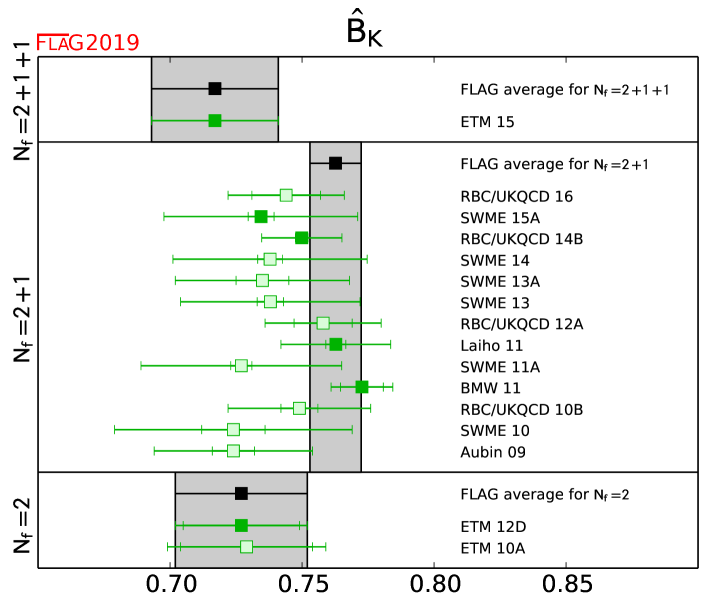
Figure 18: Recent unquenched lattice results for the RGI $B$-parameter $\hat{B}_{K}$. The grey bands indicate our global averages described in the text. For $N_{f}=2+1+1$ and $N_{f}=2$ the global estimate coincide with the results by ETM 12D and ETM 10A, respectively.

Passing over to describing the results computed for $N_{f}=2$ flavours, we note that there is only the set of results published in ETM 12D [Bertone:2012cu] and ETM 10A [Constantinou:2010qv] that allow for an extensive investigation of systematic uncertainties. We identify the result from ETM 12D [Bertone:2012cu], which is an update of ETM 10A, with the currently best global estimate for two-flavour QCD, i.e.,

$$N_{f}=2:\hskip 8.5359pt\hat{B}_{K}=0.727(22)(12),\hskip 8.5359ptB_{K}^{\overline{\mathrm{MS}}}(2\,{\rm GeV})=0.531(16)(19)\hskip 11.38092pt\ref{~}\mbox{\cite[cite]{[\@@bibref{Number}{Bertone:2012cu}{}{}]}}.$$ (152)

The result in the ${\overline{\mathrm{MS}}}$ scheme has been obtained by applying the same conversion factor of 1.369 as in the three-flavour theory.

6.3 Kaon BSM $B$-parameters

We now report on lattice results concerning the matrix elements of operators that encode the effects of physics beyond the Standard Model (BSM) to the mixing of neutral kaons. In this theoretical framework both the SM and BSM contributions add up to reproduce the experimentally observed value of $\epsilon_{K}$. Since BSM contributions involve heavy but unobserved particles they are short-distance dominated. The effective Hamiltonian for generic ${\Delta}S=2$ processes including BSM contributions reads

$${\cal H}_{\rm eff,BSM}^{\Delta S=2}=\sum_{i=1}^{5}C_{i}(\mu)Q_{i}(\mu),$$ (153)

where $Q_{1}$ is the four-quark operator of Eq. (136) that gives rise to the SM contribution to $\epsilon_{K}$. In the so-called SUSY basis introduced by Gabbiani et al. [Gabbiani:1996hi] the operators $Q_{2},\ldots,Q_{5}$ read 

$$Q_{2}={\hbox{$\left(\vbox to0.0pt{}\right.\n@space$}}\bar{s}^{a}(1-\gamma_{5})d^{a}{\hbox{$\left)\vbox to0.0pt{}\right.\n@space$}}{\hbox{$\left(\vbox to0.0pt{}\right.\n@space$}}\bar{s}^{b}(1-\gamma_{5})d^{b}{\hbox{$\left)\vbox to0.0pt{}\right.\n@space$}},$$

$$Q_{3}={\hbox{$\left(\vbox to0.0pt{}\right.\n@space$}}\bar{s}^{a}(1-\gamma_{5})d^{b}{\hbox{$\left)\vbox to0.0pt{}\right.\n@space$}}{\hbox{$\left(\vbox to0.0pt{}\right.\n@space$}}\bar{s}^{b}(1-\gamma_{5})d^{a}{\hbox{$\left)\vbox to0.0pt{}\right.\n@space$}},$$

$$Q_{4}={\hbox{$\left(\vbox to0.0pt{}\right.\n@space$}}\bar{s}^{a}(1-\gamma_{5})d^{a}{\hbox{$\left)\vbox to0.0pt{}\right.\n@space$}}{\hbox{$\left(\vbox to0.0pt{}\right.\n@space$}}\bar{s}^{b}(1+\gamma_{5})d^{b}{\hbox{$\left)\vbox to0.0pt{}\right.\n@space$}},$$

$$Q_{5}={\hbox{$\left(\vbox to0.0pt{}\right.\n@space$}}\bar{s}^{a}(1-\gamma_{5})d^{b}{\hbox{$\left)\vbox to0.0pt{}\right.\n@space$}}{\hbox{$\left(\vbox to0.0pt{}\right.\n@space$}}\bar{s}^{b}(1+\gamma_{5})d^{a}{\hbox{$\left)\vbox to0.0pt{}\right.\n@space$}},$$ (154)

where $a$ and $b$ denote colour indices. In analogy to the case of $B_{K}$ one then defines the $B$-parameters of $Q_{2},\ldots,Q_{5}$ according to

$$B_{i}(\mu)=\frac{\left\langle\bar{K}^{0}\left|Q_{i}(\mu)\right|K^{0}\right\rangle}{N_{i}\left\langle\bar{K}^{0}\left|\bar{s}\gamma_{5}d\right|0\right\rangle\left\langle 0\left|\bar{s}\gamma_{5}d\right|K^{0}\right\rangle},\quad i=2,\ldots,5.$$ (155)

The factors $\{N_{2},\ldots,N_{5}\}$ are given by $\{-5/3,1/3,2,2/3\}$, and it is understood that $B_{i}(\mu)$ is specified in some renormalization scheme, such as ${\overline{\mathrm{MS}}}$ or a variant of the regularization-independent momentum subtraction (RI-MOM) scheme.

The SUSY basis has been adopted in Refs. [Boyle:2012qb, Bertone:2012cu, Carrasco:2015pra, Garron:2016mva]. Alternatively, one can employ the chiral basis of Buras, Misiak and Urban [Buras:2000if]. The SWME collaboration prefers the latter since the anomalous dimension that enters the RG running has been calculated to two loops in perturbation theory [Buras:2000if]. Results obtained in the chiral basis can be easily converted to the SUSY basis via

$$B_{3}^{\rm SUSY}={\textstyle\frac{1}{2}}\left(5B_{2}^{\rm chiral}-3B_{3}^{\rm chiral}\right).$$ (156)

The remaining $B$-parameters are the same in both bases. In the following we adopt the SUSY basis and drop the superscript.

Older quenched results for the BSM $B$-parameters can be found in Refs. [Allton:1998sm, Donini:1999nn, Babich:2006bh]. For a nonlattice approach to get estimates for the BSM $B$-parameters see Ref. [Buras:2018lgu].

Estimates for $B_{2},\ldots,B_{5}$ have been reported for QCD with $N_{f}=2$ (ETM 12D [Bertone:2012cu]), $N_{f}=2+1$ (RBC/UKQCD 12E [Boyle:2012qb], SWME 13A [Bae:2013tca], SWME 14C [Jang:2014aea], SWME 15A [Jang:2015sla], RBC/UKQCD 16 [Garron:2016mva, Boyle:2017skn]) and $N_{f}=2+1+1$ (ETM 15 [Carrasco:2015pra]) flavours of dynamical quarks. They are listed and compared in Tab. 1 and Fig. 19. In general one finds that the BSM $B$-parameters computed by different collaborations do not show the same level of consistency as the SM kaon mixing parameter $B_{K}$ discussed previously. Control over systematic uncertainties (chiral and continuum extrapolations, finite-volume effects) in $B_{2},\ldots,B_{5}$ is expected to be at the same level as for $B_{K}$, as far as the results by ETM 12D, ETM 15 and SWME 15A are concerned. The calculation by RBC/UKQCD 12E has been performed at a single value of the lattice spacing and a minimum pion mass of 290 MeV. Thus, the results do not benefit from the same improvements regarding control over the chiral and continuum extrapolations as in the case of $B_{K}$ [Blum:2014tka].

The RBC/UKQCD collaboration has recently extended its calculation of BSM $B$-parameters [Garron:2016mva, Boyle:2017skn] for $N_{f}=2+1$, by considering two values of the lattice spacing, $a\simeq 0.11$ and 0.08 fm, employing ensembles generated using the Iwasaki gauge action and the Shamir domain-wall fermionic action. The lattice volumes in the RBC/UKQCD 16 calculation are $24^{3}\times 64\times 16$ for the coarse and $32^{3}\times 64\times 16$ for the fine lattice spacing, while the lowest simulated values for the pseudoscalar mass are about 340 MeV and 300 MeV, respectively. As in the related calculation of $B_{K}$ (RBC/UKQCD 14B [Blum:2014tka]) the renormalization of four-quark operators was performed nonperturbatively in two RI-SMOM schemes, namely, $({\mathchoice{\c@ncel\displaystyle{q}}{\c@ncel\textstyle{q}}{\c@ncel\scriptstyle{q}}{\c@ncel\scriptscriptstyle{q}}},{\mathchoice{\c@ncel\displaystyle{q}}{\c@ncel\textstyle{q}}{\c@ncel\scriptstyle{q}}{\c@ncel\scriptscriptstyle{q}}})$ and $(\gamma_{\mu},\gamma_{\mu})$, where the latter was used for the final estimates of $B_{2},\ldots,B_{5}$ quoted in Ref. [Garron:2016mva]. By comparing the results obtained in the conventional RI-MOM and the two RI-SMOM schemes, RBC/UKQCD 16 report significant discrepancies for $B_{4}$ and $B_{5}$ in the $\overline{\rm{MS}}$ scheme at the scale of 3 GeV, which amount up to 2.8$\sigma$ in the case of $B_{5}$. By contrast, the agreement for $B_{2}$ and $B_{3}$ determined for different intermediate scheme is much better. Based on these findings they claim that these discrepancies are due to uncontrolled systematics coming from the Goldstone boson pole subtraction procedure that is needed in the RI-MOM scheme, while pole subtraction effects are much suppressed in RI-SMOM thanks to the fact that the latter is based on nonexceptional momenta. The RBC/UKQCD collaboration has presented an ongoing study [Boyle:2018eor] in which simulations with two values of the lattice spacing at the physical point and with a third finer lattice spacing at $M_{\pi}=234$ MeV are employed in order to obtain the BSM matrix elements in the continuum limit. Results are still preliminary.

The findings by RBC/UKQCD 16 [Garron:2016mva, Boyle:2017skn] provide evidence that the nonperturbative determination of the matching factors depends strongly on the details of the implementation of the Rome-Southampton method. The use of nonexceptional momentum configurations in the calculation of the vertex functions produces a significant modification of the renormalization factors, which affects the matching between $\overline{\rm{MS}}$ and the intermediate momentum subtraction scheme. This effect is most pronounced in $B_{4}$ and $B_{5}$. Furthermore, it can be noticed that the estimates for $B_{4}$ and $B_{5}$ from RBC/UKQCD 16 are much closer to those of SWME 15A. At the same time, the results for $B_{2}$ and $B_{3}$ obtained by ETM 15, SWME 15A and RBC/UKQCD 16 are in good agreement within errors.

Collaboration	Ref.	$N_{f}$	publication status	continuum extrapolation	chiral extrapolation	finite volume	renormalization	running	$B_{2}$	$B_{3}$	$B_{4}$	$B_{5}$
ETM 15	[Carrasco:2015pra]	2+1+1	A	$\bigstar$	$\circ$	$\circ$	$\bigstar$	$\,a$	0.46(1)(3)	0.79(2)(5)	0.78(2)(4)	0.49(3)(3)
RBC/UKQCD 16	[Garron:2016mva]	2+1	A	$\circ$	$\circ$	$\circ$	$\bigstar$	$\,b$	0.488(7)(17)	0.743(14)(65)	0.920(12)(16)	0.707(8)(44)
SWME 15A	[Jang:2015sla]	2+1	A	$\bigstar$	$\circ$	$\bigstar$	$\circ$${}^{\dagger}$	$-$	0.525(1)(23)	0.773(6)(35)	0.981(3)(62)	0.751(7)(68)
SWME 14C	[Jang:2014aea]	2+1	C	$\bigstar$	$\circ$	$\bigstar$	$\circ$${}^{\dagger}$	$-$	0.525(1)(23)	0.774(6)(64)	0.981(3)(61)	0.748(9)(79)
SWME 13A${}^{\ddagger}$	[Bae:2013tca]	2+1	A	$\bigstar$	$\circ$	$\bigstar$	$\circ$${}^{\dagger}$	$-$	0.549(3)(28)	0.790(30)	1.033(6)(46)	0.855(6)(43)
RBC/	[Boyle:2012qb]	2+1	A	$\blacksquare$	$\circ$	$\bigstar$	$\bigstar$	$\,b$	0.43(1)(5)	0.75(2)(9)	0.69(1)(7)	0.47(1)(6)
UKQCD 12E
ETM 12D	[Bertone:2012cu]	2	A	$\bigstar$	$\circ$	$\circ$	$\bigstar$	$\,c$	0.47(2)(1)	0.78(4)(2)	0.76(2)(2)	0.58(2)(2)

• The renormalization is performed using perturbation theory at one loop, with a conservative estimate of the uncertainty.
  

• $B_{i}$ are renormalized nonperturbatively at scales $1/a\sim 2.2-3.3\,\mathrm{Ge\kern-0.80005ptV}$ in the $N_{f}=4$ RI/MOM scheme using two different lattice momentum scale intervals, with values around $1/a$ for the first and around 3.5 GeV for the second one. The impact of these two ways to the final result is taken into account in the error budget. Conversion to ${\overline{\mathrm{MS}}}$ is at one loop at 3 GeV.
  

• The $B$-parameters are renormalized nonperturbatively at a scale of 3 GeV.
  

• $B_{i}$ are renormalized nonperturbatively at scales $1/a\sim 2-3.7\,\mathrm{Ge\kern-0.80005ptV}$ in the $N_{f}=2$ RI/MOM scheme using two different lattice momentum scale intervals, with values around $1/a$ for the first and around 3 GeV for the second one.
  

• The computation of $B_{4}$ and $B_{5}$ has been revised in Refs. [Jang:2015sla] and [Jang:2014aea].

Table 29: Results for the BSM $B$-parameters $B_{2},\ldots,B_{5}$ in the ${\overline{\mathrm{MS}}}$ scheme at a reference scale of 3 GeV. Any available information on nonperturbative running is indicated in the column “running”, with details given at the bottom of the table. 

A nonperturbative computation of the running of the four-fermion operators contributing to the $B_{2}$, …, $B_{5}$ parameters has been carried out with two dynamical flavours using the Schrödinger functional renormalization scheme [Dimopoulos:2018zef]. Renormalization matrices of the operator basis are used to build step-scaling functions governing the continuum-limit running between hadronic and electroweak scales. A comparison to perturbative results using NLO (2-loops) for the four-fermion operator anomalous dimensions indicates that, at scales of about 3 GeV, nonperturbative effects can induce a sizeable contribution to the running.

A detailed look at the most recent calculations reported in ETM 15 [Carrasco:2015pra], SWME 15A [Jang:2015sla] and RBC/UKQCD 16 [Garron:2016mva] reveals that cutoff effects appear to be larger for the BSM $B$-parameters compared to $B_{K}$. Depending on the details of the renormalization procedure and/or the fit ansatz for the combined chiral and continuum extrapolation, the results obtained at the coarsest lattice spacing differ by 15–30%. At the same time the available range of lattice spacings is typically much reduced compared to the corresponding calculations of $B_{K}$, as can be seen by comparing the quality criteria in Tabs. 1 and 1. Hence, the impact of the renormalization procedure and the continuum limit on the BSM $B$-parameters certainly requires further investigation.

Finally we present our estimates for the BSM $B$-parameters, quoted in the ${\overline{\mathrm{MS}}}$-scheme at scale 3 GeV. For $N_{f}=2+1$ our estimate is given by the average between the results from SWME 15A and RBC/UKQCD 16, i.e.,

$$N_{f}=2+1:$$ (157)

$$B_{2}=0.502(14),\quad B_{3}=0.766(32),\quad B_{4}=0.926(19),\quad B_{5}=0.720(38),\quad\,\mathrm{Refs.}~{}\mbox{\cite[cite]{[\@@bibref{Number}{Jang:2015sla,Garron:2016mva}{}{}]}}.$$

For $N_{f}=2+1+1$ and $N_{f}=2$, our estimates coincide with the ones by ETM 15 and ETM 12D, respectively, since there is only one computation for each case. Thus we quote

$$N_{f}=2+1+1:$$ (158)

$$B_{2}=0.46(1)(3),\quad B_{3}=0.79(2)(4),\quad B_{4}=0.78(2)(4),\quad B_{5}=0.49(3)(3),\quad\ref{~}\mbox{\cite[cite]{[\@@bibref{Number}{Carrasco:2015pra}{}{}]}},$$

$$N_{f}=2:$$ (159)

$$B_{2}=0.47(2)(1),\quad B_{3}=0.78(4)(2),\quad B_{4}=0.76(2)(2),\quad B_{5}=0.58(2)(2),\quad\ref{~}\mbox{\cite[cite]{[\@@bibref{Number}{Bertone:2012cu}{}{}]}}.$$

Based on the above discussion on the effects of employing different intermediate momentum subtraction schemes in the nonperturbative renormalization of the operators, the discrepancy for $B_{4}$ and $B_{5}$ results between $N_{f}=2,2+1+1$ and $N_{f}=2+1$ computations should not be considered an effect associated with the number of dynamical flavours. As a closing remark, we encourage authors to provide the correlation matrix of the $B_{i}$ parameters.

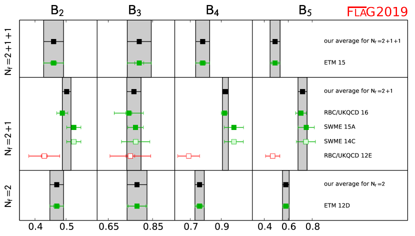
Figure 19: Lattice results for the BSM $B$-parameters defined in the ${\overline{\mathrm{MS}}}$ scheme at a reference scale of 3 GeV, see Tab. 1.

7 $D$-meson decay constants and form factors

Authors: Y. Aoki, D. Bečirević, M. Della Morte, S. Gottlieb, D. Lin, E. Lunghi, C. Pena

Leptonic and semileptonic decays of charmed $D$ and $D_{s}$ mesons occur via charged $W$-boson exchange, and are sensitive probes of $c\to d$ and $c\to s$ quark flavour-changing transitions. Given experimental measurements of the branching fractions combined with sufficiently precise theoretical calculations of the hadronic matrix elements, they enable the determination of the CKM matrix elements $|V_{cd}|$ and $|V_{cs}|$ (within the Standard Model) and a precise test of the unitarity of the second row of the CKM matrix. Here we summarize the status of lattice-QCD calculations of the charmed leptonic decay constants. Significant progress has been made in charm physics on the lattice in recent years, largely due to the availability of gauge configurations produced using highly-improved lattice-fermion actions that enable treating the $c$ quark with the same action as for the $u$, $d$, and $s$ quarks.

This section updates the corresponding one in the last FLAG review [Aoki:2016frl] for results that appeared after November 30, 2015. As already done in Ref. [Aoki:2016frl], we limit our review to results based on modern simulations with reasonably light pion masses (below approximately 500 MeV). This excludes results obtained from the earliest unquenched simulations, which typically had two flavours in the sea, and which were limited to heavier pion masses because of the constraints imposed by the computational resources and methods available at that time.

Following our review of lattice-QCD calculations of $D_{(s)}$-meson leptonic decay constants and semileptonic form factors, we then interpret our results within the context of the Standard Model. We combine our best-determined values of the hadronic matrix elements with the most recent experimentally-measured branching fractions to obtain $|V_{cd(s)}|$ and test the unitarity of the second row of the CKM matrix.

7.1 Leptonic decay constants $f_{D}$ and $f_{D_{s}}$

In the Standard Model, and up to electromagnetic corrections, the decay constant $f_{D_{(s)}}$ of a pseudoscalar $D$ or $D_{s}$ meson is related to the branching ratio for leptonic decays mediated by a $W$ boson through the formula

$${\mathcal{B}}(D_{(s)}\to\ell\nu_{\ell})={{G_{F}^{2}|V_{cq}|^{2}\tau_{D_{(s)}}}\over{8\pi}}f_{D_{(s)}}^{2}m_{\ell}^{2}m_{D_{(s)}}\left(1-{{m_{\ell}^{2}}\over{m_{D_{(s)}}^{2}}}\right)^{2}\;,$$ (160)

where $q$ is $d$ or $s$ and $V_{cd}$ ($V_{cs}$) is the appropriate CKM matrix element for a $D$ ($D_{s}$) meson. The branching fractions have been experimentally measured by CLEO, Belle, Babar and BES with a precision around 4–5$\%$ for both the $D$ and the $D_{s}$-meson decay modes [Rosner:2015wva]. When combined with lattice results for the decay constants, they allow for determinations of $|V_{cs}|$ and $|V_{cd}|$.

In lattice-QCD calculations the decay constants $f_{D_{(s)}}$ are extracted from Euclidean matrix elements of the axial current

$$\langle 0|A^{\mu}_{cq}|D_{q}(p)\rangle=if_{D_{q}}\;p_{D_{q}}^{\mu}\;,$$ (161)

with $q=d,s$ and $A^{\mu}_{cq}=\bar{c}\gamma_{\mu}\gamma_{5}q$. Results for $N_{f}=2,\;2+1$ and $2+1+1$ dynamical flavours are summarized in Tab. 1 and Fig. 20. Since the publication of the last FLAG review, a handful of results for $f_{D}$ and $f_{D_{s}}$ have appeared, as described below. We consider isospin-averaged quantities, although in a few cases results for $f_{D^{+}}$ are quoted (see, for example, the FNAL/MILC 11,14A and 17 computations, where the difference between $f_{D}$ and $f_{D^{+}}$ has been estimated to be around 0.5 MeV).

One new result has appeared for $N_{f}=2$. Blossier 18 [Blossier:2018jol] employs a subset of the gauge field configuration ensembles entering the earlier study presented in ALPHA 13B [Heitger:2013oaa] by the ALPHA collaboration, however, it is independent of it; in particular, in [Blossier:2018jol] a different strategy is used to analyse the raw data, based on matrices of correlation functions and by solving a Generalized Eigenvalue Problem. It describes a determination of the $D_{s}$ and $D_{s}^{*}$ decay constants computed on six $N_{f}=2$ ensembles of nonperturbatively O($a$) improved Wilson fermions at lattice spacings of 0.065 and 0.048 fm. Pion masses range between 440 and 194 MeV and the condition $Lm_{\pi}\geq 4$ is always met. Chiral/continuum extrapolations are performed adopting a fit ansatz linear in $m_{\pi}^{2}$ and $a^{2}$. The systematic errors are dominated by the uncertainty on the absolute lattice scale, which is fixed through $f_{K}$. Cutoff effects on $f_{D_{s}}$ instead appear to be small and are at the 1% level at the coarsest lattice spacing.

Collaboration	Ref.	$N_{f}$	publication status	continuum extrapolation	chiral extrapolation	finite volume	renormalization/matching	heavy-quark treatment	$f_{D}$	$f_{D_{s}}$	$f_{D_{s}}/f_{D}$
FNAL/MILC 17 ${}^{\nabla\nabla}$	[Bazavov:2017lyh]	2+1+1	A	$\bigstar$	$\bigstar$	$\bigstar$	$\bigstar$	✓	212.1(0.6)	249.9(0.5)	1.1782(16)
FNAL/MILC 14A${}^{**}$	[Bazavov:2014wgs]	2+1+1	A	$\bigstar$	$\bigstar$	$\bigstar$	$\bigstar$	✓	212.6(0.4) $+1.0\choose-1.2$	249.0(0.3)$+1.1\choose-1.5$	1.1745(10)$+29\choose-32$
ETM 14E${}^{\dagger}$	[Carrasco:2014poa]	2+1+1	A	$\bigstar$	$\circ$	$\circ$	$\bigstar$	✓	207.4(3.8)	247.2(4.1)	1.192(22)
ETM 13F	[Dimopoulos:2013qfa]	2+1+1	C	$\circ$	$\circ$	$\circ$	$\bigstar$	✓	202(8)	242(8)	1.199(25)
FNAL/MILC 13${}^{\nabla}$	[Bazavov:2013nfa]	2+1+1	C	$\bigstar$	$\bigstar$	$\bigstar$	$\bigstar$	✓	212.3(0.3)(1.0)	248.7(0.2)(1.0)	1.1714(10)(25)
FNAL/MILC 12B	[Bazavov:2012dg]	2+1+1	C	$\bigstar$	$\bigstar$	$\bigstar$	$\bigstar$	✓	209.2(3.0)(3.6)	246.4(0.5)(3.6)	1.175(16)(11)
RBC/UKQCD 17	[Boyle:2017jwu]	2+1	A	$\bigstar$	$\bigstar$	$\circ$	$\bigstar$	✓	208.7(2.8)$+2.1\choose-1.8$	246.4(1.3)$+1.3\choose-1.9$	1.1667(77)$+57\choose-43$
$\chi$QCD 14	[Yang:2014sea]	2+1	A	$\circ$	$\circ$	$\circ$	$\bigstar$	✓		254(2)(4)
HPQCD 12A	[Na:2012iu]	2+1	A	$\circ$	$\circ$	$\circ$	$\bigstar$	✓	208.3(1.0)(3.3)	246.0(0.7)(3.5)	1.187(4)(12)
FNAL/MILC 11	[Bazavov:2011aa]	2+1	A	$\circ$	$\circ$	$\circ$	$\circ$	✓	218.9(11.3)	260.1(10.8)	1.188(25)
PACS-CS 11	[Namekawa:2011wt]	2+1	A	$\blacksquare$	$\bigstar$	$\blacksquare$	$\circ$	✓	226(6)(1)(5)	257(2)(1)(5)	1.14(3)
HPQCD 10A	[Davies:2010ip]	2+1	A	$\bigstar$	$\circ$	$\bigstar$	$\bigstar$	✓	213(4)${}^{*}$	248.0(2.5)
HPQCD/UKQCD 07	[Follana:2007uv]	2+1	A	$\bigstar$	$\circ$	$\circ$	$\bigstar$	✓	207(4)	241 (3)	1.164(11)
FNAL/MILC 05	[Aubin:2005ar]	2+1	A	$\circ$	$\circ$	$\blacksquare$	$\circ$	✓	201(3)(17)	249(3)(16)	1.24(1)(7)
Blossier 18	[Blossier:2018jol]	2	A	$\circ$	$\bigstar$	$\circ$	$\bigstar$	✓		238(5)(2)
TWQCD 14${}^{\square\square}$	[Chen:2014hva]	2	A	$\blacksquare$	$\circ$	$\blacksquare$	$\bigstar$	✓	202.3(2.2)(2.6)	258.7(1.1)(2.9)	1.2788(264)
ALPHA 13B	[Heitger:2013oaa]	2	C	$\circ$	$\bigstar$	$\circ$	$\bigstar$	✓	216(7)(5)	247(5)(5)	1.14(2)(3)
ETM 13B${}^{\square}$	[Carrasco:2013zta]	2	A	$\bigstar$	$\circ$	$\circ$	$\bigstar$	✓	208(7)	250(7)	1.20(2)
ETM 11A	[Dimopoulos:2011gx]	2	A	$\bigstar$	$\circ$	$\circ$	$\bigstar$	✓	212(8)	248(6)	1.17(5)
ETM 09	[Blossier:2009bx]	2	A	$\circ$	$\circ$	$\circ$	$\bigstar$	✓	197(9)	244(8)	1.24(3)

${}^{\dagger}$ Update of ETM 13F
${}^{\nabla}$ Update of FNAL/MILC 12B.
${}^{*}$ This result is obtained by using the central value for $f_{D_{s}}/f_{D}$ from HPQCD/UKQCD 07 and increasing the error to account for the effects from the change in the physical value of $r_{1}$.
${}^{\square}$ Update of ETM 11A and ETM 09.
${}^{\square\square}$ One lattice spacing $\simeq 0.1$ fm only. $m_{\pi,{\rm min}}L=1.93$.
${}^{**}$ At $\beta=5.8$, $m_{\pi,\rm min}L=3.2$ but this lattice spacing is not used in the final cont./chiral extrapolations.
${}^{\nabla\nabla}$ Update of FNAL/MILC 14A. The ratio quoted is $f_{D_{s}}/f_{D^{+}}=1.1749(16)$. In order to compare with results from other collaborations we rescale the number by the ratio of central values for $f_{D+}$ and $f_{D}$. We use the same rescaling in FNAL/MILC 14A. At the finest lattice spacing the finite-volume criterium would produce an empty green circle, however, as checked by the authors, results would not significantly change by excluding this ensemble, which instead sharpens the continuum limit extrapolation.

Table 30: Decay constants of the $D$ and $D_{s}$ mesons (in MeV) and their ratio.

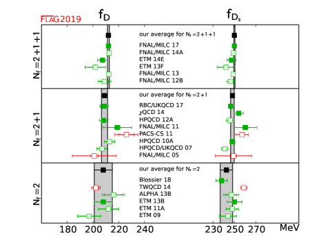
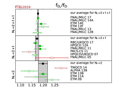
Figure 20: Decay constants of the $D$ and $D_{s}$ mesons [values in Tab. 1 and Eqs. (162-170)]. As usual, full green squares are used in the averaging procedure, pale green squares have been superseded by later determinations, while pale red squares do not satisfy the criteria. The black squares and grey bands indicate our averages.

The $N_{f}=2$ averages for $f_{D}$ and ${{f_{D_{s}}}/{f_{D}}}$ coincide with those in the previous FLAG review and are given by the values in ETM 13B [Carrasco:2013zta], while the estimate for $f_{D_{s}}$ is the result of the weighted average of the numbers in ETM 13B [Carrasco:2013zta] and Blossier 18 [Blossier:2018jol]. They read

$$N_{f}=2: f_{D} =208(7)\;{\rm MeV} \ref{~}\mbox{\cite[cite]{[\@@bibref{Number}{Carrasco:2013zta}{}{}]}},$$ (162)

$$N_{f}=2: f_{D_{s}} =242.5(5.8)\;{\rm MeV} \,\mathrm{Refs.}~{}\mbox{\cite[cite]{[\@@bibref{Number}{Carrasco:2013zta,Blossier:2018jol}{}{}]}},$$ (163)

$$N_{f}=2: f_{D_{s}}\over{f_{D}} =1.20(0.02) \ref{~}\mbox{\cite[cite]{[\@@bibref{Number}{Carrasco:2013zta}{}{}]}},$$ (164)

where the error on the average of $f_{D_{s}}$ has been rescaled by the factor $\sqrt{\chi^{2}/\mbox{dof}}=1.34$ (see Sec. 2).

The RBC/UKQCD collaboration presented in RBC/UKQCD 17 [Boyle:2017jwu] the final results for the computation of the $D$- and $D_{s}$-mesons decay constants based on the $N_{f}=2+1$ dynamical ensembles generated using Domain Wall Fermions (DWF). Three lattice spacings have been considered with pion masses ranging between the physical value (reached at the two coarsest lattice spacings) and 430 MeV. Two different Domain Wall discretizations (Möbius and Shamir) have been used for both (light) valence and sea quarks. They correspond to two different choices for the DWF kernel. The Möbius DWF are loosely equivalent to Shamir DWF at twice the extension in the fifth dimension [Blum:2014tka]. For the actual implementation by the RBC/UKQCD collaboration O$(a^{2})$ cutoff effects in the two formulations are expected to agree and results are therefore extrapolated jointly to the continuum limit. For the quenched charm quark Möbius DWF are always used, with a domain-wall height slightly different from the one adopted for light valence quarks. The choice helps to keep cutoff effects under control, according to the study in Ref. [Boyle:2016imm]. The continuum/physical-mass extrapolations are performed by using a Taylor expansion in $a^{2}$ and $m_{\pi}^{2}-m_{\pi}^{2\,phys}$ and the associated systematic error is estimated by essentially applying cuts in the pion mass. This error dominates the uncertainties on the final results.

The updated FLAG estimates then read

$$N_{f}=2+1: f_{D} =209.0(2.4)\;{\rm MeV} \,\mathrm{Refs.}~{}\mbox{\cite[cite]{[\@@bibref{Number}{Na:2012iu,Bazavov:2011aa,Boyle:2017jwu}{}{}]}},$$ (165)

$$N_{f}=2+1: f_{D_{s}} =248.0(1.6)\;{\rm MeV} \,\mathrm{Refs.}~{}\mbox{\cite[cite]{[\@@bibref{Number}{Davies:2010ip,Bazavov:2011aa,Boyle:2017jwu,Yang:2014sea}{}{}]}},$$ (166)

$$N_{f}=2+1: f_{D_{s}}\over{f_{D}} =1.174(0.007) \,\mathrm{Refs.}~{}\mbox{\cite[cite]{[\@@bibref{Number}{Na:2012iu,Bazavov:2011aa,Boyle:2017jwu}{}{}]}},$$ (167)

where the error on the $N_{f}=2+1$ average of $f_{D_{s}}$ has been rescaled by the factor $\sqrt{\chi^{2}/\mbox{dof}}=1.1$. Those come from the results in HPQCD 12A [Na:2012iu], FNAL/MILC 11 [Bazavov:2011aa] as well as RBC/UKQCD 17 [Boyle:2017jwu] concerning $f_{D}$ while for $f_{D_{s}}$ also the $\chi$QCD 14 [Yang:2014sea] result contributes, and instead of the value in HPQCD 12A [Na:2012iu] the one in HPQCD 10A [Davies:2010ip] is used. In addition, the statistical errors between the results of FNAL/MILC and HPQCD have been everywhere treated as 100% correlated since the two collaborations use overlapping sets of configurations. The same procedure had been used in the past reviews.

For $N_{f}=2+1+1$ one new determination (FNAL/MILC 17) appeared in [Bazavov:2017lyh], which is actually an extension of FNAL/MILC 14A [Bazavov:2014wgs] (described in detail in the previous FLAG review). While in FNAL/MILC 14A the finest lattice spacing considered was 0.06 fm, in FNAL/MILC 17 three new ensembles have been employed; two with resolution 0.042 fm and light-quark masses equal to either one fifth of the strange-quark mass ($m_{s}/5$) or to the physical up-down average mass, and one at $a\approx$ 0.03 fm with light-quark masses equal to $m_{s}/5$. In addition, the statistics on the $a\approx$ 0.06 fm ensemble have been increased. As in FNAL/MILC 14A, the HISQ fermionic regularization and the 1-loop tadpole improved Symanzik gauge action have been used for the generation of configurations, produced by a combination of the RHMC and the RHMD algorithms. The analysis, absolute and relative scale setting, and the chiral/continuum extrapolations are performed in essentially the same way as in FNAL/MILC 14A and the latter rely on the use of heavy-meson rooted all-staggered chiral perturbation theory (HMrAS$\chi$PT) [Bernard:2013qwa] at NNLO with the inclusion of N${}^{3}$LO mass-dependent analytic terms. A novel aspect is represented by the inclusion of corrections due to the nonequilibration of the topological charge. Such freezing of the topology is particularly severe at the two new fine lattice spacings. Following [Bernard:2017npd] such corrections are computed in the context of heavy-meson $\chi$PT, through an expansion in $1/\chi_{T}V$, with $\chi_{T}$ being the topological susceptibility in a fully-sampled, large-volume ensemble. The resulting systematic error turns out to be of the same size as other systematic uncertainties such as the scale setting. The final total errors (below 0.5%) however are dominated by statistics and the systematic due to chiral/continuum extrapolations. As in FNAL/MILC 14A the results for the decay constants are used in combination with the experimental decay rates for $D_{(s)}^{+}\to\ell\nu_{\ell}$ in order to perform a unitarity test of the second row of the CKM matrix. After correcting the experimental decay rates from PDG by the known long- and short-distance electroweak contributions and including a 0.6% uncertainty to account for unknown electromagnetic corrections (as done in FNAL/MILC 14A and discussed in the previous FLAG review), the FNAL/MILC collaboration obtains $1-|V_{cd}|^{2}-|V_{cs}|^{2}-|V_{cb}|^{2}=-0.049(32)$, which is compatible with CKM unitarity within 1.5 standard deviations.

The results in FNAL/MILC 17 [Bazavov:2017lyh] replace those from FNAL/MILC 14A [Bazavov:2014wgs] in our $N_{f}=2+1+1$ final estimates, which are therefore obtained by performing a weighted average with ETM 14E [Carrasco:2014poa] and read

$$N_{f}=2+1+1: f_{D} =212.0(0.7)\;{\rm MeV} \,\mathrm{Refs.}~{}\mbox{\cite[cite]{[\@@bibref{Number}{Bazavov:2017lyh,Carrasco:2014poa}{}{}]}},$$ (168)

$$N_{f}=2+1+1: f_{D_{s}} =249.9(0.5)\;{\rm MeV} \,\mathrm{Refs.}~{}\mbox{\cite[cite]{[\@@bibref{Number}{Bazavov:2017lyh,Carrasco:2014poa}{}{}]}},$$ (169)

$$N_{f}=2+1+1: f_{D_{s}}\over{f_{D}} =1.1783(0.0016) \,\mathrm{Refs.}~{}\mbox{\cite[cite]{[\@@bibref{Number}{Bazavov:2017lyh,Carrasco:2014poa}{}{}]}},$$ (170)

where the error on the average of $f_{D}$ has been rescaled by the factor $\sqrt{\chi^{2}/\mbox{dof}}=1.22$.

7.2 Form factors for $D\to\pi\ell\nu$ and $D\to K\ell\nu$ semileptonic decays

The SM prediction for the differential decay rate of the semileptonic processes $D\to\pi\ell\nu$ and $D\to K\ell\nu$ can be written as

$$\hbox{$d\Gamma(D\to P\ell\nu)\over dq^{2}$}=\hbox{$G_{\rm\scriptscriptstyle F}^{2}|V_{cx}|^{2}\over 24\pi^{3}$}\,\hbox{$(q^{2}-m_{\ell}^{2})^{2}\sqrt{E_{P}^{2}-m_{P}^{2}}\over q^{4}m_{D}^{2}$}\,{\hbox{$\left[\vbox to0.0pt{}\right.\n@space$}}\left(1+\hbox{$m_{\ell}^{2}\over 2q^{2}$}\right)m_{D}^{2}(E_{P}^{2}-m_{P}^{2})|f_{+}(q^{2})|^{2}$$

$$+\hbox{$3m_{\ell}^{2}\over 8q^{2}$}(m_{D}^{2}-m_{P}^{2})^{2}|f_{0}(q^{2})|^{2} \!\!\!\!{\hbox{$\left]\vbox to0.0pt{}\right.\n@space$}}\,,$$ (171)

where $x=d,s$ is the daughter light quark, $P=\pi,K$ is the daughter light-pseudoscalar meson, $q=(p_{D}-p_{P})$ is the momentum of the outgoing lepton pair, and $E_{P}$ is the light-pseudoscalar meson energy in the rest frame of the decaying $D$. The vector and scalar form factors $f_{+}(q^{2})$ and $f_{0}(q^{2})$ parameterize the hadronic matrix element of the heavy-to-light quark flavour-changing vector current $V_{\mu}=\overline{x}\gamma_{\mu}c$,

$$\langle P|V_{\mu}|D\rangle=f_{+}(q^{2})\left({p_{D}}_{\mu}+{p_{P}}_{\mu}-\hbox{$m_{D}^{2}-m_{P}^{2}\over q^{2}$}\,q_{\mu}\right)+f_{0}(q^{2})\hbox{$m_{D}^{2}-m_{P}^{2}\over q^{2}$}\,q_{\mu}\,,$$ (172)

and satisfy the kinematic constraint $f_{+}(0)=f_{0}(0)$. Because the contribution to the decay width from the scalar form factor is proportional to $m_{\ell}^{2}$, within current precision standards it can be neglected for $\ell=e,\mu$, and Eq. (171) simplifies to

$$\hbox{$d\Gamma\!\left(D\to P\ell\nu\right)\over dq^{2}$}=\hbox{$G_{\rm\scriptscriptstyle F}^{2}\over 24\pi^{3}$}|\vec{p}_{P}|^{3}{|V_{cx}|^{2}|f_{+}(q^{2})|^{2}}\,.$$ (173)

In models of new physics, decay rates may also receive contributions from matrix elements of other parity-even currents. In the case of the scalar density, partial vector current conservation allows one to write matrix elements of the latter in terms of $f_{+}$ and $f_{0}$, while for tensor currents $T_{\mu\nu}=\bar{x}\sigma_{\mu\nu}c$ a new form factor has to be introduced, viz.,

$$\langle P|T_{\mu\nu}|D\rangle=\hbox{$2\over m_{D}+m_{P}$}\left[p_{P\mu}p_{D\nu}-p_{P\nu}p_{D\mu}\right]f_{T}(q^{2})\,.$$ (174)

Recall that, unlike the Noether current $V_{\mu}$, the operator $T_{\mu\nu}$ requires a scale-dependent renormalization.

Lattice-QCD computations of $f_{+,0}$ allow for comparisons to experiment to ascertain whether the SM provides the correct prediction for the $q^{2}$-dependence of $d\Gamma(D\to P\ell\nu)/dq^{2}$; and, subsequently, to determine the CKM matrix elements $|V_{cd}|$ and $|V_{cs}|$ from Eq. (171). The inclusion of $f_{T}$ allows for analyses to constrain new physics. Currently, state-of-the-art experimental results by CLEO-c [Besson:2009uv] and BESIII [Ablikim:2017oaf, Ablikim:2018frk] provide data for the differential rates in the whole $q^{2}$ range available, with a precision of order 2–3% for the total branching fractions in both the electron and muon final channels.

Calculations of the $D\to\pi\ell\nu$ and $D\to K\ell\nu$ form factors typically use the same light-quark and charm-quark actions as those of the leptonic decay constants $f_{D}$ and $f_{D_{s}}$. Therefore many of the same issues arise; in particular, considerations about cutoff effects coming from the large charm-quark mass, or the normalization of weak currents, apply. Additional complications arise, however, due to the necessity of covering a sizeable range of values in $q^{2}$:

• Lattice kinematics imposes restrictions on the values of the hadron momenta. Because lattice calculations are performed in a finite spatial volume, the pion or kaon three-momentum can only take discrete values in units of $2\pi/L$ when periodic boundary conditions are used. For typical box sizes in recent lattice $D$- and $B$-meson form-factor calculations, $L\sim 2.5$–3 fm; thus the smallest nonzero momentum in most of these analyses lies in the range $|\vec{p}_{P}|\sim 400$–$500$ MeV. The largest momentum in lattice heavy-light form-factor calculations is typically restricted to $|\vec{p}_{P}|\leq 4\pi/L$. For $D\to\pi\ell\nu$ and $D\to K\ell\nu$, $q^{2}=0$ corresponds to $|\vec{p}_{\pi}|\sim 940$ MeV and $|\vec{p}_{K}|\sim 1$ GeV, respectively, and the full recoil-momentum region is within the range of accessible lattice momenta. This has implications for both the accuracy of the study of the $q^{2}$-dependence, and the precision of the computation, since statistical errors and cutoff effects tend to increase at larger meson momenta. As a consequence, many recent studies have incorporated the use of nonperiodic (“twisted”) boundary conditions [Bedaque:2004kc, Sachrajda:2004mi] as a means to circumvent these difficulties and study other values of momentum including, perhaps, that for which $q^{2}=0$ [DiVita:2011py, Koponen:2011ev, Koponen:2012di, Koponen:2013tua, Lubicz:2017syv, Lubicz:2018rfs].

• Final-state pions and kaons can have energies $\gtrsim 1~{}{\rm GeV}$, given the available kinematical range $0\lesssim q^{2}\leq q_{\rm\scriptscriptstyle max}^{2}=(m_{D}-m_{P})^{2}$. This makes the use of (heavy-meson) chiral perturbation theory to extrapolate to physical light-quark masses potentially problematic.

• Accurate comparisons to experiment, including the determination of CKM parameters, requires good control of systematic uncertainties in the parameterization of the $q^{2}$-dependence of form factors. While this issue is far more important for semileptonic $B$ decays, where existing lattice computations cover just a fraction of the kinematic range, the increase in experimental precision requires accurate work in the charm sector as well. The parameterization of semileptonic form factors is discussed in detail in Appendix LABEL:sec:zparam.

The most advanced $N_{f}=2$ lattice-QCD calculation of the $D\to\pi\ell\nu$ and $D\to K\ell\nu$ form factors is by the ETM collaboration [DiVita:2011py]. This work, for which published results are still at the preliminary stage, uses the twisted-mass Wilson action for both the light and charm quarks, with three lattice spacings down to $a\approx 0.068$ fm and (charged) pion masses down to $m_{\pi}\approx 270$ MeV. The calculation employs the method of Ref. [Becirevic:2007cr] to avoid the need to renormalize the vector current, by introducing double-ratios of lattice three-point correlation functions in which the vector current renormalization cancels. Discretization errors in the double ratio are of ${\mathcal{O}}((am_{c})^{2})$, due to the automatic ${\mathcal{O}}(a)$ improvement at maximal twist. The vector and scalar form factors $f_{+}(q^{2})$ and $f_{0}(q^{2})$ are obtained by taking suitable linear combinations of these double ratios. Extrapolation to physical light-quark masses is performed using $SU(2)$ heavy-light meson $\chi$PT. The ETM collaboration simulates with twisted boundary conditions for the valence quarks to access arbitrary momentum values over the full physical $q^{2}$ range, and interpolate to $q^{2}=0$ using the Bečirević-Kaidalov ansatz [Becirevic:1999kt]. The statistical errors in $f_{+}^{D\pi}(0)$ and $f_{+}^{DK}(0)$ are 9% and 7%, respectively, and lead to rather large systematic uncertainties in the fits to the light-quark mass and energy dependence (7% and 5%, respectively). Another significant source of uncertainty is from discretization errors (5% and 3%, respectively). On the finest lattice spacing used in this analysis $am_{c}\sim 0.17$, so $\mathcal{O}((am_{c})^{2})$ cutoff errors are expected to be about 5%. This can be reduced by including the existing $N_{f}=2$ twisted-mass ensembles with $a\approx 0.051$ fm discussed in Ref. [Baron:2009wt].

The first published $N_{f}=2+1$ lattice-QCD calculation of the $D\to\pi\ell\nu$ and $D\to K\ell\nu$ form factors came from the Fermilab Lattice, MILC, and HPQCD collaborations [Aubin:2004ej]. This work uses asqtad-improved staggered sea quarks and light ($u,d,s$) valence quarks and the Fermilab action for the charm quarks, with a single lattice spacing of $a\approx 0.12$ fm, and for a minimum RMS pion mass is $\approx 510$ MeV, dictated by the presence of fairly large staggered taste splittings. The vector current is normalized using a mostly nonperturbative approach, such that the perturbative truncation error is expected to be negligible compared to other systematics. Results for the form factors are provided over the full kinematic range, rather than focusing just at $q^{2}=0$ as was customary in previous work, and fitted to a Bečirević-Kaidalov ansatz. In fact, the publication of this result predated the precise measurements of the $D\to K\ell\nu$ decay width by the FOCUS [Link:2004dh] and Belle experiments [Abe:2005sh], and showed good agreement with the experimental determination of the shape of $f_{+}^{DK}(q^{2})$. Progress on extending this work was reported in [Bailey:2012sa]; efforts are aimed at reducing both the statistical and systematic errors in $f_{+}^{D\pi}(q^{2})$ and $f_{+}^{DK}(q^{2})$ by increasing the number of configurations analyzed, simulating with lighter pions, and adding lattice spacings as fine as $a\approx 0.045$ fm.

The most precise published calculations of the $D\to\pi\ell\nu$ [Na:2011mc] and $D\to K\ell\nu$ [Na:2010uf] form factors in $N_{f}=2+1$ QCD are by the HPQCD collaboration. They are also based on $N_{f}=2+1$ asqtad-improved staggered MILC configurations, but use two lattice spacings $a\approx 0.09$ and 0.12 fm, and a HISQ action for the valence $u,d,s$, and $c$ quarks. In these mixed-action calculations, the HISQ valence light-quark masses are tuned so that the ratio $m_{l}/m_{s}$ is approximately the same as for the sea quarks; the minimum RMS sea-pion mass $\approx 390$ MeV. Form factors are determined only at $q^{2}=0$, by using a Ward identity to relate matrix elements of vector currents to matrix elements of the absolutely normalized quantity $(m_{c}-m_{x})\langle P|\bar{x}c|D\rangle$, and exploiting the kinematic identity $f_{+}(0)=f_{0}(0)$ to yield $f_{+}(q^{2}=0)=(m_{c}-m_{x})\langle P|\bar{x}c|D\rangle/(m^{2}_{D}-m^{2}_{P})$. A modified $z$-expansion (cf. App. LABEL:sec:zparam) is employed to simultaneously extrapolate to the physical light-quark masses and continuum and interpolate to $q^{2}=0$, and allow the coefficients of the series expansion to vary with the light- and charm-quark masses. The form of the light-quark dependence is inspired by $\chi$PT, and includes logarithms of the form $m_{\pi}^{2}{\rm log}(m_{\pi}^{2})$ as well as polynomials in the valence-, sea-, and charm-quark masses. Polynomials in $E_{\pi(K)}$ are also included to parameterize momentum-dependent discretization errors. The number of terms is increased until the result for $f_{+}(0)$ stabilizes, such that the quoted fit error for $f_{+}(0)$ not only contains statistical uncertainties, but also reflects relevant systematics. The largest quoted uncertainties in these calculations are from statistics and charm-quark discretization errors. Progress towards extending the computation to the full $q^{2}$ range have been reported in [Koponen:2011ev, Koponen:2012di]; however, the information contained in these conference proceedings is not enough to establish an updated value of $f_{+}(0)$ with respect to the previous journal publications.

The most recent $N_{f}=2+1$ computation of $D$ semileptonic form factors has been carried out by the JLQCD collaboration, and so far published in conference proceedings only; the most recent update is Ref. [Kaneko:2017xgg]. They use their own Möbius domain-wall configurations at three values of the lattice spacing $a=0.080,0.055,0.044~{}{\rm fm}$, with several pion masses ranging from 226 to 501 MeV (though there is so far only one ensemble, with $m_{\pi}=284~{}{\rm MeV}$, at the finest lattice spacing). The vector and scalar form factors are computed at four values of the momentum transfer for each ensemble. The computed form factors are observed to depend mildly on both the lattice spacing and the pion mass. The momentum dependence of the form factors is fitted to a BCL $z$-parameterization with a Blaschke factor that contains the measured value of the $D_{(s)}^{*}$ mass in the vector channel, and a trivial Blaschke factor in the scalar channel. The systematics of this latter fit is assessed by a BCL fit with the experimental value of the scalar resonance mass in the Blaschke factor. Continuum and chiral extrapolations are carried out through a linear fit in the squared lattice spacing and the square pion and $\eta_{c}$ masses. A global fit that uses hard-pion HM$\chi$PT to model the mass dependence is furthermore used for a comparison of the form factor shapes with experimental data. Since the computation is only published in proceedings so far, it will not enter our $N_{f}=2+1$ average.

The first full computation of both the vector and scalar form factors in $N_{f}=2+1+1$ QCD has been achieved by the ETM collaboration [Lubicz:2017syv]. They have furthermore provided a separate determination of the tensor form factor, relevant for new physics analyses [Lubicz:2018rfs]. Both works use the available $N_{f}=2+1+1$ twisted-mass Wilson lattices [Baron:2010bv], totaling three lattice spacings down to $a\approx 0.06$ fm, and a minimal pion mass of 220 MeV. Matrix elements are extracted from suitable double ratios of correlation functions that avoid the need of nontrivial current normalizations. The use of twisted boundary conditions allows both for imposing several kinematical conditions, and considering arbitrary frames that include moving initial mesons. After interpolation to the physical strange- and charm-quark masses, the results for form factors are fitted to a modified $z$-expansion that takes into account both the light-quark mass dependence through hard-pion $SU(2)$ $\chi$PT [Bijnens:2010ws], and the lattice-spacing dependence. In the case of the latter, a detailed study of Lorentz-breaking effects due to the breaking of rotational invariance down to the hypercubic subgroup is performed, leading to a nontrivial momentum-dependent parameterization of cutoff effects. The $z$-parameterization itself includes a single-pole Blaschke factor (save for the scalar channel in $D\to K$, where the Blaschke factor is trivial), with pole masses treated as free parameters. The final quoted uncertainty on the form factors is about 5–6% for $D\to\pi$, and 4% for $D\to K$. The dominant source of uncertainty is quoted as statistical+fitting procedure+input parameters — the latter referring to the values of quark masses, the lattice spacing (i.e., scale setting), and the LO $SU(2)$ LECs.

The FNAL/MILC collaboration has also reported ongoing work on extending their computation to $N_{f}=2+1+1$, using MILC HISQ ensembles at four values of the lattice spacing down to $a=0.042~{}{\rm fm}$ and pion masses down to the physical point. The latest updates on this computation, focusing on the form factors at $q^{2}=0$, but without explicit values of the latter yet, can be found in Refs. [Primer:2015qpz, Primer:2017xzs]. A similar update of the HPQCD collaboration is ongoing, for which results for the $D\to K$ vector and scalar form factors are being determined for the full $q^{2}$ range based on MILC $N_{f}=2+1+1$ ensembles [Chakraborty:2017pud]. This supersedes previously reported progress by HPQCD in extending their $N_{f}=2+1$ computation to nonvanishing $q^{2}$, see Refs. [Koponen:2011ev, Koponen:2012di].

Collaboration	Ref.	$N_{f}$	publication status	continuum extrapolation	chiral extrapolation	finite volume	renormalization	heavy-quark treatment	$f_{+}^{D\pi}(0)$	$f_{+}^{DK}(0)$
ETM 17D, 18	[Lubicz:2017syv, Lubicz:2018rfs]	2+1+1	A	$\bigstar$	$\circ$	$\circ$	$\bigstar$	✓	0.612(35)	0.765(31)
JLQCD 17B	[Kaneko:2017xgg]	2+1	C	$\bigstar$	$\bigstar$	$\circ$	$\bigstar$	✓	0.615(31)(${}^{+17}_{-16}$)(${}^{+28}_{-7}$)${}^{*}$	0.698(29)(18)(${}^{+32}_{-12}$)${}^{*}$
Meinel 16	[Meinel:2016dqj]	2+1	A	$\circ$	$\bigstar$	$\bigstar$	$\circ$	✓	n/a	n/a
HPQCD 11	[Na:2011mc]	2+1	A	$\circ$	$\circ$	$\circ$	$\bigstar$	✓	0.666(29)
HPQCD 10B	[Na:2010uf]	2+1	A	$\circ$	$\circ$	$\circ$	$\bigstar$	✓		0.747(19)
FNAL/MILC 04	[Aubin:2004ej]	2+1	A	$\blacksquare$	$\blacksquare$	$\circ$	$\circ$	✓	0.64(3)(6)	0.73(3)(7)
ETM 11B	[DiVita:2011py]	2	C	$\circ$	$\circ$	$\bigstar$	$\bigstar$	✓	0.65(6)(6)	0.76(5)(5)

• The first error is statistical, the second from the $q^{2}\to 0$ extrapolation, the third from the chiral-continuum extrapolation.

Table 31: Summary of computations of charmed-hadrons semileptonic form factors. Note that Meinel 16 addresses only $\Lambda_{c}\to\Lambda$ transitions (hence the absence of quoted values for $f_{+}^{D\pi}(0)$ and $f_{+}^{DK}(0)$), while ETM 18 provides a computation of tensor form factors.

Table 1 contains our summary of the existing calculations of the $D\to\pi\ell\nu$ and $D\to K\ell\nu$ semileptonic form factors. Additional tables in Appendix LABEL:app:DtoPi_Notes provide further details on the simulation parameters and comparisons of the error estimates. Recall that only calculations without red tags that are published in a refereed journal are included in the FLAG average. We will quote no FLAG estimate for $N_{f}=2$, since the results by ETM have only appeared in conference proceedings. For $N_{f}=2+1$, only HPQCD 10B,11 qualify, which provides our estimate for $f_{+}(q^{2}=0)=f_{0}(q^{2}=0)$. For $N_{f}=2+1+1$, we quote as FLAG estimate the only available result by ETM 17D:

$$f_{+}^{D\pi}(0) =0.666(29) \ref{~}\mbox{\cite[cite]{[\@@bibref{Number}{Na:2011mc}{}{}]}},$$

$$N_{f}=2+1:$$ (175)

$$f_{+}^{DK}(0) =0.747(19) \ref{~}\mbox{\cite[cite]{[\@@bibref{Number}{Na:2010uf}{}{}]}}.$$

$$f_{+}^{D\pi}(0) =0.612(35) \ref{~}\mbox{\cite[cite]{[\@@bibref{Number}{Lubicz:2017syv}{}{}]}},$$

$$N_{f}=2+1+1:$$ (176)

$$f_{+}^{DK}(0) =0.765(31) \ref{~}\mbox{\cite[cite]{[\@@bibref{Number}{Lubicz:2017syv}{}{}]}}.$$

In Fig. 21 we display the existing $N_{f}=2$, $N_{f}=2+1$, and $N_{f}=2+1+1$ results for $f_{+}^{D\pi}(0)$ and $f_{+}^{DK}(0)$; the grey bands show our estimates of these quantities. Sec. 7.4 discusses the implications of these results for determinations of the CKM matrix elements $|V_{cd}|$ and $|V_{cs}|$ and tests of unitarity of the second row of the CKM matrix.

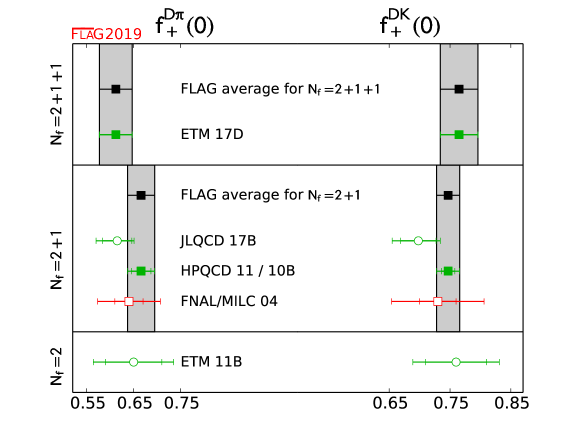
Figure 21: $D\to\pi\ell\nu$ and $D\to K\ell\nu$ semileptonic form factors at $q^{2}=0$. The HPQCD result for $f_{+}^{D\pi}(0)$ is from HPQCD 11, the one for $f_{+}^{DK}(0)$ represents HPQCD 10B (see Tab. 1).

7.3 Form factors for $\Lambda_{c}\to\Lambda\ell\nu$ semileptonic decays

In recent years, Meinel and collaborators have pioneered the computation of form factors for semileptonic heavy-baryon decays (see also Sec. 8.6). In particular, Ref. [Meinel:2016dqj] deals with $\Lambda_{c}\to\Lambda\ell\nu$ transitions. The motivation for this study is twofold: apart from allowing for a new determination of $|V_{cs}|$ in combination with the recent pioneering experimental measurement of the decay rates in Refs. [Ablikim:2015prg, Ablikim:2016vqd], it allows one to test the techniques previously employed for $b$ baryons in the better-controlled (from the point of view of systematics) charm environment.

The amplitudes of the decays $\Lambda_{c}\to\Lambda\ell\nu$ receive contributions from both the vector and the axial components of the current in the matrix element $\langle\Lambda|\bar{s}\gamma^{\mu}(\mathbf{1}-\gamma_{5})c|\Lambda_{c}\rangle$, and can be parameterized in terms of six different form factors — see, e.g., Ref. [Feldmann:2011xf] for a complete description. They split into three form factors $f_{+}$, $f_{0}$, $f_{\perp}$ in the parity-even sector, mediated by the vector component of the current, and another three form factors $g_{+},g_{0},g_{\perp}$ in the parity-odd sector, mediated by the axial component. All of them provide contributions that are parametrically comparable.

The computation in Meinel 16 [Meinel:2016dqj] uses RBC/UKQCD $N_{f}=2+1$ DWF ensembles, and treats the $c$ quarks within the Columbia RHQ approach. Two values of the lattice spacing ($a\sim 0.11,~{}0.085~{}{\rm fm}$) are considered, with the absolute scale set from the $\Upsilon(2S)$–$\Upsilon(1S)$ splitting. In one ensemble the pion mass $m_{\pi}=139~{}{\rm MeV}$ is at the physical point, while for other ensembles they range roughly in the 300–350 MeV interval. Results for the form factors are obtained from suitable three-point functions, and fitted to a modified $z$-expansion ansatz that combines the $q^{2}$-dependence with the chiral and continuum extrapolations. The paper goes on to quote the predictions for the total rates in the $e$ and $\mu$ channels (where errors are statistical and systematic, respectively)

$$\begin{split}\hbox{$\Gamma(\Lambda_{c}\to\Lambda e^{+}\nu_{e})\over|V_{cs}|^{2}$}&=0.2007(71)(74)~{}{\rm ps}^{-1}\,,\\ \hbox{$\Gamma(\Lambda_{c}\to\Lambda\mu^{+}\nu_{\mu})\over|V_{cs}|^{2}$}&=0.1945(69)(72)~{}{\rm ps}^{-1}\,.\end{split}$$ (177)

The combination with the recent experimental determination of the total branching fractions by BESIII in Refs. [Ablikim:2015prg, Ablikim:2016vqd] to extract $|V_{cs}|$ is discussed in Sec. 7.4 below.

7.4 Determinations of $|V_{cd}|$ and $|V_{cs}|$ and test of second-row CKM unitarity

We now interpret the lattice-QCD results for the $D_{(s)}$ meson decays as determinations of the CKM matrix elements $|V_{cd}|$ and $|V_{cs}|$ in the Standard Model.

For the leptonic decays, we use the latest experimental averages from Rosner, Stone and Van de Water for the Particle Data Group [Tanabashi:2018oca]

$$f_{D}|V_{cd}|=45.91(1.05)~{}{\rm MeV}\,,\qquad f_{D_{s}}|V_{cs}|=250.9(4.0)~{}{\rm MeV}\,.$$ (178)

By combining these with the average values of $f_{D}$ and $f_{D_{s}}$ from the individual $N_{f}=2$, $N_{f}=2+1$ and $N_{f}=2+1+1$ lattice-QCD calculations that satisfy the FLAG criteria, we obtain the results for the CKM matrix elements $|V_{cd}|$ and $|V_{cs}|$ in Tab. 32. For our preferred values we use the averaged $N_{f}=2$ and $N_{f}=2+1$ results for $f_{D}$ and $f_{D_{s}}$ in Eqs. (162-170). We obtain

$${\rm leptonic~{}decays},N_{f}=2+1+1: |V_{cd}| =0.2166(7)(50)\,, |V_{cs}| =1.004(2)(16)\,,$$ (179)

$${\rm leptonic~{}decays},N_{f}=2+1: |V_{cd}| =0.2197(25)(50)\,, |V_{cs}| =1.012(7)(16)\,,$$ (180)

$${\rm leptonic~{}decays},N_{f}=2: |V_{cd}| =0.2207(74)(50)\,, |V_{cs}| =1.035(25)(16)\,,$$ (181)

where the errors shown are from the lattice calculation and experiment (plus nonlattice theory), respectively. For the $N_{f}=2+1$ and the $N_{f}=2+1+1$ determinations, the uncertainties from the lattice-QCD calculations of the decay constants are smaller than the experimental uncertainties in the branching fractions. Although the results for $|V_{cs}|$ are slightly larger than one, they are consistent with unity within at most 1.5 standard deviations.

The leptonic determinations of these CKM matrix elements have uncertainties that are reaching the few-percent level. However, higher-order electroweak and hadronic-structure dependent corrections to the rate have not been computed for the case of $D_{(s)}$ mesons, whereas they have been estimated to be around 1–2% for pion and kaon decays [Cirigliano:2007ga]. It is therefore important that such theoretical calculations are tackled soon, perhaps directly on the lattice, as proposed in Ref. [Carrasco:2015xwa].

Collaboration	Ref.	$N_{f}$	from	$|V_{cd}|$ or $|V_{cs}|$
FNAL/MILC 17	[Bazavov:2017lyh]	2+1+1	$f_{D}$	0.2165(6)(50)
ETM 17D/Riggio 17	[Lubicz:2017syv, Riggio:2017zwh]	2+1+1	$D\to\pi\ell\nu$	0.2341(74)
ETM 14E	[Carrasco:2014poa]	2+1+1	$f_{D}$	0.2214(41)(51)
RBC/UKQCD 17	[Boyle:2017jwu]	2+1	$f_{D}$	0.2200(36)(50)
HPQCD 12A	[Na:2012iu]	2+1	$f_{D}$	0.2204(36)(50)
HPQCD 11	[Na:2011mc]	2+1	$D\to\pi\ell\nu$	0.2140(93)(29)
FNAL/MILC 11	[Bazavov:2011aa]	2+1	$f_{D}$	0.2097(108)(48)
ETM 13B	[Carrasco:2013zta]	2	$f_{D}$	0.2207(74)(50)
FNAL/MILC 17	[Bazavov:2017lyh]	2+1+1	$f_{D_{s}}$	1.004(2)(16)
ETM 17D/Riggio 17	[Lubicz:2017syv, Riggio:2017zwh]	2+1+1	$D\to K\ell\nu$	0.970(33)
ETM 14E	[Carrasco:2014poa]	2+1+1	$f_{D_{s}}$	1.015(17)(16)
RBC/UKQCD 17	[Boyle:2017jwu]	2+1	$f_{D_{s}}$	1.018(9)(16)
Meinel 16	[Meinel:2016dqj]	2+1	$\Lambda_{c}\to\Lambda\ell\nu$	0.949(24)(51)
$\chi$QCD 14	[Yang:2014sea]	2+1	$f_{D_{s}}$	0.988(17)(16)
FNAL/MILC 11	[Bazavov:2011aa]	2+1	$f_{D_{s}}$	0.965(40)(16)
HPQCD 10A	[Davies:2010ip]	2+1	$f_{D_{s}}$	1.012(10)(16)
HPQCD 10B	[Na:2010uf]	2+1	$D\to K\ell\nu$	0.975(25)(7)
Blossier 18	[Blossier:2018jol]	2	$f_{D_{s}}$	1.054(24)(17)
ETM 13B	[Carrasco:2013zta]	2	$f_{D_{s}}$	1.004(28)(16)

Table 32: Determinations of $|V_{cd}|$ (upper panel) and $|V_{cs}|$ (lower panel) obtained from lattice calculations of $D$-meson leptonic decay constants and semileptonic form factors. The errors shown are from the lattice calculation and experiment (plus nonlattice theory), respectively, save for ETM 17D/Riggio 17, where the joint fit to lattice and experimental data does not provide a separation of the two sources of error (although the latter is still largely theory-dominated).

For $D$ meson semileptonic decays, there is no update on the lattice side from the previous version of our review for $N_{f}=2+1$, where the only works entering the FLAG averages are HPQCD 10B/11 [Na:2010uf, Na:2011mc], that provide values for $f_{+}^{DK}(0)$ and $f_{+}^{D\pi}(0)$, respectively, cf. Eq. (175). The latter can be combined with the latest experimental averages from the HFLAV collaboration [Amhis:2016xyh]:

$$f_{+}^{D\pi}(0)|V_{cd}|=0.1426(19)\,,\qquad f_{+}^{DK}(0)|V_{cs}|=0.7226(34)\,,$$ (182)

where we have combined the experimental statistical and systematic errors in quadrature, to determine the CKM parameters.

The new $N_{f}=2+1+1$ result for form factors in ETM 17D [Lubicz:2017syv] has a broader scope, in that a companion paper [Riggio:2017zwh] provides a determination of $|V_{cd}|$ and $|V_{cs}|$ from a joint fit to lattice and experimental data. This procedure is a priori preferable to the matching at $q^{2}=0$, and we will therefore use the values in Ref. [Riggio:2017zwh] for our CKM averages. It has to be stressed that this entails a measure of bias in the comparison with the above $N_{f}=2+1$ result; to quantify the effect, we also show in Fig. 22 the values of $|V_{cd}|$ and $|V_{cs}|$ obtained by using the values for $f_{+}(0)$ quoted in [Lubicz:2017syv], cf. Eq. (176), together with Eq. (182).

Finally, Meinel 16 has determined the form factors for $\Lambda_{c}\to\Lambda\ell\nu$ decays for $N_{f}=2+1$, which results in a determination of $|V_{cs}|$ in combination with the experimental measurement of the branching fractions for the $e^{+}$ and $\mu^{+}$ channels in Refs. [Ablikim:2015prg, Ablikim:2016vqd]. In Ref. [Meinel:2016dqj] the value $|V_{cs}|=0.949(24)(14)(49)$ is quoted, where the first error comes from the lattice computation, the second from the $\Lambda_{c}$ lifetime, and the third from the branching fraction of the decay. While the lattice uncertainty is competitive with meson channels, the experimental uncertainty is far larger.

We thus proceed to quote our estimates from semileptonic decay as

$$|V_{cd}| =0.2141(93)(29) \ref{~}\mbox{\cite[cite]{[\@@bibref{Number}{Na:2011mc}{}{}]}},$$

$$\mbox{SL~{}averages~{}for}~{}N_{f}=2+1:$$ (183)

$$|V_{cs}|(D) =0.967(25)(5) \ref{~}\mbox{\cite[cite]{[\@@bibref{Number}{Na:2010uf}{}{}]}},$$

$$|V_{cs}|(\Lambda_{c}) =0.949(24)(51) \ref{~}\mbox{\cite[cite]{[\@@bibref{Number}{Meinel:2016dqj}{}{}]}},$$

$$|V_{cd}| =0.2341(74) \,\mathrm{Refs.}~{}\mbox{\cite[cite]{[\@@bibref{Number}{Lubicz:2017syv,Riggio:2017zwh}{}{}]}},$$

$$\mbox{SL~{}averages~{}for}~{}N_{f}=2+1+1:$$ (184)

$$|V_{cs}| =0.970(33) \,\mathrm{Refs.}~{}\mbox{\cite[cite]{[\@@bibref{Number}{Lubicz:2017syv,Riggio:2017zwh}{}{}]}},$$

where the errors for $N_{f}=2+1$ are lattice and experimental (plus nonlattice theory), respectively. It has to be stressed that all errors are largely theory-dominated. The above values are compared with individual leptonic determinations in Tab. 32.

In Tab. 33 we summarize the results for $|V_{cd}|$ and $|V_{cs}|$ from leptonic and semileptonic decays, and compare them to determinations from neutrino scattering (for $|V_{cd}|$ only) and CKM unitarity. These results are also plotted in Fig. 22. For both $|V_{cd}|$ and $|V_{cs}|$, the errors in the direct determinations from leptonic and semileptonic decays are approximately one order of magnitude larger than the indirect determination from CKM unitarity. The direct and indirect determinations are still always compatible within at most $1.2\sigma$, save for the leptonic determinations of $|V_{cs}|$—that show a $\sim 2\sigma$ deviation for all values of $N_{f}$—and $|V_{cd}|$ using the $N_{f}=2+1+1$ lattice result, where the difference is $1.8\sigma$.

In order to provide final estimates, we average all the available results separately for each value of $N_{f}$. In all cases, we assume that results that share a significant fraction of the underlying gauge ensembles have statistical errors that are 100% correlated; the same applies to the heavy-quark discretization and scale setting errors in HPQCD calculations of leptonic and semileptonic decays. Finally, we include a 100% correlation in the fraction of the error of $|V_{cd(s)}|$ leptonic determinations that comes from the experimental input, to avoid an artificial reduction of the experimental uncertainty in the averages. We finally quote

$${\rm our~{}average},N_{f}=2+1+1: |V_{cd}| =0.2219(43)\,, |V_{cs}| =1.002(14)\,,$$ (185)

$${\rm our~{}average},N_{f}=2+1: |V_{cd}| =0.2182(50)\,, |V_{cs}| =0.999(14)\,,$$ (186)

$${\rm our~{}average},N_{f}=2: |V_{cd}| =0.2207(89)\,, |V_{cs}| =1.031(30)\,,$$ (187)

where the errors include both theoretical and experimental uncertainties. These averages also appear in Fig. 22. The mutual consistency between the various lattice results is always good, save for the case of $|V_{cd}|$ with $N_{f}=2+1+1$, where a $\sim 2\sigma$ tension between the leptonic and semileptonic determinations shows up. Currently, the leptonic and semileptonic determinations of $V_{cd}$ are controlled by experimental and lattice uncertainties, respectively. The leptonic error will be reduced by Belle II and BES III. It would be valuable to have other lattice calculations of the semileptonic form factors.

Using the lattice determinations of $|V_{cd}|$ and $|V_{cs}|$ in Tab. 33, we can test the unitarity of the second row of the CKM matrix. We obtain

$$N_{f}=2+1+1: |V_{cd}|^{2}+|V_{cs}|^{2}+|V_{cb}|^{2}-1 =0.05(3)\,,$$ (188)

$$N_{f}=2+1: |V_{cd}|^{2}+|V_{cs}|^{2}+|V_{cb}|^{2}-1 =0.05(3)\,,$$ (189)

$$N_{f}=2: |V_{cd}|^{2}+|V_{cs}|^{2}+|V_{cb}|^{2}-1 =0.11(6)\,.$$ (190)

Again, tensions at the 2$\sigma$ level with CKM unitarity are visible, as also reported in the PDG review [Rosner:2015wva], where the value 0.063(34) is quoted for the quantity in the equations above. Given the current level of precision, this result does not depend on $|V_{cb}|$, which is of $\mathcal{O}(10^{-2})$.

	from	Ref.	$|V_{cd}|$	$|V_{cs}|$
$N_{f}=2+1+1$	$f_{D}$ & $f_{D_{s}}$		0.2166(50)	1.004(16)
$N_{f}=2+1$	$f_{D}$ & $f_{D_{s}}$		0.2197(56)	1.012(17)
$N_{f}=2$	$f_{D}$ & $f_{D_{s}}$		0.2207(89)	1.035(30)
$N_{f}=2+1+1$	$D\to\pi\ell\nu$ and $D\to K\ell\nu$		0.2341(74)	0.970(33)
$N_{f}=2+1$	$D\to\pi\ell\nu$ and $D\to K\ell\nu$		0.2141(97)	0.967(25)
$N_{f}=2+1$	$\Lambda_{c}\to\Lambda\ell\nu$		n/a	0.949(56)
PDG	neutrino scattering	[Tanabashi:2018oca]	0.230(11)
Rosner 15 (for the PDG)	CKM unitarity	[Rosner:2015wva]	0.2254(7)	0.9733(2)

Table 33: Comparison of determinations of $|V_{cd}|$ and $|V_{cs}|$ obtained from lattice methods with nonlattice determinations and the Standard Model prediction assuming CKM unitarity.

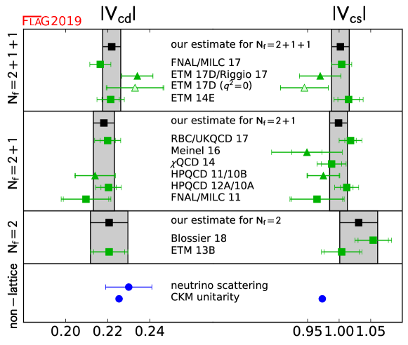
Figure 22: Comparison of determinations of $|V_{cd}|$ and $|V_{cs}|$ obtained from lattice methods with nonlattice determinations and the Standard Model prediction based on CKM unitarity. When two references are listed on a single row, the first corresponds to the lattice input for $|V_{cd}|$ and the second to that for $|V_{cs}|$. The results denoted by squares are from leptonic decays, while those denoted by triangles are from semileptonic decays. The points indicated as ETM 17D ($q^{2}=0$) do not contribute to the average, and are shown for comparison purposes (see text).

8 $B$-meson decay constants, mixing parameters and form factors

Authors: Y. Aoki, D. Bečirević, M. Della Morte, S. Gottlieb, D. Lin, E. Lunghi, C. Pena

The (semi)leptonic decay and mixing processes of $B_{(s)}$ mesons have been playing a crucial role in flavour physics. In particular, they contain important information for the investigation of the $b{-}d$ unitarity triangle in the Cabibbo-Kobayashi-Maskawa (CKM) matrix, and can be ideal probes of physics beyond the Standard Model. The charged-current decay channels $B^{+}\rightarrow l^{+}\nu_{l}$ and $B^{0}\rightarrow\pi^{-}l^{+}\nu_{l}$, where $l^{+}$ is a charged lepton with $\nu_{l}$ being the corresponding neutrino, are essential in extracting the CKM matrix element $|V_{ub}|$. Similarly, the $B$ to $D^{(\ast)}$ semileptonic transitions can be used to determine $|V_{cb}|$. The flavour-changing neutral current (FCNC) processes, such as $B\to K^{(*)}\ell^{+}\ell^{-}$ and $B_{d(s)}\to\ell^{+}\ell^{-}$, occur only beyond the tree level in weak interactions and are suppressed in the Standard Model. Therefore, these processes can be sensitive to new physics, since heavy particles can contribute to the loop diagrams. They are also suitable channels for the extraction of the CKM matrix elements involving the top quark which can appear in the loop. The decays $B\to D^{(*)}\ell\nu$ and $B\to K^{(*)}\ell\ell$ can also be used to test lepton flavour universality by comparing results for $\ell=e$, $\mu$ and $\tau$. In particular, anomalies have been seen in the ratios $R(D^{(*)})={\cal B}(B\to D^{(*)}\tau\nu)/{\cal B}(B\to D^{(*)}\ell\nu)_{\ell=e,\mu}$ and ${R}(K^{(*)})={\cal B}(B\to K^{(*)}\mu\mu)/{\cal B}(B\to K^{(*)}ee)$. In addition, the neutral $B_{d(s)}$-meson mixings are FCNC processes and are dominated by the 1-loop “box” diagrams containing the top quark and the $W$ bosons. Thus, using the experimentally measured neutral $B^{0}_{d(s)}$-meson oscillation frequencies, $\Delta M_{d(s)}$, and the theoretical calculations for the relevant hadronic mixing matrix elements, one can obtain $|V_{td}|$ and $|V_{ts}|$ in the Standard Model.

Accommodating the light quarks and the $b$ quark simultaneously in lattice-QCD computations is a challenging endeavour. To incorporate the pion and the $b$ hadrons with their physical masses, the simulations have to be performed using the lattice size $\hat{L}=L/a\sim\mathcal{O}(10^{2})$, where $a$ is the lattice spacing and $L$ is the physical (dimensionful) box size. The most ambitious calculations are now using such volumes; however, many ensembles are smaller. Therefore, in addition to employing Chiral Perturbation Theory for the extrapolations in the light-quark mass, current lattice calculations for quantities involving $b$ hadrons often make use of effective theories that allow one to expand in inverse powers of $m_{b}$. In this regard, two general approaches are widely adopted. On the one hand, effective field theories such as Heavy-Quark Effective Theory (HQET) and Nonrelativistic QCD (NRQCD) can be directly implemented in numerical computations. On the other hand, a relativistic quark action can be improved à la Symanzik to suppress cutoff errors, and then re-interpreted in a manner that is suitable for heavy-quark physics calculations. This latter strategy is often referred to as the method of the Relativistic Heavy-Quark Action (RHQA). The utilization of such effective theories inevitably introduces systematic uncertainties that are not present in light-quark calculations. These uncertainties can arise from the truncation of the expansion in constructing the effective theories (as in HQET and NRQCD), or from more intricate cutoff effects (as in NRQCD and RQHA). They can also be introduced through more complicated renormalization procedures which often lead to significant systematic effects in matching the lattice operators to their continuum counterparts. For instance, due to the use of different actions for the heavy and the light quarks, it is more difficult to construct absolutely normalized bottom-light currents.

Complementary to the above “effective theory approaches”, another popular method is to simulate the heavy and the light quarks using the same (normally improved) lattice action at several values of the heavy-quark mass $m_{h}$ with $am_{h}<1$ and $m_{h}<m_{b}$. This enables one to employ HQET-inspired relations to extrapolate the computed quantities to the physical $b$ mass. When combined with results obtained in the static heavy-quark limit, this approach can be rendered into an interpolation, instead of extrapolation, in $m_{h}$. The discretization errors are the main source of the systematic effects in this method, and very small lattice spacings are needed to keep such errors under control.

In recent years, it has also been possible to perform lattice simulations at very fine lattice spacings and treat heavy quarks as fully relativistic fermions without resorting to effective field theories. Such simulations are of course very demanding in computing resources.

Because of the challenge described above, the efforts that have been made to obtain reliable, accurate lattice-QCD results for physics of the $b$ quark have been enormous. These efforts include significant theoretical progress in formulating QCD with heavy quarks on the lattice. This aspect is briefly reviewed in Appendix LABEL:app:HQactions.

In this section, we summarize the results of the $B$-meson leptonic decay constants, the neutral $B$-mixing parameters, and the semileptonic form factors, from lattice QCD. To be focused on the calculations that have strong phenomenological impact, we limit the review to results based on modern simulations containing dynamical fermions with reasonably light pion masses (below approximately 500 MeV). There has been significant progress for $b$-quark physics since the previous review. There are also a number of calculations that are still in a preliminary stage. We have made note of some of these in anticipation of later publications, whose results will contribute to future averages.

Following our review of $B_{(s)}$-meson leptonic decay constants, the neutral $B$-meson mixing parameters, and semileptonic form factors, we then interpret our results within the context of the Standard Model. We combine our best-determined values of the hadronic matrix elements with the most recent experimentally-measured branching fractions to obtain $|V_{ub}|$ and $|V_{cb}|$, and compare these results to those obtained from inclusive semileptonic $B$ decays.

Recent lattice-QCD averages for $B^{+}$- and $B_{s}$-meson decay constants were also presented by the Particle Data Group (PDG) in Ref. [Rosner:2015wva]. The PDG three- and four-flavour averages for these quantities differ from those quoted here because the PDG provides the charged-meson decay constant $f_{B^{+}}$, while we present the isospin-averaged meson-decay constant $f_{B}$.

8.1 Leptonic decay constants $f_{B}$ and $f_{B_{s}}$

The $B$- and $B_{s}$-meson decay constants are crucial inputs for extracting information from leptonic $B$ decays. Charged $B$ mesons can decay to the lepton-neutrino final state through the charged-current weak interaction. On the other hand, neutral $B_{d(s)}$ mesons can decay to a charged-lepton pair via a flavour-changing neutral current (FCNC) process.

In the Standard Model the decay rate for $B^{+}\to\ell^{+}\nu_{\ell}$ is described by a formula identical to Eq. (160), with $D_{(s)}$ replaced by $B$, and the relevant CKM matrix element $V_{cq}$ replaced by $V_{ub}$,

$$\Gamma(B\to\ell\nu_{\ell})=\hbox{$m_{B}\over 8\pi$}G_{F}^{2}f_{B}^{2}|V_{ub}|^{2}m_{\ell}^{2}\left(1-\hbox{$m_{\ell}^{2}\over m_{B}^{2}$}\right)^{2}\;.$$ (191)

The only charged-current $B$-meson decay that has been observed so far is $B^{+}\to\tau^{+}\nu_{\tau}$, which has been measured by the Belle and Babar collaborations [Lees:2012ju, Kronenbitter:2015kls]. Both collaborations have reported results with errors around $20\%$. These measurements can be used to determine $|V_{ub}|$ when combined with lattice-QCD predictions of the corresponding decay constant.

Neutral $B_{d(s)}$-meson decays to a charged-lepton pair $B_{d(s)}\rightarrow l^{+}l^{-}$ is a FCNC process, and can only occur at one loop in the Standard Model. Hence these processes are expected to be rare, and are sensitive to physics beyond the Standard Model. The corresponding expression for the branching fraction has the form

$$B(B_{q}\to\ell^{+}\ell^{-})=\tau_{B_{q}}\hbox{$G_{F}^{2}\over\pi$}\,Y\,\left(\hbox{$\alpha\over 4\pi\sin^{2}\Theta_{W}$}\right)^{2}m_{B_{q}}f_{B_{q}}^{2}|V_{tb}^{*}V_{tq}|^{2}m_{\ell}^{2}\sqrt{1-4\hbox{$m_{\ell}^{2}\over m_{B}^{2}$}}\;,$$ (192)

where the light quark $q=s$ or $d$, and the function $Y$ includes NLO QCD and electro-weak corrections [Inami:1980fz, Buchalla:1993bv]. Evidence for both $B_{s}\to\mu^{+}\mu^{-}$ and $B_{s}\to\mu^{+}\mu^{-}$ decays was first observed by the CMS and the LHCb collaborations, and a combined analysis was presented in 2014 in Ref. [CMS:2014xfa]. In 2017, the LHCb collaboration reported their latest measurements as [Aaij:2017vad]

$$B(B_{d}\to\mu^{+}\mu^{-}) = (1.5^{+1.2+0.2}_{-1.0-0.1})\,10^{-10},$$

$$B(B_{s}\to\mu^{+}\mu^{-}) = (3.0\pm 0.6^{+0.3}_{-0.2})\,10^{-9},$$ (193)

which are compatible with the Standard Model predictions [Bobeth:2013uxa].

The decay constants $f_{B_{q}}$ (with $q=u,d,s$) parameterize the matrix elements of the corresponding axial-vector currents $A^{\mu}_{bq}=\bar{b}\gamma^{\mu}\gamma^{5}q$ analogously to the definition of $f_{D_{q}}$ in Sec. 7.1:

$$\langle 0|A^{\mu}|B_{q}(p)\rangle=ip_{B}^{\mu}f_{B_{q}}\;.$$ (194)

For heavy-light mesons, it is convenient to define and analyse the quantity

$$\Phi_{B_{q}}\equiv f_{B_{q}}\sqrt{m_{B_{q}}}\;,$$ (195)

which approaches a constant (up to logarithmic corrections) in the $m_{B}\to\infty$ limit because of the heavy-quark symmetry. In the following discussion we denote lattice data for $\Phi$($f$) obtained at a heavy-quark mass $m_{h}$ and light valence-quark mass $m_{\ell}$ as $\Phi_{h\ell}$($f_{hl}$), to differentiate them from the corresponding quantities at the physical $b$- and light-quark masses.

The $SU(3)$-breaking ratio $f_{B_{s}}/f_{B}$ is of phenomenological interest. This is because in lattice-QCD calculations for this quantity, many systematic effects can be partially reduced. These include discretization errors, heavy-quark mass tuning effects, and renormalization/ matching errors, amongst others. On the other hand, this $SU(3)$-breaking ratio is still sensitive to the chiral extrapolation. Given that the chiral extrapolation is under control, one can then adopt $f_{B_{s}}/f_{B}$ as input in extracting phenomenologically-interesting quantities. In addition, it often happens to be easier to obtain lattice results for $f_{B_{s}}$ with smaller errors. Therefore, one can combine the $B_{s}$-meson decay constant with the $SU(3)$-breaking ratio to calculate $f_{B}$. Such a strategy can lead to better precision in the computation of the $B$-meson decay constant, and has been adopted by the ETM [Carrasco:2013zta, Bussone:2016iua] and the HPQCD collaborations [Na:2012sp].

It is clear that the decay constants for charged and neutral $B$ mesons play different roles in flavour-physics phenomenology. As already mentioned above, the knowledge of the $B^{+}$-meson decay constant $f_{B^{+}}$ is essential for extracting $|V_{ub}|$ from leptonic $B^{+}$ decays. The neutral $B$-meson decay constants $f_{B^{0}}$ and $f_{B_{s}}$ are inputs for the search of new physics in rare leptonic $B^{0}$ decays. In view of this, it is desirable to include isospin-breaking effects in lattice computations for these quantities, and have results for $f_{B^{+}}$ and $f_{B^{0}}$. With the increasing precision of recent lattice calculations, isospin splittings for $B$-meson decay constants are significant, and will play an important role in the foreseeable future. A few collaborations reported $f_{B^{+}}$ and $f_{B^{0}}$ separately by taking into account strong isospin effects in the valence sector, and estimated the corrections from electromagnetism. To properly use these results for extracting phenomenologically relevant information, one would have to take into account QED effects in the $B$-meson leptonic decay rates. Currently, errors on the experimental measurements on these decay rates are still very large. In this review, we will then concentrate on the isospin-averaged result $f_{B}$ and the $B_{s}$-meson decay constant, as well as the $SU(3)$-breaking ratio $f_{B_{s}}/f_{B}$. For the world average for lattice determination of $f_{B^{+}}$ and $f_{B_{s}}/f_{B^{+}}$, we refer the reader to the latest work from the Particle Data Group (PDG) [Rosner:2015wva]. Notice that the $N_{f}=2+1$ lattice results used in Ref. [Rosner:2015wva] and the current review are identical. We will discuss this in further detail at the end of this subsection.

The status of lattice-QCD computations for $B$-meson decay constants and the $SU(3)$-breaking ratio, using gauge-field ensembles with light dynamical fermions, is summarized in Tabs. 1 and 1, while Figs. 23 and 24 contain the graphical presentation of the collected results and our averages. Many results in these tables and plots were already reviewed in detail in the previous FLAG report. Below we will describe the new results that appeared after January 2016.

Collaboration

Ref.

$N_{f}$

publication status

continuum extrapolation

chiral extrapolation

finite volume

renormalization/matching

heavy-quark treatment

$f_{B^{+}}$

$f_{B^{0}}$

$f_{B}$

$f_{B_{s}}$

FNAL/MILC 17

[Bazavov:2017lyh]

2+1+1

A

$\bigstar$

$\bigstar$

$\bigstar$

$\bigstar$

✓

189.4(1.4)

190.5(1.3)

189.9(1.4)

230.7(1.2)

HPQCD 17A

[Hughes:2017spc]

2+1+1

A

$\bigstar$

$\bigstar$

$\bigstar$

$\circ$

✓

$-$

$-$

196(6)

236(7)

ETM 16B

[Bussone:2016iua]

2+1+1

A

$\bigstar$

$\circ$

$\circ$

$\circ$

✓

$-$

$-$

193(6)

229(5)

ETM 13E

[Carrasco:2013naa]

2+1+1

C

$\bigstar$

$\circ$

$\circ$

$\circ$

✓

$-$

$-$

196(9)

235(9)

HPQCD 13

[Dowdall:2013tga]

2+1+1

A

$\bigstar$

$\bigstar$

$\bigstar$

$\circ$

✓

184(4)

188(4)

186(4)

224(5)

RBC/UKQCD 14

[Christ:2014uea]

2+1

A

$\circ$

$\circ$

$\circ$

$\circ$

✓

195.6(14.9)

199.5(12.6)

$-$

235.4(12.2)

RBC/UKQCD 14A

[Aoki:2014nga]

2+1

A

$\circ$

$\circ$

$\circ$

$\circ$

✓

$-$

$-$

219(31)

264(37)

RBC/UKQCD 13A

[Witzel:2013sla]

2+1

C

$\circ$

$\circ$

$\circ$

$\circ$

✓

$-$

$-$

191(6)${}_{\rm stat}^{\diamond}$

233(5)${}_{\rm stat}^{\diamond}$

HPQCD 12

[Na:2012sp]

2+1

A

$\circ$

$\circ$

$\circ$

$\circ$

✓

$-$

$-$

191(9)

228(10)

HPQCD 12

[Na:2012sp]

2+1

A

$\circ$

$\circ$

$\circ$

$\circ$

✓

$-$

$-$

189(4)${}^{\triangle}$

$-$

HPQCD 11A

[McNeile:2011ng]

2+1

A

$\bigstar$

$\circ$

$\bigstar$

$\bigstar$

✓

$-$

$-$

$-$

225(4)${}^{\nabla}$

FNAL/MILC 11

[Bazavov:2011aa]

2+1

A

$\circ$

$\circ$

$\bigstar$

$\circ$

✓

197(9)

$-$

$-$

242(10)

HPQCD 09

[Gamiz:2009ku]

2+1

A

$\circ$

$\circ$

$\circ$

$\circ$

✓

$-$

$-$

190(13)${}^{\bullet}$

231(15)${}^{\bullet}$

ALPHA 14

[Bernardoni:2014fva]

2

A

$\bigstar$

$\bigstar$

$\bigstar$

$\bigstar$

✓

$-$

$-$

186(13)

224(14)

ALPHA 13

[Bernardoni:2013oda]

2

C

$\bigstar$

$\bigstar$

$\bigstar$

$\bigstar$

✓

$-$

$-$

187(12)(2)

224(13)

ETM 13B, 13C${}^{\dagger}$

[Carrasco:2013zta, Carrasco:2013iba]

2

A

$\bigstar$

$\circ$

$\bigstar$

$\circ$

✓

$-$

$-$

189(8)

228(8)

ALPHA 12A

[Bernardoni:2012ti]

2

C

$\bigstar$

$\bigstar$

$\bigstar$

$\bigstar$

✓

$-$

$-$

193(9)(4)

219(12)

ETM 12B

[Carrasco:2012de]

2

C

$\bigstar$

$\circ$

$\bigstar$

$\circ$

✓

$-$

$-$

197(10)

234(6)

ALPHA 11

[Blossier:2011dk]

2

C

$\bigstar$

$\circ$

$\bigstar$

$\bigstar$

✓

$-$

$-$

174(11)(2)

$-$

ETM 11A

[Dimopoulos:2011gx]

2

A

$\circ$

$\circ$

$\bigstar$

$\circ$

✓

$-$

$-$

195(12)

232(10)

ETM 09D

[Blossier:2009hg]

2

A

$\circ$

$\circ$

$\circ$

$\circ$

✓

$-$

$-$

194(16)

235(12)

${}^{\diamond}$Statistical errors only.

${}^{\triangle}$Obtained by combining $f_{B_{s}}$ from HPQCD 11A with $f_{B_{s}}/f_{B}$ calculated in this work.

${}^{\nabla}$This result uses one ensemble per lattice spacing with light to strange sea-quark mass ratio $m_{\ell}/m_{s}\approx 0.2$.

${}^{\bullet}$This result uses an old determination of $r_{1}=0.321(5)$ fm from Ref. [Gray:2005ur] that has since been superseded.

${}^{\dagger}$Update of ETM 11A and 12B.

Table 34: Decay constants of the $B$, $B^{+}$, $B^{0}$ and $B_{s}$ mesons (in MeV). Here $f_{B}$ stands for the mean value of $f_{B^{+}}$ and $f_{B^{0}}$, extrapolated (or interpolated) in the mass of the light valence-quark to the physical value of $m_{ud}$.

Collaboration

Ref.

$N_{f}$

publication status

continuum extrapolation

chiral extrapolation

finite volume

renormalization/matching

heavy-quark treatment

$f_{B_{s}}/f_{B^{+}}$

$f_{B_{s}}/f_{B^{0}}$

$f_{B_{s}}/f_{B}$

FNAL/MILC 17

[Bazavov:2017lyh]

2+1+1

A

$\bigstar$

$\bigstar$

$\bigstar$

$\bigstar$

✓

1.2180(49)

1.2109(41)

$-$

HPQCD 17A

[Hughes:2017spc]

2+1+1

A

$\bigstar$

$\bigstar$

$\bigstar$

$\circ$

✓

$-$

$-$

1.207(7)

ETM 16B

[Bussone:2016iua]

2+1+1

A

$\bigstar$

$\circ$

$\circ$

$\circ$

✓

$-$

$-$

1.184(25)

ETM 13E

[Carrasco:2013naa]

2+1+1

C

$\bigstar$

$\circ$

$\circ$

$\circ$

✓

$-$

$-$

1.201(25)

HPQCD 13

[Dowdall:2013tga]

2+1+1

A

$\bigstar$

$\bigstar$

$\bigstar$

$\circ$

✓

1.217(8)

1.194(7)

1.205(7)

RBC/UKQCD 14

[Christ:2014uea]

2+1

A

$\circ$

$\circ$

$\circ$

$\circ$

✓

1.223(71)

1.197(50)

$-$

RBC/UKQCD 14A

[Aoki:2014nga]

2+1

A

$\circ$

$\circ$

$\circ$

$\circ$

✓

$-$

$-$

1.193(48)

RBC/UKQCD 13A

[Witzel:2013sla]

2+1

C

$\circ$

$\circ$

$\circ$

$\circ$

✓

$-$

$-$

1.20(2)${}_{\rm stat}^{\diamond}$

HPQCD 12

[Na:2012sp]

2+1

A

$\circ$

$\circ$

$\circ$

$\circ$

✓

$-$

$-$

1.188(18)

FNAL/MILC 11

[Bazavov:2011aa]

2+1

A

$\circ$

$\circ$

$\bigstar$

$\circ$

✓

1.229(26)

$-$

$-$

RBC/UKQCD 10C

[Albertus:2010nm]

2+1

A

$\blacksquare$

$\blacksquare$

$\blacksquare$

$\circ$

✓

$-$

$-$

1.15(12)

HPQCD 09

[Gamiz:2009ku]

2+1

A

$\circ$

$\circ$

$\circ$

$\circ$

✓

$-$

$-$

1.226(26)

ALPHA 14

​​​[Bernardoni:2014fva]

2

A

$\bigstar$

$\bigstar$

$\bigstar$

$\bigstar$

✓

$-$

$-$

1.203(65)

ALPHA 13

[Bernardoni:2013oda]

2

C

$\bigstar$

$\bigstar$

$\bigstar$

$\bigstar$

✓

$-$

$-$

1.195(61)(20)

ETM 13B, 13C${}^{\dagger}$

[Carrasco:2013zta, Carrasco:2013iba]

2

A

$\bigstar$

$\circ$

$\bigstar$

$\circ$

✓

$-$

$-$

1.206(24)

ALPHA 12A

[Bernardoni:2012ti]

2

C

$\bigstar$

$\bigstar$

$\bigstar$

$\bigstar$

✓

$-$

$-$

1.13(6)

ETM 12B

[Carrasco:2012de]

2

C

$\bigstar$

$\circ$

$\bigstar$

$\circ$

✓

$-$

$-$

1.19(5)

ETM 11A

[Dimopoulos:2011gx]

2

A

$\circ$

$\circ$

$\bigstar$

$\circ$

✓

$-$

$-$

1.19(5)

${}^{\diamond}$Statistical errors only.

${}^{\dagger}$Update of ETM 11A and 12B.

Table 35: Ratios of decay constants of the $B$ and $B_{s}$ mesons (for details see Tab. 1).

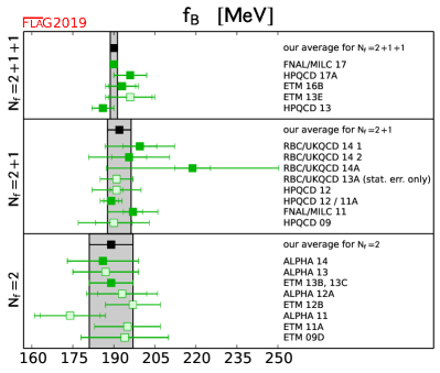
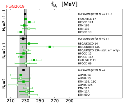
Figure 23: Decay constants of the $B$ and $B_{s}$ mesons. The values are taken from Tab. 1 (the $f_{B}$ entry for FNAL/MILC 11 represents $f_{B^{+}}$). The significance of the colours is explained in Sec. 2. The black squares and grey bands indicate our averages in Eqs. (196), (199), (202), (197), (200) and (203).

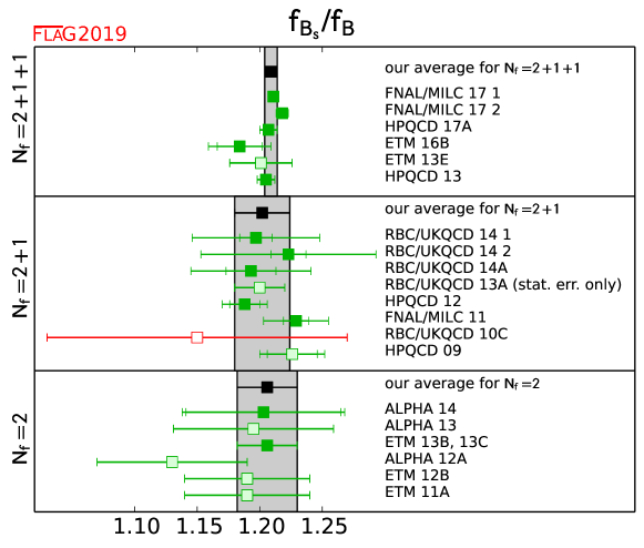
Figure 24: Ratio of the decay constants of the $B$ and $B_{s}$ mesons. The values are taken from Tab. 1. Results labelled as FNAL/MILC 17 1 and FNAL/MILC 17 2 correspond to those for $f_{B_{s}}/f_{B^{0}}$ and $f_{B_{s}}/f_{B^{+}}$ reported in FNAL/MILC 17. The significance of the colours is explained in Sec. 2. The black squares and grey bands indicate our averages in Eqs. (198), (201) and (204).

No new $N_{f}=2$ and $N_{f}=2+1$ project for computing $f_{B}$, $f_{B_{s}}$ and $f_{B_{s}}/f_{B}$ were completed after the publication of the previous FLAG review [Aoki:2016frl]. Therefore, our averages for these cases stay the same as those in Ref. [Aoki:2016frl],

$$N_{f}=2: f_{B} =188(7)\;{\rm MeV} \,\mathrm{Refs.}~{}\mbox{\cite[cite]{[\@@bibref{Number}{Carrasco:2013zta,Bernardoni:2014fva}{}{}]}},$$ (196)

$$N_{f}=2: f_{B_{s}} =227(7)\;{\rm MeV} \,\mathrm{Refs.}~{}\mbox{\cite[cite]{[\@@bibref{Number}{Carrasco:2013zta,Bernardoni:2014fva}{}{}]}},$$ (197)

$$N_{f}=2: f_{B_{s}}\over{f_{B}} =1.206(0.023) \,\mathrm{Refs.}~{}\mbox{\cite[cite]{[\@@bibref{Number}{Carrasco:2013zta,Bernardoni:2014fva}{}{}]}},$$ (198)

$$N_{f}=2+1: f_{B} =192.0(4.3)\;{\rm MeV} \,\mathrm{Refs.}~{}\mbox{\cite[cite]{[\@@bibref{Number}{Bazavov:2011aa,McNeile:2011ng,Na:2012sp,Aoki:2014nga,Christ:2014uea}{}{}]}},$$ (199)

$$N_{f}=2+1: f_{B_{s}} =228.4(3.7)\;{\rm MeV} \,\mathrm{Refs.}~{}\mbox{\cite[cite]{[\@@bibref{Number}{Bazavov:2011aa,McNeile:2011ng,Na:2012sp,Aoki:2014nga,Christ:2014uea}{}{}]}},$$ (200)

$$N_{f}=2+1: f_{B_{s}}\over{f_{B}} =1.201(0.016) \,\mathrm{Refs.}~{}\mbox{\cite[cite]{[\@@bibref{Number}{Bazavov:2011aa,Na:2012sp,Aoki:2014nga,Christ:2014uea}{}{}]}}.$$ (201)

There have been results for $f_{B_{(s)}}$ and $f_{B_{s}}/f_{B}$ from three collaborations, ETMC, HPQCD and FNAL/MILC since the last FLAG report. In Tabs. 1 and 1, these results are labelled ETM 16B [Bussone:2016iua], HPQCD 17A [Hughes:2017spc] and FNAL/MILC 17 [Bazavov:2017lyh].

In ETM 16B [Bussone:2016iua], simulations at three values of lattice spacing, $a=0.0885$, 0.0815 and 0.0619 fm are performed with twisted-mass Wilson fermions and the Iwasaki gauge action. The three lattice spacings correspond to the bare couplings $\beta=1.90$, 1.95 and 2.10. The pion masses in this work range from 210 to 450 MeV, and the lattice sizes are between 1.97 and 2.98 fm. An essential feature in ETM 16B [Bussone:2016iua] is the use of the ratio method [Blossier:2009hg]. In the application of this approach to the $B$-decay constants, one first computes the quantity ${\mathcal{F}}_{hq}\equiv f_{hq}/M_{hq}$, where $f_{hq}$ and $M_{hq}$ are decay constant and mass of the pseudoscalar meson composed of valence (relativistic) heavy quark $h$ and light (or strange) quark $q$. The matching between the lattice and the continuum heavy-light currents for extracting the above $f_{hq}$ is straightforward because the valence heavy quark is also described by twisted-mass fermions. In the second step, the ratio $z_{q}(\bar{\mu}^{(h)},\lambda)\equiv[{\mathcal{F}}_{hq}C_{A}^{{\mathrm{stat}}}(\bar{\mu}^{(h^{\prime})})(\mu_{{\mathrm{pole}}}^{(h)})^{3/2}]/[{\mathcal{F}}_{h^{\prime}q}C_{A}^{{\mathrm{stat}}}(\bar{\mu}^{(h)})(\mu_{{\mathrm{pole}}}^{(h^{\prime})})^{3/2}]$ is calculated, where $\mu_{{\mathrm{pole}}}^{(h)}$ is the pole mass of the heavy quark $h$ with $\bar{\mu}^{(h)}$ being the corresponding renormalized mass in a scheme (chosen to be the $\overline{{\mathrm{MS}}}$ scheme in ETM 16B [Bussone:2016iua]), $C_{A}^{{\mathrm{stat}}}(\bar{\mu}^{(h)})$ is the matching coefficient for the $(hq)$-meson decay constant in QCD and its counterpart in HQET, and $\bar{\mu}^{(h)}=\lambda\bar{\mu}^{(h^{\prime})}$ with $\lambda$ being larger than, but close to, one. The authors of ETM 16B [Bussone:2016iua] use the NNLO perturbative result of $C_{A}^{{\mathrm{stat}}}(\bar{\mu}^{(h)})$ in their work. Notice that in practice one never has to determine the heavy-quark pole mass in this strategy, since it can be matched to the $\overline{{\mathrm{MS}}}$ mass, and the matching coefficient is known to NNNLO [Chetyrkin:1999pq, Chetyrkin:1999ys, Gray:1990yh]. By starting from a “triggering” point with the heavy-quark mass around that of the charm, one can proceed with the calculations in steps, such that $\bar{\mu}^{(h)}$ is increased by a factor of $\lambda$ at each step. In ETM 16B [Bussone:2016iua], the authors went up to heavy-quark mass around 3.3 GeV, and observed that all systematics were under control. In this approach, it is also crucial to employ the information that $z_{q}(\bar{\mu}^{(h)},\lambda)\rightarrow 1$ in the limit $\bar{\mu}^{(h)}\rightarrow\infty$. Designing the computations in such a way that in the last step, $\bar{\mu}^{(h)}$ is equal to the pre-determined bottom-quark mass in the same renormalization scheme, one obtains $f_{B_{(s)}}/M_{B_{(s)}}$. Employing experimental results for $M_{B_{(s)}}$, the decay constants can be extracted. In ETM 16B [Bussone:2016iua], this strategy was implemented to compute $f_{B_{s}}$. It was also performed for a double ratio to determine $(f_{B_{s}}/f_{B})/(f_{K}/f_{\pi})$, hence $f_{B_{s}}/f_{B}$, using information of $f_{K}/f_{\pi}$ from Ref. [Carrasco:2014poa]. This double ratio leads to the advantage that it contains small coefficients for chiral logarithms. The $B$-meson decay constant is then computed with $f_{B}=f_{B_{s}}/(f_{B_{s}}/f_{B})$. The authors estimated various kinds of systematic errors in their work. These include discretization errors, the effects of perturbative matching between QCD and HQET, those of chiral extrapolation, and errors associate with the value of $f_{K}/f_{\pi}$.

The authors of HPQCD 17A [Hughes:2017spc] reanalysed the data in Ref. [Dowdall:2013tga] (HPQCD 13 in Tabs. 1 and 1) employing a different method for computing $B$-decay constants with NRQCD heavy quarks and HISQ light quarks on the lattice. The NRQCD action used in this work is improved to $O(\alpha_{s}v_{b}^{4})$, where $v_{b}$ is the velocity of the $b$ quark. In Ref. [Dowdall:2013tga], the determination of the decay constants is carried out through studying matrix elements of axial currents. On the other hand, the same decay constants can be obtained by investigating $(m_{b}+m_{l})\langle 0|P|B\rangle$, where $m_{b}$ ($m_{l}$) is the $b$- (light-)quark mass and $P$ stands for the pseudoscalar current. The matching of this pseudoscalar current between QCD and NRQCD is performed at the precision of ${\mathcal{O}}(\alpha_{s})$, ${\mathcal{O}}(\alpha_{s}\Lambda_{{\mathrm{QCD}}}/m_{b})$ and ${\mathcal{O}}(\alpha_{s}a\Lambda_{{\mathrm{QCD}}})$, using lattice perturbation theory. This requires the inclusion of three operators in the NRQCD-HISQ theory. The gauge configurations used in this computation were part of those generated by the MILC collaboration, with details given in Ref. [Bazavov:2012xda]. They are the ensembles obtained at three values of bare gauge coupling ($\beta=6.3,6.0$ and 5.8), corresponding to lattice spacings, determined using the $\Upsilon(2S-1A)$ splitting, between 0.09 and 0.15 fm. Pion masses are between 128 and 315 MeV. For each lattice spacing, the MILC collaboration performed simulations at several lattice volumes, such that $M_{\pi}L$ lies between 3.3 and 4.5 for all the data points. This ensures that the finite-size effects are under control [Arndt:2004bg]. On each ensemble, the bare NRQCD quark mass is tuned to the $b$-quark mass using the spin-average for the masses $\Upsilon$ and $\eta_{b}$. In this work, a combined chiral-continuum extrapolation is performed, with the strategy of using Bayesian priors as explained in Ref. [Dowdall:2012ab]. Systematic effects estimated in HPQCD 17A [Hughes:2017spc] include those from lattice-spacing dependence, the chiral fits, the $B{-}B^{\ast}{-}\pi$ axial coupling, the operator matching, and the relativistic corrections to the NRQCD formalism. Although these errors are estimated in the same fashion as in Ref. [Dowdall:2013tga] (HPQCD 13), most of them involve the handling of fits to the actual data. This means that most of the systematics effects from HPQCD 13 [Dowdall:2013tga] and HPQCD 17A [Hughes:2017spc] are not correlated, although the two calculations are performed on exactly the same gauge field ensembles. The only exception is the error in the relativistic corrections. For this, the authors simply take $(\Lambda_{{\mathrm{QCD}}}/m_{b})^{2}\approx 1\%$ as the estimation in both computations. Therefore, we will correlate this part of the systematic effects in our average.

The third new calculation for the $B$-meson decay constants since the last FLAG report was performed by the FNAL/MILC collaboration (FNAL/MILC 17 [Bazavov:2017lyh] in Tabs. 1 and 1). In this work, Ref. [Bazavov:2017lyh], the simulations are performed for six lattice spacings, ranging from 0.03 to 0.15 fm. For the two finest lattices ($a=0.042$ and 0.03 fm), it is found that the topological charge is not well equilibrated. The effects of this nonequilibration are estimated using results of chiral perturbation theory in Ref. [Bernard:2017npd]. Another feature of the simulations is that both RHMC and RHMD algorithms are used. The authors investigated the effects of omitting the Metropolis test in the RHMD simulations by examining changes of the plaquette values, and found that they do not result in any variation with statistical significance. The light-quark masses used in this computation correspond to pion masses between 130 to 314 MeV. The values of the valence heavy-quark mass $m_{h}$ are in the range of about 0.9 and 5 times the charm-quark mass. Notice that on the two coarsest lattices, the authors only implement calculations at $m_{h}\sim m_{c}$ in order to avoid uncontrolled discretization errors, while only on the two finest lattices, is $m_{h}$ chosen to be as high as $\sim 5m_{c}$. For setting the scale and the quark masses, the approach described in Ref. [Bazavov:2014wgs] is employed, with the special feature of using the decay constant of the “fictitious” meson that is composed of degenerate quarks with mass $m_{p4s}=0.4m_{s}$. The overall scale is determined by comparing $f_{\pi}$ to its PDG average as reported in Ref. [Rosner:2015wva]. In the analysis procedure of extrapolating/interpolating to the physical quark masses and the continuum limit, the key point is the use of heavy-meson rooted all-staggered chiral perturbation theory (HMrA$\chi$PT) [Bernard:2013qwa]. In order to account for lattice artifacts and the effects of the heavy-quark mass in this chiral expansion, appropriate polynomial terms in $a$ and $1/m_{h}$ are included in the fit formulae. The full NLO terms in the chiral effective theory are incorporated in the analysis, while only the analytic contributions from the NNLO are considered. Furthermore, data obtained at the coarsest lattice spacing, $a\approx 0.15$ fm, are discarded for the central-value fits, and are subsequently used only for the estimation of systematic errors. In this analysis strategy, there are 60 free parameters to be determined by about 500 data points. Systematic errors estimated in FNAL/MILC 17 include excited-state contamination, choices of fit models with different sizes of the priors, scale setting, quark-mass tuning, finite-size correction, electromagnetic (EM) contribution, and topological nonequilibration. The dominant effects are from the first two in this list. For the EM effects, the authors also include an error associated with choosing a specific scheme to estimate their contributions.

In our current work, the averages for $f_{B_{s}}$, $f_{B^{0}}$ and $f_{B_{s}}/f_{B^{0}}$ with $N_{f}=2+1+1$ lattice simulations are updated, because of the three published papers (FNAL/MILC 17  [Bazavov:2017lyh], HPQCD 17A [Hughes:2017spc] and ETM 16B [Bussone:2016iua] in Tabs. 1 and 1) that appeared after the release of the last FLAG review [Aoki:2016frl]. In the updated FLAG averages, we include results from these three new computations, as well as those in HPQCD 13 [Dowdall:2013tga]. Since the decay constants presented in HPQCD 13 [Dowdall:2013tga], HPQCD 17A [Hughes:2017spc] and FNAL/MILC 17 have been extracted with a significant overlap of gauge-field configurations, we correlate statistical errors from these works. Furthermore, as explained above, the systematic effects arising from relativistic corrections in HPQCD 13 [Dowdall:2013tga] and HPQCD 17A [Hughes:2017spc] are correlated. Notice that the authors of FNAL/MILC 17 [Bazavov:2017lyh] computed $f_{B_{s}}/f_{B^{+}}$ and $f_{B_{s}}/f_{B^{0}}$ without performing an isospin average to obtain $f_{B_{s}}/f_{B}$. This is the reason why in Fig. 24 we show two results, FNAL/MILC 17 1 ($f_{B_{s}}/f_{B^{0}}$) and FNAL/MILC 17 2 ($f_{B_{s}}/f_{B^{+}}$), from this reference. To determine the global average for $f_{B_{s}}/f_{B}$, we first perform the average of $f_{B_{s}}/f_{B^{+}}$ and $f_{B_{s}}/f_{B^{0}}$ in FNAL/MILC 17 [Bazavov:2017lyh] by following the procedure in Sec. 2, with all errors correlated. This gives us the estimate of $f_{B_{s}}/f_{B}$ from this work by the FNAL/MILC collaboration.

Following the above strategy, and the procedure explained in Sec. 2, we compute the average of $N_{f}=2+1+1$ results for $f_{B_{(s)}}$ and $f_{B_{s}}/f_{B}$,

$$N_{f}=2+1+1: f_{B} =190.0(1.3)\;{\rm MeV} \,\mathrm{Refs.}~{}\mbox{\cite[cite]{[\@@bibref{Number}{Dowdall:2013tga,Bussone:2016iua,Hughes:2017spc,Bazavov:2017lyh}{}{}]}},$$ (202)

$$N_{f}=2+1+1: f_{B_{s}} =230.3(1.3)\;{\rm MeV} \,\mathrm{Refs.}~{}\mbox{\cite[cite]{[\@@bibref{Number}{Dowdall:2013tga,Bussone:2016iua,Hughes:2017spc,Bazavov:2017lyh}{}{}]}},$$ (203)

$$N_{f}=2+1+1: f_{B_{s}}\over{f_{B}} =1.209(0.005) \,\mathrm{Refs.}~{}\mbox{\cite[cite]{[\@@bibref{Number}{Dowdall:2013tga,Bussone:2016iua,Hughes:2017spc,Bazavov:2017lyh}{}{}]}}.$$ (204)

The PDG presented their averages for the $N_{f}=2+1$ and $N_{f}=2+1+1$ lattice-QCD determinations of $f_{B^{+}}$, $f_{B_{s}}$ and $f_{B_{s}}/f_{B^{+}}$ in 2015 [Rosner:2015wva]. The $N_{f}=2+1$ lattice-computation results used in Ref. [Rosner:2015wva] are identical to those included in our current work. Regarding our isospin-averaged $f_{B}$ as the representative for $f_{B^{+}}$, then the current FLAG and PDG estimations for these quantities are compatible, although the errors of $N_{f}=2+1+1$ results in this report are significantly smaller. In the PDG work, they “corrected” the isospin-averaged $f_{B}$, as reported by various lattice collaborations, using the $N_{f}=2+1+1$ strong isospin-breaking effect computed in HPQCD 13 [Dowdall:2013tga] (see Tab. 1 in this subsection). However, since only unitary points (with equal sea- and valence-quark masses) were considered in HPQCD 13 [Dowdall:2013tga], this procedure only correctly accounts for the effect from the valence-quark masses, while introducing a spurious sea-quark contribution. We notice that $f_{B^{+}}$ and $f_{B^{0}}$ are also separately reported in FNAL/MILC 17 [Bazavov:2017lyh] by taking into account the strong-isospin effect, and it is found that these two decay constants are well compatible. Notice that the new FNAL/MILC results were obtained by properly keeping the averaged light sea-quark mass fixed when varying the quark masses in their analysis procedure. Their finding indicates that the strong isospin-breaking effects could be smaller than what was suggested by previous computations.

8.2 Neutral $B$-meson mixing matrix elements

Neutral $B$-meson mixing is induced in the Standard Model through 1-loop box diagrams to lowest order in the electroweak theory, similar to those for short-distance effects in neutral kaon mixing. The effective Hamiltonian is given by

$${\cal H}_{\rm eff}^{\Delta B=2,{\rm SM}}\,\,=\,\,\hbox{$G_{F}^{2}M_{\rm{W}}^{2}\over 16\pi^{2}$}({\cal F}^{0}_{d}{\cal Q}^{d}_{1}+{\cal F}^{0}_{s}{\cal Q}^{s}_{1})\,\,+\,\,{\rm h.c.}\,\,,$$ (205)

with

$${\cal Q}^{q}_{1}=\left[\bar{b}\gamma_{\mu}(1-\gamma_{5})q\right]\left[\bar{b}\gamma_{\mu}(1-\gamma_{5})q\right],$$ (206)

where $q=d$ or $s$. The short-distance function ${\cal F}^{0}_{q}$ in Eq. (205) is much simpler compared to the kaon mixing case due to the hierarchy in the CKM matrix elements. Here, only one term is relevant,

$${\cal F}^{0}_{q}=\lambda_{tq}^{2}S_{0}(x_{t})$$ (207)

where

$$\lambda_{tq}=V^{*}_{tq}V_{tb},$$ (208)

and where $S_{0}(x_{t})$ is an Inami-Lim function with $x_{t}=m_{t}^{2}/M_{W}^{2}$, which describes the basic electroweak loop contributions without QCD [Inami:1980fz]. The transition amplitude for $B_{q}^{0}$ with $q=d$ or $s$ can be written as

$$\langle\bar{B}^{0}_{q}|{\cal H}_{\rm eff}^{\Delta B=2}|B^{0}_{q}\rangle\,\,=\,\,\hbox{$G_{F}^{2}M_{\rm{W}}^{2}\over 16\pi^{2}$}{\hbox{$\left[\vbox to0.0pt{}\right.\n@space$}}\lambda_{tq}^{2}S_{0}(x_{t})\eta_{2B}{\hbox{$\left]\vbox to0.0pt{}\right.\n@space$}}$$

$$\times\left(\hbox{$\bar{g}(\mu)^{2}\over 4\pi$}\right)^{-\gamma_{0}/(2\beta_{0})}\exp{\hbox{$\left\{\vbox to0.0pt{}\right.\n@space$}}\int_{0}^{\bar{g}(\mu)}\,dg\,{\hbox{$\left(\vbox to0.0pt{}\right.\n@space$}}\hbox{$\gamma(g)\over\beta(g)$}\,+\,\hbox{$\gamma_{0}\over\beta_{0}g$}{\hbox{$\left)\vbox to0.0pt{}\right.\n@space$}}{\hbox{$\left\}\vbox to0.0pt{}\right.\n@space$}}\langle\bar{B}^{0}_{q}|Q^{q}_{\rm R}(\mu)|B^{0}_{q}\rangle\,\,+\,\,{\rm h.c.}\,\,,$$ (209)

where $Q^{q}_{\rm R}(\mu)$ is the renormalized four-fermion operator (usually in the NDR scheme of ${\overline{\mathrm{MS}}}$). The running coupling $\bar{g}$, the $\beta$-function $\beta(g)$, and the anomalous dimension of the four-quark operator $\gamma(g)$ are defined in Eqs. (139) and (140). The product of $\mu$-dependent terms on the second line of Eq. (209) is, of course, $\mu$-independent (up to truncation errors arising from the use of perturbation theory). The explicit expression for the short-distance QCD correction factor $\eta_{2B}$ (calculated to NLO) can be found in Ref. [Buchalla:1995vs].

For historical reasons the $B$-meson mixing matrix elements are often parameterized in terms of bag parameters defined as

$$B_{B_{q}}(\mu)=\hbox{${\left\langle\bar{B}^{0}_{q}\left|Q^{q}_{\rm R}(\mu)\right|B^{0}_{q}\right\rangle}\over{\hbox{$8\over 3$}f_{B_{q}}^{2}m_{\mathrm{B}}^{2}}$}\,\,.$$ (210)

The RGI $B$ parameter $\hat{B}$ is defined as in the case of the kaon, and expressed to 2-loop order as

$$\hat{B}_{B_{q}}=\left(\hbox{$\bar{g}(\mu)^{2}\over 4\pi$}\right)^{-\gamma_{0}/(2\beta_{0})}\left\{1+\dfrac{\bar{g}(\mu)^{2}}{(4\pi)^{2}}\left[\hbox{$\beta_{1}\gamma_{0}-\beta_{0}\gamma_{1}\over 2\beta_{0}^{2}$}\right]\right\}\,B_{B_{q}}(\mu)\,\,\,,$$ (211)

with $\beta_{0}$, $\beta_{1}$, $\gamma_{0}$, and $\gamma_{1}$ defined in Eq. (141). Note, as Eq. (209) is evaluated above the bottom threshold ($m_{b}<\mu<m_{t}$), the active number of flavours here is $N_{f}=5$.

Nonzero transition amplitudes result in a mass difference between the CP eigenstates of the neutral $B$-meson system. Writing the mass difference for a $B_{q}^{0}$ meson as $\Delta m_{q}$, its Standard Model prediction is

$$\Delta m_{q}=\hbox{$G^{2}_{F}m^{2}_{W}m_{B_{q}}\over 6\pi^{2}$}\,|\lambda_{tq}|^{2}S_{0}(x_{t})\eta_{2B}f_{B_{q}}^{2}\hat{B}_{B_{q}}.$$ (212)

Experimentally the mass difference is measured as oscillation frequency of the CP eigenstates. The frequencies are measured precisely with an error of less than a percent. Many different experiments have measured $\Delta m_{d}$, but the current average [Agashe:2014kda] is based on measurements from the $B$-factory experiments Belle and Babar, and from the LHC experiment LHC$b$. For $\Delta m_{s}$ the experimental average is dominated by results from LHC$b$ [Agashe:2014kda]. With these experimental results and lattice-QCD calculations of $f_{B_{q}}^{2}\hat{B}_{B_{q}}$ at hand, $\lambda_{tq}$ can be determined. In lattice-QCD calculations the flavour $SU(3)$-breaking ratio

$$\xi^{2}=\hbox{$f_{B_{s}}^{2}B_{B_{s}}\over f_{B_{d}}^{2}B_{B_{d}}$}$$ (213)

can be obtained more precisely than the individual $B_{q}$-mixing matrix elements because statistical and systematic errors cancel in part. With this the ratio $|V_{td}/V_{ts}|$ can be determined, which can be used to constrain the apex of the CKM triangle.

Neutral $B$-meson mixing, being loop-induced in the Standard Model, is also a sensitive probe of new physics. The most general $\Delta B=2$ effective Hamiltonian that describes contributions to $B$-meson mixing in the Standard Model and beyond is given in terms of five local four-fermion operators:

$${\cal H}_{\rm eff,BSM}^{\Delta B=2}=\sum_{q=d,s}\sum_{i=1}^{5}{\cal C}_{i}{\cal Q}^{q}_{i}\;,$$ (214)

where ${\cal Q}_{1}$ is defined in Eq. (206) and where

$${\cal Q}^{q}_{2} =\left[\bar{b}(1-\gamma_{5})q\right]\left[\bar{b}(1-\gamma_{5})q\right],\qquad{\cal Q}^{q}_{3}=\left[\bar{b}^{\alpha}(1-\gamma_{5})q^{\beta}\right]\left[\bar{b}^{\beta}(1-\gamma_{5})q^{\alpha}\right],$$

$${\cal Q}^{q}_{4} =\left[\bar{b}(1-\gamma_{5})q\right]\left[\bar{b}(1+\gamma_{5})q\right],\qquad{\cal Q}^{q}_{5}=\left[\bar{b}^{\alpha}(1-\gamma_{5})q^{\beta}\right]\left[\bar{b}^{\beta}(1+\gamma_{5})q^{\alpha}\right],$$ (215)

with the superscripts $\alpha,\beta$ denoting colour indices, which are shown only when they are contracted across the two bilinears. There are three other basis operators in the $\Delta B=2$ effective Hamiltonian. When evaluated in QCD, however, they give identical matrix elements to the ones already listed due to parity invariance in QCD. The short-distance Wilson coefficients ${\cal C}_{i}$ depend on the underlying theory and can be calculated perturbatively. In the Standard Model only matrix elements of ${\cal Q}^{q}_{1}$ contribute to $\Delta m_{q}$, while all operators do, for example, for general SUSY extensions of the Standard Model [Gabbiani:1996hi]. The matrix elements or bag parameters for the non-SM operators are also useful to estimate the width difference in the Standard Model, where combinations of matrix elements of ${\cal Q}^{q}_{1}$, ${\cal Q}^{q}_{2}$, and ${\cal Q}^{q}_{3}$ contribute to $\Delta\Gamma_{q}$ at $\mathcal{O}(1/m_{b})$ [Lenz:2006hd, Beneke:1996gn].

In this section, we report on results from lattice-QCD calculations for the neutral $B$-meson mixing parameters $\hat{B}_{B_{d}}$, $\hat{B}_{B_{s}}$, $f_{B_{d}}\sqrt{\hat{B}_{B_{d}}}$, $f_{B_{s}}\sqrt{\hat{B}_{B_{s}}}$ and the $SU(3)$-breaking ratios $B_{B_{s}}/B_{B_{d}}$ and $\xi$ defined in Eqs. (210), (211), and (213). The results are summarized in Tabs. 1 and 1 and in Figs. 25 and 26. Additional details about the underlying simulations and systematic error estimates are given in Appendix LABEL:app:BMix_Notes. Some collaborations do not provide the RGI quantities $\hat{B}_{B_{q}}$, but quote instead $B_{B}(\mu)^{\overline{MS},NDR}$. In such cases we convert the results to the RGI quantities quoted in Tab. 1 using Eq. (211). More details on the conversion factors are provided below in the descriptions of the individual results. We do not provide the $B$-meson matrix elements of the other operators ${\cal Q}_{2-5}$ in this report. They have been calculated in Ref. [Carrasco:2013zta] for the $N_{f}=2$ case and in Refs. [Bouchard:2011xj, Bazavov:2016nty] for $N_{f}=2+1$.

Collaboration

​​​Ref.

​​​$N_{f}$

publication status

continuum extrapolation

chiral extrapolation

finite volume

renormalization/matching

heavy-quark treatment

$f_{\rm B_{d}}\sqrt{\hat{B}_{\rm B_{d}}}$

$f_{\rm B_{s}}\sqrt{\hat{B}_{\rm B_{s}}}$

$\hat{B}_{\rm B_{d}}$

$\hat{B}_{\rm B_{\rm s}}$

FNAL/MILC 16

​​​[Bazavov:2016nty]

​​​2+1

A

$\bigstar$

$\circ$

$\bigstar$

$\circ$

✓

227.7(9.5)

274.6(8.4)

1.38(12)(6)${}^{\odot}$

1.443(88)(48)${}^{\odot}$

RBC/UKQCD 14A

​​​[Aoki:2014nga]

​​​2+1

A

$\circ$

$\circ$

$\circ$

$\circ$

✓

240(15)(33)

290(09)(40)

1.17(11)(24)

1.22(06)(19)

FNAL/MILC 11A

​​​[Bouchard:2011xj]

​​​2+1

C

$\bigstar$

$\circ$

$\bigstar$

$\circ$

✓

250(23)${}^{\dagger}$

291(18)${}^{\dagger}$

$-$

$-$

HPQCD 09

​​​[Gamiz:2009ku]

​​​2+1

A

$\circ$

$\circ$${}^{\nabla}$

$\circ$

$\circ$

✓

216(15)${}^{\ast}$

266(18)${}^{\ast}$

1.27(10)${}^{\ast}$

1.33(6)${}^{\ast}$

HPQCD 06A

​​​[Dalgic:2006gp]

​​​2+1

A

$\blacksquare$

$\blacksquare$

$\bigstar$

$\circ$

✓

$-$

281(21)

$-$

1.17(17)

ETM 13B

​​​[Carrasco:2013zta]

​​​2

A

$\bigstar$

$\circ$

$\circ$

$\bigstar$

✓

216(6)(8)

262(6)(8)

1.30(5)(3)

1.32(5)(2)

ETM 12A, 12B

​​​[Carrasco:2012dd, Carrasco:2012de]

​​​2

C

$\bigstar$

$\circ$

$\circ$

$\bigstar$

✓

$-$

$-$

1.32(8)${}^{\diamond}$

1.36(8)${}^{\diamond}$

• PDG averages of decay constant $f_{B^{0}}$ and $f_{B_{s}}$ [Rosner:2015wva] are used to obtain these values.
  

• Reported $f_{B}^{2}B$ at $\mu=m_{b}$ is converted to RGI by multiplying the 2-loop factor 1.517.
  

• While wrong-spin contributions are not included in the HMrS$\chi$PT fits, the effect is expected to be small for these quantities (see description in FLAG 13 [Aoki:2013ldr]).
  

• This result uses an old determination of $r_{1}=0.321(5)$ fm from Ref. [Gray:2005ur] that has since been superseded, which however has only a small effect in the total error budget (see description in FLAG 13 [Aoki:2013ldr]) .
  

• Reported $B$ at $\mu=m_{b}=4.35$ GeV is converted to RGI by multiplying the 2-loop factor 1.521.

Table 36: Neutral $B$- and $B_{\rm s}$-meson mixing matrix elements (in MeV) and bag parameters.

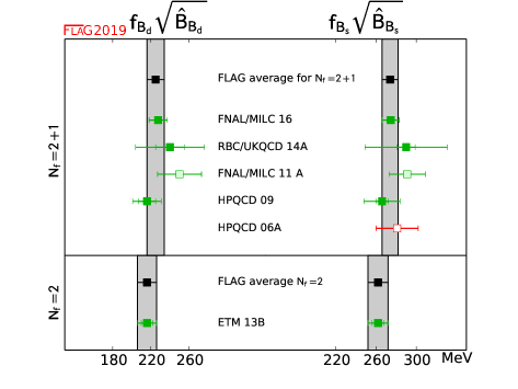
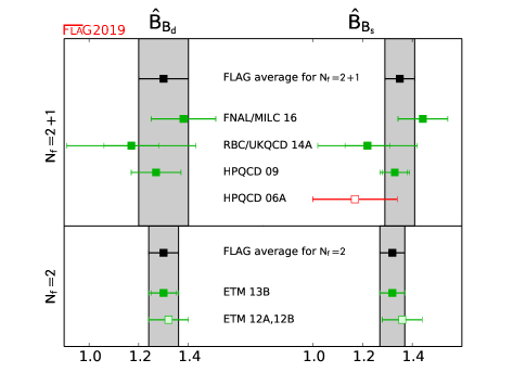
Figure 25: Neutral $B$- and $B_{\rm s}$-meson mixing matrix elements and bag parameters [values in Tab. 1 and Eqs. (216), (219), (217), (220)].

Collaboration	Ref.	$N_{f}$	publication status	continuum extrapolation	chiral extrapolation	finite volume	renormalization/matching	heavy-quark treatment	$\xi$	$B_{\rm B_{\rm s}}/B_{\rm B_{d}}$
FNAL/MILC 16	[Bazavov:2016nty]	2+1	A	$\bigstar$	$\circ$	$\bigstar$	$\circ$	✓	1.206(18)	1.033(31)(26)${}^{\odot}$
RBC/UKQCD 14A	[Aoki:2014nga]	2+1	A	$\circ$	$\circ$	$\circ$	$\circ$	✓	1.208(41)(52)	1.028(60)(49)
FNAL/MILC 12	[Bazavov:2012zs]	2+1	A	$\circ$	$\circ$	$\bigstar$	$\circ$	✓	1.268(63)	1.06(11)
RBC/UKQCD 10C	[Albertus:2010nm]	2+1	A	$\blacksquare$	$\blacksquare$	$\blacksquare$	$\circ$	✓	1.13(12)	$-$
HPQCD 09	[Gamiz:2009ku]	2+1	A	$\circ$	$\circ$${}^{\nabla}$	$\circ$	$\circ$	✓	1.258(33)	1.05(7)
ETM 13B	[Carrasco:2013zta]	2	A	$\bigstar$	$\circ$	$\circ$	$\bigstar$	✓	1.225(16)(14)(22)	1.007(15)(14)
ETM 12A, 12B	[Carrasco:2012dd, Carrasco:2012de]	2	C	$\bigstar$	$\circ$	$\circ$	$\bigstar$	✓	1.21(6)	1.03(2)

• PDG average of the ratio of decay constants $f_{B_{s}}/f_{B^{0}}$ [Rosner:2015wva] is used to obtain the value.
  

• Wrong-spin contributions are not included in the HMrS$\chi$PT fits. As the effect may not be negligible, these results are excluded from the average (see description in FLAG 13 [Aoki:2013ldr]).

Table 37: Results for $SU(3)$-breaking ratios of neutral $B_{d}$- and $B_{s}$-meson mixing matrix elements and bag parameters.

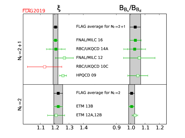
Figure 26: The $SU(3)$-breaking quantities $\xi$ and $B_{B_{s}}/B_{B_{d}}$ [values in Tab. 1 and Eqs. (218), (221)].

There are no new results for $N_{f}=2$ reported after the previous FLAG review. In this category one work (ETM 13B) [Carrasco:2013zta] passes the quality criteria. A description of this work can be found in the FLAG 13 review [Aoki:2013ldr] where it did not enter the average as it had not appeared in a journal. Because this is the only result available for $N_{f}=2$, we quote their values as our averages in this version:

$$f_{B_{d}}\sqrt{\hat{B}_{b_{d}}} =216(10)\;\;{\rm MeV} f_{B_{s}}\sqrt{\hat{B}_{B_{s}}} =262(10)\;\;{\rm MeV} \ref{~}\mbox{\cite[cite]{[\@@bibref{Number}{Carrasco:2013zta}{}{}]}},$$ (216)

$$N_{f}=2: \hat{B}_{B_{d}} =1.30(6) \hat{B}_{B_{s}} =1.32(5) \ref{~}\mbox{\cite[cite]{[\@@bibref{Number}{Carrasco:2013zta}{}{}]}},$$ (217)

$$\xi =1.225(31) B_{B_{s}}/B_{B_{d}} =1.007(21) \ref{~}\mbox{\cite[cite]{[\@@bibref{Number}{Carrasco:2013zta}{}{}]}}.$$ (218)

For the $N_{f}=2+1$ case the FNAL/MILC collaboration reported their new results on the neutral $B$-meson mixing parameters in 2016. As the paper [Bazavov:2016nty] appeared after the closing date of FLAG 16 [Aoki:2016frl], the results had not been taken into our average then. However, the subsequent web update of FLAG took the results into the average, and was made public in November 2017.

Their estimate of the $B^{0}-\overline{B^{0}}$ mixing matrix elements are far improved compared to their older ones as well as all the prior $N_{f}=2+1$ results. Hence, including the new FNAL/MILC results makes our averages much more precise. The study uses the asqtad action for light quarks and the Fermilab action for the $b$ quark. They use MILC asqtad ensembles spanning four lattice spacings in the range $a\approx 0.045-0.12$ fm and RMS pion mass of $257$ MeV as the lightest. The lightest Goldstone pion of 177 MeV, at which the RMS mass is 280 MeV, helps constraining the combined chiral and continuum limit analysis with the HMrS$\chi$PT (heavy-meson rooted-staggered chiral perturbation theory) to NLO with NNLO analytic terms using a Bayesian prior. The extension to the finer lattice spacing and closer to physical pion masses together with the quadrupled statistics of the ensembles compared with those used in the earlier studies, as well as the inclusion of the wrong spin contribution [Bernard:2013dfa], which is a staggered fermion artifact, make it possible to achieve the large improvement of the overall precision. Although for each parameter only one lattice volume is available, the finite-volume effects are well controlled by using a large enough lattice ($m_{\pi}^{\rm RMS}L\,\raisebox{-2.40002pt}{$\stackrel{{\scriptstyle\raisebox{-0.56003pt}{$>$}}}{{\sim}}$ }\,5$) for all the ensembles. The operator renormalization is done by 1-loop lattice perturbation theory with the help of the mostly nonperturbative renormalization method where a perturbative computation of the ratio of the four-quark operator and square of the vector-current renormalization factors is combined with the nonperturbative estimate of the latter. Let us note that in the report [Bazavov:2016nty] not only the SM $B^{0}-\overline{B^{0}}$ mixing matrix element, but also those with all possible four-quark operators are included. The correlation among the different matrix elements are given, which helps to properly assess the error propagation to phenomenological analyses where combinations of the different matrix elements enter. The authors estimate the effect of omitting the charm-quark dynamics, which we have not propagated to our $N_{f}=2+1$ averages. It should also be noted that their main new results are for the $B^{0}-\overline{B^{0}}$ mixing matrix elements, that are $f_{B_{d}}\sqrt{B_{B_{d}}}$, $f_{B_{s}}\sqrt{B_{B_{s}}}$ and the ratio $\xi$. They reported also on $B_{B_{d}}$, $B_{B_{s}}$ and $B_{B_{s}}/B_{B_{d}}$. However, the $B$-meson decay constants needed in order to isolate the bag parameters from the four-fermion matrix elements are taken from the PDG [Rosner:2015wva] averages, which are obtained using a procedure similar to that used by FLAG. They plan to compute the decay constants on the same gauge field ensembles and then complete the bag parameter calculation on their own in the future. As of now, for the bag parameters we need to use the nested averaging scheme, described in Sec. 2.3.2, to take into account the possible correlations with this new result to the other ones through the averaged decay constants. The detailed procedure to apply the scheme for this particular case is provided in Sec. 8.2.1.

The other results for $N_{f}=2+1$ are RBC/UKQCD 14A [Aoki:2014nga], which had been included in the averages at FLAG 16 [Aoki:2016frl], and HPQCD 09 [Gamiz:2009ku] to which a description is available in FLAG 13 [Aoki:2013ldr]. Now our averages for $N_{f}=2+1$ are:

$$f_{B_{d}}\sqrt{\hat{B}_{B_{d}}} =225(9)\,{\rm MeV} f_{B_{s}}\sqrt{\hat{B}_{B_{s}}} =274(8)\,{\rm MeV} \,\mathrm{Refs.}~{}\mbox{\cite[cite]{[\@@bibref{Number}{Gamiz:2009ku,Aoki:2014nga,Bazavov:2016nty}{}{}]}},$$ (219)

$$N_{f}=2+1: \hat{B}_{B_{d}} =1.30(10) \hat{B}_{B_{s}} =1.35(6) \,\mathrm{Refs.}~{}\mbox{\cite[cite]{[\@@bibref{Number}{Gamiz:2009ku,Aoki:2014nga,Bazavov:2016nty}{}{}]}},$$ (220)

$$\xi =1.206(17) B_{B_{s}}/B_{B_{d}} =1.032(38) \,\mathrm{Refs.}~{}\mbox{\cite[cite]{[\@@bibref{Number}{Aoki:2014nga,Bazavov:2016nty}{}{}]}}.$$ (221)

Here all the above equations have been updated from the paper version of FLAG 16. The new results from FNAL/MILC 16 [Bazavov:2016nty] entered the average for Eqs. (219), (220), and replaced the earlier FNAL/MILC 12 [Bazavov:2012zs] for Eq. (221).

As discussed in detail in the FLAG 13 review [Aoki:2013ldr] HPQCD 09 does not include wrong-spin contributions [Bernard:2013dfa], which are staggered fermion artifacts, to the chiral extrapolation analysis. It is possible that the effect is significant for $\xi$ and $B_{B_{s}}/B_{B_{d}}$, since the chiral extrapolation error is a dominant one for these flavour $SU(3)$-breaking ratios. Indeed, a test done by FNAL/MILC 12 [Bazavov:2012zs] indicates that the omission of the wrong spin contribution in the chiral analysis may be a significant source of error. We therefore took the conservative choice to exclude $\xi$ and $B_{B_{s}}/B_{B_{d}}$ by HPQCD 09 from our average and we follow the same strategy in this report as well.

We note that the above results within same $N_{f}$ are all correlated with each other, due to the use of the same gauge field ensembles for different quantities. The results are also correlated with the averages obtained in Sec. 8.1 and shown in Eqs. (196)–(198) for $N_{f}=2$ and Eqs. (199)–(201) for $N_{f}=2+1$, because the calculations of $B$-meson decay constants and mixing quantities are performed on the same (or on similar) sets of ensembles, and results obtained by a given collaboration use the same actions and setups. These correlations must be considered when using our averages as inputs to unitarity triangle (UT) fits. For this reason, if one were for example to estimate $f_{B_{s}}\sqrt{\hat{B}_{s}}$ from the separate averages of $f_{B_{s}}$ and $\hat{B}_{s}$, one would obtain a value about one standard deviation below the one quoted above. While these two estimates lead to compatible results, giving us confidence that all uncertainties have been properly addressed, we do not recommend combining averages this way, as many correlations would have to be taken into account to properly assess the errors. We recommend instead using the numbers quoted above. In the future, as more independent calculations enter the averages, correlations between the lattice-QCD inputs to UT fits will become less significant.

8.2.1 Error treatment for $B$-meson bag parameters

The latest FNAL/MILC computation (FNAL/MILC 16) uses $B$-meson decay constants averaged for PDG [Rosner:2015wva] to isolate the bag parameter from the mixing matrix elements. The bag parameters so obtained have correlation to those from the other computations in two ways: through the mixing matrix elements of FNAL/MILC 16 and through the PDG average. Since the PDG average is obtained similarly as the FLAG average, estimating the bag parameter average with FNAL/MILC 16 requires a nested scheme. The nested scheme discussed in Sec. 2.3.2 is applied as follows.

Three computations contribute to the $N_{f}=2+1$ average of the $B_{d}$ meson bag parameter $B_{B_{d}}$, FNAL/MILC 16 [Bazavov:2016nty], RBC/UKQCD 14A [Aoki:2014nga], HPQCD 09 [Gamiz:2009ku]. FNAL/MILC 16 uses $f_{B^{0}}$ of PDG [Rosner:2015wva], which is an average of RBC/UKQCD 14, RBC/UKQCD 14A, HPQCD 12/11A, FNAL/MILC 11 in Tab. 1. $B_{B_{d}}$ (RBC/UKQCD 14A) has correlation with that of FNAL/MILC 16, through $f_{B}$ (RBC/UKQCD 14A). Also some correlation exists through $f_{B}$ (RBC/UKQCD 14), which uses the same set of gauge field configurations as $B_{B_{d}}$ (RBC/UKQCD 14A).

In Eq. (9) for this particular case, $Q_{1}$ is $B_{B_{d}}$ (FNAL/MILC 16), $Y_{1}$ is $f_{B^{0}}^{2}B_{B_{d}}$ (FNAL/MILC 16), and $\overline{Z}$ is the PDG average of $f_{B^{0}}^{2}$. The most nontrivial part of the nested averaging is to construct the restricted errors $\sigma[f_{B}^{2}]_{i^{\prime}\leftrightarrow k}$ [Eq. (16)] and $\sigma[f_{B}^{2}]_{i^{\prime};j^{\prime}\leftrightarrow k}$ [Eq. (18)], which goes into the final correlation matrix $C_{ij}$ of $B_{B_{d}}$ through $\sigma_{1;k}$ [Eq. (14)]. The restricted summation over $(\alpha)$ labeling the origin of errors in this analysis turns out to be either the whole error or the statistical error only.

For the correlation of $f_{B}$ and $B_{B_{d}}$ both with RBC/UKQCD 14A, not knowing the information of the correlation, we take total errors 100 % correlated. For example, the heavy-quark error, which is $O(1/m_{b})$ and most dominant, is common for both. For the correlation of $f_{B}$ (RBC/UKQCD 14) and $B_{B_{d}}$ (RBC/UKQCD 14A), which uses different heavy-quark formulations but based on the same set of gauge field configurations, only the statistical error is taken as correlated. In a similar way, correlation among the other computations is determined. In principle, we take the whole error as correlated between $f_{B}$ and $B_{B_{d}}$ if both results are based on the exact same lattice action for light and heavy quarks and are sharing (at least a part of) the gauge field ensemble. Otherwise, only the statistical error is taken as correlated if two computations share the gauge field ensemble, or no correlation for the rest, which is summarized in Tab. 38. Also in a similar way, correlations of $f_{B_{s}}$ and $B_{B_{s}}$, $f_{B_{s}}/f_{B}$ and $B_{B_{s}}/B_{B_{d}}$ are determined, which are also summarized in Tab. 38.

The necessary information for constructing the second term in the square root of Eq. (14) has already been provided. For completeness, let us also summarize the correlation pattern needed to construct the other part of $\sigma_{i;j}$ for the bag parameters, which is shown in Tab. 39.

$\sigma[Z]_{i^{\prime};j^{\prime}\leftrightarrow k}$ for $k=$[RBC/UKQCD 14A]
$i^{\prime}\;\backslash\;j^{\prime}$	RBC/UKQCD 14A	RBC/UKQCD 14
RBC/UKQCD 14A	all	stat
RBC/UKQCD 14	stat	stat

$\sigma[f_{B}^{2}]_{i^{\prime};j^{\prime}\leftrightarrow k}$ for $k=$[HPQCD 09]
$i^{\prime}\;\backslash\;j^{\prime}$	HPQCD 12/11A	FNAL/MILC 11
HPQCD 12/11A	all	stat
FNAL/MILC 11	stat	stat

$\sigma[f_{B_{s}}^{2}]_{i^{\prime};j^{\prime}\leftrightarrow k}$ for $k=$[HPQCD 09]
$i^{\prime}\;\backslash\;j^{\prime}$	HPQCD 12	HPQCD 11A	FNAL/MILC 11
HPQCD 12	all	stat	stat
HPQCD 11A	stat	stat	stat
FNAL/MILC 11	stat	stat	stat

Table 38: Correlated elements of error composition in the summation over $(\alpha)$ for $\sigma[Z]_{i^{\prime};j^{\prime}\leftrightarrow k}$ [Eq. (18)] for $Z=f_{B}^{2},f_{B_{s}}^{2},f_{B_{s}}^{2}/f_{B}^{2}$. The $i^{\prime}=j^{\prime}$ elements express $\sigma[Z]_{i^{\prime}\leftrightarrow k}$ [Eq. (16)]. The elements not listed here are all null.

$i\;\backslash\;j$	FNAL/MILC 16	RBC/UKQCD 14A	HPQCD 09
FNAL/MILC 16	$-$	none	stat
RBC/UKQCD 14A	all	$-$	none
HPQCD 09	all	none	$-$

Table 39: Correlated elements of error composition in the summation over $(\alpha)$ for $\sigma_{i;j}$ of $B_{B_{d}}$, $B_{B_{s}}$, $B_{B_{s}}/B_{B_{d}}$. The $i=$[FNAL/MILC 16] row expresses the correlations in the first term in the square root in Eq. (14). The $j=$[FNAL/MILC 16] column represents the correlations for Eq. (19). For $B_{B_{s}}/B_{B_{d}}$ only upper $2\times 2$ block is relevant.

8.3 Semileptonic form factors for $B$ decays to light flavours

The Standard Model differential rate for the decay $B_{(s)}\to P\ell\nu$ involving a quark-level $b\to u$ transition is given, at leading order in the weak interaction, by a formula analogous to the one for $D$ decays in Eq. (171), but with $D\to B_{(s)}$ and the relevant CKM matrix element $|V_{cq}|\to|V_{ub}|$:

$$\hbox{$d\Gamma(B_{(s)}\to P\ell\nu)\over dq^{2}$}=\hbox{$G_{F}^{2}|V_{ub}|^{2}\over 24\pi^{3}$}\,\hbox{$(q^{2}-m_{\ell}^{2})^{2}\sqrt{E_{P}^{2}-m_{P}^{2}}\over q^{4}m_{B_{(s)}}^{2}$}{\hbox{$\left[\vbox to0.0pt{}\right.\n@space$}} \!\!\!\!\!\!\!\!\!\!\!\left(1+\hbox{$m_{\ell}^{2}\over 2q^{2}$}\right)m_{B_{(s)}}^{2}(E_{P}^{2}-m_{P}^{2})|f_{+}(q^{2})|^{2}$$ (222)

$$~{}~{}~{}~{}\,+\,\hbox{$3m_{\ell}^{2}\over 8q^{2}$}(m_{B_{(s)}}^{2}-m_{P}^{2})^{2}|f_{0}(q^{2})|^{2}{\hbox{$\left]\vbox to0.0pt{}\right.\n@space$}}\,.$$

Again, for $\ell=e,\mu$ the contribution from the scalar form factor $f_{0}$ can be neglected, and one has a similar expression to Eq. (173), which, in principle, allows for a direct extraction of $|V_{ub}|$ by matching theoretical predictions to experimental data. However, while for $D$ (or $K$) decays the entire physical range $0\leq q^{2}\leq q^{2}_{\rm max}$ can be covered with moderate momenta accessible to lattice simulations, in $B\to\pi\ell\nu$ decays one has $q^{2}_{\rm max}\sim 26~{}{\rm GeV}^{2}$ and only part of the full kinematic range is reachable. As a consequence, obtaining $|V_{ub}|$ from $B\to\pi\ell\nu$ is more complicated than obtaining $|V_{cd(s)}|$ from semileptonic $D$-meson decays.

In practice, lattice computations are restricted to large values of the momentum transfer $q^{2}$ (see Sec. 7.2) where statistical and momentum-dependent discretization errors can be controlled, which in existing calculations roughly cover the upper third of the kinematically allowed $q^{2}$ range. Since, on the other hand, the decay rate is suppressed by phase space at large $q^{2}$, most of the semileptonic $B\to\pi$ events are selected in experiment at lower values of $q^{2}$, leading to more accurate experimental results for the binned differential rate in that region. It is therefore a challenge to find a window of intermediate values of $q^{2}$ at which both the experimental and lattice results can be reliably evaluated.

In current practice, the extraction of CKM matrix elements requires that both experimental and lattice data for the $q^{2}$-dependence be parameterized by fitting data to a specific ansatz. Before the generalization of the sophisticated ansätze that will be discussed below, the most common procedure to overcome this difficulty involved matching the theoretical prediction and the experimental result for the integrated decay rate over some finite interval in $q^{2}$,

$$\Delta\zeta=\hbox{$1\over|V_{ub}|^{2}$}\int_{q^{2}_{1}}^{q^{2}_{2}}\left(\hbox{$d\Gamma\over dq^{2}$}\right)dq^{2}\,.$$ (223)

In the most recent literature, it has become customary to perform a joint fit to lattice and experimental results, keeping the relative normalization $|V_{ub}|^{2}$ as a free parameter. In either case, good control of the systematic uncertainty induced by the choice of parameterization is crucial to obtain a precise determination of $|V_{ub}|$. A detailed discussion of the parameterization of form factors as a function of $q^{2}$ can be found in Appendix LABEL:sec:zparam.

8.3.1 Form factors for $B\to\pi\ell\nu$

The semileptonic decay processes $B\to\pi\ell\nu$ enable determinations of the CKM matrix element $|V_{ub}|$ within the Standard Model via Eq. (222). Early results for $B\to\pi\ell\nu$ form factors came from the HPQCD [Dalgic:2006dt] and FNAL/MILC [Bailey:2008wp] collaborations. Only HPQCD provided results for the scalar form factor $f_{0}$. Our previous review featured a significantly extended calculation of $B\to\pi\ell\nu$ from FNAL/MILC [Lattice:2015tia] and a new computation from RBC/UKQCD [Flynn:2015mha]. All the above computations employ $N_{f}=2+1$ dynamical configurations, and provide values for both form factors $f_{+}$ and $f_{0}$. In addition, HPQCD using MILC ensembles had published the first $N_{f}=2+1+1$ results for the $B\to\pi\ell\nu$ scalar form factor, working at zero recoil and pion masses down to the physical value [Colquhoun:2015mfa]; this adds to previous reports on ongoing work to upgrade their 2006 computation [Bouchard:2012tb, Bouchard:2013zda]. Since this latter result has no immediate impact on current $|V_{ub}|$ determinations, which come from the vector-form-factor-dominated decay channels into light leptons, we will from now on concentrate on the $N_{f}=2+1$ determinations of the $q^{2}$-dependence of $B\to\pi$ form factors.

Results presented at Lattice 2017 are preliminary or blinded, so not yet ready for inclusion in this review. However, the reader will be interested to know that the JLQCD collaboration is using Möbius Domain Wall fermions with $a\approx 0.08$, 0.055, and 0.044 fm and pion masses down to 300 MeV to study this process [Colquhoun:2017gfi]. FNAL/MILC is using $N_{f}=2+1+1$ HISQ ensembles with $a\approx 0.15$, 0.12, and 0.088 fm, with Goldstone pion mass down to its physical value [Gelzer:2017edb]. Both groups updated their results for Lattice 2018, but do not have final values for the form factors.

Returning to the works that contribute to our averages, both the HPQCD and the FNAL/MILC computations of $B\to\pi\ell\nu$ amplitudes use ensembles of gauge configurations with $N_{f}=2+1$ flavours of rooted staggered quarks produced by the MILC collaboration; however, the latest FNAL/MILC work makes a much more extensive use of the currently available ensembles, both in terms of lattice spacings and light-quark masses. HPQCD have results at two values of the lattice spacing ($a\sim 0.12,~{}0.09~{}{\rm fm}$), while FNAL/MILC employs four values ($a\sim 0.12,~{}0.09,~{}0.06,~{}0.045~{}{\rm fm}$). Lattice-discretization effects are estimated within HMrS$\chi$PT in the FNAL/MILC computation, while HPQCD quotes the results at $a\sim 0.12~{}{\rm fm}$ as central values and uses the $a\sim 0.09~{}{\rm fm}$ results to quote an uncertainty. The relative scale is fixed in both cases through $r_{1}/a$. HPQCD set the absolute scale through the $\Upsilon$ $2S$–$1S$ splitting, while FNAL/MILC uses a combination of $f_{\pi}$ and the same $\Upsilon$ splitting, as described in Ref. [Bazavov:2011aa]. The spatial extent of the lattices employed by HPQCD is $L\simeq 2.4~{}{\rm fm}$, save for the lightest mass point (at $a\sim 0.09~{}{\rm fm}$) for which $L\simeq 2.9~{}{\rm fm}$. FNAL/MILC, on the other hand, uses extents up to $L\simeq 5.8~{}{\rm fm}$, in order to allow for light-pion masses while keeping finite-volume effects under control. Indeed, while in the 2006 HPQCD work the lightest RMS pion mass is $400~{}{\rm MeV}$, the latest FNAL/MILC work includes pions as light as $165~{}{\rm MeV}$—in both cases the bound $m_{\pi}L\gtrsim 3.8$ is kept. Other than the qualitatively different range of MILC ensembles used in the two computations, the main difference between HPQCD and FNAL/MILC lies in the treatment of heavy quarks. HPQCD uses the NRQCD formalism, with a 1-loop matching of the relevant currents to the ones in the relativistic theory. FNAL/MILC employs the clover action with the Fermilab interpretation, with a mostly nonperturbative renormalization of the relevant currents, within which light-light and heavy-heavy currents are renormalized nonperturbatively and 1-loop perturbation theory is used for the relative normalization. (See Tab. 1; full details about the computations are provided in tables in Appendix LABEL:app:BtoPi_Notes.)

The RBC/UKQCD computation is based on $N_{f}=2+1$ DWF ensembles at two values of the lattice spacing ($a\sim 0.12,~{}0.09~{}{\rm fm}$), and pion masses in a narrow interval ranging from slightly above $400~{}{\rm MeV}$ to slightly below $300~{}{\rm MeV}$, keeping $m_{\pi}L\gtrsim 4$. The scale is set using the $\Omega^{-}$ baryon mass. Discretization effects coming from the light sector are estimated in the $1\%$ ballpark using HM$\chi$PT supplemented with effective higher-order interactions to describe cutoff effects. The $b$ quark is treated using the Columbia RHQ action, with a mostly nonperturbative renormalization of the relevant currents. Discretization effects coming from the heavy sector are estimated with power-counting arguments to be below $2\%$.

Given the large kinematical range available in the $B\to\pi$ transition, chiral extrapolations are an important source of systematic uncertainty: apart from the eventual need to reach physical pion masses in the extrapolation, the applicability of $\chi$PT is not guaranteed for large values of the pion energy $E_{\pi}$. Indeed, in all computations $E_{\pi}$ reaches values in the $1~{}{\rm GeV}$ ballpark, and chiral extrapolation systematics is the dominant source of errors. FNAL/MILC uses $SU(2)$ NLO HMrS$\chi$PT for the continuum-chiral extrapolation, supplemented by NNLO analytic terms and hard-pion $\chi$PT terms [Bijnens:2010ws]; systematic uncertainties are estimated through an extensive study of the effects of varying the specific fit ansatz and/or data range. RBC/UKQCD uses $SU(2)$ hard-pion HM$\chi$PT to perform its combined continuum-chiral extrapolation, and obtains sizeable estimates for systematic uncertainties by varying the ansätze and ranges used in fits. HPQCD performs chiral extrapolations using HMrS$\chi$PT formulae, and estimates systematic uncertainties by comparing the result with the ones from fits to a linear behaviour in the light-quark mass, continuum HM$\chi$PT, and partially quenched HMrS$\chi$PT formulae (including also data with different sea and valence light-quark masses).

FNAL/MILC and RBC/UKQCD describe the $q^{2}$-dependence of $f_{+}$ and $f_{0}$ by applying a BCL parameterization to the form factors extrapolated to the continuum limit, within the range of values of $q^{2}$ covered by data. RBC/UKQCD generate synthetic data for the form factors at some values of $q^{2}$ (evenly spaced in $z$) from the continuous function of $q^{2}$ obtained from the joint chiral-continuum extrapolation, which are then used as input for the fits. After having checked that the kinematical constraint $f_{+}(0)=f_{0}(0)$ is satisfied within errors by the extrapolation to $q^{2}=0$ of the results of separate fits, this constraint is imposed to improve fit quality. In the case of FNAL/MILC, rather than producing synthetic data a functional method is used to extract the $z$-parameterization directly from the fit functions employed in the continuum-chiral extrapolation. In the case of HPQCD, the parameterization of the $q^{2}$-dependence of form factors is somewhat intertwined with chiral extrapolations: a set of fiducial values $\{E_{\pi}^{(n)}\}$ is fixed for each value of the light-quark mass, and $f_{+,0}$ are interpolated to each of the $E_{\pi}^{(n)}$; chiral extrapolations are then performed at fixed $E_{\pi}$ (i.e., $m_{\pi}$ and $q^{2}$ are varied subject to $E_{\pi}$=constant). The interpolation is performed using a BZ ansatz. The $q^{2}$-dependence of the resulting form factors in the chiral limit is then described by means of a BZ ansatz, which is cross-checked against BK, RH, and BGL parameterizations. Unfortunately, the correlation matrix for the values of the form factors at different $q^{2}$ is not provided, which severely limits the possibilities of combining them with other computations into a global $z$-parameterization.

Based on the parameterized form factors, HPQCD and RBC/UKQCD provide values for integrated decay rates $\Delta\zeta^{B\pi}$, as defined in Eq. (223); they are quoted in Tab. 1. The latest FNAL/MILC work, on the other hand, does not quote a value for the integrated ratio. Furthermore, as mentioned above, the field has recently moved forward to determine CKM matrix elements from direct joint fits of experimental results and theoretical form factors, rather than a matching through $\Delta\zeta^{B\pi}$. Thus, we will not provide here a FLAG average for the integrated rate, and focus on averaging lattice results for the form factors themselves.

Collaboration	Ref.	$N_{f}$	publication status	continuum extrapolation	chiral extrapolation	finite volume	renormalization	heavy-quark treatment	$z$-parameterization	$\Delta\zeta^{B\pi}$
FNAL/MILC 15	[Lattice:2015tia]	2+1	A	$\bigstar$	$\circ$	$\bigstar$	$\circ$	✓	BCL	n/a
RBC/UKQCD 15	[Flynn:2015mha]	2+1	A	$\circ$	$\circ$	$\circ$	$\circ$	✓	BCL	$\quad 1.77(34)$
HPQCD 06	[Dalgic:2006dt]	2+1	A	$\circ$	$\circ$	$\circ$	$\circ$	✓	n/a	2.07(41)(39)

Table 40: Results for the $B\to\pi\ell\nu$ semileptonic form factor. The quantity $\Delta\zeta$ is defined in Eq. (223); the quoted values correspond to $q_{1}=4$ GeV, $q_{2}=q_{max}$, and are given in $\mbox{ps}^{-1}$.

The different ways in which the current results are presented do not allow a straightforward averaging procedure. RBC/UKQCD only provides synthetic values of $f_{+}$ and $f_{0}$ at a few values of $q^{2}$ as an illustration of their results, and FNAL/MILC does not quote synthetic values at all. In both cases, full results for BCL $z$-parameterizations defined by Eq. (LABEL:eq:bcl_c) are quoted. In the case of HPQCD 06, unfortunately, a fit to a BCL $z$-parameterization is not possible, as discussed above.

In order to combine these form factor calculations we start from sets of synthetic data for several $q^{2}$ values. HPQCD and RBC/UKQCD provide directly this information; FNAL/MILC presents only fits to a BCL $z$-parameterization from which we can easily generate an equivalent set of form factor values. It is important to note that in both the RBC/UKQCD synthetic data and the FNAL/MILC $z$-parameterization fits the kinematic constraint at $q^{2}=0$ is automatically included (in the FNAL/MILC case the constraint is manifest in an exact degeneracy of the $(a_{n}^{+},a_{n}^{0})$ covariance matrix). Due to these considerations, in our opinion the most accurate procedure is to perform a simultaneous fit to all synthetic data for the vector and scalar form factors. Unfortunately, the absence of information on the correlation in the HPQCD result between the vector and scalar form factors even at a single $q^{2}$ point makes it impossible to include consistently this calculation in the overall fit. In fact, the HPQCD and FNAL/MILC statistical uncertainties are highly correlated (because they are based on overlapping subsets of MILC $N_{f}=2+1$ ensembles) and, without knowledge of the $f_{+}-f_{0}$ correlation we are unable to construct the HPQCD-FNAL/MILC off-diagonal entries of the overall covariance matrix.

In conclusion, we will present as our best result a combined vector and scalar form factor fit to the FNAL/MILC and RBC/UKQCD results that we treat as completely uncorrelated. For sake of completeness we will also show the results of a vector form factor fit alone in which we include one HPQCD datum at $q^{2}=17.34~{}\,\mathrm{GeV}^{2}$ assuming conservatively a 100% correlation between the statistical error of this point and of all FNAL/MILC synthetic data. In spite of contributing just one point, the HPQCD datum has a significant weight in the fit due to its small overall uncertainty. We stress again that this procedure is slightly inconsistent because FNAL/MILC and RBC/UKQCD include information on the kinematic constraint at $q^{2}=0$ in their $f_{+}$ results.

The resulting data set is then fitted to the BCL parameterization in Eqs. (LABEL:eq:bcl_c) and (LABEL:eq:bcl_f0). We assess the systematic uncertainty due to truncating the series expansion by considering fits to different orders in $z$. In Fig. 27, we show the FNAL/MILC, RBC/UKQCD, and HPQCD data points for $(1-q^{2}/m_{B^{*}}^{2})f_{+}(q^{2})$ and $f_{0}(q^{2})$ versus $z$. The data is highly linear and we get a good $\chi^{2}/{\rm dof}$ with $N^{+}=N^{0}=3$. Note that this implies three independent parameters for $f_{+}$ corresponding to a polynomial through $\mathcal{O}(z^{3})$ and two independent parameters for $f_{0}$ corresponding to a polynomial through $\mathcal{O}(z^{2})$ (the coefficient $a_{2}^{0}$ is fixed using the $q^{2}=0$ kinematic constraint). We cannot constrain the coefficients of the $z$-expansion beyond this order; for instance, including a fourth parameter in $f_{+}$ results in 100% uncertainties on $a_{2}^{+}$ and $a_{3}^{+}$. The outcome of the five-parameter $N^{+}=N^{0}=3$ BCL fit to the FNAL/MILC and RBC/UKQCD calculations is shown in Tab. 41. The uncertainties on $a_{0}^{+,0}$, $a_{1}^{+,0}$ and $a_{2}^{+}$ encompass the central values obtained from $N^{+}=2,4$ and $N^{0}=2,4,5$ fits and thus adequately reflect the systematic uncertainty on those series coefficients. This can be used as the averaged FLAG result for the lattice-computed form factor $f_{+}(q^{2})$. The coefficient $a_{3}^{+}$ can be obtained from the values for $a_{0}^{+}$–$a_{2}^{+}$ using Eq. (LABEL:eq:red_coeff). The coefficient $a_{2}^{0}$ can be obtained from all other coefficients imposing the $f_{+}(q^{2}=0)=f_{0}(q^{2}=0)$ constraint. The fit is illustrated in Fig. 27.

$B\to\pi\;(N_{f}=2+1)$
	Central Values	Correlation Matrix
$a_{0}^{+}$	0.404 (13)	1	0.404	0.118	0.327	0.344
$a_{1}^{+}$	$-$0.68 (13)	0.404	1	0.741	0.310	0.900
$a_{2}^{+}$	$-$0.86 (61)	0.118	0.741	1	0.363	0.886
$a_{0}^{0}$	0.490 (21)	0.327	0.310	0.363	1	0.233
$a_{1}^{0}$	$-$1.61 (16)	0.344	0.900	0.886	0.233	1

Table 41: Coefficients and correlation matrix for the $N^{+}=N^{0}=3$ $z$-expansion of the $B\to\pi$ form factors $f_{+}$ and $f_{0}$.

It is worth stressing that, with respect to our average in the 2015 edition of the FLAG report, the relative error on $a_{0}^{+}$, which dominates the theory contribution to the determination of $|V_{ub}|$, has decreased from $7.3\%$ to $3.2\%$. The dominant factor in this remarkable improvement is the new FNAL/MILC determination of $f_{+}$. We emphasize that future lattice-QCD calculations of semileptonic form factors should publish their full statistical and systematic correlation matrices to enable others to use the data. It is also preferable to present a set of synthetic form factors data equivalent to the $z$-fit results, since this allows for an independent analysis that avoids further assumptions about the compatibility of the procedures to arrive at a given $z$-parameterization. It is also preferable to present covariance/correlation matrices with enough significant digits to calculate correctly all their eigenvalues.

For the sake of completeness, we present also a standalone $z$-fit to the vector form factor. In this fit we are able to include the single $f_{+}$ point at $q^{2}=17.34\;{\rm GeV}^{2}$ that we mentioned above. This fit uses the FNAL/MILC and RBC/UKQCD results that do make use of the kinematic constraint at $q^{2}=0$, but is otherwise unbiased. The results of the three-parameter BCL fit to the HPQCD, FNAL/MILC and RBC/UKQCD calculations of the vector form factor are:

$$N_{f}=2+1:\qquad a_{0}^{+}=0.421(13)\,,~{}~{}~{}~{}a_{1}^{+}=-0.35(10)\,,~{}~{}~{}~{}a_{2}^{+}=-0.41(64)\,;$$ (224)

$$\qquad\qquad{\rm corr}(a_{i},a_{j})=\left(\begin{array}[]{rrr}1.000&0.306&0.084\\ 0.306&1.000&0.856\\ 0.084&0.856&1.000\end{array}\right)\,.$$ (228)

Note that the $a_{0}^{+}$ coefficient, that is the most relevant for input to the extraction of $V_{ub}$ from semileptonic $B\to\pi\ell\nu_{\ell}(\ell=e,\mu)$ decays, shifts by about a standard deviation.

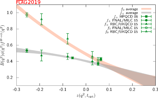
Figure 27: The form factors $(1-q^{2}/m_{B^{*}}^{2})f_{+}(q^{2})$ and $f_{0}(q^{2})$ for $B\to\pi\ell\nu$ plotted versus $z$. (See text for a discussion of the data set.) The grey and salmon bands display our preferred $N^{+}=N^{0}=3$ BCL fit (five parameters) to the plotted data with errors.

8.3.2 Form factors for $B_{s}\to K\ell\nu$

Similar to $B\to\pi\ell\nu$, measurements of $B_{s}\to K\ell\nu$ enable determinations of the CKM matrix element $|V_{ub}|$ within the Standard Model via Eq. (222). From the lattice point of view the two channels are very similar—as a matter of fact, $B_{s}\to K\ell\nu$ is actually somewhat simpler, in that the fact that the kaon mass region is easily accessed by all simulations makes the systematic uncertainties related to chiral extrapolation smaller. On the other hand, $B_{s}\to K\ell\nu$ channels have not been measured experimentally yet, and therefore lattice results provide SM predictions for the relevant rates.

At the time of our previous review, results for $B_{s}\to K\ell\nu$ form factors were provided by HPQCD [Bouchard:2014ypa] and RBC/UKQCD [Lattice:2015tia] for both form factors $f_{+}$ and $f_{0}$, in both cases using $N_{f}=2+1$ dynamical configurations. The ALPHA collaboration determination of $B_{s}\to K\ell\nu$ form factors with $N_{f}=2$ was also well underway [Bahr:2014iqa]; however, we have not seen final results. HPQCD has recently emphasized the value of form factor ratios for the processes $B_{s}\to K\ell\nu$ and $B_{s}\to D_{s}\ell\nu$ for determination of $|V_{ub}/V_{cb}|$ [Monahan:2018lzv]. Preliminary results from FNAL/MILC have been reported for $N_{f}=2+1$ [Lattice:2017vqf] and $N_{f}=2+1+1$ [Gelzer:2017edb]. Archival papers are expected soon.

The RBC/UKQCD computation has been published together with the $B\to\pi\ell\nu$ computation discussed in Sec. 8.3.1, all technical details being practically identical. The main difference is that errors are significantly smaller, mostly due to the reduction of systematic uncertainties due to the chiral extrapolation; detailed information is provided in tables in Appendix LABEL:app:BtoPi_Notes. The HPQCD computation uses ensembles of gauge configurations with $N_{f}=2+1$ flavours of asqtad rooted staggered quarks produced by the MILC collaboration at two values of the lattice spacing ($a\sim 0.12,~{}0.09~{}{\rm fm}$), for three and two different sea-pion masses, respectively, down to a value of $260~{}{\rm MeV}$. The $b$ quark is treated within the NRQCD formalism, with a 1-loop matching of the relevant currents to the ones in the relativistic theory, omitting terms of $\mathcal{O}(\alpha_{s}\Lambda_{\rm QCD}/m_{b})$. The HISQ action is used for the valence $s$ quark. The continuum-chiral extrapolation is combined with the description of the $q^{2}$-dependence of the form factors into a modified $z$-expansion (cf. Appendix LABEL:sec:zparam) that formally coincides in the continuum with the BCL ansatz. The dependence of form factors on the pion energy and quark masses is fitted to a 1-loop ansatz inspired by hard-pion $\chi$PT [Bijnens:2010ws], that factorizes out the chiral logarithms describing soft physics. See Tab. 1 and the tables in Appendix LABEL:app:BtoPi_Notes for full details.

Collaboration	Ref.	$N_{f}$	publication status	continuum extrapolation	chiral extrapolation	finite volume	renormalization	heavy-quark treatment	$z$-parameterization
RBC/UKQCD 15	[Flynn:2015mha]	2+1	A	$\circ$	$\circ$	$\circ$	$\circ$	✓	BCL
HPQCD 14	[Bouchard:2014ypa]	2+1	A	$\circ$	$\circ$	$\circ$	$\circ$	✓	BCL${}^{\dagger}$

• Results from modified $z$-expansion.

Table 42: Results for the $B_{s}\to K\ell\nu$ semileptonic form factor.

Both RBC/UKQCD and HPQCD quote values for integrated differential decay rates over the full kinematically available region. However, since the absence of experiment makes the relevant integration interval subject to change, we will not discuss them here, and focus on averages of form factors. In order to combine the results from the two collaborations, we will follow a similar approach to the one adopted above for $B\to\pi\ell\nu$: we will take as direct input the synthetic values of the form factors provided by RBC/UKQCD, use the preferred HPQCD parameterization to produce synthetic values, and perform a joint fit to the two data sets.

Note that the kinematic constraint at $q^{2}=0$ is included explicitly in the results presented by HPQCD (the coefficient $b_{0}^{0}$ is expressed analytically in terms of all others) and implicitly in the synthetic data provided by RBC/UKQCD. Therefore, following the procedure we adopted for the $B\to\pi$ case, we present a joint fit to the vector and scalar form factors and implement explicitly the $q^{2}=0$ constraint by expressing the coefficient $b^{0}_{N^{0}-1}$ in terms of all others.

For the fits we employ a BCL ansatz with $t_{+}=(M_{B_{s}}+M_{K^{\pm}})^{2}\simeq 34.35~{}\,\mathrm{GeV}^{2}$ and $t_{0}=(M_{B_{s}}+M_{K^{\pm}})(\sqrt{M_{B_{s}}}-\sqrt{M_{K^{\pm}}})^{2}\simeq 15.27~{}\,\mathrm{GeV}^{2}$. Our pole factors will contain a single pole in both the vector and scalar channels, for which we take the mass values $M_{B^{*}}=5.325~{}\,\mathrm{GeV}$ and $M_{B^{*}(0^{+})}=5.65~{}\,\mathrm{GeV}$.

The outcome of the five-parameter $N^{+}=N^{0}=3$ BCL fit, which we quote as our preferred result, is shown in Tab. 43. The uncertainties on $a_{0}$ and $a_{1}$ encompass the central values obtained from $\mathcal{O}(z^{2})$ fits, and thus adequately reflect the systematic uncertainty on those series coefficients. These can be used as the averaged FLAG results for the lattice-computed form factors $f_{+}(q^{2})$ and $f_{0}(q^{2})$. The coefficient $a_{3}^{+}$ can be obtained from the values for $a_{0}^{+}$–$a_{2}^{+}$ using Eq. (LABEL:eq:red_coeff). The fit is illustrated in Fig. 28.

$B_{s}\to K\;(N_{f}=2+1)$
	Central Values	Correlation Matrix
$a_{0}^{+}$	0.360(14)	1	0.098	$-$0.216	0.730	0.345
$a_{1}^{+}$	$-$0.828(83)	0.098	1	0.459	0.365	0.839
$a_{2}^{+}$	1.11(55)	$-$0.216	0.459	1	0.263	0.6526
$a_{0}^{0}$	0.233(10)	0.730	0.365	0.263	1	0.506
$a_{1}^{0}$	0.197(81)	0.345	0.839	0.652	0.506	1

Table 43: Coefficients and correlation matrix for the $N^{+}=N^{0}=3$ $z$-expansion of the $B_{s}\to K$ form factors $f_{+}$ and $f_{0}$.

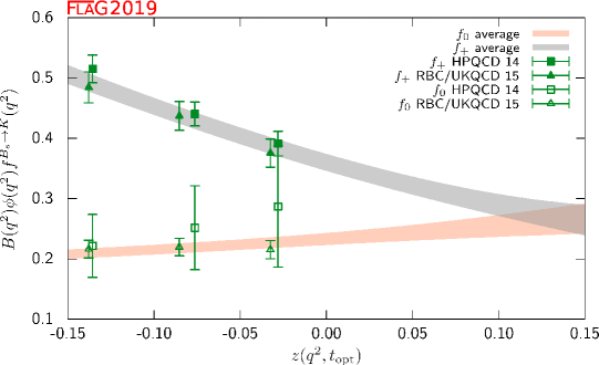
Figure 28: The form factors $(1-q^{2}/m_{B^{*}}^{2})f_{+}(q^{2})$ and $(1-q^{2}/m_{B^{*}(0+)}^{2})f_{0}(q^{2})$ for $B_{s}\to K\ell\nu$ plotted versus $z$. (See text for a discussion of the data sets.) The grey and salmon bands display our preferred $N^{+}=N^{0}=3$ BCL fit (five parameters) to the plotted data with errors.

8.3.3 Form factors for rare and radiative $B$-semileptonic decays to light flavours

Lattice-QCD input is also available for some exclusive semileptonic decay channels involving neutral-current $b\to q$ transitions at the quark level, where $q=d,s$. Being forbidden at tree level in the SM, these processes allow for stringent tests of potential new physics; simple examples are $B\to K^{*}\gamma$, $B\to K^{(*)}\ell^{+}\ell^{-}$, or $B\to\pi\ell^{+}\ell^{-}$ where the $B$ meson (and therefore the light meson in the final state) can be either neutral or charged.

The corresponding SM effective weak Hamiltonian is considerably more complicated than the one for the tree-level processes discussed above: after integrating out the top and the W boson, as many as ten dimension-six operators formed by the product of two hadronic currents or one hadronic and one leptonic current appear. Three of the latter, coming from penguin and box diagrams, dominate at short distances and have matrix elements that, up to small QED corrections, are given entirely in terms of $B\to(\pi,K,K^{*})$ form factors. The matrix elements of the remaining seven operators can be expressed, up to power corrections whose size is still unclear, in terms of form factors, decay constants and light-cone distribution amplitudes (for the $\pi$, $K$, $K^{*}$ and $B$ mesons) by employing OPE arguments (at large di-lepton invariant mass) and results from Soft Collinear Effective Theory (at small di-lepton invariant mass). In conclusion, the most important contributions to all of these decays are expected to come from matrix elements of current operators (vector, tensor, and axial-vector) between one-hadron states, which in turn can be parameterized in terms of a number of form factors (see Ref. [Liu:2009dj] for a complete description).

Collaboration	Ref.	$N_{f}$	publication status	continuum extrapolation	chiral extrapolation	finite volume	renormalization	heavy-quark treatment	$z$-parameterization
HPQCD 13E	[Bouchard:2013pna]	2+1	A	$\circ$	$\circ$	$\circ$	$\circ$	✓	BCL
FNAL/MILC 15D	[Bailey:2015dka]	2+1	A	$\bigstar$	$\circ$	$\bigstar$	$\circ$	✓	BCL

Table 44: Results for the $B\to K$ semileptonic form factors.

In channels with pseudoscalar mesons in the final state, the level of sophistication of lattice calculations is similar to the $B\to\pi$ case and there are results for the vector, scalar, and tensor form factors for $B\to K\ell^{+}\ell^{-}$ decays by HPQCD [Bouchard:2013pna], and more recent results for both $B\to\pi\ell^{+}\ell^{-}$ [Bailey:2015nbd] and $B\to K\ell^{+}\ell^{-}$ [Bailey:2015dka] from FNAL/MILC. Full details about these two calculations are provided in Tab. 1 and in the tables in Appendix LABEL:app:BtoK_Notes. Both computations employ MILC $N_{f}=2+1$ asqtad ensembles. HPQCD [Bouchard:2013mia] and FNAL/MILC [Du:2015tda] have also companion papers in which they calculate the Standard Model predictions for the differential branching fractions and other observables and compare to experiment. The HPQCD computation employs NRQCD $b$ quarks and HISQ valence light quarks, and parameterizes the form factors over the full kinematic range using a model-independent $z$-expansion as in Appendix LABEL:sec:zparam, including the covariance matrix of the fit coefficients. In the case of the (separate) FNAL/MILC computations, both of them use Fermilab $b$ quarks and asqtad light quarks, and a BCL $z$-parameterization of the form factors.

Reference [Bailey:2015nbd] includes results for the tensor form factor for $B\to\pi\ell^{+}\ell^{-}$ not included in previous publications on the vector and scalar form factors [Lattice:2015tia]. Nineteen ensembles from four lattice spacings are used to control continuum and chiral extrapolations. The results for $N_{z}=4$ $z$-expansion of the tensor form factor and its correlations with the expansions for the vector and scalar form factors, which we consider the FLAG estimate, are shown in Tab. 45. Partial decay widths for decay into light leptons or $\tau^{+}\tau^{-}$ are presented as a function of $q^{2}$. The former is compared with results from LHCb [Aaij:2015nea], while the latter is a prediction.

$B\to\pi\;(N_{f}=2+1)$
	Central Values	Correlation Matrix
$a_{0}^{T}$	0.393(17)	1.000	0.400	0.204	0.166
$a_{1}^{T}$	$-$0.65(23)	0.400	1.000	0.862	0.806
$a_{2}^{T}$	$-$0.6(1.5)	0.204	0.862	1.000	0.989
$a_{3}^{T}$	0.1(2.8)	0.166	0.806	0.989	1.000

Table 45: Coefficients and correlation matrix for the $N^{+}=N^{0}=3$ $z$-expansion of the $B\to\pi$ form factor $f_{T}$.

The averaging of the HPQCD and FNAL/MILC results for the $B\to K$ form factors is similar to our treatment of the $B\to\pi$ and $B_{s}\to K$ form factors. In this case, even though the statistical uncertainties are partially correlated because of some overlap between the adopted sets of MILC ensembles, we choose to treat the two calculations as independent. The reason is that, in $B\to K$, statistical uncertainties are subdominant and cannot be easily extracted from the results presented by HPQCD and FNAL/MILC. Both collaborations provide only the outcome of a simultaneous $z$-fit to the vector, scalar and tensor form factors, that we use to generate appropriate synthetic data. We then impose the kinematic constraint $f_{+}(q^{2}=0)=f_{0}(q^{2}=0)$ and fit to $(N^{+}=N^{0}=N^{T}=3)$ BCL parameterization. The functional forms of the form factors that we use are identical to those adopted in Ref. [Du:2015tda]. The results of the fit are presented in Tab. 46. The fit is illustrated in Fig. 29. Note that the average for the $f_{T}$ form factor appears to prefer the FNAL/MILC synthetic data. This happens because we perform a correlated fit of the three form factors simultaneously (both FNAL/MILC and HPQCD present covariance matrices that include correlations between all form factors). We checked that the average for the $f_{T}$ form factor, obtained neglecting correlations with $f_{0}$ and $f_{+}$, is a little lower and lies in between the two data sets. There is still a noticeable tension between the FNAL/MILC and HPQCD data for the tensor form factor; indeed, a standalone fit to these data results in $\chi^{2}_{\rm\scriptscriptstyle red}=7.2/3$, while a similar standalone joint fit to $f_{+}$ and $f_{0}$ has $\chi^{2}_{\rm\scriptscriptstyle red}=7.3/7$. Finally, the global fit that is shown in the figure has $\chi^{2}_{\rm\scriptscriptstyle red}=16.4/10$.

$B\to K\;(N_{f}=2+1)$
	Central Values	Correlation Matrix
$a_{0}^{+}$	0.4696 (97)	1	0.467	0.058	0.755	0.553	0.609	0.253	0.102
$a_{1}^{+}$	$-$0.73 (11)	0.467	1	0.643	0.770	0.963	0.183	0.389	0.255
$a_{2}^{+}$	0.39 (50)	0.058	0.643	1	0.593	0.749	$-$0.145	0.023	0.176
$a_{0}^{0}$	0.3004 (73)	0.755	0.770	0.593	1	0.844	0.379	0.229	0.187
$a_{1}^{0}$	0.42 (11)	0.553	0.963	0.749	0.844	1	0.206	0.325	0.245
$a_{0}^{T}$	0.454 (15)	0.609	0.183	$-$0.145	0.379	0.206	1	0.707	0.602
$a_{1}^{T}$	$-$1.00 (23)	0.253	0.389	0.023	0.229	0.325	0.707	1	0.902
$a_{2}^{T}$	$-$0.89 (96)	0.102	0.255	0.176	0.187	0.245	0.602	0.902	1

Table 46: Coefficients and correlation matrix for the $N^{+}=N^{0}=N^{T}=3$ $z$-expansion of the $B\to K$ form factors $f_{+}$, $f_{0}$ and $f_{T}$.

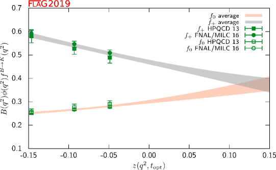
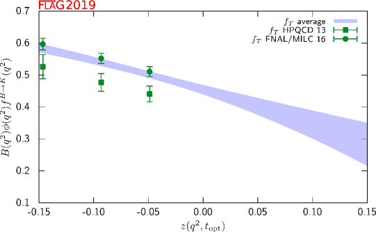
Figure 29: The $B\to K$ form factors $(1-q^{2}/m_{B^{*}}^{2})f_{+}(q^{2})$, $(1-q^{2}/m_{B^{*}(0+)}^{2})f_{0}(q^{2})$ and $(1-q^{2}/m_{B^{*}}^{2})f_{T}(q^{2})$ plotted versus $z$. (See text for a discussion of the data sets.) The grey, salmon and blue bands display our preferred $N^{+}=N^{0}=N^{T}=3$ BCL fit (eight parameters) to the plotted data with errors.

Lattice computations of form factors in channels with a vector meson in the final state face extra challenges with respect to the case of a pseudoscalar meson: the state is unstable, and the extraction of the relevant matrix element from correlation functions is significantly more complicated; $\chi$PT cannot be used as a guide to extrapolate results at unphysically heavy pion masses to the chiral limit. While field-theory procedures to take resonance effects into account are available [Luscher:1986pf, Luscher:1990ux, Luscher:1991cf, Lage:2009zv, Bernard:2010fp, Doring:2011vk, Hansen:2012tf, Briceno:2012yi, Dudek:2014qha], they have not yet been implemented in the existing preliminary computations, which therefore suffer from uncontrolled systematic errors in calculations of weak decay form factors into unstable vector meson final states, such as the $K^{*}$ or $\rho$ mesons.

As a consequence of the complexity of the problem, the level of maturity of these computations is significantly below the one present for pseudoscalar form factors. Therefore, we will only provide below a short guide to the existing results.

Concerning channels with vector mesons in the final state, Horgan et al. have obtained the seven form factors governing $B\to K^{*}\ell^{+}\ell^{-}$ (as well as those for $B_{s}\to\phi\,\ell^{+}\ell^{-}$) in Ref. [Horgan:2013hoa] using NRQCD $b$ quarks and asqtad staggered light quarks. In this work, they use a modified $z$-expansion to simultaneously extrapolate to the physical light-quark masses and continuum and extrapolate in $q^{2}$ to the full kinematic range. As discussed in Sec. 7.2, the modified $z$-expansion is not based on an underlying effective theory, and the associated uncertainties have yet to be fully studied. Horgan et al. use their form-factor results to calculate the differential branching fractions and angular distributions and discuss the implications for phenomenology in a companion paper [Horgan:2013pva]. Finally, preliminary results on $B\to K^{*}\ell^{+}\ell^{-}$ and $B_{s}\to\phi\ell^{+}\ell^{-}$ by RBC/UKQCD, have been reported in Refs. [Flynn:2015ynk, Flynn:2016vej, Lizarazo:2016myv].

8.4 Semileptonic form factors for $B_{(s)}\to D_{(s)}\ell\nu$ and $B\to D^{*}\ell\nu$

The semileptonic processes $B_{(s)}\rightarrow D_{(s)}\ell\nu$ and $B\rightarrow D^{*}\ell\nu$ have been studied extensively by experimentalists and theorists over the years. They allow for the determination of the CKM matrix element $|V_{cb}|$, an extremely important parameter of the Standard Model. The matrix elememt $V_{cb}$ appears in many quantities that serve as inputs to CKM unitarity triangle analyses and reducing its uncertainties is of paramount importance. For example, when $\epsilon_{K}$, the measure of indirect CP violation in the neutral kaon system, is written in terms of the parameters $\rho$ and $\eta$ that specify the apex of the unitarity triangle, a factor of $|V_{cb}|^{4}$ multiplies the dominant term. As a result, the errors coming from $|V_{cb}|$ (and not those from $B_{K}$) are now the dominant uncertainty in the Standard Model (SM) prediction for this quantity.

The decay rate for $B\rightarrow D\ell\nu$ can be parameterized in terms of vector and scalar form factors in the same way as, e.g., $B\to\pi\ell\nu$, see Sec. 8.3. The decay rate for $B\rightarrow D^{*}\ell\nu$ is different because the final-state hadron is spin-1. There are four form factors used to describe the vector and axial-vector current matrix elements that are needed to calculate this decay. We define the 4-velocity of the meson $P$ as $v_{P}=p_{P}/m_{P}$ and the polarization vector of the $D^{*}$ as $\epsilon$. When the light lepton $\ell=e$, or $\mu$, it is traditional to use $w=v_{B}\cdot v_{D^{(*)}}$ rather than $q^{2}$ as the variable upon which the form factors depend. Then, the form factors $h_{V}$, and $h_{A_{i}}$, with $i=1$, 2 or 3 are defined by

$$\langle D^{*}|V_{\mu}|B\rangle =\sqrt{m_{B}m_{D^{*}}}h_{V}(w)\varepsilon_{\mu\nu\alpha\beta}\epsilon^{*\nu}v_{D^{*}}^{\alpha}v_{B}^{\beta}\,,$$ (229)

$$\langle D^{*}|A_{\mu}|B\rangle =i\sqrt{m_{B}m_{D^{*}}}\left[h_{A_{1}}(w)(1+w)\epsilon^{*\mu}-h_{A_{2}}(w)\epsilon^{*}\cdot v_{B}{v_{B}}_{\mu}-h_{A_{3}}(w)\epsilon^{*}\cdot v_{B}{v_{D^{*}}}_{\mu}\right]\,.$$ (230)

The differential decay rates can then be written as

$$d\Gamma_{B^{-}\to D^{0}\ell^{-}\bar{\nu}}\over dw = \hbox{$G^{2}_{\rm F}m^{3}_{D}\over 48\pi^{3}$}(m_{B}+m_{D})^{2}(w^{2}-1)^{3/2}|\eta_{\mathrm{EW}}|^{2}|V_{cb}|^{2}|\mathcal{G}(w)|^{2},$$ (231)

$$d\Gamma_{B^{-}\to D^{0*}\ell^{-}\bar{\nu}}\over dw = \hbox{$G^{2}_{\rm F}m^{3}_{D^{*}}\over 4\pi^{3}$}(m_{B}-m_{D^{*}})^{2}(w^{2}-1)^{1/2}|\eta_{\mathrm{EW}}|^{2}|V_{cb}|^{2}\chi(w)|\mathcal{F}(w)|^{2},$$ (232)

where $w=v_{B}\cdot v_{D^{(*)}}$ (depending on whether the final-state meson is $D$ or $D^{*}$) and $\eta_{\mathrm{EW}}=1.0066$ is the 1-loop electroweak correction [Sirlin:1981ie]. The function $\chi(w)$ in Eq. (232) depends on the recoil $w$ and the meson masses, and reduces to unity at zero recoil [Antonelli:2009ws]. These formulas do not include terms that are proportional to the lepton mass squared, which can be neglected for $\ell=e,\mu$. Further details of the definitions of ${\cal F}$ and ${\cal G}$ may be found, e.g., in Ref. [Antonelli:2009ws]. Until recently, most unquenched lattice calculations for $B\rightarrow D^{*}\ell\nu$ and $B\rightarrow D\ell\nu$ decays focused on the form factors at zero recoil ${\cal F}^{B\rightarrow D^{*}}(1)$ and ${\cal G}^{B\rightarrow D}(1)$; these can then be combined with experimental input to extract $|V_{cb}|$. The main reasons for concentrating on the zero recoil point are that (i) the decay rate then depends on a single form factor, and (ii) for $B\rightarrow D^{*}\ell\nu$, there are no $\mathcal{O}(\Lambda_{QCD}/m_{Q})$ contributions due to Luke’s theorem [Luke:1990eg]. Further, the zero recoil form factor can be computed via a double ratio in which most of the current renormalization cancels and heavy-quark discretization errors are suppressed by an additional power of $\Lambda_{QCD}/m_{Q}$. Recent work on $B\rightarrow D^{(*)}\ell\nu$ transitions has started to explore the dependence of the relevant form factors on the momentum transfer, using a similar methodology to the one employed in $B\to\pi\ell\nu$ transitions; we refer the reader to Sec. 8.3 for a detailed discussion.

Early computations of the form factors for $B\rightarrow D\ell\nu$ decays include $N_{f}=2+1$ results by FNAL/MILC [Okamoto:2004xg, Qiu:2013ofa] for ${\cal G}^{B\rightarrow D}(1)$ and the $N_{f}=2$ study by Atoui et al. [Atoui:2013zza], that in addition to providing ${\cal G}^{B\rightarrow D}(1)$ explored the $w>1$ region. This latter work also provided the first results for $B_{s}\rightarrow D_{s}\ell\nu$ amplitudes, again including information about the momentum-transfer dependence; this will allow for an independent determination of $|V_{cb}|$ as soon as experimental data is available for these transitions. The first published unquenched results for ${\cal F}^{B\rightarrow D^{*}}(1)$, obtained by FNAL/MILC, date from 2008 [Bernard:2008dn]. In 2014 and 2015, significant progress was achieved in $N_{f}=2+1$ computations: the FNAL/MILC value for ${\cal F}^{B\rightarrow D^{*}}(1)$ was updated in Ref. [Bailey:2014tva], and full results for $B\rightarrow D\ell\nu$ at $w\geq 1$ were published by FNAL/MILC [Lattice:2015rga] and HPQCD [Na:2015kha]. These works also provided full results for the scalar form factor, allowing analysis of the decay with a final-state $\tau$. Since the previous version of this review, there are new results for $B_{s}\rightarrow D_{s}\ell\nu$ form factors over the full kinematic range for $N_{f}=2+1$ from HPQCD [Monahan:2016qxu, Monahan:2017uby], and for ${{B}_{(s)}\to D_{(s)}^{*}\ell{\nu}}$ form factors at zero recoil with $N_{f}=2+1+1$ also from HPQCD [Harrison:2016gup, Harrison:2017fmw]. There has also been significant progress on heavy-baryon decay. Reference [Datta:2017aue] calculates the tensor form factors for decay ${\Lambda}_{b}\to{\Lambda}_{c}\tau{\overline{\nu}}_{\tau}$ and considers the phenomenological implications.

In the discussion below, we mainly concentrate on the latest generation of results, which supersedes previous $N_{f}=2+1$ determinations and allows for an extraction of $|V_{cb}|$ that incorporates information about the $q^{2}$-dependence of the decay rate (cf. Sec. LABEL:sec:Vcb).

8.4.1 $B_{(s)}\rightarrow D_{(s)}$ decays

We will first discuss the $N_{f}=2+1$ computations of $B\rightarrow D\ell\nu$ by FNAL/MILC and HPQCD mentioned above, both based on MILC asqtad ensembles. Full details about all the computations are provided in Tab. 1 and in the tables in Appendix LABEL:app:BtoD_Notes.

The FNAL/MILC study [Lattice:2015rga] employs ensembles at four values of the lattice spacing ranging between approximately $0.045~{}{\rm fm}$ and $0.12~{}{\rm fm}$, and several values of the light-quark mass corresponding to pions with RMS masses ranging between $260~{}{\rm MeV}$ and $670~{}{\rm MeV}$ (with just one ensemble with $M_{\pi}^{\rm RMS}\simeq 330~{}{\rm MeV}$ at the finest lattice spacing). The $b$ and $c$ quarks are treated using the Fermilab approach. The quantities directly studied are the form factors $h_{\pm}$ defined by

$$\hbox{$\langle D(p_{D})|i\bar{c}\gamma_{\mu}b|B(p_{B})\rangle\over\sqrt{m_{D}m_{B}}$}=h_{+}(w)(v_{B}+v_{D})_{\mu}\,+\,h_{-}(w)(v_{B}-v_{D})_{\mu}\,,$$ (233)

which are related to the standard vector and scalar form factors by

$$f_{+}(q^{2}) =\hbox{$1\over 2\sqrt{r}$}\,\left[(1+r)h_{+}(w)-(1-r)h_{-}(w)\right]\,,$$ (234)

$$f_{0}(q^{2}) =\sqrt{r}\left[\hbox{$1+w\over 1+r$}\,h_{+}(w)\,+\,\hbox{$1-w\over 1-r$}\,h_{-}(w)\right]\,,$$ (235)

with $r=m_{D}/m_{B}$. (Recall that $q^{2}=(p_{B}-p_{D})^{2}=m_{B}^{2}+m_{D}^{2}-2wm_{B}m_{D}$.) The hadronic form factor relevant for experiment, $\mathcal{G}(w)$, is then obtained from the relation $\mathcal{G}(w)=4rf_{+}(q^{2})/(1+r)$. The form factors are obtained from double ratios of three-point functions in which the flavour-conserving current renormalization factors cancel. The remaining matching factor $\rho_{V^{\mu}_{cb}}$ is estimated with 1-loop lattice perturbation theory. In order to obtain $h_{\pm}(w)$, a joint continuum-chiral fit is performed to an ansatz that contains the light-quark mass and lattice-spacing dependence predicted by next-to-leading order HMrS$\chi$PT, and the leading dependence on $m_{c}$ predicted by the heavy-quark expansion ($1/m_{c}^{2}$ for $h_{+}$ and $1/m_{c}$ for $h_{-}$). The $w$-dependence, which allows for an interpolation in $w$, is given by analytic terms up to $(1-w)^{2}$, as well as a contribution from the logarithm proportional to $g^{2}_{D^{*}D\pi}$. The total resulting systematic error is $1.2\%$ for $f_{+}$ and $1.1\%$ for $f_{0}$. This dominates the final error budget for the form factors. After $f_{+}$ and $f_{0}$ have been determined as functions of $w$ within the interval of values of $q^{2}$ covered by the computation, synthetic data points are generated to be subsequently fitted to a $z$-expansion of the BGL form, cf. Sec. 8.3, with pole factors set to unity. This in turn enables one to determine $|V_{cb}|$ from a joint fit of this $z$-expansion and experimental data. The value of the zero-recoil form factor resulting from the $z$-expansion is

$${\cal G}^{B\rightarrow D}(1)=1.054(4)_{\rm stat}(8)_{\rm sys}\,.$$ (236)

The HPQCD computations [Na:2015kha, Monahan:2017uby] use ensembles at two values of the lattice spacing, $a=0.09,~{}0.12~{}{\rm fm}$, and two and three values of light-quark masses, respectively. The $b$ quark is treated using NRQCD, while for the $c$ quark the HISQ action is used. The form factors studied, extracted from suitable three-point functions, are

$$\langle D_{(s)}(p_{D_{(s)}})|V^{0}|B_{(s)}\rangle=\sqrt{2M_{B_{(s)}}}f^{(s)}_{\parallel}\,,~{}~{}~{}~{}~{}~{}~{}~{}\langle D_{(s)}(p_{D_{(s)}})|V^{k}|B_{(s)}\rangle=\sqrt{2M_{B_{(s)}}}p^{k}_{D_{(s)}}f^{(s)}_{\perp}\,,$$ (237)

where $V_{\mu}$ is the relevant vector current and the $B_{(s)}$ rest frame is assumed. The standard vector and scalar form factors are retrieved as

$$f^{(s)}_{+} =\hbox{$1\over\sqrt{2M_{B_{(s)}}}$}f^{(s)}_{\parallel}\,+\,\hbox{$1\over\sqrt{2M_{B_{(s)}}}$}(M_{B_{(s)}}-E_{D_{(s)}})f^{(s)}_{\perp}\,,$$ (238)

$$f^{(s)}_{0} =\hbox{$\sqrt{2M_{B_{(s)}}}\over M_{B_{(s)}}^{2}-M_{D_{(s)}}^{2}$}\left[(M_{B_{(s)}}-E_{D_{(s)}})f^{(s)}_{\parallel}+(M_{B_{(s)}}^{2}-E_{D_{(s)}}^{2})f^{(s)}_{\perp}\right]\,.$$ (239)

The currents in the effective theory are matched at 1-loop to their continuum counterparts. Results for the form factors are then fitted to a modified BCL $z$-expansion ansatz, that takes into account simultaneously the lattice spacing, light-quark masses, and $q^{2}$-dependence. For the mass dependence NLO chiral logarithms are included, in the form obtained in hard-pion $\chi$PT. As in the case of the FNAL/MILC computation, once $f_{+}$ and $f_{0}$ have been determined as functions of $q^{2}$, $|V_{cb}|$ can be determined from a joint fit of this $z$-expansion and experimental data. The works quote for the zero-recoil vector form factor the result

$${\cal G}^{B\rightarrow D}(1)=1.035(40)\,~{}~{}~{}~{}{\cal G}^{B_{s}\rightarrow D_{s}}(1)=1.068(4)\,.$$ (240)

The HPQCD and FNAL/MILC results for $B\to D$ differ by less than half a standard deviation (assuming they are uncorrelated, which they are not as some of the ensembles are common) primarily because of lower precision of the former result. The HPQCD central value is smaller by 1.8 of the FNAL/MILC standard deviations than the FNAL/MILC value. The dominant source of errors in the $|V_{cb}|$ determination by HPQCD are discretization effects and the systematic uncertainty associated with the perturbative matching.

In order to combine the form factors determinations of HPQCD and FNAL/MILC into a lattice average, we proceed in a similar way as with $B\to\pi\ell\nu$ and $B_{s}\to K\ell\nu$ above. FNAL/MILC quotes synthetic values for the form factors at three values of $w$ (or, alternatively, $q^{2}$) with a full correlation matrix, which we take directly as input. In the case of HPQCD, we use their preferred modified $z$-expansion parameterization to produce synthetic values of the form factors at two different values of $q^{2}$. This leaves us with a total of five data points in the kinematical range $w\in[1.00,1.11]$. As in the case of $B\to\pi\ell\nu$, we conservatively assume a 100% correlation of statistical uncertainties between HPQCD and FNAL/MILC. We then fit this data set to a BCL ansatz, using $t_{+}=(M_{B^{0}}+M_{D^{\pm}})^{2}\simeq 51.12~{}\,\mathrm{GeV}^{2}$ and $t_{0}=(M_{B^{0}}+M_{D^{\pm}})(\sqrt{M_{B^{0}}}-\sqrt{M_{D^{\pm}}})^{2}\simeq 6.19~{}\,\mathrm{GeV}^{2}$. In our fits, pole factors have been set to unity—i.e., we do not take into account the effect of sub-threshold poles, which is then implicitly absorbed into the series coefficients. The reason for this is our imperfect knowledge of the relevant resonance spectrum in this channel, which does not allow us to decide the precise number of poles needed. This in turn implies that unitarity bounds do not rigorously apply, which has to be taken into account when interpreting the results (cf. Appendix LABEL:sec:zparam).

With a procedure similar to what we adopted for the $B\to\pi$ and $B_{s}\to K$ cases, we impose the kinematic constraint at $q^{2}=0$ by expressing the $a^{0}_{N^{0}-1}$ coefficient in the $z$-expansion of $f_{0}$ in terms of all other coefficients. As mentioned above, FNAL/MILC provides synthetic data for $f_{+}$ and $f_{0}$ including correlations; HPQCD presents the result of simultaneous $z$-fits to the two form factors including all correlations, thus enabling us to generate a complete set of synthetic data for $f_{+}$ and $f_{0}$. Since both calculations are based on MILC ensembles, we then reconstruct the off-diagonal HPQCD-FNAL/MILC entries of the covariance matrix by conservatively assuming that statistical uncertainties are 100% correlated. The Fermilab/MILC (HPQCD) statistical error is 58% (31%) of the total error for every $f_{+}$ value, and 64% (49%) for every $f_{0}$ one. Using this information we can easily build the off-diagonal block of the overall covariance matrix (e.g., the covariance between $[f_{+}(q_{1}^{2})]_{\rm FNAL}$ and $[f_{0}(q_{2}^{2})]_{\rm HPQCD}$ is $(\delta[f_{+}(q_{1}^{2})]_{\rm FNAL}\times 0.58)\;(\delta[f_{0}(q_{2}^{2})]_{\rm HPQCD}\times 0.49)$, where $\delta f$ is the total error).

For our central value, we choose an $N^{+}=N^{0}=3$ BCL fit, shown in Tab. 47. The coefficient $a_{3}^{+}$ can be obtained from the values for $a_{0}^{+}$–$a_{2}^{+}$ using Eq. (LABEL:eq:red_coeff). The fit is illustrated in Fig. 30.

$B\to D\;(N_{f}=2+1)$
$a_{n}^{i}$	Central Values	Correlation Matrix
$a_{0}^{+}$	0.909 (14)	1	0.737	0.594	0.976	0.777
$a_{1}^{+}$	$-$7.11 (65)	0.737	1	0.940	0.797	0.992
$a_{2}^{+}$	66 (11)	0.594	0.940	1	0.666	0.938
$a_{0}^{0}$	0.794 (12)	0.976	0.797	0.666	1	0.818
$a_{1}^{0}$	$-$2.45 (65)	$-$ 0.777	0.992	0.938	0.818	1

Table 47: Coefficients and correlation matrix for the $N^{+}=N^{0}=3$ $z$-expansion of the $B\to D$ form factors $f_{+}$ and $f_{0}$.

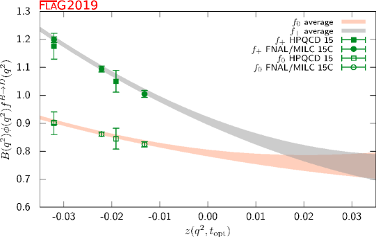
Figure 30: The form factors $f_{+}(q^{2})$ and $f_{0}(q^{2})$ for $B\to D\ell\nu$ plotted versus $z$. (See text for a discussion of the data sets.) The grey and salmon bands display our preferred $N^{+}=N^{0}=3$ BCL fit (five parameters) to the plotted data with errors.

Reference [Atoui:2013zza] is the only existing $N_{f}=2$ work on $B\rightarrow D\ell\nu$ transitions, that furthermore provided the first available results for $B_{s}\rightarrow D_{s}\ell\nu$. This computation uses the publicly available ETM configurations obtained with the twisted-mass QCD action at maximal twist. Four values of the lattice spacing, ranging between $0.054~{}{\rm fm}$ and $0.098~{}{\rm fm}$, are considered, with physical box lengths ranging between $1.7~{}{\rm fm}$ and $2.7~{}{\rm fm}$. At two values of the lattice spacing two different physical volumes are available. Charged-pion masses range between $\approx 270~{}{\rm MeV}$ and $\approx 490~{}{\rm MeV}$, with two or three masses available per lattice spacing and volume, save for the $a\approx 0.054~{}{\rm fm}$ point at which only one light mass is available for each of the two volumes. The strange- and heavy-valence quarks are also treated with maximally twisted-mass QCD.

The quantities of interest are again the form factors $h_{\pm}$ defined above. In order to control discretization effects from the heavy quarks, a strategy similar to the one employed by the ETM collaboration in their studies of $B$-meson decay constants (cf. Sec. 8.1) is employed: the value of ${\cal G}(w)$ is computed at a fixed value of $m_{c}$ and several values of a heavier quark mass $m_{h}^{(k)}=\lambda^{k}m_{c}$, where $\lambda$ is a fixed scaling parameter, and step-scaling functions are built as

$$\Sigma_{k}(w)=\hbox{${\cal G}(w,\lambda^{k+1}m_{c},m_{c},a^{2})\over{\cal G}(w,\lambda^{k}m_{c},m_{c},a^{2})$}\,.$$ (241)

Each ratio is extrapolated to the continuum limit, $\sigma_{k}(w)=\lim_{a\to 0}\Sigma_{k}(w)$. One then exploits the fact that the $m_{h}\to\infty$ limit of the step-scaling is fixed—in particular, it is easy to find from the heavy-quark expansion that $\lim_{m_{h}\to\infty}\sigma(1)=1$. In this way, the physical result at the $b$-quark mass can be reached by interpolating $\sigma(w)$ between the charm region (where the computation can be carried out with controlled systematics) and the known static limit value.

In practice, the values of $m_{c}$ and $m_{s}$ are fixed at each value of the lattice spacing such that the experimental kaon and $D_{s}$ masses are reached at the physical point, as determined in Ref. [Blossier:2010cr]. For the scaling parameter, $\lambda=1.176$ is chosen, and eight scaling steps are performed, reaching $m_{h}/m_{c}=1.176^{9}\simeq 4.30$, approximately corresponding to the ratio of the physical $b$- and $c$-masses in the $\overline{\rm MS}$ scheme at $2~{}{\rm GeV}$. All observables are obtained from ratios that do not require (re)normalization. The ansatz for the continuum and chiral extrapolation of $\Sigma_{k}$ contains a constant and linear terms in $m_{\rm sea}$ and $a^{2}$. Twisted boundary conditions in space are used for valence-quark fields for better momentum resolution. Applying this strategy the form factors are finally obtained at four reference values of $w$ between $1.004$ and $1.062$, and, after a slight extrapolation to $w=1$, the result is quoted

$${\cal G}^{B_{s}\rightarrow D_{s}}(1)=1.052(46)\,.$$ (242)

The authors also provide values for the form factor relevant for the meson states with light-valence quarks, obtained from a similar analysis to the one described above for the $B_{s}\rightarrow D_{s}$ case. Values are quoted from fits with and without a linear $m_{\rm sea}/m_{s}$ term in the chiral extrapolation. The result in the former case, which safely covers systematic uncertainties, is

$${\cal G}^{B\rightarrow D}(1)=1.033(95)\,.$$ (243)

Given the identical strategy, and the small sensitivity of the ratios used in their method to the light valence- and sea-quark masses, we assign this result the same ratings in Tab. 1 as those for their calculation of ${\cal G}^{B_{s}\rightarrow D_{s}}(1)$. Currently the precision of this calculation is not competitive with that of $N_{f}=2+1$ works, but this is due largely to the small number of configurations analysed by Atoui et al. The viability of their method has been clearly demonstrated, however, which leaves significant room for improvement on the errors of both the $B\to D$ and $B_{s}\to D_{s}$ form factors with this approach by including either additional two-flavour data or analysing more recent ensembles with $N_{f}>2$.

Finally, Atoui et al. also study the scalar and tensor form factors, as well as the momentum-transfer dependence of $f_{+,0}$. The value of the ratio $f_{0}(q^{2})/f_{+}(q^{2})$ is provided at a reference value of $q^{2}$ as a proxy for the slope of ${\cal G}(w)$ around the zero-recoil limit.

8.4.2 Ratios of $B\to D\ell\nu$ form factors

The availability of results for the scalar form factor $f_{0}$ for $B\to D\ell\nu$ amplitudes allows us to study interesting observables that involve the decay in the $\tau$ channel. One such quantity is the ratio

$$R(D)={\cal B}(B\rightarrow D\tau\nu)/{\cal B}(B\rightarrow D\ell\nu)\hskip 28.45274pt\mbox{with}\;\ell=e,\mu\,,$$ (244)

which is sensitive to $f_{0}$, and can be accurately determined by experiment. Indeed, the recent availability of experimental results for $R(D)$ has made this quantity particularly relevant in the search for possible physics beyond the Standard Model. Both FNAL/MILC and HPQCD provide values for $R(D)$ from their recent form factor computations, discussed above. The quoted values by FNAL/MILC and HPQCD are

$$R(D)=0.299(11)\,\ref{~}\mbox{~{}\cite[cite]{[\@@bibref{Number}{Lattice:2015rga}{}{}]}}\,,~{}~{}~{}~{}~{}R(D)=0.300(8)\,\ref{~}\mbox{~{}\cite[cite]{[\@@bibref{Number}{Na:2015kha}{}{}]}}\,.$$ (245)

These results are in excellent agreement, and can be averaged (using the same considerations for the correlation between the two computations as we did in the averaging of form factors) into

$$R(D)=0.300(8)\,,~{}~{}~{}~{}\mbox{our average.}$$ (246)

This result is about $2.3\sigma$ lower than the current experimental average for this quantity. It has to be stressed that achieving this level of precision critically depends on the reliability with which the low-$q^{2}$ region is controlled by the parameterizations of the form factors. It is also worth mentioning that if experimental data for $B\to D\ell\nu$ are used to further constrain $R(D)$ as part of a global fit, it is possible to decrease the error substantially, cf. the value $R(D)=0.299(3)$ quoted in [Bigi:2016mdz].

HPQCD also computes a new value for $R(D_{s})$, the analog of $R(D)$, with both heavy-light mesons containing a strange quark [Monahan:2017uby]:

$$R(D_{s})=0.301(6)\,.$$ (247)

Another area of immediate interest in searches for physics beyond the Standard Model is the measurement of $B_{s}\rightarrow\mu^{+}\mu^{-}$ decays, recently studied at the LHC. In addition to the $B_{s}$ decay constant (see Sec. 8.1), one of the hadronic inputs required by the LHCb analysis is the ratio of $B_{q}$ meson ($q=d,s$) fragmentation fractions $f_{s}/f_{d}$. A dedicated $N_{f}=2+1$ study by FNAL/MILC [Bailey:2012rr] addresses the ratios of scalar form factors $f_{0}^{(q)}(q^{2})$, and quotes:

$$f_{0}^{(s)}(M_{\pi}^{2})/f_{0}^{(d)}(M_{K}^{2})=1.046(44)(15),\qquad f_{0}^{(s)}(M_{\pi}^{2})/f_{0}^{(d)}(M_{\pi}^{2})=1.054(47)(17),$$ (248)

where the first error is statistical and the second systematic. The more recent results from HPQCD [Monahan:2017uby] are:

$$f_{0}^{(s)}(M_{\pi}^{2})/f_{0}^{(d)}(M_{K}^{2})=1.000(62),\qquad f_{0}^{(s)}(M_{\pi}^{2})/f_{0}^{(d)}(M_{\pi}^{2})=1.006(62).$$ (249)

Results from both groups lead to fragmentation fraction ratios $f_{s}/f_{d}$ that are consistent with LHCb’s measurements via other methods [Aaij:2011hi].

8.4.3 $B\rightarrow D^{*}$ decays

The most precise computation of the zero-recoil form factors needed for the determination of $|V_{cb}|$ from exclusive $B$ semileptonic decays comes from the $B\rightarrow D^{*}\ell\nu$ form factor at zero recoil ${\cal F}^{B\rightarrow D^{*}}(1)$, calculated by the FNAL/MILC collaboration. The original computation, published in Ref. [Bernard:2008dn], has now been updated [Bailey:2014tva] by employing a much more extensive set of gauge ensembles and increasing the statistics of the ensembles originally considered, while preserving the analysis strategy. There is currently no unquenched computation of the relevant form factors at nonzero recoil.

This work uses the MILC $N_{f}=2+1$ ensembles. The bottom and charm quarks are simulated using the clover action with the Fermilab interpretation and light quarks are treated via the asqtad staggered fermion action. Recalling the definition of the form factors in Eq. (230), at zero recoil ${\cal F}^{B\rightarrow D^{*}}(1)$ reduces to a single form factor $h_{A_{1}}(1)$ coming from the axial-vector current

$$\langle D^{*}(v,\epsilon^{\prime})|{\cal A}_{\mu}|\overline{B}(v)\rangle=i\sqrt{2m_{B}2m_{D^{*}}}\;{\epsilon^{\prime}_{\mu}}^{\ast}h_{A_{1}}(1),$$ (250)

where $\epsilon^{\prime}$ is the polarization of the $D^{*}$. The form factor is accessed through a ratio of three-point correlators, viz.,

$${\cal R}_{A_{1}}=\hbox{$\langle D^{*}|\bar{c}\gamma_{j}\gamma_{5}b|\overline{B}\rangle\;\langle\overline{B}|\bar{b}\gamma_{j}\gamma_{5}c|D^{*}\rangle\over\langle D^{*}|\bar{c}\gamma_{4}c|D^{*}\rangle\;\langle\overline{B}|\bar{b}\gamma_{4}b|\overline{B}\rangle$}=|h_{A_{1}}(1)|^{2}.$$ (251)

Simulation data is obtained on MILC ensembles with five lattice spacings, ranging from $a\approx 0.15~{}{\rm fm}$ to $a\approx 0.045~{}{\rm fm}$, and as many as five values of the light-quark masses per ensemble (though just one at the finest lattice spacing). Results are then extrapolated to the physical, continuum/chiral, limit employing staggered $\chi$PT.

The $D^{*}$ meson is not a stable particle in QCD and decays predominantly into a $D$ plus a pion. Nevertheless, heavy-light meson $\chi$PT can be applied to extrapolate lattice simulation results for the $B\to D^{*}\ell\nu$ form factor to the physical light-quark mass. The $D^{*}$ width is quite narrow, 0.096 MeV for the $D^{*\pm}(2010)$ and less than 2.1 MeV for the $D^{*0}(2007)$, making this system much more stable and long lived than the $\rho$ or the $K^{*}$ systems. The fact that the $D^{*}-D$ mass difference is close to the pion mass leads to the well-known “cusp” in ${\cal R}_{A_{1}}$ just above the physical pion mass [Randall:1993qg, Savage:2001jw, Hashimoto:2001nb]. This cusp makes the chiral extrapolation sensitive to values used in the $\chi$PT formulas for the $D^{*}D\pi$ coupling $g_{D^{*}D\pi}$. The error budget in Ref. [Bailey:2014tva] includes a separate error of 0.3% coming from the uncertainty in $g_{D^{*}D\pi}$ in addition to general chiral extrapolation errors in order to take this sensitivity into account.

The final updated value presented in Ref. [Bailey:2014tva] is

$$N_{f}=2+1:\;\;{\cal F}^{B\rightarrow D^{*}}(1)=0.906(4)(12)\,,$$ (252)

where the first error is statistical, and the second the sum of systematic errors added in quadrature, making up a total error of $1.4$% (down from the original $2.6$% of Ref. [Bernard:2008dn]). The largest systematic uncertainty comes from discretization errors followed by effects of higher-order corrections in the chiral perturbation theory ansatz.

Since the previous version of this review, the HPQCD collaboration has published the first study of ${{B}_{(s)}\to D_{(s)}^{*}\ell{\nu}}$ form factors at zero recoil for $N_{f}=2+1+1$ using eight MILC ensembles with lattice spacing $a\approx 0.15$, 0.12, and 0.09 [Monahan:2017uby]. There are three ensembles with varying light-quark masses for the two coarser lattice spacings and two choices of light-quark mass for the finest lattice spacing. In each case, there is one ensemble for which the light-quark mass is very close to the physical value. The $b$ quark is treated using NRQCD and the light quarks are treated using the HISQ action. The resulting zero-recoil form factors are:

$$N_{f}=2+1+1:\;\;{\mathcal{F}}^{B\rightarrow D^{*}}(1)=0.895(10)(24)\,,~{}~{}~{}~{}{\mathcal{F}}^{B_{s}\to D_{s}^{*}}(1)=0.883(12)(28)\,.$$ (253)

At Lattice 2018, two groups presented preliminary results for the $B\to D^{*}\ell\nu$ semileptonic decay. From JLQCD, there was a poster describing their calculations for zero and nonzero recoil using $N_{f}=2+1$ Möbius domain-wall ensembles. Two lattice spacings of roughly 0.079 and 0.055 fm were used with bottom-quark mass limited to 2.4 times the charm-quark mass to control the heavy-quark discretization effects. In addition, JLQCD is studying $B\to D\ell\nu$. From FNAL/MILC there was a presentation of preliminary results using 15 $N_{f}=2+1$ asqtad sea-quark ensembles with lattice spacing between approximately 0.15 and 0.045 fm. The heavy quarks are treated using the clover action with the Fermilab interpretation. In addition, HPQCD presented preliminary results for $B_{s}\to D_{s}^{(*)}\ell\nu$ using HISQ quarks for all valence and sea quarks. The calculation uses three of MILC’s $N_{f}=2+1+1$ HISQ ensembles with $a\approx 0.09$, 0.06 and 0.045 fm. An advantage of the all-HISQ approach is that there is no need for perturbative renormalization of the axial-vector- or vector-current.

Collaboration	Ref.	$N_{f}$	publication status	continuum extrapolation	chiral extrapolation	finite volume	renormalization	heavy-quark treatment	$w=1$ form factor / ratio
Atoui 13	[Atoui:2013zza]	2	A	$\bigstar$	$\circ$	$\bigstar$	—	✓	${\mathcal{G}}^{B\to D}(1)$	1.033(95)
HPQCD 15, HPQCD 17	[Na:2015kha, Monahan:2017uby]	2+1	A	$\circ$	$\circ$	$\circ$	$\circ$	✓	${\mathcal{G}}^{B\to D}(1)$	1.035(40)
FNAL/MILC 15C	[Lattice:2015rga]	2+1	A	$\bigstar$	$\circ$	$\bigstar$	$\circ$	✓	${\mathcal{G}}^{B\to D}(1)$	$1.054(4)(8)$
Atoui 13	[Atoui:2013zza]	2	A	$\bigstar$	$\circ$	$\bigstar$	—	✓	${\mathcal{G}}^{B_{s}\to D_{s}}(1)$	1.052(46)
HPQCD 15, HPQCD 17	[Na:2015kha, Monahan:2017uby]	2+1	A	$\circ$	$\circ$	$\circ$	$\circ$	✓	${\mathcal{G}}^{B_{s}\to D_{s}}(1)$	1.068(40)
FNAL/MILC 14	[Bailey:2014tva]	2+1	A	$\bigstar$	$\circ$	$\bigstar$	$\circ$	✓	${\mathcal{F}}^{B\to D^{*}}(1)$	0.906(4)(12)
HPQCD 17B	[Harrison:2017fmw]	2+1+1	A	$\circ$	$\bigstar$	$\bigstar$	$\circ$	✓	${\mathcal{F}}^{B\to D^{*}}(1)$	0.895(10)(24)
HPQCD 17B	[Harrison:2017fmw]	2+1+1	A	$\circ$	$\bigstar$	$\bigstar$	$\circ$	✓	${\mathcal{F}}^{B_{s}\to D_{s}^{*}}(1)$	0.883(12)(28)
FNAL/MILC 15C	[Lattice:2015rga]	2+1	A	$\bigstar$	$\circ$	$\bigstar$	$\circ$	✓	$R(D)$	0.299(11)
HPQCD 15, HPQCD 17	[Na:2015kha, Monahan:2017uby]	2+1	A	$\circ$	$\circ$	$\circ$	$\circ$	✓	$R(D)$	0.300(8)

Table 48: Lattice results for the $B_{(s)}\to D_{(s)}^{(*)}\ell\nu$ semileptonic form factors and $R(D_{(s)})$.

8.5 Semileptonic form factors for $B_{c}\to\eta_{c}\ell\nu$ and $B_{c}\to J/\psi\ell\nu$

In 2016, preliminary results for the decays $B_{c}\to\eta_{c}\ell\nu$ and $B_{c}\to J/\psi\ell\nu$ were presented at two conferences by the HPQCD collaboration [Lytle:2016ixw, Colquhoun:2016osw]. The calculations use both NRQCD and HISQ actions for the valence $b$ quark, and the HISQ action for the $c$ quark (both valence and sea). The calculations were done using five ensembles from the MILC collaboration with $N_{f}=2+1+1$ and lattice spacings between approximately 0.15 and 0.045 fm. Only ensembles with $m_{l}/m_{s}=0.2$ are used although ones with a physical light-quark mass are available. For the HISQ formalism, a range of heavy-quark masses obeying $am_{h}<0.8$ is used and an extrapolation $m_{h}\to m_{b}$ is made. Comparison of results using NRQCD and HISQ allows an improved normalization for the NRQCD currents as the HISQ currents do not require renormalization.

8.6 Semileptonic form factors for $\Lambda_{b}\to p\ell\nu$ and $\Lambda_{b}\to\Lambda_{c}\ell\nu$

Lattice-QCD computations for heavy-quark physics has been extended to the study of semileptonic decays of the $\Lambda_{b}$ baryon, with first unquenched results away from the static limit provided in a work by Detmold, Lehner, and Meinel [Detmold:2015aaa]. The importance of this result is that, together with a recent analysis by LHCb of the ratio of decay rates $\Gamma(\Lambda_{b}\to p\ell\nu)/\Gamma(\Lambda_{b}\to\Lambda_{c}\ell\nu)$ [Aaij:2015bfa], it allows for an exclusive determination of the ratio $|V_{ub}|/|V_{cb}|$ largely independent from the outcome of different exclusive channels, thus contributing a very interesting piece of information to the existing tensions in the determination of third-column CKM matrix elements (cf. Secs. 8.7, and LABEL:sec:Vcb).

The amplitudes of the decays $\Lambda_{b}\to p\ell\nu$ and $\Lambda_{b}\to\Lambda_{c}\ell\nu$ receive contributions from both the vector and the axial components of the current in the matrix elements $\langle p|\bar{q}\gamma^{\mu}(\mathbf{1}-\gamma_{5})b|\Lambda_{b}\rangle$ and $\langle\Lambda_{c}|\bar{q}\gamma^{\mu}(\mathbf{1}-\gamma_{5})b|\Lambda_{b}\rangle$, and can be parameterized in terms of six different form factors—see, e.g., Ref. [Feldmann:2011xf] for a complete description. They split into three form factors $f_{+}$, $f_{0}$, $f_{\perp}$ in the parity-even sector, mediated by the vector component of the current, and another three form factors $g_{+},g_{0},g_{\perp}$ in the parity-odd sector, mediated by the axial component. All of them provide contributions that are parametrically comparable.

The computation of Detmold et al. uses RBC/UKQCD $N_{f}=2+1$ DWF ensembles, and treats the $b$ and $c$ quarks within the Columbia RHQ approach. Two values of the lattice spacing ($a\sim 0.112,~{}0.085~{}{\rm fm}$) are considered, with the absolute scale set from the $\Upsilon(2S)$–$\Upsilon(1S)$ splitting. Sea pion masses lie in a narrow interval ranging from slightly above $400~{}{\rm MeV}$ to slightly below $300~{}{\rm MeV}$, keeping $m_{\pi}L\gtrsim 4$; however, lighter pion masses are considered in the valence DWF action for the $u,d$ quarks, leading to partial quenching effects in the chiral extrapolation. More importantly, this also leads to values of $M_{\pi,{\rm min}}L$ close to $3.0$ (cf. Appendix LABEL:app:BtoPi_Notes for details); compounded with the fact that there is only one lattice volume in the computation, an application of the FLAG criteria would lead to a $\blacksquare$ rating for finite-volume effects. It has to be stressed, however, that our criteria have been developed in the context of meson physics, and their application to the baryon sector is not straightforward; as a consequence, we will refrain from providing a conclusive rating of this computation for the time being.

Results for the form factors are obtained from suitable three-point functions, and fitted to a modified $z$-expansion ansatz that combines the $q^{2}$-dependence with the chiral and continuum extrapolations. The main results of the paper are the predictions (errors are statistical and systematic, respectively)

$$\zeta_{p\mu\bar{\nu}}(15{\rm GeV}^{2}) \equiv\hbox{$1\over|V_{ub}|^{2}$}\int_{15~{}{\rm GeV}^{2}}^{q^{2}_{\rm max}}\hbox{${\rm d}\Gamma(\Lambda_{b}\to p\mu^{-}\bar{\nu}_{\mu})\over{\rm d}q^{2}$}\,{\rm d}q^{2} =12.31(76)(77)~{}{\rm ps}^{-1}\,,$$ (254)

$$\zeta_{\Lambda_{c}\mu\bar{\nu}}(7{\rm GeV}^{2}) \equiv\hbox{$1\over|V_{cb}|^{2}$}\int_{7~{}{\rm GeV}^{2}}^{q^{2}_{\rm max}}\hbox{${\rm d}\Gamma(\Lambda_{b}\to\Lambda_{c}\mu^{-}\bar{\nu}_{\mu})\over{\rm d}q^{2}$}\,{\rm d}q^{2} =8.37(16)(34)~{}{\rm ps}^{-1}\,,$$ (255)

$$\zeta_{p\mu\bar{\nu}}(15{\rm GeV}^{2})\over\zeta_{\Lambda_{c}\mu\bar{\nu}}(7{\rm GeV}^{2}) =1.471(95)(109)\,,$$ (256)

which are the input for the LHCb analysis. Predictions for the total rates in all possible lepton channels, as well as for ratios similar to $R(D)$ (cf. Sec. 8.4) between the $\tau$ and light-lepton channels are also available.

Since the previous version of this review, there have been three papers [Detmold:2016pkz, Meinel:2016cxo, Datta:2017aue] extending study of the $\Lambda_{b}$ and two [Meinel:2016dqj, Meinel:2017ggx] studying the $\Lambda_{c}$. Reference [Detmold:2016pkz] studies the rare decay $\Lambda_{b}\to\Lambda\ell^{+}\ell^{-}$. The lattice setup is identical, and similar considerations as above thus apply. Furthermore, the renormalization of the tensor current is carried out adopting a mostly nonperturbative renormalization strategy, without however computing the residual renormalization factor $\rho_{T^{\mu\nu}}$, which is set to its tree-level value. While the matching systematic uncertainty is augmented to take this fact into account, the procedure implies that the current retains an uncanceled logarithmic divergence at $\mathcal{O}(\alpha_{s})$.

Reference [Meinel:2016cxo] is an exploratory study of the decay $\Lambda_{b}\to\Lambda(1520)\ell^{+}\ell^{-}$ using a single gauge ensemble presented at Lattice 2016. Reference [Datta:2017aue] includes new results for ${\Lambda}_{b}\to{\Lambda}_{c}$ for the tensor form factors. The main focus of this paper is the phenomenology of the ${\Lambda}_{b}\to{\Lambda}_{c}\tau{\overline{\nu}}_{\tau}$ decay and how it can be used to limit contributions from beyond the standard model physics.

8.7 Determination of $|V_{ub}|$

We now use the lattice-determined Standard Model transition amplitudes for leptonic (Sec. 8.1) and semileptonic (Sec. 8.3) $B$-meson decays to obtain exclusive determinations of the CKM matrix element $|V_{ub}|$. In this section, we describe the aspect of our work that involves experimental input for the relevant charged-current exclusive decay processes. The relevant formulae are Eqs. (191) and (222). Among leptonic channels the only input comes from $B\to\tau\nu_{\tau}$, since the rates for decays to $e$ and $\mu$ have not yet been measured. In the semileptonic case we only consider $B\to\pi\ell\nu$ transitions (experimentally measured for $\ell=e,\mu$). As discussed in Secs. 8.3 and 8.6, there are now lattice predictions for the rates of the decays $B_{s}\to K\ell\nu$ and $\Lambda_{b}\to p\ell\nu$; however, in the former case the process has not been experimentally measured yet, while in the latter case the only existing lattice computation does not meet FLAG requirements for controlled systematics.

We first investigate the determination of $|V_{ub}|$ through the $B\to\tau\nu_{\tau}$ transition. This is the only experimentally measured leptonic decay channel of the charged $B$ meson. The experimental measurements of the branching fraction of this channel, $B(B^{-}\to\tau^{-}\bar{\nu})$, have not been updated since the publication of the previous FLAG report [Aoki:2016frl]. In Tab. 49 we summarize the current status of experimental results for this branching fraction.

Table 49: Experimental measurements for $B(B^{-}\to\tau^{-}\bar{\nu})$. The first error on each result is statistical, while the second error is systematic.

Collaboration	Tagging method	$B(B^{-}\to\tau^{-}\bar{\nu})\times 10^{4}$
Belle [Adachi:2012mm]	Hadronic	$0.72^{+0.27}_{-0.25}\pm 0.11$
Belle [Kronenbitter:2015kls]	Semileptonic	$1.25\pm 0.28\pm 0.27$
BaBar [Lees:2012ju]	Hadronic	$1.83^{+0.53}_{-0.49}\pm 0.24$
BaBar [Aubert:2009wt]	Semileptonic	$1.7\pm 0.8\pm 0.2$