Limiting magnetic field for minimal deformation of a magnetised neutron star

Abstract

Aims. In this work, we study the structure of neutron stars under the effect of a poloidal magnetic field and determine the limiting largest magnetic field strength that induces a deformation such that the ratio between the polar and equatorial radii does not exceed $2\%$. We consider that, under these conditions, the description of magnetic neutron stars in the spherical symmetry regime is still satisfactory.

Methods. We describe different compositions of stars (nucleonic, hyperonic, and hybrid), using three state-of-the-art relativistic mean field models (NL3$\omega\rho$, MBF, and CMF, respectively) for the microscopic description of matter, all in agreement with standard experimental and observational data. The structure of stars is described by the general relativistic solution of both Einstein’s field equations assuming spherical symmetry and Einstein-Maxwell’s field equations assuming an axi-symmetric deformation.

Results. We find a limiting magnetic moment of the order of $2\times 10^{31}$Am², which corresponds to magnetic fields of the order of 10¹⁶ G at the surface and $10^{17}$ G at the centre of the star, above which the deformation due to the magnetic field is above $2\%$, therefore, not negligible. We show that the intensity of the magnetic field developed in the star depends on the EoS, and, for a given baryonic mass and fixed magnetic moment, larger fields are attained with softer EoS. We also show that the appearance of exotic degrees of freedom, such as hyperons or a quark core, is disfavored in the presence of a very strong magnetic field. As a consequence, a highly magnetized nucleonic star may suffer an internal conversion due to the decay of the magnetic field, which could be accompanied by a sudden cooling of the star or a gamma ray burst.

1 Introduction

Neutron stars are one of the possible remnants of supernova explosions that are triggered by the gravitational collapse of intermediate mass stars. During the collapse, because of angular momentum and magnetic flux conservation, the rotation frequencies and magnetic fields of these stars are exceptionally amplified, reaching values of $P\sim 1$ s and $B_{s}\sim 10^{12}$ G, respectively. Also, because of the extreme densities reached inside these objects, neutron stars provide a unique environment for investigating fundamental questions in physics and astrophysics. In particular, a class of objects named magnetars possess surface magnetic fields that are even more extreme than regular pulsars, of the order of $B_{s}\sim 10^{13}-10^{15}\,\mathrm{G}$, appearing in nature in the form of Soft gamma repeaters (SGRs) and Anomalous X-ray pulsars (AXPs). The nature of these objects was explained in the magnetar model proposed by Thompson $\&$ Duncan (Thompson & Duncan 1995, 1996), which interprets them as neutron stars that present highly energetic gamma-ray (SGRs) and X-ray (AXPs) activity, powered by their strong magnetic fields decay. For a broad review on magnetars from theoretical and observational points of view, see Mereghetti et al. (2015), Kaspi & Beloborodov (2017), and references therein. Although the internal magnetic fields of neutrons stars can not yet be accessed by observations, Virial theorem arguments (Lai & Shapiro 1991) predict that the internal magnetic fields can reach values up to $B_{c}\sim 10^{18}$ G in stellar centers, which agree with realistic general relativity calculations (Bocquet et al. 1995; Cardall et al. 2001; Frieben & Rezzolla 2012; Chatterjee et al. 2015)

In the past, the effects of strong magnetic fields were studied, first, separately on the equation of state (EoS) of neutron star matter (Broderick et al. 2000, 2002) and in a fully general relativistic formalism on the structure of neutron stars (Bonazzola et al. 1993; Bocquet et al. 1995). Only much later, the effects of strong magnetic fields were studied self-consistently on the EoS and structure of neutron stars (Chatterjee et al. 2015; Franzon et al. 2015). The latter concluded that magnetic field effects on the EoS of baryons and quarks do not play a significant role for determining the macroscopic properties of stars with central values $B_{c}\lesssim 10^{18}$ G (as expected from simple order of magnitude estimates), although the same cannot be said about direct magnetic field effects on the macroscopic stellar structure. In particular, it was shown that neglecting deformation effects by solving general relativity spherically symmetric solutions (TOV) (Tolman 1939; Oppenheimer & Volkoff 1939), leads to an overestimation of the mass and an underestimation of the equatorial radius of stars (Gomes et al. 2017). This happens because, in this case, the extra magnetic energy that would deform the star (when the proper formalism is applied) is being added to the mass due to the imposed spherical symmetry.

The particle population of the core of stars is also directly affected by the presence of strong magnetic fields. The main reasons for this being the shift of the particle onset density to higher densities if magnetic field effects are taken into account in the EoS (Chakrabarty 1996; Chakrabarty et al. 1997; Broderick et al. 2000, 2002; Yuan & Zhang 1999; Suh & Mathews 2001; Lai & Shapiro 1991) and, also, the decrease of stellar central densities (Franzon et al. 2015, 2016b; Gomes et al. 2017; Chatterjee et al. 2018). Depending on the intensity of the magnetic fields considered, exotic particles such as hyperons, delta resonances, meson condensates and quarks can vanish completely from their core, changing, for example, the neutrino emission of these objects (Rabhi & Providencia 2010). In other words, magnetic field decay over time can lead to a repopulation of stars, similarly to rotational spin down (Negreiros et al. 2013; Bejger et al. 2017), playing an important role on key questions such as the hyperon puzzle (Zdunik & Haensel 2013; Chatterjee & Vidaña 2016), the Delta puzzle (Cai et al. 2015; Drago et al. 2016), hadron-quark phase transitions (Avancini et al. 2012; Ferreira et al. 2014; Costa et al. 2014; Roark & Dexheimer 2018; Lugones & Grunfeld 2018) and stellar cooling (Sinha & Sedrakian 2015; Raduta et al. 2017; Negreiros et al. 2018; Fortin et al. 2018; Patiño et al. 2018).

In the light of the aforementioned results from studies of magnetic neutron stars modeled in a self-consistent formalism, it is clear that a careful determination of the magnetic field threshold beyond which a spherical symmetry for stars is no longer valid is needed, together with the determination of the lowest magnetic field that makes exotic particles vanish from the core of stars. We address these two questions in this work, first, by identifying the intensity of the magnetic fields relevant for modifying the macroscopic properties of neutron stars. For doing so, we compare the structure of magnetic neutrons stars using a formalism that allows stars to deform due the effect of a poloidal magnetic field and test different values of the magnetic dipole moment of the star, including the zero dipole case. Second, we investigate the conditions that give rise to the conversion of a hadronic star to a hyperonic or hybrid one due to the decay of the magnetic field. We use three different stellar compositions (nucleonic, hyperonic, and hybrid) and different relativistic mean field models, in order to make our results more general.

In the present work, we consider a poloidal magnetic field configuration for non-rotating stars. The joint effect of a toroidal magnetic field and rotation on the structure of neutron stars was carried out in Frieben & Rezzolla (2012). It was shown that neither purely poloidal nor purely toroidal magnetic field configurations are stable and that stability requires twisted-torus solutions (Ciolfi 2014). In Uryu et al. (2014), the authors have numerically obtained stationary solutions of relativistic rotating stars considering strong mixed poloidal and toroidal magnetic fields. In particular, the presence of a dominant toroidal component is essential, for instance, to describe an increase of the inclination angle of a NS (Lander & Jones 2018). Therefore, a more complete description of magnetised neutron stars should be addressed in the future.

In order to consistently describe magnetars in a general relativistic framework, we use the formalism implemented in the publicly available Langage Objet pour la RElativité NumériquE (LORENE) library (LORENE 2019; Bonazzola et al. 1993; Bocquet et al. 1995; Bonazzola et al. 1998; Gourgoulhon 2012) in its present online version. It solves the coupled Einstein-Maxwell field equations in order to determine stable and stationary magnetised configurations of stars by assuming a poloidal magnetic field distribution. The metric used for the polar-spherical symmetry is the Maximal-Slicing-Quasi-Isotropic (MSQI) (Gourgoulhon 2012; Franzon et al. 2015), which allows the stars to deform by making the metric potentials depend on the radial $r$ and angular $\theta$ coordinates with respect to the magnetic axis. As this formalism does not account for the hydrodynamical generation of electromagnetic fields, these are introduced via macroscopic currents, which are free parameters in the calculation. Alternatively, we can determine the currents by fixing the stellar magnetic dipole moment, which is the conserved quantity in our system.

In Bocquet et al. (1995), the authors present the first numerical results of the coupled Einstein-Maxwell equations for highly magnetised rotating neutron stars. They study the structure of magnetized stars considering for the core several neutron matter (Diaz Alonso 1985; Haensel et al. 1981; Pandharipande 1971), one polytropic, and a hyperonic matter (Bethe & Johnson 1974) EoS. Non unified crust-core EoS are used, with BPS for the outer crust and BBP or NV (see Sec. 4.1 of Salgado et al. (1994)) for the inner crust. In our study, we analyse again the effect of the magnetic field on magnetized non-rotating stars using LORENE and considering three state-of-the-art EoS, NL3$\omega\rho$ (hadronic), MBF (hyperonic), and CMF (hybrid). As in Bocquet et al. (1995), for the outer crust, we take the BPS EoS, but the inner crust EoS is built from a Thomas-Fermi pasta calculation using the NL3$\omega\rho$ model, so that the inner crust-core EoS is unified for this EoS.

It was shown in Bocquet et al. (1995) that the deformation of a star is only significant for $B>10^{14}$ G, that the maximum stellar mass increases with the magnetic field, and that the maximum allowed magnetic field is of the order of $10^{18}$ G. In the present work, we more thoroughly quantify the deformation created by the magnetic field and find that the limiting magnetic field that causes a relative deformation of $2\%$ is of the order of $10^{16}$ G at the surface and $10^{17}$ G at the center. We also show that the largest effects created when increasing the magnetic field are seen on the stellar radius and not on the mass, which is in agreement with the results of Chatterjee et al. (2015). A different conclusion was drawn in Bocquet et al. (1995) because the maximum magnetic dipole moment considered was above 10³² Am², generating strong effects also on the stellar maximum mass. For magnetic dipole moments below $10^{32}$ Am² (our case), the mass is not significantly affected when compared to the zero-field case. We do not include magnetic field effects in the EOS, as previous studies concluded that magnetic fields do not play significant role on the core EoS, (Chatterjee et al. (2015)), though more recently, it has been shown that they do have a non-negligible role in the outer crust EoS (Kondratyev et al. 2001; Potekhin & Chabrier 2013; Chamel et al. 2012, 2015; Stein et al. 2016; Potekhin & Chabrier 2018) and in the inner crust EoS (Fang et al. 2016, 2017, 2017). In what follows, in section II, we present the EoS models used in the study. Our results for different families of stars and for a single star are shown in section III. Finally, in section IV, some conclusions are drawn.

2 Equations of State

The full EoS used in this work are constructed with an outer crust, an inner crust, and a core. The outer crust is merged with the inner crust at the neutron drip line, and the inner crust is matched with the core EoS at the density for which the pasta geometries melt, i.e., the so-called crust-core transition. For the outer crust, we use the Baym-Pethick-Sutherland (BPS) EoS (Baym et al. 1971), and for the inner crust, we perform a Thomas-Fermi pasta calculation (Grill et al. 2014; Pais & Providência 2016) using the relativistic mean field NL3$\omega\rho$ model (Pais & Providência 2016).

We point out that more up-to-date outer crust EoS have been calculated, however, it has been shown in Fortin et al. (2016) that the use of the BPS EoS for the outer crust or more recent EoS, such as the ones discussed in Ruester et al. (2006), will practically not affect the mass and radius of neutron stars. Also the authors of Sharma et al. (2015) have shown that the behavior of BPS EoS is very similar to the one of BCPM (Sharma et al. 2015), or the one of BSk21 (Pearson et al. 2012; Potekhin et al. 2013). Since BPS is a well known and frequently used EoS, we choose to consider it in the following calculations.

The EoS of the magnetized outer crust has been calculated in Potekhin & Chabrier (2013), and applied in Potekhin & Chabrier (2018) to study the cooling of magnetized neutron stars, or in Chamel et al. (2012, 2015), where the authors have demonstrated that the magnetic field could affect the mass of the outer crust. However, no EoS for the magnetized inner crust is currently publicly available. In a consistent calculation, we should have considered an unified EoS of magnetized nuclear matter but we believe the error we introduce by not using the magnetized outer crust EoS is within the uncertainties of not using a completely unified EoS.

In order to make our results as general as possible, we use three different models for the core EoS, each with a different stellar composition: nucleonic, hyperonic, and hybrid. For the nucleonic core EoS, we consider the NL3$\omega\rho$ model, composed of $npe$ homogeneous matter (Pais & Providência 2016). This model fulfills constraints coming from microscopic neutron matter calculations, such as chiral effective models (Hebeler et al. 2013), and also generates two-solar-mass neutron stars. For the hyperonic core EoS, we use the many-body force (MBF) (Gomes et al. 2015; Dexheimer et al. 2018) model with $npe\Lambda$ matter; and, for the hybrid one, we take the chiral mean field (CMF) model with $npe\mu\Lambda\epsilon q$ matter, taking into account chiral symmetry restoration and allowing for the existence of a mixed phase (Dexheimer & Schramm 2010). One should note that all of the EoS used in this work are calculated without taking into account microscopic magnetic field effects, since it has been shown in previous works (Chatterjee & Vidana 2016; Franzon et al. 2015; Dexheimer et al. 2017; Gomes et al. 2017) that the magnetic field does not significantly affect the EoS or stellar central magnetic fields $B_{c}\lesssim 10^{18}$ G. However, note that in some more recent studies, it was shown that strong magnetic fields of the order of magnitude observed in stars can have important effects in the outer crust EoS and its properties (Kondratyev et al. 2001; Potekhin & Chabrier 2013; Chamel et al. 2012, 2015; Stein et al. 2016; Potekhin & Chabrier 2018) or in the inner crust EoS (Fang et al. 2016, 2017, 2017). The nuclear matter properties at saturation density of the models discussed in this work are displayed in Table 1. Their astrophysical properties are shown in the following section.

Table 1: Nuclear properties for symmetric matter at saturation density for the three EoS models used in this work. The columns are saturation density $\rho_{0}$, binding energy per nucleon, $B/A$, effective mass of the nucleon, $M^{*}$, incompressibility modulus, $K_{0}$, symmetry energy, $E_{sym}$, and the slope of the symmetry energy, $L$. All quantities are given in MeV, except for the saturation density, which is given in fm^-3.

Model	$\rho_{0}$	$B/A$	$M^{*}$	$K_{0}$	$E_{sym}$	$L$
NL3$\omega\rho$	$0.148$	$-16.24$	559	$270$	$31.7$	$55$
MBF-$\omega\varrho$	$0.149$	$-15.75$	$620$	$297$	$26.4$	46
CMF	0.150	$-16.00$	629	297	29.6	88

3 Results

In this section we begin by calculating sequences of magnetic stars with different central densities and baryonic number, using the LORENE library for fixed values of the magnetic dipole moment, $\mu$. This quantity is related to the radial component of the magnetic field, $B_{r}$, by:

$$\frac{2\mu\cos\theta}{r^{3}}=B_{r}\mid_{r\rightarrow\infty}\,,$$

which provides us with different magnetic field strength distributions in each stellar sequence. In a second moment, we fix the stellar baryonic mass and only change the value of the stellar magnetic dipole moment.

Our main goal in this work is to determine the maximum value of the magnetic field intensity for which neutron stars can still be described by spherical equilibrium solutions of Einstein’s equations, i.e the TOV equations, in a reasonable good approximation. The stellar matter EoS is described within the three models presented in the previous section and the effect of the magnetic field on several properties of magnetised stars is discussed.

3.1 Families of stars

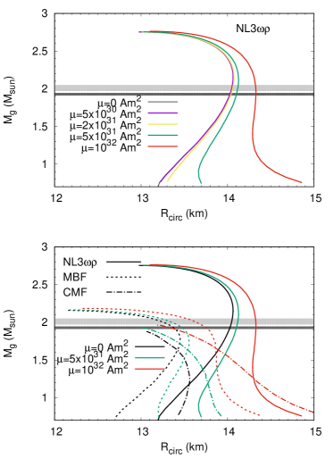
Figure 1: The mass-radius relation for the NL3$\omega\rho$ model for several values of the magnetic dipole moment, $\mu$, (top), and for the three models considered in this paper with three different values of the magnetic dipole moment (bottom).

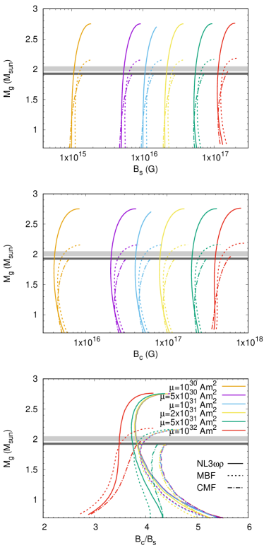
Figure 2: The gravitational mass of several families of stars with different values of the magnetic dipole moment, $\mu$, as a function of the surface polar magnetic field at the pole $B_{s}$ (top), the central magnetic field $B_{c}$ (middle), and the ratio between the central and surface magnetic fields, $B_{c}/B_{s}$, (bottom), for the NL3$\omega\rho$ (solid), MBF (dashed) and CMF (dot-dashed) models.

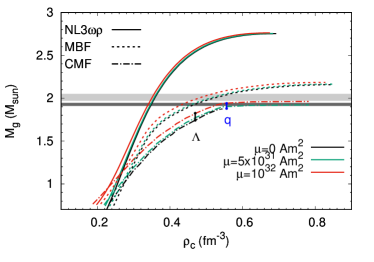
Figure 3: The gravitational mass of several families of stars with different values of the magnetic dipole moment, $\mu$, as a function of the central density for the three models considered in this work. The onset densities of $\Lambda$ and quarks is also shown for the CMF model.

In this subsection, Figs. 1 to 8 show results for several families of stars, using three different EoS: NL3$\omega\rho$, MBF and CMF. According to Haensel et al. (2002), the minimum gravitational mass of cold catalysed stars could be as low as $M\sim 0.1$ M_⊙, whereas according to Goussard et al. (1998); Strobel et al. (1999), lepton-rich matter as found in proto-neutron stars, is unbound for stars with a mass below $\sim 0.9-1.1$ M_⊙. For this reason, in the following, we only show configurations for stars with $M_{g}>0.7$ M_⊙.

In Fig. 1, we show the gravitational mass of several families of stars with different values of the magnetic dipole moment, $\mu$, as a function of the circumferential radius, which characterises the equator of stars coordinate-independently. The horizontal bands indicate the mass uncertainties associated with the PSR J0348 $+0432$ (Antoniadis et al. 2013) (upper) and PSR J1614$-$2230 (Fonseca et al. 2016) (lower) masses. The top panel shows results only for the NL3$\omega\rho$ model. There, one can see that the smaller the mass, the larger the effects of the magnetic field on the stellar structure, as one would expect. A noticeable difference from the non-magnetic case ($\mu=0$) takes place for values of magnetic dipole moment above $\mu=2\times 10^{31}$ Am² and only for low-mass stars. This, therefore, implies that, for higher dipole magnetic moments, stars shall have magnetic fields strong enough to make deformation effects non negligible.

Having this in mind, results for $\mu=0$, $\mu=5\times 10^{31}$ Am², and $\mu=10^{32}$ Am² are displayed for all three models in the bottom panel. The behavior of the magnetised families of stars calculated with the MBF and CMF models is similar to the one calculated with the NL3$\omega\rho$ model. Magnetic dipole moments of the order of $5\times 10^{31}$ Am² and above clearly do have strong effects on the radius of the stars, and this applies to all models.

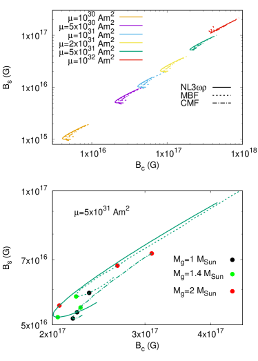
Figure 4: (Top) The correspondence between the central and surface (at the pole) magnetic fields, $B_{c}$ and $B_{s}$, respectively, for the three models. (Bottom) The same as the above panel but only for $\mu=5\times 10^{31}$ Am². The circles show three values of the gravitational mass: $M=1$ M_⊙ (black), $M=1.4$ M_⊙ (green), and $M=2$ M_⊙ (red). The red circle for the CMF model represents the star with the maximum mass, $M=1.92$ M_⊙.

In Fig. 2, we show the gravitational mass of several families of stars with different values of the magnetic dipole moment, $\mu$, as a function of the surface magnetic field at the pole (top panel), the central magnetic field (middle panel), and the ratio between the central and surface magnetic fields, $B_{c}/B_{s}$, (bottom panel), considering the three EoS models. Looking at the top panel, one can see that $\mu=5\times 10^{31}$ Am², a value that gives a significant difference to the $\mu=0$ case in Fig. 1, corresponds to a surface magnetic field at the pole in the range of $\sim 5\times 10^{16}$ G to $10^{17}$ G for the three models and families of stars considered. These surface fields correspond to a central magnetic field in the range of $\sim 2\times 10^{17}$ G to $\sim 4\times 10^{17}$ G, as seen from the middle panel. In addition, the stellar masses are not significantly affected by the magnetic fields, whereas the radius increases with the $B-$ field, as the stars deform into an oblate shape. The bottom panel shows that, for stars with $M_{g}\gtrsim 1$ M_⊙, we have $B_{c}\sim 3-5B_{s}$. The difference is larger for low mass stars and weaker fields, i.e. $\mu<2\times 10^{31}$ Am². This smooth change of magnetic fields inside stars illustrates once more that ad-hoc exponential parametrizations for the magnetic field (Bandyopadhyay et al. 1997) are unrealistic (as already discussed in Dexheimer et al. (2017)), as they produce an increase of several orders of magnitude for the magnetic field inside the stars.

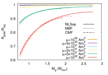
Figure 5: Deviation from spherical symmetry, given by the ratio between the stellar radius at the pole and at the equator, as a function of the gravitational mass for the three models.

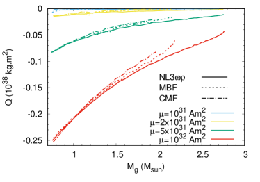
Figure 6: Quadrupole moment of stars as a function of the gravitational mass for the three models.

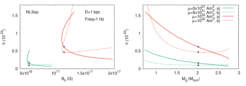
Figure 7: Gravitational wave amplitude from Eq. (1) (a) and from Eq. (5) (b) as a function of the magnetic field at the surface (pole), $B_{s}$, (left), and the gravitational mass (right) for the NL3$\omega\rho$ model. We assumed a family of stars located at a distance of 1 kpc and spinning with a frequency of 1Hz. The black dots correspond to the 2-solar-mass star configurations.

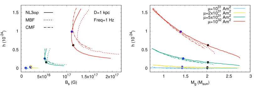
Figure 8: Gravitational wave amplitude from Eq. (1), as a function the magnetic field at the surface (pole), $B_{s}$, (left), and the gravitational mass (right) for the three models. We once more assumed a family of stars located at a distance of 1 kpc and spinning with a frequency of 1Hz. The black dots correspond to $\sim$2-solar-mass star configurations, and the blue ones correspond to 1.4 M_⊙ stars.

The gravitational mass for stellar sequences is plotted as a function of the central density in Fig. 3. The stellar central density is not significantly affected by the magnetic field for the NL3$\omega\rho$: for a 1.8 M_⊙ star the density decreases by $\lesssim 0.01$ fm^-3, while for a 1 M_⊙ star, this difference increases to $\lesssim 0.02$ fm^-3. The CMF stars suffer the larger changes: independently of the stellar mass, as the magnetic field strength changes, the central density decreases by $\lesssim 0.04$ fm^-3 when $\mu$ increases from zero to $\mu=10^{32}$ Am². A strong magnetic field pushes the onset of $\Lambda$s and quarks to stars with masses of $\sim 0.08$ M_⊙ larger than in non-magnetised ones, an effect already discussed in Rabhi et al. (2011). As a consequence, a nucleonic star may suffer a transition to a hybrid star or a hyperonic star when the magnetic fields decays. The onset of hyperons and quarks opens new channels for neutrino emission and, therefore, the possibility of a faster cooling process (Yakovlev et al. 2004; Raduta et al. 2018; Negreiros et al. 2018; Grigorian et al. 2018; Providência et al. 2018). Simultaneously, it also affects the onset of the nucleonic direct Urca process (Fortin et al. 2016; Providência et al. 2018). On the other hand, the conversion of a nucleonic or hyperonic star to a hybrid star could be accompanied by the emission of a reasonable amount of energy, as long as there is a sizable radius change in the involved stellar configurations (Gomes et al. 2018; Dexheimer et al. 2019). In this way, the detection of fast cooling or an energetic event coming from a highly magnetised neutron star could be associated with one of these internal degrees of freedom conversions (Bombaci & Datta 2000; Berezhiani et al. 2003).

In Fig. 4, we show the correspondence between the central magnetic field, $B_{c}$, and the surface magnetic field at the pole, $B_{s}$, for each value of the magnetic dipole moment considered. We observe that the family of stars with the lowest $\mu$ considered has a maximum surface magnetic field of $B_{s}\sim 2\times 10^{15}$ G. This is also seen on the top panel of Fig. 2. The sequence of stars with the highest $\mu$ has a corresponding $B_{s}\sim 2\times 10^{17}$ G and a central magnetic field of the order of $10^{18}$ G. The behaviour of $B_{s}$ versus $B_{c}$ is not monotonic and, in the bottom panel, the results for $\mu=5\times 10^{31}$ Am² are shown with more detail for the three EoS considered in this work. The overall behavior is model-independent, although the quantitative behaviour does depend on the EoS considered. In the bottom panel, the stars with $M=1.0,1.4$ and 2 M_⊙ have been identified. The minimum $B_{c}$ of the curve occurs for a star with a mass of the order of 1.4 M_⊙ and corresponds to the star where the mass-radius curve changes curvature. For stars with a mass greater or smaller than $\sim 1.4$ M_⊙, the surface field increases monotonically with the central magnetic field.

In Fig. 5, we show the stars’ deviation from spherical symmetry, given by the ratio between the radius at the magnetic pole and the radius at the equator, as a function of the gravitational mass. We see that for the lowest magnetic dipole moments considered the deformation is very small and it happens only for the low-mass stars, i.e., with $M<1$ M_⊙. For a 1 M_⊙ star, the difference between the polar and equatorial radii is below 1$\%$. Deformation appears for stars with higher magnetic dipole moments. This allows us to conclude that we only have significant deformation for values of the magnetic dipole moment $\mu\gtrsim 2\times 10^{31}$ Am², which correspond to a surface magnetic field of $B_{s}\gtrsim 2-4$ ($10^{16}$ G), and $B_{c}=1-2$ ($10^{17}$ G) (see Fig. 2).

We can also analyse the deformation of stars by looking at their quadrupole moments. Fig. 6 shows the quadrupole moment of the families of stars considered in this study as a function of the gravitational mass. As expected, the results for the quadrupole moment are in agreement with the ones shown for the deformation: it becomes non-negligible only for $\mu\gtrsim 2\times 10^{31}$ Am² (see the previous figure).

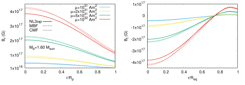
Figure 9: The radial component of the magnetic field (left) and the tangential component of the magnetic field (right) as a function of the normalised radius for the three models considering only stars with fixed baryon mass $M_{b}=1.6$ M_⊙.

It has been shown (Bonazzola & Gourgoulhon 1996) that, for a slightly deformed star, the amplitude of gravitational waves emitted is given by

$$h_{0}=-\dfrac{6G}{c^{4}}Q\dfrac{\Omega^{2}}{D}\,,$$ (1)

where $G$ is the gravitational constant, $c$ the speed of light, $Q$ the quadrupole moment, $D$ the distance to the star, and $\Omega$ the rotational velocity of the star. Another way to estimate the gravitational wave amplitude is from the magnetic field induced deformation (Bonazzola & Gourgoulhon 1996), where considering an incompressible magnetised fluid, the quadrupole moment can be written as

$$Q=-\dfrac{\mu_{0}\mu^{2}}{16\pi^{2}G\rho R^{3}}\,,$$ (2)

where $\mu_{0}$ is the magnetic permeability of free space, so that the ellipticity, $\epsilon_{B}$, and the moment of inertia, $I$, of the star are given by

$$\epsilon_{B} = \dfrac{15\pi B_{s}^{2}R_{circ}^{4}}{12\mu_{0}GM_{g}^{2}}\,,$$ (3)

$$I = \dfrac{2}{5}M_{g}R_{circ}^{2}\,,$$ (4)

considering uniform density throughout the star, and approximating the moment of inertia to the one of a sphere. The gravitational wave amplitude can then be expressed as

$$h_{0}=\dfrac{16\pi^{2}G\epsilon_{B}I}{c^{4}DP^{2}}\,,$$ (5)

where $P$ is the period of rotation of the star, $P=2\pi/\Omega$. An estimation of the amplitude of gravitational waves emitted by these stars is done by setting the distance to 1 kpc (the distances to the pulsars PSR J1614-2230, Vela, and Crab are $\sim 1.2$ kpc , $\sim 0.5$ kpc, and $\sim 2$ kpc, respectively) and the frequency $f=1/P=1$ Hz. Results are shown in the next two figures.

In Fig. 7, we show the gravitational wave (GW) amplitude calculated using the expressions in Eqs. (1) and (5), for the NL3$\omega\rho$ model. We also mark the 2 M_⊙ star configurations. Even though the two curves behave similarly, they do not give the same results and, in fact, the difference is significant: for the 2 M_⊙ case, with $\mu=5\times 10^{31}$ Am², we obtain $h_{0}=0.15\times 10^{-24}$ for Eq. (1) and $h_{0}=0.1\times 10^{-24}$ for Eq. (5). The difference increases when we consider the $\mu=10^{32}$ Am² case: $0.65\times 10^{-24}$ for Eq. (1) and $0.45\times 10^{-24}$ for Eq. (5). The estimation obtained from Eq. (5) is worse for the lower mass stars, which have the larger deformations. This illustrates that using an approximate expression, as in Eq. (5), that considers stars with uniform density and a moment of inertia given by the one of a sphere, produces different results and emphasizes the fact that these approaches should be considered with care when calculating sensitive quantities like GW amplitudes.

In the following, GW amplitudes are estimated from Eq. (1) for the three models we have considered. In Fig. 8, the gravitational wave amplitude is shown as a function of the magnetic field at the surface, $B_{s}$, and as a function of the gravitational mass, for a family of stars located at a distance of 1 kpc and spinning with a frequency of 1 Hz. The black dots correspond to 2 M_⊙ configurations and the blue ones correspond to 1.4 M_⊙ stars.

Besides calculating the GW amplitude, we can also estimate the characteristic strain, $S$, the actual quantity measured by the interferometer detectors. It is defined as the product between the GW amplitude and the square root of the integration time (Bonazzola & Gourgoulhon 1996; Moore et al. 2015): $S=h_{0}\sqrt{P}$. If we assume that data was collected during a period of three years, i.e., $\sqrt{P}\sim 10^{4}$ s, the characteristic strain becomes proportional to GW amplitude by a factor of $10^{4}$.

This means that for a star with $B_{s}=2\times 10^{16}$ G, $M_{g}=2$ M_⊙, at 1 kpc away and spinning at 1 Hz, we obtain $h_{0}=0.15\times 10^{-24}$ and $S=1.5\times 10^{-21}$ Hz^-1/2. This value could indeed still be detected by detectors like BBO, DECIGO, ALIA. Detectors LIGO and Virgo detect a higher frequency range, $f>30$ Hz (Christopher Moore & Berry 2019).

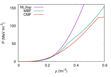
Figure 10: Equation of state for the three models considered in this work.

3.2 Single-star configurations with $M_{b}=1.6$ M_⊙

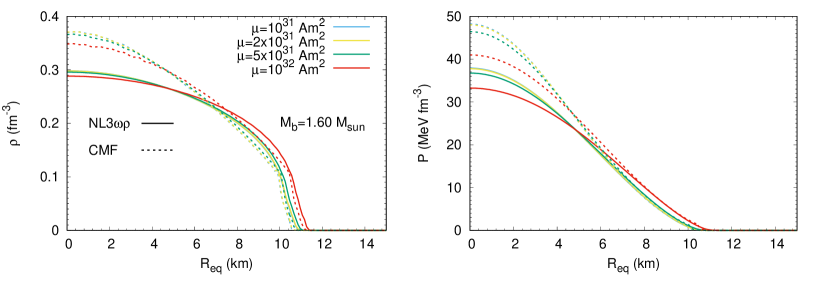
Figure 11: Profiles of the stars: (left) baryon number density and (right) pressure calculated in the equatorial plane for the three models considered in this work.

In this subsection, we discuss the properties of magnetised stars with a fixed baryonic mass of 1.6 M_⊙, with different magnetic dipole moments, $\mu$. Stars with this baryonic mass have a gravitational mass of the order of 1.4 M_⊙. The radial component of the magnetic field (left) and the tangential component of the magnetic field (right) are plotted in Fig. 9 as a function of the normalised radius for different values of $\mu$. The radial component of $B$, $B_{r}$, is calculated at $(r,\theta=0,\phi=0)$ (polar) and the tangential (to the equatorial surface) component, $B_{t}$, is calculated at $(r,\theta=\pi/2,\phi=0)$. The change of direction of the tangential field occurs for all magnetic momenta at around $R_{eq}/4$ from the surface of the star.

As expected, the higher the $\mu$, the higher the magnetic field magnitude. However, it is interesting to see how the intensity of the field depends on the model: NL3$\omega\rho$ has the smallest radial and tangential component absolute values, while the other two models show similar magnitudes. This behavior comes from the fact that the CMF model has the softest EoS and gives rise to larger magnetic field intensities for the same magnetic dipole moment (see Fig. 10, where the three EoS used in this work are represented). From Fig. 3, one can see that stars with $M\sim 1.4$ M_⊙ have similar central densities for models CMF and MBF below $\rho=0.4$ fm^-3. CMF is the softest EoS above saturation and develops the strongest fields in the interior of the star. Below saturation density, however, CMF is closer to NL3$\omega\rho$ and it is the MBF model, with the softest low density EoS, that develops the strongest surface fields. In the past, it was shown that the compactness of stars is directly related to the strength of central magnetic fields, through the softness of the EoS (Gomes et al. 2017). Our results indicate that the relation between the magnetic field in the center of the star and the one on the surface, as discussed in Fig. 4, is defined by the properties of the EoS both at the crust and in the core.

The effect of magnetic fields on the structure of stars is also clearly shown in Fig.  11, where the profiles of stars with different magnetic field configurations are plotted for models NL3$\omega\rho$ and CMF: the density, and the pressure are calculated at the equatorial plane. Effects of the magnetic field are i) a decrease of the density and pressure in the core of the star and ii) an increase of the pressure at the surface. As a consequence, matter is pushed outwards and the radius of the star increases. For $\mu=5\times 10^{31}$ Am², the effect is already seen but it is still small. For $\mu=10^{32}$ Am², a decrease of the density in the core has as a direct consequence: the suppression of the possible onset of non-nucleonic degrees of freedom, hyperons or a quark phase, as already discussed in Refs. (Franzon et al. 2015, 2016a; Gomes et al. 2017). This explains some results shown in Fig. 1 for the CMF model: in the presence of a magnetic field, the onset of $\Lambda$s and quark matter occur in stars with larger masses.

Let us now consider a star described by the CMF model with strong magnetic field in the interior that has a gravitational (or baryonic) mass above the maximum mass possible for a non-magnetised or weakly magnetised star. A direct consequence of the instability occurring when the magnetic field decays to values that allow for higher central stellar densities, and a possible onset of quark matter, is that the star becomes unstable and decays into a low mass black hole. This transition could be possibly identified by the observation of a gamma-ray burst.

4 Final Remarks

In the present work, we have calculated the magnetic field strength above which the deformation of the neutron star structure is at least 2%, which is already non-negligible. We have considered three representative relativistic mean field models to describe the EoS of neutron stars with diverse compositions (nucleonic, hyperonic and hybrid). The calculations for the structure of stars were performed within the general relativistic framework implemented in the publicly available Langage Objet pour la RElativité NumériquE (LORENE) library (Bonazzola et al. 1993; Bocquet et al. 1995).

Our calculation was undertaken by quantifying the deformation due to the magnetic field, in particular, the relation between the polar and equatorial radii, and defining the magnetic dipole moment that causes a difference below $\sim 1-2\%$, corresponding to a magnetic field of the order of $\sim 10^{17}$ G in the center and $\sim 5\times 10^{16}$ G at the surface. It has been shown that, within the adopted formalism, the magnetic field developed inside the star, and at the surface, depends on the EoS. For a fixed magnetic dipole moment, stronger magnetic fields are obtained for a softer EoS. Quantitatively, we have found that, for the magnetic field range studied, the relation between these two quantities to be $B_{c}\sim 3-5\times B_{s}$, with the relation being dependent on the EoS and the stellar mass.

The determination of the threshold magnetic field for deformed neutron stars was undertaken in two equivalent approaches. In the polar versus equatorial radii method, we have identified the magnetic dipole moment that causes a difference $\sim 1-2\%$ between both. In the quadrupole moment method, we use the neutron star quadrupole moment to quantify a deformation of a similar magnitude. We find that the limiting magnetic field for which the integration of the TOV equations still gives realistic results for the structure of magnetised neutron stars is, in general, model independent.

We report that for stars with masses below $1.5\,\mathrm{M_{\odot}}$, a dipole magnetic moment of $\sim 2\times 10^{31}\,\mathrm{Am^{2}}$, which corresponds to a surface magnetic field of the order of $\sim 2\times 10^{16}$ G and a central magnetic field of $\sim 8\times 10^{16}$ G, is enough to cause deformation above $1-2\%$ on stars. The same effect is seen for all masses, when stars are described with a dipole magnetic moment of $\sim 5\times 10^{31}\,\mathrm{Am^{2}}$, corresponding to a surface magnetic field of the order of $\sim 5\times 10^{16}$ G and a central magnetic field of $\sim 2-4\times 10^{17}$ G. For the analysis carried out in this work, our results are independent of the model and the composition of stars.

We have also discussed under which conditions the decay of the magnetic field could give rise to the collapse of the neutron star or the onset of hyperons. Let us refer to the fact that the onset of hyperons inside stars has important effects on the cooling of the star, not only by affecting the onset density of the nucleonic electron direct Urca process, but also by opening new direct Urca channels involving hyperons.

For a matter of completeness, we have investigated the magnetic field distribution inside individual $M_{b}=1.6$ M_⊙ stars, both in equatorial and radial directions, showing that for the case of approximately spherical stars, all the models and compositions present a quantitative and qualitative similar behavior. The models discussed in this work present different baryon density distributions, which is a direct consequence of the degree of stiffness of their EoS.

Finally, we have compared two methods for determining the gravitational wave amplitude for single stars, considering both the case of approximately spherical stars (slightly deformed) and stars with induced deformation through magnetic effects. We show that, even for the lowest magnetic field that generates a relevant deformation, calculations for the gravitational wave amplitude using these two methods never agree. The disagreement between the two methods increases for higher magnetic field amplitudes, as the stars become more deformed. Therefore, we emphasise that such calculations should be carried out cautiously, especially for highly magnetised neutron stars.

References

- Antoniadis et al. (2013) Antoniadis, J., Freire, P. C. C., Wex, N., et al. 2013, Science (New York, N.Y.), 340, 448, 1233232
- Avancini et al. (2012) Avancini, S. S., Menezes, D. P., Pinto, M. B., & Providencia, C. 2012, Phys. Rev., D85, 091901
- Bandyopadhyay et al. (1997) Bandyopadhyay, D., Chakrabarty, S., & Pal, S. 1997, Phys. Rev. Lett., 79, 2176
- Baym et al. (1971) Baym, G., Pethick, C., & Sutherland, P. 1971, ApJ, 170, 299
- Bejger et al. (2017) Bejger, M., Blaschke, D., Haensel, P., Zdunik, J. L., & Fortin, M. 2017, Astron. Astrophys., 600, A39
- Berezhiani et al. (2003) Berezhiani, Z., Bombaci, I., Drago, A., Frontera, F., & Lavagno, A. 2003, Astrophys. J., 586, 1250
- Bethe & Johnson (1974) Bethe, H. A. & Johnson, M. B. 1974, Nuclear Physics A, 230, 1
- Bocquet et al. (1995) Bocquet, M., Bonazzola, S., Gourgoulhon, E., & Novak, J. 1995, Astron. Astrophys., 301, 757
- Bombaci & Datta (2000) Bombaci, I. & Datta, B. 2000, Astrophys. J., 530, L69
- Bonazzola & Gourgoulhon (1996) Bonazzola, S. & Gourgoulhon. 1996, Astron. Astrophys., 312, 675
- Bonazzola et al. (1998) Bonazzola, S., Gourgoulhon, E., & Marck, J.-A. 1998, Phys. Rev. D, 58, 104020
- Bonazzola et al. (1993) Bonazzola, S., Gourgoulhon, E., Salgado, M., & Marck, J. A. 1993, Astron. Astrophys., 278, 421
- Broderick et al. (2000) Broderick, A. E., Prakash, M., & Lattimer, J. M. 2000, Astrophys. J., 537, 351
- Broderick et al. (2002) Broderick, A. E., Prakash, M., & Lattimer, J. M. 2002, Phys. Lett., B531, 167
- Cai et al. (2015) Cai, B.-J., Fattoyev, F. J., Li, B.-A., & Newton, W. G. 2015, Phys. Rev., C92, 015802
- Cardall et al. (2001) Cardall, C. Y., Prakash, M., & Lattimer, J. M. 2001, Astrophys. J., 554, 322
- Chakrabarty (1996) Chakrabarty, S. 1996, Phys. Rev., D54, 1306
- Chakrabarty et al. (1997) Chakrabarty, S., Bandyopadhyay, D., & Pal, S. 1997, Phys. Rev. Lett., 78, 2898
- Chamel et al. (2012) Chamel, N., Pavlov, R. L., Mihailov, L. M., et al. 2012, Phys. Rev., C86, 055804
- Chamel et al. (2015) Chamel, N., Stoyanov, Z. K., Mihailov, L. M., et al. 2015, Phys. Rev., C91, 065801
- Chatterjee et al. (2015) Chatterjee, D., Elghozi, T., Novak, J., & Oertel, M. 2015, Mon. Not. Roy. Astron. Soc., 447, 3785
- Chatterjee et al. (2018) Chatterjee, D., Gulminelli, F., & Menezes, D. P. 2018 [arXiv:1812.05879]
- Chatterjee & Vidana (2016) Chatterjee, D. & Vidana, I. 2016, Eur. Phys. J., A52, 29
- Chatterjee & Vidaña (2016) Chatterjee, D. & Vidaña, I. 2016, Eur. Phys. J., A52, 29
- Christopher Moore & Berry (2019) Christopher Moore, R. C. & Berry, C. 2019, http://gwplotter.com
- Ciolfi (2014) Ciolfi, R. 2014, Astron. Nachr., 335, 624
- Costa et al. (2014) Costa, P., Ferreira, M., Hansen, H., Menezes, D. P., & Providência, C. 2014, Phys. Rev., D89, 056013
- Dexheimer et al. (2017) Dexheimer, V., Franzon, B., Gomes, R. O., et al. 2017, Phys. Lett., B773, 487
- Dexheimer et al. (2018) Dexheimer, V., Gomes, R. d. O., Schramm, S., & Pais, H. 2018 [arXiv:1810.06109]
- Dexheimer et al. (2019) Dexheimer, V., Soethe, L. T. T., Roark, J., et al. 2019, arXiv e-prints [arXiv:1901.03252]
- Dexheimer & Schramm (2010) Dexheimer, V. A. & Schramm, S. 2010, Phys. Rev., C81, 045201
- Diaz Alonso (1985) Diaz Alonso, J. 1985, Phys. Rev. D, 31, 1315
- Drago et al. (2016) Drago, A., Lavagno, A., Pagliara, G., & Pigato, D. 2016, Eur. Phys. J., A52, 40
- Fang et al. (2016) Fang, J., Pais, H., Avancini, S., & Providência, C. 2016, Phys. Rev. C, 94, 062801
- Fang et al. (2017) Fang, J., Pais, H., Pratapsi, S., et al. 2017, Phys. Rev. C, 95, 045802
- Fang et al. (2017) Fang, J., Pais, H., Pratapsi, S., & Providência, C. 2017, Phys. Rev., C95, 062801
- Ferreira et al. (2014) Ferreira, M., Costa, P., Menezes, D. P., Providência, C., & Scoccola, N. 2014, Phys. Rev., D89, 016002, [Addendum: Phys. Rev.D89,no.1,019902(2014)]
- Fonseca et al. (2016) Fonseca, E., Pennucci, T. T., Ellis, J. A., et al. 2016, ApJ, 832, 167
- Fortin et al. (2016) Fortin, M., Providência, C., Raduta, A. R., et al. 2016, Phys. Rev., C94, 035804
- Fortin et al. (2018) Fortin, M., Taranto, G., Burgio, G. F., et al. 2018, Mon. Not. Roy. Astron. Soc., 475, 5010
- Franzon et al. (2015) Franzon, B., Dexheimer, V., & Schramm, S. 2015, Mon. Not. Roy. Astron. Soc., 456, 2937
- Franzon et al. (2016a) Franzon, B., Dexheimer, V., & Schramm, S. 2016a, Phys. Rev., D94, 044018
- Franzon et al. (2016b) Franzon, B., Gomes, R. O., & Schramm, S. 2016b, Mon. Not. Roy. Astron. Soc., 463, 571
- Frieben & Rezzolla (2012) Frieben, J. & Rezzolla, L. 2012, Mon. Not. Roy. Astron. Soc., 427, 3406
- Gomes et al. (2018) Gomes, R. O., Dexheimer, V., Han, S., & Schramm, S. 2018 [arXiv:1810.07046]
- Gomes et al. (2015) Gomes, R. O., Dexheimer, V., Schramm, S., & Vasconcellos, C. A. Z. 2015, Astrophys. J., 808, 8
- Gomes et al. (2017) Gomes, R. O., Franzon, B., Dexheimer, V., & Schramm, S. 2017, Astrophys. J., 850, 20
- Gourgoulhon (2012) Gourgoulhon, E., ed. 2012, Lecture Notes in Physics, Berlin Springer Verlag, Vol. 846, 3+1 Formalism in General Relativity
- Goussard et al. (1998) Goussard, J. O., Haensel, P., & Zdunik, J. L. 1998, Astron. Astrophys., 330, 1005
- Grigorian et al. (2018) Grigorian, H., Voskresensky, D. N., & Maslov, K. A. 2018, Nucl. Phys., A980, 105
- Grill et al. (2014) Grill, F., Pais, H., Providência, C., Vidaña, I., & Avancini, S. S. 2014, Phys. Rev. C, 90, 045803
- Haensel et al. (1981) Haensel, P., Proszynski, M., & Kutschera, M. 1981, Astron. Astrophys., 102, 299
- Haensel et al. (2002) Haensel, P., Zdunik, J. L., & Douchin, F. 2002, Astron. Astrophys., 385, 301
- Hebeler et al. (2013) Hebeler, K., Lattimer, J. M., Pethick, C. J., & Schwenk, A. 2013, ApJ, 773, 11
- Kaspi & Beloborodov (2017) Kaspi, V. M. & Beloborodov, A. 2017, Ann. Rev. Astron. Astrophys., 55, 261
- Kondratyev et al. (2001) Kondratyev, V. N., Maruyama, T., & Chiba, S. 2001, Astrophys. J., 546, 1137
- Lai & Shapiro (1991) Lai, D. & Shapiro, S. L. 1991, Astrophysical Journal, 383, 745
- Lander & Jones (2018) Lander, S. K. & Jones, D. I. 2018 [arXiv:1807.01289]
- LORENE (2019) LORENE. 2019, https://lorene.obspm.fr
- Lugones & Grunfeld (2018) Lugones, G. & Grunfeld, A. G. 2018, arXiv e-prints [arXiv:1811.09954]
- Mereghetti et al. (2015) Mereghetti, S., Pons, J., & Melatos, A. 2015, Space Sci. Rev., 191, 315
- Moore et al. (2015) Moore, C. J., Cole, R. H., & Berry, C. P. L. 2015, Class. Quant. Grav., 32, 015014
- Negreiros et al. (2013) Negreiros, R., Schramm, S., & Weber, F. 2013, Phys. Lett., B718, 1176
- Negreiros et al. (2018) Negreiros, R., Tolos, L., Centelles, M., Ramos, A., & Dexheimer, V. 2018, Astrophys. J., 863, 104
- Oppenheimer & Volkoff (1939) Oppenheimer, J. R. & Volkoff, G. M. 1939, Phys. Rev., 55, 374
- Pais & Providência (2016) Pais, H. & Providência, C. 2016, Phys. Rev. C, 94, 015808
- Pandharipande (1971) Pandharipande, V. R. 1971, Nuclear Physics A, 174, 641
- Patiño et al. (2018) Patiño, J. T., Bauer, E., & Vidaña, I. 2018 [arXiv:1809.00688]
- Pearson et al. (2012) Pearson, J. M., Chamel, N., Goriely, S., & Ducoin, C. 2012, Phys. Rev., C85, 065803
- Potekhin & Chabrier (2013) Potekhin, A. Y. & Chabrier, G. 2013, Astron. Astrophys., 550, A43
- Potekhin & Chabrier (2018) Potekhin, A. Y. & Chabrier, G. 2018, Astron. Astrophys., 609, A74
- Potekhin et al. (2013) Potekhin, A. Y., Fantina, A. F., Chamel, N., Pearson, J. M., & Goriely, S. 2013, Astron. Astrophys., 560, A48
- Providência et al. (2018) Providência, C., Fortin, M., Pais, H., & Rabhi, A. 2018 [arXiv:1811.00786]
- Rabhi et al. (2011) Rabhi, A., Panda, P. K., & Providencia, C. 2011, Phys. Rev., C84, 035803
- Rabhi & Providencia (2010) Rabhi, A. & Providencia, C. 2010, J. Phys., G37, 075102
- Raduta et al. (2017) Raduta, A. R., Sedrakian, A., & Weber, F. 2017 [arXiv:1712.00584]
- Raduta et al. (2018) Raduta, A. R., Sedrakian, A., & Weber, F. 2018, Mon. Not. Roy. Astron. Soc., 475, 4347
- Roark & Dexheimer (2018) Roark, J. & Dexheimer, V. 2018, Phys. Rev., C98, 055805
- Ruester et al. (2006) Ruester, S. B., Hempel, M., & Schaffner-Bielich, J. 2006, Phys. Rev., C73, 035804
- Salgado et al. (1994) Salgado, M., Bonazzola, S., Gourgoulhon, E., & Haensel, P. 1994, Astron. Astrophys., 291, 155
- Sharma et al. (2015) Sharma, B. K., Centelles, M., Viñas, X., Baldo, M., & Burgio, G. F. 2015, Astron. Astrophys., 584, A103
- Sinha & Sedrakian (2015) Sinha, M. & Sedrakian, A. 2015, Phys. Rev., C91, 035805
- Stein et al. (2016) Stein, M., Maruhn, J., Sedrakian, A., & Reinhard, P. G. 2016, Phys. Rev., C94, 035802
- Strobel et al. (1999) Strobel, K., Schaab, C., & Weigel, M. K. 1999, Astron. Astrophys., 350, 497
- Suh & Mathews (2001) Suh, I.-S. & Mathews, G. J. 2001, Astrophys. J., 546, 1126
- Thompson & Duncan (1995) Thompson, C. & Duncan, R. C. 1995, Mon. Not. Roy. Astron. Soc., 275, 255
- Thompson & Duncan (1996) Thompson, C. & Duncan, R. C. 1996, Astrophys. J., 473, 322
- Tolman (1939) Tolman, R. C. 1939, Phys. Rev., 55, 364
- Uryu et al. (2014) Uryu, K., Gourgoulhon, E., Markakis, C., et al. 2014, Phys. Rev., D90, 101501
- Yakovlev et al. (2004) Yakovlev, D. G., Levenfish, K. P., Potekhin, A. Y., Gnedin, O. Y., & Chabrier, G. 2004, Astron. Astrophys., 417, 169
- Yuan & Zhang (1999) Yuan, Y. F. & Zhang, J. L. 1999, Astrophys. J., 525, 950
- Zdunik & Haensel (2013) Zdunik, J. L. & Haensel, P. 2013, Astron. Astrophys., 551, A61