Total Variation and Mean Curvature PDEs on $\mathbb{R}^{d}\rtimes S^{d-1}$

Abstract

Total variation regularization and total variation flows (TVF) have been widely applied for image enhancement and denoising. To include a generic preservation of crossing curvilinear structures in TVF we lift images to the homogeneous space $\mathbb{M}=\mathbb{R}^{d}\rtimes S^{d\!-\!1}$ of positions and orientations as a Lie group quotient in $SE(d)$. For $d=2$ this is called ‘total roto-translation variation’ by Chambolle & Pock. We extend this to $d=3$, by a PDE-approach with a limiting procedure for which we prove convergence. We also include a Mean Curvature Flow (MCF) in our PDE model on $\mathbb{M}$. This was first proposed for $d=2$ by Citti et al. and we extend this to $d=3$. Furthermore, for $d=2$ we take advantage of locally optimal differential frames in invertible orientation scores (OS).

We apply our TVF and MCF in the denoising/enhancement of crossing fiber bundles in DW-MRI. In comparison to data-driven diffusions, we see a better preservation of bundle boundaries and angular sharpness in fiber orientation densities at crossings. We support this by error comparisons on a noisy DW-MRI phantom. We also apply our TVF and MCF in enhancement of crossing elongated structures in 2D images via OS, and compare the results to nonlinear diffusions (CED-OS) via OS.

1 Introduction

In the last decade, many PDE-based image analysis techniques for tracking and enhancement of curvilinear structures took advantage of lifting the image data to the homogeneous space $\mathbb{M}=\mathbb{R}^{d}\rtimes S^{d\!-\!1}$ of d-dimensional positions and orientations, cf. ​[14, 10, 34, 6, 4, 8]. The precise definition of this homogeneous space follows in the next subsection. Set-wise it can be seen as a Cartesian product $\mathbb{M}=\mathbb{R}^{d}\times S^{d\!-\!1}$. Geometrically it can be equipped with a roto-translation equivariant geometry and topology beyond the usual isotropic Riemannian setting.

Typically, these PDE-based image analysis techniques involve flows that implement morphological and (non)linear scale spaces or solve variational models. The key advantage of extending the image domain from $\mathbb{R}^{d}$ to the higher dimensional lifted space $\mathbb{M}$ is that the PDE-flows do not suffer from crossings as fronts can pass without collision. This idea was shown for image enhancement in [21, 9]. In [21] the method of coherence enhancing diffusion (CED) [35], was lifted to $\mathbb{M}$ in a diffusion flow method called ”coherence enhancing diffusion on invertible orientation scores” (CED-OS), that is recently generalized to 3D [24]. Also for geodesic tracking methods, it helps that crossing line structures are disentangled in the lifted data. Geodesic flows prior to steepest descent also rely on (related [32, 5, 8]) PDEs on $\mathbb{M}$ commuting with roto-translations. They can account for crossings/bifurcations/corners [4, 18, 8].

Nowadays PDE-flows on orientation lifts of 3D images are indeed relevant for applications such as fiber enhancement [12, 34, 30, 15] and fiber tracking [29] in Diffusion-Weighted Magnetic Resonance Imaging (DW-MRI), and in enhancement [24] and tracking [11] of blood vessels in 3D images.

As for PDE-based image denoising and enhancement, total variation flows (TVF) are more popular than nonlinear diffusion flows. Recently, Chambolle & Pock generalized TVF from $\mathbb{R}^{2}$ to $\mathbb{M}=\mathbb{R}^{2}\times S^{1}$, via ‘total roto-translation variation’ (TV-RT) flows [8] of 2D images. They employ (a)symmetric Finslerian geodesic models on $\mathbb{M}$ cf. ​[18]. As TVF falls short on invariance w.r.t. monotonic co-domain transforms, we also consider a Mean Curvature Flow (MCF) variant in our PDE model on $\mathbb{M}$, as proposed for 2D (i.e. $d=2$) by Citti et al. [9].

To get a visual impression of how such PDE-based image processing on lifted images (orientation scores) works, for the case of tracking and enhancement of curvilinear structures in images see Fig. ​1. In the 3rd row of Fig. ​1, and henceforth, we visualize a lifted image $U:\mathbb{R}^{3}\rtimes S^{2}\to\mathbb{R}^{+}$ by a grid of angular profiles $\{\,\mu\,U(\mathbf{x},\mathbf{n})\,\mathbf{n}\;|\;\mathbf{x}\in\mathbb{Z}^{3},\mathbf{n}\in S^{2}\,\}$, with fixed $\mu>0$.

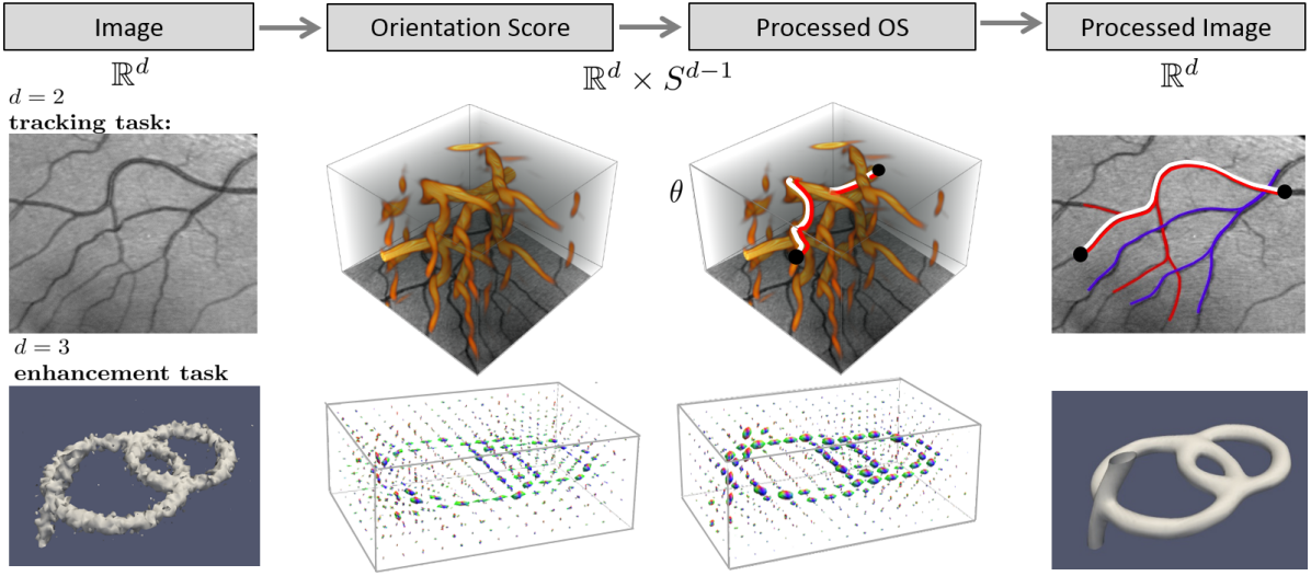
Figure 1: Instead of direct PDE-based processing of an image, we apply PDE-based processing on a lifted image $U:\mathbb{R}^{d}\rtimes S^{d-1}\to\mathbb{R}$ (e.g. an orientation score: OS). The OS is obtained by convolving the image with a set of rotated wavelets allowing for stable reconstruction [14, 4, 24]. 2nd row: Vessel-tracking in a 2D image via geodesic PDE-flows in OS that underly TVF: [4, 18, 8], with $\mathbf{n}=(\cos\theta,\sin\theta)^{T}\in S^{1}$. 3rd row: CED-OS diffusion of a 3D image [24, 17] visualized as a field of angular profiles. In this article we study image enhancement and denoising via TVF and MCF on $\mathbb{M}=\mathbb{R}^{d}\rtimes S^{d\!-\!1}$ and compare to nonlinear diffusion methods on $\mathbb{M}$ (like CED-OS).

The main contributions of this article are:

• We set up a geometric PDE flow framework on $\mathbb{M}$ including TVF, MCF, and diffusion. We tackle the PDEs by a basic limiting procedure. For TVF we prove convergence via Gradient flow theory by Brezis-Komura [7, 1].

• We extend TVF on $\mathbb{M}$ [8], and MCF on $\mathbb{M}$ [9] to the 2D and 3D setting.

• We apply TVF and MCF in the denoising and enhancement of crossing fiber bundles in fiber orientation density functions (FODF) of DW-MRI data. In comparison to data-driven diffusions, we show a better preservation of bundle boundaries and angular sharpness with TVF and MCF. We support this observation by error comparisons on a noisy DW-MRI phantom.

• We include locally optimal differential frames (LAD) [17] in invertible orientation scores (OS), and propose crossing-preserving denoising methods TVF-OS, MCF-OS. We show benefits of LAD inclusion on 2D data.

• We compare TVF-OS, MCF-OS to CED-OS on 2D images.

2 Theory

2.1 The Homogeneous Space $\mathbb{M}$ of Positions and Orientations

Set $d\in\{2,3\}$. Consider the rigid body motion group, $SE(d)=\mathbb{R}^{d}\rtimes SO(d)$. It acts transitively on $\mathbb{R}^{d}\times S^{d\!-\!1}$ by

$$g\odot(\mathbf{x}^{\prime},\mathbf{n}^{\prime})=(\mathbf{R}\mathbf{x}^{\prime}+\mathbf{x},\mathbf{R}\mathbf{n}^{\prime}),\textrm{ for all }g=(\mathbf{x},\mathbf{R})\in SE(d),\ (\mathbf{x}^{\prime},\mathbf{n}^{\prime})\in\mathbb{R}^{d}\times S^{d\!-\!1}.$$

Now set $\mathbf{a}\in S^{d-1}$ as an a priori reference axis, say $\mathbf{a}=(1,0)$ if $d=2$ and $\mathbf{a}=\mathbf{e}_{z}=(0,0,1)^{T}$ if $d=3$. The homogeneous space of positions and orientations is the partition of left-cosets:

$$\mathbb{M}:=\mathbb{R}^{d}\rtimes S^{d\!-\!1}:=SE(d)/H,$$

in $SE(d)$ and $H=\{g\in SE(d)\;|\;g\odot(\mathbf{0},\mathbf{a})=(\mathbf{0},\mathbf{a})\}$. For $d=2$ we have $\mathbb{M}\equiv SE(2)$. For $d=3$ we have that

$$H=\{h_{\alpha}:=(\mathbf{0},\mathbf{R}_{\mathbf{a},\alpha})\;|\;\alpha\in[0,2\pi)\},$$ (1)

where $\mathbf{R}_{\mathbf{a},\alpha}$ denotes a (counter-clockwise) rotation around $\mathbf{a}=\mathbf{e}_{z}$. Recall that by the definition of the left-cosets one has $H=\{\mathbf{0}\}\times SO(2),\textrm{ and }g_{1}\sim g_{2}\Leftrightarrow g_{1}^{-1}g_{2}\in H$. This means that for $g_{1}=(\mathbf{x}_{1},\mathbf{R}_{1})$, $g_{2}=(\mathbf{x}_{2},\mathbf{R}_{2})$ one has

$$g_{1}\sim g_{2}\Leftrightarrow\mathbf{x}_{1}=\mathbf{x}_{2}\textrm{ and }\exists_{\alpha\in[0,2\pi)}\;:\;\mathbf{R}_{1}=\mathbf{R}_{2}\mathbf{R}_{\mathbf{a},\alpha}.$$

The equivalence classes $[g]=\{g^{\prime}\in SE(3)\;|\;g^{\prime}\sim g\}$ are usually just denoted by $\mathbf{p}=(\mathbf{x},\mathbf{n})$ as they consist of all rigid body motions $g=(\mathbf{x},\mathbf{R}_{\mathbf{n}})$ that map reference point $(\mathbf{0},\mathbf{a})$ onto $(\mathbf{x},\mathbf{n})\in\mathbb{R}^{3}\rtimes S^{2}$ :

$$g\odot(\mathbf{0},\mathbf{a})=(\mathbf{x},\mathbf{n}).$$ (2)

On tangent bundle $T(\mathbb{M})=\{(\mathbf{p},\dot{\mathbf{p}})\;|\;\mathbf{p}\in\mathbb{M},\dot{\mathbf{p}}\in T_{\mathbf{p}}(\mathbb{M})\}$ we set metric tensor:

$$\begin{array}[]{l}\left.\mathcal{G}_{\gothic{e}}\right|_{\mathbf{p}}(\dot{\mathbf{p}},\dot{\mathbf{p}})=D_{S}^{-1}|\dot{\mathbf{x}}\cdot\mathbf{n}|^{2}+D_{A}^{-1}\|\dot{\mathbf{n}}\|^{2}+\gothic{e}^{-2}D_{S}^{-1}\|\dot{\mathbf{x}}\wedge\mathbf{n}\|^{2},\\[5.0pt] \textrm{for all }\mathbf{p}=(\mathbf{x},\mathbf{n})\in\mathbb{M},\dot{\mathbf{p}}=(\dot{\mathbf{x}},\dot{\mathbf{n}})\in T_{\mathbf{p}}(\mathbb{M})\end{array}$$ (3)

with $0<\gothic{e}\ll 1$ fixed, and with constant $D_{s}>0$ costs for spatial motions and constant $D_{A}>0$ costs for angular motions. For the sub-Riemannian setting ($\gothic{e}=0$) we set $\left.\mathcal{G}_{0}\right|_{\mathbf{p}}(\dot{\mathbf{p}},\dot{\mathbf{p}})=D_{S}^{-1}|\dot{\mathbf{x}}\cdot\mathbf{n}|^{2}+D_{A}^{-1}\|\dot{\mathbf{n}}\|^{2}$ and constrain $\mathcal{G}_{0}$ to the sub-tangent bundle given by $\{((\mathbf{x},\mathbf{n}),(\dot{\mathbf{x}},\dot{\mathbf{n}}))\;|\;\dot{\mathbf{x}}\wedge\mathbf{n}=\mathbf{0}\}$.

Then (3) sets the Riemannian (resp. sub-Riemannian) gradient:

$$\begin{array}[]{l}\nabla_{\gothic{e}}\,U(\mathbf{p})=(\mathcal{G}^{-1}_{\gothic{e}}{\rm d}U)(\mathbf{p})\equiv\\[3.0pt] \left(D_{S}\,\mathbf{n}(\mathbf{n}\cdot\nabla_{\mathbb{R}^{d}}U(\mathbf{p}))+\gothic{e}^{2}\;D_{S}(I-\mathbf{n}\otimes\mathbf{n})\nabla_{\mathbb{R}^{d}}U(\mathbf{p})\,,\,D_{A}\,\nabla_{S^{d\!-\!1}}U(\mathbf{p})\right)^{T}\!,\\[7.0pt] \nabla_{0}\,U(\mathbf{p})=\left(\;D_{S}\,\mathbf{n}(\mathbf{n}\cdot\nabla_{\mathbb{R}^{d}}U(\mathbf{p}))\;,\;D_{A}\,\nabla_{S^{d\!-\!1}}U(\mathbf{p})\;\right)^{T},\end{array}$$ (4)

for all differential functions $U\in C^{1}(\mathbb{M},\mathbb{R})$.

We have particular interest for $U\in C^{1}(\mathbb{M},\mathbb{R})$ that are ‘orientation lifts’ of input image $f:\Omega_{f}\to\mathbb{R}^{+}$. Such $U$ are compactly supported within

$$\Omega=\Omega_{f}\times S^{d-1}\subset\mathbb{M}.$$ (5)

Such a lift may be (the real part of) an invertible orientation score [16] (cf. Fig. 1), a channel-representation [20], a lift by Gabor wavelets [2], or a fiber orientation density [28], where in general the absolute value $|U(\mathbf{x},\mathbf{n})|$ is a probability density of finding a fiber structure at position $\mathbf{x}\in\mathbb{R}^{d}$ with local orientation $\mathbf{n}\in S^{d\!-\!1}$.

The corresponding norm of the gradient equals

$$\|\nabla_{\gothic{e}}U(\mathbf{p})\|_{\gothic{e}}=\sqrt{\left.\mathcal{G}_{\gothic{e}}\right|_{\mathbf{p}}(\nabla_{\gothic{e}}U(\mathbf{p}),\nabla_{\gothic{e}}U(\mathbf{p}))}.$$ (6)

We set the following volume form on $\mathbb{M}$:

$$\begin{array}[]{ll}{\rm d}\mu=D_{S}^{-1}{\rm d}\mathbf{x}\;\wedge\;D_{A}^{-1}{\rm d}\sigma_{S^{d-1}}.\end{array}$$ (7)

This induces the following (sub-)Riemannian divergence

$$\textrm{div}\,\mathbf{v}=\left\{\begin{array}[]{ll}\textrm{div}_{\mathbb{R}^{3}}\mathbf{v}+\textrm{div}_{S^{2}}\mathbf{v}&\textrm{ for }\gothic{e}>0,\\ \mathbf{n}\cdot\nabla_{\mathbb{R}^{3}}(\mathbf{n}\cdot\mathbf{v})+\textrm{div}_{S^{2}}\mathbf{v}&\textrm{ for }\gothic{e}=0.\end{array}\right.$$ (8)

as the Lie derivative of ${\rm d}\mu$ along $\mathbf{v}$ is $\mathcal{L}_{\mathbf{v}}{\rm d}\mu=(\textrm{div}\,\mathbf{v})\,\mu$. TV on $\mathbb{R}^{n}$ is mainly built on the identity $\nabla\cdot(f\mathbf{v})=f\;\nabla\cdot\mathbf{v}+\nabla f\cdot\mathbf{v}$. Similarly on $\mathbb{M}$ one has:

$$\textrm{div}(U\mathbf{v})(\mathbf{p})=U(\mathbf{p})\,\textrm{div}\,\mathbf{v}(\mathbf{p})+\left.\mathcal{G}_{\gothic{e}}\right|_{\mathbf{p}}\left(\nabla_{\gothic{e}}U(\mathbf{p}),\mathbf{v}(\mathbf{p})\right),$$ (9)

for all $\mathbf{p}\in\mathbb{M}$, from which we deduce the following integration by parts formula:

$$\int\limits_{\Omega}U(\mathbf{p})\,\textrm{div}\,\mathbf{v}(\mathbf{p})\;{\rm d}\mu(\mathbf{p})=\int\limits_{\Omega}\left.\mathcal{G}_{\gothic{e}}\right|_{\mathbf{p}}\left(\nabla_{\gothic{e}}U(\mathbf{p}),\mathbf{v}(\mathbf{p})\right)\;{\rm d}\mu(\mathbf{p}),$$ (10)

for all $U\in C^{1}(\Omega)$ and all smooth vector fields $\mathbf{v}$ vanishing at the boundary $\partial\Omega$. This formula allows us to build a weak formulation of TVF on $\mathbb{M}$.

Definition 1

(weak-formulation of TVF on $\mathbb{M}$)
Let $U\in BV(\Omega)$ a function of bounded variation. Let $\chi_{0}(\Omega)$ denote the vector space of smooth vector fields that vanish at the boundary $\partial\Omega$. Then we define

$$\begin{array}[]{ll}TV_{\varepsilon}(U)&:=\sup\limits_{{\scriptsize\begin{array}[]{c}\psi\in C^{\infty}_{c}(\Omega)\\ \mathbf{v}\in\chi_{0}(\Omega)\\ \|\mathbf{v}(\mathbf{p})\|^{2}_{\gothic{e}}+|\psi(\mathbf{p})|^{2}\leq 1\end{array}}}\int\limits_{\Omega}\;\,{\small\left(\begin{array}[]{c}\varepsilon\\ U(\mathbf{p})\end{array}\right)\cdot\left(\begin{array}[]{c}\psi(\mathbf{p})\\ {\rm\textrm{div}}\,\mathbf{v}(\mathbf{p})\end{array}\right)}\;{\rm d}\mu(\mathbf{p})\end{array}$$ (11)

For all $U\in BV(\Omega)$ we have $TV_{0}(U)\leq TV_{\varepsilon}(U)\leq TV_{0}(U)+\varepsilon|\Omega|$.

Lemma 1

Let $\varepsilon,\gothic{e}\geq 0$. For $U\in C^{1}(\Omega,\mathbb{R})$ we have

$$TV_{\varepsilon}(U)=\int_{\Omega}\sqrt{\|\nabla_{\gothic{e}}U(\mathbf{p})\|^{2}_{\gothic{e}}+\varepsilon^{2}}\;\,{\rm d}\mu(\mathbf{p}).$$ (12)

For $U\in C^{2}(\mathbb{M},\mathbb{R})$ and $\gothic{e},\varepsilon>0$ we have $\partial\,TV_{\varepsilon}(U)=\mathrm{div}\circ\left(\frac{\nabla_{\gothic{e}}(U)}{\sqrt{\|\nabla_{\gothic{e}}(U)\|^{2}_{\gothic{e}}+\varepsilon^{2}}}\right)$.

Proof

First we substitute (10) into (11), then we apply Gauss theorem and use $\left.U\mathbf{v}\right|_{\partial\Omega}=0$. Then we apply Cauchy-Schwarz on $V_{\mathbf{p}}:=\mathbb{R}\times T_{\mathbf{p}}(\mathbb{M})$ for each $\mathbf{p}\in\mathbb{M}$, with inner product $(\epsilon_{1},\mathbf{v}_{1})\cdot(\epsilon_{2},\mathbf{v}_{2})=\epsilon_{1}\epsilon_{2}+\mathcal{G}_{\mathbf{p}}(\mathbf{v}_{1},\mathbf{v}_{2})$, which holds with equality iff the vectors are linearly dependent. Therefore we smoothly approximate $\frac{1}{\sqrt{\varepsilon^{2}+\|\nabla_{\gothic{e}}U\|^{2}_{\gothic{e}}}}(\varepsilon,\nabla_{\gothic{e}}U)$ by $(\psi,\mathbf{v})$ to get (12). For $U\in C^{2}(\Omega,\mathbb{R})$, $\delta\in C_{c}^{\infty}(\Omega,\mathbb{R})$ we get $(\partial\,TV_{\varepsilon}(U),\delta)_{\mathbb{L}_{2}(\Omega)}=\lim\limits_{h\downarrow 0}\frac{TV_{\varepsilon}(U+h\,\delta)-TV_{\varepsilon}(U)}{h}\overset{(10)}{=}(\textrm{div}\circ\left(\frac{\nabla_{\gothic{e}}(U)}{\sqrt{\|\nabla_{\gothic{e}}(U)\|^{2}_{\gothic{e}}+\varepsilon^{2}}}\right),\delta)_{\mathbb{L}_{2}(\Omega)}$.

2.2 Total-Roto Translation Variation, Mean Curvature Flows on $\mathbb{M}$

Henceforth, we fix $\gothic{e}\geq 0$ and write $\nabla=\nabla_{\gothic{e}}$. We propose the following roto-translation equivariant enhancement PDEs on $\Omega\subset\mathbb{M}$, recall (5):

$$\left\{\begin{array}[]{rcl}\frac{\partial W^{\varepsilon}}{\partial t}(\mathbf{p},t)&=&\left(\|{\rm\nabla}W^{\varepsilon}(\mathbf{p},t)\|^{2}+\varepsilon^{2}\right)^{\frac{a}{2}}\left(\textrm{div}\,\circ\frac{\nabla W^{\varepsilon}(\cdot,t)}{\left(\|\nabla W^{\varepsilon}(\cdot,t)\|^{2}_{\gothic{e}}+\varepsilon^{2}\right)^{\frac{b}{2}}}\right)(\mathbf{p}),\\[12.0pt] 0&=&\mathbf{N}(\mathbf{x})\cdot\nabla_{\mathbb{R}^{d}}W^{\varepsilon}(\mathbf{x},\mathbf{n},0)\qquad\ \ \mathbf{p}=(\mathbf{x},\mathbf{n})\in\partial\Omega,\\[6.0pt] W^{\varepsilon}(\mathbf{p},0)&=&U(\mathbf{p})\qquad\qquad\qquad\qquad\qquad\,\mathbf{p}=(\mathbf{x},\mathbf{n})\in\Omega,\end{array}\right.\,$$ (13)

with evolution time $t\geq 0$, $0<\varepsilon\ll 1$, and with parameters $a,b\in\{0,1\}$. Regarding the boundary of $\Omega$ we note that $\mathbf{p}=(\mathbf{x},\mathbf{n})\in\partial\Omega\Leftrightarrow\mathbf{x}\in\partial\Omega_{f},\mathbf{n}\in S^{2}$. We use Neumann boundary conditions as $\mathbf{N}(\mathbf{x})$ denotes the normal at $\mathbf{x}\in\partial\Omega_{f}$.

For $\{a,b\}=\{1,1\}$ we have a geometric Mean Curvature Flow (MCF) PDE. For $\{a,b\}=\{0,1\}$ we have a Total Variation Flow (TVF) [8]. For $\{a,b\}=\{0,0\}$ we obtain a linear diffusion for which exact smooth solutions exist [27].

Remark 1

By the product rule (9) the right-hand side of (13) for $\varepsilon\downarrow 0$ becomes

$$\frac{\partial W^{0}}{\partial t}=\|\nabla W^{0}\|^{a-b}\Delta W^{0}+2b\,\overline{\kappa}_{I}\;\|\nabla W^{0}\|^{a},$$ (14)

with the mean curvature $\overline{\kappa}_{I}(\mathbf{p},t)$ of level set $\{\mathbf{q}\in\mathbb{M}\;|\;W^{0}(\mathbf{q},t)=W^{0}(\mathbf{p},t)\}$, akin to [23, ch;3.2], and with (possibly hypo-elliptic) Laplacian $\Delta=\textrm{div}\circ\nabla$.

Remark 2

For MCF and TVF smooth solutions to the PDE (13) exist only under special circumstances. This lack of regularity is an advantage in image processing to preserve step-edges and plateaus in images, yet it forces us to define a concept of weak solutions. Here, we distinguish between MCF and TVF:

For MCF one relies on viscosity solution theory developed by Evans-Spruck [19], see also [22, 31] for the case of MCF with Neumann boundary conditions. In [9, Thm 3.6] existence of $C^{1}$-viscosity solutions is shown for $d=2$.

For TVF we will rely on gradient flow theory by Brezis-Komura [7, 1].

Remark 3

Convergence of the solutions w.r.t. $\gothic{e}\downarrow 0$ is clear from the exact solutions for $\{a,b\}=\{0,0\}$, see [27, ch:2.7], and is also addressed for MCF [9, 3]. For TVF one can rely on [18]. Next we focus on convergence results for $\varepsilon\downarrow 0$.

2.3 Gradient-Flow formulations and Convergence

The total variation flow can be seen as a gradient flow of a lower-semicontinuous, convex functional in a Hilbert space, as we explain next.

If $F:H\to[0,\infty]$ is a proper (i.e. not everywhere equal to infinity), lower semicontinuous, convex functional on a Hilbert space $H$, the subdifferential of $F$ in a point $u$ in the finiteness domain of $F$ is defined as

$$\partial F(u):=\left\{z\in H|\ (z,v-u)\leq F(v)-F(u)\text{ for all }v\in H\right\}.$$

The subdifferential is closed and convex, and thereby it has an element of minimal norm, called “the gradient of $F$ in $u$” denoted by $\mathrm{grad}F(u)$. Let $u_{0}$ be in the closure of the finiteness domain of $F$. By Brezis-Komura theory, [7], [1, Thm 2.4.15] there is a unique locally absolutely continuous curve $u:[0,\infty)\to H$ s.t.

$$-u^{\prime}(t)=\mathrm{grad}F(u(t))\text{ for a.e. }t>0\text{ and }\lim_{t\downarrow 0}u(t)=u_{0}.$$

We call $u:[0,\infty)\to H$ the gradient flow of $F$ starting at $u_{0}$.

The function $TV_{\epsilon}:L^{2}(\Omega)\to[0,\infty]$ is lower-semicontinuous and convex for every $\epsilon\geq 0$. This allows us to generalize solutions to the PDE (13) as follows:

Definition 2

Let $U\in\Xi:=BV(\Omega)\cap\mathbb{L}_{2}(\Omega)$. We define by $t\mapsto W^{\epsilon}(\cdot,t)$ the gradient flow of $TV_{\epsilon}$ starting at $U$.

Remark 4

A smooth solution $W^{\epsilon}$ to (13) with $\{a,b\}=\{0,1\}$ is a gradient flow.

Theorem 2.1

(strong $\mathbb{L}_{2}$-convergence, stability and accuracy of TV-flows)
Let $U\in\mathbb{L}_{2}(\Omega)$ and let $W^{\varepsilon}$ be the gradient flow of $TV_{\varepsilon}$ starting at $U$ and $\varepsilon,\gothic{e}\geq 0$. Let $t\geq 0$. Then

$$\lim\limits_{\varepsilon\downarrow 0}W^{\varepsilon}(\cdot,t)=W^{0}(\cdot,t)\textrm{ in }\mathbb{L}_{2}(\Omega).$$

More precisely, for $U\in BV(\Omega)$, we have for all $t\geq 0$:

$$\|W^{\varepsilon}(\cdot,t)-W^{0}(\cdot,t)\|_{\mathbb{L}_{2}(\Omega)}\leq 8\Big{(}\|U\|_{L^{2}(\Omega)}(TV_{0}(U)+\delta)\delta t^{2}\Big{)}^{1/5}\textrm{ with }\delta=\varepsilon|\Omega|$$

Theorem 2.1 follows from the following general result, if we take $F=TV_{0}$, $G=TV_{\epsilon}$, $\delta=\epsilon|\Omega|$.

Theorem 2.2

Let $F:H\to[0,\infty]$ and $G:H\to[0,\infty]$ be two proper, (i.e. not everywhere equal to infinity), lower semi-continuous, convex functionals on a Hilbert space $H$, such that

$$F(u)-\delta\leq G(u)\leq F(u)+\delta$$

for all $u\in H$. Let $u_{0},v_{0}\in H$ be such that $F(u_{0})\leq E$ and $G(v_{0})\leq E$ and $\|u_{0}\|\leq M$, $\|v_{0}\|\leq M$. The gradient flow $u:[0,\infty)\to H$ of $F$ starting at $u_{0}$, and the gradient flow $v:[0,\infty)\to H$ of $G$ starting at $v_{0}$ satisfy

$$\|u(t)-v(t)\|_{H}\leq 16(ME\delta t^{2})^{1/5}+\|u_{0}-v_{0}\|_{H}$$

for all $0\leq t\leq E^{6}M^{6}/\delta^{9}$.

For a proof see appendix A.

2.4 Numerics

We implemented the PDE system (13) by Euler forward time discretization, relying on standard B-spline or linear interpolation techniques for derivatives in the underlying tools of the gradient on $\mathbb{M}$ given by (4) and the divergence on $\mathbb{M}$ given by (8). For details see ​[21, 12]. Also, the explicit upperbounds for stable choices of stepsizes can be derived by the Gershgorin circle theorem, [21, 12].

The PDE system (13) can be re-expressed by a left-invariant PDE on $SE(d)$ as done in related previous works by several researchers [16, 21, 9, 12, 6, 10]. For $d=2$ this is straightforward as $SE(2)\equiv\mathbb{R}^{2}\rtimes S^{1}$. For $d=3$ and $\gothic{e}=0$ one has

$$\begin{array}[]{l}\textrm{div}\,\mathbf{v}\leftrightarrow\mathcal{A}_{3}\tilde{v}^{3}+\mathcal{A}_{3}\tilde{v}^{4}+\mathcal{A}_{5}\tilde{v}^{5},\ \nabla_{0}W\leftrightarrow(D_{S}\mathcal{A}_{3}\tilde{W},D_{A}\mathcal{A}_{4}\tilde{W},D_{A}\mathcal{A}_{5}\tilde{W})^{T}\end{array}$$ (15)

where $\{\mathcal{A}_{i}\}$ is a basis of vector fields on $SE(3)$ given by $(\mathcal{A}_{i}f)(g)=\lim\limits_{t\downarrow 0}\frac{f(ge^{tA_{i}})-f(g)}{t}$ with a Lie algebra basis $\{A_{i}\}$ for $T_{e}(SE(3))$ as in [14, 12], and with $\tilde{W}(\mathbf{x},\mathbf{R},t)=W(\mathbf{x},\mathbf{R}\mathbf{a},t)$, $\tilde{v}^{i}(\mathbf{x},\mathbf{R},t)=v^{i}(\mathbf{x},\mathbf{R}\mathbf{a},t)$. We used (15) to apply discretization on $SE(3)$ [12] in the software developed by Martin et al.[25], to our PDEs of interest (13) on $\mathbb{M}$ for $d=3$.

Remark 5

The Euler-forward discretizations are not unconditionally stable. For $a=b=0$, the Gerhsgorin circle theorem [12, ch.4.2] gives the stability bound

$$\Delta t\leq(\Delta t)_{crit}:={\small\left(\frac{(d-1)D_{A}+D_{S}}{2h^{2}}+\frac{(d-1)D_{A}}{2h_{a}^{2}}\right)^{-1}},$$

when using linear interpolation with spatial stepsize $h$ and angular stepsize $h_{a}$. In our experiments, for $d=2$ we set $h=1$ and for $d=3$ we took $h_{a}=\frac{\pi}{25}$ using an almost uniform spherical sampling from a tessellated icosahedron with $N_{A}=162$ points. TVF required smaller times steps when $\varepsilon$ decreases. Keeping in mind (14) but then applying the product rule (9) to the case $0<\varepsilon\ll 1$, we concentrate on the first term as it is of order $\varepsilon^{-1}$ when the gradient vanishes. Then we find $\Delta t\leq\varepsilon\cdot(\Delta t)_{crit}$ for TVF. For MCF we do not have this limitation.

3 Experiments

In our experiments, we aim to enhance contour and fiber trajectories in medical images and to remove noise. Lifting the image $f:\mathbb{R}^{d}\to\mathbb{R}$ towards its orientation lift $U:\mathbb{M}\to\mathbb{R}$ defined on the space of positions and orientations $\mathbb{M}=\mathbb{R}^{d}\rtimes S^{d-1}$ preserves crossings [21] and avoids leakage of wavefronts [18].

For our experiments for $d=3$ the initial condition $U:\mathbb{M}\to\mathbb{R}^{+}$ is a fiber orientation density function (FODF) obtained from DW-MRI data [28].

For our experiments for $d=2$ the initial condition $U$ is an invertible orientation score (OS) and we adopt the flows in (13) via locally adaptive frames [17]. For both $d=3$ (Subsection 3.1) and $d=2$ (Subsection 3.2), we show advantages of TVF and MCF over crossing-preserving diffusion flows [21, 12] on $\mathbb{M}$. We set $\gothic{e}=0$ in all presented experiments as it gave better results than $\gothic{e}>0$.

3.1 TVF & MCF on $\mathbb{R}^{3}\rtimes S^{2}$ for Denoising FODFs in DW-MRI

In DW-MRI image processing one obtains a field of angular diffusivity profiles (orientation density function) of water-molecules. A high diffusivity in particular orientation correlates to biological fibers structure, in brain white matter, along that same direction. Crossing-preserving enhancement of FODF fields $U:\mathbb{M}\to\mathbb{R}^{+}$ helps to better identify structural pathways in brain white matter, which is relevant for surgery planning, see for example [26, 28].

For a quantitative comparison we applied TVF, MCF and PM diffusion [12] to denoise a popular synthetic FODF $U:\mathbb{M}\to\mathbb{R}^{+}$ from the ISBI-HARDI 2013 challenge [13], with realistic noise profiles. In Fig. 2, we can observe the many crossing fibers in the dataset. Furthermore, we depicted the absolute $\mathbb{L}_{2}$-error $t\mapsto\|U-\Phi_{t}(U)(\cdot)\|_{\mathbb{L}_{2}(\mathbb{M})}$ as a function of the evolution parameter $t$, where $\Phi_{t}(U)=W_{\varepsilon}(\cdot,t)$ with optimized $\varepsilon=0.02$ in the case of TVF (in green), and MCF (in blue), and where $\Phi_{t}$ is the PM diffusion evolution [12] on $\mathbb{M}$ with optimized PM parameter $K=0.2$ (in red). We also depict results for $K=0.1,0.4$ (with the dashed lines) and $\varepsilon=0.01,0.04$. We see that the other parameter settings provide on average worse results, justifying our optimized parameter settings. We set $D_{S}=1.0$, $D_{A}=0.001$, $\Delta t=0.01$. We observe that:

• TVF can reach lower error values than MC-flow with adequate $\Delta t=0.01$,

• MCF provides more stable errors for all $t>0$, than TV-flow w.r.t. $\epsilon>0$,

• TVF and MCF produce lower error values than PM-diffusion,

• PM-diffusion provides the most variable results for all $t>0$.

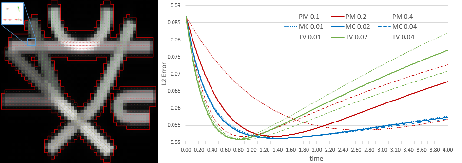
Figure 2: Quantitative comparison of denoising a fiber orientation density function (FODF) obtained by (CSD) [33] from a benchmark DW-MRI dataset [13].

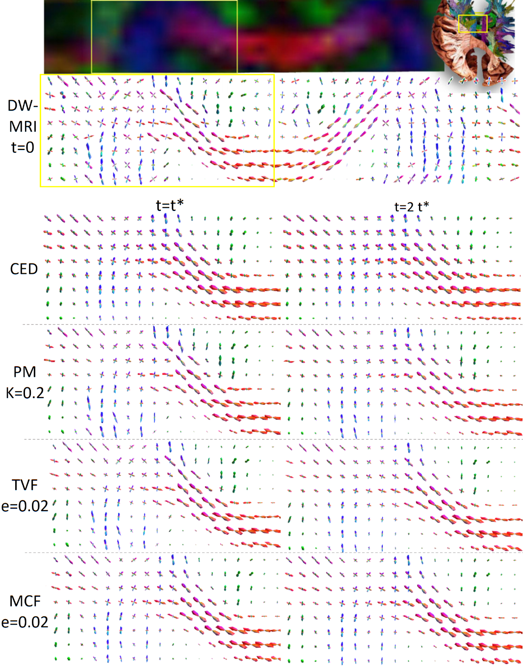
Figure 3: Qualitative comparison of denoising a FODF obtained by (CSD) [33] from a standard DW-MRI dataset (with $b=1000s/mm^{2}$ and $54$ gradient directions). For the CSD we used up to 8th order spherical harmonics, and the FODF is then spherically sampled on a tessellation of the icosahedron with 162 orientations.

For a qualitative comparison we applied TVF, MCF, PM diffusion and linear diffusion to a FODF field $U:\mathbb{M}\to\mathbb{R}^{+}$ obtained from a standard DW-MRI dataset (with $b=1000s/mm^{2}$, $54$ gradient directions) via constrained spherical deconvolution (CSD) [33]. See Fig. ​ 3, where for each method, we used the optimal parameter settings with the artificial data-set. We see that

• all methods perform well on the real datasets. Contextual alignment of the angular profiles better reflects the anatomical fiber bundles,

• MCF and TVF better preserve boundaries and angular sharpness,

• MCF better preserves the amplitude at crossings at longer times.

3.2 TVF & MCF on $\mathbb{R}^{2}\rtimes S^{1}$ for 2D Image Enhancement/Denoising

The initial condition for our TVF/MCF-PDE (13) is set by an orientation score [14] of image $f:\mathbb{R}^{2}\to\mathbb{R}$ given by $\mathcal{W}_{\psi}f(\mathbf{x},\mathbf{n})=(\psi_{\mathbf{n}}\star f)(\mathbf{x})$ where $\star$ denotes correlation and $\psi_{\mathbf{n}}$ is the rotated wavelet aligned with $\mathbf{n}\in S^{1}$. For $\psi$ we use a cake-wavelet [14, ch:4.6] $\psi$ with standard settings [25]. Then we compute:

$$f\mapsto\mathcal{W}_{\psi}f\mapsto\Phi_{t}(\mathcal{W}_{\psi}f)(\cdot,\cdot)\mapsto f_{t}^{a}(\cdot):=\int_{S^{1}}\Phi_{t}^{a}(\mathcal{W}_{\psi}f)(\cdot,\mathbf{n})\,{\rm d}\mu_{S^{1}}(\mathbf{n}).$$ (16)

for $t\geq 0$. Here $U\mapsto W(\cdot,t)=\Phi_{t}(U)$ denotes the flow operator on $\mathbb{M}$ (13), but then the PDE in (13) is re-expressed in the locally adaptive frame (LAD) $\{\mathcal{B}_{i}\}_{i=1}^{3}$ obtained by the method in [21, 17, 25]. The PDE then becomes
$\frac{\partial\tilde{W}}{\partial t}=(\|\nabla_{0}\tilde{W}\|^{2}_{0}+\varepsilon^{2})^{\frac{a}{2}}\sum\limits_{i=1}^{3}\tilde{D}_{ii}\;\mathcal{B}_{i}\circ(\|\nabla_{0}\tilde{W}\|^{2}_{0}+\varepsilon^{2})^{-\frac{1}{2}}\mathcal{B}_{i}\tilde{W},\qquad a\in\{0,1\}$,
with $\tilde{D}_{11}=1$, $\tilde{D}_{22}=\tilde{D}_{33}$ as in CED-OS [21, eq.72]. By the invertibility of the orientation score one has $f=f_{0}^{a}$ so all flows depart from the original image.

For $a=0$ we call $f\mapsto f_{t}^{a}$ given by (16) a ‘TVF-OS flow’, for $a=1$ we call it a ‘MCF-OS flow’. In Fig.​ 4 we show how errors progress with $t\geq 0$. We see that inclusion of LAD is beneficial on the real image. In Fig. 5 we give a qualitative comparison to CED-OS [21]. Lines and plateaus are best preserved by TVF-OS.

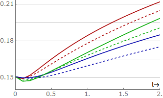
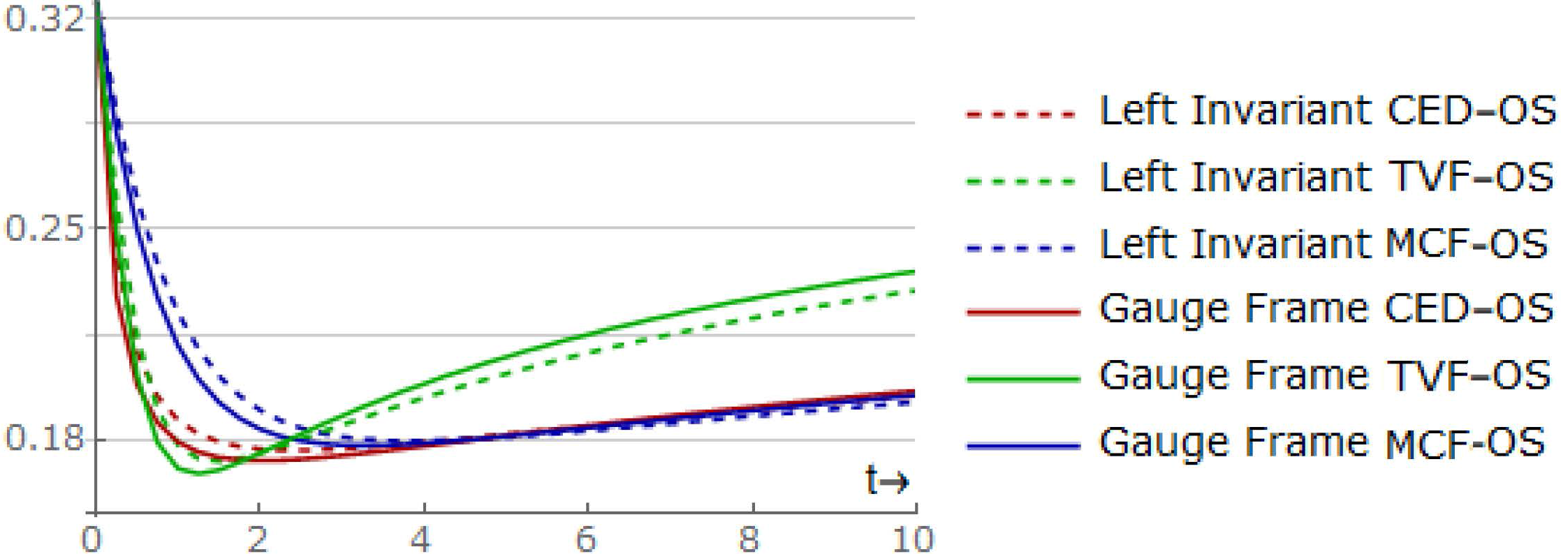
Figure 4: Relative $\mathbb{L}_{1}$ errors of the spirals test image (left) and the collagen image (right) for the CED-OS, MCF-OS and TVF-OS methods.

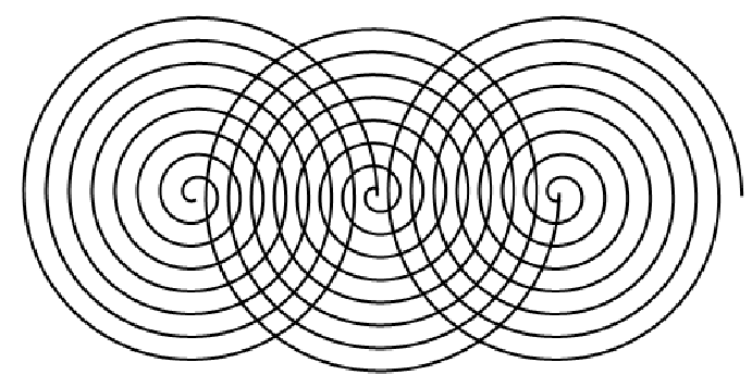
(a)

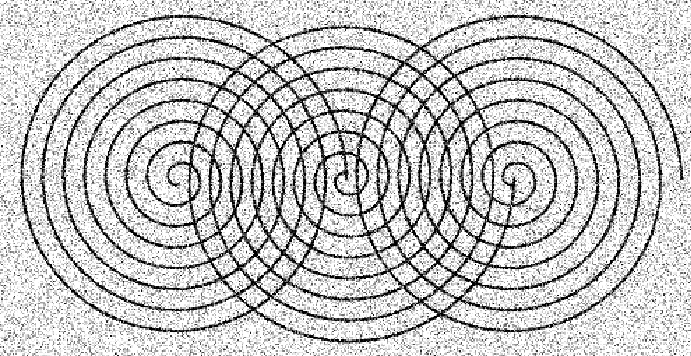
(b)

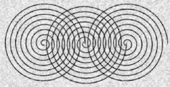
(c)

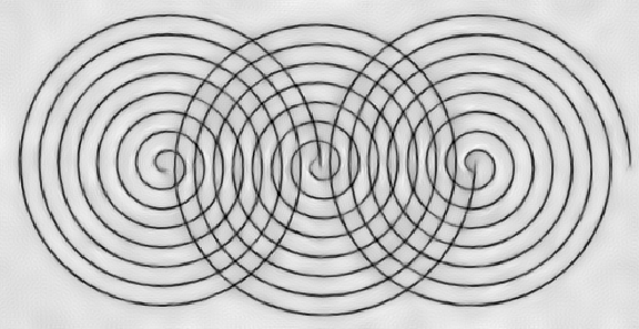
(d)

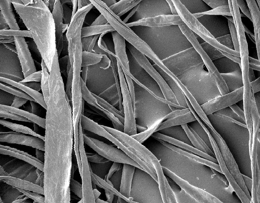
(e)

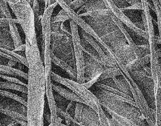
(f)

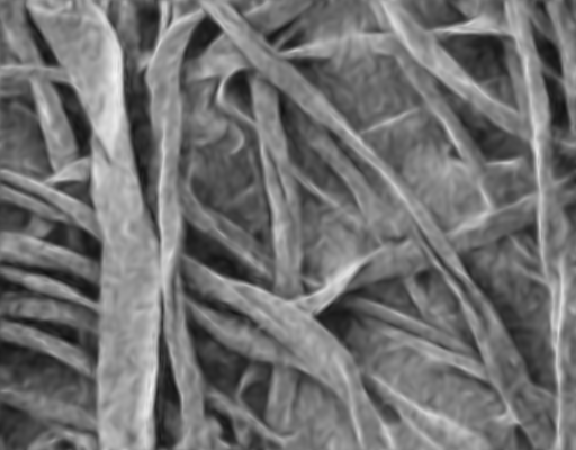
(g)

(h)

Figure 5: From left to right; original image; noisy input image $f$, CED-OS output image [21], TVF-OS output image $f_{t}^{0}$. We have set $D_{A}=0.01$, $D_{S}=1$, and took $t=10\cdot t^{*}$ for the spirals image and $t=2\cdot t^{*}$ for the collagen image where $t^{*}$ minimizes the relative $\mathbb{L}_{1}$-error to stress different qualitative behavior.

4 Conclusion

We have proposed a PDE system on the homogeneous space $\mathbb{M}=\mathbb{R}^{d}\rtimes S^{d-1}$ of positions and orientations, for crossing-preserving denoising and enhancement of (lifted) images containing both complex elongated structures and plateaus.

It includes TVF, MCF and diffusion flows as special cases, and includes (sub-)Riemannian geometry. Thereby we generalized recent related works by Citti et al. [9] and Chambolle & Pock [8] from 2D to 3D using a different numerical scheme with new convergence results (Theorem 2.1) and stability bounds. We used the divergence and intrinsic gradient on a (sub)-Riemannian manifold above $\mathbb{M}$ for a formal weak-formulation of total variation flows, which simplifies if the lifted images are differentiable (Lemma 1).

Compared to previous nonlinear crossing-preserving diffusion methods on $\mathbb{M}$, we showed improvements (Fig. 4,5) over CED-OS methods [21] (for $d=2$) and improvements over contextual fiber enhancement methods in DW-MRI processing (for $d=3$) [12, 15] on real medical image data. We observe that crossings and boundaries (of bundles and plateaus) are better preserved over time. We support this quantitatively by a denoising experiment on a benchmark DW-MRI dataset, where MCF performs better than TVF and both perform better than Perona-Malik diffusions, in view of error reduction and stability.

Appendix A: Proof of Theorem 2.

A functional $\Phi:H\to(-\infty,\infty]$ is said to be $\lambda$-convex for some $\lambda\in\mathbb{R}$ if

$$u\mapsto\Phi(u)-\frac{\lambda}{2}\|u\|^{2}$$

is convex. In that case, the functional

$$u\mapsto\Phi(u)-\frac{\lambda}{2}\|u-v\|^{2}$$

is convex as well, for arbitrary $v\in H$, because the latter functional deviates from the first by an affine functional.

We first prove a stability estimate for the minimization of $1/\tau$-convex functionals.

Lemma 2

Let $\tau>0$. If a functional $\Phi:H\to(-\infty,\infty]$ on $H$ is $1/\tau$-convex, and $u^{*}$ is its unique minimizer, then for all $u\in H$,

$$\frac{1}{2\tau}\|u-u^{*}\|^{2}\leq\Phi(u)-\Phi(u^{*}).$$

Proof

The functional $\Psi:H\to(-\infty,\infty]$ given by

$$\Psi(u):=\Phi(u)-\Phi(u^{*})-\frac{1}{2\tau}\|u-u^{*}\|^{2}$$

is convex. It is sufficient to show that $\Psi$ is nonnegative. If it were not, there would exist a $v\in H$ such that $\Psi(v)<0$. We will show that then, for $t$ small enough, $\Phi(tv+(1-t)u^{*})<\Phi(u^{*})$, contradicting that $u^{*}$ is a minimizer. We first have by definition that, for $t\in(0,1)$,

$$\begin{split}\Phi(tv+(1-t)u^{*})&-\Phi(u^{*})-\frac{t^{2}}{2\tau}\|v-u^{*}\|^{2}\\ &=\Psi(tv+(1-t)u^{*}).\end{split}$$

By the convexity of $\Psi$,

$$\begin{split}\Psi(tv+(1-t)u^{*})&\leq t\Psi(v)+(1-t)\Psi(u^{*})\\ &=t\Psi(v).\end{split}$$

Combining the two inequalities, we find

$$\Phi(tv+(1-t)u^{*})-\Phi(u^{*})\leq t\Psi(v)+O(t^{2}),$$

so that indeed, for $t$ small enough, $\Phi(tv+(1-t)u^{*})<\Phi(u^{*})$, leading to the announced contradiction.

Therefore, $\Psi$ is nonnegative, which means that

$$\frac{1}{2\tau}\|u-u^{*}\|^{2}\leq\Phi(u)-\Phi(u^{*})$$

for all $u\in H$.

For a proper (i.e. not everywhere equal to $\infty$), lower semicontinuous, convex functional $F$, and $\tau>0$, define the operator $J_{\tau}^{F}:H\to H$ by

$$J_{\tau}^{F}[u_{0}]:=\mathrm{argmin}_{u\in H}\left(\frac{1}{2\tau}\|u-u_{0}\|^{2}+F(u)\right).$$

Proposition 1

Let $F,G:H\to[0,\infty]$ be two non-negative, proper, lower semicontinuous, convex functionals on a Hilbert space $H$, such that for all $u\in H$,

$$F(u)-\delta\leq G(u)\leq F(u)+\delta.$$ (17)

Let $u_{0},v_{0}\in H$, such that

$$|\partial F|(u_{0})\leq L\quad\text{ and }\quad|\partial G|(v_{0})\leq L.$$ (18)

Then, we have the following estimate for the gradient flow $u:[0,\infty)\to H$ of $F$ starting at $u_{0}$ and the gradient flow $v:[0,\infty)\to H$ of $G$ starting at $v_{0}$:

$$\|u(t)-v(t)\|\leq\begin{cases}4\sqrt{\delta t}+\|u_{0}-v_{0}\|&\text{for }0\leq t\leq\frac{\delta}{L^{2}}\\ 8\sqrt[3]{L\delta t^{2}}+\|u_{0}-v_{0}\|&\text{for }t>\frac{\delta}{L^{2}}.\end{cases}$$

The idea is that the stability estimate in Lemma 2 will allow us to conclude that $J_{\tau}^{F}[u_{0}]$ and $J_{\tau}^{G}[v_{0}]$ are close when $u_{0}$ and $v_{0}$ are close. By iterating the operators $J_{\tau}^{F}$ and $J_{\tau}^{G}$, we approximate the gradient flows of $F$ and $G$ respectively, and from the slope estimate (17) we will derive that this approximation is uniform. This will allow us to derive bounds for the gradient flows from the bounds for $J_{\tau}^{F}$ and $J_{\tau}^{G}$.

Proof

Let $\tau>0$ and let $u_{1}^{F}:=J^{F}_{\tau}[u_{0}]$ and $v_{1}^{G}:=J^{G}_{\tau}[v_{0}]$. Set also $v_{1}^{F}:=J^{F}_{\tau}[v_{0}]$ and $u_{1}^{G}:=J^{G}_{\tau}[u_{0}]$. Then, using the definition of $v_{1}^{F}$ in the second inequality below, we find

$$\begin{split}\frac{1}{2\tau}&\|v_{1}^{F}-v_{0}\|^{2}+G(v_{1}^{F})\\ &\overset{(\ref{eq:two-sided-bound})}{\leq}\frac{1}{2\tau}\|v_{1}^{F}-v_{0}\|^{2}+F(v_{1}^{F})+\delta\\ &\leq\frac{1}{2\tau}\|v_{1}^{G}-v_{0}\|^{2}+F(v_{1}^{G})+\delta\\ &\overset{(\ref{eq:two-sided-bound})}{\leq}\frac{1}{2\tau}\|v_{1}^{G}-v_{0}\|^{2}+G(v_{1}^{G})+2\delta.\end{split}$$

Because the functional

$$v\mapsto\frac{1}{2\tau}\|v-v_{0}\|^{2}+G(v)$$

is $1/\tau$-convex, it follows by Lemma 2 that

$$\frac{1}{2\tau}\|v_{1}^{F}-v_{1}^{G}\|^{2}\leq 2\delta.$$

Now we use that $J_{\tau}^{F}$ is non-expansive [1, Eq. (4.0.2)], so

$$\|u_{1}^{F}-v_{1}^{F}\|=\|J_{\tau}^{F}(u_{0})-J_{\tau}^{F}(v_{0})\|\leq\|u_{0}-v_{0}\|.$$

We conclude that

$$\|u_{1}^{F}-v_{1}^{G}\|\leq\|u_{0}-v_{0}\|+2\sqrt{\delta\tau}.$$

By iterating this estimate, we derive

$$\|(J_{\tau}^{F})^{n}[u_{0}]-(J_{\tau}^{G})^{n}[v_{0}]\|\leq\|u_{0}-v_{0}\|+2n\sqrt{\delta\tau}.$$ (19)

The a priori estimate [1, Theorem 4.0.4, (v)] yields that the gradient flows $u$ and $v$ of $F$ and $G$ respectively are approximated well by $(J_{t/n}^{F})^{n}[u_{0}]$ and $(J_{t/n}^{G})^{n}[v_{0}]$. More precisely, for $t>0$ and $n>0$, the a priori estimate gives

$$\left\|u(t)-(J_{\tau}^{F})^{n}\right\|\leq\frac{Lt}{\sqrt{2}n}\quad\text{ and }\quad\left\|v(t)-(J_{\tau}^{G})^{n}\right\|\leq\frac{Lt}{\sqrt{2}n}.$$

By these a priori estimates and the estimate for the discrete flows (19), we see that

$$\begin{split}\|u(t)-v(t)\|&\leq\|u(t)-(J_{t/n}^{F})^{n}[u_{0}]\|+\|v(t)-(J_{t/n}^{F})^{n}[v_{0}]\|\\ &\qquad+\|(J_{t/n}^{F})^{n}[u_{0}]-(J_{t/n}^{G})^{n}[v_{0}]\|\\ &\leq\sqrt{2}L\frac{t}{n}+2n\sqrt{\frac{\delta t}{n}}+\|u_{0}-v_{0}\|.\end{split}$$

To derive the final estimates, we need to make good choices for $n$. If $0\leq t\leq\delta/L^{2}$, we take $n=1$ and obtain

$$\begin{split}\|u(t)-v(t)\|&\leq\sqrt{2}Lt+2\sqrt{\delta t}+\|u_{0}-v_{0}\|\\ &\leq 4\sqrt{\delta t}+\|u_{0}-v_{0}\|.\end{split}$$

If $t>\delta/L^{2}$, we choose $n=\lceil L^{2/3}(t/\delta)^{1/3}\rceil$, which is larger than or equal to $2$. In that case,

$$n/2\leq n-1<L^{2/3}(t/\delta)^{1/3}\leq n.$$

We then obtain

$$\|u(t)-v(t)\|\leq 8L^{1/3}\delta^{1/3}t^{2/3}+\|u_{0}-v_{0}\|.$$

We now know that the gradient flows of $F$ and $G$ are close when the slopes $|\partial F|(u_{0})$ and $|\partial G|(v_{0})$ are bounded. This assumption can be rather stringent. We will relax it, and merely require that $F(u_{0})$ and $G(v_{0})$ are bounded by some constant $E>0$, in exchange for a bound between gradient flows that is slightly worse. Our approach will be to run the gradient flow for a small time $s$ from $u_{0}$ and $v_{0}$, and use the regularizing property of the gradient flow to conclude a slope bound. On the other hand, if $s$ is small, $u(s)$ and $v(s)$ will be close to $u_{0}$ and $v_{0}$. We will then choose $s$ (almost) optimally to derive a bound between the gradient flows.

Theorem 4.1

Let $F:H\to[0,\infty]$ and $G:H\to[0,\infty]$ be two proper, lower semicontinuous, convex functionals on a Hilbert space $H$, such that

$$F(u)-\delta\leq G(u)\leq F(u)+\delta$$

for all $u\in H$. Let $u_{0},v_{0}\in H$ be such that $F(u_{0})\leq E$ and $G(v_{0})\leq E$ and $\|u_{0}-u^{*}\|\leq M$ and $\|v_{0}-v^{*}\|\leq M$, for some constants $E,M>0$, where $u^{*}$ and $v^{*}$ minimize $F$ and $G$ respectively. The gradient flow $u:[0,\infty)\to H$ of $F$ starting at $u_{0}$, and the gradient flow $v:[0,\infty)\to H$ of $G$ starting at $v_{0}$ satisfy

$$\|u(t)-v(t)\|\leq 16(ME\delta t^{2})^{1/5}+\|u_{0}-v_{0}\|$$

for all $0\leq t<E^{6}M^{6}/\delta^{9}$.

Proof

By the Evolution Variational Inequality [1, Theorem 4.0.4, (iii)], we know that for all $s>0$

$$\|u(s)-u_{0}\|\leq\sqrt{2sF(u_{0})}$$ (20a)

and

$$\|v(s)-v_{0}\|\leq\sqrt{2sG(v_{0})}.$$ (20b)

By the regularizing property [1, Theorem 4.0.4, (ii)],

$$|\partial F|(u(s))\leq\frac{1}{s}\|u_{0}-u^{*}\|\leq\frac{M}{s}$$ (21a)

and

$$|\partial G|(v(s))\leq\frac{1}{s}\|v_{0}-v^{*}\|\leq\frac{M}{s}$$ (21b)

where $u^{*}$ minimizes $F$ and $v^{*}$ minimizes $G$.

Because the gradient flow is a non-expansive semigroup [1, Theorem 4.0.4, (iv)], we get

$$\begin{split}\|u(t)-v(t)\|&\leq\|u(t+s)-v(t+s)\|+\|u(t+s)-u(t)\|+\|v(t+s)-v(t)\|\\ &\leq\|u(t+s)-v(t+s)\|+\|u(s)-u_{0}\|+\|v(s)-v_{0}\|.\end{split}$$

Now assume $t<E^{6}M^{6}/\delta^{9}$. We will want to choose $s$ (almost) optimally, depending on $t$. We choose

$$s=\frac{M^{2/5}\delta^{2/5}t^{4/5}}{E^{3/5}}$$

and note that with $L:=M/s$, we have

$$t\geq\frac{\delta}{L^{2}}.$$

By the slope estimates (21) we can apply Proposition 1 to the gradient flows starting at $u(s)$ and $v(s)$, to get

$$\begin{split}\|u(t)-v(t)\|&\leq 8M^{1/3}s^{-1/3}\delta^{1/3}t^{2/3}+\|u(s)-v(s)\|+\|u(s)-u_{0}\|+\|v(s)-v_{0}\|\\ &\leq 8M^{1/3}s^{-1/3}\delta^{1/3}t^{2/3}+2\|u(s)-u_{0}\|+2\|v(s)-v_{0}\|+\|u_{0}-v_{0}\|\\ &\overset{(\ref{eq:close-to-initial})}{\leq}8M^{1/3}s^{-1/3}\delta^{1/3}t^{2/3}+\sqrt{32sE}+\|u_{0}-v_{0}\|\\ &=16M^{1/5}\delta^{1/5}t^{2/5}E^{1/5}+\|u_{0}-v_{0}\|.\end{split}$$

References

- [1] Ambrosio, L., Gigli, N., Savaré, G.: Gradient flows in metric spaces and in the space of probability measures. Bikhäuser (2005)
- [2] Baspinar, E., Citti, G., Sarti, A.: A geometric model of multi-scale orientation preference maps via gabor functions. JMIV 60(6), 900–912 (2018)
- [3] Baspinar, E.: Minimal Surfaces in Sub-Riemannian Structures and Functional Geometry of the Visual Cortex. Ph.D. thesis, University of Bologna (2018)
- [4] Bekkers, E.: Retinal Image Analysis using Sub-Riemannian Geometry in . Ph.D. thesis, TU/e Eindhoven (2017)
- [5] Bekkers, E., Duits, R., Mashatkov, A., Sanguinetti, G.: A PDE approach to data-driven sub-Riemannian geodesics in . SIIMS 8(4), 2740–2770 (2015)
- [6] Boscain, U., Chertovskih, R., Gauthier, J.P., Prandi, D., Remizov, A.: Highly corrupted image inpainting by hypoelliptic diffusion. JMIV 60(8), 1231–1245 (2018)
- [7] Brézis, H.: Operateurs maximeaux monotones et semi-gropes de contractions dans les espaces de Hilbert, vol. 50. North-Holland Publishing Co. (1973)
- [8] Chambolle, A., Pock, T.: Total roto-translation variation. Arxiv:17009.099532v2 pp. 1–47 (july 2018)
- [9] Citti, G., Franceschiello, B., Sanguinetti, G., Sarti, A.: Sub-riemannian mean curvature flow for image processing. SIIMS 9(1), 212–237 (2016)
- [10] Citti, G., Sarti, A.: A cortical based model of perceptional completion in the roto-translation space. JMIV 24(3), 307–326 (2006)
- [11] Cohen, E., Deffieux, T., Demené, C., Cohen, L., Tanter, M.: 3d vessel extraction in the rat brain from ultrasensitive doppler images. Computer Methods in Biomechanics and Biomedical Engineering. LNB pp. 81–91 (2018)
- [12] Creusen, E.J. & Duits, R., Florack, L., Vilanova, A.: Numerical schemes for linear and non-linear enhancement of DW-MRI. NM-TMA 6(3), 138–168 (2013)
- [13] Daducci, A., Caruyer, E., Descoteaux, M., Thiran, J.P.: HARDI Reconstruction Challenge (2013), published at IEEE ISBI 2013
- [14] Duits, R.: Perceptual organization in image analysis. Ph.D. thesis, TU/e (2005)
- [15] Duits, R., Creusen, E., Ghosh, A., Dela Haije, T.: Morphological and linear scale spaces for fiber enhancement in DW-MRI. JMIV 46(3), 326–368 (2013)
- [16] Duits, R., Franken, E.M.: Left invariant parabolic evolution equations on and contour enhancement via invertible orientation scores, part I: Linear left-invariant diffusion equations on . QAM-AMS 68, 255–292 (2010)
- [17] Duits, R., Janssen, M., Hannink, J., Sanguinetti, G.: Locally adaptive frames in the roto-translation group and their applications in medical image processing. JMIV 56(3), 367–402 (2016)
- [18] Duits, R., Meesters, S., Mirebeau, J., Portegies, J.: Optimal paths for variants of the 2D and 3D Reeds-Shepp car with applications in image analysis. JMIV 60, 816–848 (2018)
- [19] Evans, L.C., Spruck, J.: Motion of level sets by mean curvature. I. J. Differential Geom. 33(3), 635–681 (1991)
- [20] Felsberg, M., Forssen, P.E., Scharr, H.: Channel smoothing: Efficient robust smoothing of low-level signal features. IEEE PAMI pp. 209–222 (2006)
- [21] Franken, E.M., Duits, R.: Crossing preserving coherence-enhancing diffusion on invertible orientation scores. IJCV 85(3), 253–278 (2009)
- [22] Giga, Y., Sato, M.H.: Generalized interface evolution with the Neumann boundary condition. Proc. Japan Acad. Ser. A Math. Sci. 67(8), 263–266 (1991)
- [23] G.Sapiro: Geometric Partial Differential Equations & Image Analysis. CUP (2006)
- [24] Janssen, M.H.J., Janssen, A.J.E.M., Bekkers, E.J., Bescós, J.O., Duits, R.: Processing of invertible orientation scores of 3d images. JMIV 60(9), 1427–1458 (2018)
- [25] Martin, F., Bekkers, E., Duits, R.: Lie analysis package:. www.lieanalysis.nl/ (2017)
- [26] Meesters, S., et al.: Stability metrics for optic radiation tractography: Towards damage prediction after resective surgery. Journal of Neuroscience Methods (2017)
- [27] Portegies, J.M., Duits, R.: New exact and numerical solutions of the (convection-) diffusion kernels on SE(3). DGA 53, 182–219 (2017)
- [28] Portegies, J.M., Fick, R., Sanguinetti, G.R., Meesters, S.P.L., Girard, G., Duits, R.: Improving Fiber Alignment in HARDI by Combining Contextual PDE Flow with Constrained Spherical Deconvolution. PLoS ONE 10(10) (2015)
- [29] Portegies, J.: PDEs on the Lie Group SE(3) and their Applications in Diffusion-Weighted MRI. Ph.D. thesis, Dep. Math. TU/e (2018)
- [30] Reisert, M., Burkhardt, H.: Efficient tensor voting with 3d tensorial harmonics. In: CVPRW ’08. IEEE Conf. pp. 1 –7 (2008)
- [31] Sato, M.H.: Interface evolution with Neumann boundary condition. Adv. Math. Sci. Appl. 4(1), 249–264 (1994)
- [32] Schmidt, M., Weickert, J.: Morphological counterparts of linear shift-invariant scale-spaces. Journal of Mathematical Imaging and Vision 56(2), 352–366 (2016)
- [33] Tournier, J.D., Calamante, F., Connelly, A.: MRtrix: Diffusion tractography in crossing fiber regions. Int. J. Imag. Syst. Tech. 22(1), 53–66 (2012)
- [34] Vogt, T., Lellmann, J.: Measure-valued variational models with applications to diffusion-weighted imaging. JMIV 60(9), 1482–1502 (2018)
- [35] Weickert, J.A.: Coherence-enhancing diffusion filtering 31(2/3), 111–127 (1999)