Stochastic Local Interaction Model with Sparse Precision Matrix for Space-Time Interpolation

Abstract

The application of geostatistical and machine learning methods based on Gaussian processes to big space-time data is beset by the requirement for storing and numerically inverting large and dense covariance matrices. Computationally efficient representations of space-time correlations can be constructed using local models of conditional dependence which can reduce the computational load. We formulate a stochastic local interaction model for regular and scattered space-time data that incorporates interactions within controlled space-time neighborhoods. The strength of the interaction and the size of the neighborhood are defined by means of kernel functions and adaptive local bandwidths. Compactly supported kernels lead to finite-size local neighborhoods and consequently to sparse precision matrices that admit explicit expression. Hence, the stochastic local interaction model’s requirements for storage are modest and the costly covariance matrix inversion is not needed. We also derive a semi-explicit prediction equation and express the conditional variance of the prediction in terms of the diagonal of the precision matrix. For data on regular space-time lattices, the stochastic local interaction model is equivalent to a Gaussian Markov Random Field.

1 Introduction

Space-time (ST) data are becoming available in overwhelming volumes and diverse forms due to the continuing growth of remote-sensing capabilities, the deployment of low-cost, ground-based sensor networks, as well as the increasing usage of sensors based on unmanned aerial vehicles, and crowdsourcing [1]. The ongoing data explosion has an impact in various fields of science and engineering. The modeling and processing of massive ST datasets poses conceptual, methodological, and technical challenges. Sufficiently flexible and computationally powerful solutions are not widely available to date, because most existing methods are not designed for global, high-volume, hyper-dimensional, heterogeneous and uncertain ST data. For example, classical geostatistical and machine learning methods [2, 3] are limited by the cubic dependence of the computational time on data size, which is prohibitive even for large purely spatial data.

The modeling and processing of ST data require more advanced methods and computational resources than those that are adequate for purely spatial data. For example, theories that simply extend spatial statistics by adding a separable time dimension are often inadequate for capturing realistic correlations and for analyzing massive ST data [4, 5]. Various methods have been proposed for developing non-separable covariance models [6, 7, 8]. Current methods, whether they are based on geostatistics [2], spatio-temporal statistics [9, 5], or machine learning [3] face serious scalability problems. A prevailing obstacle in the processing chain is the computationally demanding iterated inversion of large covariance (Gram) matrices [3, 10]. Hence, classical methods executed on standard desktop computers are limited to datasets with size $N\sim\mathcal{O}(10^{3})-\mathcal{O}(10^{4})$. Various approaches for alleviating the dimensionality problem (covariance tapering, composite likelihood, low-rank computations, stochastic partial differential equation representation, etc.) have been proposed and developed [10].

In the case of continuum random fields, Gaussian field theories of statistical physics provide models with local structure which is derived from the derivatives of the field [11]. Gaussian Markov random fields (GMRFs) also share the local property, since they are defined in terms of interactions that involve local neighborhoods [12]. Stochastic local interaction (SLI) models are inspired from GMRFs and Gaussian field theory. They are based on the idea that correlations are generated by interactions between neighboring sites and times. The interactions are incorporated in a precision matrix with simple parametric dependence.

We present a theoretical framework for the analysis of ST data that is based on stochastic local interaction (SLI) models [13, 14]. This formulation is useful for filling gaps by interpolation in ST datasets of environmental importance. For example, gaps in records of meteorological variables need to be reconstructed for the evaluation of renewable energy potential at candidate sites [15], while ground-based rainfall gauge networks often have missing data [16]. The main idea in SLI is that the ST correlations are determined by means of sparse precision matrices that only involve couplings between near neighbors (in the ST domain). In contrast with GMRF models that are typically defined on regular lattice data and field theories which are defined on continuum spaces, the SLI framework is suitable for direct application to scattered data and stochastic graph processes. However, it is also applicable to data on regular space-time lattices.

The remainder of this manuscript is structured as follows: In Section 2 we define the ST-SLI model and discuss its properties. In Section 3 we formulate ST prediction based on the SLI model, and in Section 4 we discuss parameter estimation from ST data. Following the theoretical formulation, Section 5 presents an application of the SLI method to three datasets which involve simulated ST data, reanalysis temperature data, and atmospheric ozone measurements. Finally, we present our conclusions and a brief discussion in Section 6.

2 ST Model based on Stochastic Local Interactions

A space-time scalar random field (STRF) $X({\bf s},t;\omega)\in\mathbb{R}$ where ${\bf s},t\in\mathbb{R}^{d}\times\mathbb{R}$ and $\omega\in\Omega$ is defined as a mapping from the probability space $(\Omega,A,P)$ into the space of real numbers $\mathbb{R}$. For each ST coordinate $({\bf s},t)$, $X({\bf s},t;\omega)$ is a measurable function of $\omega$, where $\omega$ is the state index [4]. The states (realizations) of the random field $X({\bf s},t;\omega)$ are real-valued functions $x({\bf s},t)$ obtained for a specific $\omega$. In the following, the state index $\omega$ is dropped to simplify notation.

We focus on partially sampled realizations $\mathbf{x}=\left(x_{1},\ldots,x_{N}\right)^{\top}$ of the random field, where $N\in\mathbb{N}$ is the sample size. The vector $\mathbf{x}$ comprises the field values at the ST point set $\mathbb{S}=\{({\bf s}_{1},t_{1}),\ldots,({\bf s}_{N},t_{N})\}$. The point set is assumed to be quite general; it may represent a time sequence of lattice sites, randomly scattered points in space and time, or a collection of time series at random locations in space.

2.1 Energy of the exponential joint density

The SLI model is based on a joint pdf defined by the Boltzmann-Gibbs exponential distribution

$$f_{{\rm x}}(\mathbf{x};{\bm{\theta}})=\frac{\mathrm{e}^{-\mathcal{H}(\mathbf{x};{\bm{\theta}})}}{Z({\bm{\theta}})},$$ (1)

where $\mathcal{H}(\cdot;\cdot)$ is an energy function that represents the “cost” of a specific configuration, ${\bm{\theta}}$ is a vector of model parameters, and $Z({\bm{\theta}})$ is the normalizing factor known as partition function.

The energy-based approach is commonly used in statistical physics [17, 11]. Its main advantage is that it expresses statistical dependence in terms of interactions between space locations and time instants which can be local, without recourse to the concept of the covariance matrix. Depending on the form of the interactions involved in the energy, both Gaussian and non-Gaussian probability density functions can be obtained. The most famous example of non-Gaussian dependence is the magnetic Ising model [18] which was introduced in spatial statistics by Besag [19]. While non-Gaussian models are definitely interesting, their Gaussian counterparts lead to explicit predictive expressions and uncertainty estimates based on the conditional variance. Hence, herein we focus on a Gaussian SLI model.

We assume that $\mathcal{H}(\mathbf{x};{\bm{\theta}})$ satisfies the following properties for any vector $\mathbf{x}\in\mathbb{R}^{N}$ and $N\in\mathbb{N}$:

1. Gaussianity: $\mathcal{H}(\mathbf{x};{\bm{\theta}})$ is a quadratic function of the data vector $\mathbf{x}$ that can be expressed as

   $$\mathcal{H}(\mathbf{x};{\bm{\theta}})=\frac{1}{2}(\mathbf{x}-\mathbf{{m_{{\rm x}}}})^{\top}\mathbf{J}({\bm{\theta}}^{\prime})(\mathbf{x}-\mathbf{{m_{{\rm x}}}}),$$ (2)

   where $\mathbf{{m_{{\rm x}}}}=\left({m_{{\rm x}}}_{;1},\ldots,{m_{{\rm x}}}_{;N}\right)^{\top}$ is a vector of mean (trend) values such that ${m_{{\rm x}}}_{;,i}=\mathcal{E}\left[{\,X({\bf s}_{i},t_{i})}\,\right]$, where $\mathcal{E}\left[{\,\cdot}\,\right]$ is the expectation operator. On the other hand, $\mathbf{J}({\bm{\theta}}^{\prime})$ is the $N\times N$ precision (or interaction) matrix. The latter depends on the parameter vector ${\bm{\theta}}^{\prime}={\bm{\theta}}\setminus\{b_{1},\ldots,b_{K}\}$ which excludes the trend coefficients. The vector $\mathbf{{m_{{\rm x}}}}$ incorporates both periodic and aperiodic trend components.

2. Positive-definiteness: $\mathcal{H}(\mathbf{x};{\bm{\theta}})>0$ for all $\mathbf{x}$ that are not identically equal to zero. This is equivalent to the precision matrix $\mathbf{J}({\bm{\theta}})$ being a positive-definite matrix.

3. Sparseness: $\mathbf{J}({\bm{\theta}}^{\prime})$ is a sparse matrix that incorporates the local interactions.

More specifically, we focus on the following SLI energy function which satisfies the properties of Gaussianity, positive-definiteness and sparseness:

$$\mathcal{H}(\mathbf{x};{\bm{\theta}})=\frac{1}{2\lambda}\left[\sum_{n=1}^{N}\frac{1}{N}(x_{n}-{m_{{\rm x}}}_{;n})^{2}+c_{1}\big{\langle}\left({x^{\prime}}_{n}-{x^{\prime}}_{k}\right)^{2}\big{\rangle}\right].$$ (3)

We assume that the mean is modeled by means of a trend function which can be expressed as ${m_{{\rm x}}}({\bf s},t)=\sum_{k=1}^{K}b_{k}f_{k}({\bf s},t)$ in terms of a suitable ST function basis $\{f_{k}({\bf s},t)\}_{k=1}^{K}$, where $\{b_{k}\}_{k=1}^{K}$ is a set of real-valued trend coefficients and $f_{k}:\mathbb{R}^{d}\times\mathbb{R}\to\mathbb{R}$, for $k=1,\ldots,K$.

The variables $x_{n},x_{k}$ stand for $x({\bf s}_{n},t_{n})$ and $x({\bf s}_{k},t_{k})$ respectively, where $n,k=1,\ldots N$ while ${x^{\prime}}_{n},{x^{\prime}}_{k}$ represent the residuals after the trend values are removed. The term $\big{\langle}\left({x^{\prime}}_{n}-{x^{\prime}}_{k}\right)^{2}\big{\rangle}$ represents a weighted average of the squared increments. However, instead of focusing on all $\mathcal{O}(N^{2})$ pairs, the average defined below selects only pairs within a local neighborhood around each point ${\bf s}_{n}$.

The SLI parameter vector ${\bm{\theta}}$ includes the trend coefficients $\{b_{k}\}_{k=1}^{K}$, the overall scale parameter $\lambda$ (which is proportional to the variance), and the increment coefficient $c_{1}$ (a dimensionless factor that multiplies the contribution from the squares of the increments). The vector ${\bm{\theta}}$ includes additional parameters that determine the local ST neighborhoods used in the average of the squared increments $\langle\cdot\rangle$. The average is defined in (4) below.

2.2 Kernel-based averaging

The weights in the average of the squared increments are defined by means of the Nadaraya-Watson equation [20, 21], i.e.,

$$\langle\left({x^{\prime}}_{n}-{x^{\prime}}_{k}\right)^{2}\rangle=\frac{\sum_{n=1}^{N}\sum_{k=1}^{N}w_{n,k}\left({x^{\prime}}_{n}-{x^{\prime}}_{k}\right)^{2}}{\sum_{n=1}^{N}\sum_{k=1}^{N}w_{n,k}}.$$ (4)

The coefficients $w_{n,k}$ are defined in terms of compactly supported ST kernel functions $K(\cdot,\cdot):\mathbb{R}^{q}\times\mathbb{R}^{q}\to\mathbb{R}$, where $q=d+1$ for an ST kernel, $q=d$ for a spatial kernel, and $q=1$ for a temporal kernel. Kernel functions are symmetric, real-valued functions; herein they are assumed to take values in the interval $[0,1]$ without loss of generality. Moreover, we will assume spatially homogeneous and temporally stationary kernel functions, i.e., $K({\bf s}_{1},{\bf s}_{2})=K({\bf s}_{1}-{\bf s}_{2})$, $K(t_{1},t_{2})=K(t_{1}-t_{2})$, and $K({\bf s}_{1},t_{1};{\bf s}_{2},t_{2})=K({\bf s}_{1}-{\bf s}_{2},t_{1}-t_{2})$. Furthermore, it will be assumed for simplicity that the kernel function depends only on the magnitude of the ST distance.

2.3 Definition of space-time distance

The space-time distance used in the kernel weights determines the structure of correlations that we impose in the space-time domain. Both separable and non-separable space-time metric distances are possible as discussed below.

Composite space-time distance: In this case the spatial and temporal coordinates are intertwined in the distance metric. For example, the differential of the space-time distance between two points using the Riemannian metric is

$$dq=\sqrt{\sum_{i=1}^{d+1}\sum_{j=1}^{d+1}g_{i,j}dz^{(i)}dz^{(j)}},$$ (5)

where $\{g_{i,j}\}_{i,j=1}^{d+1}$ are the elements of the metric tensor $\mathbf{g}$, $\{dz^{(i)}\}_{i=1}^{d}$, are the differentials of the spatial distance in the $d$ orthogonal directions, and $dz^{(d+1)}$ is the time differential [22, 23].

In the Euclidean case the metric tensor $\mathbf{g}$, is given by

$$g_{i,j}=\delta_{i,j}\left[1+\left(\alpha-1\right)\delta_{i,d+1}\right],\;i,j=1,\ldots,d+1,$$ (6)

where $\alpha$ is a parameter that controls the contribution of the time lag in the composite distance. The kernel coefficient based on the composite Euclidean metric can be expressed as

$$w_{n,k}=K\left(\frac{\sqrt{{\mathbf{r}}_{n,k}^{2}+\alpha^{2}\tau_{n,k}^{2}}}{h_{s,n}}\right).$$ (7)

In (7) ${\mathbf{r}}_{n,k}=\left({\bf s}_{n}-{\bf s}_{k}\right)$ is the spatial lag between the initial point ${\bf s}_{n}$ and the target point ${\bf s}_{k}$, and $h_{s,n}$ is the local spatial bandwidth at ${\bf s}_{n}$. In addition, $\tau_{n,k}=t_{n}-t_{k}$ is the temporal lag between the initial and target times. The space-time distance for the composite metric leads to ellipsoidal neighborhoods as shown in the schematic of Fig. 1(a). The temporal bandwidth in this case is $h_{t,n}=h_{s,n}/\alpha$.

Separable space-time distance: The coefficients $w_{n,k}$ for a separable space-time neighborhood are defined as

$$w_{n,k}=K\left(\frac{\|{\mathbf{r}}_{n,k}\|}{h_{s,n}}\right)\,K\left(\frac{|\tau_{n,k}|}{h_{t,n}}\right),\;n,k=1,\ldots,N.$$ (8)

In the weight equation (8) $h_{s,n}$ is the local spatial bandwidth at ${\bf s}_{n}$ and $h_{t,n}$ is the temporal bandwidth. The space-time distance for the separable space-time metric leads to cylindrical neighborhoods as shown in Fig. 1(b).

2.4 Definition of bandwidths

For each ST point $\{({\bf s}_{n},t_{n})\}_{n=1}^{N}$, the spatial bandwidth $h_{s,n}$ is determined from the geometry of the sampling network around the spatial point ${\bf s}_{n}$, while the temporal bandwidth $h_{t,n}$ is based on the time neighborhood around $t_{n}$. In general, this means that the number of bandwidth parameters scales linearly with the sampling size, leading to an under-determined estimation problem when the additional parameters are accounted for.

To simplify the bandwidth estimation we use a trick that reduces the dimensionality of the problem. We assign to each point a bandwidth which is proportional to the spatial distance $D_{n,[K_{s}]}(\mathbb{S})$ between this point and its $K_{s}$-nearest neighbor in the point set $\mathbb{S}$. Thus, it holds that $h_{s,n}=\mu_{s}\,D_{n,[K_{s}]}(\mathbb{S})$, where typically $K_{s}=2,3,4$, and $\mu_{s}>0$ is a dimensionless spatial bandwidth parameter to be estimated from the data.

In the case of the composite space-time distance the temporal bandwidths $h_{t,n}$ are determined from the $h_{s,n}$ and the additional parameter $\alpha$. For a separable ST distance metric, the temporal bandwidths are determined by means of $h_{t,n}=\mu_{t}\,\tilde{D}_{n,[K_{t}]}(\mathbb{S})$, where $K_{t}$ is the order of the temporal neighbor and $\mu_{t}>0$ is a dimensionless temporal bandwidth parameter. This definition of the temporal bandwidth in the case of uniform time step implies uniform bandwidths for all except the initial and final times, where the bandwidth is automatically increased to account for the missing left and right neighbors respectively.

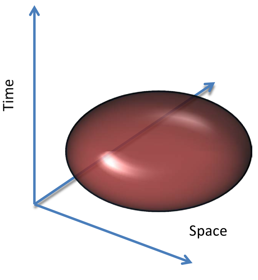
(a) Composite

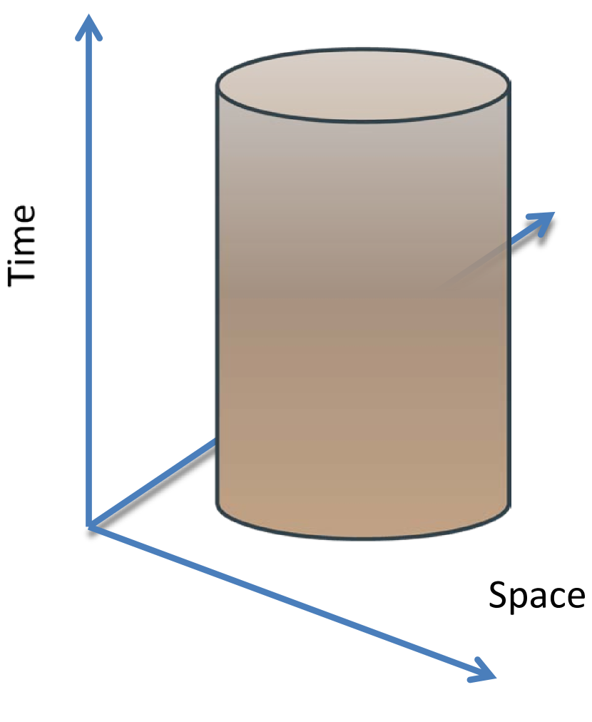
(b) Separable

Figure 1: Schematics of kernel-based neighborhoods for composite (left) and separable (right) space-time structures.

2.5 Properties of kernel weights

The kernel-average of the squared increments (4) can be expressed in terms of normalized weights $u_{n,k}$ as follows

$$\langle\left({x^{\prime}}_{n}-{x^{\prime}}_{k}\right)^{2}\,\rangle =\sum_{n=1}^{N}\sum_{k=1}^{N}u_{n,k}\left({x^{\prime}}_{n}-{x^{\prime}}_{k}\right)^{2},$$ (9a)

$$u_{n,k} =\frac{w_{n,k}}{\sum_{n=1}^{N}\sum_{k=1}^{N}w_{n,k}}.$$ (9b)

Normalization: The definition (9b) of the kernel weights implies that

$$\sum_{n=1}^{N}\sum_{k=1}^{N}u_{n,k}=1.$$

Asymmetry: The definition (9b) of the bandwidths is based on the local ST neighborhood. This implies that the spatial weights are in general asymmetric, i.e., $w_{n,k}\neq w_{k,n}$ if ${\bf s}_{n}\neq{\bf s}_{k}$, since the sampling density around the point ${\bf s}_{n}$ can be quite different than around the point ${\bf s}_{k}$.

Non-separability: The kernel weights $u_{n,k}$ are non-separable for both the composite and the separable ST distance metrics. In the first case this is obvious from the definition (7). In the second case, even though the $w_{n,k}$ are separable, the normalized weights $u_{n,k}$ are non-separable functions of space and time due to the kernel summation in the denominator of (4).

Robustness with respect to general distance metrics: Regardless of the distance metric used, the kernel-based weights $u_{n,k}$ are non-negative. This implies that the SLI energy function (3) is positive, and consequently the precision matrix is positive definite. Hence, general distance metrics, e.g., Manhattan (also known as city block and taxicab) distance, can be used in the SLI model.

In the following we develop the SLI formalism for a separable space-time metric structure.

2.6 Squared increments for separable space-time metric

In this section we formulate the average squared increments for separable space-time kernel functions using matrix operations.

First, we define the square kernel matrices $\mathbf{K}_{s}$ of dimension $N_{s}\times N_{s}$ and $\mathbf{K}_{t}$ of dimension $N_{t}\times N_{t}$ as follows

$$\mathbf{K}_{s}=\left[\begin{array}[]{cccc}K\left(\frac{\|{\mathbf{r}}_{1,1}\|}{h_{s,1}}\right)&\ldots&K\left(\frac{\|{\mathbf{r}}_{1,N_{s}}\|}{h_{s,1}}\right)\\ \vdots&\vdots&\vdots\\ K\left(\frac{\|{\mathbf{r}}_{N_{s},1}\|}{h_{s,N_{s}}}\right)&\ldots&K\left(\frac{\|{\mathbf{r}}_{N_{s},N_{s}}\|}{h_{s,N_{s}}}\right)\\ \end{array}\right],$$ (10a)

$$\mathbf{K}_{t}=\left[\begin{array}[]{cccc}K\left(\frac{\|\tau_{1,1}\|}{h_{t,1}}\right)&\ldots&K\left(\frac{\|\tau_{1,N_{t}}\|}{h_{t,1}}\right)\\ \vdots&\vdots&\vdots\\ K\left(\frac{\|\tau_{N_{t},1}\|}{h_{t,N_{t}}}\right)&\ldots&K\left(\frac{\|\tau_{N_{t},N_{t}}\|}{h_{t,N_{t}}}\right)\\ \end{array}\right].$$ (10b)

Then, the $N\times N$ matrix $\mathbf{W}$ of ST kernel weights is given by the following Kronecker product (denoted by $\otimes$):

$$\mathbf{W}=\mathbf{K}_{s}\otimes\mathbf{K}_{t}.$$ (10c)

For compactly supported kernel functions the matrix $\mathbf{W}$ given by (10c) is sparse.

The matrix $\mathbf{U}$ of the normalized kernel weights is then defined by means of

$$\mathbf{U}=\frac{\mathbf{W}}{\|\mathbf{W}\|_{1}},$$ (11a)

where the denominator $$\|\mathbf{W}\|_{1} L_{1} \mathbf{W}$$ represents the entry-wise norm of the matrix and is given by

$$\|\mathbf{W}\|_{1}=\sum_{k=1}^{N}\sum_{l=1}^{N}|W_{k,l}|.$$ (11b)

In terms of the above matrices, the average squared increment (9) is expressed as follows

$$\langle\left({x^{\prime}}_{n}-{x^{\prime}}_{k}\right)^{2}\rangle=\left\|\left[\left(\mathbf{x}^{\prime}\otimes\mathbf{1}\right)-\left(\mathbf{x}^{\prime}\otimes\mathbf{1}\right)^{\top}\right]\circ\mathbf{U}\circ\left[\left(\mathbf{x}^{\prime}\otimes\mathbf{1}\right)-\left(\mathbf{x}^{\prime}\otimes\mathbf{1}\right)^{\top}\right]\right\|_{1}$$ (12)

where $\mathbf{1}=(1,\ldots,1)^{\top}$ is the $N\times 1$ vector of ones, and $\circ$ denotes the Hadamard product, i.e., $\left[\mathbf{A}\circ\mathbf{B}\right]_{i,j}=A_{i,j}B_{i,j}$.

The computational complexity of the operations in (12) is $\mathcal{O}(N^{2})$, if the sparsity of the matrix $\mathbf{W}$ is not taken into account. However, the numerical complexity can be improved using sparse-matrix operations. We have implemented all the calculations which involve the precision matrix using sparse matrix functionality.

2.7 Precision matrix formulation

In light of the above definitions, the SLI energy function (3) involves the following parameter vector

$${\bm{\theta}}=\left(b_{1},\ldots,b_{K},\lambda,c_{1},\mu_{s},\mu_{t},K_{s},K_{t}\right)^{\top},$$ (13)

where $\{b_{k}\}_{k=1}^{K}$ are the coefficients of the trend model, $\lambda$ is the SLI scaling factor, $c_{1}$ is the square increment coefficient, $\mu_{s},\mu_{t}$ the dimensionless scaling factors used to determine the bandwidths, and $K_{s},K_{t}$ are the orders of spatial and temporal near neighbors respectively.

The SLI energy function (3) can be transformed into a quadratic energy functional, i.e., of the form of equation (2), by defining the precision matrix ${\mathbf{J}}({\bm{\theta}}^{\prime})$ as follows

$${\mathbf{J}}({\bm{\theta}}^{\prime})=\frac{1}{\lambda} \,\left\{\frac{{\bf I}_{N}}{N}+c_{1}\,{\mathbf{J}}_{1}({{\mathbf{h}}};{\bm{\theta}}^{\prime\prime})\right\},$$ (14)

where ${\bf I}_{N}$ is the $N\times N$ identity matrix: $[{\bf I}_{N}]_{i,j}=1$ if $i=j$ and $[{\bf I}_{N}]_{i,j}=0$ otherwise. The precision matrix ${\mathbf{J}}({\bm{\theta}}^{\prime})$ involves the parameter vector ${\bm{\theta}}^{\prime}=\left(\lambda,c_{1},\mu_{s},\mu_{t},K_{s},K_{t}\right)^{\top}$. The matrix ${\mathbf{J}}_{1}({{\mathbf{h}}};{\bm{\theta}}^{\prime\prime})$ is derived from the average squared increments (9), and ${\bm{\theta}}^{\prime\prime}=\left(\mu_{s},\mu_{t},K_{s},K_{t}\right)^{\top}$ is the parameter vector which determines the kernel bandwidths. The precision matrix is thus expressed in terms of the normalized weights $u_{n,k}$ according to

$$[{\mathbf{J}}_{1}({{\mathbf{h}}};{\bm{\theta}}^{\prime\prime})]_{n,k} =-u_{n,k}-u_{k,n}+[{\bf I}_{N}]_{n,k}\,\sum_{l=1}^{N}\left(u_{n,l}+u_{l,n}\right),$$ (15)

where the normalized weights $u_{n,k}$ are given by (9b). Hence, the precision matrix is determined by the sampling pattern, the kernel functions, and the bandwidths.

3 ST Prediction

In this section we consider ST prediction by means of the SLI model at the set of space time points $\mathbb{G}=\{{\mathbf{\tilde{s}}}_{p}\}_{p=1}^{P}$, where ${\mathbf{\tilde{s}}}_{p}=(\tilde{{\bf s}}_{p},\tilde{t}_{p})$, assuming that the model parameters are known. It is further assumed that the sets $\mathbb{S}$ and $\mathbb{G}$ are disjoint. For example, the set $\mathbb{G}$ could comprise all the nodes of a regular map grid at a time instant $t_{p}$ for which measurements are not available. Alternatively, $\mathbb{G}$ could comprise all the nodes of an irregular spatial sampling network at a time instant with no measurements.

3.1 SLI energy function including prediction set

The SLI energy function that incorporates the prediction sites is given by straightforward extension of (3). Thus, the following expression that involves block vectors of sampling and prediction sites and respective precision block matrices is obtained

$${\mathcal{H}}(\mathbf{x},\mathbf{x}_{\mathbb{G}};{\bm{\theta}}^{\ast})=\frac{1}{2}\left[\begin{array}[]{cc}{\mathbf{x}^{\prime}}^{\top}&{\mathbf{x}}^{\prime}_{\mathbb{G}}\end{array}\right]\,\left[\begin{array}[]{cc}{\mathbf{J}}_{\mathbb{S},\mathbb{S}}&{\mathbf{J}}_{\mathbb{S},\mathbb{G}}\\ {\mathbf{J}}_{\mathbb{G},\mathbb{S}}&{\mathbf{J}}_{\mathbb{G},\mathbb{G}}\end{array}\right]\left[\begin{array}[]{c}{\mathbf{x}^{\prime}}\\ {\mathbf{x}}^{\prime}_{\mathbb{G}}\end{array}\right],$$ (16)

where $\mathbf{x}^{\prime}=\mathbf{x}-\mathbf{{m_{{\rm x}}}}$ is the detrended data vector, ${\mathbf{x}}^{\prime}_{\mathbb{G}}={\mathbf{x}}_{\mathbb{G}}-\mathbf{{m_{{\rm x}}}}$ is the fluctuation vector at the prediction points, and ${\bm{\theta}}^{\ast}$ is the estimate of the parameter vector based on the data. Let the sets $A,B$ denote either of the disjoint sets $\mathbb{S}$ or $\mathbb{G}$. Then, the block precision matrices ${\mathbf{J}}_{A,B}$ are expressed as

$${\mathbf{J}}_{A,B}({{\bm{\theta}}^{\prime}}^{\ast})=\frac{1}{\lambda}\left[c_{0}\mathbf{I}+c_{1}{\mathbf{J}}_{A,B}^{(1)}({{\bm{\theta}}^{\prime\prime}}^{\ast})\right].$$ (17)

The block sub-matrices ${\mathbf{J}}_{A,B}^{(1)}$ are defined as follows:

$$\left[{\mathbf{J}}_{\mathbb{S},\mathbb{S}}^{(1)}\right]_{n,k}= -u_{n,k}-u_{k,n},\, n,k=1,\ldots,N,\,n\neq k$$ (18a)

$$\left[{\mathbf{J}}_{\mathbb{S},\mathbb{S}}^{(1)}\right]_{n,n}= \sum_{l=1\neq n}^{N}\left(u_{n,l}+u_{l,n}\right)+\sum_{p=1}^{P}\left(u_{n,p}+u_{p,n}\right),\, n=1,\ldots,N,$$ (18b)

$$\left[{\mathbf{J}}_{\mathbb{S},\mathbb{G}}^{(1)}\right]_{n,p}= -u_{n,p}-u_{p,n},\, n=1,\ldots,N,\;p=1,\ldots P,$$ (18c)

$$\left[{\mathbf{J}}_{\mathbb{G},\mathbb{S}}^{(1)}\right]_{\quad}= {\mathbf{J}}_{\mathbb{S},\mathbb{G}}^{(1)\top},$$ (18d)

$$\left[{\mathbf{J}}_{\mathbb{G},\mathbb{G}}^{(1)}\right]_{p,q}= -u_{p,q}-u_{q,p},\, p\neq q=1,\ldots,P,$$ (18e)

$$\left[{\mathbf{J}}_{\mathbb{G},\mathbb{G}}^{(1)}\right]_{p,p}= \sum_{l=1}^{N}\left(u_{p,l}+u_{l,p}\right)+\sum_{q\neq p=1}^{P}\left(u_{p,q}+u_{q,p}\right),\, p=1,\ldots,P.$$ (18f)

3.2 Prediction based on stationary point of the energy

The Boltzmann-Gibbs pdf of the field at the prediction sites conditional on the data is given by $\exp\left[-{\mathcal{H}}(\mathbf{x},{\mathbf{x}}_{\mathbb{G}};{\bm{\theta}}^{\ast})\right]/Z({\bm{\theta}}^{\ast})$. The prediction $\hat{\mathbf{x}}_{\mathbb{G}}$ maximizes the pdf, which is equivalent to minimizing the energy, i.e.,

$$\hat{\mathbf{x}}_{\mathbb{G}}=\arg\min_{{\mathbf{x}}_{\mathbb{G}}}{\mathcal{H}}(\mathbf{x},{\mathbf{x}}_{\mathbb{G}};{\bm{\theta}}^{\ast}).$$ (19)

The SLI energy (16) can be further expressed in terms of the precision matrix as follows

$${\mathcal{H}}(\mathbf{x},{\mathbf{x}}_{\mathbb{G}};{\bm{\theta}}^{\ast})={\mathcal{H}}_{s}(\mathbf{x};{\bm{\theta}}^{\ast})+\frac{1}{2}\left({\mathbf{x}^{\prime}}_{\mathbb{G}}^{\top}{\mathbf{J}}_{\mathbb{G},\mathbb{S}}{\mathbf{x}^{\prime}}+{\mathbf{x}^{\prime}}^{\top}{\mathbf{J}}_{\mathbb{S},\mathbb{G}}{\mathbf{x}}^{\prime}_{\mathbb{G}}+{\mathbf{x}^{\prime}}_{\mathbb{G}}^{\top}{\mathbf{J}}_{\mathbb{G},\mathbb{G}}{\mathbf{x}^{\prime}}_{\mathbb{G}}\right),$$

where ${\mathcal{H}}_{s}(\mathbf{x};{\bm{\theta}}^{\ast})={\mathbf{x}^{\prime}}^{\top}{\mathbf{J}}_{\mathbb{S},\mathbb{S}}\,\mathbf{x}^{\prime}/2$ depends only on the data and is thus irrelevant for the prediction. The condition for a stationary point of the energy function is

$$\frac{\partial{\mathcal{H}}(\mathbf{x},{\mathbf{x}}_{\mathbb{G}};{\bm{\theta}}^{\ast})}{\partial{x^{\prime}}_{p}}=0,\;\mbox{for all}\;{\mathbf{\tilde{s}}}_{p}\in\mathbb{G}.$$ (20)

The Hessian of the energy is $\nabla^{\prime}\nabla^{\prime}{\mathcal{H}}(\mathbf{x},{\mathbf{x}}_{\mathbb{G}};{\bm{\theta}}^{\ast})$, where the prime denotes differentiation with respect to $\mathbf{x}^{\prime}$. For the stationary point to represent a minimum of the energy (and thus a maximum of the Boltzmann-Gibbs pdf), $\nabla^{\prime}\nabla^{\prime}{\mathcal{H}}(\mathbf{x},{\mathbf{x}}_{\mathbb{G}};{\bm{\theta}}^{\ast})$ must be positive definite. From (16) it follows that $\nabla^{\prime}\nabla^{\prime}{\mathcal{H}}(\mathbf{x},{\mathbf{x}}_{\mathbb{G}};{\bm{\theta}}^{\ast})={\mathbf{J}}_{\mathbb{G},\mathbb{G}}$. Since the SLI precision matrix is positive definite by construction, so is the Hessian as well.

Finally, the SLI prediction is given by the following equation

$$\hat{\mathbf{x}}_{\mathbb{G}}({\bm{\theta}}^{\ast}|\mathbf{x})=\mathbf{{m_{{\rm x}}}}-\,{\mathbf{J}}_{\mathbb{G},\mathbb{G}}^{-1}({{\bm{\theta}}^{\prime}}^{\ast})\,{\mathbf{J}}_{\mathbb{G},\mathbb{S}}({{\bm{\theta}}^{\prime}}^{\ast})\,\mathbf{x}^{\prime},$$ (21)

where $\mathbf{{m_{{\rm x}}}}$ is the $P\times P$ diagonal trend matrix, i.e., $[\mathbf{{m_{{\rm x}}}}]_{p,q}=\delta_{p,q}{m_{{\rm x}}}({\bf s}_{p},t_{p})$ and the precision matrices ${\mathbf{J}}_{\mathbb{G},\mathbb{G}}$ and ${\mathbf{J}}_{\mathbb{G},\mathbb{S}}$ are defined by means of (17) and (18c)-(18f).

Note that due to the matrix product ${\mathbf{J}}_{\mathbb{G},\mathbb{G}}^{-1}\,{\mathbf{J}}_{\mathbb{G},\mathbb{S}}$ and in light of (17) the SLI prediction is independent of the scale parameter $\lambda$. This property is analogous to the independence of the kriging prediction from the variance, since the latter is proportional to $\lambda$.

3.3 Prediction intervals

Since the precision matrix of the SLI model is known, it is straightforward to obtain the conditional variance at the prediction sites using the result known in Markov random field theory [12]. Hence,

$$\sigma^{2}_{\mathrm{sli}}({\mathbf{\tilde{s}}}_{p})=\frac{1}{J_{p,p}({\bm{\theta}}^{\ast})},\;{\mathbf{\tilde{s}}}_{p}\in\mathbb{G},$$ (22)

where $J_{p,p}({\bm{\theta}}^{\ast})$ is the $p$-th diagonal entry of the precision matrix ${\mathbf{J}}_{\mathbb{G},\mathbb{G}}$ which is determined from (17) and (18f).

Based on the above, prediction intervals at the site ${\mathbf{\tilde{s}}}_{p}\in\mathbb{G}$ can be constructed as follows

$$[\hat{x}_{p}-z_{q}\sigma_{\mathrm{sli}}({\mathbf{\tilde{s}}}_{p}),\;\hat{x}_{p}+z_{q}\sigma_{\mathrm{sli}}({\mathbf{\tilde{s}}}_{p})],$$

where $0\leq q\leq 1$ is a specified level (e.g., $q=0.95$), and $z_{q}$ is the respective standard $z$-score.

4 Parameter Estimation

We use maximum likelihood estimation (MLE) to estimate the SLI model parameter vector (13). The orders of the spatial and temporal neighbors $K_{s}$ and $K_{t}$ are set in advance to low integer values larger than one. This does not have a serious impact on the results, since the bandwidth parameters $\mu_{s},\mu_{t}$ compensate for the choice of the neighbor order.

The maximization of the SLI likelihood ${\mathcal{L}}({\bm{\theta}};\mathbf{x})$ is equivalent to minimizing the negative log-likelihood (NLL). In light of equations (1) and (2), the NLL is given by

$$-\ln{\mathcal{L}}({\bm{\theta}};\mathbf{x})=\mathcal{H}(\mathbf{x};{\bm{\theta}})+\ln{Z({\bm{\theta}})}=\frac{1}{2}(\mathbf{x}-\mathbf{{m_{{\rm x}}}})^{\top}\mathbf{J}({\bm{\theta}}^{\prime})(\mathbf{x}-\mathbf{{m_{{\rm x}}}})+\ln{Z({\bm{\theta}})}.$$ (23)

Taking into account that the precision matrix $\mathbf{J}({\bm{\theta}}^{\prime})$ is the inverse covariance, the partition function for the Gaussian joint pdf is given by

$$Z({\bm{\theta}})=(2\pi)^{N/2}\,|\mathrm{det}\mathbf{J}({\bm{\theta}}^{\prime})|^{-1/2}=(2\pi\lambda)^{N/2}\left[\mathrm{det}\mathbf{\tilde{J}}({\bm{\theta}}^{\prime\prime})\right]^{-1/2},$$

where $\mathbf{\tilde{J}}({\bm{\theta}}^{\prime\prime})=\lambda\mathbf{J}({\bm{\theta}}^{\prime})$ is independent of $\lambda$ [see the definition (14)]. Thus, the SLI NLL is given by

$$-\ln{\mathcal{L}}({\bm{\theta}};\mathbf{x})=\frac{1}{2}\left[(\mathbf{x}-\mathbf{{m_{{\rm x}}}})^{\top}\mathbf{J}({\bm{\theta}}^{\prime})(\mathbf{x}-\mathbf{{m_{{\rm x}}}})+N\,\ln\lambda-\ln\mathrm{det}\mathbf{\tilde{J}}({\bm{\theta}}^{\prime\prime})\right].$$ (24)

The above form does not include the constant factor $N\ln(2\pi)/2$ which is irrelevant for the NLL minimization. The trend vector $\mathbf{{m_{{\rm x}}}}$ depends on the parameters $\{b_{k}\}_{k=1}^{K}$.

The NLL (24) is minimized numerically using the Matlab constrained optimization function fmincon. Constraints (lower and upper bounds) are used to ensure that the parameters are positive and take reasonable values. The log-determinant in (24) is calculated numerically using the LU decomposition of the sparse precision matrix. The optimization parameters include a maximum of $10^{4}$ iterations and function evaluations, and a tolerance equal to $10^{-4}$ for the cost function and for changes in the optimization variables. The optimization employs the default interior-point method and terminates at a local minimum after 28 iterations.

5 Application to Data

We investigate SLI-based interpolation for synthetic (simulated) data, reanalysis ST data (temperature in degrees Celsius), and ozone measurements over France. The data are used to provide proof of concept for the ST-SLI method. In the case of the synthetic data, we also compare the SLI prediction performance with that of spatio-temporal Ordinary Kriging.

5.1 Synthetic data

We generate an ST realization from a stationary random field $X({\bf s},t;\omega)$ with mean ${m_{{\rm x}}}=10$ and variance $\sigma^{2}=5$ using the R package “RandomFields” [24, 25]. The random field has a separable exponential covariance model with correlation lengths $\xi{{}_{s}}=20$ and $\xi_{t}=10$ in space and time respectively, i.e., $c({\mathbf{r}},\tau)=\sigma^{2}\exp(-\|{\mathbf{r}}\|/\xi_{s}-|\tau|/\xi_{t})$. The realization is sampled at $N_{s}=100$ random locations over a square spatial domain of length 100 per side, at $N_{t}$ times, i.e., $t_{n}=n\delta t$, for $n=1,\ldots,50$ where $\delta t=1$. Thus, the sample involves a total of $5000$ points. The resulting time series at 25 spatial locations are shown in Fig. 2(a), while the spatial configurations for the first 16 time slices are shown in Fig. 2(b).

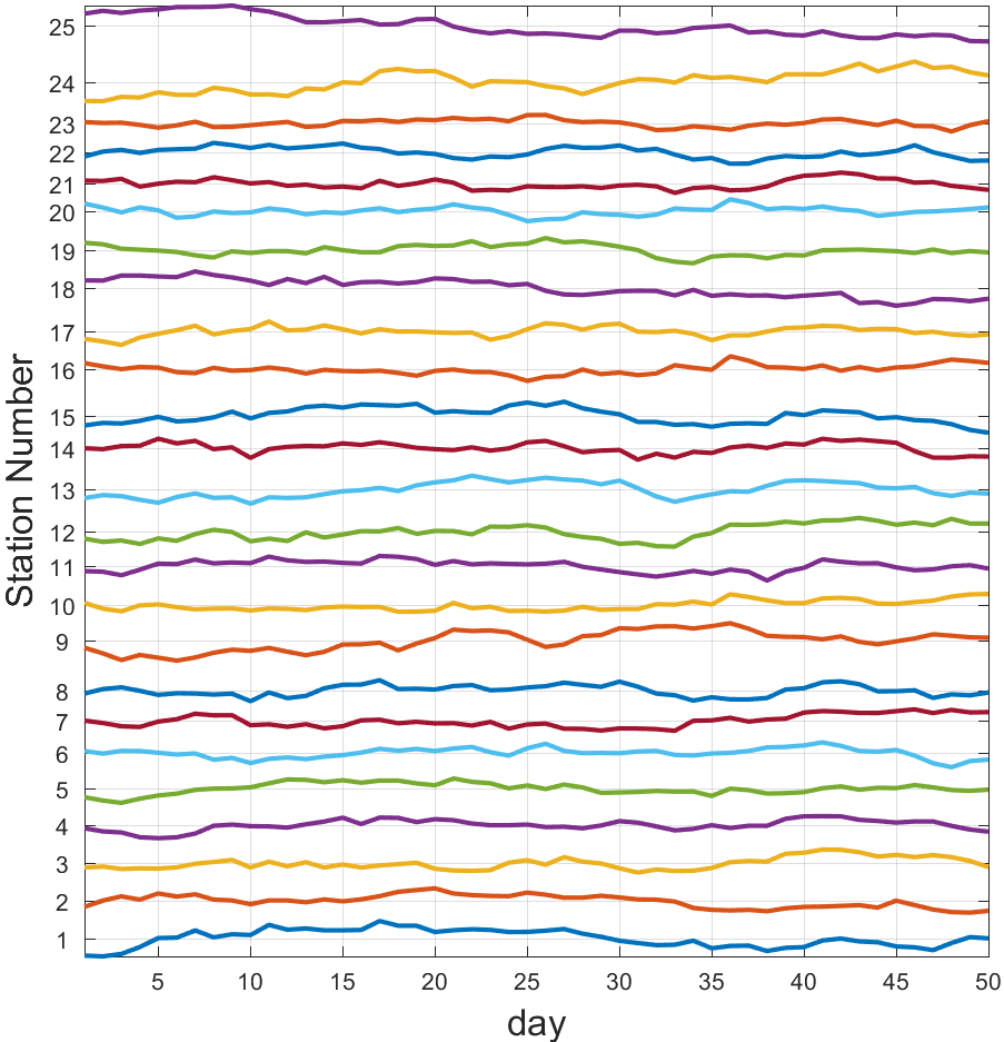
(a) Time series

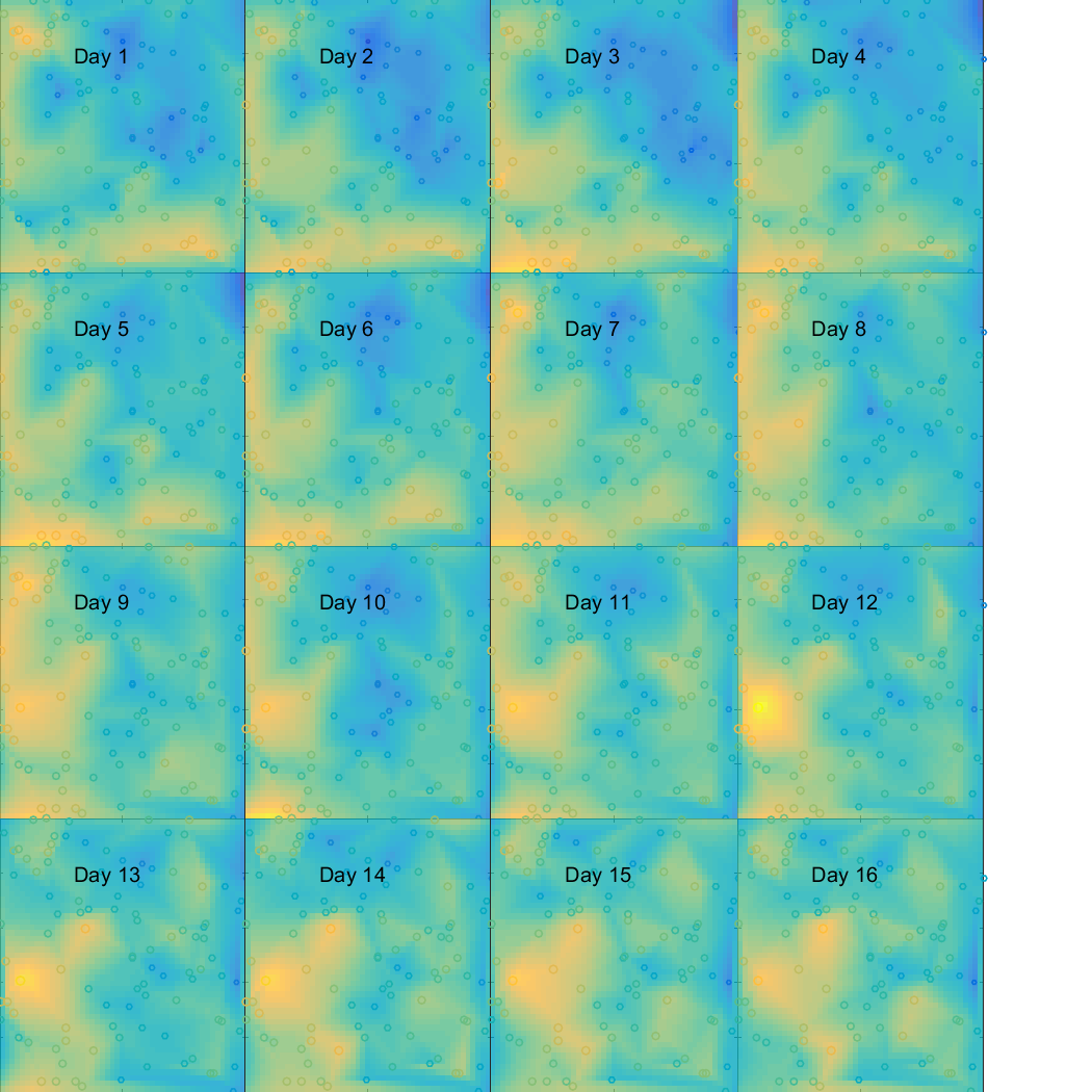
(b) Time slices

Figure 2: (a): Time series of synthetic data at 25 locations. (b): Spatial linear-interpolation maps for the first 16 time slices. The open circles represent the sampling locations. Each time slice corresponds to one simulated day.

5.1.1 SLI parameter estimation using MLE

We assume that the trend model is simply a constant term, i.e., $b_{1}$. The optimal model parameters are estimated by minimizing the NLL given by (24). The orders of the spatial and temporal neighbors are set to $K_{s}=K_{t}=3$. The initial guesses for the SLI parameters and the parameter bounds are given in Table 1. The value of the cost function (NLL) for the optimal SLI parameters is $\approx-1.4578\times 10^{4}$. The values of the optimal SLI parameters are listed in Table 1.

The sparsity pattern of the precision matrix evaluated with the optimal SLI parameters is shown in Fig. 3. The non-zero matrix entries are shown as blue dots. The four diagonal bands (two above and two below the main diagonal) comprise nearest and next-nearest temporal neighbors. The sparsity of the precision matrix is evident in the plot; the sparsity index is $\approx 0.13\%$ corresponding to 32 224 non-zero elements.

\begin{overpic}[scale={0.75}]{Figure3.pdf} \put(15.0,15.0){\includegraphics[scale={0.32}]{Figure3-det}} \end{overpic}

Figure 3: Sparsity pattern of the SLI precision matrix for the synthetic ST data; $nz=32\,224$ is the number of non-zero elements in the matrix, leading to a sparsity index of $\approx 0.13\%$. The inset figure shows a detail of the precision matrix.

	${m_{{\rm x}}}$	$\lambda$	$c_{1}$	$\mu_{t}$	$\mu_{s}$
Initial values	9.7424	430	$2.8484\times 10^{6}$	0.5	1
Lower bounds	9.5798	$10^{-3}$	1	1.4	0.4
Upper bounds	9.9050	$10^{7}$	$10^{7}$	10	10
Based on MLE	9.7424	0.001	4951.7	1.4	0.40

Table 1: SLI parameters for the synthetic ST data based on MLE. The initial guesses for the optimization are determined by running leave-one-out cross validation using root mean square error as the cost function. The lower and upper bounds on the mean are based on $\overline{x}\mp{5s_{x}}/{\sqrt{N}}$, where $\overline{x}$ is the sample mean, $s_{x}$ is the sample standard deviation, and $N=5000$ is the total number of points.

5.1.2 SLI model performance

To test the performance of the estimated SLI model we use one-slice-out cross validation: we remove and subsequently predict all the values for one time slice using the sample values at the $N_{t}-1$ remaining time slices. We repeat this experiment by removing sequentially all the time slices, one at a time. The scatter plot of the predictions (for all $N$ points) versus the sample values is shown in Fig. 4(a) and exhibits overall good agreement between the two sets. The histogram plots of the predicted versus the sample values, shown in Fig. 4(b), demonstrate that the SLI predictions tend to cluster around the center of the distribution more than the sample values.

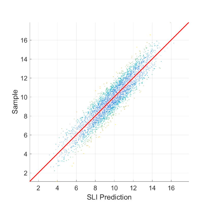
(a) Scatter plot

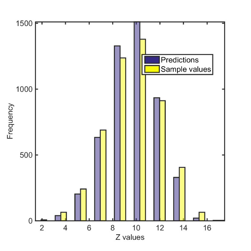
(b) Histogram

Figure 4: (a): Scatter plot of the predictions versus the sample values for the synthetic space-time data. (b): Histograms of the sample (yellow) and SLI-predicted (grey) values.

Cross validation measures are presented in Table 2: ME stands for the mean error (bias), MAE is the mean absolute error, MARE is the mean absolute relative error ($\approx 7.1\%$), RMSE is the root mean square error, RMSRE is the root mean square relative error ($\approx 10.49\%$), $R$ is the linear correlation coefficient ($\approx 0.94$) and $R_{S}$ the Spearman correlation coefficient (also $\approx 0.93$). The validation measures indicate overall good performance of the SLI model with small bias $\approx-0.007$ and very good correlation $\approx 0.94$. The RMSE is $\approx 0.80$.

In Table 2 we also compare the SLI cross validation measures with those obtained by means of ST Ordinary Kriging (OK) [26, 27]. The latter is implemented using the function krigeST from the R package gstat. The covariance parameters are estimated by means of the method of moments (MoM), e.g. [2]. We report OK cross validation results with three different parameter sets: The first set (OK-Ex) comprises the parameters of the theoretical covariance function. The second set (OK-Est-1) is based on the optimal covariance model which is fitted to the MoM estimator using unconstrained optimization. Finally, the third set (OK-Est-2) is obtained by means of the same fitting procedure by means of constrained optimization which forces the model parameters to lie within specific intervals (see caption of Table 2). The SLI prediction performs better than OK-Est-1, but it is inferior to OK-Ex and OK-Est-2, while OK-Est-2 has the best performance. These results are not surprising, given that OK employs the exponential covariance model that was used to generate the data. Nonetheless, the SLI performance is competitive with that of OK.

Method	ME	MAE	MARE	RMSE	RMSRE	$R$	$R_{S}$
SLI	$-$0.0070	0.6361	0.0717	0.7980	0.1049	0.9383	0.9347
OK-Ex	0.0003	0.6057	0.0684	0.7591	0.1015	0.9444	0.9401
OK-Est-1	0.0031	0.7807	0.0887	0.9819	0.1326	0.9069	0.8996
OK-Est-2	$-$0.0011	0.5920	0.0661	0.7398	0.0918	0.9468	0.9425

Table 2: One-slice-out cross validation (CV) interpolation performance for the Gaussian data with separable exponential covariance. The CV measures are calculated by comparing the true values of each time slice (from 1 to 50) and the predicted values. The predictions are based on $N_{t}-1$ time slices that exclude the predicted slice. First row: Predictions based on SLI. Second row (OK-Ex): Predictions based on Ordinary Kriging with theoretical covariance parameters. Third row (OK-Est-1): Predictions based on Ordinary Kriging with estimated covariance parameters (unconstrained estimates). Fourth row (OK-Est-2): Predictions based on Ordinary Kriging with estimated covariance parameters using constraints: $\xi_{s}\in[10,30]$, $\xi_{t}\in[5,15]$, nugget variance $\in[0,0.1]$, $\sigma^{2}\in[2.5,7.5]$.

5.2 Hourly temperature reanalysis data

We use ERA5 reanalysis temperature data (degrees Celsius) downloaded from the Copernicus Climate Change Service [28]. The dataset includes 39 000 points that correspond to hourly values for five consecutive days (January 1-5, 2017) at the nodes of a $13\times 25$ spatial grid around the island of Crete (Greece) as shown in Fig 5(a). The average spatial resolution is $\approx 0.28$ degrees (grid cell size $\approx 31$km). The data are displayed as time series in Fig. 5(b).

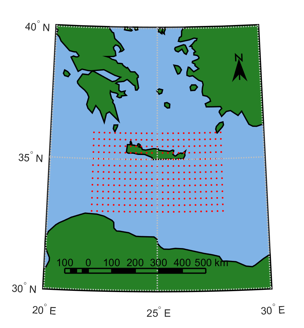
(a) Map showing the grid sites (red markers) of the ERA5 reanalysis data around the island of Crete that are used in the temperature analysis in Section 5.2.

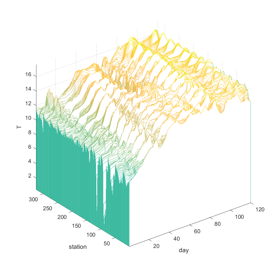
(b) Temperature

Figure 5: (a): Spatial grid for the ERA5 temperature data (degrees Celsius) around the island of Crete (Greece). (b): Time series of temperature (in degrees Celsius) at the ERA5 grid sites shown in (a).

The temperature data exhibit a clear increasing trend in time during the studied period. This is evidenced in the plot of the spatially averaged temperature as a function of time in Fig. 6, and the temperature fit with the linear regression model ${m_{{\rm x}}}(t)=b_{1}+b_{2}t+b_{3}t^{2}$ (where $t$ is measured in days). Thus, the parameter vector (13) with $K_{s}=K_{t}=3$ is given by ${\bm{\theta}}=\left(b_{1},b_{2},b_{3},\lambda,c_{1},\mu_{s},\mu_{t},3,3\right)^{\top}$.

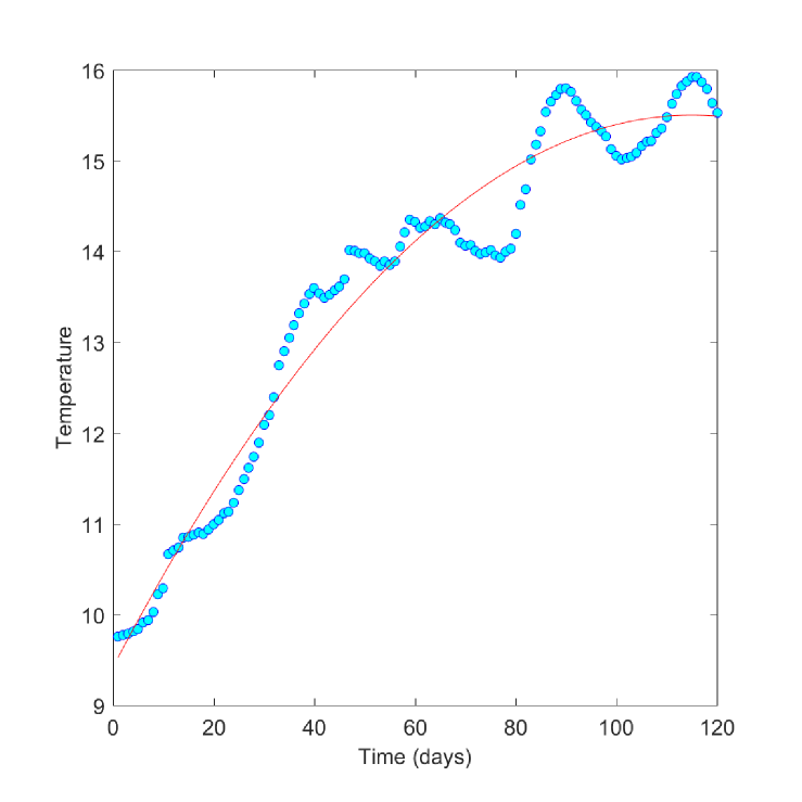
Figure 6: Plot of the spatially averaged temperatures (in degrees Celsius) as a function of time and least-squares fit to a second-degree polynomial function.

The SLI parameter estimation and the performance assessment are carried out as in the synthetic data case study (Section 5.1). The parameter estimates are shown in Table 3. The precision matrix has a sparsity index $\approx 0.006\%$, corresponding to $931\,070$ non-zero entries out of $1.521\times 10^{9}$ entries.

The scatter plot of the predictions (for all $N$ points) is shown in Fig. 7(a) and exhibits good agreement between the predictions and the data. The histogram plots of the predicted versus the sample values (Fig. 7(b)) also show that SLI predictions have lower dispersion than the sample values, as was the case for the synthetic data. The cross validation measures (obtained by sequentially removing each of the 120 hourly time slices) are shown in Table 4 and confirm the interpolation performance for the SLI model.

	$b_{1}$	$b_{2}$	$b_{3}$	$c_{1}$	$\mu_{t}$	$\mu_{s}$	$\lambda$
Initial	9.4203	0.1058	$-4.6\times 10^{-4}$	300	3	2.5	10
L.B.	9.2042	0.0975	$-5.26\times 10^{-4}$	1	1	1	1
U.B.	9.6363	0.1140	$-3.94\times 10^{-4}$	1000	1000	10	10
MLE	9.5587	0.1019	$-0.0004$	111.4797	1	1	1 $\times 10^{-4}$

Table 3: SLI model parameters for the ERA5 temperature data based on MLE. The initial values for $b_{1},b_{2},b_{3}$ are obtained from the coefficients of the regression model for the trend. The lower (L.B.) and upper (U.B.) bounds of the coefficients are the respective limits of the regression-based 95% confidence intervals.

ME (∘C)	MAE (∘C)	MARE	RMSE (∘C)	RMSRE	$R$	$R_{S}$
$-0.0008$	0.1022	0.0085	0.1737	0.0216	0.9971	0.9969

Table 4: One-slice-out cross validation (CV) test of the SLI interpolation performance for the ERA5 temperature data. The CV measures are calculated by comparing the true temperature values of each hourly time slice (from 1 to 120) and the SLI predictions that are based on the SLI model with the MLE parameters reported in Table 3. The predictions are based on $N_{t}-1$ time slices excluding the predicted slice.

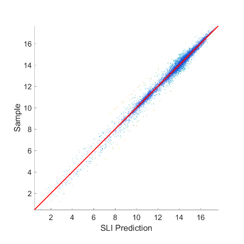
(a) Scatter plot

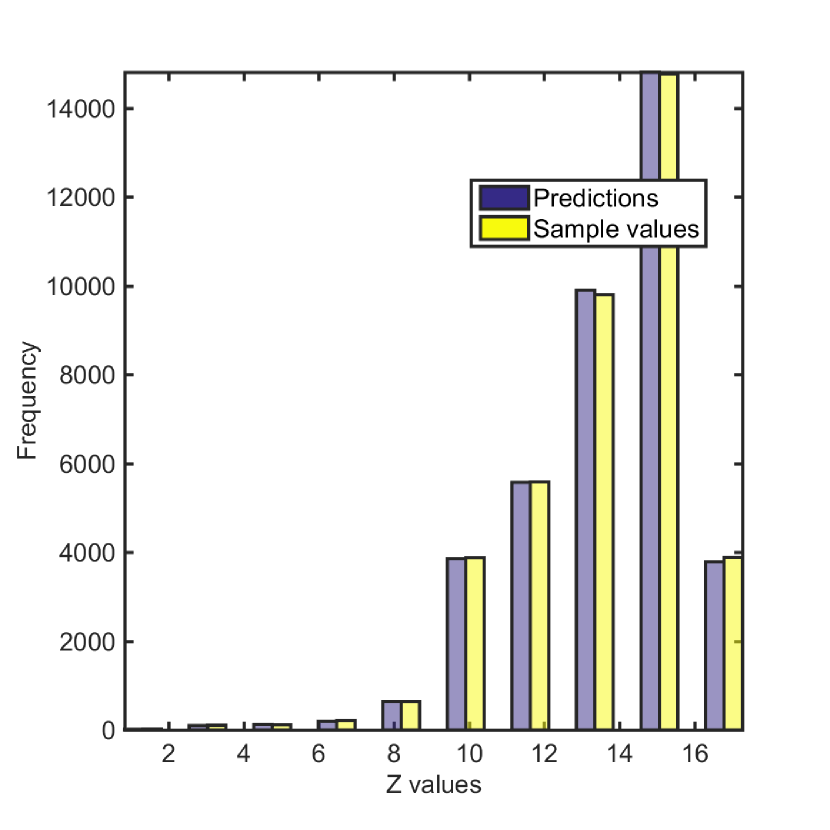
(b) Histogram

Figure 7: (a): Scatter plot of the SLI predictions versus the sample values for the ERA5 temperature data. (b): Histograms of the sample (yellow) and SLI-predicted (grey) values.

5.3 Hourly ozone concentration data

This dataset includes ozone (O₃) hourly concentration data (measured in $\mu$g/m³) for five consecutive days (July 1-5, 2014), downloaded from the French GEOD’AIR database (web site: www.prevair.org). The data are collected at 335 scattered stations distributed around France. The time series at 107 stations that reported data at all times are shown in Fig. 8(a). Linear interpolation maps for the first 16 time slices are shown in Fig. 8(b).

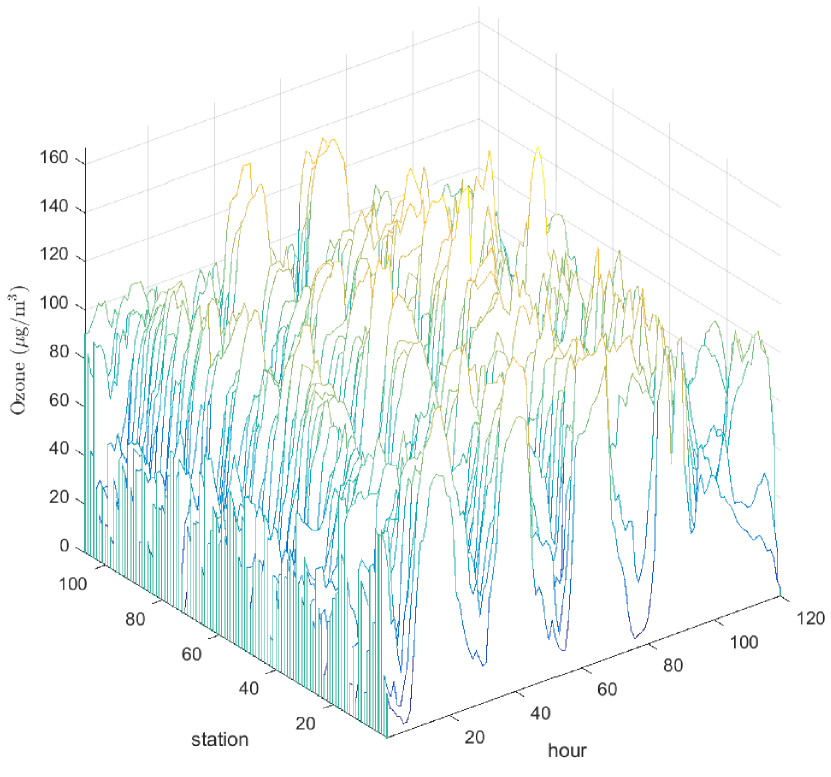
(a) Time series

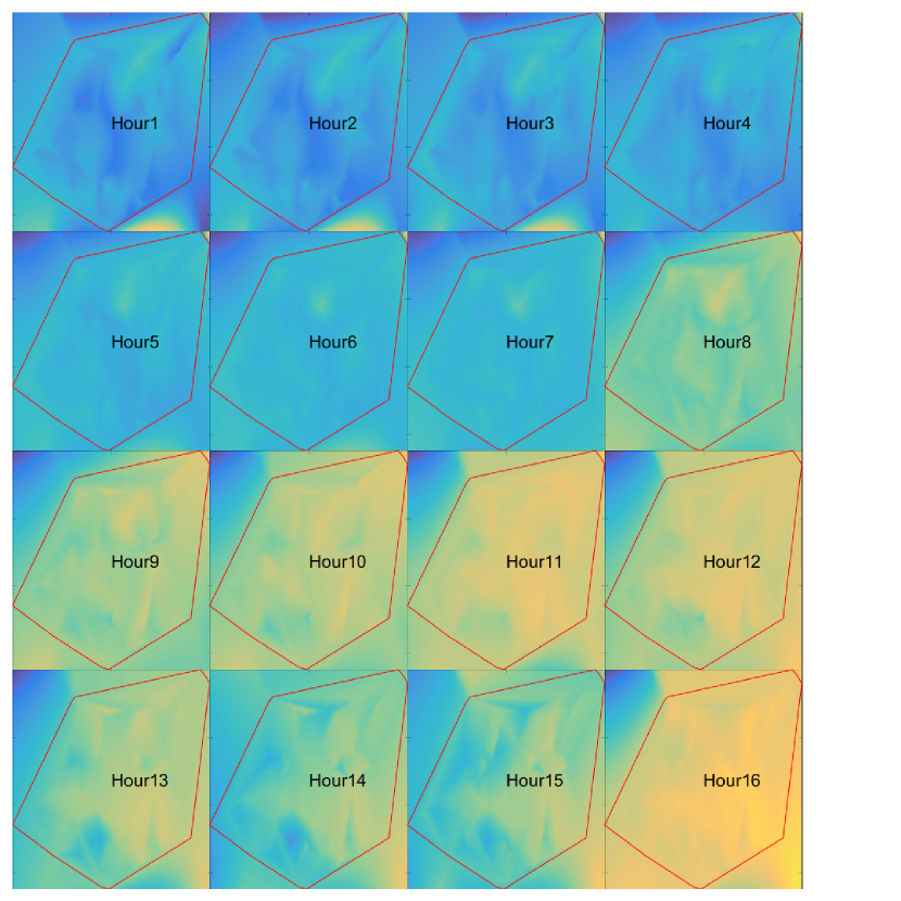
(b) Time slices

Figure 8: (a): Time series of ozone O₃ hourly data ($\mu$g/m³) at 107 stations in France and spatial linear-interpolation maps for the first 16 hourly time slices. (b): Linear interpolation maps of ozone concentration for different time slices (hours of the day). The red polygon marks the convex hull of the station network.

A visual inspection of the spatially averaged ozone time series indicates the existence of a temporal trend which is modeled by means of the following function which exhibits daily (24-hr) periodicity

$${m_{{\rm x}}}(t)=b_{1}+\left(b_{2}+b_{3}t+b_{4}t^{2}\right)\cos\left(\frac{2\pi t}{24}\right)+\left(b_{5}+b_{6}t+b_{7}t^{2}\right)\sin\left(\frac{2\pi t}{24}\right).$$ (25)

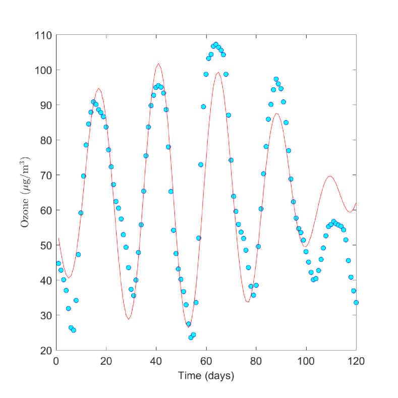
Figure 9: Plot of the spatially averaged ozone concentration ($\mu$g/m³) over the study domain as a function of time (circles) and least-squares fit to the temporal trend function given by (25).

The SLI parameter estimation is conducted using MLE. The parameter estimates are shown in Table 5. MARE and RMSRE are infinite because the dataset includes zero values. The precision matrix has a sparsity index $\approx 0.07\%$, i.e., it includes $1.154\times 10^{5}$ non-zero entries out of $1.649\times 10^{8}$ entries.

	$b_{1}$	$b_{2}$	$b_{3}$	$b_{4}$	$b_{5}$	$b_{6}$	$b_{7}$	$c_{1}$	$\mu_{t}$	$\mu_{s}$	$\lambda$
Initial	64.05	$-7.19$	$-0.14$	$1.5\times 10^{-3}$	$-18.59$	$-0.77$	$8\times 10^{-3}$	1	3	2.5	1
L.B.	62.13	$-15.50$	$-0.45$	$-10^{-3}$	$-26.84$	$-1.08$	$5.6\times 10^{-3}$	$10^{-3}$	0.5	0.5	$10^{-3}$
U.B.	65.97	$1.12$	$0.17$	$4\times 10^{-3}$	$-10.34$	$-0.45$	$0.011$	$10^{7}$	10	10	$10^{7}$
MLE	63.64	$-7.67$	$-0.14$	$1.6\times 10^{-3}$	$-19.57$	$-0.57$	$5.6\times 10^{-3}$	77.63	1.17	0.5	$10^{-3}$

Table 5: SLI model parameters for the French ozone concentration data based on MLE. The initial values for the trend coefficients $\{b_{i}\}_{i=1}^{7}$ are obtained from the coefficients of the regression model for the trend (25). The lower (L.B.) and upper (U.B.) bounds of the coefficients are the limits of the respective regression-based 95% confidence intervals. The value of the cost functional (NLL) at the optimum is equal to $-5.471\times 10^{-3}$.

The scatter plot of the predictions (for all $N$ points) versus the sample values is shown in Fig. 10(a) and exhibits overall good agreement between the data and the predictions. The histogram plots of the predicted versus the sample values, shown in Fig. 10(b) also show that SLI predictions have lower dispersion than the sample values as in the case of synthetic data. The cross validation performance measures (obtained by sequentially removing each of the 120 hourly time slices) are shown in Table 6, and they demonstrate very good interpolation performance for the SLI model. Note that $\mu_{s}=0.5$, which implies that the spatial bandwidth is small. On the other hand, $\mu_{t}\approx 1.17$ and $K_{t}=3$ imply that the temporal bandwidth is $\mu_{t}(K_{t}-1)\delta t\approx 2.34$ hr ($\delta t=1$ hour). This result implies that the SLI predictions are at most locations based on the four temporal nearest neighbors (two forward and two backward). For the first and last time slices the bandwidth is $K_{t}\,\mu_{t}\delta t=3.50$ hr.

ME ($\mu$g/m3)	MAE ($\mu$g/m3)	MARE	RMSE ($\mu$g/m3)	RMSRE	$R$	$R_{S}$
0.00853	6.0941	Inf	8.503	Inf	0.96	0.96

Table 6: Cross validation (CV) interpolation performance measures for the ozone concentration values. The CV measures compare the true ozone concentration values ($\mu g/m^{3}$) of each hourly time slice (from 1 to 120) with the SLI predictions. The latter are based on $N_{t}-1$ time slices that exclude the predicted slice.

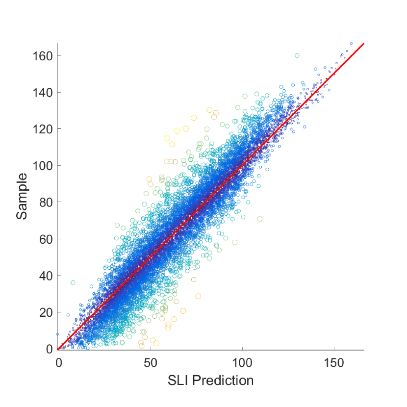
(a) Scatter plot

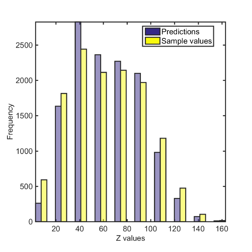
(b) Histogram

Figure 10: (a): Scatter plot of the SLI predictions versus the sample values for the French hourly ozone data. (b): Histograms of the sample (yellow) and SLI-predicted (grey) values.

6 Discussion and Conclusions

We present a theoretical framework for constructing ST models based on exponential Boltzmann-Gibbs joint probability density functions. The ST-SLI model presented herein exploits an energy function with local interactions which imposes sparse structure on the precision matrix. The local interactions are implemented by means of compactly supported kernel functions that compensate for the lack of a structured lattice. However, the model is also applicable to regular lattice data. In this case the SLI model is equivalent to a Gauss Markov random field with a specific precision matrix structure. To our knowledge, this structure that involves kernel-matrix weights has not been used before in models of real-valued ST data. The ST-SLI model extends the purely spatial SLI model [13] to the space-time domain. The SLI approach shares the reliance on kernel functions with kernel-based reconstruction of graph signals [29]. In the case of environmental ST data, the graph topology is not given a priori, but it is determined from the data by optimizing the negative likelihood of the model.

The SLI model presented features a Gaussian energy functional with a sparse precision matrix. Explicit expressions are given for ST prediction and the conditional variance at the prediction sites. The sparse precision matrix representation allows computationally efficient implementation of parameter estimation and prediction procedures. The computational efficiency stems from the fact that in SLI it is not necessary to store and invert large and dense covariance matrices.

The optimization of the cost function (the negative logarithmic likelihood) was based on the interior-point algorithm which terminates at local minima. The landscape of the cost function should be further investigated in order to understand the patterns of local minima. It is also possible to run a global optimization algorithm to search for the global optimum of the cost function. On the other hand, experience with the purely spatial SLI model [13] shows that local minima of the cost function provide parameter estimates that are sufficient for interpolation purposes.

In terms of prediction performance, we have shown (see Table 2) that for synthetic data the SLI cross validation statistics are slightly inferior but competitive with those obtained by means of Ordinary kriging. This behavior is observed in spite of the fact that Ordinary kriging has the advantage of employing the functional form (exponential) of the covariance model used to generate the data. In our experience with performance comparisons based on spatial data, the ranking of different methods with regard to prediction performance may change depending on the specific data set. In our opinion, the results shown herein establish that SLI is a competitive method for space-time data interpolation. Further studies can elaborate on the performance of SLI relative to other methods.

The formulation presented herein can be extended to multivariate random fields by suitable selection of the energy function. In addition, it is possible to include anisotropic and more general (e.g., geodesic) spatial distance metrics in the kernel functions, periodic patterns (in space and in time) by adding shifted averaged squared increments, and spatial dependence of the coefficients $\lambda$ and $c_{1}$. Such extensions will enhance the flexibility of the SLI model at the cost of some loss in computational efficiency.

References

- [1] National Research Council et al. Frontiers in Massive Data Analysis. National Academies Press, Washington, DC, 2013.
- [2] J. P. Chilès and P. Delfiner. Geostatistics: Modeling Spatial Uncertainty. Wiley, New York, 2nd edition, 2012.
- [3] C. E. Rasmussen and C. K. I. Williams. Gaussian Processes for Machine Learning. MIT Press, Massachusetts Institute of Technology, 2006.
- [4] G. Christakos. Random Field Models in Earth Sciences. Academic Press, San Diego, 1992.
- [5] N. Cressie and C. L. Wikle. Statistics for Spatio-temporal Data. John Wiley and Sons, New York, 2011.
- [6] S. De Iaco, D. E. Myers, and D Posa. Nonseparable space-time covariance models: some parametric families. Mathematical Geology, 34(1):23–42, 2002.
- [7] A. Kolovos, G. Christakos, D.T. Hristopulos, and M. L. Serre. Methods for generating non-separable spatiotemporal covariance models with potential environmental applications. Advances in Water Resources, 27(8):815–830, 2004.
- [8] E. A. Varouchakis and D. T. Hristopulos. Comparison of spatiotemporal variogram functions based on a sparse dataset of groundwater level variations. Spatial Statistics, 34:100245, 2019.
- [9] T. Gneiting, M. G. Genton, and P. Guttorp. Geostatistical space-time models, stationarity, separability, and full symmetry. In B. Finkelstádt, L. Held, and V. Isham, editors, Statistical Methods for Spatio-Temporal Systems, volume 107, pages 151–175. Chapman & Hall, 2006.
- [10] Y. Sun, B. Li, and M. G. Genton. Geostatistics for large datasets. In E. Porcu, J.–M. Montero, and M. Schlather, editors, Advances and Challenges in Space-time Modelling of Natural Events, Lecture Notes in Statistics, pages 55–77. Springer Berlin Heidelberg, 2012.
- [11] G. Mussardo. Statistical Field Theory. Oxford University Press, Oxford, 2010.
- [12] H. Rue and L. Held. Gaussian Markov Random Fields: Theory and Applications. Chapman and Hall/CRC, Boca Raton, FL, 2005.
- [13] D. T. Hristopulos. Stochastic local interaction (SLI) model: Bridging machine learning and geostatistics. Computers & Geosciences, 85(Part B):26–37, 2015.
- [14] D. T. Hristopulos and I. C. Tsantili. Space–time covariance functions based on linear response theory and the turning bands method. Spatial Statistics, 22, Part 2:321–337, 2017.
- [15] E. Koutroulis and D. Kolokotsa. Design optimization of desalination systems power-supplied by PV and W/G energy sources. Desalination, 258(1-3):171–181, 2010.
- [16] A. Bárdossy and G. Pegram. Infilling missing precipitation records–a comparison of a new copula-based method with other techniques. Journal of hydrology, 519, Part A:1162–1170, 2014.
- [17] M. Kardar. Statistical Physics of Fields. Cambridge University Press, 2007.
- [18] E. Ising. Beitrag zur theorie des ferromagnetismus. Zeitschrift für Physik, 31(1):253–258, 1925.
- [19] J. Besag. Spatial interaction and the statistical analysis of lattice systems. Journal of the Royal Statistical Society. Series B (Methodological), 36(2):192–236, 1974.
- [20] E. A. Nadaraya. On estimating regression. Theory of Probability and its Applications, 9(1):141–142, 1964.
- [21] G. S. Watson. Smooth regression analysis. Sankhya Ser. A, 26(1):359–372, 1964.
- [22] G. Christakos, D. T. Hristopulos, and P. Bogaert. On the physical geometry concept at the basis of space/time geostatistical hydrology. Advances in Water Resources, 23(8):799–810, 2000.
- [23] G. Christakos. Spatiotemporal Random Fields: Theory and Applications. Elsevier, Amsterdam, Netherlands, 2017.
- [24] M. Schlather, A. Malinowski, M. Oesting, D. Boecker, K. Strokorb, S. Engelke, J. Martini, F. Ballani, O. Moreva, J. Auel, P. J. Menck, S. Gross, U. Ober, C. Berreth, K. Burmeister, J. Manitz, P. Ribeiro, R. Singleton, B. Pfaff, and R Core Team. RandomFields: Simulation and Analysis of Random Fields, 2017. R package version 3.1.50.
- [25] M. Schlather, A. Malinowski, P. J. Menck, M. Oesting, and K. Strokorb. Analysis, simulation and prediction of multivariate random fields with package RandomFields. Journal of Statistical Software, 63(8):1–25, 2015.
- [26] E. Pebesma and G. Heuvelink. Spatio-temporal interpolation using gstat. RFID Journal, 8(1):204–218, 2016.
- [27] C. K. Wikle, A. Zammit-Mangion, and N. Cressie. Spatio-temporal Statistics with R. CRC Press, Boca Raton, FL, 2019.
- [28] Copernicus Climate Change Service C3S. ERA5: Fifth generation of ECMWF atmospheric reanalyses of the global climate, 2018. Data retrieved from: https://cds.climate.copernicus.eu/cdsapp#!/home.
- [29] D. Romero, M. Ma, and G. B. Giannakis. Kernel-based reconstruction of graph signals. IEEE Transactions on Signal Processing, 65(3):764–778, 2017.