An LMI Condition for the Robustness of Constant-Delay Linear Predictor Feedback with Respect to Uncertain Time-Varying Input Delays

Abstract

This paper discusses the robustness of the constant-delay predictor feedback in the case of an uncertain time-varying input delay. Specifically, we study the stability of the closed-loop system when the predictor feedback is designed based on the knowledge of the nominal value of the time-varying delay. By resorting to an adequate Lyapunov-Krasovskii functional, we derive an LMI-based sufficient condition ensuring the exponential stability of the closed-loop system for small enough variations of the time-varying delay around its nominal value. These results are extended to the feedback stabilization of a class of diagonal infinite-dimensional boundary control systems in the presence of a time-varying delay in the boundary control input.

, , ,

1 Introduction

Originally motivated by the work of Artstein [1], linear predictor feedback is an efficient tool for the feedback stabilization of Linear Time-Invariant (LTI) systems with constant input delay. In particular, predictor feedback can be used for controlling plants that are open-loop unstable and in the presence of large input delays. Many extensions have been reported (see, e.g., [14] and the references therein). These include the case of time-varying delay linear predictor feedback [16]; robustness with respect to disturbance signals [5]; truncated predictor [23]; predictor observers in the case of sensor delays [14]; predictors for nonlinear systems [3, 15]; dependence of the delay on the state [2]; networked control [22]; and the boundary control of partial differential equations [17, 20].

Most of the predictor feedback strategies reported in the literature assume a perfect knowledge in real-time of the input delay. However, such an assumption might be difficult to fulfill in practice. Consequently, there has been an increased interest in the last decade for the study of the robustness of the predictor feedback with respect to delay mismatches. An example of such a problem was investigated in [12] where the exponential stability of the closed-loop system was assessed for unknown constant delays with small enough deviations from the nominal value. The study of the impact of an unknown time-varying delay, but with known nominal value which is used to design the predictor feedback, on the system closed-loop stability was reported in [3]. In particular, it was shown that the exponential stability of the closed-loop system is guaranteed for sufficiently small variations of the delay in both amplitude and rate of variation. Such an approach was further investigated in [10] where a small gain condition on the only amplitude of variation of the delay around its nominal value was derived for ensuring the exponential stability of the closed-loop system. However, as underlined in [19], such a small gain condition might be conservative as it involves norms of matrices which generally grow quickly with their dimensions. In order to reduce such a conservatism, it was proposed in [19] to resort to a Lyapunov-Krasovskii functional approach in the case of constant uncertain delays. By doing so, an LMI-based sufficient condition, was derived, for ensuring the asymptotic stability of the closed-loop system with constant uncertain delays.

The first contribution of this paper deals with the study of the robustness of the constant-delay predictor feedback that has been designed based on the nominal value of an uncertain and time-varying input delay. By taking advantage of classical Lyapunov-Krasovskii functionals [9], we derive an LMI-based sufficient condition on the amplitude of variation of the input delay around its nominal value that ensures the exponential stability of the closed-loop system. Such an approch was investigated first in [22] in the context of networked control. However, the LMI condition derived in this paper differs from the one proposed in [22]. Three examples are developed showing that, for these case studies, the LMI condition proposed in this paper provides less conservative results than the small gain condition reported in [10] and the LMI condition extracted from [22].

The second contribution of this paper deals with the extension of the above result to the feedback stabilization of a class of diagonal infinite-dimensional boundary control systems [7] in the presence of a time-varying delay in the boundary control input. The control strategy consists in 1) the use of a predictor feedback to stabilize a finite-dimensional subsystem capturing the unstable modes of the infinite-dimensional system; 2) ensuring that the control law designed on a finite-dimensional truncated models successfully stabilizes the full infinite-dimensional system. Such a control strategy, inspired by [21] in the case of a delay-free feedback control, was first reported in [20] for the exponential stabilization of a reaction-diffusion equation with a constant delay in the boundary control. Note that a different approach for tackling the same feedback stabilization problem was reported in [13] via the use of a backstepping boundary controller. Ideas from [20] were extended to the exponential stabilization of a class of diagonal infinite-dimensional boundary control systems with constant delay in the boundary control in [17]. In this present paper, we go beyond [13, 17, 20] and assess the robustness of the control strategy reported in [17] in the case of an uncertain and time-varying input delay. Specifically, we show that for time-varying delays presenting 1) a sufficiently small amplitude of variation around its nominal value (with sufficient condition provided by the LMI condition discussed above); 2) a rate of variation that is bounded by an arbitrarily large constant; the infinite-dimensional closed-loop system is exponentially stable.

The remainder of this paper is organized as follows. The robustness of the predictor feedback with respect to uncertain and time-varying delays is investigated in Section 2. The extension of this result to the feedback stabilization of a class of diagonal infinite-dimensional boundary control systems is presented in Section 3. The obtained results are applied in Section 4. Finally, concluding remarks are provided in Section 5.

Notation. The sets of non-negative integers, positive integers, real, non-negative real, positive real, and complex numbers are denoted by $\mathbb{N}$, $\mathbb{N}^{*}$, $\mathbb{R}$, $\mathbb{R}_{+}$, $\mathbb{R}_{+}^{*}$, and $\mathbb{C}$, respectively. The real and imaginary parts of a complex number $z$ are denoted by $\operatorname{Re}z$ and $\operatorname{Im}z$, respectively. The field $\mathbb{K}$ denotes either $\mathbb{R}$ or $\mathbb{C}$. The set of $n$-dimensional vectors over $\mathbb{K}$ is denoted by $\mathbb{K}^{n}$ and is endowed with the Euclidean norm $\|x\|=\sqrt{x^{*}x}$. The set of $n\times m$ matrices over $\mathbb{K}$ is denoted by $\mathbb{K}^{n\times m}$ and is endowed with the induced norm denoted by $\|\cdot\|$. For any symmetric matrix $P\in\mathbb{R}^{n\times n}$, $P\succ 0$ (resp. $P\succeq 0$) means that $P$ is positive definite (resp. positive semi-definite). The set of symmetric positive definite matrices of order $n$ is denoted by $\mathbb{S}_{n}^{+*}$. For any symmetric matrix $P\in\mathbb{R}^{n\times n}$, $\lambda_{m}(P)$ and $\lambda_{M}(P)$ denote the smallest and largest eigenvalues of $P$, respectively. For $M=(m_{i,j})\in\mathbb{C}^{n\times m}$, we introduce

$$\mathcal{R}(M)\triangleq\begin{bmatrix}\operatorname{Re}M&-\operatorname{Im}M\\ \operatorname{Im}M&\operatorname{Re}M\end{bmatrix}\in\mathbb{R}^{2n\times 2m}$$

where $\operatorname{Re}M\triangleq(\operatorname{Re}m_{i,j})\in\mathbb{R}^{n\times m}$ and $\operatorname{Im}M\triangleq(\operatorname{Im}m_{i,j})\in\mathbb{R}^{n\times m}$. For any $t_{0}>0$, we say that $\varphi\in\mathcal{C}^{0}(\mathbb{R};\mathbb{R})$ is a transition signal over $[0,t_{0}]$ if $0\leq\varphi\leq 1$, $\left.\varphi\right|_{(-\infty,0]}=0$, and $\left.\varphi\right|_{[t_{0},+\infty)}=1$. In Section 3, the notations and terminologies for infinite-dimensional systems are retrieved from [7].

2 Delay-robustness of predictor feedback for LTI systems

2.1 Problem setting and existing result

The first part of this paper deals with the feedback stabilization of the following LTI system with delay control:

$$\dot{x}(t)=Ax(t)+Bu(t-D(t)),\quad t\geq 0,$$ (1)

with $A\in\mathbb{R}^{n\times n}$ and $B\in\mathbb{R}^{n\times m}$ such that the pair $(A,B)$ is stabilizable. Vectors $x(t)\in\mathbb{R}^{n}$ and $u(t)\in\mathbb{R}^{m}$ denote the state and the control input, respectively. The command input is subject to an uncertain time-varying delay $D\in\mathcal{C}^{0}(\mathbb{R}_{+};\mathbb{R}_{+})$. We assume that there exist $D_{0}>0$ and $0<\delta<D_{0}$ such that $|D(t)-D_{0}|\leq\delta$ for all $t\geq 0$. In this context, the following constant-delay linear predictive feedback, which is based on the knowledge of the constant nominal value $D_{0}$, has been proposed in [3]:

$$u(t)=K\left\{e^{D_{0}A}x(t)+\int_{t-D_{0}}^{t}e^{(t-s)A}Bu(s)\mathop{}\!\mathrm{d}s\right\}$$ (2)

for $t\geq 0$, where $K\in\mathbb{R}^{n\times m}$ is a feedback gain such that $A_{\mathrm{cl}}\triangleq A+BK$ is Hurwitz. The validity of such a control strategy was assessed in [10] via a small gain argument.

Theorem 1 ([10]).

Let $D_{0}>0$ be given and let $A\in\mathbb{R}^{n\times n}$, $B\in\mathbb{R}^{n\times m}$, and $K\in\mathbb{R}^{m\times n}$ be such that $A_{\mathrm{cl}}=A+BK$ is Hurwitz. Let $\delta\in(0,D_{0})$ be such that

$$M\|e^{D_{0}A}BK\|\left\{e^{\|A_{\mathrm{cl}}\|\delta}-e^{-\mu\delta}\right\}<\mu,$$ (3)

where $M,\mu>0$ are constants satisfying $\|e^{A_{\mathrm{cl}}t}\|\leq Me^{-\mu t}$ for all $t\geq 0$. Then, there exists $N,\sigma>0$ such that for all $x_{0}\in\mathbb{R}^{n}$, $u_{0}\in\mathcal{C}^{0}([-D_{0}-\delta,0];\mathbb{R}^{m})$ with $u_{0}(0)=K\left\{e^{D_{0}A}x_{0}+\int_{-D_{0}}^{0}e^{-sA}Bu_{0}(s)\mathop{}\!\mathrm{d}s\right\}$, and $D\in\mathcal{C}^{0}(\mathbb{R}_{+};\mathbb{R}_{+})$ with $|D-D_{0}|\leq\delta$, the solution of (1-2) associated with the initial conditions $x(0)=x_{0}$ and $u(t)=u_{0}(t)$ for $-D_{0}-\delta\leq t\leq 0$ satisfies for all $t\geq 0$ the following estimate:

$$\|x(t)\|+\max\limits_{t-D_{0}-\delta\leq s\leq t}\|u(s)\|$$

$$\qquad\leq Ne^{-\sigma t}\left\{\|x_{0}\|+\max\limits_{-D_{0}-\delta\leq s\leq 0}\|u_{0}(s)\|\right\}.$$

As the left hand-side of (3) is equal to zero when $\delta=0$, a continuity argument shows that there always exists a $\delta>0$ such that (3) holds true. Therefore, Theorem 1 ensures the existence of a sufficiently small amplitude of perturbation $\delta>0$ of the delay $D(t)$ around its nominal value $D_{0}$ such that the constant-delay linear predictor feedback (2) ensures the exponential stability of the closed-loop system with uncertain time-varying input delays. However, due to the nature of the small gain-condition (3) that involves the norm of matrices (which generally grow quickly as a function of the matrices dimensions $n$ and $m$), the admissible values of $\delta$ might be conservative (see [19]). In particular, from the fact that $M\geq 1$ and $0<\mu\leq\mu_{M}(A_{\mathrm{cl}})\triangleq-\max\{\operatorname{Re}\lambda\,:\,\lambda\in\mathrm{sp}_{\mathbb{C}}(A_{\mathrm{cl}})\}$, any $\delta>0$ such that the small gain condition (3) holds true satisfies the following estimate:

$$\delta<\delta_{\mathrm{E}}\triangleq\dfrac{1}{\|A_{\mathrm{cl}}\|}\log\left(1+\dfrac{\mu_{M}(A_{\mathrm{cl}})}{\|e^{D_{0}A}BK\|}\right).$$ (4)

To reduce the conservatism, an LMI condition ensuring the exponential stability of the closed-loop system was derived in [22] in the context of networked control. The objective of this section it to propose the construction of an alternative LMI for such a problem. Numerical comparisons between the different methods (small gain and LMIs) will be carried out in Subsection 2.4 and Section 4.

2.2 Preliminary results

For $h>0$, we denote by $W$ the space of absolutely continuous functions $\psi:[-h,0]\rightarrow\mathbb{R}^{n}$ with square-integrable derivative endowed with the norm $\|\psi\|_{W}\triangleq\sqrt{\|\psi(0)\|^{2}+\int_{-h}^{0}\|\dot{\psi}(\theta)\|^{2}\mathop{}\!\mathrm{d}\theta}$ (see [11, Chap. 4, Sec. 1.3]).

Lemma 2.

Let $M,N\in\mathbb{R}^{n\times n}$, $D_{0}>0$, and $\delta\in(0,D_{0})$ be given. Assume that there exist $\kappa>0$, $P_{1},Q\in\mathbb{S}_{n}^{+*}$, and $P_{2},P_{3}\in\mathbb{R}^{n\times n}$ such that $\Theta(\delta,\kappa)\preceq 0$ with

$$\Theta(\delta,\kappa)=$$ (5)

$$\begin{bmatrix}2\kappa P_{1}+M^{\top}P_{2}+P_{2}^{\top}M&\;P_{1}-P_{2}^{\top}+M^{\top}P_{3}&\;\delta P_{2}^{\top}N\\ P_{1}-P_{2}+P_{3}^{\top}M&\;-P_{3}-P_{3}^{\top}+2\delta Q&\;\delta P_{3}^{\top}N\\ \delta N^{\top}P_{2}&\;\delta N^{\top}P_{3}&\;-\delta e^{-2\kappa D_{0}}Q\end{bmatrix}.$$

Then, there exists $C_{0}>0$ such that, for any $D\in\mathcal{C}^{0}(\mathbb{R}_{+};\mathbb{R}_{+})$ with $|D-D_{0}|\leq\delta$, the trajectory $x$ of:

$$\dot{x}(t) =Mx(t)+N\left\{x(t-D(t))-x(t-D_{0})\right\},\quad t\geq 0;$$

$$x(t) =x_{0}(t),\quad t\in[-D_{0}-\delta,0]$$

with initial condition $x_{0}\in W$ (for $h=D_{0}+\delta$) satisfies $\|x(t)\|\leq C_{0}e^{-\kappa t}\|x_{0}\|_{W}$ for all $t\geq 0$.

Proof. For all $t\geq 0$, one has

$$\dot{x}(t)=Mx(t)+N\int_{t-D_{0}}^{t-D(t)}\dot{x}(\tau)\mathop{}\!\mathrm{d}\tau.$$ (6)

Inspired by classical Lyapunov-Krasovskii functional depending on time derivative for systems with fast varying delays, see  [9, Sec. 3.2], we introduce $V(t)=V_{1}(t)+V_{2}(t)$ with $V_{1}(t)=x(t)^{\top}P_{1}x(t)$ and $V_{2}(t)=\int_{-D_{0}-\delta}^{-D_{0}+\delta}\int_{t+\theta}^{t}e^{2\kappa(s-t)}\dot{x}(s)^{\top}Q\dot{x}(s)\mathop{}\!\mathrm{d}s\mathop{}\!\mathrm{d}\theta$, where $P_{1},Q\in\mathbb{S}_{n}^{+*}$. Then we have, for all $t\geq 0$,

$$\dot{V}(t) =2x(t)^{\top}P_{1}\dot{x}(t)+2\delta\dot{x}(t)^{\top}Q\dot{x}(t)-2\kappa V_{2}(t)$$ (7)

$$\phantom{=}\,-\int_{-D_{0}-\delta}^{-D_{0}+\delta}e^{2\kappa\theta}\dot{x}(t+\theta)^{\top}Q\dot{x}(t+\theta)\mathop{}\!\mathrm{d}\theta.$$

The remaining of the proof is now an adaptation of [8, Proof of Thm 1]. Introducing $P=\begin{bmatrix}P_{1}&0\\ P_{2}&P_{3}\end{bmatrix}$, where $P_{2},P_{3}\in\mathbb{R}^{n\times n}$ are “slack variables” [9], we have

$$x(t)^{\top}P_{1}\dot{x}(t)$$

$$\overset{(\ref{eq: dynamics in function of dot_x})}{=}\begin{bmatrix}x(t)\\ \dot{x}(t)\end{bmatrix}^{\top}P^{\top}\begin{bmatrix}\dot{x}(t)\\ -\dot{x}(t)+Mx(t)+N\int_{t-D_{0}}^{t-D(t)}\dot{x}(\tau)\mathop{}\!\mathrm{d}\tau\end{bmatrix}$$

$$=\begin{bmatrix}x(t)\\ \dot{x}(t)\end{bmatrix}^{\top}P^{\top}\begin{bmatrix}0&I\\ M&-I\end{bmatrix}\begin{bmatrix}x(t)\\ \dot{x}(t)\end{bmatrix}$$ (8)

$$\phantom{=}\;+\int_{t-D_{0}}^{t-D(t)}\begin{bmatrix}x(t)\\ \dot{x}(t)\end{bmatrix}^{\top}P^{\top}\begin{bmatrix}0\\ N\end{bmatrix}\dot{x}(\tau)\mathop{}\!\mathrm{d}\tau.$$

Now, from the fact that, for any $a,b\in\mathbb{R}^{n}$, $2a^{\top}b\leq\|a\|^{2}+\|b\|^{2}$, we obtain that

$$2\begin{bmatrix}x(t)\\ \dot{x}(t)\end{bmatrix}^{\top}P^{\top}\begin{bmatrix}0\\ N\end{bmatrix}\dot{x}(\tau)$$

$$=2\left(e^{-\kappa(\tau-t)}Q^{-1/2}\begin{bmatrix}0\\ N\end{bmatrix}^{\top}P\begin{bmatrix}x(t)\\ \dot{x}(t)\end{bmatrix}\right)^{\top}\left(e^{\kappa(\tau-t)}Q^{1/2}\dot{x}(\tau)\right)$$

$$\leq e^{-2\kappa(\tau-t)}\begin{bmatrix}x(t)\\ \dot{x}(t)\end{bmatrix}^{\top}P^{\top}\begin{bmatrix}0\\ N\end{bmatrix}Q^{-1}\begin{bmatrix}0\\ N\end{bmatrix}^{\top}P\begin{bmatrix}x(t)\\ \dot{x}(t)\end{bmatrix}$$

$$\phantom{\leq}\,+e^{2\kappa(\tau-t)}\dot{x}(\tau)^{\top}Q\dot{x}(\tau).$$

With (7-8) we deduce that

$$\dot{V}(t)+2\kappa V(t)$$

$$\leq 2\kappa V_{1}(t)+2\begin{bmatrix}x(t)\\ \dot{x}(t)\end{bmatrix}^{\top}P^{\top}\begin{bmatrix}0&I\\ M&-I\end{bmatrix}\begin{bmatrix}x(t)\\ \dot{x}(t)\end{bmatrix}$$

$$\phantom{\leq}\,+\delta e^{2\kappa D_{0}}\begin{bmatrix}x(t)\\ \dot{x}(t)\end{bmatrix}^{\top}P^{\top}\begin{bmatrix}0\\ N\end{bmatrix}Q^{-1}\begin{bmatrix}0\\ N\end{bmatrix}^{\top}P\begin{bmatrix}x(t)\\ \dot{x}(t)\end{bmatrix}$$

$$\phantom{\leq}\,+2\delta\dot{x}(t)^{\top}Q\dot{x}(t)+\int_{t-D_{0}}^{t-D(t)}e^{2\kappa(\tau-t)}\dot{x}(\tau)^{\top}Q\dot{x}(\tau)\mathop{}\!\mathrm{d}\tau$$

$$\phantom{\leq}\,-\int_{t-D_{0}-\delta}^{t-D_{0}+\delta}e^{2\kappa(\tau-t)}\dot{x}(\tau)^{\top}Q\dot{x}(\tau)\mathop{}\!\mathrm{d}\tau$$

$$\leq\begin{bmatrix}x(t)\\ \dot{x}(t)\end{bmatrix}^{\top}\left\{\Psi+\delta e^{2\kappa D_{0}}P^{\top}\begin{bmatrix}0\\ N\end{bmatrix}Q^{-1}\begin{bmatrix}0\\ N\end{bmatrix}^{\top}P\right\}\begin{bmatrix}x(t)\\ \dot{x}(t)\end{bmatrix},$$

where it has been used the fact that the sum of the two integral terms is always non positive, and with

$$\Psi\triangleq P^{\top}\begin{bmatrix}0&I\\ M&-I\end{bmatrix}+\begin{bmatrix}0&I\\ M&-I\end{bmatrix}^{\top}P+2\begin{bmatrix}\kappa P_{1}&0\\ 0&\delta Q\end{bmatrix}.$$

From $\Theta(\delta,\kappa)\preceq 0$, the direct application of the Schur complement yields $\dot{V}(t)+2\kappa V(t)\leq 0$. The conclusion follows from the fact that $\lambda_{\mathrm{m}}(P_{1})\|x(t)\|^{2}\leq V(t)\leq\max\left(\lambda_{\mathrm{M}}(P_{1}),2\delta\lambda_{\mathrm{M}}(Q)\right)\|x(t+\cdot)\|_{W}^{2}$ for all $t\geq 0$ . ∎

By a continuity argument, $\Theta(\delta,0)\prec 0$ implies $\Theta(\delta,\kappa)\preceq 0$ for some $\kappa>0$. We deduce the following result.

Corollary 3.

Let $M,N\in\mathbb{R}^{n\times n}$, $D_{0}>0$, and $\delta\in(0,D_{0})$ be given. Assume that $\Theta(\delta,0)\prec 0$. Then the conclusions of Lemma 2 hold true for some decay rate $\kappa>0$.

From Lemma 2, the feasibility of the LMI $\Theta(\delta,\kappa)\preceq 0$ ensures that $M$ is Hurwitz. The following lemma states a form of converse result.

Lemma 4.

Let $D_{0}>0$ and $M,N\in\mathbb{R}^{n\times n}$ with $M$ Hurwitz be given. Let $P_{2}\in\mathbb{S}_{n}^{+*}$ be the unique solution of $M^{\top}P_{2}+P_{2}M=-I$ and let $0\leq\kappa<1/(4\lambda_{M}(P_{2}))$ be given. Introducing $\delta^{*}=\delta^{*}(\kappa)>0$ defined by

$$\delta^{*}\triangleq\min\left(D_{0},\dfrac{\min\left\{1-4\kappa\lambda_{M}(P_{2}),\lambda_{m}\left((M^{-1})^{\top}M^{-1}\right)\right\}}{2\sqrt{2}e^{\kappa D_{0}}\left\|N^{\top}\begin{bmatrix}P_{2}&-(M^{-1})^{\top}P_{2}\end{bmatrix}\right\|}\right),$$

the LMI $\Theta(\delta,\kappa)\prec 0$ is feasible for all $\delta\in(0,\delta^{*})$.

Proof. As $M$ is Hurwitz, let $P_{2}\in\mathbb{S}_{n}^{+*}$ be the unique solution of the Lyapunov equation $M^{\top}P_{2}+P_{2}M=-I$. We introduce $P_{1}=2P_{2}\in\mathbb{S}_{n}^{+*}$, $P_{3}=-(M^{-1})^{\top}P_{2}$, and $Q=\alpha I\in\mathbb{S}_{n}^{+*}$ with $\alpha>0$. Then $\Theta(\delta,\kappa)\prec 0$ becomes:

$$\begin{bmatrix}4\kappa P_{2}-I&0&\;\delta P_{2}N\\ 0&-S_{3}+2\alpha\delta I&\;\delta P_{3}^{\top}N\\ \delta N^{\top}P_{2}&\delta N^{\top}P_{3}&\;-\alpha\delta e^{-2\kappa D_{0}}I\end{bmatrix}\prec 0.$$ (9)

with $S_{3}=P_{3}+P_{3}^{\top}=(M^{-1})^{\top}M^{-1}\succ 0$. As $\alpha,\delta>0$, the Schur complement shows that (9) is equivalent to

$$\begin{bmatrix}4\kappa P_{2}-I&0\\ 0&-S_{3}+2\alpha\delta I\\ \end{bmatrix}+\dfrac{\delta}{\alpha}e^{2\kappa D_{0}}\begin{bmatrix}P_{2}N\\ P_{3}^{\top}N\end{bmatrix}\begin{bmatrix}P_{2}N\\ P_{3}^{\top}N\end{bmatrix}^{\top}\prec 0.$$

A sufficient condition ensuring that the above LMI is satisfied is provided by $-\beta_{0}+2\alpha\delta+\dfrac{\delta}{\alpha}\beta_{1}<0$, where $\beta_{0}\triangleq\min\left\{1-4\kappa\lambda_{M}(P_{2}),\lambda_{m}(S_{3})\right\}>0$ and $\beta_{1}\triangleq e^{2\kappa D_{0}}\left\|N^{\top}\begin{bmatrix}P_{2}&P_{3}\end{bmatrix}\right\|^{2}\geq 0$. We deduce that $\delta<\dfrac{\beta_{0}}{2\alpha+\beta_{1}/\alpha}$ implies that $\Theta(\delta,\kappa)\prec 0$, where $\alpha>0$ can be freely selected. In the case $N=0$, we obtain that $\beta_{1}=0$ and thus, by letting $\alpha\rightarrow 0^{+}$, $\delta^{*}=D_{0}$. In the case $N\neq 0$, we have $\beta_{1}>0$. Indeed, by contradiction, $\beta_{1}=0$ implies $N^{\top}P_{2}=P_{2}N=0$. Multiplying $M^{\top}P_{2}+P_{2}M=-I$ from the left side by $N^{\top}$ and from the right side by $N$, we obtain that $N^{\top}N=0$ yielding $N=0$. To conclude the proof, it is sufficient to note that, for any given $a,b>0$, the function $f(\alpha)=a\alpha+b/\alpha$ is such that $f(\alpha)\geq f(\sqrt{b/a})=2\sqrt{ab}$ for all $\alpha>0$. ∎

2.3 Robustness of constant-delay predictor feedback with respect to time-varying input delays

We can now introduce the main result of this section.

Theorem 5.

Let $A\in\mathbb{R}^{n\times n}$, $B\in\mathbb{R}^{n\times m}$, and $K\in\mathbb{R}^{m\times n}$ be such that $A_{\mathrm{cl}}\triangleq A+BK$ is Hurwitz. Let $\varphi$ be a transition signal over $[0,t_{0}]$ with $t_{0}>0$ and let $D_{0}>0$ be a given nominal delay. Then, there exists $\delta\in(0,D_{0})$ such that for any $D\in\mathcal{C}^{0}(\mathbb{R}_{+};\mathbb{R}_{+})$ with $|D-D_{0}|\leq\delta$, the closed-loop system given for $t\geq 0$ by

$$\dot{x}(t) =Ax(t)+Bu(t-D(t)),$$

$$\left.u\right|_{[-D_{0}-\delta,0]} =0,$$

$$u(t) =\varphi(t)Ke^{D_{0}A}x(t)$$

$$\phantom{=}\,+\varphi(t)K\int_{t-D_{0}}^{t}e^{(t-s)A}Bu(s)\mathop{}\!\mathrm{d}s,$$

$$x(0) =x_{0}$$

with initial condition $x_{0}\in\mathbb{R}^{n}$ is exponentially stable in the sense that there exist constants $\kappa,C_{1}>0$, independent of $x_{0}$ and $D$, such that $\|x(t)\|+\|u(t)\|\leq C_{1}e^{-\kappa t}\|x_{0}\|$. In particular, this conclusion holds true (resp., with given decay rate $\kappa>0$) for any $\delta\in(0,D_{0})$ such that there exist $P_{1},Q\in\mathbb{S}_{n}^{+*}$ and $P_{2},P_{3}\in\mathbb{R}^{n\times n}$ for which the LMI $\Theta(\delta,0)\prec 0$ (resp., $\Theta(\delta,\kappa)\preceq 0$) holds true with $M=A_{\mathrm{cl}}$ and $N=e^{D_{0}A}BK$.

Proof. Let $\delta\in(0,D_{0})$ be such that $\Theta(\delta,0)\prec 0$ is feasible (see Lemma 4) and, by a continuity argument, let $\kappa>0$ be such that $\Theta(\delta,\kappa)\preceq 0$ is feasible. By the properties of the Artstein transformation [4], we have $x\in\mathcal{C}^{1}(\mathbb{R}_{+};\mathbb{R}^{n})$ and $u\in\mathcal{C}^{0}([-D_{0}-\delta,+\infty);\mathbb{R}^{m})$. We introduce $z\in\mathcal{C}^{1}(\mathbb{R}_{+};\mathbb{R}^{n})$ defined for all $t\geq 0$ by (see [1]):

$$z(t)=e^{D_{0}A}x(t)+\int_{t-D_{0}}^{t}e^{(t-s)A}Bu(s)\mathop{}\!\mathrm{d}s.$$ (10)

As $u=\varphi Kz$, we have for all $t\geq 0$,

$$\dot{z}(t) =(A+\varphi(t)BK)z(t)$$ (11)

$$\phantom{=}\,+e^{D_{0}A}BK\{[\varphi z](t-D(t))-[\varphi z](t-D_{0})\}.$$

In particular, we have for all $t\geq t_{1}\triangleq t_{0}+D_{0}+\delta$ that

$$\dot{z}(t)=A_{\mathrm{cl}}z(t)+e^{D_{0}A}BK\{z(t-D(t))-z(t-D_{0})\}$$ (12)

with $A_{\mathrm{cl}}=A+BK$ Hurwitz and the continuously differentiable initial condition $\left.z\right|_{[t_{0},t_{1}]}$. Applying Lemma 2, we obtain that $\|z(t)\|\leq C_{0}e^{-\kappa(t-t_{1})}\|z(t_{1}+\cdot)\|_{W}$ for $t\geq t_{1}$.

We introduce $V(t)=\|z(t)\|^{2}/2$ for $t\geq 0$. The use of the Young’s inequality shows that there exist constants $\gamma_{1},\gamma_{2}>0$, independent of $x_{0}$ and $D$, such that for all $t\geq 0$, $\dot{V}(t)\leq\gamma_{1}V(t)+\gamma_{2}[\varphi(t-D(t))]^{2}V(t-D(t))\phantom{\leq}\,+\gamma_{2}[\varphi(t-D_{0})]^{2}V(t-D_{0})$. We show by induction that, for any $n\in\mathbb{N}^{*}$, there exists a constant $c_{n}>0$, independent of $x_{0}$ and $D$, such that $V(t)\leq c_{n}^{2}\|x_{0}\|^{2}/2$ for all $t\in[0,n(D_{0}-\delta)]$. In the case $n=1$, we have for all $t\in[0,D_{0}-\delta]$, $\varphi(t-D(t))=\varphi(t-D_{0})=0$. Thus $\dot{V}(t)\leq\gamma_{1}V(t)$ and we obtain that the property holds true with $c_{1}=e^{\gamma_{1}(D_{0}-\delta)/2}\|e^{D_{0}A}\|$. Assume that $V(t)\leq c_{n}^{2}\|x_{0}\|^{2}/2$ for all $t\in[0,n(D_{0}-\delta)]$. Then, for all $t\in[0,(n+1)(D_{0}-\delta)]$, we have $t-D(t)\leq n(D_{0}-\delta)$ and $t-D_{0}\leq n(D_{0}-\delta)$, yielding $\dot{V}(t)\leq\gamma_{1}V(t)+\gamma_{2}c_{n}^{2}\|x_{0}\|^{2}$. A straightforward integration shows the existence of the claimed $c_{n+1}>0$.

Let $n_{0}\geq 1$ be such that $n_{0}(D_{0}-\delta)\geq t_{1}$. This yields $\sup\limits_{t\in[0,t_{1}]}\|z(t)\|\leq c_{n_{0}}\|x_{0}\|$. From (11), we infer the existence of a constant $\tilde{c}_{0}>0$, independent of $x_{0}$ and $D$, such that $\sup\limits_{t\in[0,t_{1}]}\|\dot{z}(t)\|\leq\tilde{c}_{0}\|x_{0}\|$. From the definition of $\|\cdot\|_{W}$, we obtain that $\|z(t_{1}+\cdot)\|_{W}\leq\tilde{c}_{1}\|x_{0}\|$ with $\tilde{c}_{1}=\sqrt{c_{n_{0}}^{2}+(D_{0}+\delta)\tilde{c}_{0}^{2}}$. We deduce that $\|z(t)\|\leq\tilde{C}_{0}e^{-\kappa t}\|x_{0}\|$ for all $t\geq 0$ with $\tilde{C}_{0}=e^{\kappa t_{1}}\max(C_{0}\tilde{c}_{1},c_{n_{0}})>0$. The conclusion follows from straightforward estimations of $u=\varphi Kz$ and (10). ∎

Remark 6.

In Theorem 5, the initial control input is identically zero, i.e., $u_{0}\triangleq\left.u\right|_{[-D_{0}-\delta,0]}=0$. This can be obtained in practice by initially applying a zero control input. This avoids the necessity of 1) regularity assumptions on $u_{0}$; 2) the introduction of compatibility conditions restricting the admissible initial conditions $x_{0}$ (see Theorem 1); 3) the explicit knowledge of $u_{0}$ to initialize the computation of the predictor feedback. Note that in the case of an actuator exhibiting a dynamical behavior, the initial actuator state is, in general, non zero. In this case, one could augment the state of the plant with the dynamics of the actuator. In this setting, the initial condition of the actuator is captured by $x_{0}$.

2.4 Applications

Using the LMI solvers of Matlab R2017b, we compare the application of the results of: (T1) Theorem 1 from [10]; (T2) the LMI condition from [22, Thm 2]; (T3) Theorem 5. The examples are extracted from [19].

Example 7.

With the matrices

$$A=\begin{bmatrix}0&1\\ -1&1\end{bmatrix},\quad B=\begin{bmatrix}0\\ 1\end{bmatrix},\quad K=\begin{bmatrix}-1&-3\end{bmatrix},\quad$$

the closed-loop poles are located in $-1\pm j$. For $D_{0}=1\,\mathrm{s}$, we obtain (T1) $\delta=0.0212$ ($\delta_{\mathrm{E}}=0.0400$); (T2) with $\kappa=0.2$, $\delta=0.0563$; (T3) with $\kappa=0.2$, $\delta=0.0780$.

Example 8.

With the matrices

$$A=\begin{bmatrix}-2/3&-1&5/3\\ 0&-1&0\\ 1/3&-1&2/3\end{bmatrix},\quad B=\begin{bmatrix}1&-1\\ 0&2\\ -2&1\end{bmatrix},$$

$$K=\begin{bmatrix}0.3572&-0.4853&1.1281\\ 0.3925&-0.5660&0.4235\end{bmatrix},$$

the closed-loop poles are located in $-1\pm j$ and $-2$. For $D_{0}=1\,\mathrm{s}$, we obtain (T1) $\delta=0.0147$ ($\delta_{\mathrm{E}}=0.0391$); (T2) with $\kappa=0.2$, $\delta=0.0591$; (T3) with $\kappa=0.2$, $\delta=0.0796$.

3 Extension to the feedback stabilization of a class of diagonal infinite-dimensional systems

We extend the results of Theorem 5 to the feedback stabilization of a class of diagonal (infinite-dimensional) boundary control systems exhibiting a finite number of unstable modes by means of a boundary control input that is subject to an uncertain and time-varying delay. In the sequel, $(\mathcal{H},\left<\cdot,\cdot\right>_{\mathcal{H}})$ is a separable $\mathbb{K}$-Hilbert space.

3.1 Problem setting

Let $D_{0}>0$ and $\delta\in(0,D_{0})$ be given. We consider the abstract boundary control system [7]:

$$\left\{\begin{split}\dfrac{\mathrm{d}X}{\mathrm{d}t}(t)&=\mathcal{A}X(t),&t\geq 0\\ \mathcal{B}X(t)&=\tilde{u}(t)\triangleq u(t-D(t)),&t\geq 0\\ X(0)&=X_{0}\end{split}\right.$$ (13)

with

• $\mathcal{A}:D(\mathcal{A})\subset\mathcal{H}\rightarrow\mathcal{H}$ a linear (unbounded) operator;

• $\mathcal{B}:D(\mathcal{B})\subset\mathcal{H}\rightarrow\mathbb{K}^{m}$ with $D(\mathcal{A})\subset D(\mathcal{B})$ a linear boundary operator;

• $u:[-D_{0}-\delta,+\infty)\rightarrow\mathbb{K}^{m}$ with $\left.u\right|_{[-D_{0}-\delta,0)}=0$ the boundary control;

• $D:\mathbb{R}_{+}\rightarrow[D_{0}-\delta,D_{0}+\delta]$ a time-varying delay.

It is assumed that $(\mathcal{A},\mathcal{B})$ is a boundary control system:

1. the disturbance-free operator $\mathcal{A}_{0}$, defined on the domain $D(\mathcal{A}_{0})\triangleq D(\mathcal{A})\cap\mathrm{ker}(\mathcal{B})$ by $\mathcal{A}_{0}\triangleq\left.\mathcal{A}\right|_{D(\mathcal{A}_{0})}$, is the generator of a $C_{0}$-semigroup $S$ on $\mathcal{H}$;

2. there exists a bounded operator $B\in\mathcal{L}(\mathbb{K}^{m},\mathcal{H})$, called a lifting operator, such that $\mathrm{R}(B)\subset D(\mathcal{A})$, $\mathcal{A}B\in\mathcal{L}(\mathbb{K}^{m},\mathcal{H})$, and $\mathcal{B}B=I_{\mathbb{K}^{m}}$;

where $\mathrm{ker}(\mathcal{B})$ stands for the kernel of $\mathcal{B}$ and $\mathrm{R}(B)$ denotes the range of $B$.

In the following developments, we assume that the boundary control system exhibits a diagonal structure:

Assumption 9.

The disturbance-free operator $\mathcal{A}_{0}$ is a Riesz spectral operator [7], i.e., is a linear and closed operator with simple eigenvalues $\lambda_{n}$ and corresponding eigenvectors $\phi_{n}\in D(\mathcal{A}_{0})$, $n\in\mathbb{N}^{*}$, that satisfy:

1. $\left\{\phi_{n},\;n\in\mathbb{N}^{*}\right\}$ is a Riesz basis [6]:

   1. $\overline{\underset{n\in\mathbb{N}^{*}}{\mathrm{span}_{\mathbb{K}}}\;\phi_{n}}=\mathcal{H}$;

   2. there exist constants $m_{R},M_{R}\in\mathbb{R}_{+}^{*}$ such that for all $N\in\mathbb{N}^{*}$ and all $\alpha_{1},\ldots,\alpha_{N}\in\mathbb{K}$,

      $$m_{R}\sum\limits_{n=1}^{N}|\alpha_{n}|^{2}\leq\left\|\sum\limits_{n=1}^{N}\alpha_{n}\phi_{n}\right\|_{\mathcal{H}}^{2}\leq M_{R}\sum\limits_{n=1}^{N}|\alpha_{n}|^{2}.$$ (14)

2. The closure of $\{\lambda_{n},\;n\in\mathbb{N}^{*}\}$ is totally disconnected, i.e. for any distinct $a,b\in\overline{\{\lambda_{n},\;n\in\mathbb{N}^{*}\}}$, $[a,b]\not\subset\overline{\{\lambda_{n},\;n\in\mathbb{N}^{*}\}}$.

We also assume that the system presents a finite number of unstable modes and that the set composed of the real part of the stable modes does not accumulate at 0:

Assumption 10.

There exist $N_{0}\in\mathbb{N}^{*}$ and $\alpha\in\mathbb{R}_{+}^{*}$ such that $\operatorname{Re}\lambda_{n}\leq-\alpha$ for all $n\geq N_{0}+1$.

As $\left\{\phi_{n},\;n\in\mathbb{N}^{*}\right\}$ is a Riesz basis, we can introduce its biorthogonal sequence $\left\{\psi_{n},\;n\in\mathbb{N}^{*}\right\}$, i.e., $\left<\phi_{k},\psi_{l}\right>_{\mathcal{H}}=\delta_{k,l}\in\{0,1\}$ with $\delta_{k,l}=1$ if and only if $k=l$. Then, we have for all $x\in\mathcal{H}$ the following series expansion: $x=\sum\limits_{n\geq 1}\left<x,\psi_{n}\right>_{\mathcal{H}}\phi_{n}$. As $\mathcal{A}_{0}$ is a Riesz-spectral operator, then $\psi_{n}$ is an eigenvector of the adjoint operator $\mathcal{A}_{0}^{*}$ associated with the eigenvalue $\overline{\lambda_{n}}$.

3.2 Spectral decomposition and finite dimensional truncated model

Under the assumption that $\tilde{u}\in\mathcal{C}^{2}([0,+\infty);\mathbb{K}^{m})$ and $X_{0}\in D(\mathcal{A})$ such that $\mathcal{B}X_{0}=\tilde{u}(0)=u(0-D(0))=0$ (i.e., $X_{0}\in D(\mathcal{A}_{0})$), there exists a unique classical solution $X\in\mathcal{C}^{0}(\mathbb{R}_{+};D(\mathcal{A}))\cap\mathcal{C}^{1}(\mathbb{R}_{+};\mathcal{H})$ of (13); see, e.g., [7, Th. 3.3.3]. Then,

$$X(t)=\sum\limits_{n\in\mathbb{N}^{*}}\left<X(t),\psi_{n}\right>_{\mathcal{H}}\phi_{n}=\sum\limits_{n\in\mathbb{N}^{*}}c_{n}(t)\phi_{n},$$

where $c_{n}(t)\triangleq\left<X(t),\psi_{n}\right>_{\mathcal{H}}$. We infer that $c_{n}\in\mathcal{C}^{1}(\mathbb{R}_{+};\mathbb{K})$ and, from (13), we have for all $t\geq 0$ the following spectral decomposition [18]:

$$\dot{c}_{n}(t)$$

$$=\left<\mathcal{A}X(t),\psi_{n}\right>_{\mathcal{H}}$$

$$=\left<\mathcal{A}_{0}\left\{X(t)-B\tilde{u}(t)\right\},\psi_{n}\right>_{\mathcal{H}}+\left<\mathcal{A}B\tilde{u}(t),\psi_{n}\right>_{\mathcal{H}}$$

$$=\left<X(t)-B\tilde{u}(t),\mathcal{A}_{0}^{*}\psi_{n}\right>_{\mathcal{H}}+\left<\mathcal{A}B\tilde{u}(t),\psi_{n}\right>_{\mathcal{H}}$$

$$=\lambda_{n}c_{n}(t)-\lambda_{n}\left<B\tilde{u}(t),\psi_{n}\right>_{\mathcal{H}}+\left<\mathcal{A}B\tilde{u}(t),\psi_{n}\right>_{\mathcal{H}},$$ (15)

where it has been used that $\mathcal{B}\left\{X(t)-B\tilde{u}(t)\right\}=\tilde{u}(t)-\tilde{u}(t)=0$, showing that $X(t)-B\tilde{u}(t)\in D(\mathcal{A})\cap\mathrm{ker}(\mathcal{B})=D(\mathcal{A}_{0})$.

Let $\mathcal{E}=(e_{1},e_{2},\ldots,e_{m})$ be the canonical basis of $\mathbb{K}^{m}$. Introducing $b_{n,k}\triangleq-\lambda_{n}\left<Be_{k},\psi_{n}\right>_{\mathcal{H}}+\left<\mathcal{A}Be_{k},\psi_{n}\right>_{\mathcal{H}}$, we obtain from (15) that the following linear ODE holds true for all $t\geq 0$

$$\dot{Y}(t)=A_{N_{0}}Y(t)+B_{N_{0}}u(t-D(t)),$$ (16)

where $A_{N_{0}}=\mathrm{diag}(\lambda_{1},\ldots,\lambda_{N_{0}})\in\mathbb{K}^{N_{0}\times N_{0}}$, $B_{N_{0}}=(b_{n,k})_{1\leq n\leq N_{0},1\leq k\leq m}\in\mathbb{K}^{N_{0}\times m}$, and

$$Y(t)=\begin{bmatrix}c_{1}(t)\\ \vdots\\ c_{N_{0}}(t)\end{bmatrix}=\begin{bmatrix}\left<X(t),\psi_{1}\right>_{\mathcal{H}}\\ \vdots\\ \left<X(t),\psi_{N_{0}}\right>_{\mathcal{H}}\end{bmatrix}\in\mathbb{K}^{N_{0}}.$$ (17)

Under the following assumption, we obtain the existence of a feedback gain $\mathbb{K}^{m\times N_{0}}$ such that $A_{N_{0}}+B_{N_{0}}K$ is Hurwitz.

Assumption 11.

$(A_{N_{0}},B_{N_{0}})$ is stabilizable.

Then, we can employ the strategy presented in Section 2 to ensure the exponential feedback stabilization of the finite-dimensional truncated dynamics (16). The objective is now to assess that such a strategy ensures the stabilization of the full infinite-dimensional system.

Remark 12.

In general, even for problems originally defined over the real field $\mathbb{K}=\mathbb{R}$, the spectral decomposition (16) might be complex-valued due to the incursion into the complex plan to define the eigenstructures $(\lambda_{n},\phi_{n})$ of the system ; typical examples of such systems are strings and beams. Consequently, we need in the sequel the following complex-version of Theorem 5.

Corollary 13.

In the context of Theorem 5 but with complex-valued $A$, $B$, $K$, and $x_{0}$, i.e., $A\in\mathbb{C}^{n\times n}$, $B\in\mathbb{C}^{n\times m}$, $K\in\mathbb{C}^{m\times n}$, and $x_{0}\in\mathbb{C}^{n}$, the conclusions of Theorem 5 hold true with $M=\mathcal{R}(A_{\mathrm{cl}})$ and $N=\mathcal{R}(e^{D_{0}A}BK)$. In this case, the matrices of (5) are such that $P_{1},Q\in\mathbb{S}_{2n}^{+*}$ and $P_{2},P_{3}\in\mathbb{R}^{2n\times 2n}$.

Proof. For $z(t)\in\mathbb{C}^{n}$, we infer that (12) is equivalent to

$$\dot{\tilde{z}}(t) =\mathcal{R}(A_{\mathrm{cl}})\tilde{z}(t)$$

$$\phantom{=}\,+\mathcal{R}(e^{D_{0}A}BK)\left\{\tilde{z}(t-D(t))-\tilde{z}(t-D_{0})\right\}$$

with $\tilde{z}(t)=\begin{bmatrix}\operatorname{Re}z(t)^{\top}&\operatorname{Im}z(t)^{\top}\end{bmatrix}^{\top}\in\mathbb{R}^{2n}$. Furthermore, as $A_{\mathrm{cl}}$ is assumed Hurwitz, so is $\mathcal{R}(A_{\mathrm{cl}})$. Then, the conclusion follows from the proof of Theorem 5. ∎

3.3 Dynamics of the closed-loop system

Let $D_{0},t_{0}>0$ and $\delta\in(0,D_{0})$ be given. Let $\varphi\in\mathcal{C}^{2}(\mathbb{R};\mathbb{R})$ be a transition signal over $[0,t_{0}]$ and $D\in\mathcal{C}^{2}(\mathbb{R}_{+};\mathbb{R})$ be a time-varying delay such that $|D-D_{0}|\leq\delta$. The dynamics of the closed-loop system takes the form (see [17] for the nominal case $D(t)=D_{0}$):

$$\dfrac{\mathrm{d}X}{\mathrm{d}t}(t) =\mathcal{A}X(t),$$ (18a)

$$\mathcal{B}X(t) =\tilde{u}(t)=u(t-D(t)),$$ (18b)

$$\left.u\right|_{[-D_{0}-\delta,0]} =0,$$ (18c)

$$u(t) =\varphi(t)Ke^{D_{0}A_{N_{0}}}Y(t)$$ (18d)

$$\phantom{=}+\varphi(t)K\int_{t-D_{0}}^{t}e^{(t-s)A_{N_{0}}}B_{N_{0}}u(s)\mathop{}\!\mathrm{d}s,$$

$$X(0) =X_{0}$$ (18e)

for any $t\geq 0$ with $Y$ given by (17). The gain $K\in\mathbb{K}^{m\times N_{0}}$ is selected such that $A_{\mathrm{cl}}\triangleq A_{N_{0}}+B_{N_{0}}K$ is Hurwitz.

Lemma 14.

Let $(\mathcal{A},\mathcal{B})$ be an abstract boundary control system such that Assumptions 9, 10, and 11 hold true. For any $X_{0}\in D(\mathcal{A}_{0})$ and $D\in\mathcal{C}^{2}(\mathbb{R}_{+};\mathbb{R})$ such that $|D-D_{0}|\leq\delta<D_{0}$, the closed-loop system (18a-18e) admits a unique classical solution $X\in\mathcal{C}^{0}(\mathbb{R}_{+};D(\mathcal{A}))\cap\mathcal{C}^{1}(\mathbb{R}_{+};\mathcal{H})$. The associated control law $u$ is the unique solution of the implicit equation (18d) and is of class $\mathcal{C}^{2}([-D_{0}-\delta,+\infty);\mathbb{K}^{m})$. It can be written under the form $u=\varphi KZ$ with, for all $t\geq 0$,

$$Z(t)\triangleq e^{D_{0}A_{N_{0}}}Y(t)+\int_{t-D_{0}}^{t}e^{(t-s)A_{N_{0}}}B_{N_{0}}u(s)\mathop{}\!\mathrm{d}s,$$ (19)

which is such that $Z\in\mathcal{C}^{2}(\mathbb{R}_{+};\mathbb{K}^{N_{0}})$ with for all $t\geq 0$,

$$\dot{Z}(t) =(A_{N_{0}}+\varphi(t)B_{N_{0}}K)Z(t)$$ (20)

$$\phantom{=}\,+e^{D_{0}A_{N_{0}}}B_{N_{0}}K\{[\varphi Z](t-D(t))-[\varphi Z](t-D_{0})\}.$$

The proof of Lemma 14 relies on the invertibility of the Artstein transformation [4] and on the fact that, for any $t\in[n(D_{0}-\delta),(n+1)(D_{0}-\delta)]$ with $n\in\mathbb{N}$, the actual control input $\tilde{u}(t)$ is such that $\tilde{u}(t)=0$ for $n=0$ and depends only on the system state $X$ (via $Y$) over the range of time $[0,n(D_{0}-\delta)]$ when $n\geq 1$. Therefore, the existence of a classical solution $X$ for the closed-loop system (18a-18e) can be shown by induction using classical results on boundary control systems with boundary input of class $\mathcal{C}^{2}$ (see, e.g., [7, Th. 3.3.3]). Such a regularity of the control input follows first from the fact that the control law $u$ implicitly defined by (18d) via the Artstein transformation is of class $\mathcal{C}^{0}$ (see [4]) and then from (19-20). A detailed proof in the case $\delta=0$, i.e., $D(t)=D_{0}$, can be found in [17, Section IV.B] and, based on the above remarks, can be extended in a straightforward manner to the configuration of Lemma 14.

3.4 Exponential stability of the closed-loop system

The exponential stability of the closed-loop system (18a-18e) in the nominal case $D(t)=D_{0}$ has been assessed in [17]. The contribution of this paper relies on the following robustness assessment of the control strategy with respect to uncertain and time-varying delays $D(t)$.

Theorem 15.

Let $(\mathcal{A},\mathcal{B})$ be an abstract boundary control system such that Assumptions 9, 10, and 11 hold true. There exist $\delta\in(0,D_{0})$ and $\eta>0$ such that, for any given $\delta_{r}>0$, we have the existence of a constant $C_{2}>0$ such that, for any $X_{0}\in D(\mathcal{A}_{0})$ and $D\in\mathcal{C}^{2}(\mathbb{R}_{+};\mathbb{R})$ with $|D-D_{0}|\leq\delta$ and $\sup\limits_{t\in\mathbb{R}_{+}}\left|\dot{D}(t)\right|\leq\delta_{r}$, the trajectory $X$ and the control input $u$ of the closed-loop dynamics (18a-18e) satisfy $\|X(t)\|_{\mathcal{H}}+\|u(t)\|\leq C_{2}e^{-\eta t}\|X_{0}\|_{\mathcal{H}}$ for all $t\geq 0$. In particular, this conclusion holds true for any $\delta\in(0,D_{0})$ such that $\Theta(\delta,0)\prec 0$ is feasible with

• in the case $\mathbb{K}=\mathbb{R}$, $M=A_{N_{0}}+B_{N_{0}}K$, $N=e^{D_{0}A_{N_{0}}}B_{N_{0}}K$, $P_{1},Q\in\mathbb{S}_{n}^{+*}$, and $P_{2},P_{3}\in\mathbb{R}^{n\times n}$;

• in the case $\mathbb{K}=\mathbb{C}$, $M=\mathcal{R}(A_{N_{0}}+B_{N_{0}}K)$, $N=\mathcal{R}(e^{D_{0}A_{N_{0}}}B_{N_{0}}K)$, $P_{1},Q\in\mathbb{S}_{2n}^{+*}$, and $P_{2},P_{3}\in\mathbb{R}^{2n\times 2n}$.

Furthermore, if $\kappa>0$ is such that $\Theta(\delta,\kappa)\preceq 0$ is feasible, then the decay rate $\eta$ can be taken as any element of $(0,\kappa]$ if $\alpha>\kappa$ or $(0,\alpha)$ if $\alpha\leq\kappa$.

Proof. Let $\delta\in(0,D_{0})$ and $\kappa>0$ be such that $\Theta(\delta,\kappa)\preceq 0$ is feasible (see Lemma 4). We introduce $\eta\in(0,\kappa]$ if $\alpha>\kappa$ or $\eta\in(0,\alpha)$ if $\alpha\leq\kappa$. Thus, we can select a $\epsilon\in(0,1)$ such that $\alpha_{\epsilon}\triangleq\alpha(1-\epsilon)>\eta$. Let $\delta_{r}>0$ be arbitrarily given. Let $X_{0}\in D(\mathcal{A}_{0})$ and $D\in\mathcal{C}^{2}(\mathbb{R}_{+};\mathbb{R})$ such that $|D-D_{0}|\leq\delta$ and $\sup\limits_{t\in\mathbb{R}_{+}}|\dot{D}(t)|\leq\delta_{r}$ be given. From Lemma 14, we denote by $X\in\mathcal{C}^{0}(\mathbb{R}_{+};D(\mathcal{A}))\cap\mathcal{C}^{1}(\mathbb{R}_{+};\mathcal{H})$ the unique classical solution of the closed-loop system (18a-18e) and $u\in\mathcal{C}^{2}([-D_{0}-\delta,+\infty);\mathbb{K}^{m})$ the associated control input. Thus (16) holds true for all $t\geq 0$. Furthermore, as $u=\varphi KZ$ with $Z$ given by (19) and $\left.u\right|_{[-D_{0}-\delta,0]}=0$, we obtain from Theorem 5 that $\|Y(t)\|+\|u(t)\|\leq C_{1}e^{-\kappa t}\|Y(0)\|$ and $\|Z(t)\|\leq\tilde{C}_{0}e^{-\kappa t}\|Y(0)\|$ for all $t\geq 0$ with constants $C_{1},\tilde{C}_{0}>0$ independent of $X_{0}$ and $D$. From (14) and (17), we have that $\|Y(0)\|\leq\|X_{0}\|_{\mathcal{H}}/\sqrt{m_{R}}$. This yields, along with $0<\eta\leq\kappa$, $\|Y(t)\|+\|u(t)\|\leq C_{1}e^{-\eta t}\|X_{0}\|_{\mathcal{H}}/\sqrt{m_{R}}$ and $\|Z(t)\|\leq\tilde{C}_{0}e^{-\eta t}\|X_{0}\|_{\mathcal{H}}/\sqrt{m_{R}}$ for all $t\geq 0$.

In order to assess the exponential stability of the full infinite-dimensional system, we introduce for all $t\geq 0$,

$$V(t)=\dfrac{1}{2}\sum\limits_{k\geq N_{0}+1}\left|\left<X(t)-B\tilde{u}(t),\psi_{k}\right>\right|^{2}\geq 0,$$

which is such that $V(t)\leq\|X(t)-B\tilde{u}(t)\|_{\mathcal{H}}^{2}/(2m_{R})<+\infty$ and $V\in\mathcal{C}^{1}(\mathbb{R}_{+};\mathbb{R})$. The quantity $V(t)$ is used to derive an upper bound of $\|X(t)\|_{\mathcal{H}}$ as follows. Noting that

$$\dfrac{1}{2}\sum\limits_{k=1}^{N_{0}}\left|\left<X(t)-B\tilde{u}(t),\psi_{k}\right>\right|^{2}$$

$$\qquad\leq\sum\limits_{k=1}^{N_{0}}\left|\left<X(t),\psi_{k}\right>\right|^{2}+\sum\limits_{k=1}^{N_{0}}\left|\left<B\tilde{u}(t),\psi_{k}\right>\right|^{2}$$

$$\qquad\overset{(\ref{eq: def Y})}{\leq}\|Y(t)\|^{2}+\sum\limits_{k\geq 1}\left|\left<B\tilde{u}(t),\psi_{k}\right>\right|^{2}$$

$$\qquad\overset{(\ref{eq: Riesz basis - inequality})}{\leq}\|Y(t)\|^{2}+\dfrac{1}{m_{R}}\|B\tilde{u}(t)\|_{\mathcal{H}}^{2},$$

we obtain that

$$V(t)$$

$$=\dfrac{1}{2}\sum\limits_{k\geq 1}\left|\left<X(t)-B\tilde{u}(t),\psi_{k}\right>\right|^{2}-\dfrac{1}{2}\sum\limits_{k=1}^{N_{0}}\left|\left<X(t)-B\tilde{u}(t),\psi_{k}\right>\right|^{2}$$

$$\overset{(\ref{eq: Riesz basis - inequality})}{\geq}\dfrac{1}{2M_{R}}\|X(t)-B\tilde{u}(t)\|_{\mathcal{H}}^{2}-\|Y(t)\|^{2}-\dfrac{1}{m_{R}}\|B\tilde{u}(t)\|_{\mathcal{H}}^{2}.$$

Using the triangular inequality, this yields for all $t\geq 0$,

$$\|X(t)\|_{\mathcal{H}} \leq\|B\tilde{u}(t)\|_{\mathcal{H}}$$

$$\phantom{\leq}\,+\sqrt{2M_{R}\left(V(t)+\|Y(t)\|^{2}+\dfrac{1}{m_{R}}\|B\tilde{u}(t)\|_{\mathcal{H}}^{2}\right)}.$$

Noting that $t-D(t)\geq t-D_{0}-\delta$, we have $\|\tilde{u}(t)\|=\|u(t-D(t))\|\leq C_{1}e^{\eta(D_{0}+\delta)}e^{-\eta t}\|X_{0}\|_{\mathcal{H}}/\sqrt{m_{R}}$. As $B$ is bounded and $\|Y(t)\|\leq C_{1}e^{-\eta t}\|X_{0}\|_{\mathcal{H}}/\sqrt{m_{R}}$, the proof will be complete if we can show the existence of $\tilde{C}_{1}>0$, independent of $X_{0}$ and $D$, such that $V(t)\leq\tilde{C}_{1}e^{-2\eta t}\|X_{0}\|_{\mathcal{H}}^{2}$. To do so, we compute for $t\geq 0$ the time derivative of $V$ as follows:

$$\dot{V}(t) =\sum\limits_{k\geq N_{0}+1}\operatorname{Re}\left\{\left<\dfrac{\mathrm{d}X}{\mathrm{d}t}(t)-B\dot{\tilde{u}}(t),\psi_{k}\right>_{\mathcal{H}}\right.$$

$$\phantom{=\sum\limits_{k\geq N_{0}+1}\operatorname{Re}\{}\qquad\times\left.\overline{\left<X(t)-B\tilde{u}(t),\psi_{k}\right>_{\mathcal{H}}}\right\},$$

where $\dot{\tilde{u}}(t)=(1-\dot{D}(t))\dot{u}(t-D(t))$. Using (15), Assumption 10, and the Young Inequality (Y.I.), we obtain that

$$\dot{V}(t) \overset{(\ref{eq: coeff in Riesz basis ODE})}{=}\sum\limits_{k\geq N_{0}+1}\operatorname{Re}(\lambda_{k})\left|\left<X(t)-B\tilde{u}(t),\psi_{k}\right>_{\mathcal{H}}\right|^{2}$$

$$\phantom{\overset{(\ref{eq: coeff in Riesz basis ODE})}{=}}\,+\sum\limits_{k\geq N_{0}+1}\operatorname{Re}\left\{\left(\left<\mathcal{A}B\tilde{u}(t),\psi_{k}\right>_{\mathcal{H}}-\left<B\dot{\tilde{u}}(t),\psi_{k}\right>_{\mathcal{H}}\right)\right.$$

$$\phantom{=\sum\limits_{k\geq N_{0}+1}\operatorname{Re}\{}\qquad\qquad\qquad\times\left.\overline{\left<X(t)-B\tilde{u}(t),\psi_{k}\right>_{\mathcal{H}}}\right\}$$

$$\leq-2\alpha V(t)$$

$$\phantom{\leq}\,+\sum\limits_{k\geq N_{0}+1}\left(\left|\left<\mathcal{A}B\tilde{u}(t),\psi_{k}\right>_{\mathcal{H}}\right|+\left|\left<B\dot{\tilde{u}}(t),\psi_{k}\right>_{\mathcal{H}}\right|\right)$$

$$\phantom{=\sum\limits_{k\geq N_{0}+1}}\qquad\qquad\qquad\times\left|\left<X(t)-B\tilde{u}(t),\psi_{k}\right>_{\mathcal{H}}\right|$$

$$\overset{\mathrm{Y.I.}}{\leq}-2\alpha_{\epsilon}V(t)$$ (21)

$$\phantom{\overset{\mathrm{Y.I.}}{\leq}}\,+\dfrac{1}{2\epsilon\alpha}\sum\limits_{k\geq N_{0}+1}\left(\left|\left<\mathcal{A}B\tilde{u}(t),\psi_{k}\right>_{\mathcal{H}}\right|^{2}+\left|\left<B\dot{\tilde{u}}(t),\psi_{k}\right>_{\mathcal{H}}\right|^{2}\right).$$

For all $t\geq D_{0}+\delta+t_{0}$, as $t-D(t)\geq t_{0}$ and thus $\varphi(t-D(t))=1$, we have

$$\tilde{u}(t)=u(t-D(t))=KZ(t-D(t))=\sum\limits_{i=1}^{m}\left\{K_{i}Z(t-D(t))\right\}e_{i}$$

where $K_{i}$ stands for $i$-th line of $K$. We deduce that

$$\sum\limits_{k\geq N_{0}+1}\left|\left<\mathcal{A}B\tilde{u}(t),\psi_{k}\right>_{\mathcal{H}}\right|^{2}$$

$$\qquad\leq m\sum\limits_{i=1}^{m}\sum\limits_{k\geq 1}|\left<\mathcal{A}Be_{i},\psi_{k}\right>|^{2}|K_{i}Z(t-D(t))|^{2}$$

$$\qquad\overset{(\ref{eq: Riesz basis - inequality})}{\leq}\dfrac{m}{m_{R}}\left(\sum\limits_{i=1}^{m}\|\mathcal{A}Be_{i}\|_{\mathcal{H}}^{2}\|K_{i}\|^{2}\right)\|Z(t-D(t))\|^{2}.$$

Similarly, for all $t\geq t_{1}\triangleq 2(D_{0}+\delta)+t_{0}$,

$$\dot{u}(t-D(t))$$

$$=K\dot{Z}(t-D(t))$$

$$\overset{(\ref{eq: IDS ODE Z})}{=}KA_{\mathrm{cl}}Z(t-D(t))$$

$$\phantom{\overset{(\ref{eq: IDS ODE Z})}{=}}\,+K\tilde{B}_{N_{0}}K\{Z(t-2D(t))-Z(t-D(t)-D_{0})\}$$

$$=\sum\limits_{i=1}^{m}\left\{K_{i}A_{\mathrm{cl}}Z(t-D(t))\right\}e_{i}$$

$$\phantom{=}\,+\sum\limits_{i=1}^{m}\left\{K_{i}\tilde{B}_{N_{0}}K\{Z(t-2D(t))-Z(t-D(t)-D_{0})\}\right\}e_{i}$$

with $\tilde{B}_{N_{0}}\triangleq e^{D_{0}A_{N_{0}}}B_{N_{0}}$. We deduce that

$$\sum\limits_{k\geq N_{0}+1}\left|\left<B\dot{\tilde{u}}(t),\psi_{k}\right>_{\mathcal{H}}\right|^{2}$$

$$\leq\dfrac{2\beta m}{m_{R}}\left(\sum\limits_{i=1}^{m}\|Be_{i}\|_{\mathcal{H}}^{2}\|K_{i}A_{\mathrm{cl}}\|^{2}\right)\|Z(t-D(t))\|^{2}$$

$$\phantom{\leq}\,+\dfrac{2\beta m}{m_{R}}\left(\sum\limits_{i=1}^{m}\|Be_{i}\|_{\mathcal{H}}^{2}\|K_{i}\tilde{B}_{N_{0}}K\|^{2}\right)$$

$$\phantom{\leq\,+}\,\qquad\qquad\times\|Z(t-2D(t))-Z(t-D(t)-D_{0})\|^{2},$$

where $\beta\triangleq\left(1+\delta_{r}\right)^{2}$. Thus, introducing the constants $k_{1},k_{2}\geq 0$ defined by:

$$k_{1} =\dfrac{m}{2\epsilon\alpha m_{R}}\sum\limits_{i=1}^{m}\left\{\|\mathcal{A}Be_{i}\|_{\mathcal{H}}^{2}\|K_{i}\|^{2}+2\beta\|Be_{i}\|_{\mathcal{H}}^{2}\|K_{i}A_{\mathrm{cl}}\|^{2}\right\},$$

$$k_{2} =\dfrac{\beta m}{\epsilon\alpha m_{R}}\sum\limits_{i=1}^{m}\|Be_{i}\|_{\mathcal{H}}^{2}\|K_{i}\tilde{B}_{N_{0}}K\|^{2},$$

we obtain that, for all $t\geq t_{1}$, $\dot{V}(t)\leq-2\alpha_{\epsilon}V(t)+\omega(t)$ with $\omega(t)\geq 0$ defined by:

$$\omega(t) =k_{1}\|Z(t-D(t))\|^{2}$$

$$\phantom{=}\,+k_{2}\|Z(t-2D(t))-Z(t-D(t)-D_{0})\|^{2}$$

$$\leq k_{3}e^{-2\eta t}\|X_{0}\|_{\mathcal{H}}^{2},$$

where $k_{3}=\tilde{C}_{0}^{2}e^{2\eta(D_{0}+\delta)}\{k_{1}+2k_{2}e^{2\eta D_{0}}(e^{2\eta\delta}+1)\}/m_{R}$. Now, as $V$ is of class $\mathcal{C}^{1}$ over $\mathbb{R}_{+}$, we obtain after integration that, for all $t\geq t_{1}$,

$$V(t) \leq e^{-2\alpha_{\epsilon}(t-t_{1})}V(t_{1})+e^{-2\alpha_{\epsilon}t}\int_{t_{1}}^{t}e^{2\alpha_{\epsilon}\tau}\omega(\tau)\mathop{}\!\mathrm{d}\tau$$

$$\leq e^{-2\eta(t-t_{1})}V(t_{1})+\dfrac{k_{3}}{2(\alpha_{\epsilon}-\eta)}e^{-2\eta t}\|X_{0}\|_{\mathcal{H}}^{2}$$

where it as been used that $\alpha_{\epsilon}>\eta$.

It remains to evaluate $V(t)$ for $0\leq t\leq t_{1}$. From the exponential estimate of $Z(t)$, we have that $\|Z(t)\|\leq\tilde{C}_{0}\|X_{0}\|_{\mathcal{H}}/\sqrt{m}_{R}$ for all $t\geq 0$. From (20), we deduce the existence of a constant $\tilde{c}_{2}>0$, independent of $X_{0}$ and $D$, such that $\|\dot{Z}(t)\|\leq\tilde{c}_{2}\|X_{0}\|_{\mathcal{H}}$ for all $t\geq 0$. Then, from (21), the facts that $\sup\limits_{t\in\mathbb{R}_{+}}|\dot{D}(t)|\leq\delta_{r}$ and $\sup\limits_{t\in\mathbb{R}}\left|\dot{\varphi}(t)\right|<+\infty$, and $V(0)\leq\|X_{0}\|_{\mathcal{H}}^{2}/(2m_{R})$, we obtain the existence of a constant $\tilde{c}_{3}>0$, independent of $X_{0}$ and $D$, such that $V(t)\leq\tilde{c}_{3}\|X_{0}\|_{\mathcal{H}}^{2}$ for all $t\in[0,t_{1}]$. Consequently, we obtain that $V(t)\leq\tilde{C}_{1}e^{-2\eta t}\|X_{0}\|_{\mathcal{H}}^{2}$ for all $t\geq 0$ with $\tilde{C}_{1}=\tilde{c}_{3}e^{2\eta t_{1}}+\dfrac{k_{3}}{2(\alpha_{\epsilon}-\eta)}$. This completes the proof.∎

4 Illustrative example

We consider the following one-dimensional reaction-diffusion equation on $(0,L)$ with a delayed Dirichlet boundary control:

$$\left\{\begin{split}y_{t}(t,x)&=ay_{xx}(t,x)+cy(t,x),&(t,x)\in\mathbb{R}_{+}\times(0,L)\\ \begin{bmatrix}y(t,0)\\ y(t,L)\end{bmatrix}&=u(t-D(t)),&t>0\end{split}\right.$$

with $a,c>0$, $y(t,x)\in\mathbb{R}$, and $u(t)\in\mathbb{R}^{2}$. Introducing the $\mathbb{R}$-Hilbert space $\mathcal{H}=L^{2}(0,L)$ with $\left<f,g\right>_{\mathcal{H}}=\int_{0}^{L}fg\mathop{}\!\mathrm{d}x$, it is well-known that the above reaction-diffusion equation can be written under the form of the abstract boundary control system (13) with $X(t)=y(t,\cdot)\in\mathcal{H}$, $\mathcal{A}f=af^{\prime\prime}+cf$ on the domain $D(\mathcal{A})=H^{2}(0,L)$, and the boundary operator $\mathcal{B}f=(f(0),f(L))$ on the domain $D(\mathcal{B})=H^{1}(0,L)$. An example of lifting operator $B$ associated with $(\mathcal{A},\mathcal{B})$ is given for any $(u_{1},u_{2})\in\mathbb{R}^{2}$ by $\{B(u_{1},u_{2})\}(x)=u_{1}+(u_{2}-u_{1})x/L$ with $x\in(0,L)$. It is well-known that the disturbance-free operator $\mathcal{A}_{0}$ is a Riesz-spectral operator that generates a $C_{0}$-semigroup with $\lambda_{n}=c-an^{2}\pi^{2}/L^{2}$ and $\phi_{n}(x)=\psi_{n}(x)=\sqrt{2/L}\sin(n\pi x/L)$, $n\geq 1$. Then, the boundary control system $(\mathcal{A},\mathcal{B})$ satisfies Assumptions 9 and 10. Furthermore, straightforward computations show that $b_{n,1}=an\pi\sqrt{2/L^{3}}$ and $b_{n,2}=(-1)^{n+1}an\pi\sqrt{2/L^{3}}$. As the eigenvalues are simple and $b_{n,k}\neq 0$ for all $n\geq 1$ and $k\in\{1,2\}$, we obtain from the Kalman condition that $(A_{N_{0}},B_{N_{0}})$ is controllable, fulfilling Assumption 11. Thus, one can compute a feedback gain $K\in\mathbb{K}^{m\times N_{0}}$ such that $A_{N_{0}}+B_{N_{0}}K$ is Hurwitz and then apply the result of Theorem 15 for ensuring the exponential stability of the closed-loop system.

For numerical computations, we set $a=c=0.5$ and $L=2\pi$. In this configuration, we have two unstable modes $\lambda_{1}=0.375$ and $\lambda_{2}=0$ while the two first stable modes are such that $\lambda_{3}=-0.625$ and $\lambda_{4}=-1.5$. Setting $N_{0}=3$, the feedback gain $K\in\mathbb{R}^{2\times 3}$ is computed to place the poles of the closed-loop truncated model $A_{\mathrm{cl}}=A_{N_{0}}+B_{N_{0}}K$ at $-0.75$, $-1$, and $-1.25$. Over the range $D_{0}\in(0,5]$, Figure 1 depicts: 1) the estimate $\delta_{\mathrm{E}}$ (4) on the admissible values of $\delta>0$ given by Theorem 1 taken from [10] ; 2) with decay rate $\kappa=0.2$, the admissible values of $\delta>0$ based on [22, Thm 2] and Theorem 5. For the studied example, the values of $\delta$ provided by Theorem 5 are significantly less conservative.

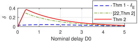
Figure 1: Comparison of the estimate $\delta_{\mathrm{E}}$ (4) derived from Theorem 1 with the admissible values of $\delta\in(0,D_{0})$ computed for $\kappa=0.2$ based on [22, Thm 2] and Theorem 5

For numerical simulations, we set the nominal value of the delay to $D_{0}=1\,\mathrm{s}$. In this case, Theorem 15 ensures the exponential stability of the closed-loop system with decay rate $\kappa=0.2$ for values of $\delta$ up to $\delta=0.260$. We set the initial condition $X_{0}(x)=-x(2L/3-x)(L-x)$ and the time-varying delay $D(t)=1+0.25\sin(3\pi t+\pi/4)$ which is of class $\mathcal{C}^{2}$ and is such that $|D(t)-D_{0}|\leq 0.25\leq 0.260$ and $|\dot{D}(t)|\leq 0.75\pi<+\infty$ for all $t\geq 0$. The transition time $t_{0}$ is taken as $t_{0}=0.5\,\mathrm{s}$ while the transition signal $\left.\varphi\right|_{[0,t_{0}]}$ is selected as the restriction over $[0,t_{0}]$ of the unique quintic polynomial function $f$ satisfying $f(0)=f^{\prime}(0)=f^{\prime\prime}(0)=f^{\prime}(t_{0})=f^{\prime\prime}(t_{0})=0$ and $f(t_{0})=1$. The employed numerical scheme relies on the discretization of the reaction-diffusion equation using its first 10 modes. The time domain evolution of the closed-loop system is depicted in Figs. 3-3. As expected from Theorem 15, both the system state and the control input converge to zero.

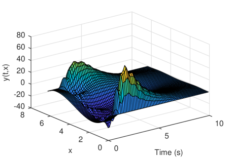
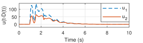
Figure 2: Time evolution of $y(t)$ for the closed-loop system

Figure 3: Delayed command effort $\tilde{u}(t)=u(t-D(t))$

5 Conclusion

This paper discussed first the use of predictor feedback for the stabilization of finite-dimensional LTI systems in the presence of an uncertain time-varying delay in the control input. By means of a Lyapunov-Krasovskii functional, it has been derived an LMI-based sufficient condition ensuring the exponential stability of the closed-loop system for small enough variations of the time-varying delay around its nominal value. Then, this result has been extended to the feedback stabilization of a class of diagonal infinite-dimensional boundary control systems.

References

• [1] Zvi Artstein. Linear systems with delayed controls: a reduction. IEEE Transactions on Automatic Control, 27(4):869–879, 1982.
• [2] Nikolaos Bekiaris-Liberis and Miroslav Krstic. Nonlinear control under delays that depend on delayed states. European Journal of Control, 19(5):389–398, 2013.
• [3] Nikolaos Bekiaris-Liberis and Miroslav Krstic. Robustness of nonlinear predictor feedback laws to time-and state-dependent delay perturbations. Automatica, 49(6):1576–1590, 2013.
• [4] Delphine Bresch-Pietri, Christophe Prieur, and Emmanuel Trélat. New formulation of predictors for finite-dimensional linear control systems with input delay. Systems & Control Letters, 113:9–16, 2018.
• [5] Xiushan Cai, Nikolaos Bekiaris-Liberis, and Miroslav Krstic. Input-to-state stability and inverse optimality of linear time-varying-delay predictor feedbacks. IEEE Transactions on Automatic Control, 63(1):233–240, 2018.
• [6] Ole Christensen et al. An Introduction to Frames and Riesz Bases. Springer, 2016.
• [7] R. F. Curtain and H. Zwart. An Introduction to Infinite-Dimensional Linear Systems Theory, volume 21. Springer Science & Business Media, 2012.
• [8] Emilia Fridman. A new Lyapunov technique for robust control of systems with uncertain non-small delays. IMA Journal of Mathematical Control and Information, 23(2):165–179, 2006.
• [9] Emilia Fridman. Tutorial on Lyapunov-based methods for time-delay systems. European Journal of Control, 20(6):271–283, 2014.
• [10] Iasson Karafyllis and Miroslav Krstic. Delay-robustness of linear predictor feedback without restriction on delay rate. Automatica, 49(6):1761–1767, 2013.
• [11] Vladimir Kolmanovskii and Anatolii Myshkis. Applied Theory of Functional Differential Equations, volume 85. Springer Science & Business Media, 2012.
• [12] Miroslav Krstic. Lyapunov tools for predictor feedbacks for delay systems: Inverse optimality and robustness to delay mismatch. Automatica, 44(11):2930–2935, 2008.
• [13] Miroslav Krstic. Control of an unstable reaction–diffusion pde with long input delay. Systems & Control Letters, 58(10-11):773–782, 2009.
• [14] Miroslav Krstic. Delay Compensation for Nonlinear, Adaptive, and PDE Systems. Springer, 2009.
• [15] Miroslav Krstic. Input delay compensation for forward complete and strict-feedforward nonlinear systems. IEEE Transactions on Automatic Control, 55(2):287–303, 2010.
• [16] Miroslav Krstic. Lyapunov stability of linear predictor feedback for time-varying input delay. IEEE Transactions on Automatic Control, 55(2):554–559, 2010.
• [17] Hugo Lhachemi and Christophe Prieur. Feedback stabilization of a class of diagonal infinite-dimensional systems with delay boundary control. arXiv preprint arXiv:1902.05086, 2019.
• [18] Hugo Lhachemi and Robert Shorten. ISS property with respect to boundary disturbances for a class of Riesz-spectral boundary control systems. Automatica, 109:108504, 2019.
• [19] Zhao-Yan Li, Bin Zhou, and Zongli Lin. On robustness of predictor feedback control of linear systems with input delays. Automatica, 50(5):1497–1506, 2014.
• [20] Christophe Prieur and Emmanuel Trélat. Feedback stabilization of a 1D linear reaction-diffusion equation with delay boundary control. IEEE Transactions on Automatic Control, 64(4):1415–1425, 2019.
• [21] David L Russell. Controllability and stabilizability theory for linear partial differential equations: recent progress and open questions. Siam Review, 20(4):639–739, 1978.
• [22] Anton Selivanov and Emilia Fridman. Predictor-based networked control under uncertain transmission delays. Automatica, 70:101–108, 2016.
• [23] Bin Zhou, Zongli Lin, and Guang-Ren Duan. Truncated predictor feedback for linear systems with long time-varying input delays. Automatica, 48(10):2387–2399, 2012.