Van der Waals Interactions in DFT using Wannier Functions without empirical parameters

Abstract

A new implementation is proposed for including van der Waals (vdW) interactions in Density Functional Theory (DFT) using the Maximally-Localized Wannier functions (MLWFs), which is free from empirical parameters. With respect to the previous DFT/vdW-WF2 method, in the present DFT/vdW-WF2-x approach, the empirical, short-range, damping function is replaced by an estimate of the Pauli exchange repulsion, also obtained by the MLWFs properties. Applications to systems contained in the popular S22 molecular database and to the case of an Ar atom interacting with graphite, and comparison with reference data, indicate that the new method, besides being more physically founded, also leads to a systematic improvement in the description of vdW-bonded systems.

I Introduction

Density Functional Theory (DFT) is a well-established computational approach to study the structural and electronic properties of condensed matter systems from first principles. Although current, approximated density functionals allow a quantitative description at much lower computational cost than other first principles methods, they failKohn to properly describe dispersion interactions. Dispersion forces originate from correlated charge oscillations in separate fragments of matter and the most important component is represented by the $R^{-6}$ van der Waals (vdW) interaction,london due to correlated instantaneous dipole fluctuations. These interactions play a fundamental role in determining the structure, stability, and function of a wide variety of systems, including molecules, clusters, proteins, nanostructered materials, molecular solids and liquids, and in adsorption processes of fragments weakly interacting with a substrate (”physisorbed”).

In the last few years a variety of practical methods have been proposed to make DFT calculations able to accurately describe vdW effects (for a review, see, for instance, refs. Riley, ; MRS, ; Klimes, ; Woods, ; Grimme2016, ; Hermann, ). In this respect, a family of such methods, all based on the Maximally Localized Wannier Functions (MLWFs),wannier has been developed, namely the original DFT/vdW-WF scheme,silvprl ; silvmetodo ; Mostofi DFT/vdW-WF2C3 (based on the London expression and taking into account the intrafragment overlap of the MLWFs), DFT/vdW-WF2sPRB2013 (including metal-screening corrections), and DFT/vdW-QHO-WFmyQHO (adopting the coupled Quantum Harmonic Oscillator model), successfully applied to a variety of systems: silvprl ; silvmetodo ; silvsurf ; CPL ; silvinter ; myQHO ; ambrosetti ; C3 ; Ar-Pb ; Costanzo ; Ambrosetti2013 ; PRB2013 ; Mostofi small molecules, water clusters, graphite and graphene, water layers interacting with graphite, interfacial water on semiconducting substrates, hydrogenated carbon nanotubes, molecular solids, the interaction of rare gases and small molecules with metal surfaces,…

In all these methods a certain degree of empiricism is present since the energetic vdW-correction term is multiplied by a short-range damping function, which is introduced not only to avoid the unphysical divergence of the vdW correction at small fragment separations, but also to eliminate double countings of correlation effects (in fact standard DFT approaches are able to describe short-range correlations). This damping function contains one or more empirical parameters which are typically set by a trial and error approach or/and are fitted using some reference database.

In the present paper we overcome the above limitation by presenting a new method, hereafter referred to as DFT/vdW-WF2-x, where the empirical, short-range, damping function is replaced by an estimate of the Pauli exchange repulsion, also obtained by the MLWFs properties. The new approach is successfully applied to the popular S22 benchmark setJurecka of weakly interacting molecules and also to the case of an Ar atom interacting with graphite. The results are compared with reference data and indicate that the new method leads to a systematic improvement in the description of vdW-bonded systems.

II Method

Here we describe and apply a new implementation of the DFT/vdW-WF2 method, introduced in ref. C3, and summarized below. Basically, the electronic charge partitioning is achieved using the Maximally-Localized Wannier Functions (MLWFs), which are obtained from a unitary transformation in the space of the occupied Bloch states, by minimizing the total spread functional:wannier

$$\Omega=\sum_{n}S^{2}_{n}=\sum_{n}\left(<w_{n}|r^{2}|w_{n}>-<w_{n}|\mathbf{r}|w_{n}>^{2}\right).$$ (1)

The localization properties of the MLWFs are of particular interest for the implementation of an efficient vdW correction scheme: in fact, the MLWFs represent a suitable basis set to evaluate orbital-orbital vdW interaction terms. In particular, if two interacting atoms, $A$ and $B$, are approximatedlondon by coupled harmonic oscillators, the vdW energy correction can be taken to be the change of the zero-point energy of the coupled oscillations as the atoms approach; if only a single excitation frequency is associated to each atom, $\omega_{A}$, $\omega_{B}$, then

$$E^{London}_{vdW}=-\frac{3e^{4}}{2m^{2}}\frac{Z_{A}Z_{B}}{\omega_{A}\omega_{B}(\omega_{A}+\omega_{B})}\frac{1}{R_{AB}^{6}}$$ (2)

where $Z_{A,B}$ is the total charge of A and B, and $R_{AB}$ is the distance between the two atoms ($e$ and $m$ are the electronic charge and mass). Now, adopting a simple classical theory of the atomic polarizability, the polarizability of an electronic shell of charge $eZ_{i}$ and mass $mZ_{i}$, tied to a heavy undeformable ion can be written as

$$\alpha_{i}\simeq\frac{Z_{i}e^{2}}{m\omega_{i}^{2}}\,.$$ (3)

Then, given the direct relation between polarizability and atomic volume,polvol we assume that $\alpha_{i}\sim\gamma S_{i}^{3}$, where $\gamma$ is a proportionality constant, so that the atomic volume is expressed in terms of the MLWF spread, $S_{i}$. Rewriting eq. (2) in terms of the quantities defined above, one obtains an explicit, simple expression for the $C_{6}$ vdW coefficient:

$$C_{6}^{AB}=\frac{3}{2}\frac{\sqrt{Z_{A}Z_{B}}S_{A}^{3}S_{B}^{3}\gamma^{3/2}}{(\sqrt{Z_{B}}S_{A}^{3/2}+\sqrt{Z_{A}}S_{B}^{3/2})}\,.$$ (4)

The constant $\gamma$ can then be set up by imposing that the exact value for the H atom polarizability ($\alpha_{H}=$4.5 a.u.) is obtained. This appears to be a physically sound choice since, in the H case, one knows the exact analytical spread, $S_{i}=S_{H}=\sqrt{3}$ a.u.

In order to achieve a better accuracy, one must properly deal with intrafragment MLWF overlap (we refer here to charge overlap, not to be confused with wave functions overlap): in fact, the method is strictly valid for nonoverlapping fragments only; now, while the overlap between the MLWFs relative to separated fragments is usually negligible for all the fragment separation distances of interest, the same is not true for the MLWFs belonging to the same fragment, which are often characterized by a significant overlap. This overlap affects the effective orbital volume, the polarizability, and the excitation frequency (see eq. (3)), thus leading to a quantitative effect on the value of the $C_{6}$ coefficient. We take into account the effective change in volume due to intrafragment MLWF overlap by introducing a suitable reduction factor $\xi$ obtained by interpolating between the limiting cases of fully overlapping and non-overlapping MLWFs. In particular, since in the DFT/vdW-WF2 method the $i$-th MLWF is approximated with a homogeneous charged sphere of radius $S_{i}$, then the overlap among neighboring MLWFs can be evaluated as the geometrical overlap among neighboring spheres. To derive the correct volume reweighting factor for dealing with overlap effects, we first consider the limiting case of two pairs (one for each fragment) of completely overlapping MLWFs, which would be, for instance, applicable to two interacting He atoms if each MLWF just describes the density distribution of a single electron; then we can evaluate a single $C_{6}$ coefficient using eq. (4) with $Z_{A,B}=2$, so that:

$$C_{6}^{AB}=\frac{3}{2}\frac{\sqrt{2}S_{A}^{3}S_{B}^{3}\gamma^{3/2}}{(S_{A}^{3/2}+S_{B}^{3/2})}.$$ (5)

Alternatively, the same expression can be obtained by considering the sum of 4 identical pairwise contributions (with $Z=1$), by introducing a modification of the effective volume in such a way to take the overlap into account and make the global interfragment $C_{6}$ coefficient equivalent to that in eq. (5). This is clearly accomplished by replacing $S_{i}^{3}$ in eq. (4) with $\xi S_{i}^{3}$, where $\xi=1/2$. This procedure can be easily generalized to multiple overlaps, by weighting the overlapping volume with the factor $n^{-1}$, where $n$ is the number of overlapping MLWFs. Finally, by extending the approach to partial overlaps, we define the free volume of a set of MLWFs belonging to a given fragment (in practice three-dimensional integrals are evaluated by numerical sums introducing a suitable mesh in real space) as:

$$V_{free}=\int d\mathbf{r}\,w_{free}(\mathbf{r})\simeq\Delta r\sum_{l}w_{free}(\mathbf{r}_{l})$$ (6)

where $w_{free}(\mathbf{r}_{l})$ is equal to 1 if $|\mathbf{r}_{l}-\mathbf{r}_{i}|<S_{i}$ for at least one of the fragment MLWFs, and is 0 otherwise.

The corresponding effective volume is instead given by

$$V_{eff}=\int d\mathbf{r}\,w_{eff}(\mathbf{r})\simeq\Delta r\sum_{l}w_{eff}(\mathbf{r}_{l})\,,$$ (7)

where the new weighting function is defined as $w_{eff}(\mathbf{r}_{l})=w_{free}(\mathbf{r}_{l})\cdot n_{w}(\mathbf{r}_{l})^{-1}$, with $n_{w}(\mathbf{r}_{l})$ that is equal to the number of MLWFs contemporarily satisfying the relation $|\mathbf{r}_{l}-\mathbf{r}_{i}|<S_{i}$. Therefore, the non overlapping portions of the spheres (in practice the corresponding mesh points) will be associated to a weight factor 1, those belonging to two spheres to a $1/2$ factor, and, in general, those belonging to $n$ spheres to a $1/n$ factor. The average ratio between the effective volume and the free volume ($V_{eff}/V_{free}$) is then assigned to the factor $\xi$, appearing in eq. (8). Although in principle the correction factor $\xi$ must be evaluated for each MLWF and the calculations must be repeated at different fragment-fragment separations, our tests show that, in practice, if the fragments are rather homogeneous all the $\xi$ factors are very similar, and if the spreads of the MLWFs do not change significantly in the range of the interfragment distances of interest, the $\xi$’s remain essentially constant; clearly, exploiting this behavior leads to a significant reduction in the computational cost of accounting for the intrafragment overlap. We therefore arrive at the following expression for the $C_{6}$ coefficient:

$$C_{6}^{AB}=\frac{3}{2}\frac{\sqrt{Z_{A}Z_{B}}\xi_{A}S_{A}^{3}\xi_{B}S_{B}^{3}\gamma^{3/2}}{(\sqrt{Z_{B}\xi_{A}}S_{A}^{3/2}+\sqrt{Z_{A}\xi_{B}}S_{B}^{3/2})}\,,$$ (8)

where $\xi_{A,B}$ represents the ratio between the effective and the free volume associated to the $A$-th and $B$-th MLWF. The need for a proper treatment of overlap effects has been also pointed out by Andrinopoulos et al.,Mostofi who however applied a correction only to very closely centred WFCs.

Finally, in the original DFT/vdW-WF2 method, the vdW interaction energy was computed as:

$$E_{vdW}=-\sum_{i<j}f(R_{ij})\frac{C_{6}^{ij}}{R^{6}_{ij}}=-\sum_{i<j}\frac{C_{6}^{ij}}{R^{6}_{ij}}+\sum_{i<j}\left(1-f(R_{ij})\right)\frac{C_{6}^{ij}}{R^{6}_{ij}}\,\,,$$ (9)

where $f(R_{ij})$ is a short-range damping function, which is introduced not only to avoid the unphysical divergence of the vdW correction at small fragment separations, but also to eliminate double countings of correlation effects (in fact standard DFT approaches are able to describe short-range correlations); it is defined as:

$$f(R_{ij})=\frac{1}{1+e^{-a(R_{ij}/R_{s}-1)}}\,.$$ (10)

The parameter $R_{s}$ represents the sum of the vdW radii $R_{s}=R_{i}^{vdW}+R_{j}^{vdW}$, with (by adopting the same criterion chosen above for the $\gamma$ parameter)

$$R_{i}^{vdW}=R_{H}^{vdW}\frac{S_{i}}{\sqrt{3}}\,\,,$$ (11)

where $R_{H}^{vdW}$ is the literatureBondi (1.20 Å) vdW radius of the H atom, and, following Grimme et al.,Grimme $a\simeq 20$. Although $a$ is the only ad-hoc parameter of the method, while all the others are only determined by the basic information given by the MLWFs (that is from first principles calculations) and in many applications the results are only mildly dependent on the particular value of $a$, nonetheless, this parameter, together with the choice of a specific form of the above damping function, clearly imply a certain degree of empiricism.

In order to overcome this limitation, we propose to improve the approach by replacing the somehow artificial, short-range damping function by a term that directly measures the quantum mechanical Pauli exchange repulsion between electronic orbitals and can be entirely expressed in terms of the MLWFs properties, without the need of introducing empirical parameters. Following ref. Fedorov, , using the dipole approximation for the Coulomb interaction, the exchange integral, for two closed electronic shells with total zero spin, is simply given by:

$$J_{ex}=\frac{q^{2}O}{2R}\,,$$ (12)

where $q$ indicates the electronic charge of each electronic shell and $O$ is the overlap integral between the electronic shells, separated by $R$. In our specific case, assuming that an electronic orbital is described by the wave function relative to a quantum harmonic oscillator:

$$\psi_{A}(r)=\left(\frac{3}{2\pi}\right)^{3/4}\frac{1}{S_{A}^{3/2}}\,e^{-\left(\frac{3r^{2}}{4S_{A}^{2}}\right)}\;\,,$$ (13)

where $S_{A}$ is the spread of the corresponding MLWF, then one can easily obtain that :

$$O_{AB}=8\frac{S_{A}^{3}S_{B}^{3}}{(S_{A}^{2}+S_{B}^{2})^{3}}\,e^{-\left(\frac{3}{2}\frac{R_{AB}^{2}}{S_{A}^{2}+S_{B}^{2}}\right)}\;\,.$$ (14)

Then, the exchange integral can be expressed in terms of the MLWFs spreads as :

$$J_{ex}^{AB}(R_{AB})=\frac{q^{2}O_{AB}}{2R_{AB}}=4\frac{q^{2}}{R_{AB}}\frac{S_{A}^{3}S_{B}^{3}}{(S_{A}^{2}+S_{B}^{2})^{3}}\,e^{-\left(\frac{3}{2}\frac{R_{AB}^{2}}{S_{A}^{2}+S_{B}^{2}}\right)}\;\,.$$ (15)

Therefore, in this new DFT/vdW-WF2-x version of the method, the vdW interaction energy is computed as:

$$E_{vdW}=-\sum_{i<j}\frac{C_{6}^{ij}}{R^{6}_{ij}}+\sum_{i<j}J_{ex}^{ij}(R_{ij})\;\,.$$ (16)

In this way the vdW energy correction is evaluated as the sum of two terms, both expressed in terms of the MLWfs spreads, thus making explicit the direct connection between attractive and repulsive parts of the vdW interaction.Fedorov

Of course there are very weakly bonded systems, entirely dominated by vdW effects, where the repulsive term is not relevant for determining the equilibrium complex configuration. For instance, in the Ar-dimer case, DFT/vdW-WF2 and DFT/vdW-WF2-x predict the same equilibrium Ar-Ar distance and the same binding energy (within 0.1 meV). However, in most cases, a proper treatment of short-range repulsion is crucial to correctly describe the minimum, equilibrium configuration.

The calculations have been performed with both the CPMDCPMD and the Quantum-ESPRESSO ab initio packageESPRESSO (in the latter case the MLWFs have been generated as a post-processing calculation using the WanT packageWanT ), using norm-conserving or ultrasoft pseudopotentials to describe the electron-ion interactions and taking mainly PBEPBE as the reference, Generalized Gradient Approximation (GGA) DFT functional, although test calculations have been also carried out using the BLYPBLYP GGA functional. PBE and BLYP are chosen because they represent two of the most popular GGA functionals for standard DFT simulations of condensed-matter systems.

III Results and Discussion

In order to assess the accuracy of the DFT/vdW-WF2-x method we first consider the S22 database of intermolecular interactions,Jurecka a widely used benchmark database, consisting of weakly interacting molecules (a set of 22 weakly interacting dimers mostly of biological importance), with reference binding energies calculated by a number of different groups using high-level quantum chemical methods. In particular, we use the basis-set extrapolated CCSD(T) binding energies calculated by Takatani et al.Takatani These binding energies are presumed to have an accuracy of about 0.1 kcal/mol (1% relative error). Calculations have been performed using the same technical parameters adopted in ref. myQHO, .

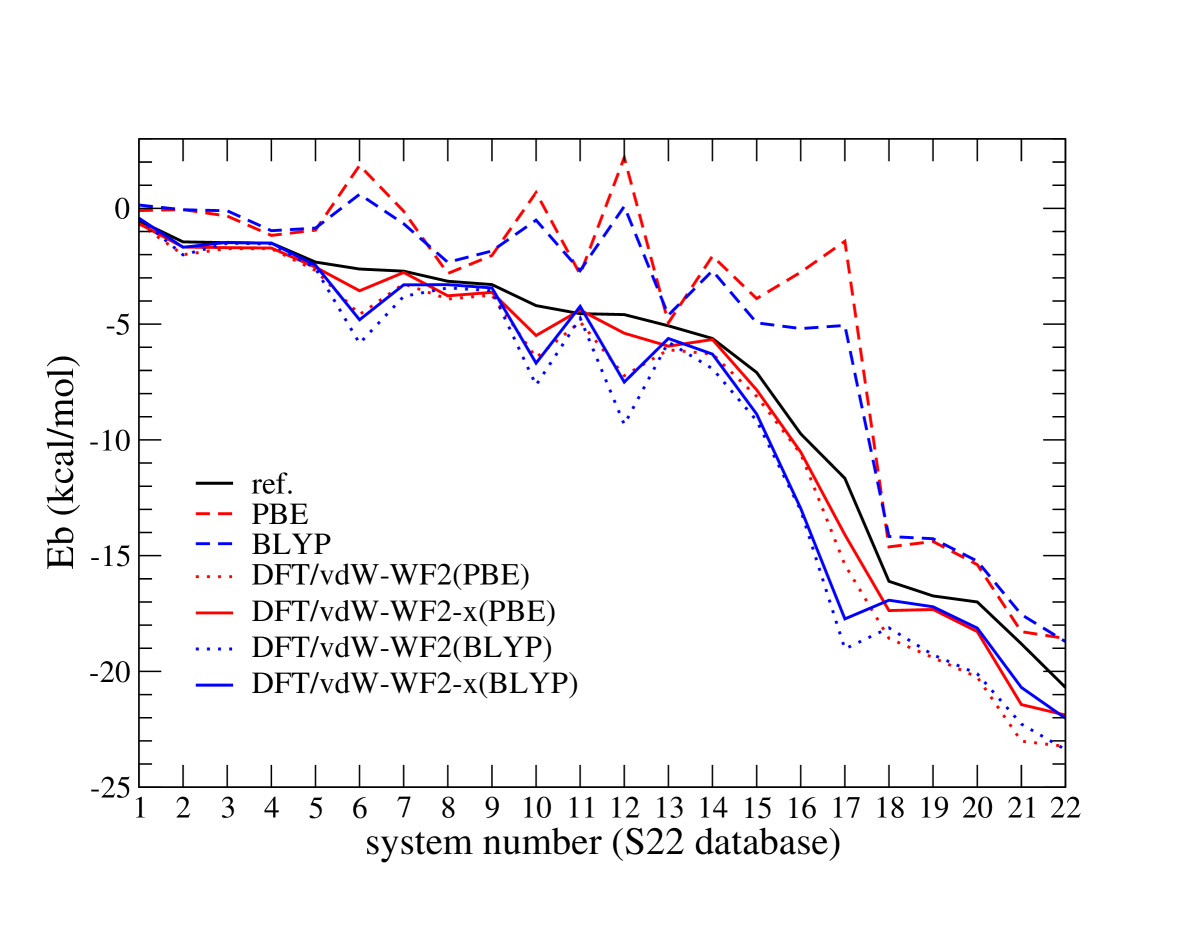
Figure 1: Binding energy for all the 22 complexes contained in the S22 database, listed (for the sake of better visibility) in the order of increasing (absolute) value of the reference binding energy using different functionals.

Table I summarizes the results of our calculations on the S22 database, at the DFT/vdW-WF2-x level, considering PBE (DFT/vdW-WF2-x(PBE)) or BLYP (DFT/vdW-WF2-x(BLYP)) as the reference DFT functional, compared to those obtained by other vdW-corrected DFT schemes, namely DFT/vdW-WF2,C3 vdW-DF,Dion ; Langreth07 vdW-DF2,Lee-bis VV10Vydrov and rVV10Sabatini (the revised, computationally much more efficient version of the VV10 method), PBE+TS-vdW,TS and PBE+MBD.Tkatchenko12 For the sake of completeness we also report data relative to the semiempirical PBE-D3Grimme approach and to the bare, non-vdW-corrected, PBE and BLYP functionals. In Table II, the performance of different schemes is illustrated by separately considering Hydrogen-bonded, dispersion, and mixed complexes, while Fig. 1 reports the behavior of the binding energy for all the 22 complexes contained in the S22 database, listed (for the sake of better visibility) in the order of increasing (absolute) value of the reference, binding energy. As expected, considering the whole S22 database, pure PBE and BLYP perform poorly and a substantial improvement can be obtained by vdW-corrected approaches. More importantly, the performances of the new DFT/vdW-WF2-x scheme are clearly better than those of the previous DFT/vdW-WF2 method. In particular, the general tendency of DFT/vdW-WF2 to overbind is considerably reduced by DFT/vdW-WF2-x. Interestingly, with DFT/vdW-WF2-x(PBE) the mean absolute error (MAE), 0.78 kcal/mol, is well below the so-called ”chemical accuracy” threshold of 1 kcal/mol, required to attribute a genuine quantitative character to the predictions of an ab initio scheme. Moreover, DFT/vdW-WF2-x(PBE) performs better than the more sophisticated vdW-DF and vdW-DF2 methods, based on the use of a nonlocal expression for the correlation energy-term, is comparable, as far as the S22 database is concerned to PBE-D3, and its performances are only inferior to those of the rVV10, VV10, PBE+TS-vdW, and PBE+MBD schemes, which are among the most accurate vdW-corrected DFT approaches for noncovalently bound complexes.Sabatini ; Tkatchenko12 As can be seen, looking at Table II, DFT/vdW-WF2-x(PBE) turns out to be better than DFT/vdW-WF2-x(BLYP) for both dispersion-dominated and mixed complexes, while instead the opposite is true for Hydrogen-bonded complexes.

In order to test the applicability of the present DFT/vdW-WF2-x method also to a representative of extended systems, which of course is of particular interest because, in this case, high-quality chemistry methods are typically too computationally demanding, we considered the adsorption of a single Ar atom on graphite, that is a typical physisorption process. Calculations have been performed using the same DFT approach followed in ref. ambr, and considering the adsorption on the more favored hollow site only. Table III reports the binding energy, E_b, and equilibrium distance R, for an Ar atom adsorbed on graphite, while in Fig. 2 the corresponding binding energy curves are shown. Data obtained at the PBE, DFT/vdW-WF2(PBE), and DFT/vdW-WF2-x(PBE) level are compared to reference theoretical and experimental estimates. Theoretical values were obtained by Tkatchenko et al.,Tkatchenko with a DFT-vdW corrected scheme based on a semiempirical dispersion calibrated atom-centered potential, and by Bichoutskaia and Pyper, with the inclusion of Axilord-Teller dispersion interactions.Ar As can be seen, the pure PBE functional largely underbinds while vdW-corrected schemes predict a much stronger Ar-graphite interaction with the formation of a clear minimum in the binding energy curve at a shorter equilibrium distance. At relatively large Ar-graphite distances, as expected, the DFT/vdW-WF2-x(PBE) curve approaches the DFT/vdW-WF2(PBE) one, since the repulsive term becomes irrelevant. However, near the equilibrium position, which is just determined by an interplay between attractive vdW interaction and repulsion, the differences in the binding energies are significant, with DFT/vdW-WF2-x(PBE) which represents an evident improvement compared to DFT/vdW-WF2(PBE), and, in line with what previously observed in the application to the S22 database, leads to a reduction of the binding-energy estimate, thus showing that the effect of the repulsive term is more relevant. This can be seen more explicitly looking at Fig. 3, where the repulsive contribution (see eq. (9)) of the DFT/vdW-WF2(PBE) method, $\sum_{i<j}\left(1-f(R_{ij})\right)\frac{C_{6}^{ij}}{R^{6}_{ij}}$, is compared to that (see eq. (16)) of DFT/vdW-WF2-x(PBE), $\sum_{i<j}J_{ex}^{ij}(R_{ij})$. Clearly, the repulsive term vanishes for Ar-graphite distances larger than 4 Å, however, around the equilibrium distance (and at shorter distances), it is much more substantial in the DFT/vdW-WF2-x(PBE) approach than in DFT/vdW-WF2(PBE).

The DFT/vdW-WF2-x(PBE) binding energy (-115 meV) is very close to the values reported by Tkatchenko et al.Tkatchenko (-116 meV) and Bichoutskaia and PyperAr (-111 meV). Moreover, this value is also compatible with one of the few experimental estimates, represented by the measurement of the latent heat of condensation relative to the adsorption of an Ar monolayer on graphite: -119 $\pm$ 2 meV/atom.Shaw It is also close to the ”best estimate” (obtained from a combination of experimental and theoretical, mainly semiempirically-based, data) reported in the milestone review paper by Vidali et al.,Vidali that is -99 $\pm$ 4 meV. Our DFT/vdW-WF2-x(PBE) computed Ar-graphite equilibrium distance is instead somehow larger than that reported in other theoretical studiesAr ; Tkatchenko (3.3 Å), and also than the ”best estimate” by Vidali et al.Vidali of 3.1 $\pm$ 0.1 Å (and an old experimental measurement of 3.2 $\pm$ 0.1 Å, see ref. Vidali, ). However one sould observe that an accurate estimate of this quantity is more difficult due to the relatively shallow potential energy curve of this system.

IV Conclusions

In summary, we have presented a new method for including van der Waals (vdW) interactions in Density Functional Theory using the MLWFs, which is free from empirical parameters. With respect to the previous DFT/vdW-WF2 method, in the present DFT/vdW-WF2-x approach, the empirical, short-range, damping function is replaced by an estimate of the Pauli exchange repulsion, also obtained by the MLWFs properties. Applications to systems contained in the popular S22 molecular database and to the case of an Ar atom interacting with graphite, and comparison with reference data, indicate that the new method, besides being more physically founded, also leads to a systematic improvement in the description of vdW-bonded systems.

V Acknowledgements

We acknowledge funding from Fondazione Cariparo, Progetti di Eccellenza 2017, relative to the project: ”Engineering van der Waals Interactions: Innovative paradigm for the control of Nanoscale Phenomena”.

Table 1: Performance of different schemes on the S22 database of intermolecular interactions. The errors are measured with respect to basis-set extrapolated CCSD(T) calculations of Takatani et al.Takatani Mean absolute relative errors (MARE in %) and mean absolute errors (MAE in kcal/mol, and, in parenthesis, in meV) are reported.

method	MARE	MAE
PBE	55.5	2.56[111.0]
DFT/vdW-WF2(PBE)	24.4	1.50 [65.1]
DFT/vdW-WF2-x(PBE)	13.4	0.78 [33.8]
BLYP	52.9	2.24 [97.1]
DFT/vdW-WF2(BLYP)	31.1	1.94 [84.1]
DFT/vdW-WF2-x(BLYP)	20.5	1.24 [53.8]
vdW-DFa	17.0	1.22 [52.9]
vdW-DF2b	14.7	0.94 [40.8]
VV10b	4.4	0.31 [13.4]
rVV10c	4.3	0.30 [13.0]
PBE+TS-vdWd,e	10.3	0.32 [13.9]
PBE+MBDd	6.2	0.26 [11.3]
PBE-D3c,f	11.4	0.50 [21.7]

Table 2: Performance of different schemes on the S22 database of intermolecular interactions, by separately considering Hydrogen-bonded, dispersion, and mixed complexes. The errors are measured with respect to basis-set extrapolated CCSD(T) calculations of Takatani et al.Takatani Mean absolute relative errors (MARE in %) and mean absolute errors (MAE in kcal/mol, and, in parenthesis, in meV) are reported.

method	MARE	MAE
Hydrogen-bonded complexes:
PBE	8.4	1.22 [52.9]
DFT/vdW-WF2(PBE)	18.5	2.42[105.0]
DFT/vdW-WF2-x(PBE)	10.8	1.21 [52.5]
BLYP	12.6	1.53 [66.4]
DFT/vdW-WF2(BLYP)	14.3	2.11 [91.5]
DFT/vdW-WF2-x(BLYP)	6.6	0.90 [39.0]
Dispersion complexes:
PBE	106.4	4.54[196.9]
DFT/vdW-WF2(PBE)	38.4	1.55 [67.2]
DFT/vdW-WF2-x(PBE)	21.0	0.85 [36.9]
BLYP	91.6	3.27[141.8]
DFT/vdW-WF2(BLYP)	58.1	2.84[123.2]
DFT/vdW-WF2-x(BLYP)	41.0	2.15 [93.2]
Mixed complexes:
PBE	51.6	2.00 [86.7]
DFT/vdW-WF2(PBE)	14.3	0.52 [22.6]
DFT/vdW-WF2-x(PBE)	7.2	0.25 [10.8]
BLYP	48.9	1.78 [77.2]
DFT/vdW-WF2(BLYP)	17.0	0.75 [32.5]
DFT/vdW-WF2-x(BLYP)	11.0	0.52 [22.6]

Table 3: Binding energy, E_b, and equilibrium distance R, for an Ar atom adsorbed on graphite.

method	Eb (meV)	R (Å)
PBE	-12	4.0
DFT/vdW-WF2(PBE)	-145	3.3
DFT/vdW-WF2-x(PBE)	-115	3.5
ref.theorya	-116	3.3
ref.theorya	-111	3.3
ref.expt.c	-99 $\pm$ 4	3.0 $\pm$ 0.1
ref.expt.d	—	3.2 $\pm$ 0.1

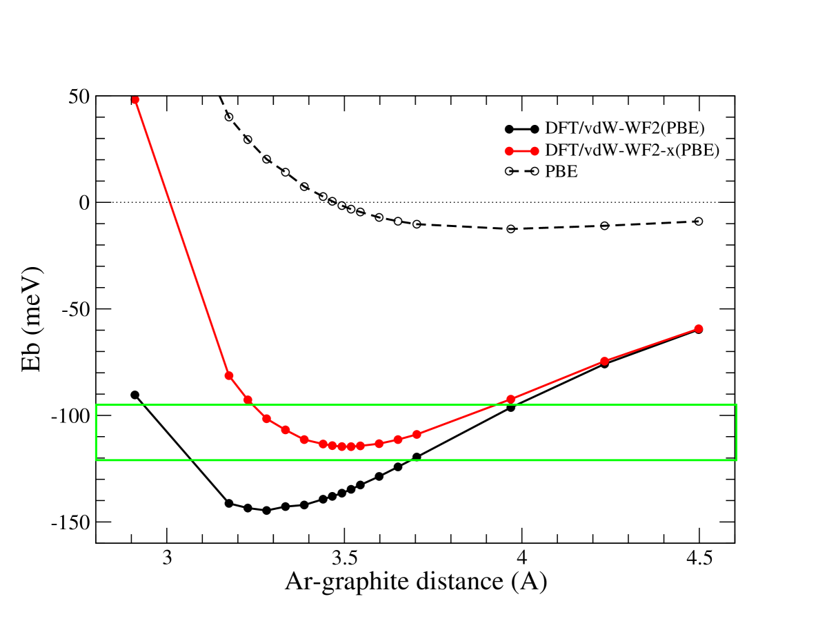
Figure 2: Binding energy of Ar on graphite. The horizontal green box denotes the binding-energy range corresponding to the theoretical and experimental estimates (see Table III).

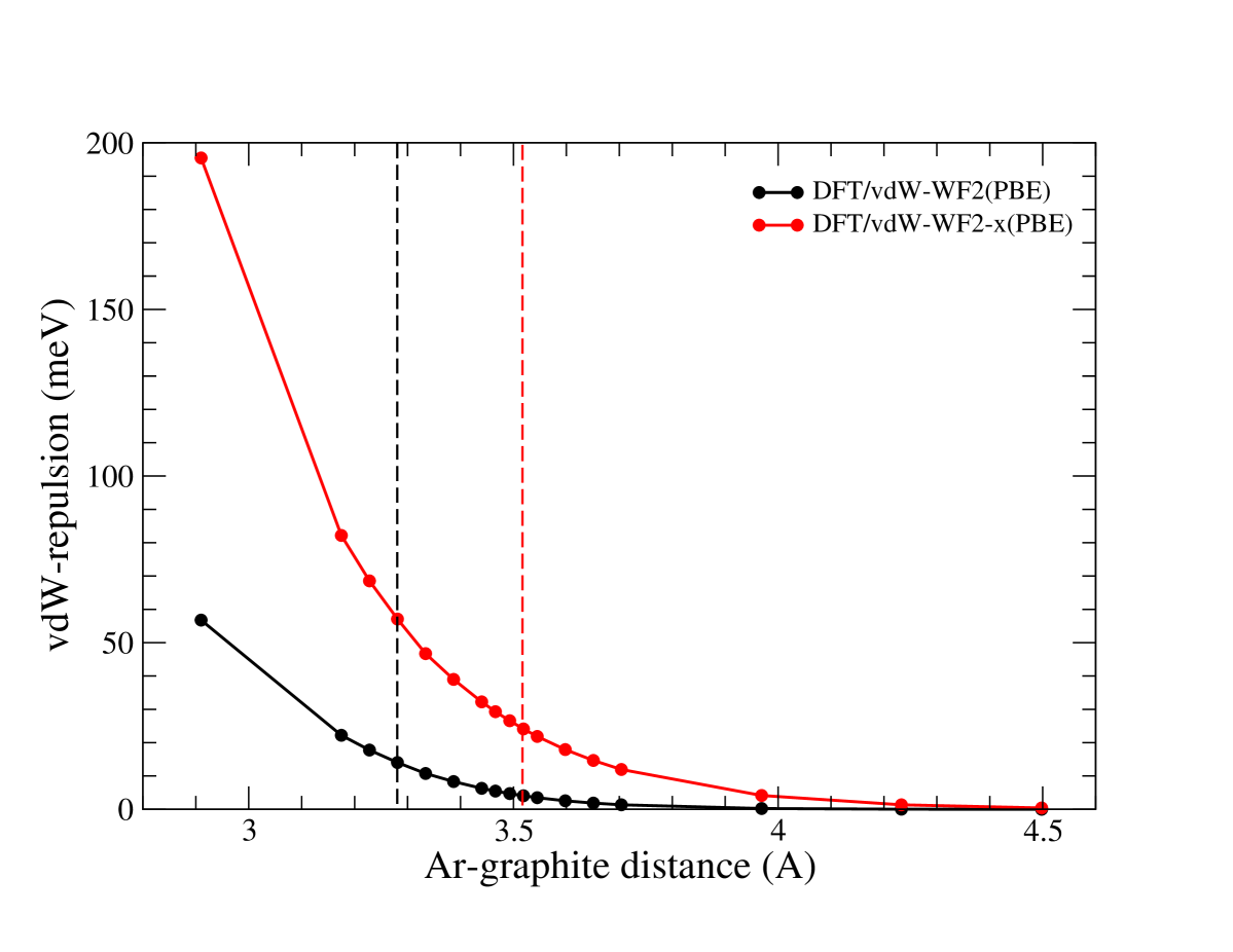
Figure 3: Repulsive component of the vdW correction (see text) for Ar on graphite. The vertical dashed lines indicate the positions of the equilibrium distances.

References

- (1) See, for instance, W. Kohn, D. E. Makarov, Phys. Rev. Lett. 80, 4153 (1998).
- (2) R. Eisenhitz and F. London, Z. Phys. 60, 491 (1930).
- (3) K. E. Riley, M. Pitoňák, P. Jurečka, P. Hobza, Chem. Rev. 110, 5023 (2010).
- (4) A. Tkatchenko, L. Romaner, O. T. Hofmann, E. Zojer, C. Ambrosch-Draxl, and M. Scheffler, MRS Bulletin, 35, 435 (2010).
- (5) J. Klimeš, A. Michaelides, J. Chem. Phys. 137, 120901 (2012).
- (6) L. M. Woods, D. A. R. Dalvit, A. Tkatchenko, P. Rodriguez-Lopez, A. W. Rodriguez, R. Podgornik, Rev. Mod. Phys. 88, 045003 (2016).
- (7) S. Grimme, A. Hansen, J. G. Brandenburg, C. Bannwarth, Chem. Rev. 116, 5105 (2016).
- (8) J. Hermann, R. A. DiStasio Jr., A. Tkatchenko, Chem. Rev. 117 (2017) 4714.
- (9) N. Marzari and D. Vanderbilt, Phys. Rev. B 56, 12847 (1997).
- (10) P. L. Silvestrelli, Phys. Rev. Lett 100, 053002 (2008).
- (11) P. L. Silvestrelli, J. Phys. Chem. A 113, 5224 (2009).
- (12) L. Andrinopoulos, N. D. M. Hine, A. A. Mostofi, J. Chem. Phys. 135, 154105 (2011).
- (13) A. Ambrosetti, P. L. Silvestrelli, Phys. Rev. B 85, 073101 (2012); Phys. Rev. B 87, 039902 (2013).
- (14) P. L. Silvestrelli and A. Ambrosetti, Phys. Rev. B 87, 075401 (2013).
- (15) P. L. Silvestrelli, J. Chem. Phys. 139, 054106 (2013).
- (16) P. L. Silvestrelli, K. Benyahia, S. Grubisic, F. Ancilotto, and F. Toigo, J. Chem. Phys. 130, 074702 (2009).
- (17) P. L. Silvestrelli, Chem. Phys. Lett. 475, 285 (2009).
- (18) P. L. Silvestrelli, F. Toigo, F. Ancilotto, J. Phys. Chem. C 113, 17124 (2009).
- (19) A. Ambrosetti, P. L. Silvestrelli, J. Phys. Chem. C 115, 3695 (2011).
- (20) P. L. Silvestrelli, A. Ambrosetti, S. Grubisiĉ, and F. Ancilotto, Phys. Rev. B 85, 165405 (2012).
- (21) F. Costanzo, P. L. Silvestrelli, Francesco Ancilotto, J. Chem. Theory Comp. 8, 1288 (2012).
- (22) A. Ambrosetti, F. Ancilotto, P. L. Silvestrelli, J. Phys. Chem. C 117, 321 (2013).
- (23) P. Jurečka, J. Šponer, J. Černy, P. Hobza, Phys. Chem. Chem. Phys. 8, 1985 (2006).
- (24) T. Brink, J. S. Murray, P. Politzer, J. Chem. Phys. 98, 4305 (1993).
- (25) A. Bondi, J. Phys. Chem. 68, 441 (1964).
- (26) S. Grimme, J. Antony, T. Schwabe, C. Mück-Lichtenfeld, Org. Biomol. Chem. 5, 741 (2007); S. Grimme, J. Antony, S. Ehrlich, H. Krieg, J. Chem. Phys. 132, 154104 (2010).
- (27) D. V. Fedorov, M. Sadhukhan, M. Stöd, A. Tkatchenko, Phys. Rev. Lett. 121, 183401 (2018).
- (28) CPMD, http://www.cpmd.org/, Copyright IBM Corp 1990-2019, Copyright MPI für Festkörperforschung Stuttgart 1997-2001.
- (29) P. Giannozzi, S. Baroni, N. Bonini, M. Calandra, R. Car, C. Cavazzoni, D. Ceresoli, G. L. Chiarotti, M. Cococcioni, I. Dabo, A. Dal Corso, S. Fabris, G. Fratesi, S. de Gironcoli, R. Gebauer, U. Gerstmann, C. Gougoussis, A. Kokalj, M. Lazzeri, L. Martin-Samos, N. Marzari, F. Mauri, R. Mazzarello, S. Paolini, A. Pasquarello, L. Paulatto, C. Sbraccia, S. Scandolo, G. Sclauzero, A. P. Seitsonen, A. Smogunov, P. Umari, R. M. Wentzcovitch, J.Phys.: Condens. Matter 21, 395502 (2009); http://arxiv.org/abs/0906.2569.
- (30) WanT code by A. Ferretti, B. Bonferroni, A. Calzolari, and M. Buongiorno Nardelli, (http://www.wannier-transport.org). See also: A. Calzolari, N. Marzari, I. Souza and M. Buongiorno Nardelli, Phys. Rev. B 69, 035108 (2004).
- (31) J.P. Perdew, K. Burke, M. Ernzerhof, Phys. Rev. Lett. 77, 3865 (1996).
- (32) A. D. Becke, Phys. Rev. A 38, 3098 (1988); C. Lee, W. Yang, and R. C. Parr, Phys. Rev. B 37, 785 (1988).
- (33) T. Takatani, E. G. Hohenstein, M. Malagoli, M. S. Marshall, C. D. Sherril, J. Chem. Phys. 132, 144104 (2010).
- (34) M. Dion, H. Rydberg, E. Schröder, D. C. Langreth, B. I. Lundqvist, Phys. Rev. Lett. 92, 246401 (2004); G. Roman-Perez, J. M. Soler, Phys. Rev. Lett. 103, 096102 (2009).
- (35) T. Thonhauser, V. R. Cooper, S. Li, A. Puzder, P. Hyldgaard, D. C. Langreth, Phys. Rev. B 76, 125112 (2007).
- (36) K. Lee, É. D. Murray, L. Kong, B. I. Lundqvist, and D. C. Langreth, Phys. Rev. B 82, 081101(R) (2010).
- (37) O. A. Vydrov, T. van Voorhis, J. Chem. Phys. 133, 244103 (2010).
- (38) R. Sabatini, T. Gorni, S. de Gironcoli, Phys. Rev. B 87, 041108(R) (2013).
- (39) A. Tkatchenko, M. Scheffler, Phys. Rev. Lett. 102, 073005 (2009).
- (40) A. Tkatchenko, R. A. Di Stasio, R. Car, M. Scheffler, Phys. Rev. Lett. 108, 236402 (2012).
- (41) A. Ambrosetti, P. L. Silvestrelli, J. Phys. Chem. C 115, 1695 (2011).
- (42) A. Tkatchenko, O. A. von Lilienfeld, Phys. Rev. B 73, 153406 (2006).
- (43) E. Bichoutskaia, N. C. Pyper, J. Chem. Phys. 128, 024709 (2008).
- (44) C. G. Shaw, S. C. Fain Jr., Surf. Sci. 91, L1 (1980).
- (45) G. Vidali, G. Ihm, H. Y. Kim, M. W. Cole, Surf. Sci. Rep. 12, 133 (1991).
- (46) V. R. Cooper, Phys. Rev. B 81, 161104(R) (2010).
- (47) R. A. Di Stasio Jr., O. A. von Lilienfeld, A. Tkatchenko, PNAS 109, 14791 (2012).
- (48) Chemistry and Physics of Solid Surfaces IV, edited by R. Vanselow and R. Howe, Springer Series in Chemical Physics (1982).