Entropies for Coupled Harmonic Oscillators and Temperature

Ahmed Jellal^a and Abdeldjalil Merdaci^b

^aLaboratory of Theoretical Physics, Faculty of Sciences, Chouaïb Doukkali University,

PO Box 20, 24000 El Jadida, Morocco

^bPhysics Department, College of Science, King Faisal University,
PO Box 380, Alahsa 31982, Saudi Arabia

We study two entropies of a system composed of two coupled harmonic oscillators which is brought to a canonical thermal equilibrium with a heat-bath at temperature $T$. Using the purity function, we explicitly determine the Rényi and van Newmon entropies in terms of different physical parameters. We will numerically analyze these two entropies under suitable conditions and show their relevance.

PACS numbers: 03.65.Ud, 03.65.-w, 03.67.-a

Keywords: Two coupled harmonic oscillator, path integral, density matrix, thermal wavefunction, entropies.

1 Introduction

The study of information carried by signals attracted several researchers because of its relevance to telecommunications. Historically, the first theory on the subject going back to Shannon [1] who formulated a mathematical tool based on the probability aspects of events and initiated a new field of research called actually information theory. Indeed, Shannon showed that the amount of information carried by a sequence of events $p_{1},p_{2},\cdots$ can be described by the entropy $S(p)=-K\sum_{i=1}^{N}p_{i}\ln p_{i}$ with $K$ a positive constant. It has to verify three conditions on: (i) $S(P)$ should be continuous in $p_{i}$, (ii) $S(p)$ should be a monotonic increasing function of $N$ when all $p_{i}=\frac{1}{N}$ are equally probably, (iii) $S(p)$ should be additive. Later on, the Shannon theory has been extended to many measures of information or entropy. One of them is due to Rényi [2], which he was able to extend the Shannon entropy to a continuous family of entropies of the forms $S_{q}=\frac{\ln{\rm Tr}\rho^{q}}{1-q}$, with a single parameter $q>1$. The entropies $S_{q}$ cover also that of the von Neumann $S_{1}$, which can be recovered by requiring the limit $q\longrightarrow 1$.

For a many-body quantum system composed of two subsystems $(A,B)$, the bipartite entanglement between subsystems is described by a state $\Psi$ of the Hilbert space ${\cal{H}}={\cal{H}}_{A}\otimes{\cal{H}}_{B}$. The corresponding the reduced density matrix $\rho_{A}={\rm Tr}_{B}\left(\rho_{AB}\right)$ is obtained by tracing out the density matrix of the full system $\rho_{AB}=|\Psi\rangle\langle\Psi|$. Noting that if $\rho_{AB}$ is a pure state then it suffices to use the von Neumann entropy in order to measure the amount of the entanglement. However, the Rényi entropy has further importance because it provides complete information about the eigenvalue distribution of the reduced density matrix $\rho_{A}$ and therefore completely characterizes the entanglement in an overall pure, bipartite state [3, 4]. In fact, the entanglement encodes the amount of non-classical information shared between complementary parts of an extended quantum state. For a pure state described by density matrix, it can be quantified via the Rényi entanglement entropies.

In studying the entanglement in a quantum system, we have proposed a new approach [5] to explicitly determine the purity function for the whole energy spectrum rather than the ground state as mostly used in the literature. This was done by choosing the two coupled harmonic oscillators as system and using the path integral technique as tools to deal with our issues. Among the obtained results, we have derived a thermal wavefunction depending on temperature that plied a crucial role in discussing different properties of our system. To prove the validity of our approach, we have showed that our results reduce to the standard case describing the quantum system in the ground state at absolute zero temperature. This result has been obtained in our previous work dealing with the entanglement in coupled harmonic oscillators studied using a unitary transformation [6].

We deal with other issues related to the thermal wavefunction obtained in our work [5]. More precisely, we study the two entropies corresponding to two coupled harmonic oscillators, which is brought to a canonical thermal equilibrium with a heat-bath at temperature $T$. Indeed, we use our purity function to explicitly determine the Rényi and von Neumann entropies as function of the temperature parameter introduced through the path integral method. In fact, we show that the von Neumann entropy can be derived as limiting case $q\longrightarrow 1$ of that of Rényi of order $q$. To highlight our results we present different density plots of both entropies and show their basic properties. These will be done by choosing different configurations of the coupling parameter $\eta$, mixing angle $\theta$ and temperature $\beta=\frac{1}{k_{B}T}$.

The present paper is organized as follows. In section 2, we review our main results [5] needed to deal with our task, which include the derivation of the reduced density matrix and purity function for two coupled harmonic oscillators. These will be used in section 3 to determine the Rényi entropies $S_{q}$ of all orders $q$ as function of different physical parameters of our theory. We numerically focus on $q=3$ to present some density plots showing the behavior of the entropy $S_{3}$. In section 4, we consider the limit $q\longrightarrow 1$ to end up with the von Neumann entropy $S_{1}$ as particular case. We give three tables chowing the particular forms of $S_{1}$ according to the nature of system at high and low temperature as well as some plots will be presented. We conclude our results in the final section.

2 Thermal wavefunction

To do our task we review the main results derived in our previous work [5] by considering a system of two coupled harmonic oscillators of masses $(m_{1},m_{2})$ parameterized by the planar coordinates $(x_{1},x_{2})$. This system is described by the Hamiltonian [7]

$$\hat{H}=\frac{\hat{p}_{1}^{2}}{2m_{1}}+\frac{\hat{p}_{2}^{2}}{2m_{2}}+\frac{1}{2}C_{1}\hat{x}_{1}^{2}+\frac{1}{2}C_{2}\hat{x}_{2}^{2}+\frac{1}{2}C_{3}\hat{x}_{1}\hat{x}_{2}$$ (1)

where $C_{1},C_{2}$ and $C_{3}$ are constant parameters. It is clear that the decoupled harmonic oscillators are recovered by requiring $C_{3}=0$. In the next, we will adopt the path formalism to explicitly determine the thermal wavefunction corresponding to the present system and later on derive the corresponding purity function. In doing so, we proceed by introducing the density matrix and particularly the reduced density matrix.

For imaginary time, the propagator of a system is equivalent to the density matrix for a particle that is in a heat bath. Thus, the density matrix of the system can be obtained directly from the propagator under an unitary transformation of angle

$$\tan\theta=\frac{C_{3}}{\mu^{2}C_{2}-\frac{C_{1}}{\mu^{2}}},\qquad\mu=\left(\frac{m_{1}}{m_{2}}\right)^{\frac{1}{4}}.$$ (2)

In constructing the the path integral for the propagator corresponding to the Hamiltonian (1), according to [8, 9] we consider the energy shift

$$\hat{H}\longrightarrow\hat{H}-E_{0}\hat{\mathbb{I}}$$ (3)

to ensure that the wavefunction of the system converges to that of the ground state at low temperature ($T\longrightarrow 0$). Now let us introduce the evolution operator

$$\mathbf{\hat{U}}(\beta)=\mathcal{T}_{D}\exp\left(-\int_{0}^{\beta}\left(\hat{H}-E_{0}\hat{\mathbb{I}}\right)d\tau\right)=e^{+\beta E_{0}}\mathcal{T}_{D}\exp\left(-\int_{0}^{\beta}\hat{H}d\tau\right)$$ (4)

with $\mathcal{T}_{D}$ being chronological Dyson operator. Because of the partition function does not determine any local thermodynamic quantities, then important local information resides in the thermal analog of the time evolution amplitude [10]

$$\rho^{AB}(x_{1b},x_{2b},x_{1a},x_{2a};\beta)=\langle x_{1b},x_{2b}|\mathbf{\hat{U}}(\beta)|x_{1a},x_{2a}\rangle$$ (5)

which are the matrix elements of the propagator (4), where $A$ and $B$ are two subregions forming our system, with $\mid x_{1a},x_{2a}\rangle$ and $\mid x_{1b},x_{2b}\rangle$ are the initial and final states. In the forthcoming analysis, we consider the shorthand notation $\rho^{AB}(x_{1b},x_{2b},x_{1a},x_{2a};\beta)=\rho^{AB}\left(b,a;\beta\right)$. Using the path integral method, we obtain the density matrix elements

$$\rho^{AB}\left(b,a;\beta\right) = \frac{m\omega}{2\pi\hbar}e^{+\beta E_{0}}\left(\tfrac{1}{\sinh\left(\hbar\omega\beta e^{\eta}\right)\sinh\left(\hbar\omega\beta e^{-\eta}\right)}\right)^{\frac{1}{2}}\exp\left\{-ax_{1b}^{2}-bx_{2b}^{2}-ax_{1a}^{2}-bx_{2a}^{2}\right\}$$

$$\times\exp\left\{2cx_{1b}x_{2b}+2cx_{1a}x_{2a}+2dx_{1b}x_{1a}+2fx_{2b}x_{2a}-2gx_{1b}x_{2a}-2gx_{1a}x_{2b}\right\}$$

where different quantities are given by

$$a=\mu^{2}\frac{m\omega}{2\hbar}\left[{e^{\eta}\coth\left(\hbar\omega\beta e^{\eta}\right)}\cos^{2}\tfrac{\theta}{2}+{e^{-\eta}\coth\left(\hbar\omega\beta e^{-\eta}\right)}\sin^{2}\tfrac{\theta}{2}\right]$$ (7)

$$b=\frac{m\omega}{\mu^{2}2\hbar}\left[{e^{\eta}\coth\left(\hbar\omega\beta e^{\eta}\right)}\sin^{2}\tfrac{\theta}{2}+{e^{-\eta}\coth\left(\hbar\omega\beta e^{-\eta}\right)}\cos^{2}\tfrac{\theta}{2}\right]$$ (8)

$$c=\frac{m\omega}{2\hbar}\left({e^{\eta}\coth\left(\hbar\omega\beta e^{\eta}\right)}-{e^{-\eta}\coth\left(\hbar\omega\beta e^{-\eta}\right)}\right)\cos\tfrac{\theta}{2}\sin\tfrac{\theta}{2}$$ (9)

$$d=\frac{\mu^{2}m\omega}{2\hbar}\left[\tfrac{e^{\eta}}{\sinh\left(\hbar\omega\beta e^{\eta}\right)}\cos^{2}\tfrac{\theta}{2}+\tfrac{e^{-\eta}}{\sinh\left(\hbar\omega\beta e^{-\eta}\right)}\sin^{2}\tfrac{\theta}{2}\right]$$ (10)

$$f=\frac{m\omega}{\mu^{2}2\hbar}\left[\tfrac{e^{\eta}}{\sinh\left(\hbar\omega\beta e^{\eta}\right)}\sin^{2}\tfrac{\theta}{2}+\tfrac{e^{-\eta}}{\sinh\left(\hbar\omega\beta e^{-\eta}\right)}\cos^{2}\tfrac{\theta}{2}\right]$$ (11)

$$g=\frac{m\omega}{2\hbar}\left(\tfrac{e^{\eta}}{\sinh\left(\hbar\omega\beta e^{\eta}\right)}-\tfrac{e^{-\eta}}{\sinh\left(\hbar\omega\beta e^{-\eta}\right)}\right)\cos\tfrac{\theta}{2}\sin\tfrac{\theta}{2}$$ (12)

and we have set the coupling parameter

$$e^{\pm 2\eta}=\frac{\frac{C_{1}}{\mu^{2}}+\mu^{2}C_{2}\mp\sqrt{\left(\frac{C_{1}}{\mu^{2}}-\mu^{2}C_{2}\right)^{2}+C_{3}^{2}}}{2k}$$ (13)

as well as the frequency $\omega=\sqrt{\frac{k}{m}}$ with the mass $m=\sqrt{m_{1}m_{2}}$ and the coupling strength $k=\sqrt{C_{1}C_{2}-\frac{C_{3}^{2}}{4}}$.

To derive the thermal wavefunction associated to the Hamiltonian (1), we make use the variable substitution $\left(x_{1a},x_{2a}\right)=\left(x_{1b},x_{2b}\right)=\left(x_{1},x_{2}\right)$ into (2) and take only the diagonal elements of the density matrix. These allow to get the probability density

$$P_{\beta}(x_{1},x_{2})=\mbox{diag}\left(\rho^{AB}(b,a;\beta)\right)$$ (14)

and explicitly we have

$$P_{\beta}(x_{1},x_{2})=\frac{m\omega e^{+\beta E_{0}}}{2\pi\hbar\sqrt{\sinh\left(\hbar\omega\beta e^{\eta}\right)\sinh\left(\hbar\omega\beta e^{-\eta}\right)}}e^{-\tilde{a}(\beta)x_{1}^{2}-\tilde{b}(\beta)x_{2}^{2}+2\tilde{c}(\beta)x_{1}x_{2}}$$ (15)

where the shorthand notations are used

$$\tilde{a}(\beta) =2(a-d)=\mu^{2}\tfrac{m\omega}{\hbar}\left[e^{\eta}\tanh\left(\frac{\hbar\omega}{2}\beta e^{\eta}\right)\cos^{2}\tfrac{\theta}{2}+e^{-\eta}\tanh\left(\frac{\hbar\omega}{2}\beta e^{-\eta}\right)\sin^{2}\tfrac{\theta}{2}\right]$$ (16)

$$\tilde{b}(\beta) =2(b-f)=\tfrac{m\omega}{\mu^{2}\hbar}\left[e^{\eta}\tanh\left(\frac{\hbar\omega}{2}\beta e^{\eta}\right)\sin^{2}\tfrac{\theta}{2}+e^{-\eta}\tanh\left(\frac{\hbar\omega}{2}\beta e^{-\eta}\right)\cos^{2}\tfrac{\theta}{2}\right]$$ (17)

$$\tilde{c}(\beta) =2(c-g)=\tfrac{m\omega}{\hbar}\left[e^{\eta}\tanh\left(\frac{\hbar\omega}{2}\beta e^{\eta}\right)-e^{-\eta}\tanh\left(\frac{\hbar\omega}{2}\beta e^{-\eta}\right)\right]\cos\tfrac{\theta}{2}\sin\tfrac{\theta}{2}.$$ (18)

Generally for any temperature parameter $\beta$, the wavefunction describing our system can be determined by integrating over the initial variables as has been done in [8]. Thus, in our case we have to write the solution of the imaginary time Schrödinger equation as

$$\psi(x_{1},x_{2};\beta)=\int\rho^{AB}\left(b,a;\beta-\frac{\varepsilon}{2}\right)\psi\left(x_{1a},x_{2a};\frac{\varepsilon}{2}\right)\ dx_{1a}dx_{2a}$$ (19)

where the density matrix of the system verifies the condition

$$\underset{\beta\longrightarrow\frac{\varepsilon}{2}}{\lim}\ \rho^{AB}\left(b,a;\beta-\frac{\varepsilon}{2}\right)=\delta(x_{1}-x_{1a})\delta(x_{2}-x_{2a}).$$ (20)

and the non-normalized initial wavefunction is

$$\psi\left(x_{1a},x_{2a};\frac{\varepsilon}{2}\right)=\tfrac{\sqrt{\tfrac{m\omega}{4\pi\hbar}}}{\sqrt{\cosh\left({\hbar\omega e^{\eta}}\frac{\varepsilon}{2}\right)\cosh\left({\hbar\omega e^{-\eta}}\frac{\varepsilon}{2}\right)}}e^{-\frac{1}{2}\tilde{a}(\varepsilon)x_{1}^{2}-\frac{1}{2}\tilde{b}(\varepsilon)x_{2}^{2}+\tilde{c}(\varepsilon)x_{1}x_{2}}$$ (21)

where $\varepsilon$ is a small value of the high temperature, which is introduced to insure the convergence of the probability density of the initial state. Now replacing (21) and integrating (19) to show that the thermal wavefunction takes the form

$$\psi(x_{1},x_{2};\beta)=\tfrac{\sqrt{\tfrac{m\omega}{4\pi\hbar}}}{\sqrt{\cosh\left({\hbar\omega e^{\eta}}\beta\right)\cosh\left({\hbar\omega e^{-\eta}}\beta\right)}}\ e^{+\beta\hbar\omega\cosh\eta}e^{-\tilde{\alpha}x_{1}^{2}-\tilde{\beta}x_{2}^{2}+2\tilde{\gamma}x_{1}x_{2}}$$ (22)

where we have set the quantities

$$\tilde{\alpha} =\mu^{2}\tfrac{m\omega}{2\hbar}\left[e^{\eta}\tanh\left({\hbar\omega}e^{\eta}\beta\right)\cos^{2}\tfrac{\theta}{2}+e^{-\eta}\tanh\left({\hbar\omega}e^{-\eta}\beta\right)\sin^{2}\tfrac{\theta}{2}\right]$$ (23)

$$\tilde{\beta} =\tfrac{m\omega}{2\mu^{2}\hbar}\left[e^{\eta}\tanh\left({\hbar\omega}e^{\eta}\beta\right)\sin^{2}\tfrac{\theta}{2}+e^{-\eta}\tanh\left({\hbar\omega}e^{-\eta}\beta\right)\cos^{2}\tfrac{\theta}{2}\right]$$ (24)

$$\tilde{\gamma} =\tfrac{m\omega}{2\hbar}\left[e^{\eta}\tanh\left({\hbar\omega}e^{\eta}\beta\right)-e^{-\eta}\tanh\left({\hbar\omega}e^{-\eta}\beta\right)\right]\cos\tfrac{\theta}{2}\sin\tfrac{\theta}{2}.$$ (25)

It is interesting to underline that firstly $\psi(x_{1},x_{2};\beta)$ is temperature dependent and satisfies the imaginary time Schrödinger equation

$$\left(\hat{H}-E_{0}\hat{\mathbb{I}}\right)\psi(x_{1},x_{2};\beta)+\frac{\partial}{\partial\beta}\psi(x_{1},x_{2};\beta)=0$$ (26)

where the substitution $t\longrightarrow-i\hbar\beta$ is taken into account. This clearly shows the reason behind taking the energy shift in the Hamiltonian system. Secondly $\psi(x_{1},x_{2};\beta)$ is the wavefunction corresponding the whole energy spectrum. This issue and related matters were discussed in our previous work [5] dealing with the entanglement of our system.

Now we have obtained all ingredients to do our tasks. Indeed, using the standard definition based on the thermal wavefunction

$$\rho_{\mathsf{red}}^{A}(x_{1},x_{1}^{\prime};\beta)=\frac{\int\psi(x_{1},x_{2};\beta)\psi^{\ast}(x_{1}^{\prime},x_{2};\beta)dx_{2}}{\int\psi(x_{1},x_{2};\beta)\psi^{\ast}(x_{1},x_{2};\beta)dx_{1}dx_{2}}$$ (27)

to end up with the reduced density matrix

$$\rho_{\mathsf{red}}^{A}(x_{1},x_{1}^{\prime};\beta)=\sqrt{2\frac{\tilde{\alpha}\tilde{\beta}-\tilde{\gamma}^{2}}{\pi\tilde{\beta}}}\exp\left({-\frac{2\tilde{\alpha}\tilde{\beta}-\tilde{\gamma}^{2}}{2\tilde{\beta}}x_{1}^{2}-\frac{2\tilde{\alpha}\tilde{\beta}-\tilde{\gamma}^{2}}{2\tilde{\beta}}x_{1}^{\prime 2}+\frac{\tilde{\gamma}^{2}}{\tilde{\beta}}x_{1}x_{1}^{\prime}}\right).$$ (28)

We can do the same job to obtain a similar reduced density matrix $\rho_{\mathsf{red}}^{B}$ of the subregion $B$ that can be determined by integrating (14) over the variable $x_{1}$. These tell us that for both subregions $A$ and $B$ the purity function is the same $P^{A}=P^{B}=P$. It is defined as trace over square of the reduced density matrix (28)

$$P={\rm Tr}_{A}\left(\rho_{\mathsf{red}}^{A}(x_{1},x_{1}^{\prime};\beta)\right)^{2}$$ (29)

which can be calculated to get

$$P=\sqrt{\tfrac{\tanh\left({\hbar\omega}\beta e^{\eta}\right)\tanh\left({\hbar\omega}\beta e^{-\eta}\right)}{\left(e^{\eta}\tanh\left({\hbar\omega}\beta e^{\eta}\right)\sin^{2}\frac{\theta}{2}+e^{-\eta}\tanh\left({\hbar\omega}\beta e^{-\eta}\right)\cos^{2}\frac{\theta}{2}\right)\left(e^{\eta}\tanh\left({\hbar\omega}\beta e^{\eta}\right)\cos^{2}\frac{\theta}{2}+e^{-\eta}\tanh\left({\hbar\omega}\beta e^{-\eta}\right)\sin^{2}\frac{\theta}{2}\right)}}$$ (30)

as function of the coupling parameter $\eta$, mixing $\theta$ and temperature $\beta$. Note that the purity function $P$ is the product of two quantities and they are differentiating by the $\eta$ sign of the numerator and the geometric functions in the denominator. Moreover, we notice that the derivation of such $P$ is actually based on exact calculation without use of approximation and it is corresponding to the whole energy spectrum.

Right now we have settled the need materials to do our task and next we see how to use them in order to determine some interesting quantities those measure the amount of information for a given system. More precisely, because of the purity function is linked to some entropies, then we will show that two entropies can be derived from our results. These will be analyzed according to choice of different configurations of the coupling parameter, mixing angle and temperature.

3 Rényi entropy

The definition of entropy does not in any way require the notion of an observer, but requires one has to specify the subspace of the system under consideration in order to get the density matrix. An observer may measure different entropies depending on which aspects of the system is considered. Concretely, for a system of two entangled particles one will measure different entropies for each of the particles independently than the full entangled state. In general, the lack of information or the mixedness about the preparation of a given state, can be quantified by using generalized entropic measures, such as the Rényi entropy [11]

$$S_{q}=\frac{\ln{\rm Tr}\rho^{q}}{1-q}$$ (31)

and the Bastiaans-Tsallis entropy [12, 13]

$$S_{q}^{BT}=\frac{1-{\rm Tr}\rho^{q}}{q-1}$$ (32)

where the parameter verifies the condition $q>1$. It is clearly seen that they have two interesting limiting cases. Indeed, for $q=2$ and from $S_{q}^{BT}$ we recover the well-known linear entropy

$$S_{2}^{BT}=S_{L}=1-{\rm Tr}\rho^{2}$$ (33)

which has range between zero associated to a completely pure state and $(1-1/d)$ associated to a completely mixed state, with $d$ is the dimension of the density matrix $\rho$. Note that, the linear entropy is trivially related to the purity function $P$ of a state via $S_{L}=1-P.$ For the limit $q\longrightarrow 1$, we end up with the von Neumann entropy

$$S_{V}=\lim_{q\longrightarrow 1^{+}}S_{q}^{BT}=\lim_{q\longrightarrow 1^{+}}S_{q}=-{\rm Tr}(\rho\ln\rho)$$ (34)

which is additive on tensor product states and provides a further convenient measure of mixedness of the quantum state.

Having obtained the purity function $P$, let us show how to drive the Rényi and von Neumann entropies for two coupled harmonic oscillators In doing so, we need first to write $\rho_{\mathsf{red}}^{A}(x_{1},x_{1}^{\prime};\beta)$ (28) in the Gaussian form as

$$\rho_{\mathsf{red}}^{A}(x_{1},x_{1}^{\prime};\beta)=A\ e^{-ax_{1}^{2}-ax_{1}^{\prime 2}+bx_{1}x_{1}^{\prime}}$$ (35)

where we have set the quantities

$$A=\sqrt{2\frac{\tilde{\alpha}\tilde{\beta}-\tilde{\gamma}^{2}}{\pi\tilde{\beta}}},\qquad a=\frac{2\tilde{\alpha}\tilde{\beta}-\tilde{\gamma}^{2}}{2\tilde{\beta}},\qquad b=\frac{\tilde{\gamma}^{2}}{\tilde{\beta}}.$$ (36)

and $\tilde{\alpha},\tilde{\beta},\tilde{\gamma}$ are given in (23-25). Note that, this Gaussian form was studied in [14, 15] by dealing with the measures of spatial entanglement in a two-electron model atom. Now tracing (35) to end up with

$${\rm Tr}\left(\rho^{A}_{\sf red}\right)^{q}=\frac{\left(2P\right)^{q}}{\left(1+P\right)^{q}-\left(1-P\right)^{q}}$$ (37)

in terms of the purity function $P$ (30). Replacing in (31) to get the Rényi entropy corresponding to our system

$$S_{q}=\frac{q}{1-q}\ln\left(1-\frac{1-P}{1+P}\right)-\frac{1}{1-q}\ln\left(1-\left(\frac{1-P}{1+P}\right)^{q}\right)$$ (38)

which is similar to that obtained in [16] by studying the extremal entanglement and mixedness in continuous variable systems. For $q=2$, then the Rényi entropy (38) reduces to that of order 2

$$S_{2}=-\ln P$$ (39)

and explicitly it is

$$S_{2} = \frac{1}{2}\ln\left(e^{\eta}\tanh\left({\hbar\omega}\beta e^{\eta}\right)\sin^{2}\frac{\theta}{2}+e^{-\eta}\tanh\left({\hbar\omega}\beta e^{-\eta}\right)\cos^{2}\frac{\theta}{2}\right)$$ (40)

$$+\frac{1}{2}\ln\left(e^{\eta}\tanh\left({\hbar\omega}\beta e^{\eta}\right)\cos^{2}\frac{\theta}{2}+e^{-\eta}\tanh\left({\hbar\omega}\beta e^{-\eta}\right)\sin^{2}\frac{\theta}{2}\right)$$

$$-\frac{1}{2}\ln\tanh\left({\hbar\omega}\beta e^{\eta}\right)-\frac{1}{2}\ln\tanh\left({\hbar\omega}\beta e^{-\eta}\right).$$

At this stage, we can numerically analyze the Rényi entropies and underline their behaviors by choosing some configurations of the physical parameters. For numerical difficulties, we restrict ourselves to the entropy $S_{3}$, which can be obtained simply by fixing $q=3$ in (38)

$$S_{3}=\frac{1}{2}\ln\frac{3+P^{2}}{4P^{2}}$$ (41)

Figure 1 presents the Rényi entropy $S_{3}$ versus the coupling parameter $\eta$ and the mixing angle $\theta$ for fixed values of the temperature $\beta=1,2,5,10$. We observe that the entropy $S_{3}$ is periodic with respect to the mixing angle $\theta=\pi$ and increases from minimal to maximal values. Also $S_{3}$ shows a symmetric behavior with respect to $\eta=0$ and it is null for a given interval of $\eta$ independently to the values taken by $\theta$. This behavior changes as long as the temperature is decreased from $\beta=1$ to $\beta=10$. This tell us how the temperature can be used to control the behavior of our system and therefore it offers another way to handle its correlations.

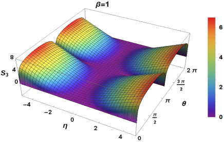
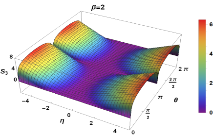
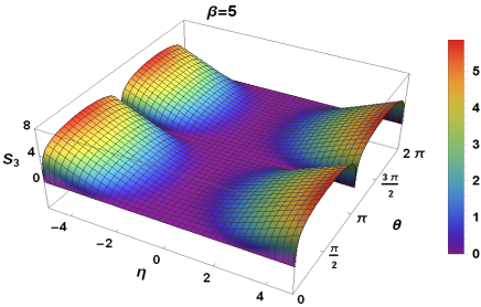
Figure 1: Rényi entropy $S_{3}$ versus the coupling parameter $\eta$ and the mixing angle $\theta$ for fixed values of the temperature $\beta=1,2,5,10$.

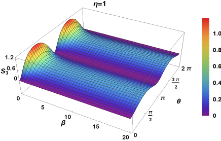
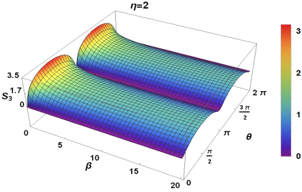
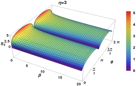
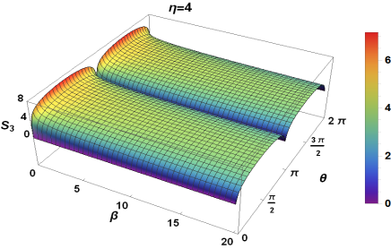
Figure 2: Rényi entropy $S_{3}$ versus the temperature $\beta$ and the mixing angle $\theta$ for fixed values of the coupling parameter $\eta=1,2,3,4$.

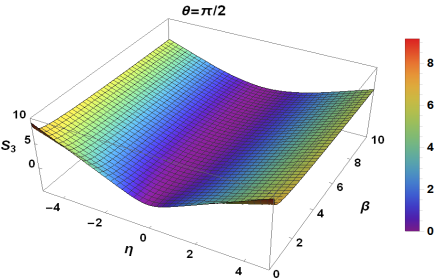
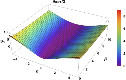
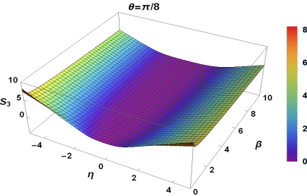
Figure 3: Rényi entropy $S_{3}$ versus the coupling parameter $\eta$ and the temperature $\beta$ for fixed values of the mixing angle $\theta=\frac{\pi}{2},\frac{\pi}{3},\frac{\pi}{4},\frac{\pi}{8}$.

Figure 2 shows the Rényi entropy $S_{3}$ as function of the temperature $\beta$ and the mixing angle $\theta$ for four values of the coupling parameter $\eta=1,2,3,4$. We observe that there are periodicity with respect to $\theta$ such that the same behavior repeats in $[0,\pi]$ and $[\pi,2\pi]$. It is clearly seen that $S_{3}$ is maximal at high temperature while it is minimal for low temperature. As long as $\eta$ is increased, we notice that $S_{3}$ increases rapidly to reach the maxima values as shown for the case $\eta=4$. In Figure 3, we present the Rényi entropy $S_{3}$ as function of the coupling parameter $\eta$ and the temperature $\beta$ for fixed values of the mixing angle $\theta=\frac{\pi}{2},\frac{\pi}{3},\frac{\pi}{4},\frac{\pi}{8}$. We observe that $S_{3}$ shows a symmetric behavior with respect to the value $\eta=0$ and decreases as long as $\theta$ decreased from $\frac{\pi}{2}$ to $\frac{\pi}{8}$. We conclude that the Rényi entropy can be controlled and adjusted by different parameters to extract some information about our system. This is clearly seen from different configurations chosen to obtain such plots in many shapes of Figures 1,2,3.

4 von Neumann entropy

To accomplish our study about some entropies, we establish a relation between the von Neumann entropy and the purity function (30) of our system. This can be worked out to end up with the expression

$$S_{1}=S_{vN}\left(\eta,\theta;\beta\right)=-\ln\left(\frac{2P}{1+P}\right)-\frac{1-P}{2P}\ln\frac{1-P}{1+P}$$ (42)

which corresponds to the case $q=1$ in general form of the Rényi entropy as seen before. We notice that, such entropy is also a function of three physical parameters $\eta,\theta$ and $\beta$ characterizing our system.

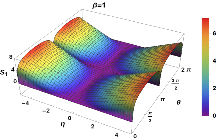
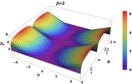
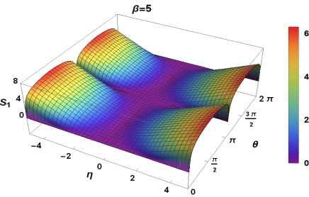
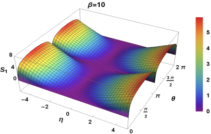
Figure 4: von Neumann entropy versus the coupling parameter $\eta$ and the mixing angle $\theta$ for fixed values of the temperature $\beta=1,2,5,10$.

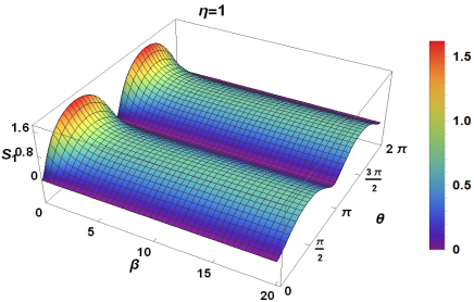
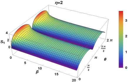
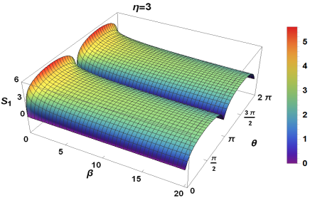
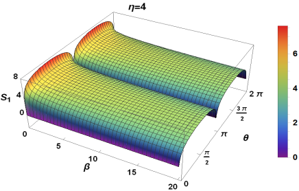
Figure 5: von Neumann entropy versus the temperature $\beta$ and the mixing angle $\theta$ for fixed values of the coupling parameter $\eta=1,2,3,4$.

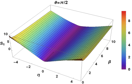
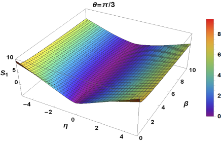
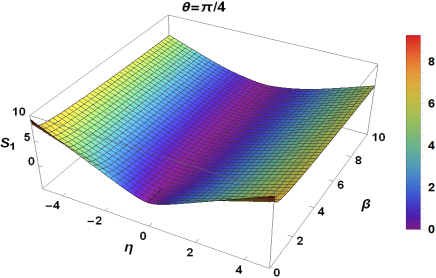
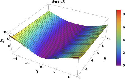
Figure 6: von Neumann entropy versus the coupling parameter $\eta$ and the temperature $\beta$ for fixed values of the mixing angle $\theta=\frac{\pi}{2},\frac{\pi}{3},\frac{\pi}{4},\frac{\pi}{8}$.

Figure 4 shows the von Neumann entropy $S_{1}$ as function of the coupling parameter $\eta$ and the mixing angle $\theta$ for fixed values of the temperature $\beta=1,2,5,10$. Figure 5 presents $S_{1}$ as function of the temperature $\beta$ and the mixing angle $\theta$ for fixed values of the coupling parameter $\eta=1,2,3,4$. Figure 6 shows $S_{1}$ as function of the the coupling parameter $\eta$ and the temperature $\beta$ for fixed values of the mixing angle $\theta=\frac{\pi}{2},\frac{\pi}{3},\frac{\pi}{4},\frac{\pi}{8}$. Compared to those of the Rényi entropy $S_{3}$, such Figures present some some similarities and differences.

To close our study it is interesting to summarize in three different tables below the most interesting form can be taken by the von Neumann entropy $S_{1}$ for particular values of the coupling parameter and mixing angle as well as low and high temperature regimes. Indeed, we start by analyzing two situations with respect to the strength of the coupling parameter $\eta$, which will allow us to underline the behavior of our system. We start with the weak coupling that is characterized by taking the limit $C_{3}\longrightarrow 0$ where the angle $\theta\longrightarrow\theta_{w}$ and the coupling $\eta\longrightarrow\eta_{w}$. In this case, (2) and (13) reduce to the following quantities

$$\theta_{w}=0,\qquad e^{2\eta_{w}}=\frac{1}{\mu^{2}}\sqrt{\frac{C_{1}}{C_{2}}}.$$ (43)

Now we consider the strong coupling limit and derive in the beginning the corresponding physical parameters. In doing so, we notice that if the limit $C_{3}\longrightarrow 2\sqrt{C_{1}C_{2}}$ is required then one can end up with the limits

$$\tan\theta_{s}\longrightarrow\frac{2\sqrt{C_{1}C_{2}}}{\mu^{2}C_{2}-\frac{C_{1}}{\mu^{2}}}\longrightarrow 0$$ (44)

$$\eta\longrightarrow\eta_{s}=+\infty,\qquad k\longrightarrow 0^{+}$$ (45)

giving rise to the results

$$ke^{2\eta_{s}}\longrightarrow\frac{C_{1}}{\mu^{2}}+\mu^{2}C_{2},\qquad\theta_{s}=\tan^{-1}\left(\frac{2\sqrt{C_{1}C_{2}}}{\mu^{2}C_{2}-\frac{C_{1}}{\mu^{2}}}\right).$$ (46)

Combining all to write the von Neumann entropies describing both limiting cases in Table 1, which is either zero or infinity.

Coupling	Angle	Purity	von Neumann entropy
$\eta$	$\theta$	$P\left(\beta\right)$	$S_{vN}\left(\beta\right)$
$\eta_{w}$	$\theta_{w}$	$1$	$0$
$\eta_{s}$	$\theta_{s}$	$0$	$\infty$

Table 1: The von Neumann entropy $S_{1}$ as function of temperature $\beta$ for strong $\eta=\eta_{s}$ and weak $\eta=\eta_{w}$ coupling.

The last situation is related to the nature of our system, which is equivalent to require that both of harmonic oscillators have the same mass $m_{1}=m_{2}$ and frequency $C_{1}=C_{2}$. Thus from (2) and (13), we end up with the constraint $\theta\longrightarrow\frac{\pi}{2}$ and $\eta\longrightarrow\eta_{id}$ with

$$e^{2\eta_{id}}=\sqrt{\frac{C_{1}+\frac{C_{3}}{2}}{C_{1}-\frac{C_{3}}{2}}}.$$ (47)

The corresponding entropies can be summarized as function of the temperature Table 2 and function of the coupling parameter $\eta_{id}$ (identical masses $m_{1}=m_{2}$) Table 3. It is clearly see that in all cases we have different forms of the von Neumann entropies, which can be simplified by replacing the purity function by their forms under the conditions taken into consideration.

Coupling	Angle	Purity	von Neumann entropy
$\eta$	$\theta$	$P\left(\beta\right)$	$S_{vN}\left(\beta\right)$
$\eta_{id}$	$\frac{\pi}{2}$	$\frac{2\sqrt{\tanh\left({\hbar}\sqrt{\frac{k_{id}}{m}}e^{\eta_{id}}\beta\right)\tanh\left({\hbar}\sqrt{\frac{k_{id}}{m}}e^{-\eta_{id}}\beta\right)}}{e^{\eta_{id}}\tanh\left({\hbar}\sqrt{\frac{k_{id}}{m}}e^{\eta_{id}}\beta\right)+e^{-\eta_{id}}\tanh\left({\hbar}\sqrt{\frac{k_{id}}{m}}e^{-\eta_{id}}\beta\right)}$	$-\ln\left(\frac{2P_{id}}{1+P_{id}}\right)-\frac{1-P_{id}}{2P_{id}}\ln\frac{1-P_{id}}{1+P_{id}}$

Table 2: The von Neumann entropy $S_{1}$ as function of temperature $\beta$ for identical particules $\eta=\eta_{id}$ and mixing angle $\theta=\frac{\pi}{2}$.

Temperature	Angle	Purity	von Neumann entropy
$\beta$	$\theta$	$P\left(\eta_{id}\right)$	$S_{vN}\left(\eta_{id}\right)$
$\infty$	$\theta_{id}=\frac{\pi}{2}$	$\frac{1}{\cosh\left(\eta_{id}\right)}$	$2\left(1-\sinh^{2}\left(\frac{\eta_{id}}{2}\right)\right)\ln\left(\cosh\left(\frac{\eta_{id}}{2}\right)\right)-\sinh^{2}\left(\frac{\eta_{id}}{2}\right)\ln\left(\sinh^{2}\left(\frac{\eta_{id}}{2}\right)\right)$
$0$	$\theta_{id}=\frac{\pi}{2}$	$\frac{1}{\cosh\left(2\eta_{id}\right)}$	$2\left(1-\sinh^{2}\left(\eta_{id}\right)\right)\ln\left(\cosh\left(\eta_{id}\right)\right)-\sinh^{2}\left(\eta_{id}\right)\ln\left(\sinh^{2}\left(\eta_{id}\right)\right)$

Table 3: The von Neumann entropy $S_{1}$ as function of coupling parameter $\eta=\eta_{id}$ with mixing angle $\theta=\frac{\pi}{2}$ for high and low temperature.

5 Conclusion

We have studied two interesting entropies for a system of two coupled harmonic oscillators by using the path integral mechanism. In doing so, we have involved a global propagator based on temperature evolution of our system. Considering a unitary transformation we were able to explicitly obtain the reduced density matrix and therefore the thermal wavefunction describing the whole spectrum of our system. These allowed us to derive the purity function characterizing the entanglement of our system in terms of temperature and coupling parameter [5].

We have used our previous results obtained in [5] to build in the first stage the Rényi entropies $S_{q}$ for all parameter $q>1$. To illustrate such study we have focused on $q=3$ and presented different plots showing the particularities of the entropy $S_{3}$. Subsequently, we have determined the von Neumann entropy $S_{1}$, which corresponds to the limiting case $q\longrightarrow 1$ of the Rényi entropies. We numerically analyzed $S_{1}$ by offering some plots under some choice of the coupling parameter, rotating angle and temperature. For its relevance we have considered particular cases and derived the corresponding von Neumann entropies. For this, we have gave three different tables showing the values can be taken by $S_{1}$ according to the nature of our system as well as the temperature regime.

References

[1]
C. E. Shannon, “A Mathematical Theory of Communication,” Bell System Technical Journal, Vol. 27, 1948, pp.
379-423 and 623-656.
[2] A. Renyi, ”On measures of entropy and information“,
Proc. Fourth Berkeley Symp. on Math. Statist. Prob., Vol. 1 (Univ. of Calif. Press, 1961), 547.
[3] H. Li and F. D. M. Haldane, Phys. Rev. Lett. 101, 010504
(2008), 0805.0332.
[4] M. Headrick, Phys. Rev. D 82, 126010 (2010), 1006.0047.
[5] A. Merdaci, A. Jellal, A. Al Sawalha and A. Bahaoui, J. Stat. Mech. (2018) 093101.
[6] A. Jellal, F. Madouri and A. Merdaci, J. Stat. Mech.
(2011) P09015.
[7] A. Jellal, E.H. El Kinani and M. Schreiber, Int. J. Mod.
Phys. A 20 (2005) 1515.
[8] I. Kosztin, B. Faber and K. Schulten,
Am. J. Phys. 64 (1996) 633.
[9] M. Rossi, M. Nava, L. Reatto and D.E. Galli,
J. Chem. Phys 131 (2009) 154108.
[10] H. Kleinert, ”Path Integrals in Quantum
Mechanics, Statistics, Polymer Physics, and Financial Markets“ (World
Scientific, Singapore 2009).
[11] A. Rènyi, ”Probability Theory“ (North
Holland, Amsterdam, 1970).
[12] M. J. Bastiaans, J. Opt. Soc. Am. 1 (1984) 711;
ibid. 3 (1986) 1243.
[13] C. Tsallis, J. Stat. Phys. 52 (1988) 479.
[14] G. Adesso, A. Serafini and F. Illuminati, Phys. Rev. A 70 (2004) 022318.
[15] J. Pipek and I. Nagy, Phys. Rev. A 79 (2009) 052501.
[16] G. Adesso, A. Serafini and F. Illuminati, Open Syst. Inf.
Dyn. 12 (2005) 189.