Method of Manufactured Solutions Code Verification of Elastostatic Solid Mechanics Problems in a Commercial Finite Element Solver

Abstract

Much progress has been made in advancing and standardizing verification, validation, and uncertainty quantification practices for computational modeling in recent decades. However, examples of rigorous code verification for solid mechanics problems in the literature remain scarce, particularly for commercial software and for the non-trivial large-deformation analyses and nonlinear materials typically needed to simulate medical devices. Here, we apply the method of manufactured solutions (MMS) to verify a commercial finite element code for elastostatic solid mechanics analyses using linear-elastic, hyperelastic (neo-Hookean), and quasi-hyperelastic (Hencky) constitutive models. Analytical source terms are generated using either Python/SymPy or Mathematica and are implemented in ABAQUS/Standard without modification to the solver source code. Source terms for the three constitutive models are found to vary nearly six orders of magnitude in the number of mathematical operations they contain. Refinement studies reveal second-order displacement convergence in response to mesh refinement for all constitutive models and first-order displacement convergence in response to increment refinement for the finite-strain problems. We also investigate the sensitivity of MMS convergence order to minor coding errors using an exploratory case. Code used to generate the MMS source terms and the input files for the simulations are provided as supplemental material.
Keywords: Code verification, verification and validation (V&V), finite element analysis (FEA), method of manufactured solutions (MMS)

1 Introduction

Computational modeling and simulation (CM&S) are anticipated to play an increasingly significant role in the medical device industry in the coming years [1]. Emerging applications of CM&S include: supporting claims of substantial equivalence or safety and effectiveness of a medical device in regulatory submissions, augmenting clinical trial data with evidence provided by “virtual clinical trials” [2, 3, 4], and providing CM&S–derived diagnostic information for clinical decision support (e.g., [5, 6]). Such uses of CM&S should be accompanied with evidence of model credibility that is commensurate with the risk associated with the intended context of use (COU) of the model [7]. Thus, as CM&S extends into higher-risk applications, there will be an increasing need for demonstrating greater CM&S credibility through rigorous verification, validation, and uncertainty quantification (VVUQ) activities.

The first step in demonstrating the credibility of a physics-based computational model is code verification, or the process of ensuring that the software solves the underlying mathematical equations correctly [8, 9, 7, 10, 11]. Rigorous methods for code verification include the method of manufactured solutions (MMS), considered the gold-standard by experts in the field [11, 10], and the method of exact solutions (MES).

The method of manufactured solutions is a mathematical approach used to verify that a given code solves the underlying governing equations correctly and that grid and time step (or pseudo-time increment) refinement reduces numerical error at the expected rate based on the underlying numerical schemes [12]. The technique was first used by Roache [13] and was later described more formally by Steinberg and Roache [14]. Oberkampf [15] also used the procedure and coined the term “method of manufactured solutions.” Although the majority of MMS applications to date have focused on verifying codes for computational fluid dynamics (CFD), application of MMS to solid mechanics software has also been performed to some extent, likely beginning with Bathe et al. [16] who used an “ad-hoc problem” with prescribed displacements to verify the order of accuracy for 2D plate finite elements. Batra and Liang [17] and Batra and Love [18] also used what they called a “method of fictitious body forces” to verify finite element codes, although only for error quantification and not for formal order of accuracy checking. Solid mechanics MMS has received more attention recently for finite deformation analyses (e.g., [19, 20]), albeit only for in-house codes where the users had direct access to solver source code.

Here, we use MMS to verify a commercial finite element code for elastostatic solid mechanics problems. We also discuss the unique considerations and challenges associated with performing MMS when the source code is not available to the user [21]. Specifically, we consider three classes of problems:

• Case I: small strain, linear elasticity

• Case II: finite strain, neo-Hookean hyperelasticity

• Case III: finite strain, Hencky elasticity [22, 23]

We follow a typical MMS workflow [12, 21] that includes the following steps:

1. choose a relevant domain for performing verification (e.g., 2D or 3D, static or time-resolved)

2. write the governing equations for the problem of interest

3. choose an analytical solution for a field of interest in the governing equations (note that the solution does not need to be physically meaningful [12, 11])

4. generate an analytical source term (i.e., a fictitious body force) to satisfy the governing equations from (2) with the analytical solution from (3)

5. implement the source term and the appropriate boundary conditions in simulation input files

6. perform grid or time/increment convergence studies and quantify the observed order of convergence ($\textrm{OOC}_{\textrm{obs}}$)

7. compare the observed ($\textrm{OOC}_{\textrm{obs}}$) and theoretical ($\textrm{OOC}_{\textrm{theor}}$) convergence rates of the underlying numerical algorithm.

Steps 1-4 are performed using a symbolic computer algebra system (Python/SymPy for Cases I and II and Mathematica for Case III). Source terms are then incorporated into ABAQUS input files (step 5) and grid and pseudo-time increment refinement studies are performed (step 6). Finally, the results from steps 6 and 7 are analyzed and plotted using Python. We have made the code used to generate the MMS source terms openly available online at https://figshare.com/s/a67927162e674bbb791e as a Python Jupyter notebook with the intent that others may use this material as a starting point for performing MMS code verification of their own solid mechanics software or applications of interest.

2 Methods

2.1 Choose the problem domain

The MMS code verification is performed in a unit cube domain (reference configuration $\mathbf{X}\in[0,1]^{3}$) with a grid spacing of $h$ (Fig. 1). All cases consider elastostatic deformation ($\frac{\partial}{\partial t}=0$).

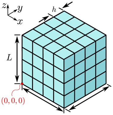
Figure 1: Unit cube domain with side lengths $L=1$ and grid spacing $h$.

2.2 Write the governing equations

The equations for conservation of linear momentum at static equilibrium, written in the current configuration $\mathbf{x}$, are

$$-\nabla_{\mathbf{x}}\cdot\boldsymbol{\sigma}\left(\mathbf{x}\right)=\mathbf{\mathbf{b}}\left(\mathbf{x}\right)$$ (1)

where $\nabla_{\mathbf{x}}\cdot$ is the spatial divergence operator, $\boldsymbol{\sigma}$ is the Cauchy stress tensor, and $\mathbf{b}$ is a body force vector with units of force per volume (both in the current configuration). To facilitate the calculation of the source term as a function of the reference configuration $\mathbf{X}$, the conservation equations are pulled back to the reference configuration using Nanson’s relation [24, 25] and written as

$$-\nabla_{\mathbf{X}}\cdot\left(J\,\boldsymbol{\sigma\left(\mathbf{X}\right)}\,\mathbf{F}^{-T}\right) =J\,\mathbf{b}\left(\mathbf{X}\right)$$ (2)

$$-\nabla_{\mathbf{X}}\cdot\mathbf{P}\left(\mathbf{X}\right) =J\,\mathbf{b}\left(\mathbf{X}\right)$$ (3)

$$-\nabla_{\mathbf{X}}\cdot\mathbf{P}\left(\mathbf{X}\right) =\boldsymbol{\phi}\left(\mathbf{X}\right)$$ (4)

where

$$\mathbf{P}\left(\mathbf{X}\right)=J\,\boldsymbol{\sigma}\left(\mathbf{X}\right)\,\mathbf{F}^{-T}$$ (5)

is the first Piola-Kirchhoff stress tensor, which maps forces in the current configuration to geometry in the reference configuration; $\mathbf{F}$ is the deformation gradient; $J$ is the determinant of $\mathbf{F}$, a measure of volume change; $\nabla_{\mathbf{X}}\cdot$ is the material divergence operator; and $\boldsymbol{\phi}\left(\mathbf{X}\right)=J\>\mathbf{b}$ is a source term with units of force (current configuration) per volume (reference configuration).

For problems using the small-strain approximation, ABAQUS uses the simplification that the Cauchy stress tensor is equal to the first Piola-Kirchhoff stress (see Reference Library > Abaqus > Theory > Elements > Continuum elements > Solid element formulation [26]). Therefore, for the small-strain case (Case I),

$$\boldsymbol{\sigma}\left(\mathbf{X}\right)\approx\mathbf{P}\left(\mathbf{X}\right)$$ (6)

and

$$-\nabla_{\mathbf{X}}\cdot\boldsymbol{\sigma}\left(\mathbf{X}\right)=\boldsymbol{\phi}\left(\mathbf{X}\right).$$ (7)

To perform MMS, we will now choose a displacement field $\mathbf{u}\left(\mathbf{X}\right)$ and solve for the source term $\boldsymbol{\phi}\left(\mathbf{X}\right)$, which is conveniently calculated based on the reference configuration alone.

2.3 Choose an analytical solution for the displacement

The displacement vector $\mathbf{u}$ describes the mapping between the current and reference configurations via the relationship $\mathbf{x}=\mathbf{X}+\mathbf{u}$. Following the MMS described by Elsworth [27], we choose the infinitely differentiable displacement field

$$\mathbf{u}=C_{1}\sin\left(n\pi X\right)\sin\left(n\pi Y\right)\sin\left(n\pi Z\right)\left(\begin{array}[]{c}1\\ 1\\ 1\end{array}\right)$$ (8)

where $C_{1}$ controls the magnitude of the displacement and $n$ controls the number of periods within the domain. Note that the displacement at the boundaries is (conveniently) zero in all directions (e.g., Fig. 2). Accordingly, a fixed zero-displacement boundary condition is enforced on the boundaries of the domain when performing simulations.

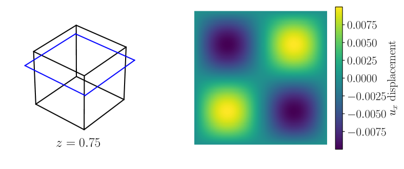
Figure 2: Contour plot showing $u_{x}$ displacement on the $z=3/4$ plane with $C_{1}=0.01$ and $n=2$.

2.4 Generate the analytical source term to satisfy the governing equations

2.4.1 Common equations

Solution of Eqn. 1 requires that the Cauchy stress is expressly written as some function of material deformation, known as the constitutive relation or model. Most constitutive models make use of the deformation gradient tensor

$$\mathbf{F} =\frac{\partial\mathbf{x}}{\partial\mathbf{X}}$$ (9)

$$=\mathbf{I}+\nabla_{\mathbf{X}}\mathbf{u}$$ (10)

where $\mathbf{I}$ is the second order identity tensor and $\nabla_{\mathbf{X}}\mathbf{u}$ is the material displacement gradient tensor. Many constitutive models also relate stress to the volume change using the quantity

$$J=\det\mathbf{F}\,.$$ (11)

Constitutive models for finite-strain problems require frame indifference so that arbitrary rotations do not produce erroneous stresses [28]. However, the deformation gradient $\mathbf{F}$ is not frame-indifferent and is not suitable for analyses involving large deformations or rotations. For these problems, a frame-indifferent tensor such as the right or left Cauchy-Green deformation tensors,

$$\mathbf{C}=\mathbf{F}^{T}\mathbf{F}$$ (12)

and

$$\mathbf{B}=\mathbf{F}\mathbf{F}^{T}$$ (13)

respectively, can be used. These tensors appropriately quantify normal and shear deformations while remaining unaffected by rigid body rotations.

2.4.2 Case I: small-strain linear elasticity

For problems with infinitesimal strains and rotations, the small-strain tensor

$$\boldsymbol{\epsilon} =\frac{1}{2}\left(\mathbf{F}+\mathbf{F}^{T}\right)-\mathbf{I}$$ (14)

$$=\frac{1}{2}\left(\nabla_{\mathbf{X}}\mathbf{u}+\nabla_{\mathbf{X}}\mathbf{u}^{T}\right)$$ (15)

is used to quantify material deformation. The constitutive model for a homogeneous linear-elastic material takes on the generalized form of Hooke’s law,

$$\boldsymbol{\sigma}=2\,\mu\,\boldsymbol{\epsilon}+\lambda\,\textrm{tr}\,\boldsymbol{\epsilon}\,\mathbf{I}\,,$$ (16)

where $\lambda$ and $\mu$ are the first and second Lamé parameters, respectively. Note that given $\lambda$ and $\mu$, the Young’s modulus $E$ and Poisson’s ratio $\nu$ required by ABAQUS can be calculated as $E=\frac{\mu\left(3\lambda+2\mu\right)}{\lambda+\mu}$ and $\nu=\frac{\lambda}{2\left(\lambda+\mu\right)}$.

2.4.3 Case II: finite-strain, neo-Hookean hyperelasticity

For the isothermal, finite-strain neo-Hookean model in ABAQUS, the strain energy density function is defined as [26]

$$W=C_{10}\left(J^{-\frac{2}{3}}\,I_{1}-3\right)+\frac{1}{D_{1}}\left(J-1\right)^{2}$$ (17)

where $C_{10}$ and $D_{1}$ are material constants and $I_{1}=\textrm{tr}\,\mathbf{B}$ is the first invariant of $\mathbf{B}$. Eqn. 17 is used to calculate the second Piola-Kirchhoff stress tensor

$$\mathbf{S}=2\frac{\partial W}{\partial\mathbf{C}}$$ (18)

which is then used to calculate the Cauchy stress via the relationship

$$\mathbf{\boldsymbol{\sigma}}=J^{-1}\mathbf{F}\mathbf{S}\mathbf{F}^{T}\,.$$ (19)

Combining Eqns. 17–18 and simplifying the expression obtains

$$\mathbf{\boldsymbol{\sigma}}=2\,C_{10}\,J^{-5/3}\left(\mathbf{B}-\frac{1}{3}\,I_{1}\,\mathbf{I}\right)+\frac{2}{D_{1}}\left(J-1\right)\mathbf{I}\,.$$ (20)

The material constants used in ABAQUS for the neo-Hookean model are related to the first and second Lamé parameters of a material linearized at the origin as follows: $C_{10}=\frac{\mu}{2}$, $K_{0}=\lambda+\frac{2\mu}{3}$, and $D_{1}=\frac{2}{K_{0}}$ [26]. Using these relationships Eqn. 20 becomes

$$\boldsymbol{\sigma}=\mu\,J^{-5/3}\left(\mathbf{B}-\frac{1}{3}\,I_{1}\,\mathbf{I}\right)+\frac{3\,\lambda+2\,\mu}{3}\left(J-1\right)\mathbf{I}$$ (21)

providing the Cauchy stress as a function of displacement-based quantites and Lamé parameters alone (i.e., $\boldsymbol{\sigma}=f\left(\mathbf{u},\,\lambda,\,\mu\right)$ since $\left\{\mathbf{B},\>J,\,I_{1}\right\}=f\left(\mathbf{u}\right)$).

2.4.4 Case III: finite-strain, Hencky elasticity

For finite-strain Hencky elasticity, the logarithmic or Hencky strain tensor

$$\boldsymbol{\epsilon}_{\ln}=\ln\,\mathbf{V}$$ (22)

is used to quantify material deformation, where

$$\mathbf{V}=\sqrt{\mathbf{B}}$$ (23)

is the left Cauchy stretch tensor. Note that here $\sqrt{\,\,}$ and $\ln$ are matrix operations (rather than element-wise operations), where $\ln$ is the principal matrix logarithm. Use of $\mathbf{V}$ in $\boldsymbol{\epsilon}_{\ln}$ makes the strain measure invariant to rigid body rotations and, thus, suitable for analyses with large deformation and rotation.

For the full 3D, finite-strain, Hencky-elastic problem, Python/SymPy alone cannot generate the source term, as SymPy fails to diagonalize the left Cauchy deformation tensor. Instead, Mathematica (v11.0, Wolfram Research, Inc., Champaign, IL) is used to directly perform the principal matrix logarithm symbolically. Because the resulting expression is already quite large at this intermediate stage (leaf count [29] $\approx$ 500,000), we also perform the remainder of the symbolic calculation for this case in Mathematica.

The constitutive model for finite-strain Hencky elasticity is the same as that for the small-strain case, with the exception that $\boldsymbol{\epsilon}$ is replaced by $\boldsymbol{\epsilon}_{\ln}$, yielding

$$\boldsymbol{\sigma}=2\,\mu\,\boldsymbol{\epsilon}_{\ln}+\lambda\,\textrm{tr}\,\boldsymbol{\epsilon}_{\ln}\,\mathbf{I}\,\textrm{,}$$ (24)

an early form of Hencky elasticity that is quasi-hyperelastic [22, 23, 30].

2.4.5 Equation summary

The constitutive model relating the Cauchy stress tensor to material deformation is defined as one of the following,

$$\boldsymbol{\sigma}=\begin{cases}\begin{aligned} &2\,\mu\,\boldsymbol{\epsilon}+\lambda\,\textrm{tr}\,\boldsymbol{\epsilon}\,\mathbf{I}&&\text{Case I}\\ &\mu\,J^{-5/3}\left(\mathbf{B}-\frac{1}{3}\,I_{1}\,\mathbf{I}\right)+\frac{3\,\lambda+2\,\mu}{3}\left(J-1\right)\mathbf{I}&&\text{Case II}\\ &2\,\mu\,\boldsymbol{\epsilon}_{\ln}+\lambda\,\textrm{tr}\,\boldsymbol{\epsilon}_{\ln}\,\mathbf{I}&&\text{Case III\,.}\end{aligned}\end{cases}$$

The first Piola-Kirchhoff stress tensor is then

$$\mathbf{P}=\begin{cases}\boldsymbol{\sigma}&\text{Case I}\\ J\,\boldsymbol{\sigma}\,\mathbf{F}^{-T}&\text{Cases II \& III}\,.\end{cases}$$ (25)

2.4.6 Source term calculation

The first Piola-Kirchhoff stress tensor $\mathbf{P}$ from Eqn. 25 is used to calculate $\boldsymbol{\phi}$, the fictitious body force (i.e., the source term) needed to satisfy the momentum equations (Eqn. 4). The source term is calculated as

$$\boldsymbol{\phi}=-\nabla_{\mathbf{X}}\cdot\mathbf{P}\left(\mathbf{X}\right)$$ (26)

where $\nabla_{\mathbf{X}}\cdot$ is the material divergence.

To calculate the source term expression, constants (Table 1) are substituted for the displacement field and the constitutive model, and the source term expression is simplified, yielding

$$\boldsymbol{\phi}=\boldsymbol{f}\left(\mathbf{X}\right)\,.$$ (27)

That is, we obtain $\boldsymbol{\phi}$ as a function of the initial reference position $\mathbf{X}$ alone. With the chosen source term constants (Table 1), two periods are contained within the unit cube domain, and peak principal strains are approximately $10\%$.

Table 1: Material and source term constants used in the MMS cases.

$C_{1}$	$n$	$\lambda$	$\mu$	$E$	$\nu$
0.01	2	100	50	$400/3$	$1/3$

2.5 Implement the source term in ABAQUS

We implement the source term in ABAQUS by prescribing loads in the reference configuration $\mathbf{X}$ using both distributed body forces (*DLOAD) and concentrated point loads (*CLOAD). The *DLOAD subroutine uses element shape functions to distribute forces over element volumes, whereas *CLOAD provides a simpler interface for prescribing discrete forces directly onto nodes of the finite element mesh. Although *DLOAD is the more obvious choice for implementing the source term, there are subtle nuances in the implementation of this subroutine in the small- and finite-strain formulation that must be accounted for. Indeed, regardless of the loading choice, correct implementation of the source term is critical for useful MMS code verification.

*DLOAD: Note that the source term $\boldsymbol{\phi}$ has units of force (current configuration) per volume (reference configuration). *DLOAD uses compatible units of force per volume, but the volume is that of the reference configuration when NLGEOM=OFF and that of the current configuration when NLGEOM=ON. Therefore, when NLGEOM=ON, we must divide $\boldsymbol{\phi}$ by $J$ (see Eqns. 1–4), i.e.

$$\textrm{DLOAD}=\begin{cases}\phi&\textrm{NLGEOM=OFF}\\ \phi/J&\textrm{NLGEOM=ON}\end{cases}\,.$$ (28)

*CLOAD: In contrast, the units of *CLOAD are force. To spread the source term over the nodes of the mesh, we can integrate $\boldsymbol{\phi}$ over the effective volume of each node, $V_{n}$, or use the simplified discrete approximation $\boldsymbol{\phi}\,V_{n}$ evaluated at each node position in $\mathbf{X}$. For interior nodes on a uniform mesh constructed from eight-node elements, the nodal volumes in the reference configuration are conveniently equal to the element volumes, as each interior node is shared by eight elements. Thus, $V_{n}=h^{3}$, where $h$ is the grid spacing. The nodal volumes for nodes on the exterior boundaries of the domain are different, but the forces at the exterior nodes are irrelevant due to the fixed zero-displacement boundary condition imposed on the outer boundaries. Therefore, the appropriate point-load forces for implementing the source term $\boldsymbol{\phi}$ are

$$\textrm{CLOAD}=\phi\,h^{3}\,.$$ (29)

This simplistic discretization of the source term introduces somewhat large numerical errors for the coarse starting meshes, but these errors are reduced with mesh refinement such that error norms still converge at a rate consistent with the underlying numerical method.

For Cases I and II, the source term is implemented in ABAQUS input files using the analytical field option in ABAQUS/CAE, which accepts symbolic Python expressions directly. However, the symbolic source term for Case III is extremely large (final leaf count in excess of $10^{7}$), making the use of CAE impractical. Thus for Case III the symbolic expression from Mathematica is exported into a Python-compatible format (Fortran syntax) and subsequently converted to C code using the SymPy autowrap module (unfuncify). ABAQUS input lines for either *CLOAD or *DLOAD are then generated and written directly from Python.

2.6 Perform grid convergence study and calculate observed order of convergence

For a given numerical method, the total numerical error $\mathcal{E}_{\text{total}}$ is the sum of discretization errors $\mathcal{E}_{\text{disc}}$, iterative convergence error $\mathcal{E}_{\text{iter}}$, and round-off error $\mathcal{E}_{\text{round-off}}$,

$$\mathcal{E}_{\text{total}}=\mathcal{E}_{\text{spatial disc}}+\mathcal{E}_{\text{temporal disc}}+\mathcal{E}_{\text{iter}}+\mathcal{E}_{\text{round-off}}\,\textrm{.}$$ (30)

Although simulations performed herein use the static form of the governing equations, nonlinear finite-strain (NLGEOM=ON) analyses in ABAQUS use a pseudo-time $t\in[0,\,1]$ over which the prescribed boundary conditions are ramped. That is, ABAQUS does not solve for the final equilibrium state directly but instead uses an updated Lagrangian approach and solves the governing equations incrementally, performing Newton–Raphson iterations to obtain a converged solution at each pseudo-time $t$. Because this incremental approach generates some numerical error, we expect the increment size to influence the accuracy of the results for the finite-strain cases (Cases II and III).

In a typical MMS analysis used to evaluate the spatial order of accuracy, the code is verified by observing the order of convergence of the total numerical error as the mesh is refined. This assumes that error sources other than spatial discretization are negligible so that

$$\mathcal{E}_{\text{total}}\approx\mathcal{E}_{\text{spatial disc}}\,\textrm{.}$$ (31)

For Eqn. 31 to hold, we must first confirm that the simulations are relatively insensitive to increment size (pseudo-time discretization), solver convergence tolerances, and round-off error. To do so, we perform simulations in ABAQUS/Standard (R2016x, Dassault Systèmes, Providence, RI) using C3D8I elements and a grid spacing of $h=0.25$, standard solver tolerances, and a fixed increment size. Solver tolerances and increment size are then each independently reduced by an order of magnitude to investigate their influences on the solution. We found that decreasing solver tolerances yields an undetectable reduction in error norms while refining the increment size from $dt=0.1$ to $dt=0.01$ yields error norm reduction on the order of $0.1\%$. However, because the error norms are smaller for the *DLOAD cases, we found that the smaller time increment size of $dt=0.01$ is required to maintain $\mathcal{E}_{\text{temporal disc}}\ll\mathcal{E}_{\text{spatial disc}}$ at the finest mesh level. In short, results from these preliminary simulations confirm that Eqn. 31 holds using the selected values and that the total numerical error is approximately equal to the spatial discretization error.

Grid refinement studies are then performed as shown in Table 2 for the three elastostatic cases using three common element types (C3D8, C3D8R, and C3D8I) and two approaches to implementing the source term (*DLOAD and *CLOAD). Again, all grid refinement simulations are performed with standard solver tolerances and a fixed increment size of $dt=0.1$ (*CLOAD) or $dt=0.01$ (*DLOAD). Uniform grid refinement is performed using a total of five meshes (Fig. 3). A consistent refinement ratio of $r=2$ is used, where $r$ is the ratio of the grid spacing from a one mesh to the next finer mesh (i.e., $r=\frac{h_{\textrm{coarser}}}{h_{\textrm{finer}}}$).

Table 2: Summary of simulation settings for each case.

	Case I	Case II	Case III
constitutive model	linear elastic	neo-Hookean	Hencky elastic
solver	Standard	Standard	Standard
NLGEOM1	OFF	ON	ON
element types2	C3D8	C3D8	C3D8
	C3D8R	C3D8R	C3D8R
	C3D8I	C3D8I	C3D8I
load type2	*DLOAD	*DLOAD	*DLOAD
	*CLOAD	*CLOAD	*CLOAD
1In ABAQUS, the NLGEOM or “nonlinear geometry” flag is used to activate the finite-strain formulation.
2Three element types and two source term implementations are investigated independently.

Figure 3: Meshes used in the grid refinement study.

After performing simulations with each mesh resolution, the results are extracted and displacement error norms are calculated. The normalized Euclidean error magnitude

$$\mathcal{E}_{\text{mag}}=\frac{1}{\sqrt{3}\,C_{1}}\sqrt{\sum_{i=1}^{3}\left(u_{\text{num}_{i}}-u_{\text{MMS}_{i}}\right)^{2}}$$ (32)

is first calculated for all nodes, where $\sqrt{3}\,C_{1}$ is the maximum displacement magnitude in the prescribed displacement field (Eqn. 8); $\boldsymbol{u}_{\text{num}}$ and $\boldsymbol{u}_{\text{MMS}}$ are the numerical and analytical displacement field vectors, respectively; and $i$ is the $i^{\text{th}}$ component of the displacement vector. The spatially averaged $L_{2}$ norm and the $L_{\infty}$ norm are then calculated as

$$L_{2}=\sqrt{\frac{1}{n}\sum_{i=1}^{n}\mathcal{E}_{\text{mag}}^{2}}$$ (33)

and

$$L_{\infty}=\max\left\{\mathcal{E}_{\text{mag}}\right\}\,,$$ (34)

where $n$ is the number of nodes in the domain. Finally, the observed order of convergence ($\textrm{OOC}_{\textrm{obs}}$) of the total numerical error is calculated as

$$\textrm{OOC}_{\textrm{obs}}=\frac{\ln\left(L_{\text{c}}/L_{\text{f}}\right)}{\ln\left(r\right)}$$ (35)

for each successive grid pair using both the $L_{2}$ or the $L_{\infty}$ error norms, where $L_{c}$ is a coarser mesh and $L_{f}$ a finer mesh in a grid pair and $r$ is the refinement ratio.

We also quantify the $\textrm{OOC}_{\textrm{obs}}$ of the pseudo-time integration using a slightly different approach. To investigate and quantify the importance of increment size, a separate increment sensitivity study is performed using increment sizes of $dt=0.2$, $0.1$, $0.05$, and $0.025$. A fixed grid spacing of $h=0.25$ is used for all cases to hold the spatial discretization error constant. We then again quantify the $L_{2}$ and $L_{\infty}$ error norms, but this time calculate the rate of convergence of the error to an asymptotic but finite value since we cannot practically achieve $\mathcal{E}_{\text{spatial disc}}\ll\mathcal{E}_{\text{temporal disc}}$. The convergence rate [11] in response to increment refinement is calculated as

$$p=\frac{\ln\left(\frac{L_{\text{inc, c}}-L_{\text{inc, m}}}{L_{\textrm{inc, m}}-L_{\text{inc, f}}}\right)}{\ln\left(r_{\textrm{inc}}\right)}\,\textrm{,}$$ (36)

where $L_{\textrm{inc}}$ is the error norm for a coarse (c), medium (m), or fine (f) increment size. Note that $p$ is a function of the relative change in the total numerical error. Thus, using a fixed mesh with a constant spatial discretization error, $p$ represents the rate at which the error due to increment discretization alone is reduced to zero.

3 Results

3.1 Source terms

For Case I, small-strain linear elasticity, the source term $\boldsymbol{\phi}$ is relatively simple and can be expressed as

$$\phi_{x} =6\pi^{2}\left(2\sin{\left(2\pi X\right)}\sin{\left(2\pi Y\right)}\sin{\left(2\pi Z\right)}-\sin{\left(\pi\left(2Y+2Z\right)\right)}\cos{\left(2\pi X\right)}\right)$$ (37)

$$\phi_{y} =6\pi^{2}\left(2\sin{\left(2\pi X\right)}\sin{\left(2\pi Y\right)}\sin{\left(2\pi Z\right)}-\sin{\left(\pi\left(2X+2Z\right)\right)}\cos{\left(2\pi Y\right)}\right)$$ (38)

$$\phi_{z} =6\pi^{2}\left(2\sin{\left(2\pi X\right)}\sin{\left(2\pi Y\right)}\sin{\left(2\pi Z\right)}-\sin{\left(\pi\left(2X+2Y\right)\right)}\cos{\left(2\pi Z\right)}\right)\>.$$ (39)

However, the source term increases in complexity from Case I to Case III, with Cases II and III consisting of on the order of $10^{4}$ and $10^{7}$ operations, respectively.

Although the source term expressions differ greatly in mathematical form, visualization of the source term fields shows that local differences are relatively subtle (Fig. 4). Indeed, maximal differences between Cases I and II and between Cases I and III are only approximately 5%, and differences between Cases II and III are even less (approximately 1%; Fig. 4).

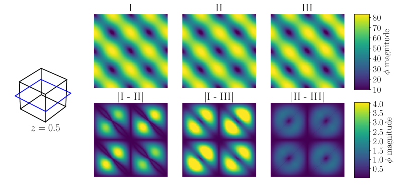
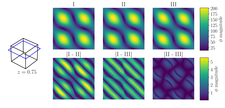
Figure 4: Contour plots of the source term magnitude on the $z=1/2$ and $z=3/4$ planes for Cases I–III. The magnitude difference between the source terms for each case are also shown.

3.2 Error norms and observed orders of convergence

Spatial convergence behavior is examined qualitatively by plotting error norms versus grid spacing on a $\log$-$\log$ scale and comparing the slopes of the resulting lines to those representing example rates of convergence (Figs. 5–6, left). For all cases investigated here, both the $L_{2}$ and $L_{\infty}$ error norms for displacement are reduced with mesh refinement at rates that approach quadratic with increasing grid refinement (Figs. 5–6, right; Tables 3–4).

Although both loading approaches yield similar convergence rates, error norms are consistently an order of magnitude lower using *DLOAD compared to *CLOAD (Fig. 5 versus Fig. 6). Convergence rates at coarse mesh resolutions are lower than theoretical using *DLOAD but higher than theoretical using *CLOAD (Table 3 versus Table 4).

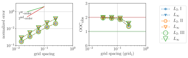
Figure 5: Normalized error norms (left) and observed orders of convergence ($\textrm{OOC}_{\textrm{obs}}$) (right) for the three cases using *DLOAD and C3D8I elements. Marker sizes are varied to allow for visualizing overlapping data points. The $\textrm{OOC}_{\textrm{obs}}$ for all cases converges towards two with decreasing grid spacing. Results for C3D8 and C3D8R element types are available online as Supplemental Material.

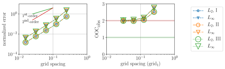
Figure 6: Normalized error norms (left) and observed orders of convergence ($\textrm{OOC}_{\textrm{obs}}$) (right) the three cases using *CLOAD and C3D8I elements. Marker sizes are varied to allow for visualizing overlapping data points. The $\textrm{OOC}_{\textrm{obs}}$ for all cases converges towards two with decreasing grid spacing. Results for C3D8 and C3D8R element types are available online as Supplemental Material.

Table 3: Theoretical and observed orders of convergence ($\textrm{OOC}_{\textrm{theor}}$ and $\textrm{OOC}_{\textrm{obs}}$) in response to grid refinement for the three MMS cases using *DLOAD and C3D8I elements. Results for C3D8 and C3D8R element types are available online as Supplemental Material.

		$\textrm{OOC}_{\textrm{obs}}$
$\textrm{grid}_{1}$ to $\textrm{grid}_{2}$	$\textrm{OOC}_{\textrm{theor}}$	$L_{2}$, I	$L_{\infty}$, I	$L_{2}$, II	$L_{\infty}$, II	$L_{2}$, III	$L_{\infty}$, III
$4^{3}$ to $8^{3}$	2	1.38	1.58	1.36	1.55	1.36	1.57
$8^{3}$ to $16^{3}$	2	1.84	1.93	1.84	1.94	1.85	1.93
$16^{3}$ to $32^{3}$	2	1.93	1.99	1.93	1.99	1.93	1.99
$32^{3}$ to $64^{3}$	2	1.96	1.99	1.97	1.99	1.96	1.98

Table 4: Theoretical and observed orders of convergence ($\textrm{OOC}_{\textrm{theor}}$ and $\textrm{OOC}_{\textrm{obs}}$) in response to grid refinement for the three MMS cases using *CLOAD and C3D8I elements. Results for C3D8 and C3D8R element types are available online as Supplemental Material.

		$\textrm{OOC}_{\textrm{obs}}$
$\textrm{grid}_{1}$ to $\textrm{grid}_{2}$	$\textrm{OOC}_{\textrm{theor}}$	$L_{2}$, I	$L_{\infty}$, I	$L_{2}$, II	$L_{\infty}$, II	$L_{2}$, III	$L_{\infty}$, III
$4^{3}$ to $8^{3}$	2	2.52	2.76	2.52	2.76	2.53	2.77
$8^{3}$ to $16^{3}$	2	2.05	2.17	2.05	2.16	2.05	2.17
$16^{3}$ to $32^{3}$	2	1.98	2.04	1.98	2.04	1.98	2.05
$32^{3}$ to $64^{3}$	2	1.98	2.01	1.98	2.01	1.99	2.02

The pseudo-time increment refinement study confirms that the increment size has no influence on the results when using the small-strain formulation (Case I) and a relatively small but quantifiable influence on the results when using the finite-strain formulation (Cases II and III). For the finite strain cases, the observed $p$-value for increment size is remarkably consistent and close to unity ($1.02\pm 0.01$), even for the coarsest increment size triplet (Table 5).

Table 5: Observed convergence rate ($p$) in response to increment refinement for the two finite-strain, updated Lagrangian MMS cases using *CLOAD and C3D8I elements.

	observed $p$
increment size triplet	$L_{2}$, II	$L_{\infty}$, II	$L_{2}$, III	$L_{\infty}$, III
0.2–0.1–0.05	1.02	1.02	1.03	1.03
0.1–0.05–0.025	1.04	1.04	1.01	1.01
0.05–0.025–0.0125	1.03	1.03	1.01	1.01
0.025–0.0125–0.00625	1.02	1.01	1.00	1.01
0.0125–0.00625–0.003125	1.01	1.01	1.00	1.00

4 Discussion and Conclusions

In this study, we perform MMS code verification of elastostatic solid mechanics problems for three distinct cases: I) small-strain linear-elasticity, II) finite-strain neo-Hookean hyperelasticity, and III) finite-strain Hencky elasticity. These cases use simple but common constitutive models that have relevance to many applications, including cardiovascular and orthopedic medical devices. In particular, most plastic and pseudoplastic or superelastic models are built upon finite-strain Hencky elasticity.

Observed orders of convergence in response to grid refinement approach quadratic for all cases (Figs. 5–6, right; Tables 3–4), agreeing closely with theory for displacement-based linear finite elements [25, 31]. The observed convergence rates in response to increment refinement for the finite-strain cases are also remarkably consistent and close to unity (Table 5), providing evidence of proper implementation of the updated Lagrangian method in ABAQUS. Collectively, these results provide evidence that coding errors do not negatively influence the simulation results for these particular classes of elastostatic problems using version R2016x of ABAQUS in our particular computing environment (a Microsoft Windows 7 workstation).

Interestingly, although the analytical source terms vary by orders of magnitude in the number of mathematical operations they contain, qualitatively the source terms are quite similar (Fig. 4). To demonstrate the sensitivity of MMS to these subtle differences, an additional exploratory case is performed pairing the constitutive model from Case III (finite-strain Hencky-elasticity) with the source terms from Case II (neo-Hookean hyperelasticity). Although the source terms for these two cases differ at most by only $\approx 1\%$ (e.g., Fig. 4), the erroneous pairing of the source term and constitutive model causes the convergence rate to fall off sharply after the grid spacing decreases below $10^{-1}$ (Fig. 7; Table 6). Accordingly, this illustrates the sensitivity of the MMS technique to subtle errors in the implementation of constitutive models, boundary conditions, body forces, or any other alteration to the underlying mathematical model, making the method a powerful tool for code testing and development.

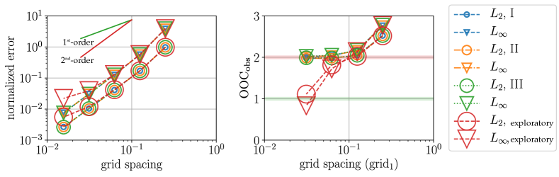
Figure 7: Normalized error norms (left) and observed orders of convergence ($\textrm{OOC}_{\textrm{obs}}$) (right) for the three cases and the exploratory case using *CLOAD and C3D8I elements. Marker sizes are varied to allow for visualizing overlapping data points. The exploratory case was performed using the finite-strain Hencky-elastic constitutive model but applying the neo-Hookean source terms. The exploratory case demonstrates the sensitivity of MMS to errors, as the maximum differences between the source terms for Cases II and III are on the order of only $1\%$.

Table 6: Theoretical and observed orders of convergence ($\textrm{OOC}_{\textrm{theor}}$ and $\textrm{OOC}_{\textrm{obs}}$) in response to grid refinement for the exploratory case (Case III constitutive model with Case II source term) using *CLOAD and C3D8I elements. Note that the $\textrm{OOC}_{\textrm{obs}}$ does not converge to the theoretical value of two despite the subtle quantitative differences between the Case II and Case III source terms.

		$\textrm{OOC}_{\textrm{obs}}$
$\textrm{grid}_{1}$ to $\textrm{grid}_{2}$	$\textrm{OOC}_{\textrm{theor}}$	$L_{2}$	$L_{\infty}$
$4^{3}$ to $8^{3}$	2	2.52	2.77
$8^{3}$ to $16^{3}$	2	2.02	2.14
$16^{3}$ to $32^{3}$	2	1.82	1.72
$32^{3}$ to $64^{3}$	2	1.11	0.83

We note that the use of commercial software poses some unique challenges for users desiring to perform code verification [21]. First, although code verification is often described as gathering evidence that the “equations are solved correctly” [11], with commercial software one must first answer the question: “what equations are being solved?” Answering this question is not always trivial. For example, initial attempts at MMS here for the simple small-strain linear-elastic problem failed (i.e., $\textrm{OOC}_{\textrm{obs}}$ tending towards zero with increasing mesh refinement) due to the use of the wrong governing equations in the generation of the analytical source term. Closer inspection of the documentation revealed that ABAQUS makes an additional approximation to the governing equations when simulating infinitesimal strain problems (Eqn. 6; [26]). After accounting for this approximation, the results were greatly improved and second-order displacement convergence rates were observed (Table 4). The neo-Hookean case was also initially challenging due to the unique form of the constitutive model used by ABAQUS [26]. Thus, determining the correct underlying governing equations for a commercial software package requires a user to at least carefully and thoroughly study the documentation. When questions arise that are not answered by the documentation alone, communication with the vendor is required to gain clarification on the precise form of the governing equations implemented in the software. Otherwise, as demonstrated here with our exploratory case, MMS code verification of the software will likely fail.

Second, the addition of an analytical source term into the governing equations is not always straightforward when using commercial software [21, 12, 11]. For example, during our initial attempts at using *DLOAD for MMS, we encountered relatively low initial error norms at the coarsest mesh level but observed convergence rates that approached zero (rather than two) with increasing mesh refinement. By running numerical experiments we discovered that the behavior of *DLOAD differs under the small- and finite-strain formulations (see Methods, Eqn. 28), and correct convergence rates were observed after accounting for this detail. For simplicity, we also used concentrated point loads (*CLOAD) weighted by their respective nodal volumes as an alternative to the built-in distributed load subroutine. In doing so, we were able to implement the analytical source term in a transparent manner. Similar strategies may also prove helpful in other situations wherein users cannot easily add a source term to the governing equations. Salari and Knupp also provide additional suggestions for implementing source terms when working with commercial software ([21], Appendix B).

Finally, although code verification activities provide valuable information to code developers, user-led code verification activities for commercial software has limited utility if problems are discovered. For instance, if a user finds an order of accuracy error in a commercial software, the user cannot investigate the source code to diagnose the problem or to make improvements—they can only submit a bug report to the software vendor in hopes that the vendor will investigate and correct the issue in a future software release. Given the limitations and difficulties associated with user-led code verification, one may argue that software vendors should bear the primary responsibility for performing rigorous code verification. Unfortunately, in practice, vendors cannot anticipate and verify every possible combination of software options that users may invoke. Many simulation packages also allow users to write their own coding extensions for custom boundary conditions or constitutive models (e.g., ABAQUS UMAT), and it would be unreasonable to expect vendors to take responsibility for verifying user-written code customizations. Indeed, code verification activities are inherently application-specific. Nevertheless, Oberkampf and Roy [10] state that although the end-user holds the ultimate responsibility for code verification, “commercial software companies are unlikely to perform rigorous code verification studies unless users request it.” Accordingly, advancing code verification practices for commercial software will likely require close collaborations between users and software developers. Releasing the documentation and source code for MMS studies as open-source software, as we do here, will allow other users to extend MMS for their applications and will facilitate the wider adoption of this powerful approach for code verification.

In conclusion, we provide rigorous code verification evidence for elastostatic analyses with three common constitutive equations using a commercial finite element solver (ABAQUS). As mentioned above, code verification exercises can only provide verification evidence for a single set of governing equations, and changing the form of a single term in the governing equations triggers the need to gather additional verification evidence [12, 11]. Hence, additional verification evidence should be generated when performing simulations with different constitutive models or when considering additional physics such as contact. With this in mind, we have provided the code used herein for generating analytical source terms as supplemental material in the form of a Python Jupyter notebook, available online at https://figshare.com/s/a67927162e674bbb791e, in the hope that it will serve as a starting template for others who desire to perform MMS code verification for their own specific applications.

Conflict of interest statement

One of the authors (NR) was formerly an employee of Dassault Systèmes Simulia, makers of ABAQUS.

References

- [1] Morrison, T. M., Pathmanathan, P., Adwan, M., and Margerrison, E., 2018. “Advancing regulatory science with computational modeling for medical devices at the FDA’s Office of Science and Engineering Laboratories”. Frontiers in Medicine, 5.
- [2] Himes, A., Haddad, T., and Bardot, D., 2016. “Augmenting a clinical study with virtual patient models: Food and Drug Administration and industry collaboration”. Journal of Medical Devices, 10(3), p. 030947.
- [3] Himes, A., 2018. “The use of computational modeling and simulation to create virtual patients: Application to cardiac pacing and defibrillation systems”. Journal of Cardiovascular Translational Research, 11(2), April, pp. 89–91.
- [4] Haddad, T., Himes, A., and Campbell, M., 2014. “Fracture prediction of cardiac lead medical devices using Bayesian networks”. Reliability Engineering & System Safety, 123, pp. 145–157.
- [5] Taylor, C. A., Fonte, T. A., and Min, J. K., 2013. “Computational fluid dynamics applied to cardiac computed tomography for noninvasive quantification of fractional flow reserve: Scientific basis”. Journal of the American College of Cardiology, 61(22), pp. 2233–2241.
- [6] Zarins, C. K., Taylor, C. A., and Min, J. K., 2013. “Computed fractional flow reserve () derived from coronary CT angiography”. Journal of Cardiovascular Translational Research, 6(5), pp. 708–714.
- [7] ASME V&V 40 – 2018. Assessing credibility of computational models through verification and validation: application to medical devices. American Society of Mechanical Engineers.
- [8] ASME V&V 10 – 2006 (R2016). Guide for verification and validation in computational solid mechanics. American Society of Mechanical Engineers.
- [9] ASME V&V 20 – 2009 (R2016). Standard for verification and validation in computational fluid dynamics and heat transfer. American Society of Mechanical Engineers.
- [10] Oberkampf, W. L., and Roy, C. J., 2010. Verification and validation in scientific computing. Cambridge University Press.
- [11] Roache, P. J., 2009. Fundamentals of verification and validation. Hermosa Albuquerque, NM.
- [12] Roache, P. J., 2002. “Code verification by the method of manufactured solutions”. Journal of Fluids Engineering, 124(1), pp. 4–10.
- [13] Roache, P. J., 1972. Computational fluid dynamics. Hermosa publishers.
- [14] Steinberg, S., and Roache, P. J., 1985. “Symbolic manipulation and computational fluid dynamics”. Journal of Computational Physics, 57(2), pp. 251–284.
- [15] Oberkampf, W., Blottner, F., and Aeschliman, D., 1995. “Methodology for computational fluid dynamics code verification/validation”. In Fluid Dynamics Conference, p. 2226.
- [16] Bathe, K.-J., Luiz Bucalem, M., and Brezzi, F., 1990. “Displacement and stress convergence of our MITC plate bending elements”. Engineering Computations, 7(4), pp. 291–302.
- [17] Batra, R., and Liang, X., 1997. “Finite dynamic deformations of smart structures”. Computational Mechanics, 20(5), pp. 427–438.
- [18] Batra, R., and Love, B., 2006. “Consideration of microstructural effects in the analysis of adiabatic shear bands in a tungsten heavy alloy”. International Journal of Plasticity, 22(10), pp. 1858–1878.
- [19] Chamberland, É., Fortin, A., and Fortin, M., 2010. “Comparison of the performance of some finite element discretizations for large deformation elasticity problems”. Computers & Structures, 88(11-12), Jun, pp. 664–673.
- [20] Kamojjala, K., Brannon, R., Sadeghirad, A., and Guilkey, J., 2015. “Verification tests in solid mechanics”. Engineering with Computers, 31(2), pp. 193–213.
- [21] Salari, K., and Knupp, P., 2000. Code verification by the method of manufactured solutions. Tech. rep., Sandia National Labs., Albuquerque, NM (US); Sandia National Labs., Livermore, CA (US).
- [22] Xiao, H., and Chen, L., 2002. “Hencky’s elasticity model and linear stress-strain relations in isotropic finite hyperelasticity”. Acta Mechanica, 157(1-4), pp. 51–60.
- [23] Xiao, H., 2005. “Hencky strain and Hencky model: extending history and ongoing tradition”. Multidiscipline Modeling in Materials and Structures, 1(1), pp. 1–52.
- [24] Truesdell, C., and Toupin, R., 1960. The Classical Field Theories. Springer Berlin Heidelberg, Berlin, Heidelberg, pp. 226–858.
- [25] Bathe, K.-J., 2006. Finite element procedures. Klaus-Jurgen Bathe.
- [26] Simulia, Dassault Systemes, 2016. “Abaqus 2016x documentation”. Providence, Rhode Island, US.
- [27] Elsworth, C. W., 2014. “Verification of an overset-grid enabled fluid-structure interaction solver”. Master’s thesis, The Pennsylvania State University.
- [28] Gurtin, M. E., 1982. An introduction to continuum mechanics, Vol. 158. Academic press.
- [29] Wolfram, 2011. “Mathematica 11 documentation”. Wolfram Research Inc., March.
- [30] Bažant, Z. P., Gattu, M., and Vorel, J., 2012. “Work conjugacy error in commercial finite-element codes: its magnitude and how to compensate for it”. Proceedings of the Royal Society-A, 468(2146), p. 3047.
- [31] Curnier, A., 2012. Computational methods in solid mechanics, Vol. 29. Springer Science & Business Media.