Unraveling the complex structure of AGN-driven outflows:
IV. Comparing AGNs with and without strong outflows

Abstract

AGN-driven outflows are considered as one of the processes driving the co-evolution of supermassive black holes with their host galaxies. We present integral field spectroscopy of six Type 2 AGNs at z $<$ 0.1, which are selected as AGNs without strong outflows based on the kinematics of [O iii] gas. Using spatially resolved data, we investigate the ionized gas kinematics and photoionization properties in comparison with AGNs with strong outflows. We find significant difference between the kinematics of ionized gas and stars for two AGNs, which indicates the presence of AGN-driven outflows. Nevertheless, the low velocity and velocity dispersion of ionized gas indicate relatively weak outflows in these AGNs. Our results highlight the importance of spatially-resolved observation in investigating gas kinematics and identifying the signatures of AGN-driven outflows. While it is unclear what determines the occurrence of outflows, we discuss the conditions and detectability of AGN-driven outflows based on a larger sample of AGNs with and without outflows, suggesting the importance of gas content in the host galaxies.

1. Introduction

Since the discovery of the correlation between masses of super-massive black holes (SMBHs) and global properties of their host galaxies (Ferrarese & Merritt 2000; Gebhardt et al. 2000), the co-evolution of galaxies and SMBHs has become an important topic in studying galaxy formation and evolution (Alexander & Hickox 2012; Kormendy & Ho 2013; Heckman & Best 2014). As AGN feedback may play a crucial role in regulating the growth of SMBHs and galaxies, various feedback mechanisms have been included in current semi-analytic models and numerical simulations to reproduce the properties of massive galaxies (e.g., Di Matteo et al. 2005; Springel et al. 2005; Croton et al. 2006; Hopkins et al. 2006), as well as the observed black hole mass correlations with host galaxy properties (Kormendy & Ho 2013).

As a potential channel of AGN feedback, outflows have been investigated in both local and distant AGN host galaxies (see Elvis 2000; Veilleux et al. 2005; Fabian 2012 and Heckman & Best 2014 for reviews). Based on different tracers of gas kinematics, a growing body of statistical works have revealed the evidence of non-gravitational motions in the narrow line regions (NLRs), indicating that gaseous outflows are prevalent among AGNs (e.g., Nesvadba et al. 2008; Wang et al. 2011; Zhang et al. 2011; Harrison et al. 2012; Mullaney et al. 2013; Bae & Woo 2014; Genzel et al. 2014; Woo et al. 2016; Wang et al. 2018; Rakshit & Woo 2018). Recent spatially resolved observations have began to map the detailed properties of AGN-driven outflows in a multi-phase view. Based on the integral-field-spectroscopy (IFS) observations of optical forbidden lines (e.g. [O iii] $\lambda$5007Å line), extensive studies have measured the geometry, kinematics, and energy of ionized gas outflows in the NLRs of local AGNs and high-z QSOs (e.g., Sharp & Bland-Hawthorn 2010; Storchi-Bergmann et al. 2010; Liu et al. 2013a, b; Rupke & Veilleux 2013; McElroy et al. 2015; Karouzos et al. 2016a, b; Bae et al. 2017; Kang & Woo 2018). With the advent of near-infrared IFS and radio interferometry observations, massive outflows of neutral and molecular gas have also been discovered and characterized in different objects and samples (e.g. Feruglio et al. 2010; Cicone et al. 2012; Maiolino et al. 2012). However, the role of AGN-driven outflows is not fully understood as the observational studies provide no strong constraint on how AGN-driven outflows quench or enhance star formation.

Using a large sample of Type 2 AGNs at low-z, Woo et al. (2016) performed a statistical study to constrain the properties and fraction of ionized gas outflows as well as their relation to AGN energetics (see also Bae & Woo 2014; Woo et al. 2017; Kang et al. 2017). They find that ionized gas outflows are ubiquitous among luminous Type 2 AGNs. In a series of studies for investigating the detailed properties of ionized gas outflows, Karouzos et al. (2016a, b), Bae et al. (2017) and Kang & Woo (2018) have carried out IFS observations of a luminosity-limited sample selected from Woo et al. (2016). They have established a set of robust methods to properly perform spatial and kinematic decomposition of the ionized gas emission, with which they effectively identify AGN-driven outflows and constrain the size, velocity, and kinetic energy of outflows (see 3.2 for details).

In this paper, we present a spatially resolved study of six Type 2 AGNs, which are identified as no/weak outflow AGNs by Woo et al. (2016), due to the lack of strong signature of outflows in the SDSS spectra. Using the Gemini/GMOS-IFU data, we investigate the differences of gas properties between AGNs with and without strong outflows. We describe the sample and observations in section 2, and data reduction and analysis in section 3. We present the main results in section 4. Discussion and summary follow in section 5 and 6.

2. Sample and observations

2.1. Sample selection

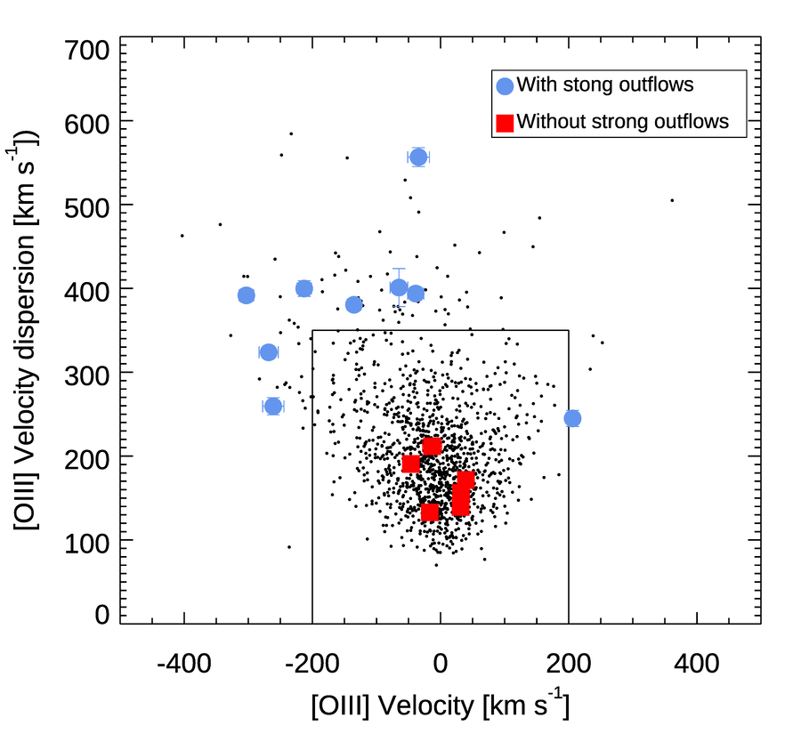
Figure 1.— [O iii] velocity versus velocity dispersion (VVD) diagram. The AGNs without strong outflows, which are selected for this study (red circles) are compared to the AGNs with strong outflows in our previous studies (blue circles). The selection criteria of strong outflows are indicated by the solid box as adopted by Karouzos et al. (2016a); Kang & Woo (2018). The luminosity-limited sample of local AGNs is denoted with black dots (Woo et al., 2016).

Table 1Properties of the sample based on the SDSS spectra and the log of observations

ID	z	V${}_{\mbox{[O\,{iii}]}}$	$\sigma_{\mbox{[O\,{iii}]}}$	$\log{\mbox{L}_{\mbox{[O\,{iii}]}}}$	$\log{\mbox{L}_{\mbox{[O\,{iii}];cor}}}$	mr	$\log{\mbox{M}_{\ast}}$	b/a	Date	texp	Seeing	AM
		[km s-1]		[erg s-1]		[AB]	M⊙			[min]	[″]
(1)	(2)	(3)	(4)	(5)	(6)	(7)	(8)	(9)	(10)	(11)	(12)	(13)
J084344+354942	0.0541	-46	191	41.7	42.7	14.70	11.07		04/12/16	40.5	0.64	1.04
J101936+193313	0.0647	-17	133	41.4	42.1	16.20	10.51	0.60	04/12/16	96	0.64	1.03
J105833+461604	0.0397	31	139	40.9	41.5	13.94	11.06	0.89	04/12/16	40.5	0.64	1.14
J115657+550821	0.0796	32	156	41.2	42.1	15.70	11.02	0.84	04/13/16	144	1.00	1.22
J131153+053138	0.0873	39	172	41.5	42.1	15.92	10.93	0.85	04/12/16	144	0.64	1.04
J161756+221943	0.1020	-13	212	40.9	41.9	15.64	11.34	0.85	04/13/16	144	1.00	1.04

Note. — Col. 1: target ID; Col. 2: redshift; Col. 3: [O iii] velocity shift with respect to the systemic velocity; Col. 4: [O iii] velocity dispersion; Col. 5: dust-uncorrected [O iii] luminosity; Col. 6: dust-corrected [O iii] luminosity (see Bae & Woo 2014); Col. 7: r-band magnitude from the SDSS photometry; Col. 8: stellar mass from SDSS (Bae & Woo, 2014; Woo et al., 2016); Col. 9: minor-to-major axis ratio; Col. 10: date of GMOS observations; Col. 11: exposure time; Col. 12: seeing; Col. 13: average airmass.

In order to compare the detailed properties of ionized gas in the AGNs with and without strong outflows, we selected AGNs with no strong signature of outflows from a large sample of $\sim$ 39,000 Type 2 AGNs at z $<$ 0.3, which was used in our previous statistical study (Woo et al. 2016) based on the archival spectra of the Sloan Digital Sky Survey. While AGNs with strong outflows were identified by tracing the extreme kinematic signatures of ionized gas manifested as large velocity shift or large velocity dispersion of [O iii]$\lambda$5007 emission line, we selected weak/no outflow AGNs using the following criteria. First, we limited the extinction-corrected [O iii] luminosity as $L_{\mathrm{\mbox{[O\,{iii}]};cor}}>10^{42}$ erg s^-1 and set a redshift cut of z $<0.1$, as applied for selecting strong outflow AGNs by Karouzos et al. (2016a). Second, we selected AGNs with small [O iii] velocity shift (i.e., $|v_{\mbox{[O\,{iii}]}}|<50$ km s^-1) with respect to the systemic velocity, and low [O iii] velocity dispersion (i.e., [O iii] velocity dispersion is consistent with stellar velocity dispersion within 20%). The systemic velocity and stellar velocity dispersion ($\sigma_{\ast}$) were measured from stellar absorption lines in the SDSS spectra (Woo et al., 2016). In addition, we also matched stellar mass and the minor-to-major (b/a) axis ratio (i.e., inclination) of our targets with those of the AGNs with strong outflows in Karouzos et al. (2016a). As a final sample we chose six Type 2 AGNs for this study.

The properties of the selected AGNs measured from the integrated SDSS spectra are presented in Table 1. In Fig. 1, we present the [O iii] velocity-velocity dispersion (VVD) diagram to contrast the gas kinematics between AGNs with and without strong outflows (for details for AGNs with strong outflows, see Karouzos et al., 2016a; Kang & Woo, 2018), along with the luminosity-limited sample of 902 AGNs (i.e., $L_{\mathrm{\mbox{[O\,{iii}]};cor}}>10^{42}$ erg s^-1) at z $<$ 0.1 selected from Woo et al. (2016).

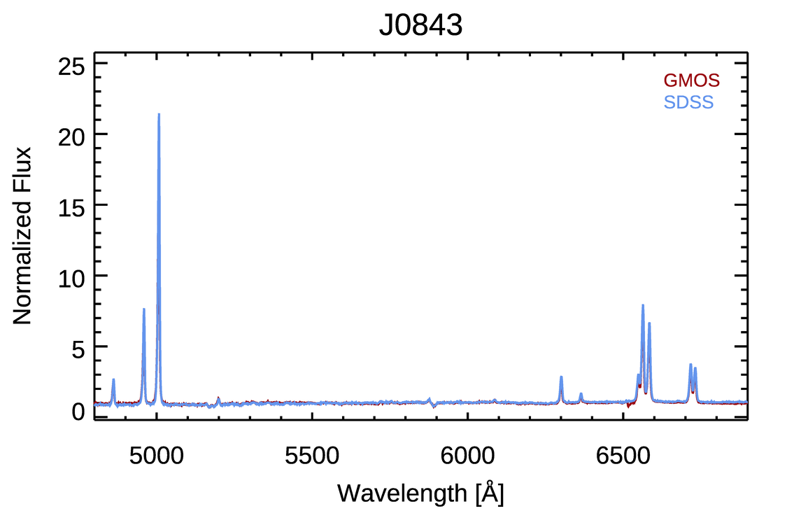
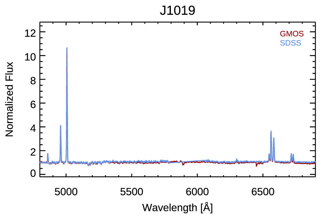
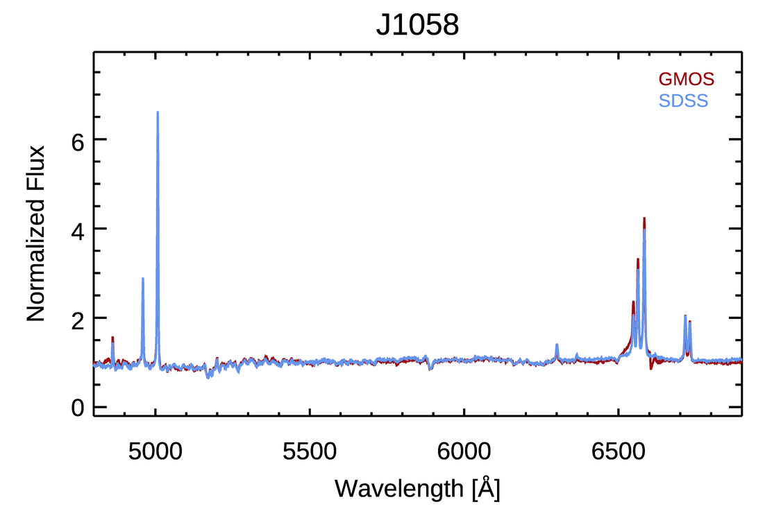
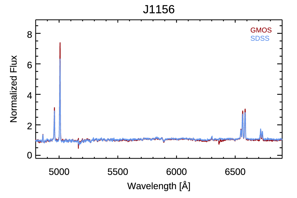
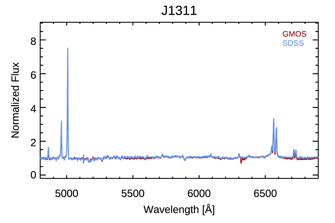
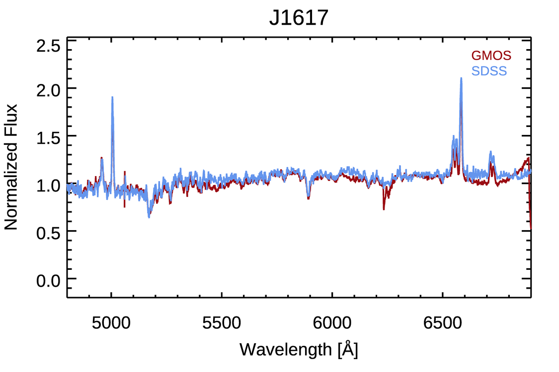
Figure 2.— Comparison of the SDSS and GMOS spectra of the sample. GMOS spectra are extracted from the central 3″spaxels. All the spectra are normalized by the median flux of their continuum.

2.2. Observations

We used the GMOS-N IFU with the 1-slit mode to observe the sample in 2016A semester (GN-2016A-Q-19, PI: Woo). The field of view ($5\farcs 0\times 3\farcs 5$) of GMOS-IFU covered 3-10 kpc scale at the redshifts of our targets, with a spaxel scale of $\sim 0\farcs 07$ ($\sim$ 60-200 pc). We used the B600 grating and a 2-pixel spectral binning, which provides a spectral resolution of R $\sim 1400$ (corresponding to a full width at half-maximum (FWHM) velocity resolution of $\sim 215$ km s^-1) over the spectral range $\sim$ 4500-6800Å. The exposure time of each target ranges from 40.5 to 144 minutes, which were determined based on the SDSS photometry. As a part of the K-GMT Science Program, our observations were performed in the priority visitor mode. All targets were observed under stable weather conditions with low wind and moderate humidity. For different targets, seeing values varied between 0$\farcs$64 and 1$\farcs$00, corresponding to sub-kpc or kpc spatial resolution (see observation details in Table 1).

3. Data reduction and analysis

3.1. Data reduction

We followed the procedure as we previously adopted (Karouzos et al. 2016a, b; Kang & Woo 2018). Here, we briefly describe the data reduction processes. We used the Gemini IRAF package to perform the standard procedures for the one-slit mode IFU. We first subtracted the CCD bias from all data frames by using the standard bias frame. Then we used the PyCosmic routine (Husemann et al. 2012) to remove cosmic rays. Based on the flat-field images from the afternoon calibration, we obtained the extraction solution of data frames. The fiber-to-fiber variation is corrected by using the twilight flat-field images. Next, we used this solution to extract spectra from the science and calibration frames. We used the arc spectra to determine the wavelength solution, which were then used to calibrate the science spectra. The sky background was corrected by using the mean sky spectra from the dedicated sky fibers. Finally, we performed flux calibration by using the spectrophotometric standard stars and built 3-D data cubes by re-sampling the spaxel size to 0$\farcs$1$\times$0$\farcs$1 (effectively oversampling the data by a factor of $\sim$ 6-10). In Fig. 2, we present the GMOS and SDSS spectra for each target. The GMOS spectra are extracted from the central 3″spaxels for this comparison.

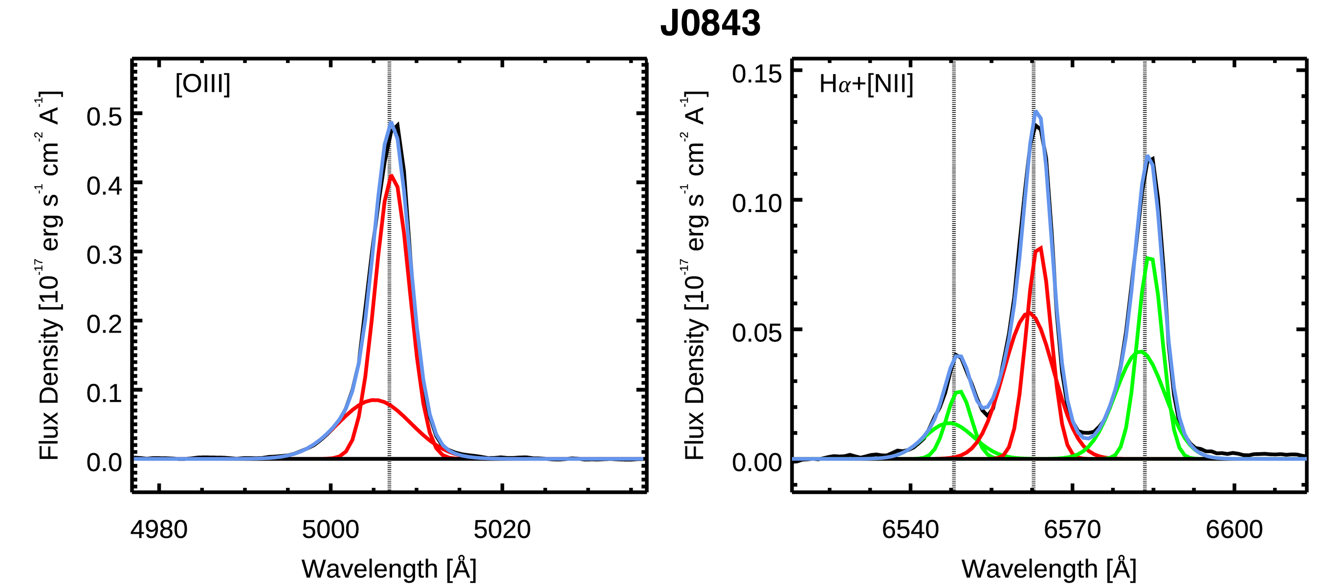
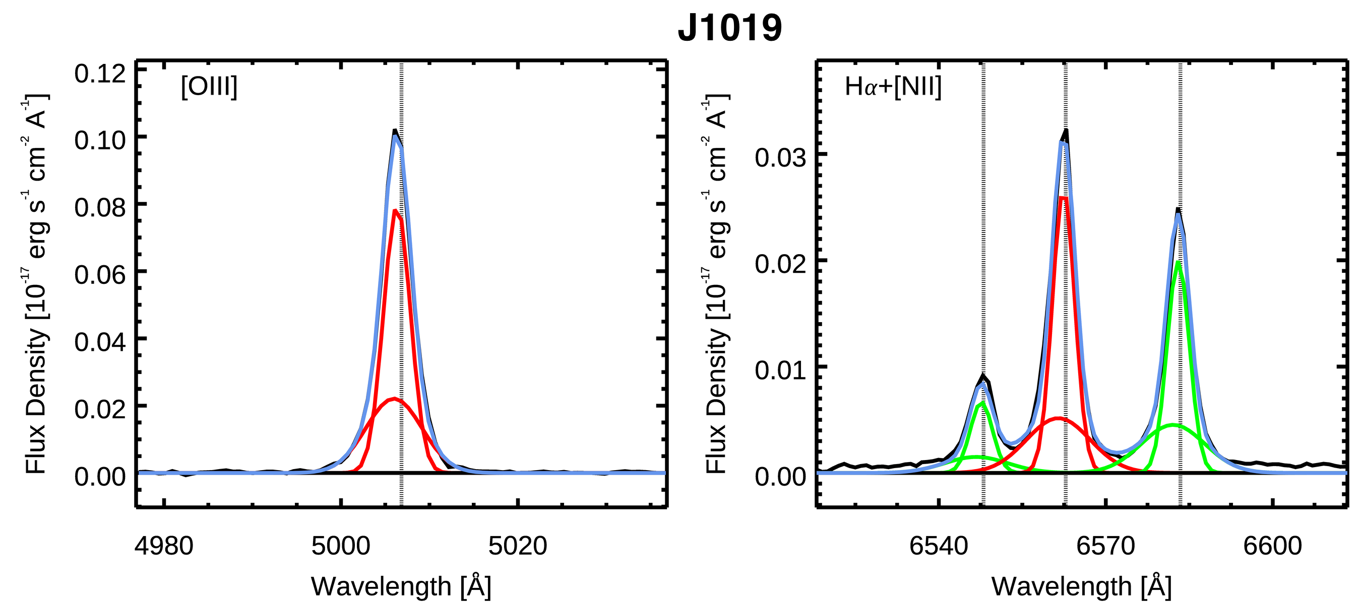
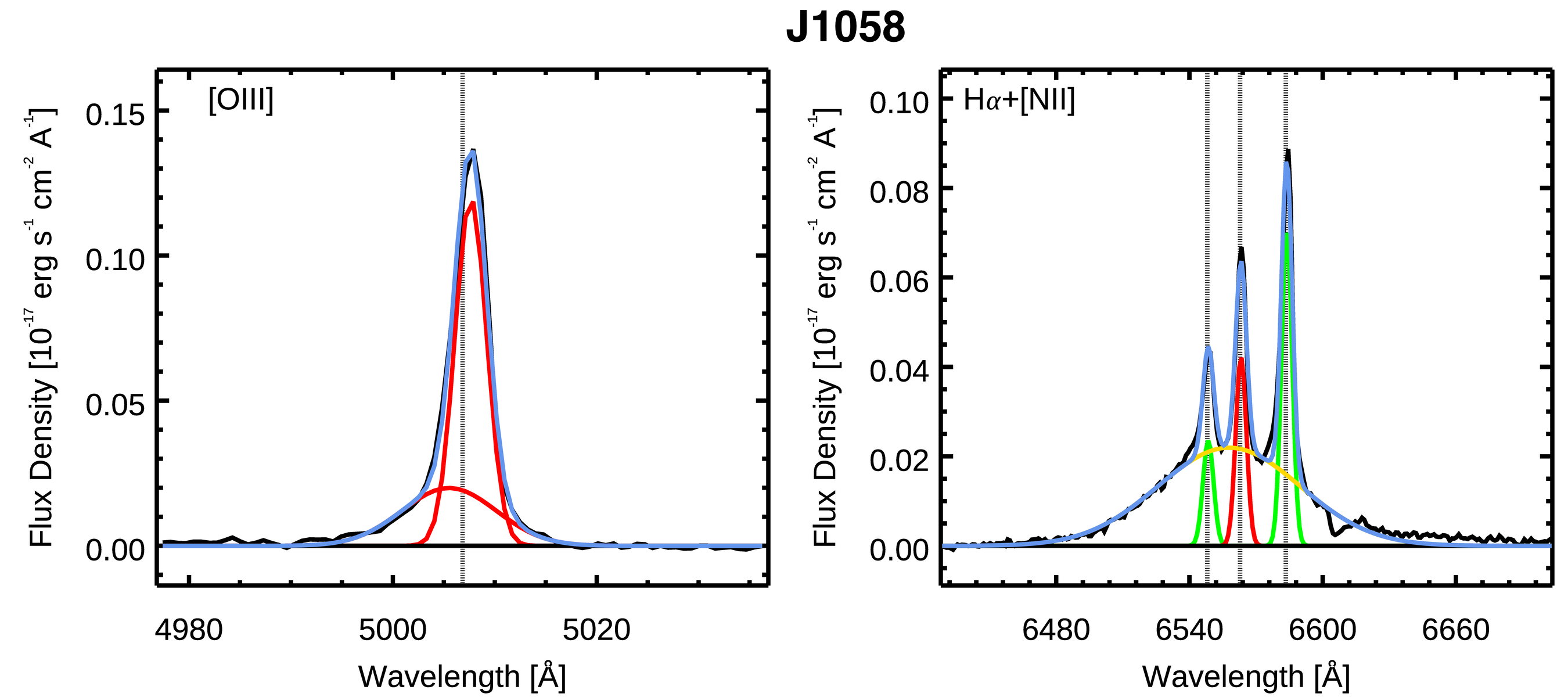
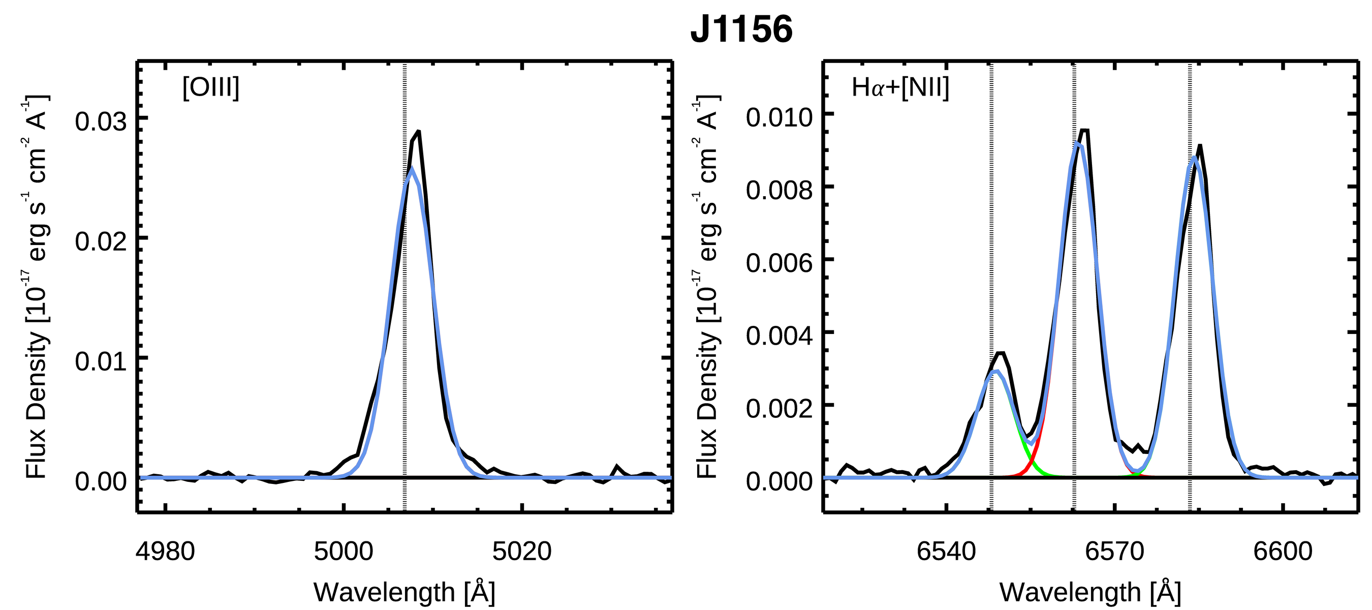
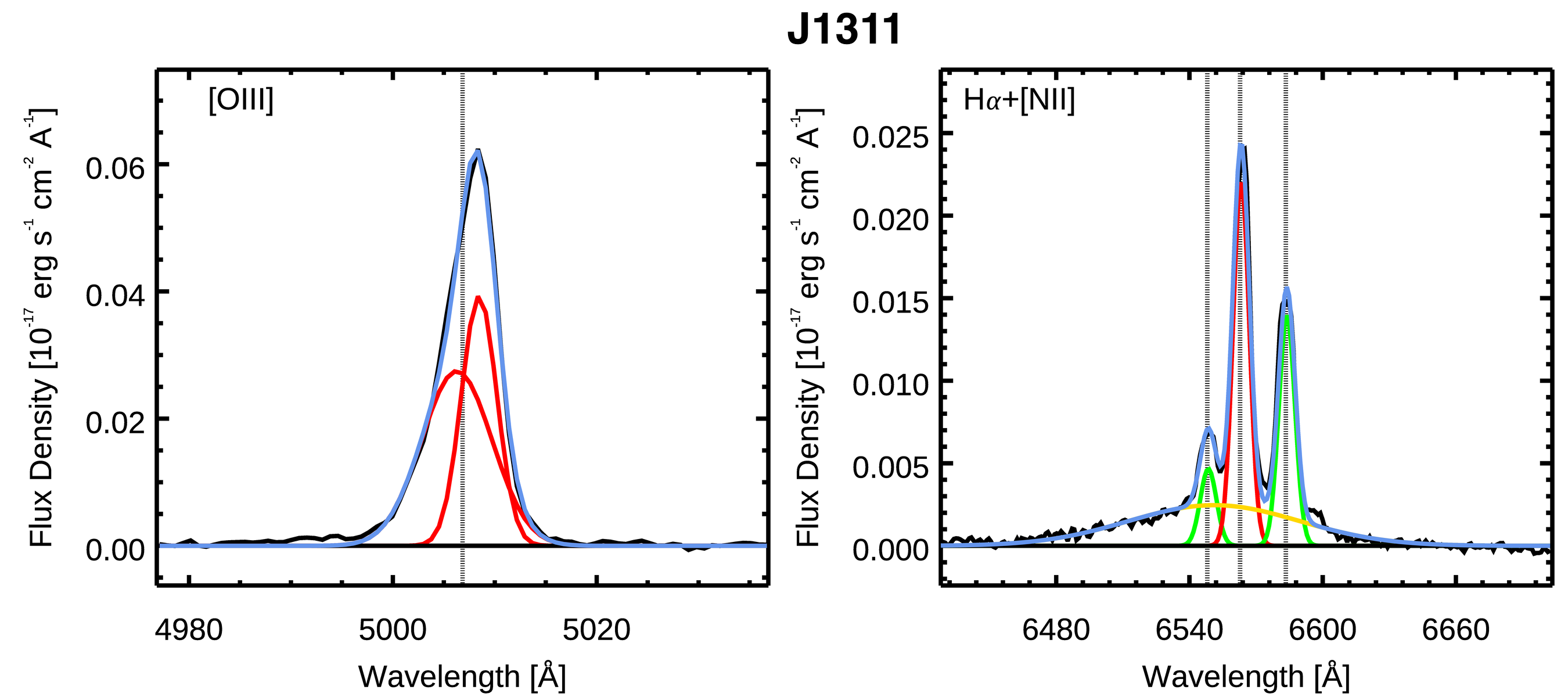
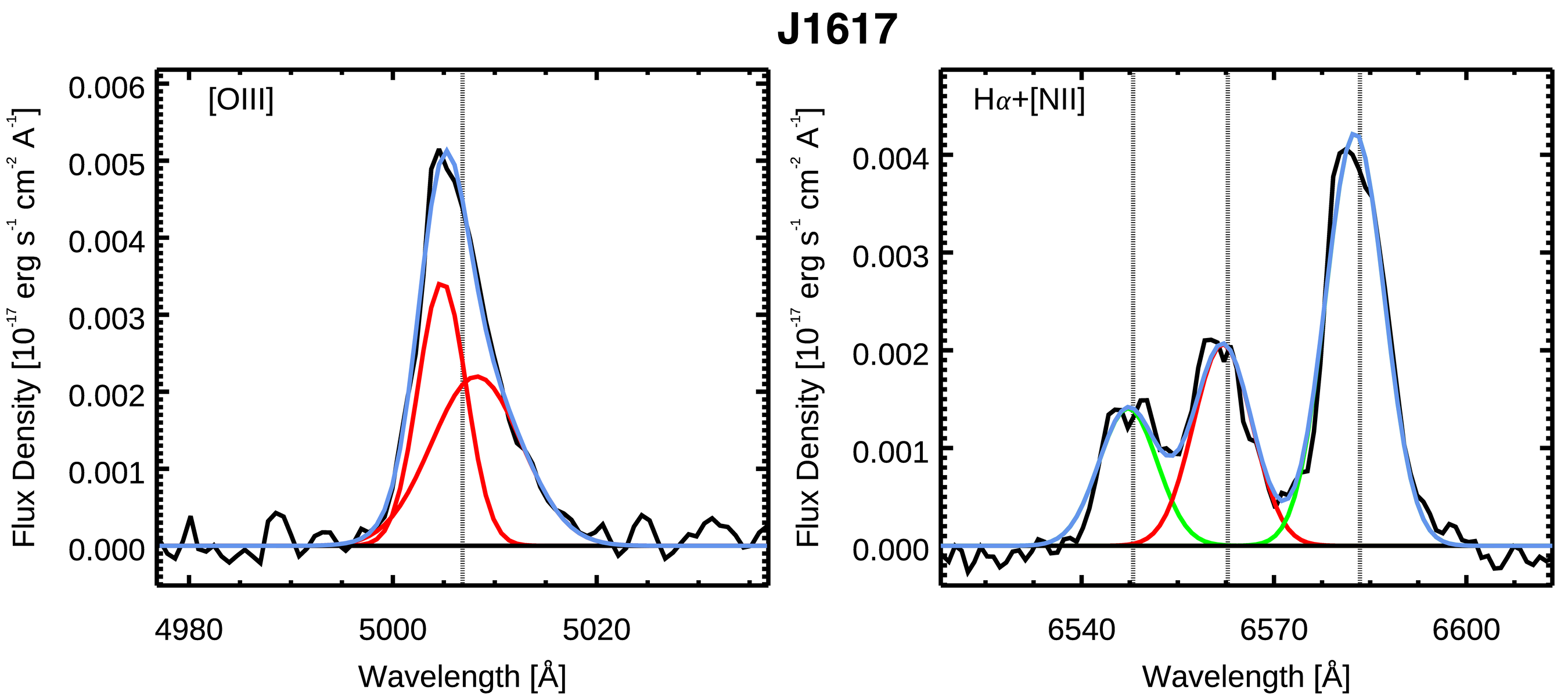
Figure 3.— Examples of emission-line fitting of [O iii] and H$\alpha$ regions in the central spaxel of each galaxy. The best fit and individual Gaussian components are shown in different colors: blue for the total profile, red for [O iii] and H$\alpha$, green for [N ii], and yellow for the very broad H$\alpha$ in J1058 and J1311. The vertical dotted lines indicate the expected center of each line based on the systemic velocity.

3.2. Data analysis

In our previous statistical and IFU-based studies of AGN-driven outflows (e.g., Bae & Woo 2014; Woo et al. 2016; Karouzos et al. 2016a, b; Woo et al. 2017; Bae et al. 2017; Kang et al. 2017; Kang & Woo 2018), we have established a set of robust methods to analyze AGN spectra and extract the kinematic properties of ionized gas. With the aim to compare the properties of ionized gas in the AGNs with and without strong outflows, we used the same analysis for our sample. Here we briefly introduce the methods as below:

First, we used the pPXF (Cappellari & Emsellem, 2004) to fit the stellar continuum and measure the stellar velocity shift (with respect to the systemic velocity) and stellar velocity dispersion for each spaxel. We modeled the continuum with 47 MILES simple-stellar population templates, which have solar metallicity, but different ages ranging from 0.63 to 12.6 Gyr (Falcón-Barroso et al., 2011). In the fitting process, the systemic velocity of each galaxy was determined from the stellar absorption lines in the spatially integrated spectra within the central 3″ spaxels.

Second, for each spaxel, we subtracted the best-fitted stellar continuum from the observed spectra to produce the pure emission-line spectrum. Then we fitted the H$\beta$, [O iii], [N ii], H$\alpha$, and [S ii] emission lines, using the Levenberg-Marquardt least-squares algorithm (Marquardt 1963; Moré 1978) as implemented in the IDL procedure MPFIT (Markwardt, 2009). We fitted each emission line with up to two Gaussian components and adopted an iterative method to determine the number of Gaussian components: (1) The peak amplitude of the broad component should be at least larger than 3 times the noise measured at the continuum near the respective emission line. (2) To avoid the detachment of two Gaussian components, the distance between their peaks should be smaller than the sum of their widths ($\sigma$). During the fitting of H$\alpha$+[N ii] and [S ii] regions, to reduce the degrees of freedom, we assume the same velocity shift (with respect to the systemic velocity) and velocity dispersion for the doublets ([N ii] and [S ii]), while the velocity dispersion is in turn tied to the velocity dispersion of individual H$\alpha$ components. In Fig. 3 we present the results of emission-line fitting for the central spaxel of each galaxy.

Third, based on the best-fitted total emission line profile (i.e., either single Gaussian model or the sum of the two Gaussian components), we calculated the first moment $\lambda_{0}$ and second moment $\Delta\lambda$ for each emission line in each spaxel, which are defined as

$$\mathrm{\lambda_{0}}=\frac{\int\lambda f_{\lambda}d\lambda}{\int f_{\lambda}d\lambda},\;\mathrm{\Delta\lambda^{2}}=\frac{\int\lambda^{2}f_{\lambda}d\lambda}{\int f_{\lambda}d\lambda}-\mathrm{\lambda_{0}}^{2}.$$ (1)

Then we calculated the line flux, the velocity shift (with respect to the systemic velocity) and the intrinsic velocity dispersion. The instrumental spectral resolution ($\sigma_{inst}\sim 91$ km s^-1) is corrected by subtracting it in quadrature from the observed velocity dispersion. For some spaxels, emission lines were not resolved and the velocity dispersion of these lines became zero after correcting for the instrumental spectral resolution. Thus, we set a value of zero for the velocity dispersion in these cases. In addition to the best-fitted total line profile, we also performed the above calculations on the profiles of each narrow and broad components for two objects, J1019 and J 1058, in which the broad component is relatively well separated from the narrow component (see Section 4.3.2). To estimate the uncertainties of the measurements, we performed Monte Carlo simulations and produced 100 mock spectra by randomizing the flux using the flux error at each wavelength. We fitted each of these spectra and adopted the standard deviation of the measurement distribution as the uncertainty. An iterative 4$\sigma$ clipping algorithm was used to exclude the bad fits in this process.

For J1058 and J1311, we find a very broad H$\alpha$ component ($\sigma\sim 1400-1700$ km s^-1) in their spectra, which could originate from the broad-line regions (BLRs). Thus, in addition to our regular double Gaussian fitting process, we fit the H$\alpha$+[N ii] region with one additional broad Gaussian component. The central wavelength and dispersion of this component was left to be free during the fitting process. The detailed description of BLRs in J1058 and J1311 will be presented in section 4.2.2. In our analysis of the other targets, we do not include this broad component because it is assumed to present the gas kinematics in the BLRs.

Based on the above analysis, we obtain the two dimensional maps of continuum flux and emission-line flux, stellar and ionized gas velocity and velocity dispersion of each target. To exclude spaxels with weak lines or bad measurements, we employ a S/N limit of 3 (based on the peak S/N) for [O iii] and H$\alpha$ emission lines. Spaxels with lower S/N are masked as gray regions in the two dimensional maps. In section 4, we will present these results.

4. Results

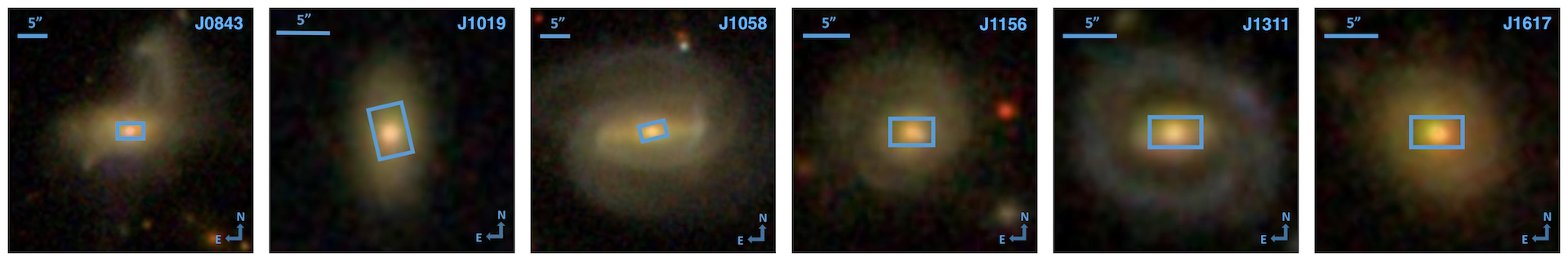
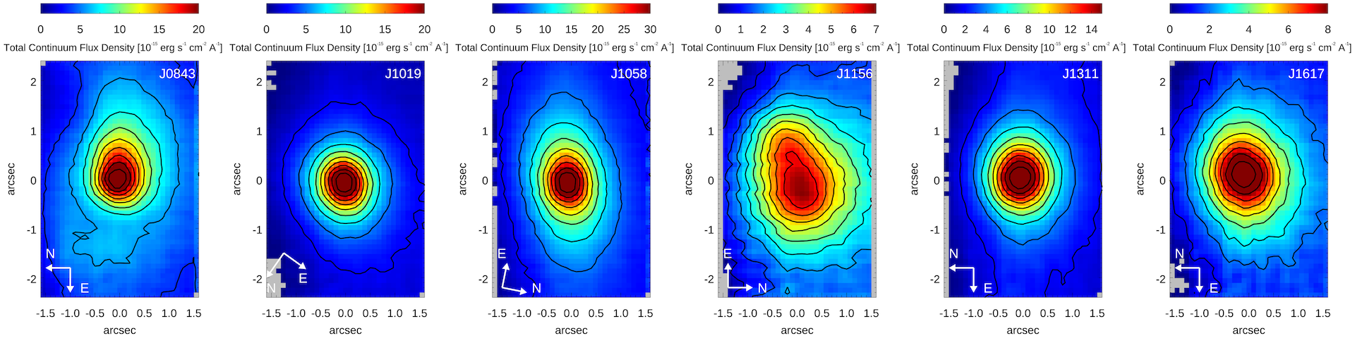
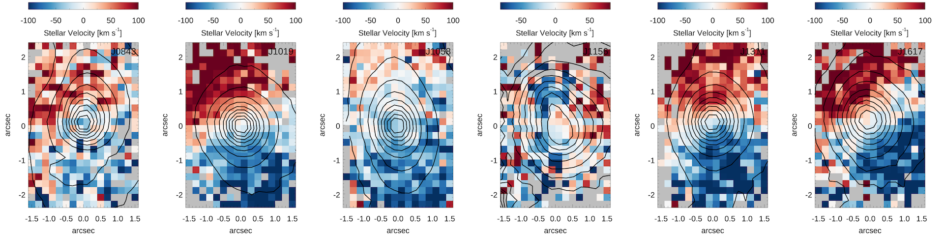
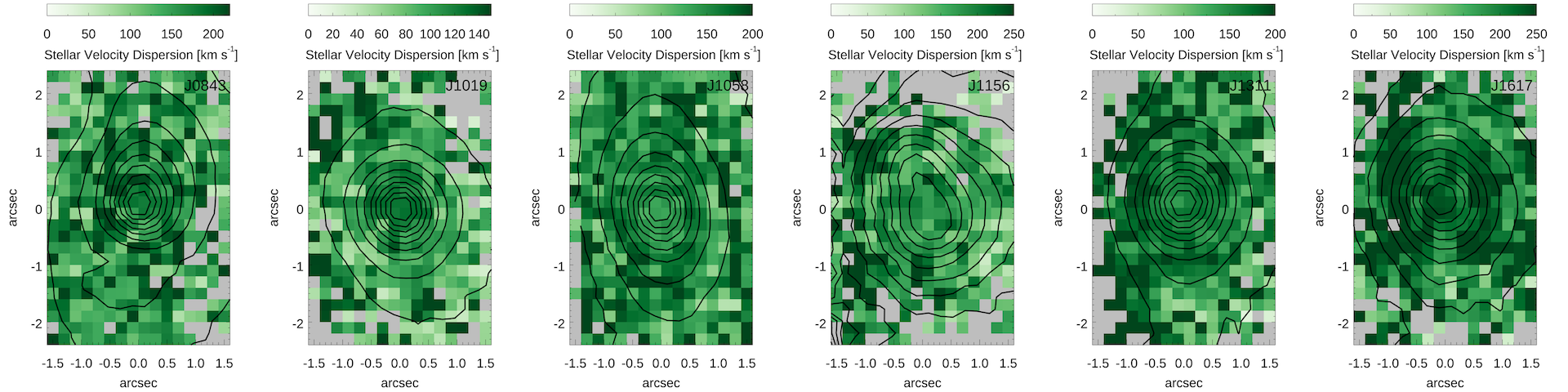
Figure 4.— Top: SDSS gri composite images. The FOV of GMOS ($5\farcs 0\times 3\farcs 5$) is shown with a blue box, while the horizontal blue bar indicates the 5$\farcs$0 scale. Second row: Continuum flux maps (integrated over the emission line-free region of the spectrum). Third row: Stellar velocity maps. Fourth row: Stellar velocity dispersion maps. The stellar velocity and velocity dispersion are obtained from the data cubes with 2 spaxels $\times$ 2 spaxels binning to increase the S/N. Gray region indicates spaxels without reliable measurements. From the second to fourth row, the black contours show the continuum flux with 10% intervals from the peak.

4.1. Host galaxy properties

In this section, we describe the properties of host galaxies of our sample. More detailed description of individual targets can be found in Appendix. In Fig. 4, we present the SDSS composite images, the continuum flux maps, as well as the stellar velocity and velocity dispersion maps. As shown in the SDSS composite images, four targets present almost face-on morphology, while J1019 appears moderately inclined (i.e., minor to major axis ratio b/a of 0.60). For J0843, the inclination is uncertain due to its disturbed morphology and tidal features, which could be caused by merging process (Lintott et al., 2011). We detect spiral arms, bars or ring structures in J1058, J1156 and J1311, which are classified as spiral galaxies in the Galaxy Zoo project (Lintott et al., 2011). We find no clear structure in J1019 and J1617. J1019 is marked as uncertain morphology in the Galaxy Zoo project, while there is no morphology classification of J1617 in the literature. The GMOS continuum flux map of each galaxy is generally consistent with the SDSS images.

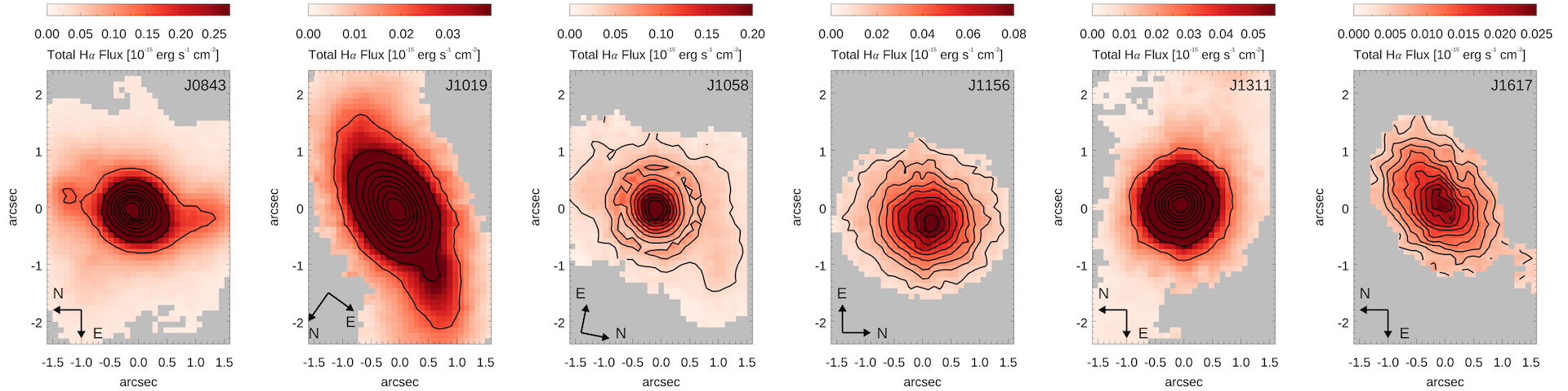
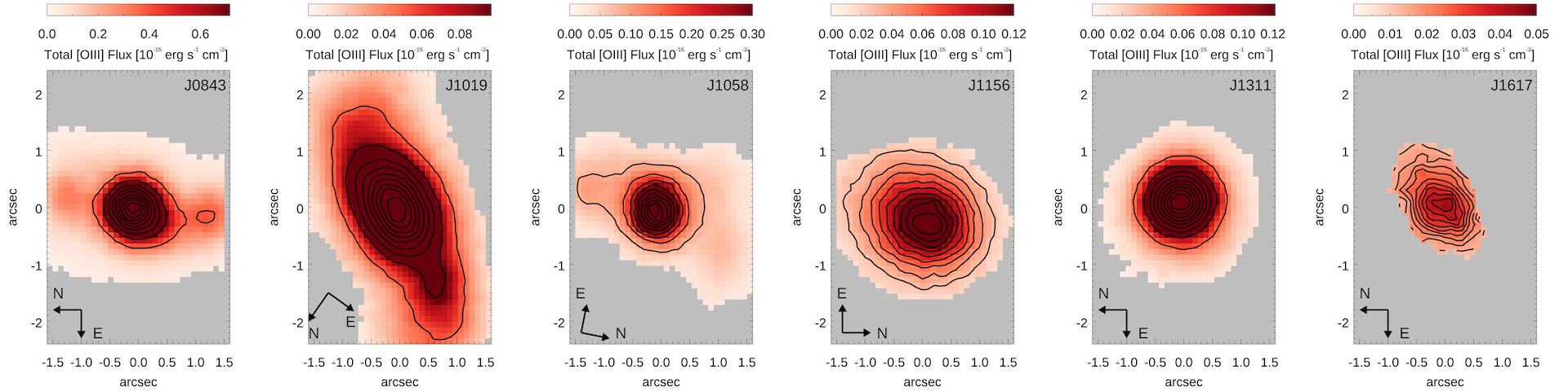
Figure 5.— H$\alpha$ (top) and [O iii] (bottom) flux maps. Black contours show the emission line flux with10% intervals from the peak. Gray spaxels indicate weak or non-detection of the emission lines (i.e., S/N $<$ 3).

For measuring stellar velocity and velocity dispersion, we used 2$\times$2 spaxel binning, in order to increase the S/N of the weak stellar lines. The spaxels with failed continuum fitting (e.g. low S/N and unreliable fitting result) are masked as gray regions. The instrumental resolution has been corrected for stellar velocity dispersion. In four targets (J1019, J1058, J1311 and J1617), the velocity maps show a butterfly shape, suggesting a clear rotation pattern, which is well aligned with the continuum flux distribution. J0843 presents a somewhat complex velocity structure, while it shows a velocity gradient along the NW-SE direction, suggesting a rotation. In J1156, the velocity map shows no clear pattern. The maximum stellar velocity ranges between 180 and 220 km s^-1 in different targets. The velocity dispersion maps show enhancements in the central parts of three galaxies (J0843, J1311, J1617), while there are no significant features in others. The typical stellar velocity dispersion ranges between 100 and 220 km s^-1.

4.2. Ionized gas flux distribution

4.2.1 H$\alpha$ and [O iii] emission

In Fig. 5, we present the maps of H$\alpha$ and [O iii] emission-line flux of our sample. H$\alpha$ and [O iii] emission lines (with S/N $>$ 3) are detected out to several kpc scales. Considering the seeing (i.e., 0$\farcs$64 and 1$\farcs$00, see Table 1), the H$\alpha$ and [O iii] emission regions are clearly resolved in all targets. Even for J1311, the spatial FWHM of [O iii] emission is $\sim 0.75$″, which is still larger than the corresponding seeing size ($0.64$″) during the observation. In three galaxies (J0843, J1058, J1617), the H$\alpha$ emission is slightly more extended than the [O iii] emission, while in J1019 and J1156, the spatial coverage of H$\alpha$ and [O iii] emission are similar. In J1311, the H$\alpha$ emission extends to the edge of the GMOS FOV, while the [O iii] emission is more concentrated in the inner region. Although the spatial coverages of H$\alpha$ and [O iii] emission regions varies among the targets, we find no significant difference in the flux distribution.

Comparing with the stellar continuum map, the H$\alpha$ and [O iii] emission is more concentrated in the inner region. In four targets (J1019, J1156, J1311, J1617), the spatial distribution of H$\alpha$ and [O iii] emission generally follows that of the stellar continuum. In contrast, J0843 and J1058 show large difference of the flux distribution between ionized gas and stars, presumably due to the complex gas kinematics in these galaxies (see Section 4.3 for details).

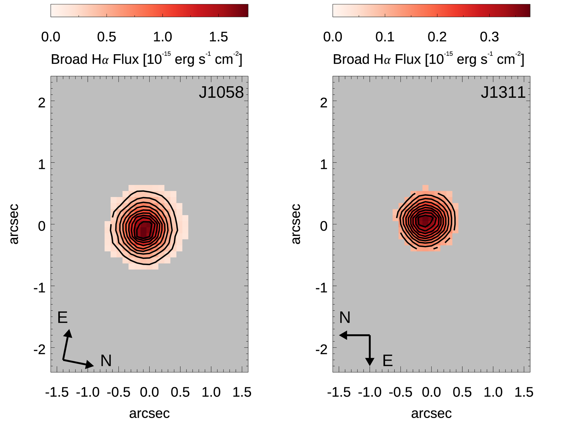
Figure 6.— Flux maps of the very broad H$\alpha$ component in J1058 and J1311. Black contours show the emission line flux with 10% intervals from the peak.

4.2.2 H$\alpha$ emission from the broad line region

As described in section 3.2, we find a very broad H$\alpha$ component in the spectra of J1058 and J1311, which is originated from the BLR. This broad component in H$\alpha$ is present within the central $\sim 1.5$″ scale (see Fig. 6). The size of the very broad H$\alpha$ emission is FWHM $\sim 0.64$″, representing the seeing size during the observation. The velocity and velocity dispersion of this component are almost constant within the detected region, confirming that the broad H$\alpha$ emission is a point source in our observation with a limited spatial resolution. The velocity shift of this component is $\sim-230$ km s^-1 and $-540$ km s^-1, while the velocity dispersion is $\sim$ 1400 km s^-1 and 1700 km s^-1, respectively, for J1058 and J1311. Using the luminosity of this H$\alpha$ component and the scaling relation calibrated by Woo et al. (2015), we estimate the black hole mass as $2.6\times 10^{6}$ $M_{\odot}$ and $4.1\times 10^{6}$ $M_{\odot}$, respectively for J1058 and J1311.

4.3. Ionized gas kinematics

4.3.1 Velocity and velocity dispersion maps

Velocity

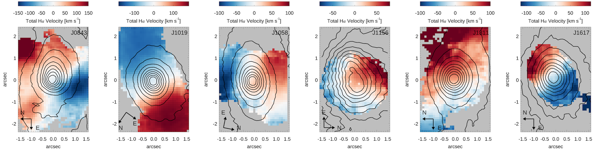
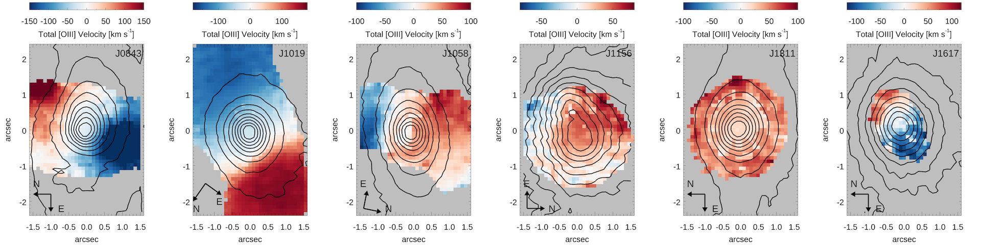
Velocity dispersion

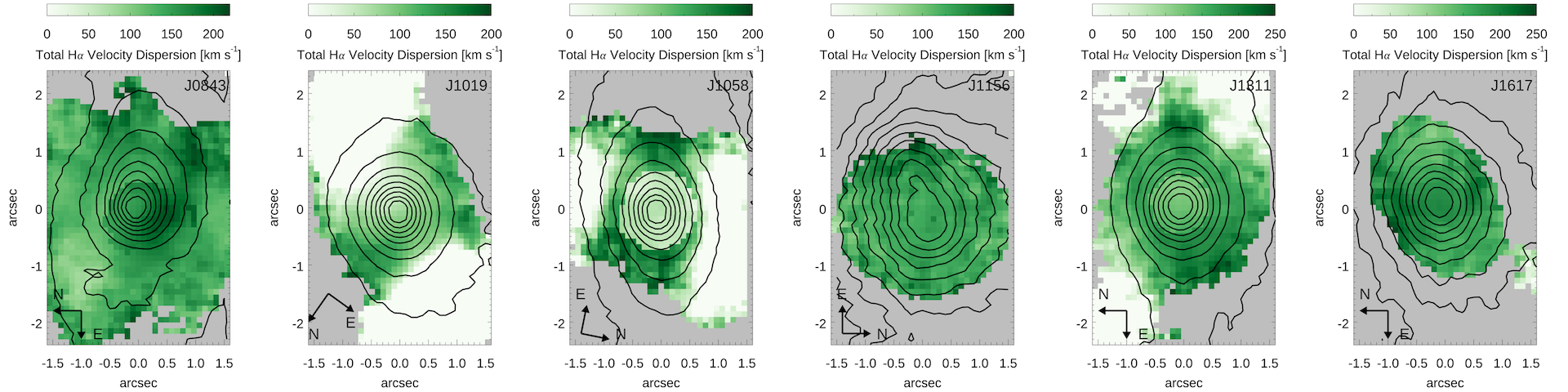
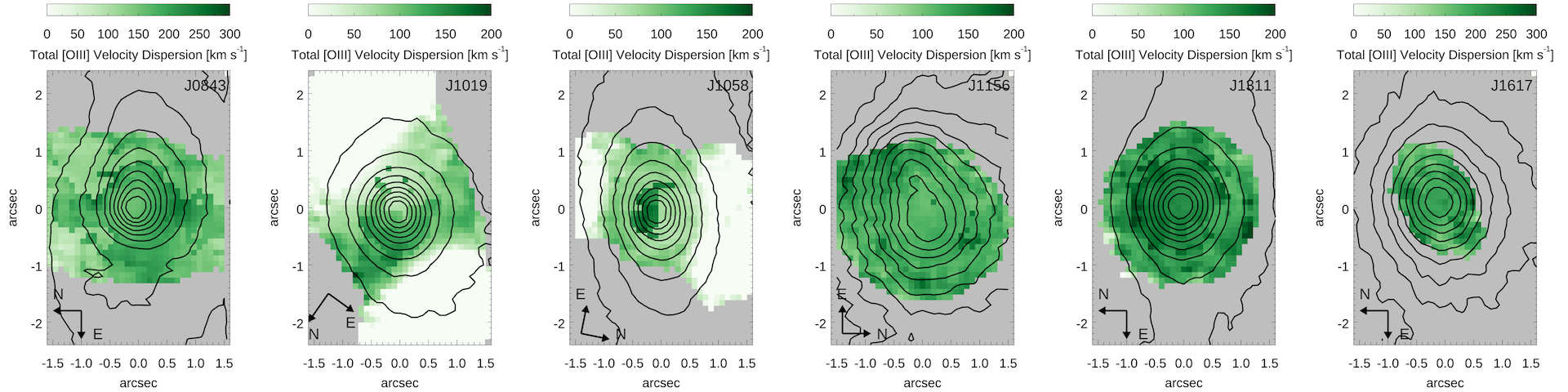
Figure 7.— Velocity and velocity dispersion maps derived from the best-fitted total profile of H$\alpha$ and [O iii] emission lines. As in Fig. 4, black contours indicate the stellar continuum flux with10% intervals from the peak. Gray spaxels indicate weak or non-detection of the emission lines (i.e., S/N $<$ 3). Note that the velocity of ionized gas is measured with respect to the systemic velocity based on stellar absorption lines at the center of each galaxy.

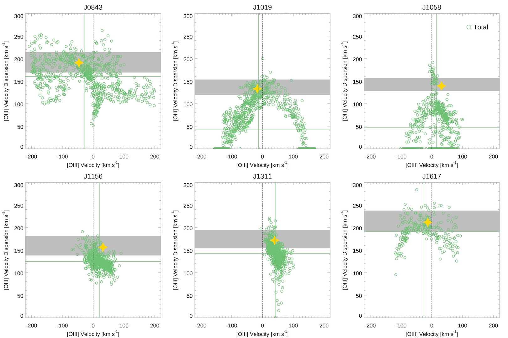
Figure 8.— VVD diagram based on the best-fitted total profile of [O iii] in each spaxel, along with the mean values (green lines). Gray-shaded stripes denote stellar velocity dispersion with a 3$\sigma$ uncertainty while gold stars indicate [O iii] velocity and velocity dispersion measured from the SDSS spectra.

In Fig. 7, we present the velocity and velocity dispersion maps derived from the best-fitted total line profile of H$\alpha$ and [O iii]. The spaxels with weak lines or bad measurements (i.e., S/N $<$ 3 for H$\alpha$ and [O iii] emission lines) are masked as gray regions in these maps. Comparing with stars, the ionized gas presents complex kinematic signatures. We describe the detailed properties of each target as below.

J0843: The kinematics of ionized gas, particularly H$\alpha$, seems affected by the merging process (see also the velocity-velocity dispersion diagram in Fig. 8), while both H$\alpha$ and [O iii] velocity maps show a rotation pattern in the NW-SE direction, which is weakly present in the stellar velocity map. While it is possible that AGN-driven outflows influence gas kinematics, but the complex nature of gas motion is probably due to the merging process.

J1019: The velocity maps of the ionized gas show an opposite spatial trend compared to the stellar velocity map. One possible explanation is that the ionized gas is counter-rotating compared to stars. The counter-rotating gas can be present due to external processes, e.g. major mergers, minor mergers or gas accretion (Corsini 2014). This phenomenon is more often detected in elliptical and lenticular galaxies, while it is relatively rare in late type galaxies (Corsini 2014; Chen et al. 2016). By examining the large scale environment using the SDSS image, we find no nearby companion galaxy, suggesting that gas supply from a nearby companion is unlikely. The bi-conical outflows driven by AGN is consistent with the observed gas kinematics, if the outflow direction is along the kinematic major axis. As predicted by the 3D bi-conical model of AGN-driven outflows (Shin et al. in prep.), the gas velocity dispersion will be enhanced in the central part of the bi-cone, due to the combined effect of gas outflows and the point spread function (PSF) smearing effect. The observed velocity dispersion of [O iii] and H$\alpha$ is consistent with this prediction. As shown in the velocity dispersion maps, the ionized gas has low velocity dispersion along the kinematic major axis, while velocity dispersion is significantly enhanced in the central region. Note that due to the limited spectral resolution, emission lines are not resolved in the outer pixels (i.e., velocity dispersion is set to 0). As the broad and narrow components of [O iii] are relatively well separated in the line profile, we also present the VVD diagram of these components in Fig. 9 (see Section 4.3.2).

J1058: [O iii] and H$\alpha$ velocity maps show that the kinematic major axis of the ionized gas is misaligned with respect to that of stars, by 40 degree. The misalignment can be caused by internal processes as well as external processes. While a mild misalignment can be caused by the effect of non-axisymmetric structures (e.g., bars, spiral arms) and decoupled stellar components, a large misalignment is mainly considered as the result of galaxy interactions or gas accretion (Dumas et al. 2007; Davies et al. 2014; Jin et al. 2016). From the large scale SDSS image, we find no nearby companion of this galaxy. Considering the clear and strong bar structure in J1058, we consider that the gravitational perturbation of large-scale bar may be responsible for producing the kinematic misalignment between gas and stars. However, as predicted by the hydrodynamical simulation of gas flows within a bar structure (Li et al., 2015), the gas velocity dispersion will be enhanced along the leading or trailing side of the bar. The observed velocity dispersion of the ionized gas contradicts to this prediction. The significant enhancement of velocity dispersion can only be observed in the central region of the galaxy, while it is very low along the kinematic major axis of the ionized gas. The bi-conical outflows driven by AGN can provide a better explanation. The outflow direction is independent of the axis of the stellar disk, and the velocity map may represent the bi-conical outflows in the N-S direction. The enhancement of velocity dispersion at the center of the bi-cone can be also naturally explained by the overlap of the approaching and receding cones due to the PSF smearing effect. Note that H$\alpha$ velocity dispersion is relatively low at the central region. However, this may be an artifact as the line profile of H$\alpha$ in the central spaxels is not very well constrained because of the presence of the very broad H$\alpha$ component (see Fig. 6).

J1156: [O iii] and H$\alpha$ velocity maps show an irregular pattern with positive velocity (i.e., redshift) in the central region, while it could be interpreted as a weak rotation. Note that stars do not show a clear rotation pattern. The velocity is limited within $\pm$100 km s^-1, while the typical velocity dispersion is $\sim$ 120 km s^-1. These kinematic properties can be interpreted as due to the face-on orientation of a rotating disk of a relatively low mass galaxy although we cannot rule out that the kinematic pattern is due to outflows.

J1311: There is clear difference between velocity maps of [O iii] and H$\alpha$. While H$\alpha$ follows the stellar rotation pattern, [O iii] shows relatively weak positive velocities (i.e., redshifts) without a clear rotation pattern. The bi-conical outflows can explain the positive velocities of [O iii], if the angle between the bi-cone axis and the dusty galactic plane is small and the approaching cone is obscured. However, [O iii] velocity is relatively small ($<$ 100 km s^-1) and [O iii] velocity dispersion is also comparable to stellar velocity dispersion. Thus, we have no strong evidence of AGN-driven outflows. The smooth distribution of [O iii] velocity dispersion may reflect the PSF smearing effect of the centrally-concentrated small scale NLR.

J1617: Both H$\alpha$ and [O iii] velocity maps show a rotation pattern, which is consistent with the stellar velocity map. The typical velocity and velocity dispersion of the ionized gas are also comparable with those of stars. We find no clear evidence of outflows.

In summary, the kinematics of the ionized gas in our sample are governed by various physical processes, including merging, AGN-driven outflow and host galaxy gravitational potential. In two targets, namely, J1019 and J1058, the ionized gas kinematics is significantly different from that of stars, which is consistent with the bi-conical outflows driven by AGN.

4.3.2 Velocity-velocity dispersion diagram

In Fig. 8, we present the velocity versus velocity dispersion (VVD) diagram of each target. As described by Karouzos et al. (2016a), the outflow components are often blueshifted and broad in the case of AGNs with strong outflows. Thus, the spaxels with outflow signatures will be located at the upper left corner of the VVD diagram. In contrast, we find no such a trend in our sample, except for J1058, for which the comparison of gaseous and stellar kinematics indicates AGN-drive outflows (S.4.3.1). In J0843, the VVD diagram shows no regulated pattern, reflecting the effect of merging on the gas kinematics. While two targets, J1156 and J1311 show neither a rotation pattern or strong outflow signatures, J1617 shows a rotation pattern without outflow signatures.

For J1019 and J1058, we also present the VVD diagram, respectively, using the narrow and broad components of [O iii] in Fig. 9, since these two objects have outflow signatures in the velocity maps. Compared to AGNs with strong outflows, the VVD diagrams of these two objects show similar patterns with the broad component extending to the upper left (i.e., high velocity dispersion and high negative velocity), which further supports the presence of AGN-driven outflows. However, the broad component of [O iii] has a mean velocity dispersion larger than stellar velocity dispersion by a factor of 1.4-1.8, indicating that [O iii] velocity dispersion is not as high as those of AGNs with strong outflows (Karouzos et al., 2016a). These results suggest that relatively weak outflows are present in J1019 and J1058.

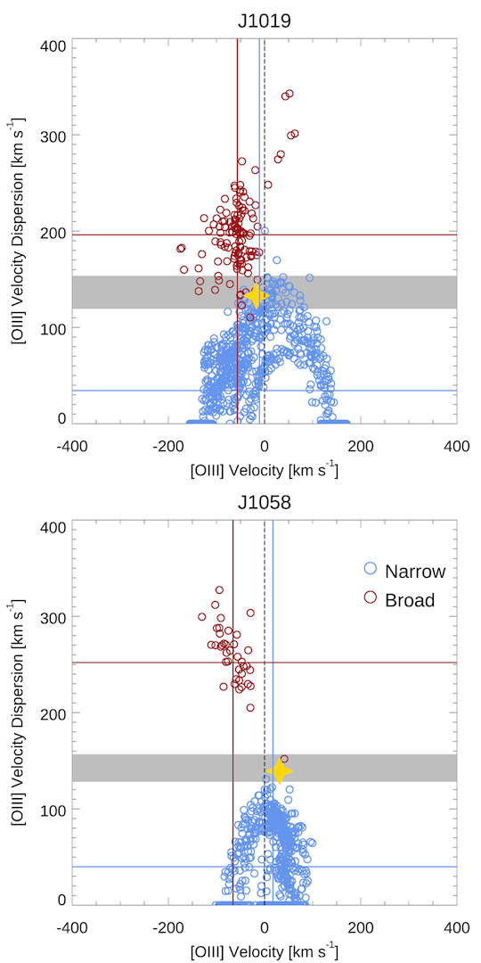
Figure 9.— VVD diagram of the broad (red) and narrow (blue) components of [O iii] for J1019 (top) and J1058 (bottom), along with the mean values (red and blue lines). Gray-shaded stripe denotes stellar velocity dispersion with a 3$\sigma$ uncertainty. Gold stars indicate[O iii] velocity and velocity dispersion measured from the SDSS spectra.

4.4. Photoionization properties

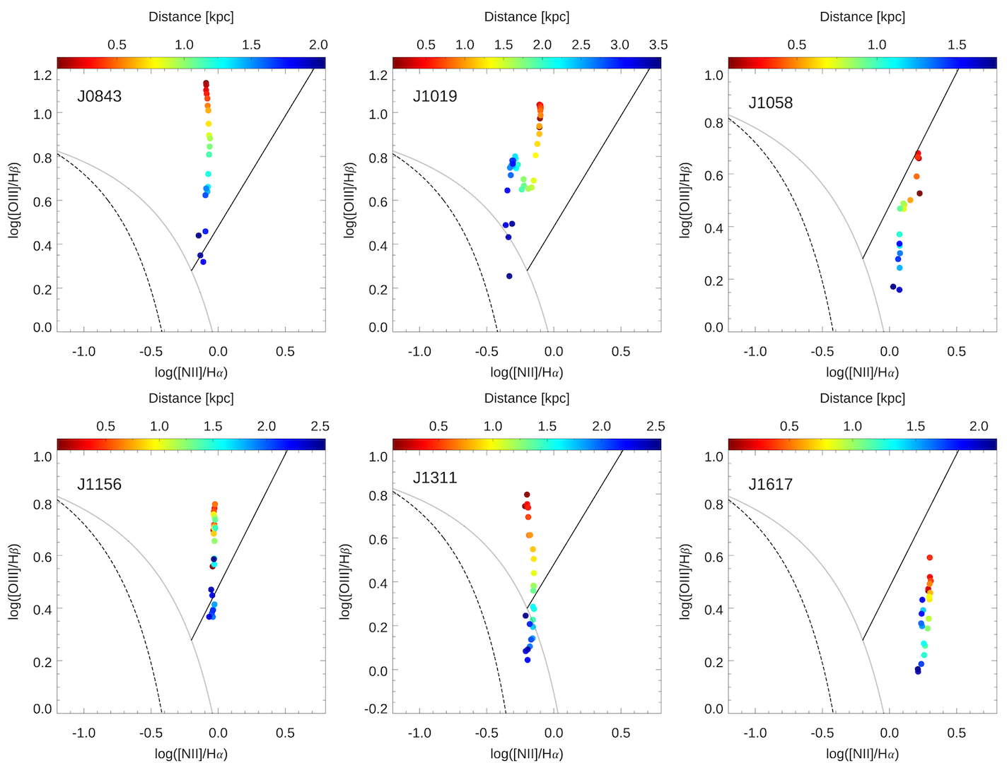
Figure 10.— Spatially resolved BPT diagrams. The mean flux ratios of [O iii]/H$\beta$ and [N ii]/H$\alpha$ are calculated within the distance bin of 0.1 kpc and color-coded accordingly. The dotted and dashed curves indicate the demarcation lines defined by Kewley et al. (2001) and Kauffmann et al. (2003), respectively. The solid line shows the Seyfert/LINER demarcation of Cid Fernandes et al. (2010).

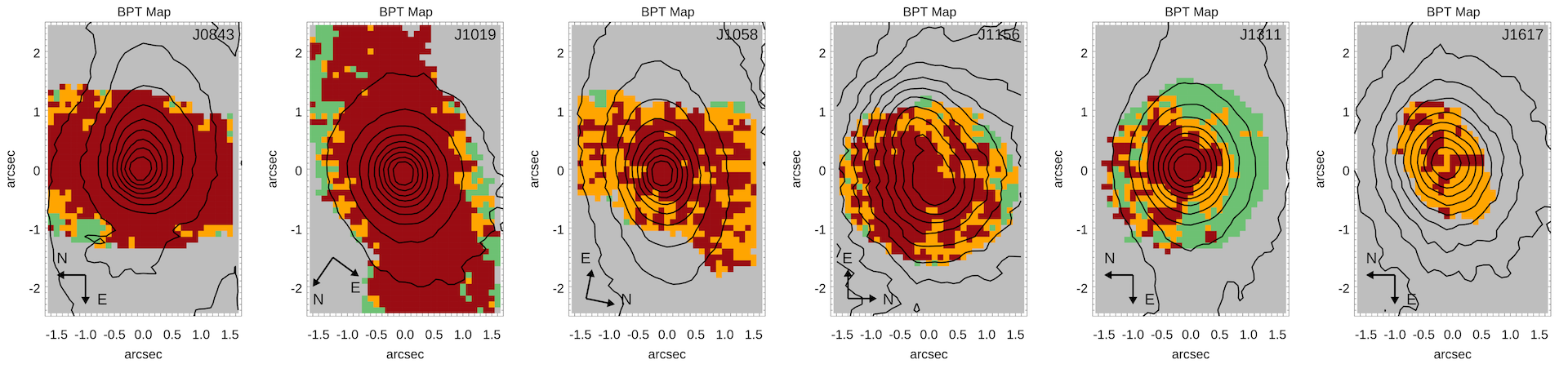
Figure 11.— BPT classification maps. As in Fig. 4, black contours indicate the the stellar continuum flux at 10% intervals from the peak. Gray spaxels indicate spaxels without classification due to weak or non-detection of the emission lines (i.e., S/N $<$ 3).

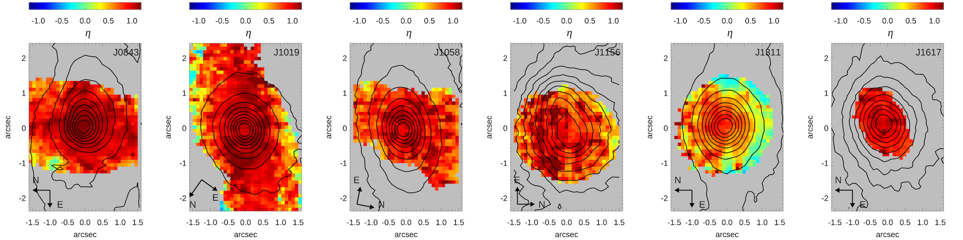
Figure 12.— Photoionization classification maps. We define the $\eta$ parameter following the scenario of Erroz-Ferrer et al. (2019) and use different colors to indicate its value across the galaxies. As in Fig. 4, black contours indicate the the stellar continuum flux at 10% intervals from the peak. Gray spaxels indicate spaxels without classification due to weak or non-detection of the emission lines (i.e., S/N $<$ 3).

4.4.1 Spatially resolved BPT diagram

By combining the flux ratios of [O iii]/H$\beta$ and [N ii]/H$\alpha$, we present the Baldwin, Phillips, & Terievich (BPT) diagram (Baldwin et al., 1981; Veilleux & Osterbrock, 1987) to investigate the source of ionization. We adopt the criteria from Kewley et al. (2001) and Kauffmann et al. (2003) to classify the AGN, composite, and star-forming regions. For dividing Seyfert and LINER regions, we use the demarcation of Cid Fernandes et al. (2010). In Fig. 10, we present the BPT classification of each spaxel as a function of distance from the center. Note that we measure the flux of each emission line using the best-fitted total line profile. We employ a S/N limit of 3 for the [O iii], [N ii] and H$\alpha$ emission lines, whereas we relax the S/N limit to 1 for the H$\beta$ line. Thus, BPT classification is not available in the outer pixels if not all four emission lines are detected. In order to trace the radial change of the [O iii]/H$\beta$ and [N ii]/H$\alpha$ flux ratios, we calculate the mean flux ratios within the distance bin of 0.1 kpc in the projected plane.

In all targets, we observe that the majority of spaxels is classified as Seyfert/LINER region, while there is a clear radial trend from AGN-dominated photoionization toward composite region. This radial change is mainly due to the decrease of the [O iii]/H$\beta$ flux ratio. A significant change of the [N ii]/H$\alpha$ flux ratio is detected in J1019 and J1058, which are the two AGNs with outflows. The origin of this sudden change is unclear and it may be due to the change of gas metallicity or ionization condition.

4.4.2 BPT morphology

In Fig. 11, we present the photoionization classification maps based on the location of spaxels in the BPT diagram. Most targets show AGN-dominated photoionization at the center. In two objects, J1019 and J1311, the AGN-dominated region is surrounded by composite region, which is consistent with our previous finding of a ring-like structure of star-forming region around the AGN-dominated region (Karouzos et al., 2016a; Kang & Woo, 2018).

In order to investigate the spatial change of the line ratios, we introduce the $\eta$ parameter following the scheme of Erroz-Ferrer et al. (2019). We use this parameter to describe the variation of the ionization level, quantifying the contribution from AGN photoionization. $\eta$ is calculated as the orthogonal distance from the bisector of the two demarcation lines: the line between AGN region and composite region (Kewley et al., 2001) and the line between star-forming region and composite region (Kauffmann et al., 2003). We normalize $\eta$ to be equal to 0.5 at the demarcation line of Kewley et al. (2001) and -0.5 at the demarcation line of Kauffmann et al. (2003). In four targets (i.e., J0843, J1019, J1058, J1156), the $\eta$ is greater than 0.5 in most spaxels, in which four emission lines are detected, while the central several kpc area shows the largest $\eta$ value, indicating the dominance of AGN photoionization. The lower $\eta$ in the outer part of the emission regions indicates the decrease of AGN contribution. At the edge of the AGN-dominant region, the $\eta$ becomes lower than 0.5, suggesting a mix of the photoionization from AGN and star-formation. In J1311, AGN photoionization is mainly dominated in the central region, while a ring-like structure with $\eta$ less than 0.5 is present in the circumnuclear region. In the case of J1617, the whole emission region is dominated by the AGN photoionization. As shown in Fig. 11, however, the line flux ratios indicate LINER-like emission except for the central spaxels.

Comparing with the BPT morphology of AGNs with and without strong outflows, we find no significant difference. Based on the BPT morphology of 6 AGNs with strong outflows, Karouzos et al. (2016b) concluded that all objects present the signs of circumnuclear star formation (see also Kang & Woo, 2018). AGNs without strong outflows in our sample also show similar morphology with an AGN-dominant center and a mixing zone of AGN and star-formation. Due to the lack of enough S/N ratios in the outer part of the FOV, it is difficult to conclude whether the ring-like structure of star-forming region is present for all targets, while J1311 is a clear case, which is similar to AGNs with strong outflows studied by Karouzos et al. (2016a).

5. Discussion

Based on the spatially resolved kinematics, we detected the presence of weak outflows in two out of six AGNs in our sample, while no strong signature of outflows was detected in all six objects based on the single-aperture SDSS spectra. Note that this sample has been selected with the same [O iii] luminosity limit along with similar stellar mass and host galaxy inclination in comparison with AGNs with strong outflows in our previous IFU studies (Karouzos et al., 2016a; Kang & Woo, 2018). We discuss the condition and detectability of AGN outflows to understand why some luminous AGNs show no strong outflows.

5.1. Conditions for the presence of outflows

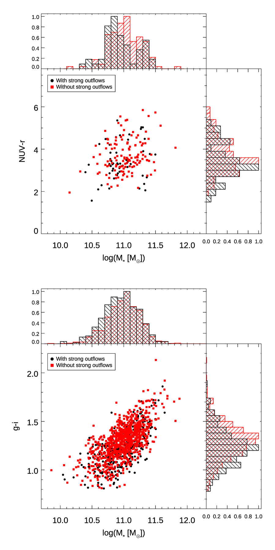
Figure 13.— Distribution of $\mbox{NUV}-r$ color (top), $g-i$ color (bottom) and stellar mass for AGNs with and without strong outflows (black and red colors, respectively).

One of the key conditions for driving outflows is the gas content in the host galaxies. We investigate the cold gas mass fraction using two samples of AGNs, respectively, with and without strong outflows. We use the same sample of the local Type 2 AGNs ($\sim$ 39,000 targets at z $<$ 0.3) in Woo et al. (2016), from which our IFU sample was selected. Following selection criteria are applied: (1) We focus on the AGNs with high luminosity, i.e., $L_{\mathrm{\mbox{[O\,{iii}]};cor}}$ ($>10^{42}$ erg s^-1); (2) To ensure strong outflows, we require the [O iii] velocity shift $|v_{\mbox{[O\,{iii}]}}|>200$ km s^-1 and [O iii] velocity dispersion $\sigma_{\mbox{[O\,{iii}]}}>350$ km s^-1; (3) For the AGNs without strong outflows, we limit the [O iii] velocity shift $|v_{\mbox{[O\,{iii}]}}|<50$ km s^-1 and [O iii] velocity dispersion is consistent with stellar velocity dispersion within 20%. As a result, we obtain 383 AGNs with strong outflows and 1051 AGNs without strong outflows, respectively.

Due to the lack of the multi-wavelength observations to measure gas fraction, we estimate the gas mass fraction by adopting the photometric technique (e.g. Kannappan 2004; Eckert et al. 2015), which uses a broad-band color as a proxy for the cold gas mass fraction. Since our targets are Type 2 AGNs, the galaxy colors will not be significantly affected by the AGN continuum. If any, the effect of AGN on galaxy colors will be similar between two samples. Following the calibration by Eckert et al. (2015), we use the $g-i$ color to derive the HI gas fraction [$M_{HI}/M_{*}$] as

$$log(M_{HI}/M_{*})=-0.984(2.444(g-i)+0.550(b/a))+1.881,$$ (2)

where $g-i$ is limited between 0.8 and 2.6 magnitude, and $b/a$ is the axis ratio of the galaxy. As described in Eckert et al. (2015), the scatter of photometric gas fraction calibration is minimized by including $b/a$ in Equation (2). In the case of the molecular gas fraction [$M_{H_{2}}/M_{*}$], we use the $\mbox{NUV}-r$ color and the scaling relation by Saintonge et al. (2011),

$$log(M_{H_{2}}/M_{*})=-0.293(\mbox{NUV}-r-3.5)-1.349.$$ (3)

Note that these two calibrations have substantial scatter, which introduces relatively large systematic uncertainties in the derived gas fraction. Based on the scatter shown in Eckert et al. (2015) and Saintonge et al. (2011), we estimate that the systematic uncertainty is a factor of 2 for the gas fraction.

In Fig. 13, we compare the distributions of $\mbox{NUV}-r$ color and $g-i$ color with the stellar mass distribution for the selected AGNs with and without strong outflows. We find that the $\mbox{NUV}-r$ color distribution is not significantly different between the two samples, for given the small sample size. In the case of the $g-i$ color, the distribution is somewhat different, showing on average redder $g-i$ color for AGNs without strong outflows, while the stellar mass distribution of the two samples is comparable.

In Fig. 14, we present the calculated gas mass fraction using Eq. 1 and 2. For the molecular gas fraction, we find no significant difference with the mean fraction of $0.055\pm 0.031$ and $0.045\pm 0.022$, respectively for AGNs with and without strong outflows. A two-sample Kolmogorov-Smirnov (KS) test also fails to reject the null hypothesis (with a probability $p=0.017$) that the two samples are drawn from the same parent distribution.

In the case of HI gas, the average gas fraction is comparable between the AGNs with and without strong outflows, with the mean fraction of $0.055\pm 0.058$ and $0.039\pm 0.045$, respectively. However, the KS test rejects the null hypothesis that the two samples are drawn from the same parent distribution at a probability value of $p=1.03\times 10^{-7}$. This is due to the overall difference in the shape of the distribution. This result may suggests that AGNs with and without strong outflows have different distributions of HI gas fraction, implying that the detection of outflows is related to the HI gas content. Since the photometric gas fraction technique has large systemic uncertainties and should be applied to a large sample for statistical analysis, direct measurements of gas fraction in individual galaxies based on HI and CO observations are required, in order to confirm that HI gas fraction is the key for detecting AGN-driven outflows. Following up studies with multi-wavelength data will provide better constrains on the connection between cold gas fraction and AGN outflows.

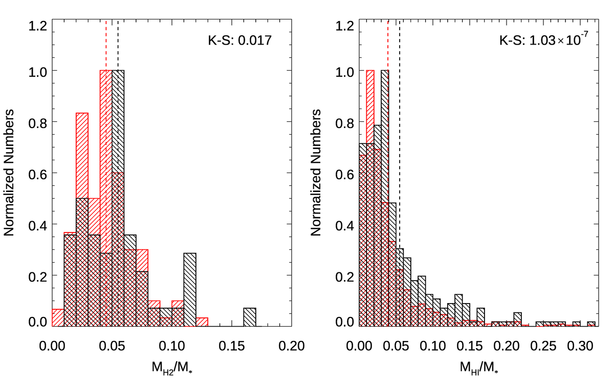
Figure 14.— Distribution of molecular gas fraction (left) and the HI gas fraction (right), based on broad-band colors, for AGNs with and without strong outflows (black and red colors, respectively). The mean gas fraction of each sample is denoted with a dotted line, and the p-value of a two-sample K-S test is given at the upper-right corner

5.2. Outflow detectability

Kpc-scale ionized gas outflows are frequently observed in luminous AGNs, although the outflow fraction varies depending on the definition of outflows. Based on a large sample of $\sim$ 39,000 Type 2 AGNs, Woo et al. (2016) adopted the non-gravitational kinematic signature (i.e. $\sigma_{\mbox{[O\,{iii}]}}>\sigma_{\ast}$) to identify gas outflows, finding that the outflow fraction is at least $\sim$50% over the large dynamic range of [OIII] luminosity, while there is a strong increase of outflow fraction as a function of luminosity, reaching over 80% at $L_{\mathrm{\mbox{[O\,{iii}]}}}>10^{42}$ erg s^-1. By using the similar analysis method, Rakshit & Woo (2018) performed a census of ionized gas outflows using a large sample of Type 1 AGNs ($\sim$ 5000 targets at z $<$ 0.3), reporting that the outflow fraction of Type 1 AGNs is $\sim$90%. As Type 1 AGNs have higher luminosity, these two results consistently indicate a high outflow fraction in luminous AGNs. Similarly, Sun et al. (2017) set a constrain on the outflow fraction of more luminous Type 2 AGNs (i.e., $L_{bol}\gtrsim 10^{46}$ erg s^-1), reporting a $>60\%$ and possibly $\sim 90\%$ occurrence rate. The high occurrence rate of gas outflow indicates that it can persist for a relative long timescale, which has been predicted in the theoretical model of AGN-driven outflows (King et al., 2011). As proposed by Sun et al. (2017), short-term AGN variability over a long-term AGN episode with a moderate AGN duty cycle is a possible scenario to explain the above high outflow occurrence rate.

Since the outflow fraction is very high for luminous AGNs, it may be naively expected that for the relatively luminous AGNs in our sample, the spatially resolved study could reveal AGN-driven outflows, although we did not find signatures of outflows based on the SDSS spectra. However, we detect weak outflow signatures only in two targets out of six AGNs. While we find a hint of difference in HI gas fraction between AGNs with and without outflows, it remains unclear what determines the outflow occurrence.

The structure of outflows and the viewing angle can influence the outflow detectability. As described in the 3D biconical outflow models of Bae & Woo (2016), several structure parameters (e.g. bicone inclination, dust plane inclination, bicone opening angle and dust extinction) can affect the observed gas kinematics (e.g. [O iii] velocity and velocity dispersion) in the projected plane. If the outflow direction is almost perpendicular to the line-of-sight, then the projected velocity shift with respect to the systemic velocity would be minimized, while the velocity dispersion will be relatively small in the line-of-sight if the opening angle of the outflows is small (Bae & Woo, 2016). The intrinsic nature of outflows is yet to be understood except for the outflows in very nearby Seyfert galaxies, for which much higher spatial resolution was possible. More detailed comparison of spatially resolved data with the kinematical models is required to better understand the detectability of ionized gas outflows.

6. Summary

For a sample of six local (z $<$ 0.1) and luminous (L${}_{\mathrm{[OIII]}}>10^{42}$ erg s^-1) Type 2 AGNs, which were selected as AGNs without strong signature of outflows from a large sample of $\sim$39,000 Type 2 AGNs, we performed Gemini/GMOS-IFU observations to investigate the spatially resolved kinematics and the presence of outflows. We summarize the main results as below.

• Ionized gas kinematics in our sample are governed by various physical processes, including merging, AGN-driven outflows and host galaxy gravitational potential. In two targets (i.e., J1019 and J1058), we find significant difference of the kinematics between ionized gas and stars, which can be explained by AGN-driven outflows.

• Based on the spatially resolved kinematics, we find kinematic signatures of outflows for two AGNs (i.e., J1019 and J1058), while the integrated SDSS spectra show no significant outflow signature. The VVD diagram of these two ANGs is consistent with the prediction of outflow kinematics. However, velocity and velocity dispersion of outflows are relatively low, suggesting weak outflows. These results suggest that the outflow fraction derived using integrated spectra can be underestimated, highlighting the importance of spatially-resolved observation in identifying signatures of AGN-driven outflows.

• While the central part is dominated by AGN photoionization, we find a signature of mixing from AGN and star-formation at the edge of the emission region in four AGNs (J0843, J1019, J1058, J1156). One AGN (J1311) clearly shows a ring-like structure of star forming region.

• Based on the indirect estimates of HI gas fraction estimated with the $g-i$ color, we find a hint of the difference in the HI gas fraction between AGNs with and without strong outflows. This result implies that the presence of outflows may depend on the gas fraction.

Appendix A J084344+354942

At z = 0.0541, the GMOS FOV of J0843 covers a $3.6\times 5.4$ kpc region with a spatial resolution of 0.7 kpc. J0843 appears as a merging galaxy with tidal features. [O iii] emission is detected (with S/N $>$ 3) in the central $3.6\times 2.6$ kpc region, while H$\alpha$ emission is more extended. The stellar velocity map shows a velocity gradient in the NW-SE direction. The ionized gas velocity map is complex, probably disturbed by the merging process. As shown in the BPT classification map, AGN photoionization is dominated in the area with significant detection of emission lines, while there are signatures of LINER emission and star-formation at the edge.

Appendix B J101936+193313

At z = 0.0647, the GMOS FOV of J1019 covers a $4.3\times 6.4$ kpc region with a spatial resolution of $0.83$ kpc. With the axis ratio b/a=0.60, J1019 appears as a slightly inclined disk galaxy elongated in the N-S direction. [O iii] and H$\alpha$ emission present a similar spatial distribution with a symmetric shape along the NE-SW direction. The stellar velocity map reveals a clear rotation pattern with the kinematic major axis along the NE-SW direction. The gas velocity map shows an opposite trend compared to that of stars, possibly suggesting a counter-rotation. The bi-conical outflows driven by AGNs is consistent with the observed gas kinematics, if the outflow is along the kinematic major axis. As shown in the BPT classification map, AGN photoionization is dominant, while there are signatures of LINER emission and star-formation at the edge of the emission line region.

Appendix C J105833+461604

At z = 0.0397, the GMOS FOV of J1058 covers a $2.7\times 4.0$ kpc region with a spatial resolution of 0.53 kpc. J1058 is a face-on disk galaxy with a b/a=0.89 along with a clear bar structure. H$\alpha$ emission (with S/N $>$ 3) is distributed in the central $2.7\times 2.9$ kpc region, which is more extended than the distribution of [O iii] emission. The stellar velocity map reveals a rotation pattern. The kinematic major axis of the ionized gas is misaligned with respect to that of the stars by 40 degree, which could be due to the bi-conical outflows driven by AGN. The BPT classification map shows AGN dominated photoionization, while LINER emission is detected at the edge of the emission line region.

Appendix D J115657+550821

At z = 0.0800, the GMOS FOV of J1156 covers a $5.3\times 8.0$ kpc region with a spatial resolution of $1.6$ kpc. J1156 is a face-on disk galaxy with b/a= 0.84. [O iii] and H$\alpha$ emission is concentrated within the $4.0$ kpc region. The stellar velocity map shows no clear rotation pattern while the gas velocity map shows positive (redshifted) velocities, which may be signatures of outflows, but the velocity and velocity dispersion of the ionized gas are relatively small. AGN photoionization is dominant at the center, while there are signatures of LINER emission and star-formation at the edge of the emission line region.

Appendix E J131153+053138

At z = 0.0873, the GMOS FOV of J1311 covers a $5.8\times 8.7$ kpc region with a spatial resolution of $1.1$ kpc. With b/a= 0.85, J1311 appears as a face-on disk galaxy with an outer ring structure. [O iii] emission is centrally concentrated in the 4 kpc region. In contrast, H$\alpha$ emission is more extended, including a bright central component and a weak flux region, that is reaching out to the edge of the FOV. The stellar velocity map reveals a rotation pattern with the kinematic major axis along the E-W direction. The H$\alpha$ velocity map is similar to the stellar velocity map, while the [O iii] velocity map is dominated by positive (redshifted) velocities, which could be due to the AGN-driven outflows. However, [O iii] velocity is relatively small, particularly at the center. As shown in the BPT classification map, the AGN photoionization is dominated in the central region, while there is a ring-like structure of star-forming region at the edge.

Appendix F J161756+221943

At z = 0.1020, the GMOS FOV of J1617 covers a $6.8\times 10.3$ kpc region with a spatial resolution of $2$ kpc. With b/a= 0.85, J1617 appears as a face-on disk galaxy. [O iii] emission is concentrated within the central 2 kpc region, while H$\alpha$ emission is more extended. The stellar velocity map reveals a rotation pattern with the kinematic major axis along the NW-SE direction. The gas velocity map is similar to the stellar velocity map, showing a similar rotation pattern. The BPT classification map shows AGN dominated photoionization.

References

- Alexander & Hickox (2012) Alexander, D. M., & Hickox, R. C. 2012, New Astronomy Reviews, 56, 93, doi: 10.1016/j.newar.2011.11.003
- Bae & Woo (2014) Bae, H.-J., & Woo, J.-H. 2014, ApJ, 795, 30, doi: 10.1088/0004-637X/795/1/30
- Bae & Woo (2016) —. 2016, ApJ, 828, 97, doi: 10.3847/0004-637X/828/2/97
- Bae et al. (2017) Bae, H.-J., Woo, J.-H., Karouzos, M., et al. 2017, ApJ, 837, 91, doi: 10.3847/1538-4357/aa5f5c
- Baldwin et al. (1981) Baldwin, J. A., Phillips, M. M., & Terlevich, R. 1981, Publications of the Astronomical Society of the Pacific, 93, 5, doi: 10.1086/130766
- Belfiore et al. (2016) Belfiore, F., Maiolino, R., Maraston, C., et al. 2016, MNRAS, 461, 3111, doi: 10.1093/mnras/stw1234
- Cappellari & Emsellem (2004) Cappellari, M., & Emsellem, E. 2004, Publications of the Astronomical Society of the Pacific, 116, 138, doi: 10.1086/381875
- Chen et al. (2016) Chen, Y.-M., Shi, Y., Tremonti, C. A., et al. 2016, Nature Communications, 7, 13269, doi: 10.1038/ncomms13269
- Cicone et al. (2012) Cicone, C., Feruglio, C., Maiolino, R., et al. 2012, A&A, 543, A99, doi: 10.1051/0004-6361/201218793
- Cid Fernandes et al. (2010) Cid Fernandes, R., Stasińska, G., Schlickmann, M. S., et al. 2010, MNRAS, 403, 1036, doi: 10.1111/j.1365-2966.2009.16185.x
- Corsini (2014) Corsini, E. M. 2014, in Multi-Spin Galaxies, ed. E. Iodice & E. M. Corsini, Vol. 486, 51
- Croton et al. (2006) Croton, D. J., Springel, V., White, S. D. M., et al. 2006, MNRAS, 365, 11, doi: 10.1111/j.1365-2966.2005.09675.x
- Davies et al. (2014) Davies, R. I., Maciejewski, W., Hicks, E. K. S., et al. 2014, ApJ, 792, 101, doi: 10.1088/0004-637X/792/2/101
- Di Matteo et al. (2005) Di Matteo, T., Springel, V., & Hernquist, L. 2005, Nature, 433, 604, doi: 10.1038/nature03335
- Dumas et al. (2007) Dumas, G., Mundell, C. G., Emsellem, E., & Nagar, N. M. 2007, MNRAS, 379, 1249, doi: 10.1111/j.1365-2966.2007.12014.x
- Eckert et al. (2015) Eckert, K. D., Kannappan, S. J., Stark, D. V., et al. 2015, ApJ, 810, 166, doi: 10.1088/0004-637X/810/2/166
- Elvis (2000) Elvis, M. 2000, ApJ, 545, 63, doi: 10.1086/317778
- Erroz-Ferrer et al. (2019) Erroz-Ferrer, S., Carollo, C. M., den Brok, M., et al. 2019, arXiv e-prints, https://arxiv.org/abs/1901.04493
- Fabian (2012) Fabian, A. C. 2012, Annual Review of Astronomy and Astrophysics, 50, 455, doi: 10.1146/annurev-astro-081811-125521
- Falcón-Barroso et al. (2011) Falcón-Barroso, J., Sánchez-Blázquez, P., Vazdekis, A., et al. 2011, A&A, 532, A95, doi: 10.1051/0004-6361/201116842
- Ferrarese & Merritt (2000) Ferrarese, L., & Merritt, D. 2000, ApJ, 539, L9, doi: 10.1086/312838
- Feruglio et al. (2010) Feruglio, C., Maiolino, R., Piconcelli, E., et al. 2010, A&A, 518, L155, doi: 10.1051/0004-6361/201015164
- Gebhardt et al. (2000) Gebhardt, K., Bender, R., Bower, G., et al. 2000, ApJ, 539, L13, doi: 10.1086/312840
- Genzel et al. (2014) Genzel, R., Förster Schreiber, N. M., Rosario, D., et al. 2014, ApJ, 796, 7, doi: 10.1088/0004-637X/796/1/7
- Harrison et al. (2012) Harrison, C. M., Alexander, D. M., Mullaney, J. R., et al. 2012, ApJ, 760, L15, doi: 10.1088/2041-8205/760/1/L15
- Heckman & Best (2014) Heckman, T. M., & Best, P. N. 2014, Annual Review of Astronomy and Astrophysics, 52, 589, doi: 10.1146/annurev-astro-081913-035722
- Ho (2008) Ho, L. C. 2008, Annual Review of Astronomy and Astrophysics, 46, 475, doi: 10.1146/annurev.astro.45.051806.110546
- Hopkins et al. (2006) Hopkins, P. F., Hernquist, L., Cox, T. J., et al. 2006, The Astrophysical Journal Supplement Series, 163, 1, doi: 10.1086/499298
- Husemann et al. (2012) Husemann, B., Kamann, S., Sandin, C., et al. 2012, A&A, 545, A137, doi: 10.1051/0004-6361/201220102
- Jin et al. (2016) Jin, Y., Chen, Y., Shi, Y., et al. 2016, MNRAS, 463, 913, doi: 10.1093/mnras/stw2055
- Kang & Woo (2018) Kang, D., & Woo, J.-H. 2018, ArXiv e-prints, arXiv:1807.08356. https://arxiv.org/abs/1807.08356
- Kang et al. (2017) Kang, D., Woo, J.-H., & Bae, H.-J. 2017, ApJ, 845, 131, doi: 10.3847/1538-4357/aa80e8
- Kannappan (2004) Kannappan, S. J. 2004, ApJ, 611, L89, doi: 10.1086/423785
- Karouzos et al. (2016a) Karouzos, M., Woo, J.-H., & Bae, H.-J. 2016a, ApJ, 819, 148, doi: 10.3847/0004-637X/819/2/148
- Karouzos et al. (2016b) —. 2016b, ApJ, 833, 171, doi: 10.3847/1538-4357/833/2/171
- Kauffmann et al. (2003) Kauffmann, G., Heckman, T. M., Tremonti, C., et al. 2003, MNRAS, 346, 1055, doi: 10.1111/j.1365-2966.2003.07154.x
- Kewley et al. (2001) Kewley, L. J., Dopita, M. A., Sutherland, R. S., Heisler, C. A., & Trevena, J. 2001, ApJ, 556, 121, doi: 10.1086/321545
- Kewley et al. (2006) Kewley, L. J., Groves, B., Kauffmann, G., & Heckman, T. 2006, MNRAS, 372, 961, doi: 10.1111/j.1365-2966.2006.10859.x
- King et al. (2011) King, A. R., Zubovas, K., & Power, C. 2011, MNRAS, 415, L6, doi: 10.1111/j.1745-3933.2011.01067.x
- Kormendy & Ho (2013) Kormendy, J., & Ho, L. C. 2013, Annual Review of Astronomy and Astrophysics, 51, 511, doi: 10.1146/annurev-astro-082708-101811
- Li et al. (2015) Li, Z., Shen, J., & Kim, W.-T. 2015, ApJ, 806, 150, doi: 10.1088/0004-637X/806/2/150
- Lintott et al. (2011) Lintott, C., Schawinski, K., Bamford, S., et al. 2011, MNRAS, 410, 166, doi: 10.1111/j.1365-2966.2010.17432.x
- Liu et al. (2013a) Liu, G., Zakamska, N. L., Greene, J. E., Nesvadba, N. P. H., & Liu, X. 2013, MNRAS, 430, 2327, doi: 10.1093/mnras/stt051
- Liu et al. (2013b) Liu, G., Zakamska, N. L., Greene, J. E., Nesvadba, N. P. H., & Liu, X. 2013, MNRAS, 436, 2576, doi: 10.1093/mnras/stt1755
- Maiolino et al. (2012) Maiolino, R., Gallerani, S., Neri, R., et al. 2012, MNRAS, 425, L66, doi: 10.1111/j.1745-3933.2012.01303.x
- Markwardt (2009) Markwardt, C. B. 2009, in Astronomical Data Analysis Software and Systems XVIII, ed. D. A. Bohlender, D. Durand, & P. Dowler, Vol. 411, 251
- Marquardt (1963) Marquardt, D. W. 1963, Journal of the Society for Industrial and Applied Mathematics, 11, 431
- McElroy et al. (2015) McElroy, R., Croom, S. M., Pracy, M., et al. 2015, MNRAS, 446, 2186, doi: 10.1093/mnras/stu2224
- Moré (1978) Moré, J. 1978, in Lecture Notes in Mathematics, Vol. 630, Numerical Analysis, ed. G. Watson (Springer Berlin Heidelberg), 105–116
- Mullaney et al. (2013) Mullaney, J. R., Alexander, D. M., Fine, S., et al. 2013, MNRAS, 433, 622, doi: 10.1093/mnras/stt751
- Nesvadba et al. (2008) Nesvadba, N. P. H., Lehnert, M. D., De Breuck, C., Gilbert, A. M., & van Breugel, W. 2008, A&A, 491, 407, doi: 10.1051/0004-6361:200810346
- Rakshit & Woo (2018) Rakshit, S., & Woo, J.-H. 2018, ArXiv e-prints, arXiv:1808.03415. https://arxiv.org/abs/1808.03415
- Rupke & Veilleux (2013) Rupke, D. S. N., & Veilleux, S. 2013, ApJ, 768, 75, doi: 10.1088/0004-637X/768/1/75
- Saintonge et al. (2011) Saintonge, A., Kauffmann, G., Kramer, C., et al. 2011, MNRAS, 415, 32, doi: 10.1111/j.1365-2966.2011.18677.x
- Sharp & Bland-Hawthorn (2010) Sharp, R. G., & Bland-Hawthorn, J. 2010, ApJ, 711, 818, doi: 10.1088/0004-637X/711/2/818
- Springel et al. (2005) Springel, V., White, S. D. M., Jenkins, A., et al. 2005, Nature, 435, 629, doi: 10.1038/nature03597
- Storchi-Bergmann et al. (2010) Storchi-Bergmann, T., Lopes, R. D. S., McGregor, P. J., et al. 2010, MNRAS, 402, 819, doi: 10.1111/j.1365-2966.2009.15962.x
- Sun et al. (2017) Sun, A.-L., Greene, J. E., & Zakamska, N. L. 2017, ApJ, 835, 222, doi: 10.3847/1538-4357/835/2/222
- Tremaine et al. (2002) Tremaine, S., Gebhardt, K., Bender, R., et al. 2002, ApJ, 574, 740, doi: 10.1086/341002
- Veilleux et al. (2005) Veilleux, S., Cecil, G., & Bland-Hawthorn, J. 2005, Annual Review of Astronomy and Astrophysics, 43, 769, doi: 10.1146/annurev.astro.43.072103.150610
- Veilleux & Osterbrock (1987) Veilleux, S., & Osterbrock, D. E. 1987, The Astrophysical Journal Supplement Series, 63, 295, doi: 10.1086/191166
- Wang et al. (2011) Wang, J., Mao, Y. F., & Wei, J. Y. 2011, ApJ, 741, 50, doi: 10.1088/0004-637X/741/1/50
- Wang et al. (2018) Wang, J., Xu, D. W., & Wei, J. Y. 2018, ApJ, 852, 26, doi: 10.3847/1538-4357/aa9d1b
- Woo et al. (2016) Woo, J.-H., Bae, H.-J., Son, D., & Karouzos, M. 2016, ApJ, 817, 108, doi: 10.3847/0004-637X/817/2/108
- Woo et al. (2017) Woo, J.-H., Son, D., & Bae, H.-J. 2017, ApJ, 839, 120, doi: 10.3847/1538-4357/aa6894
- Woo et al. (2015) Woo, J.-H., Yoon, Y., Park, S., Park, D., & Kim, S. C. 2015, ApJ, 801, 38, doi: 10.1088/0004-637X/801/1/38
- Zhang et al. (2011) Zhang, K., Dong, X.-B., Wang, T.-G., & Gaskell, C. M. 2011, ApJ, 737, 71, doi: 10.1088/0004-637X/737/2/71
- Zhang et al. (2017) Zhang, S., Zhou, H., Shi, X., et al. 2017, ApJ, 836, 86, doi: 10.3847/1538-4357/836/1/86