Load-Balancing for Parallel Delaunay Triangulations

Abstract

Computing the Delaunay triangulation (DT) of a given point set in $\mathbb{R}^{D}$ is one of the fundamental operations in computational geometry. Recently, Funke and Sanders [18] presented a divide-and-conquer DT algorithm that merges two partial triangulations by re-triangulating a small subset of their vertices – the border vertices – and combining the three triangulations efficiently via parallel hash table lookups. The input point division should therefore yield roughly equal-sized partitions for good load-balancing and also result in a small number of border vertices for fast merging. In this paper, we present a novel divide-step based on partitioning the triangulation of a small sample of the input points. In experiments on synthetic and real-world data sets, we achieve nearly perfectly balanced partitions and small border triangulations. This almost cuts running time in half compared to non-data-sensitive division schemes on inputs exhibiting an exploitable underlying structure.

1 Introduction

The Delaunay triangulation (DT) of a given point set in $\mathbb{R}^{D}$ has numerous applications in computer graphics, data visualization, terrain modeling, pattern recognition and finite element methods [22]. Computing the DT is thus one of the fundamental operations in geometric computing. Therefore, many algorithms for efficiently computing the DT have been proposed (see survey in [31]) and well implemented codes exist [19, 28]. With ever increasing input sizes, research interest has shifted from sequential algorithms towards parallel ones [4, 6, 12, 22, 17, 8].

Recently, we presented a novel divide-and-conquer (D&C) DT algorithm for arbitrary dimension [18] that lends itself equally well to shared and distributed memory parallelism and thus hybrid parallelization. While previous D&C DT algorithms suffer from a complex – often sequential – divide or merge step [12, 24], our algorithm reduces the merging of two partial triangulations to re-triangulating a small subset of their vertices – the border vertices – using the same parallel algorithm and combining the three triangulations efficiently via hash table lookups. All steps required for the merging – identification of relevant vertices, triangulation and combining the partial DTs – are performed in parallel.

The division of the input points in the divide-step needs to address a twofold sensitivity to the point distribution: the partitions need to be approximately equal-sized for good load-balancing, while the number of border vertices needs to be minimized for fast merging. This requires partitions that have many internal Delaunay edges but only few external ones, i. e. a graph partitioning of the DT graph. In this paper we propose a novel divide-step that approximates this graph partitioning by triangulating and partitioning a small sample of the input points, and divides the input point set accordingly.

The paper is structured as follows: we review the problem definition, related work on partitioning for DT algorithms and our D&C DT algorithm from [18] in Section 2. Subsequently, our proposed divide-step is described in Section 3, along with a description of fast intersection tests for the more complexly shaped partition borders and implementation notes. We evaluate our algorithms in Section 4 and close the paper with conclusions and an outlook on future work in Section 5.

2 Preliminaries

2.1 Delaunay Triangulations

A $d$-simplex is a generalization of a triangle ($d=2$) to $d$-dimensional space. A $d$-simplex $s$ is a $d$-dimensional polytope, i. e. the convex hull of $d+1$ points. The convex hull of $m+1$ of these $d+1$ points is called an $m$-face of $s$. Specifically, the $0$-faces are the vertices of $s$ and the $(d-1)$-faces are its facets. Given a $d$-dimensional point set $\mathbf{P}=\{p_{1},p_{2},\dots,p_{n}\}\subset\mathbb{R}^{d}$ for all $i\in\{1,\dots,n\}$, a triangulation $T(\mathbf{P})$ is a subdivision of the convex hull of $\mathbf{P}$ into $d$-simplices such that the set of vertices of $T(\mathbf{P})$ coincides with $\mathbf{P}$ and any two simplices of $T$ intersect in a common $d-1$ facet or not at all. The union of all simplices in $T(\mathbf{P})$ is the convex hull of point set $\mathbf{P}$. A Delaunay triangulation $DT(\mathbf{P})$ is a triangulation of $\mathbf{P}$ such that no point of $\mathbf{P}$ is inside the circumhypersphere of any simplex in $DT(\mathbf{P})$. If the points of $\mathbf{P}$ are in general position, i. e. no $d+2$ points lie on a common $d$-hypersphere, $DT(\mathbf{P})$ is unique [14].

2.2 Related Work

Many algorithms for the parallel construction of the DT of a given point set have been proposed in the literature. They generally fall into one of two categories: parallel incremental insertion and D&C approaches. We will focus on a review of the divide-step of the latter. A more comprehensive discussion of both algorithm types is given in [18].

Aggarwal et al. [1] propose the first parallel D&C DT algorithm. They partition the input points along a vertical line into blocks, which are triangulated in parallel and then merged sequentially. The authors do not prescribe how to determine the location of the splitting line. Cignoni et al. [12] partition the input along cutting (hyper)planes and firstly construct the simplices of the triangulation crossing those planes before recursing on the two partitions. The remaining simplices can be created in parallel in the divided regions without further merging. The authors mention that the regions should be of roughly equal cardinality, but do not go into the details of the partitioning. Chen [7] and Lee et al. [24] explicitly require splitting along the median of the input points. Whereas the former uses classical splitting planes, the latter traces the splitting line with Delaunay edges, thus eliminating the need for later merging.

The subject of input partitioning has received more attention in the meshing community. A mesh of a point set $\mathbf{P}$ is a triangulation of every point in $\mathbf{P}$ and possibly more – so called Steiner points – to refine the triangulation [9]. Chrisochoides [10] surveys algorithms for parallel mesh generation and differentiates between continuous domain decomposition – using quad- or oct-trees – and discrete domain decomposition using an initial coarse mesh that is partitioned into submeshes, trying to minimize the surface-to-volume ratio of the submeshes. Chrisochoides and Nave [11] propose an algorithm that meshes the subproblems via incremental insertion using the Bowyer-Watson algorithm.

2.3 Parallel Divide-and-Conquer DT Algorithm

1:points $\mathbf{P}=\{p_{1},\dots,p_{n}\}$ with $p_{i}\in\mathbb{R}^{D}$

2:Delaunay triangulation $DT(\mathbf{P})$

3:if $n<N$ then

4:     return $\operatorname{\emph{sequentialDelaunay}}(\mathbf{P})$ $\triangleright$ base case

5:$\begin{pmatrix}\mathbf{P}_{1}&\dots&\mathbf{P}_{k}\end{pmatrix}\leftarrow\operatorname{partitionPoints}(\mathbf{P},k)$ $\triangleright$ partition points into $k$ partitions

6:$\begin{pmatrix}T_{1}&\dots&T_{k}\end{pmatrix}\leftarrow\begin{pmatrix}\operatorname{Delaunay}(\mathbf{P}_{1})&\dots&\operatorname{Delaunay}(\mathbf{P}_{k})\end{pmatrix}$ $\triangleright$ parallel triangulation

7: Border triangulation:

8:$\mathbf{B}\leftarrow\varnothing;\quad\mathbf{Q}\leftarrow\bigcup_{1\leq i\leq k}\operatorname{convexHull}(T_{i})$ $\triangleright$ initialize set of border simplices

9:parfor $s_{i,x}\in\mathbf{Q}$ do $\triangleright$ simplex originating from triangulation $T_{i}$

10:     $\operatorname{mark}(s_{i,x})$ $\triangleright$ process each simplex only once

11:     if $\operatorname{intersects}\left(\operatorname{circumsphere}(s_{i,x}),T_{j}\right)\text{, with $i\neq j$}$ then

12:         $\mathbf{B}\,\,\cup\!\!=\{s_{i,x}\}$ $\triangleright$ circumsphere intersects other partition, $s_{i,x}$ is border simplex

13:         for $s_{i,y}\in\operatorname{neighbors}(s_{i,x})\wedge\neg\operatorname{marked}(s_{i,y})$ do $\triangleright$ process all neighbors

14:              $\mathbf{Q}\,\,\cup\!\!=s_{i,y};\quad\operatorname{mark}(s_{i,y})$               

15:$T_{B}\leftarrow\operatorname{Delaunay}(\operatorname{vertices}(\mathbf{B}))$ $\triangleright$ triangulate points of border simplices

16: Merging:

17:$T\leftarrow\left(\bigcup_{1\leq i\leq k}T_{k}\right)\setminus\mathbf{B};\quad\mathbf{Q}\leftarrow\varnothing$ $\triangleright$ merge partial triangulations, strip border

18:parfor $s_{b}\in T_{B}$ do $\triangleright$ merge simplices from border triangulation

19:     if $\operatorname{vertices}(s_{b})\not\subset\mathbf{P}_{i}\quad\forall 1\leq i\leq k$ then

20:         $T\,\,\cup\!\!=\{s_{b}\};\quad Q\,\,\cup\!\!=\{s_{b}\}$ $\triangleright$ $s_{b}$ spans multiple partitions

21:     else

22:         if $\exists s\in\mathbf{B}:\operatorname{vertices}(s)=\operatorname{vertices}(s_{b})$ then

23:              $T\,\,\cup\!\!=\{s_{b}\};\quad Q\,\,\cup\!\!=\{s_{b}\}$ $\triangleright$ $s_{b}$ replaces border simplex               

24: Neighborhood update:

25:parfor $s_{x}\in Q$ do $\triangleright$ update neighbors of inserted simplices

26:     for $d\in\{1,\dots,D+1\}$ do

27:         if $\operatorname{neighbors}_{d}(s_{x})\not\in T$ then $\triangleright$ neighbor no longer in triangulation

28:              $C\leftarrow\{s_{c}:f_{d}(s_{x})=f_{d}(s_{c})\}$ $\triangleright$ candidates with same facet hash

29:              for $s_{c}\in C$ do

30:                  if $|\operatorname{vertices}(s_{x})\cap\operatorname{vertices}(s_{c})|=D$  then

31:                       $\operatorname{neighbors}_{d}(s_{x})\leftarrow s_{c};\quad Q\,\,\cup\!\!=s_{c}$ $\triangleright$ $s_{c}$ is neighbor of $s_{x}$                                               

32:return $T$

Algorithm 1 $\operatorname{Delaunay}(\mathbf{P})$: shared memory parallel D&C algorithm

Recently, we presented a parallel divide-and-conquer algorithm for computing the DT of a given point set [18]. Our algorithm recursively divides the input into two partitions which are triangulated in parallel. The contribution lies in a novel merging step for the two partial triangulations which re-triangulates a small subset of their vertices and combines the three triangulations via parallel hash table lookups. For each partial triangulation the border is determined, i. e. the simplices whose circumhypersphere intersects the bounding box of the other triangulation. The vertices of those border simplices are then re-triangulated to obtain the border triangulation. The merging proceeds by combining the two partial triangulations, stripping the original border simplices and adding simplices from the border triangulation iff i) they span multiple partitions; or ii) are contained within one partition but exist in the same form in the original triangulation. We adapt the original algorithm to an arbitrary number of partitions in Algorithm 1.

The algorithm’s sensitivity to the input point distribution is twofold: the partitions need to be of equal size for good load-balancing between the available cores and the number of simplices in the border needs to minimized in order to reduce merging overhead. As presented in [18], the algorithm splits the input into two partitions along a hyperplane. Three strategies to choose the splitting dimension are proposed: i) constant, predetermined splitting dimension; ii) cyclic choice of the splitting dimension – similar to $k$-D trees [5]; or iii) dimension with largest extend. This can lead to imbalance in the presence of non-homogeneously structured inputs, motivating the need for more sophisticated partitioning schemes.

3 Sample-based Partitioning

1:points $\mathbf{P}=\{p_{1},\dots,p_{n}\}$ with $p_{i}\in\mathbb{R}^{D}$, number of partitions $k$

2:partitioning $\begin{pmatrix}\mathbf{P}_{1}&\dots&\mathbf{P}_{k}\end{pmatrix}$

3:$\mathbf{P}_{S}\leftarrow\text{choose $\eta(n)$ from $\mathbf{P}$ uniformly at random}$ $\triangleright$ $\eta(n)$ sample size

4:$T\leftarrow\operatorname{Delaunay}(\mathbf{P}_{S})$

5:$G=(V,E,\omega)$ with $V=\mathbf{P}_{S}$, $E=T$ and weight function $\omega$

6:$\begin{pmatrix}V_{1}&\dots&V_{k}\end{pmatrix}\leftarrow\operatorname{partition}(G)$ $\triangleright$ partition graph

7:$\begin{pmatrix}\mathbf{P}_{1}&\dots&\mathbf{P}_{k}\end{pmatrix}\leftarrow\begin{pmatrix}\varnothing&\dots&\varnothing\end{pmatrix}$

8:parfor $p\in\mathbf{P}$ do

9:     $v_{n}\leftarrow\operatorname*{arg\,min}_{v\in\mathbf{P}_{S}}||p-v||$ $\triangleright$ find nearest sample point to $p$

10:     $\mathbf{P}_{i}\,\,\cup\!\!=p\text{ with }i\in[1\dots k]:v_{n}\in V_{i}$ $\triangleright$ assign $p$ to $v_{n}$’s partition

11:return $\begin{pmatrix}\mathbf{P}_{1}&\dots&\mathbf{P}_{k}\end{pmatrix}$

Algorithm 2 $\operatorname{partitionPoints}(\mathbf{P},k)$: partition input into $k$ partitions.

In this paper, we propose more advanced strategies for partitioning the input points than originally presented in [18]. The desired partitioning addresses both data sensitivities of Algorithm 1. The underlying idea is derived from sample sort [16]: gain insight into the input distribution from a (small) sample of the input. Algorithm 2 describes our partitioning procedure. A sample $\mathbf{P}_{S}$ of $\eta(n)$ points is taken from the input point set of size $n$ and triangulated to obtain $DT(\mathbf{P}_{S})$. A similar approach can be found in Delaunay hierarchies, were the sample triangulation is used to speed up point location queries [15].

Instead, we transform the DT into a graph $G=(V,E,\omega)$, with $V$ being equal to the sample point set $\mathbf{P}_{S}$ and $E$ containing all edges of $DT(\mathbf{P}_{S})$. The resulting graph is then partitioned using a graph partitioning tool to obtain a partition into $k$ blocks.

The choice of weight function $\omega$ influences the quality of the resulting partitioning. As mentioned in Section 2.3, the D&C algorithm is sensitive to the balance of the blocks as well as the size of the border triangulation. The former is ensured by the imbalance parameter $\epsilon$ of the graph partitioning, which guarantees that for all partitions $i$: $\left|V_{i}\right|\leq(1+\epsilon)\lceil\frac{|V|}{k}\rceil$. The latter needs to be addressed by the edge weight function $\omega$ of the graph. In order to minimize the size of the border triangulation, dense regions of the input points should not be cut by the partitioning. Sparse regions of the input points result in long Delaunay edges in the sample triangulation. As graph partitioning tries to minimize the weight of the cut edges, edge weights need to be inversely related to the Euclidean length of the edge. Table 1 provides an overview of the edge weight functions considered, which are evaluated in Section 4.1.

Given the partitions of the sample vertices $(V_{1}\dots V_{k})$, the partitioning needs to be extended to the entire input point set. The dual of the Delaunay triangulation of the sample point set – its Voronoi diagram – defines a partitioning of the Euclidean space $\mathbb{R}^{d}$ in the following sense: each point $p_{S,i}$ of the sample is assigned to a partition $j\in[1\dots k]$. Accordingly, its Voronoi cell with respect to $\mathbf{P}_{S}$ defines the sub-space of $\mathbb{R}^{d}$ associated with partition $j$. In order to extend the partitioning to the entire input point set, each point $p\in\mathbf{P}$ is assigned to the partition of its containing Voronoi cell.

All steps in Algorithm 2 can be efficiently parallelized. Sanders et al. [27] present an efficient parallel random sampling algorithm. The triangulation of the sample point set $\mathbf{P}_{S}$ could be computed in parallel using our DT algorithm recursively. However, as the sample is small, a fast sequential algorithm is typically more efficient. Graph conversion is trivially done in parallel and Akhremtsev et al. [3] present a parallel graph partitioning algorithm. The parallelization of the assignment of input points to their respective partitions is explicitly given in Algorithm 2.

Weight	$\mathbf{\bm{\omega}(e=(v,w)}$
constant	1
inverse	$\frac{1}{d(v,w)}$
logarithmic	$-\log d(v,w)$
linear	$1-d(v,w)$

Table 1: Possible choices for the edge weight $\omega$, with $d(v,w)=\frac{||v-w||}{d^{\ast}}$ denoting the normalized Euclidean distance of points $v$ and $w$, with $d^{\ast}$ being the length of the maximum diagonal.

3.1 Recursive Bisection & Direct $k$-way Partitioning

Two possible strategies exist to obtain $k$ partitions from a graph: direct $k$-way partitioning and recursive bisection. For the latter, the graph is recursively partitioned into $k^{\prime}=2$ partitions $\log k$ times. In the graph partitioning community, Simon and Teng [30] prove that recursive bisection can lead to arbitrarily bad partitions and Kernighan and Lin [21] confirm the superiority of direct $k$-way partitioning experimentally. However, recursive bisection is still widely – and successfully – used in practice (e. g. in METIS [20] and for initial partitioning in KaHIP [26]). Other problem domains also apply recursive bisection successfully. In hypergraph partitioning, it can lead to better partitionings in the presence of large hyperedges, i. e. edges with many vertices [2]. We therefore consider both partitioning variants for obtaining $k$ partitions for our DT algorithm.

The partitioning schemes originally proposed in [18] can be seen as recursive bisection: the input is recursively split along the median. The splitting dimension is chosen in a cyclic fashion, similiar to $k$-D trees. Figure 1(a) shows an example.

Similarly, Algorithm 2 can be applied $\log k$ times, at each step $i$ drawing a new sample point set $\mathbf{P}_{S,i}$, triangulating and partitioning $\mathbf{P}_{S,i}$, and assigning the remaining input points to their respective partition. As in the original scheme, this leads to $k-1$ merge steps, entailing $k-1$ border triangulations. In the sample-based approach however, the partitioning avoids cutting dense regions of the input, which would otherwise lead to large and expensive border triangulations; refer to Figure 1(c).

Using direct $k$-way partitioning, only one partitioning and one merge step is required. The single border point set will be larger, with points spread throughout the entire input area. This however, allows for efficient parallelization of the border triangulation step using our DT algorithm recursively. Figure 1(b) depicts an example partitioning.

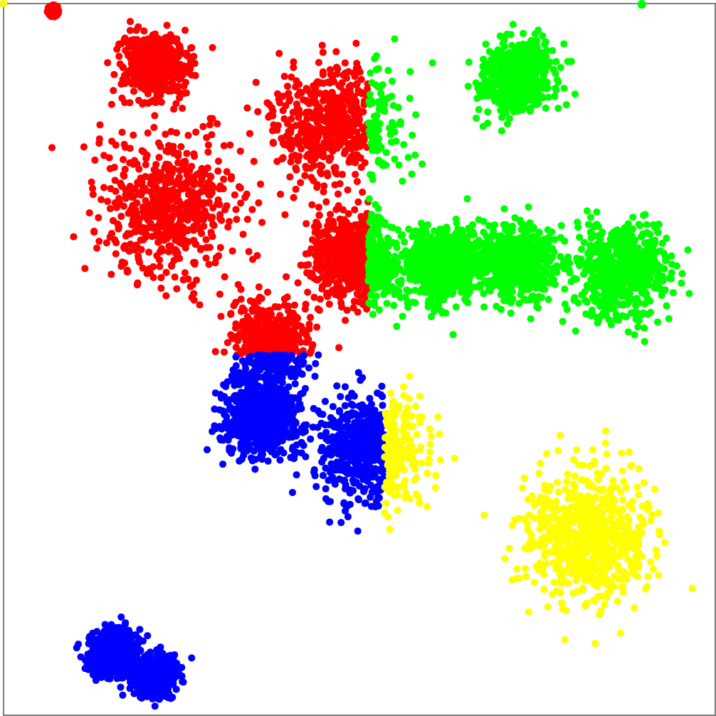
(a) cycle

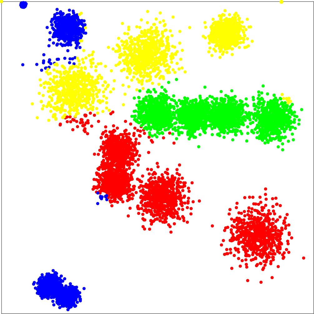
(b) direct $k$-way

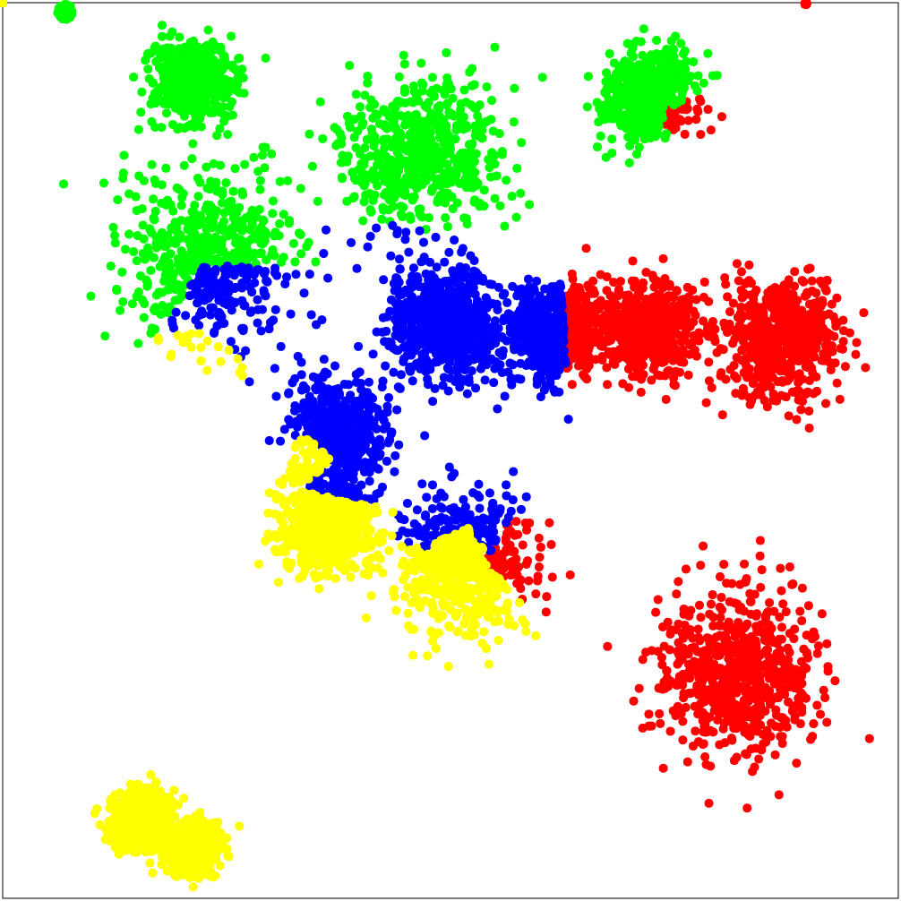
(c) recursive bisection

Figure 1: Example for two-dimensional partitioning with $10\,000$ points and a sample size of $1000$.

3.2 Geometric Primitives

Our D&C algorithm [18] mostly relies on combinatorial computations on hash values except for the base case computations and the detection of the border simplices. The original partitioning schemes always result in partitions defined by axis-aligned bounding boxes. Therefore, the intersection test in Line 11 in Algorithm 1 can be performed using the fast box-sphere overlap test of Larsson et al. [23]. However, using the more advanced partitioning algorithms presented in this paper, this is no longer true. Therefore the geometric primitives to determine the border simplices need to be adapted to the more complexly shaped partitions. The primitives need to balance the computational cost of the intersection test itself with the associated cost for including non-essential points in the border triangulation.

(a) bounding box

(b) grid-based

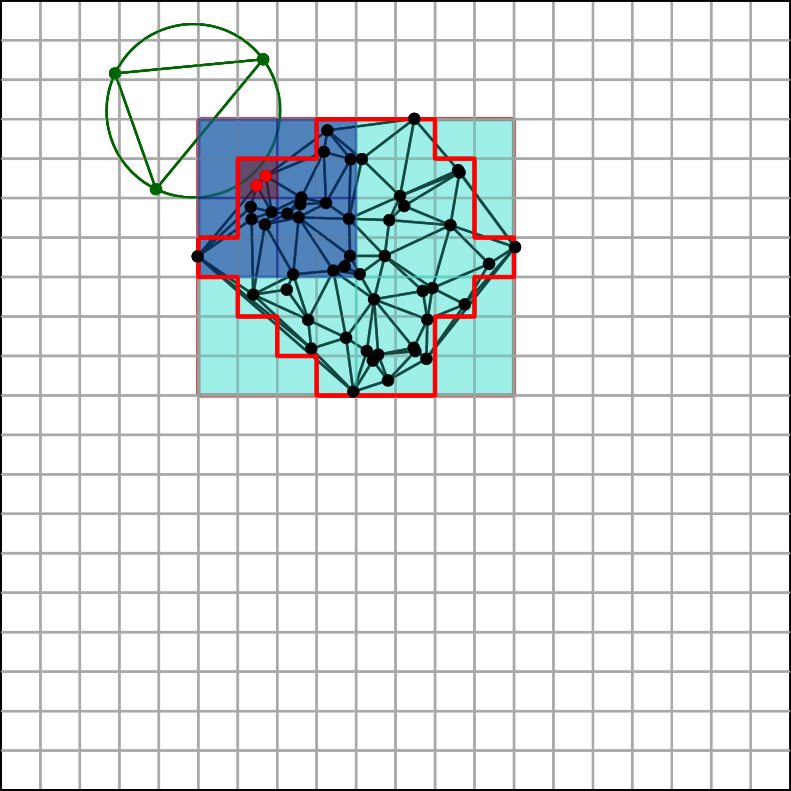
(c) exact

Figure 2: Partition boundary determination strategies. The path through the AABB tree to test for intersection with the circle in the upper left is marked by the colored squares. The tested points for the exact strategy are highlightes in red.

3.2.1 Bounding Box Intersection Test

A crude approximation uses the bounding box of each partition and the fast intersection test of Larsson et al. [23] to determine the simplices that belong to the border of a partition. While computationally cheap, the bounding box can overestimate the extent of a partition. Figure 2(a) provides an example.

3.2.2 Grid-based Intersection Test

To improve accuracy while still keeping the determination of the border simplices geometrically simple and computationally cheap, we use a uniform grid combined with an AABB tree [32]. For each partition $\mathbf{P}_{k}$ it is determined which cells of the uniform grid $\mathcal{G}$ are occupied by points from that partition, i. e., $\mathbf{\mathcal{C}}_{k}=\left\{c\in\mathcal{G}:\exists p\in\mathbf{P}_{k}:p\in c\right\}$. To accelerate the intersection tests we build an AABB tree on top of each set $\mathbf{\mathcal{C}}_{k}$, depicted in Figure 2(b). The AABB tree is built once for every partition $k$ and contains the occupied grid cells $\mathbf{\mathcal{C}}_{k}$ as leaves and recursively more coarse-grained bounding boxes. The root node of the tree corresponds to the bounding box from Section 3.2.1. This allows for a more accurate test whether a given simplex $s$ of partition $i$ intersects with partition $j$ using $\log|\mathbf{\mathcal{C}}_{j}|$ box-sphere intersection tests [23].

3.2.3 Exact Intersection Test

In order to only add the absolutely necessary points to the border triangulation an even more computationally expensive test is required. For a given simplex $s$ of partition $i$ we use the AABB intersection test from the previous section to determine the set $\mathbf{\mathcal{C}}^{\prime}_{j}\subseteq\mathbf{\mathcal{C}}_{j}$ of cells intersected by the circumhypersphere of $s$ in partition $j$. For all points contained in these cells an adaptive precision inSphere-test [29] is performed to determine whether $s$ violates the Delaunay property and thus its vertices need to be added to the border triangulation.

3.3 Implementation Notes

We integrated our divide-step into the implementation of [18], which is available as open source. We use KaHIP [26] and its parallel version [3] as graph partitioning tool. The triangulation of the sample point set is computed sequentially using CGAL [19] with exact predicates. The closest sample point for a given input point in Line 10 of Algorithm 2 can be found via the Voronoi diagram of the sample triangulation. However, using the lightweight $k$-D tree implementation nanoflann proved to be more efficient.

4 Evaluation

Distribution	Points	Simplices	$\frac{\text{simplices}}{\text{point}}$	Runtime
uniform	$50\,000\,000$	$386\,662\,755$	$7.73$	$164.6\text{\,}\mathrm{s}$
normal	$50\,000\,000$	$390\,705\,843$	$7.81$	$162.6\text{\,}\mathrm{s}$
ellipsoid	$500\,000$	$23\,725\,276$	$4.74$	$88.6\text{\,}\mathrm{s}$
lines	$10\,000$	$71\,540\,362$	$7154.04$	$213.3\text{\,}\mathrm{s}$
bubbles	$50\,000\,000$	$340\,201\,778$	$6.80$	$65.9\text{\,}\mathrm{s}$
malicious	$50\,000\,000$	$143\,053\,859$	$2.86$	$63.9\text{\,}\mathrm{s}$
Gaia DR2	$50\,000\,000$	$359\,151\,427$	$7.18$	$206.9\text{\,}\mathrm{s}$

Table 2: Input point sets and their resulting triangulations. Running times are reported for $k=t=16$, parallel KaHIP, $\eta(n)=\sqrt{n}$ and logarithmic edge weights.

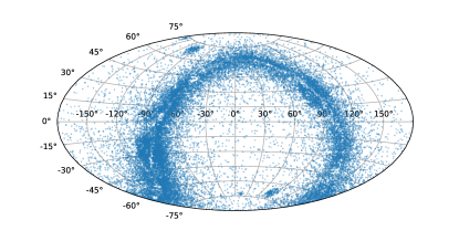
Figure 3: Aitoff projection of a random sample of $25\,000$ sources from the Gaia DR2 dataset.

Batista et al. [4] propose three input point distributions to evaluate the performance of their DT algorithm: $n$ points distributed uniformly a) in the unit cube; b) on the surface of an ellipsoid; and c) on skewed lines. Furthermore, Lee et al. [24] suggest normally distributed input points around d) the center of the unit cube; and e) several points within the unit cube – called “bubbles”. We study two variants of distribution e with the bubble centers: i) distributed uniformly at random in the unit cube; ii) along the axes of the cycle partitioner cuts – called “malicious” distribution. We furthermore test our algorithm with a real world dataset from astronomy. The Gaia DR2 catalog [13] contains celestial positions and the apparent brightness for approximately $1.7$ billion stars. Additionally, for $1.3$ billion of those stars, parallaxes and proper motions are available, enabling the computation of three-dimensional coordinates. As Figure 3 shows, the data exhibits clear structure, which can be exploited by our partitioning strategy. We use a random sample of the stars to evaluate our algorithm. All experiments are performed in three-dimensional space ($D=3$) .

Table 2 gives an overview of all input point sets, along with the size of their resulting triangulation.

The algorithm was evaluated on a machine with dual Intel Xeon E5-2683 16-core processors and 512 GiB of main memory. The machine is running Ubuntu 18.04, with GCC version 7.2 and CGAL version 4.11.

4.1 Parameter Studies

Parameter	Values
sample size $\eta(n)$	$1\text{\,}\mathrm{\char 37\relax}$, $2\text{\,}\mathrm{\char 37\relax}$, $\log n$, $\sqrt{n}$
KaHIP configuration	strong, eco, fast, parallel
edge weight $\omega(e)$	constant, inverse, log, linear
geometric primitive	bbox, exact, grid with cell sizes $c_{\mathcal{G}}=[\frac{1}{2},$1$,$2$]$
partitions $k$	$1,2,4,\dots,64$
threads $t$	$t=k$
points $n$	$[$1$,$5$,$10$,$25$,$50$]\cdot${10}^{6}$$
distribution	see Table 2

Table 3: Parameters of our algorithm (top) and the conducted experiments (bottom).

The parameters listed in Table 3 can be distinguished into configuration parameters of our algorithm and parameter choices for our experiments. In the following we examine the configuration parameters and determine robust choices for all inputs. The parameter choice influences the quality of the partitioning with respect to partition size deviation and number of points in the border triangulation. As inferior partitioning quality will result in higher execution times, we use it as indicator for our parameter tuning. Even though choices for the parameters are correlated, we present each parameter individually for clarity. We use the uniform, normal, ellipsoid and random bubble distribution for our parameter tuning and compare against the originally proposed cyclic partitioning scheme for reference.

4.2 Sample Size

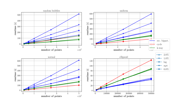
Figure 4: Sample size experiments with $k=t=16$, logarithmic edge weights, grid-based intersection test with $c_{\mathcal{G}}=1$ and parallel KaHIP.

The main goal of our divide-step is to approximate a good partitioning of the final triangulation of $DT(\mathbf{P})$. Clearly, a larger sample size $\eta(n)$ yields a better approximation at the cost of an increased runtime for the sample triangulation. On the other hand, a higher partitioning quality results in better load-balancing between partitions and smaller border triangulations. Figure 4 shows the total triangulation time for various choices of $\eta(n)$ for a fixed choice of edge weight and KaHIP configuration. The runtime of our $k$-way strategy shows little dependence on the sample size, whereas for recursive bisection the higher runtime for larger sample triangulations clearly outweighs any benefit gained from a better partitioning. We therefore choose $\eta(n)=\sqrt{n}$ as default for all subsequent experiments.

4.3 Partitioner Configuration

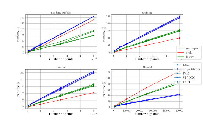
Figure 5: KaHIP configuration experiments with $k=t=16$, logarithmic edge weights, grid-based intersection test with $c_{\mathcal{G}}=1$ and $\eta(n)=\sqrt{n}$.

Numerous configuration parameters balance quality and runtime in graph partitioning [26]. KaHIP defines several presets of its parameters, each providing a good trade-off for a given runtime or quality requirement; these are, with increasing focus on runtime: strong, eco and fast [25]. Additionally, a set of parameters specifically tuned for social and web graphs is provided. The shared memory parallel version of KaHIP builds upon these configuration presets and extends them with parallel algorithms. The configuration identified as parallel in our experiments corresponds to fastsocialmultitry_parallel in [3]. In all experiments, we set the imbalance parameter for KaHIP to $\epsilon=$5\text{\,}\mathrm{\char 37\relax}$$. Figure 5 shows the total triangulation time for the various KaHIP presets for a fixed choice of edge weight and sample size. In general, the time taken by the graph partitioning algorithm is very small compared to the DT computations. Therefore, we expect the runtime to be a direct reflection of the graph partitioning quality. Our experiments confirm this notion. For instance, for the random bubble distribution the inferior partition quality of the faster eco preset compared to strong leads to an increase of triangulated points of $3.6\text{\,}\mathrm{\char 37\relax}$ at the gain of $1.5\text{\,}\mathrm{s}$ in runtime – $2.4\text{\,}\mathrm{\char 37\relax}$ of the total runtime. The parallel KaHIP configuration achieves a similar runtime as eco and only a slightly worse cut than strong ($0.5\text{\,}\mathrm{\char 37\relax}$) and will be the default for all subsequent experiments.

4.4 Edge Weights

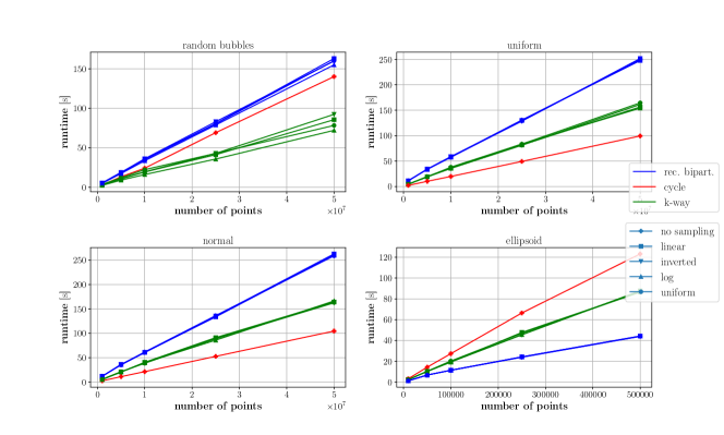
Figure 6: Edge weights experiments with $k=t=16$, parallel KaHIP, grid-based intersection test with $c_{\mathcal{G}}=1$ and $\eta(n)=\sqrt{n}$

As discussed in Section 3, sparse regions of the input points – which are desirable as partition borders – result in long Delaunay edges in the sample triangulation. Since graph partitioning minimizes the weight of the cut edges, the edge weight needs to be inversely proportional the Euclidean length of the edge, refer to Table 1. Figure 6 shows the total triangulation time for the various proposed edge weights for a fixed choice of KaHIP configuration and sample size. As dense regions of the input point set are reflected by many short edges in the sample triangulation, even constant edge weights result in a sensible partitioning. However, for input distributions with an exploitable structure, such as random bubbles, logarithmic edge weights lead to $2.3\text{\,}\mathrm{\char 37\relax}$ fewer triangulated points, due to the increased incentive to cut through long – ergo cheap – Delaunay edges.

4.5 Geometric Primitive

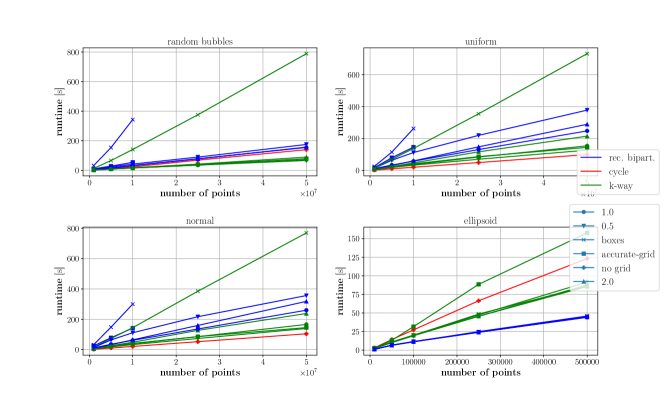
Figure 7: Intersection test experiments with $k=t=16$, logarithmic edge weights, parallel KaHIP and $\eta(n)=\sqrt{n}$.

The geometric primitive used to determine the border simplices influences both the number of simplices in the border (accuracy) and the runtime required for the primitive itself. The intersection tests introduced in Section 3.2 each provide their own trade-off between accuracy and runtime. The grid-based intersection test requires the grid cell size as further configuration parameter, which introduces a trade-off between runtime – mainly memory allocation for the grid data structure – and accuracy. Figure 7 shows the total triangulation time for the bounding box, exact and grid-based intersection test, the latter for various choices of cell size $c_{\mathcal{G}}$. The bounding box test produces very large border triangulation and suffers from the resulting runtime penalty. On the contrary, the exact test produces the smallest border triangulation, the test itself, however, is rather expensive. The grid-based test provides a good trade-off between the two strategies. The finer grid better approximates the exact test. For the uniform and normal distribution the $k$-way strategy clearly profits from the smaller border triangulation, whereas the effects for distributions with a underlying structure are less pronounced. The impact of the finer grid on the runtime becomes apparent for the recursive bisection strategy, which needs to allocate memory repeatedly. We use the grid-based intersection test with $c_{\mathcal{G}}=1$ as default for all subsequent experiments.

4.6 Partitioning Quality

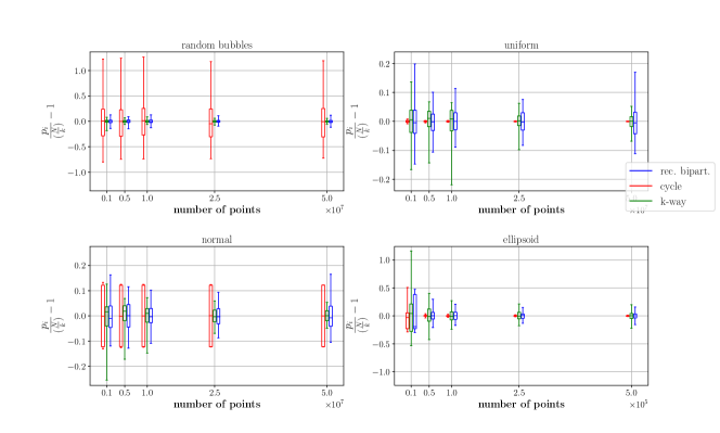
(a) sample size $\eta(n)=$0.01$n$

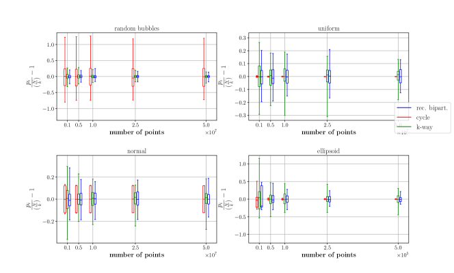
(b) sample size $\eta(n)=\sqrt{n}$

Figure 8: Deviation from the ideal partition size for $k=t=16$, parallel KaHIP, logarithmic edge weights and grid-based intersection test with $c_{\mathcal{G}}=1$.

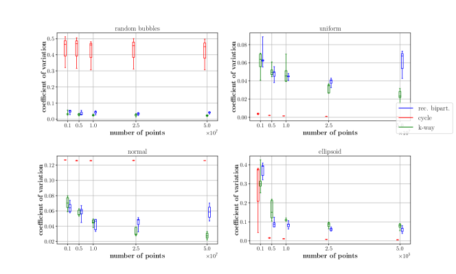
(a) sample size $\eta(n)=$0.01$n$

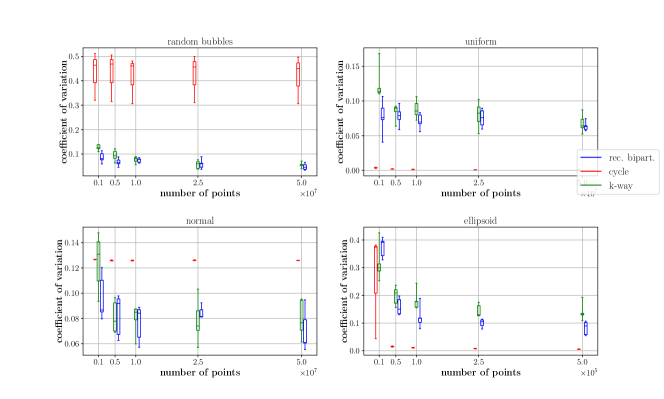
(b) sample size $\eta(n)=\sqrt{n}$

Figure 9: Coefficient of variation of the partition sizes for $k=t=16$, parallel KaHIP, logarithmic edge weights and grid-based intersection test with $c_{\mathcal{G}}=1$.

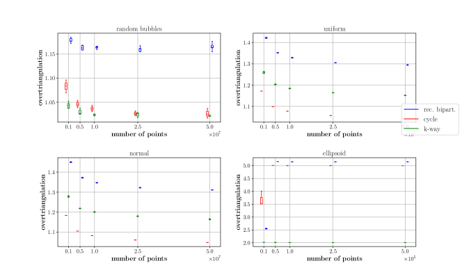
(a) sample size $\eta(n)=$0.01$n$

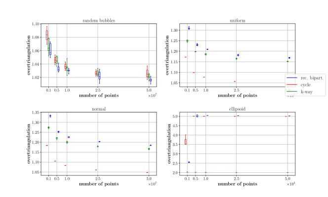
(b) sample size $\eta(n)=\sqrt{n}$

Figure 10: Overtriangulation factor for $k=t=16$, parallel KaHIP, logarithmic edge weights and grid-based intersection test with $c_{\mathcal{G}}=1$.

Given a graph partitioning $\begin{pmatrix}V_{1}&\dots&V_{k}\end{pmatrix}$, its quality is defined by the weight of its cut, $\sum_{e\in C}\omega(e)$ for $C:=\{e=(u,v),e\in E\text{ and }u\in V_{i},v\in V_{j}\text{ with }i\neq j\}$. As mentioned in Section 3, the balance of the graph partitioning is ensured by the imbalance parameter $\epsilon$, $\left|V_{i}\right|\leq(1+\epsilon)\lceil\frac{|V|}{k}\rceil$ for all $i\leq k$. When the partitioning of the sample triangulation is extended to the entire input set, this guarantee no longer holds. We therefore study two quality measures: i) the deviation from the ideal partition size and ii) the coefficient of variation of the partition sizes.

The deviation from the ideal partition size is given by $\nicefrac{{p_{i}}}{{\frac{N}{k}}}-1$, for $k$ partitions with $N$ points in total and partition sizes $p_{i}$, $i\leq k$, and is shown in Figure 8 for a fixed choice of KaHIP configuration, edge weights and two different sample sizes. Our sample-based approach produces almost equally sized partitions for the random bubble distribution and clearly outperforms the cyclic partitioning scheme. The larger sample size of $$0.01$n$ results in a more balanced partitioning compared to $\sqrt{n}$. Considering the uniform distribution, the cyclic partitioning scheme produces perfectly balanced partitions with smooth cuts between them, whereas our new divide-step suffers from the jagged border between the partitions.

The coefficient of variation $c_{v}$ of the partition sizes $p_{i}=|\mathbf{P}_{i}|$, $i\leq k$, is given by

$$c_{v}=\frac{\sigma}{\mu}=\frac{\sqrt{\frac{\sum_{i\leq k}(p_{i}-\mu)^{2}}{k-1}}}{\frac{\sum_{i\leq k}p_{i}}{k}}.$$

Figure 9 shows $c_{v}$ for a fixed choice of KaHIP configuration, edge weights and two different sample sizes. For all distributions, our sample-based partitioning scheme robustly achieves a $c_{v}$ of $\approx 6\text{\,}\mathrm{\char 37\relax}$ and $\approx 12\text{\,}\mathrm{\char 37\relax}$ for sample sizes $\sqrt{n}$ and $$0.01$n$, respectively. Both lie above the chosen imbalance of the graph partitioning of $\epsilon=$5\text{\,}\mathrm{\char 37\relax}$$, as expected. The larger sample size not only decreases the average imbalance but also its spread for various random seeds. Moreover, the deficits of the original cyclic partitioning scheme become apparent: whereas it works exceptionally well for uniformly distributed points, it produces inferior partitions in the presence of an underlying structure in the input, as found for instance in the random bubble distribution.

In total, our recursive algorithm triangulates more than the number of input points due to the triangulation of the sample points, and the triangulation(s) of the border point set(s). We quantify this in the overtriangulation factor $o_{DT}$, given by

$$o_{DT}:=\frac{|\mathbf{P}|+\sum|\mathbf{P}_{S}|+\sum|\operatorname{vertices}(\mathbf{B})|}{|\mathbf{P}|}.$$

$\mathbf{B}$ is the set of border simplices, refer to Line 15 of Algorithm 1. For direct $k$-way partitioning, only one sample and one border triangulation are necessary; for recursive bisectitioning there are a total of $k-1$ of each. Figure 10 shows the overtriangulation factor for a fixed choice of KaHIP configuration, edge weight and two different sample sizes. For all distributions, the larger sample size reduces the oversampling factor. As the partitioning of the larger sample DT more closely resembles the partitioning of the full DT, the number of points in the border triangulation is reduced. For the random bubble distribution, the overtriangulation factor is on par or below that of the original cyclic partitioning scheme. The ellipsoid distribution is specifically tailored to be a hard input. Due to its large convex hull, almost all points are part of the border triangulation, therefore the oversampling factor is bound by the maximum recursion depth. For the normally distributed input point set, the central dense region needs to be cut multiple times in order to ensure balance between the partition size. Thus, more points are part of the border point set. For the uniform distribution, our new divide-step suffers from the jagged border between the partitions compared to the smooth cut produced by the cyclic partitioning scheme. This results in more circumhyperspheres intersecting another partition and thus the inclusion of more points in the border triangulation. Our experiments with the exact intersection test primitive confirm this notion.

4.7 Runtime Evaluation

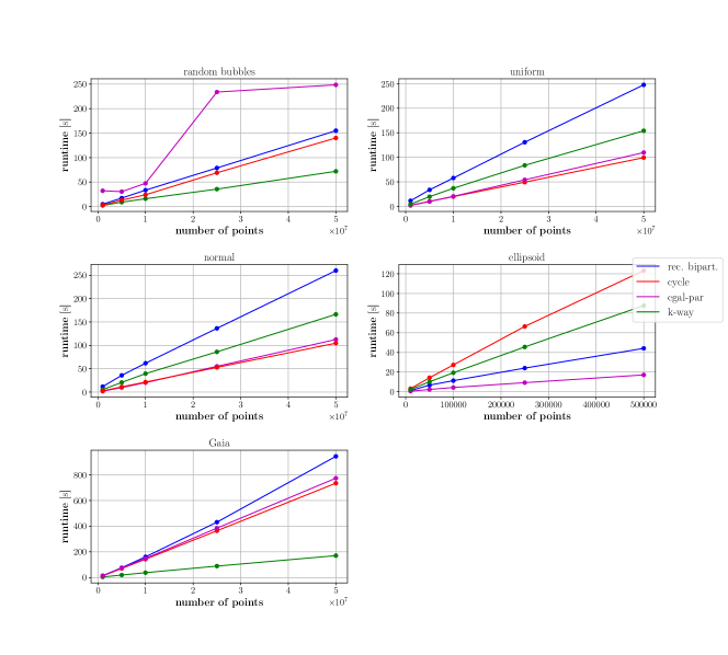
Figure 11: Runtime evaluation for $k=t=16$, parallel KaHIP, $\eta(n)=\sqrt{n}$, grid-based intersection test with $c_{\mathcal{G}}=1$ and logarithmic edge weights.

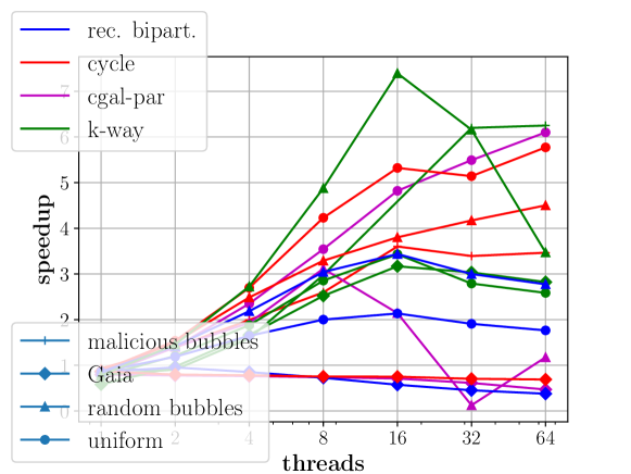
Figure 12: Absolute speedup over sequential CGAL for $k=t$, parallel KaHIP, $\eta(n)=\sqrt{n}$, grid-based intersection test with $c_{\mathcal{G}}=1$ and logarithmic edge weights. All distributions are tested with the maximum number of points given in Table 2.

We conclude our experiments with a study of the runtime of Algorithm 1 with our sample-based divide step against the originally proposed cyclic division strategy as well as the parallel incremental insertion algorithm of CGAL. Figure 11 shows the total triangulation time for a fixed choice of KaHIP configuration, edge weights and sample size.

Direct $k$-way partitioning performs best on the random bubbles distribution, with a speedup of up to $50\text{\,}\mathrm{\char 37\relax}$ over the cyclic partitioning scheme. CGAL’s parallel incremental insertion algorithm requires locking to avoid race conditions. It therefore suffers from high contention in the bubble centers, resulting in a $350\text{\,}\mathrm{\char 37\relax}$ speedup for our approach. For uniformly distributed points, our new divide-step falls behind the cyclic partitioning scheme as there is no structure to exploit in the input data and due to the higher overtriangulation factor, as discussed in the previous section. However, comparing an $o_{DT}=1.15$ for $k$-way partitioning to $o_{DT}=1.05$ for cyclic partitioning – about a $10\text{\,}\mathrm{\char 37\relax}$ increase – only explains part of the $52\text{\,}\mathrm{\char 37\relax}$ slowdown. Further investigation is therefore required to identify – and mitigate – the source of the remaining slowdown.

Of particular interest is the scaling behavior of our algorithm with an increasing number of threads. Figure 12 shows a strong scaling experiment for a fixed choice of KaHIP configuration, edge weights and sample size. The absolute speedup over the sequential CGAL algorithm is given by $\text{Speedup}(t):=\frac{T_{\text{CGAL}}}{T(t)}$ for $t$ threads.

In the presence of exploitable input structure – such as for the random bubble distribution – direct $k$-way partitioning scales well on one physical processor (up to 16 cores). It clearly outperforms the original cyclic partitioning scheme and the parallel DT algorithm of CGAL. Nevertheless, it does not scale well to two sockets ($t>16$ threads) and hyper-threading ($t>32$ threads). The overtriangulation factor of $1.19$ for 64 threads compared to $1.015$ for 16 suggests that the size of the input is not sufficient to be efficiently split into 64 partitions.

Considering our real world dataset, the direct $k$-way partitioning scheme also exhibits the best scaling behavior. As illustrated in Figure 3, the dataset comprises a large dense ring accompanied by several smaller isolated regions. This can be exploited to reduce border triangulation sizes and achieve a speedup, compared to the slowdown for the cyclic partitioning scheme and CGAL’s parallel algorithm. The former is due to large border triangulations in the central ring, whereas the latter suffers from contention in the central region.

The performance for normally distributed points can be attributed to the high overtriangulation factor, refer to Figure 10 and its discussion in the previous section.

Clearly, direct $k$-way partitioning outperforms recursive bisection in every configuration. Following the theoretical considerations in Section 3.1 regarding the number of merge-steps required, this is to be expected. A measure to level the playing field would be to only allow for $\eta(n)$ total number of sample points on all levels, i. e. adjust the sample size on each level of the recursion according the expected halving of the input size.

5 Conclusions

We present a novel divide-step for the parallel D&C DT algorithm presented in [18]. The input is partitioned according to the graph partitioning of a Delaunay triangulation of a small input point sample. The partitioning scheme robustly delivers well-balanced partitions for all tested input point distributions. For input distributions exhibiting an exploitable underlying structure, it further leads to small border triangulations and fast merging. On favorable inputs, we achieve almost a factor of two speedup over our previous partitioning scheme and over the parallel DT algorithm of CGAL. These inputs include synthetically generated data sets as well as the Gaia DR2 star catalog. For uniformly distributed input points, the more complex divide-step incurs an overall runtime penalty compared to the original approach, opening up two lanes of future work: i) smoothing the border between the partitions to reduce the overtriangulation factor, and/or ii) an adaptive strategy that chooses between the classical partitioning scheme and our new approach based on easily computed properties of the chosen sample point set, before computing its DT. Furthermore, building on the idea of Lee et al. [24], the partition borders could be traced with Delaunay edges to avoid merging all together. The sample-based divide step can also be integrated into our distributed memory algorithm presented in [18], where the improved load-balancing and border size reduces the required communication volume for favorable inputs.

References

- Aggarwal et al. [1988] A Aggarwal, B Chazelle, and L Guibas. Parallel computational geometry. Algorithmica, 3(1):293–327, 1988.
- Akhremtsev et al. [2017] Y. Akhremtsev, T. Heuer, P. Sanders, and S. Schlag. Engineering a direct k-way Hypergraph Partitioning Algorithm. In Workshop on Algorithm Engineering and Experiments, (ALENEX), pages 28–42. SIAM, 2017.
- Akhremtsev et al. [2018] Yaroslav Akhremtsev, Peter Sanders, and Christian Schulz. High-quality shared-memory graph partitioning. In Marco Aldinucci, Luca Padovani, and Massimo Torquati, editors, Euro-Par 2018: Parallel Processing, pages 659–671. Springer, 2018.
- Batista et al. [2010] Vicente H.F. Batista, David L. Millman, Sylvain Pion, and Johannes Singler. Parallel geometric algorithms for multi-core computers. Computational Geometry, 43(8):663–677, 2010.
- Bentley [1975] JL Bentley. Multidimensional binary search trees used for associative searching. Communications of the ACM, 18(9):509–517, 1975.
- Blelloch et al. [1999] E. G. Blelloch, L. G. Miller, C. J. Hardwick, and D. Talmor. Design and implementation of a practical parallel delaunay algorithm. Algorithmica, 24(3):243–269, 1999.
- Chen [2010] Min-Bin Chen. The Merge Phase of Parallel Divide-and-Conquer Scheme for 3D Delaunay Triangulation. In International Symposium on Parallel and Distributed Processing with Applications (ISPA), pages 224–230. IEEE, 2010.
- Chen and Gotsman [2012] R. Chen and C. Gotsman. Localizing the delaunay triangulation and its parallel implementation. In International Symposium on Voronoi Diagrams in Science and Engineering (ISVD), pages 24–31. IEEE, June 2012.
- Cheng et al. [2012] Siu-Wing Cheng, Tamal K Dey, and Jonathan Shewchuk. Delaunay mesh generation. CRC Press, 2012.
- Chrisochoides [2006] Nikos Chrisochoides. Parallel mesh generation. In Are Magnus Bruaset and Aslak Tveito, editors, Numerical Solution of Partial Differential Equations on Parallel Computers, pages 237–264. Springer, 2006.
- Chrisochoides and Nave [2000] Nikos Chrisochoides and Démian Nave. Simultaneous mesh generation and partitioning for delaunay meshes. Mathematics and Computers in Simulation, 54(4):321 – 339, 2000.
- Cignoni et al. [1998] P Cignoni, C Montani, and R Scopigno. DeWall: A fast divide and conquer Delaunay triangulation algorithm in . Computer-Aided Design, 30(5), 1998.
- Collaboration [2018] Gaia Collaboration. Gaia data release 2. summary of the contents and survey properties. arXiv, (abs/1804.09365), 2018.
- Delaunay [1934] B. Delaunay. Sur la sphère vide. A la mémoire de Georges Voronoï. Bulletin de l’Académie des Sciences de l’URSS. Classe des Sciences Mathématiques et Naturelles, (6):793–800, 1934.
- Devillers [2002] O. Devillers. The delaunay hierarchy. International Journal of Foundations of Computer Science, 13(02):163–180, 2002.
- Frazer and McKellar [1970] W. D. Frazer and A. C. McKellar. Samplesort: A sampling approach to minimal storage tree sorting. volume 17, pages 496–507. ACM, July 1970.
- Fuetterling et al. [2014] Valentin Fuetterling, Carsten Lojewski, and Franz-Josef Pfreundt. High-Performance Delaunay Triangulation for Many-Core Computers. In Eurographics/ ACM SIGGRAPH Symposium on High Performance Graphics. The Eurographics Association, 2014.
- Funke and Sanders [2017] D. Funke and P. Sanders. Parallel -d delaunay triangulations in shared and distributed memory. In Workshop on Algorithm Engineering and Experiments (ALENEX), pages 207–217. SIAM, 2017.
- Hert and Seel [2015] Susan Hert and Michael Seel. dD convex hulls and delaunay triangulations. In CGAL User and Reference Manual. CGAL Editorial Board, 4.7 edition, 2015.
- Karypis and Kumar [1998] G. Karypis and V. Kumar. A fast and high quality multilevel scheme for partitioning irregular graphs. SIAM Journal on Scientific Computing, 20(1):359–392, 1998.
- Kernighan and Lin [1970] B. W. Kernighan and S. Lin. An Efficient Heuristic Procedure for Partitioning Graphs. The Bell System Technical Journal, 49(2):291–307, Feb 1970.
- Kohout et al. [2005] Josef Kohout, Ivana Kolingerová, and Jiří Žára. Parallel Delaunay triangulation in E2 and E3 for computers with shared memory. Parallel Computing, 31(5):491–522, 2005.
- Larsson et al. [2007] Thomas Larsson, Tomas Akenine-Möller, and Eric Lengyel. On Faster Sphere-Box Overlap Testing. Journal of Graphics, GPU, and Game Tools, 12(1):3–8, 2007.
- Lee et al. [2001] Sangyoon Lee, Chan-Ik Park, and Chan-Mo Park. An improved parallel algorithm for delaunay triangulation on distributed memory parallel computers. Parallel Processing Letters, 11:341–352, 2001.
- Sanders and Schulz [2011] Peter Sanders and Christian Schulz. Engineering multilevel graph partitioning algorithms. In Camil Demetrescu and Magnús M. Halldórsson, editors, Algorithms – ESA 2011, pages 469–480, Berlin, Heidelberg, 2011. Springer.
- Sanders and Schulz [2013] Peter Sanders and Christian Schulz. Think Locally, Act Globally: Highly Balanced Graph Partitioning. In Proc. of Int. Symp. on Experimental Algorithms (SEA’13), volume 7933 of LNCS, pages 164–175. Springer, 2013.
- Sanders et al. [2018] Peter Sanders, Sebastian Lamm, Lorenz Hübschle-Schneider, Emanuel Schrade, and Carsten Dachsbacher. Efficient parallel random sampling – vectorized, cache-efficient, and online. ACM Trans. Math. Softw., 44(3):29:1–29:14, January 2018.
- Shewchuk [1996] JR Shewchuk. Triangle: Engineering a 2D quality mesh generator and Delaunay triangulator. Applied Computational Geometry Towards Geometric Engineering, 1148:203–222, 1996.
- Shewchuk [1997] JR Shewchuk. Adaptive Precision Floating-Point Arithmetic and Fast Robust Geometric Predicates. Discrete & Computational Geometry, 18(3):305–363, October 1997.
- Simon and Teng [1997] H. D. Simon and S.-H. Teng. How good is recursive bisection? SIAM Journal on Scientific Computing, 18(5):1436–1445, September 1997.
- Su and Drysdale [1995] Peter Su and Robert L. Scot Drysdale. A comparison of sequential delaunay triangulation algorithms. In Symposium on Computational Geometry (SCG), pages 61–70. ACM, 1995.
- van den Bergen [1997] Gino van den Bergen. Efficient collision detection of complex deformable models using aabb trees. Journal of Graphics Tools, 2(4):1–13, 1997.