Building bridges: matching density functional theory with experiment

Abstract

We will discuss the key concepts in density functional theory (DFT), how it can be used to model experimental data, and consider how the synergy between DFT and experiment can give significant insights. The discussion will centre on the scanning tunnelling microscope (STM) and surface problems, tracking the author’s personal interest, though the general principles are widely applicable.

1 Introduction

Over the last fifty years, as modern computing has emerged and scientific specialisms have increased, the traditional division of experimental and theoretical physics has gained a third category, computational physics, which has gained steadily in importance. As a discipline it bridges between theory, often too complex to admit analytic solutions, and experiment, where insight from theory is required to interpret results. The implementation of a complex theory as an efficient computer program which is capable of generating useful results is challenging; understanding the limitations of the resulting program is also key to its appropriate use.

In the realm of atomistic simulations (covering problems as diverse as physics, chemistry, materials, earth sciences and biochemistry) the most accurate results are provided using a quantum mechanical approach to modelling the interactions between atoms, but this is an archetype of a theory that cannot give analytic solutions to realistic problems. The most commonly used approach to finding practical, approximate solutions is known as density functional theory (DFT), which has become ubiquitous in many fields. It is sufficiently mature that there are various commercial packages that can be used to generate plausible output, with little understanding of the reliability of the results. Moreover, there are a number of textbooks covering the theory and application in more detail than is possible here, such as Refs. [1, 2, 3, 4].

As computers have become more powerful and approaches more efficient, the size of systems that can be addressed (in this case characterised by the number of atoms)has grown to the nanoscale. At the same time, experimental probes have become more sensitive, and can address length scales which are on the same level as modelling. Many experimental probes involve some form of averaging over a relatively large area (for instance diffraction methods), which requires a very different approach to those methods that give atomic-scale, real-space resolution. The scanning tunneling microscope (STM) gives atomic detail on metallic and semiconducting surfaces, though it involves a convolution of atomic and electronic structure which is often challenging to unravel. This is where a close collaboration between experiment and modelling is valuable: it can enable insights that the individual disciplines cannot give. However, it can take time, with both sides needing to learn the capabilities and restrictions of the other, as well as different ways of thinking and talking.

Over the course of twenty years research in this area, I have found that the combination of DFT modelling with atomic-resolution STM gives fascinating insight into a variety of systems and problems. It is not, however, a simple process to generate successful collaborations, and requires a willingness on both sides to learn the advantages and limitations of respective approaches. I will describe the basic theory behind DFT before discussing some of its limitations and the approximations that must be made to implement it successfully. I will then describe two systems where the close connection between experiment and modelling has enabled insights that go well beyond what might be found with either approach alone, or even loosely coupled. I hope that the insights found here will encourage a further engagement with the challenging but rewarding question of collaboration.

2 Density Functional Theory

The key equation in a quantum mechanical description of any system, the Schrödinger equation, is one of the simplest to write: $\hat{H}|\Psi\rangle=E|\Psi\rangle$; it is, however, impossible to solve exactly for any system more complex than a hydrogen atom. Density functional theory is one of many ways to simplify the complexity. Let us start without approximation, considering what makes up the Hamiltonian, $\hat{H}$, for a system of atoms:

$$\hat{H} = \hat{T}_{ions}+\hat{T}_{e}+\hat{V}_{II}+\hat{V}_{eI}+\hat{V}_{ee}$$

$$= -\sum_{I}\frac{\nabla^{2}_{I}}{2M_{I}}-\sum_{i}\frac{\nabla^{2}_{i}}{2}+\sum_{i,j>i}\frac{1}{\mid\mathbf{r}_{i}-\mathbf{r}_{j}\mid}+\sum_{I,J>I}\frac{Z_{I}Z_{J}}{\mid\mathbf{R}_{I}-\mathbf{R}_{J}\mid}-\sum_{I,i}\frac{Z_{I}}{\mid\mathbf{R}_{I}-\mathbf{r}_{i}\mid},$$

where $\mathbf{r}_{i}$ and $\mathbf{R}_{I}$ indicate electron and ion positions, respectively, $M_{I}$ is ionic mass and $Z_{I}$ is the charge on the ion. The terms are simply the kinetic energies of the ions and electrons (at this stage we are treating the system with a single many-body wavefunction, and both ions and electrons are quantum objects), and the electrostatic interactions between the different parts of the system. (We work in atomic units where $q_{e}=\hbar=m_{e}=4\pi\epsilon_{0}=1$.) However, as it stands, this requires a many-body wavefunction dependent on the positions of both the ions and electrons to be found.

In simplifying this problem, we can first note that the proton mass is nearly 2,000 times that of the electron, while the electrostatic forces between the particles are of similar magnitude. As a result, the change of the velocities of the nuclei on any timescale will be three orders of magnitude smaller than for the electrons. Providing that the initial velocities are not dissimilar, it is a good approximation to neglect the motion of the nuclei when considering electron motion (equivalently we can say that the electrons will be in a well-defined state—normally the ground state—when considering the nuclei). This is the Born-Oppenheimer approximation[5], which allows us to decouple the motion of the electrons and ions (further discussion of the approximation, its implications and a plausible derivation can be found in Chapter V of Ref. [6]). An associated approximation that is almost inevitably made is to treat the nuclei as classical: for most simulations this is perfectly reasonable, though the mixed classical-quantum nature of the resulting simulation raises interesting formal (or even philosophical) questions; this approximation is often known as the Ehrenfest approximation. The forces on the ions are found from a mean-field approximation, using the electronic charge density.

However, we are still left with the complex task of finding the many-body wavefunction that describes the electronic ground state of the system. There are many approaches to this problem (which, since we have removed the ionic degrees of freedom, now cannot be solved exactly for a system more complex than helium); broadly they are divided into two classes which are often described as wavefunction methods and density methods. The simplest wavefunction method is the Hartree-Fock method, which represents the many-body wavefunction as a Slater determinant of single-particle wavefunctions. However, the density methods are what will concern us here, specifically density functional theory (DFT).

A model system that is often used to gain insight into more complex electronic systems, and that forms an excellent starting point for understanding DFT, is the uniform electron gas (which is characterised by the electon density). Consider a set of electrons contained in a box, with no potential acting on them; they move freely, and the density of the gas can be taken to be the same everywhere. If we neglect the interactions between the electrons, then the only contribution to the energy is from the kinetic energy of the electrons. Whatever conditions we apply at the boundaries of the box (closed–reflecting the electrons–or periodic), the electronic states will be characterised by wavevectors, $\mathbf{k}$, which also give the kinetic energies of the states as $k^{2}/2$. The total energy is then simply the sum over the number of occupied states, or in the limit of a very large system, the integral over these states; in this case it will depend on the wavevector of the highest occupied state. It is easy to show that the number of states that are occupied, and hence the total energy of the electronic system, depends only on the electron density of the system. (In a three dimensional system, this dependency is given by $E_{\mathrm{tot}}\propto n^{{5/3}}$.)

The model as described so far is for an ideal, homogeneous system, and lacks two key ingredients necessary for modelling realistic systems: spatial variation and electron-electron interactions. Spatial inhomogeneity in the system will be provided by an external potential $V(\mathbf{r})$, typically coming from the ions. The electron density will become spatially inhomogeneous in response to the potential. The energy due to the interaction between the density and the potential is easily found (using the classical electrostatic interaction, $E_{V}=\int V(\mathbf{r})n(\mathbf{r})\mathrm{d}\mathbf{r}$). When the density is not homogeneous, the kinetic energy is more problematic, and requires some form of approximation. As early as 1927, Thomas-Fermi theory (well reviewed in Ref. [8]) suggested a way forward. The key approximation in Thomas-Fermi theory is to apply the same approach to the kinetic energy as we did to the external potential: to calculate the total kinetic energy as the spatial integral over the kinetic energy density. If the kinetic energy per electron for an electron gas of density $n(\mathbf{r})$ is $\epsilon_{\mathrm{kin}}\left[n(\mathbf{r})\right]$ then the kinetic energy density will be $n(\mathbf{r})\epsilon_{\mathrm{kin}}\left[n(\mathbf{r})\right]$, and the total kinetic energy for the inhomogeneous system can be found by integration: $E_{\mathrm{kin}}=\int\mathrm{d}\mathbf{r}n(\mathbf{r})\epsilon_{\mathrm{kin}}\left[n(\mathbf{r})\right]$. From these formulae for the energy, and a requirement that the integrated density give the correct number of electrons, we can derive a condition that links the density and the potential, and solve for the inhomogeneous density that matches the external potential.

Adding electron-electron interactions generally takes a problem from tractable to intractable; however, the key insight from Thomas-Fermi theory is that the ground state density for the interacting system can be found by solving the non-interacting system with an effective potential; the interacting system can be mapped onto a non-interacting system. To make the effective potential we add two further terms in the energy: the classical electrostatic potential due to the electrons; and the exchange interaction due to the indistinguishability of the electrons and their fermionic nature. The former takes the standard form, and is easily written in terms of the electron density. The latter can be found by analogy with the kinetic energy in the non-interacting case: we can find the exchange energy per electron for an electron gas of density $n(\mathbf{r})$, written as $\epsilon_{X}\left[n(\mathbf{r})\right]$, which is proportional to $n(\mathbf{r})^{1/3}$. We then approximate the total exchange energy by integrating over the electron gas, giving $E_{X}=\int n(\mathbf{r})\epsilon_{X}\mathrm{d}\mathbf{r}$.

As before, we find the ground state energy by seeking the density that minimises $E_{\mathrm{tot}}$, subject to the correct number of electrons. Remarkably, it can be shown that this gives the same condition that we found for the non-interacting case, but with an effective potential (made up of the sum of the external, Hartree and exchange potentials). So the ground state charge density of an interacting electron system is exactly the same as that of a non-interacting electron system with the effective potential.

We are now in a position to describe what has become known as Kohn-Sham density functional theory. The first stage involves formal proofs by Hohenberg and Kohn[9] which extend the ideas we have just explored in Thomas-Fermi theory, namely that the electron density alone is sufficient to determine the ground state properties of the system. The proofs showed that the ground state energy could be written as a functional of the density, and that the ground state energy can be found by optimising the density to give the minimum energy value of this functional. The resulting density gives the correct electron density distribution of the ground state. The energy is written as:

$$E=\int V(\mathbf{r})n(\mathbf{r})\mathrm{d}\mathbf{r}+\frac{1}{2}\int\int\mathrm{d}\mathbf{r}\mathrm{d}\mathbf{r}^{\prime}\frac{n(\mathbf{r})n(\mathbf{r}^{\prime})}{\lvert\mathbf{r}-\mathbf{r}^{\prime}\rvert}+G\left[n(\mathbf{r})\right]$$ (2)

where the three terms are the interaction with the external potential, the classical electrostatic energy of the electrons, and $G\left[n(\mathbf{r})\right]$ is a functional that we will discuss below. At this stage, no approximations have been made.

The second stage takes these concepts and turns them into a practical scheme[10]. As we saw for Thomas-Fermi theory, we will now show that within DFT the solution to the interacting electron problem with external potential $V(\mathbf{r})$ can be given by the same density as a non-interacting system with an effective potential, $V_{\mathrm{eff}}(\mathbf{r})$. However, unlike Thomas-Fermi theory, DFT does not use a functional for the kinetic energy, as this is generally a poor approximation; instead, we solve for the wavefunctions of the set of non-interacting electrons, using their kinetic energy, and building the charge density from the occupied states. We achieve this by defining the functional $G\left[n\right]$:

$$G\left[n(\mathbf{r})\right]=T_{s}\left[n(\mathbf{r})\right]+E_{XC}\left[n(\mathbf{r})\right]$$ (3)

where $T_{s}\left[n(\mathbf{r})\right]$ is the kinetic energy of the non-interacting electrons and $E_{xc}\left[n(\mathbf{r})\right]$ is the exchange and correlation energy, which we will define below. The wavefunctions $\psi_{i}$ are found by solving the Kohn-Sham (KS) equation:

$$\left[-\frac{1}{2}\nabla^{2}+V(\mathbf{r})+\int\frac{n(\mathbf{r}^{\prime})}{\lvert\mathbf{r}-\mathbf{r}^{\prime}\rvert}\mathrm{d}\mathbf{r}+V_{XC}(\mathbf{r})\right]\psi_{i}(\mathbf{r})=\epsilon_{i}\psi_{i}(\mathbf{r})$$ (4)

with $V_{XC}(\mathbf{r})=d\left(n\epsilon_{XC}[n]\right)/\mathrm{d}n(\mathbf{r})$, and setting:

$$n(\mathbf{r})=2\sum_{i=1}^{N/2}\lvert\psi_{i}(\mathbf{r})\rvert^{2}$$ (5)

for $N$ electrons, assuming no spin-polarisation in the system. As with Thomas-Fermi theory, it is important to note that this is a self-consistent process; the generation of the Kohn-Sham wavefunctions $\psi_{i}$ requires an input charge density.

The Hohenberg-Kohn-Sham theory gives a remarkably simple approach to the many-body problem, with the only remaining question being: what is the functional $E_{XC}\left[n(\mathbf{r})\right]$ ? This is a problem that cannot be solved exactly: the form is not known analytically, and study of how to approximate it is a hugely active field. Recall that the KS approach given above does not write the kinetic energy in terms of the density, but instead calculates the kinetic energy of the non-interacting electrons, meaning that the difference between the interacting and non-interacting kinetic energies in included in $E_{XC}$. As well as this contribution to the many-body energy, $E_{XC}$ also includes the exchange and correlation energies, which are purely quantum mechanical in their origin. We will discuss some of the most common functionals developed in Sec. 3.2.

3 Implementation

The transition from mathematical formalism to practical calculation involves decisions both of implementation (in the creation of the computer program) and instantiation (the selection of the actual calculation performed). These decisions will affect the accuracy of the final result, and need to be made carefully[11]. In this section, we will discuss the issues that arise in performing DFT calculations; in particular, the various approximations that are involved should become clear.

Any simulation can only ever address a finite number of atoms; for the simulation of an isolated molecule, this poses little problem, but for any other simulation, some decision about the extent of the simulation must be made. The resulting area of space is commonly known as the simulation cell. A simulation cell must be large enough to enclose the area of interest; it must be small enough that the result can be calculated in reasonable time.

The boundary conditions imposed on the simulation commonly take two forms: open (where the wavefunctions match a particular value at some distance, typically zero at infinity) and periodic (where the simulation cell is repeated infinitely, and the wavefunction at one boundary matches its value and derivative at the opposite boundary). The first of these is mainly used for molecular systems, while the second approach enables us to use the full power of Bloch’s theorem for periodic electronic systems, and is found in condensed matter calculations of all kinds. Modelling a non-periodic problem, such as a defect in the bulk of a material or a surface, with periodic boundaries requires a reworking of the system. With a defect, it must be surrounded by sufficient perfect bulk material to isolate it from the periodic images of itself; a surface is typically modelled with a slab of material surrounded by vacuum. The choice of symmetric surfaces or a bottom surface terminated in some inert way will depend on the details of the system being modelled. Choices made here will determine the reliability as well as the accuracy of the result, and the computational time required (better accuracy always involves more time).

When modelling the interaction between atoms that make up a material, we might ask whether all the electrons are needed. The understanding of bonding in chemistry suggests that only some electrons play a significant role in bonding (valence electrons) while others hardly change from their state in the isolated atom (core electrons). These core electrons are hardly involved in the interesting or important electronic structure of molecular or condensed matter systems. It seems reasonable, therefore, to develop approaches that remove or ignore the core electrons; these will have the advantage of reducing the number of electronic states that need to be found.

The pseudopotential method of condensed matter physics is a standard approach to the question of how to remove the core electrons; the nuclear potential, along with the electrostatic potential from the core electrons, are combined to form a new potential which is an approximation to the full atomic potential: a pseudopotential. This has the added advantage that the pseudopotential is softer than the atomic potential: it has lower curvature, and hence kinetic energy.

Pseudopotentials (sometimes PP) have been developed for over forty years, and have progressed from rather approximate forms to extremely sophisticated modern forms. As we are replacing one potential with another, there will always be an approximation made, and it is important to understand the quality of a pseudopotential; in particular, as the pseudopotential is generated for an isolated atom or ion, the transferability to different environments is key. The most common varieties of pseudopotentials found in modern electronic structure are: norm-conserving, or NC (where the integral of the pseudo-wavefunctions within a specified radius gives the same number of electrons as the all-electron calculations); ultrasoft, or US (where the norm conservation is relaxed, giving potentially smaller basis sets and faster calculations); and projector-augmented waves, or PAW (where the core electrons are present but frozen in all-electron states). All these forms of pseudopotential can be accurate if generated and used with care, and there have been recent efforts to test the accuracy of different libraries of pseudopotentials that are available[12].

The implementation of a quantum mechanical approach to modelling the electronic structure of materials requires the choice of a basis set to represent the wavefunctions; inevitably, the basis set will be incomplete, and the balance between convergence with respect to basis set and computational time is necessary. Electronic structure calculations most commonly use two broad classes of function: delocalised functions, exemplified by plane waves ($e^{i\mathbf{k}\cdot\mathbf{r}}$, where $\mathbf{k}$ is a wavevector); and localised functions, such as gaussian functions or atomic orbitals (or, in the case of a pseudopotential calculation, pseudo-atomic orbitals).

Plane waves are most widely used in condensed matter approaches: while they are not a well-conditioned choice for condensed phase systems, they are computationally very efficient and are well suited to periodic systems. In combination with PAWs or US pseudopotentials, they are extremely efficient and reliable. A variation of this basis set adds extra, localised basis sets (a process known as augmentation) to give the family of augmented plane waves; for bulk systems, the FLAPW method (full potential linearized augmented plane wave) is one of the most accurate reference methods available, and is used as the basis for the tests of the accuracy of pseudopotential libraries[12].

The basis size for plane waves is determined by the smallest and largest wavevectors. The smallest wavevector is set by the size of the simulation cell. The largest must be determined by the user, and is almost invariably set by reference to the equivalent kinetic energy (in atomic units, this is given by $k^{2}/2$), frequently known as the plane wave cutoff. This clarifies the use of pseudopotentials: a smoother potential means a lower plane wave cutoff. Plane waves have the convenient feature that the completeness of the basis set can be increased systematically simply by increasing the cutoff.

Localised orbitals generally conform to the spherical symmetry of the atom, and use a radial function multiplied by appropriate spherical harmonics. The radial functions vary; the two most common forms are: gaussian functions ($e^{-\alpha r^{2}}$), possibly with multiple gaussians combined into a single radial function; and the eigenstates of the isolated atom or pseudo-atom, often lightly confined. The main drawback of a localised orbital basis set is that there is no clear systematic way to increase the size of the basis; there are approaches (for instance, in quantum chemistry, the correlation consistent sets[13], and the numerical orbitals used in the AIMS code[14]) though these rely on extensive development and characterisation. Other basis sets are used in DFT, though not as extensively, for instance: a discrete grid representation coupled with finite differences for kinetic energy; and finite elements.

The computational resources required for DFT calculations depend strongly both on the approach chosen (including the basis set and the functional) and on the system being studied; the user should be concerned both with computational time, and memory. Different parts of the calculation scale differently with system size (generally characterised by the number of atoms, $N$) but there are limiting factors: ultimately the computer time will scale with the cube of the system size (or $\mathcal{O}(N^{3})$ scaling) with the memory scaling with its square. This behaviour tends to limit calculations to systems of tens or hundreds of atoms, with very few passing a thousand atoms.

The cost will also depend on the accuracy required: in periodic systems, the sampling of the Brillouin zone (which reduces with increasing system size); any numerical grid required for integration in real space; the size of the basis set chosen; and which electrons to include (as valence electrons) in the calculation. Particularly for grid and plane wave basis sets, the cost can depend strongly on the element: first row elements and first row transition metals often require a larger basis (the ion core is less screened than for other elements, giving larger kinetic energies).

3.1 Larger scale calculations

Where does the scaling of computer effort and memory with number of atoms originate ? The DFT eigenstates extend over all space (in practice, over the whole simulation cell). This spatial extension is responsible for the quadratic scaling of memory with system size, and the cubic scaling of computational effort. Large-scale calculations, and long time-scale calculations, can be performed more quickly using parallelisation: multiple processors are each assigned responsibility for different parts of the calculation. This area is typically known as high-performance computing (HPC), with facilities ranging from powerful workstations (a single machine with several tens of computational cores) to national centres with tens or hundreds of thousands of cores.

There are limitations on the efficiency of parallelisation: certain operations scale poorly with numbers of processors, while other operations require significant communication between processors. The fast Fourier transform (FFT) is used extensively in codes with plane wave basis sets; while exceptionally efficient implementations exist, at large system sizes it often presents a significant bottleneck. The largest calculation to date using standard DFT was demonstated on 100,000 atoms[15, 16], though just one self-consistency cycle was performed, and the calculation used used 400,000 processor cores; the same real-space code has demonstrated practical calculations on up to 10,000 atoms, but very few DFT calculations go beyond 1,000 atoms. Use of local basis sets can improve performance, largely because operations can be made local in space so that matrices become sparse.

For insulating and semiconducting systems, however, it can be shown that the electronic structure is localised in real-space[17] (this has been referred to as the “near-sightedness” principle[18]). Since the relevant information for any given point or atom can therefore be confined to a local volume, it should be possible to formulate DFT calculations in a linear scaling, or $\mathcal{O}(N)$, fashion. There are indeed a significant number of linear scaling methods, and several codes that implement these[19]. To date, the largest calculations have been demonstrated on over a million atoms[20, 21], though the stable, accurate implementation of these techniques is a challenge.

3.2 Density functionals

We have so far steadfastly avoided discussions of what density functionals are actually used; here we will give a brief overview of the classes of functional, and their most commonly used implementations. There are many reviews that can be read in this area, and we can only suggest a selection[22, 23, 24, 25].

The simplest approximation, suggested in the original derivation of DFT[10], is the local density approximation (LDA), where the exchange and correlation energy is written as:

$$E_{XC}\left[n\right]=\int\mathrm{d}\mathbf{r}n(\mathbf{r})\epsilon_{XC}[n(\mathbf{r})]$$ (6)

where $\epsilon_{XC}[n(\mathbf{r})]$ is the exchange and correlation energy per electron for a uniform electron gas of density $n(\mathbf{r})$. The exchange functional can be written analytically, while the correlation functional is fitted to exact results and calculations for the uniform electron gas from accurate methods such as quantum Monte Carlo[26]; a number of parameterisations exist, such as Ref. [27].

The resulting approximation is quite simple, and surprisingly effective; it is the only approximation possible that depends solely on the density (and thus is a local approximation). However, there are various failures and restrictions associated with this simplicity, discussed in the next section, which have provoked the development of functionals with more complex dependency on the density (e.g. gradients, giving semi-local functionals, etc.). The ultimate aim, the exact functional, can be proven to exist[9] but is not known exactly (moreover, it is not known as the end point of a series of approximations converging systematically[28]; while it is possible to calculate the exact answer for specific small systems, this is more expensive than solving the Schrödinger equation exactly[29]).

One of the key members of the field, John Perdew, coined the idea of a Jacob’s ladder of functionals[30], with successive rungs each more accurate. The increase in accuracy proceeds in stages, each of which typically increases the computational cost:

1. The local density approximation (LDA), depending only on the value of the density at each point in space, $n(\mathbf{r})$

2. Generalised gradient approximations (GGA), where the functional also depends on the magnitude of the gradient of the density, $\left|\nabla n(\mathbf{r})\right|$

3. Meta-GGA functionals include the kinetic energy density:

   $$\tau_{\sigma}(\mathbf{r})=\frac{1}{2}\sum_{i}\left|\nabla\psi_{i}(\mathbf{r}\right|^{2}$$ (7)

   where the sum is over occupied Kohn-Sham eigenstates, $\psi_{i}$, only

4. Hybrid functionals add some fraction of the exact exchange energy written in terms of the Kohn-Sham orbitals. There are some variants of hybrid functionals that introduce range-separation, where the exchange energy is calculated partly from the exact exchange and partly from GGA exchange (typically this is for solids, where the computationally expensive exact exchange is only used for short-ranged interactions)

5. The final set of functionals introduce a dependency on both unoccupied and occupied orbitals, using approaches such as the random phase approximation (RPA), but these are extremely expensive

There are other additions (notably the van der Waals density functionals discussed below) but these are the key rungs on the notional ladder of accuracy. The functional chosen depends on the type of calculation being performed. Most solid state calculations use a GGA functional (in part because most use plane waves as a basis set, and this makes hybrid calculations very expensive) though Meta-GGA is becoming more common. Many quantum chemistry calculations use a hybrid functional. Some of the most commonly used functionals include: the GGA functional PBE[31] and its variants; the hybrid functionals B3LYP[32] and PBE0[33]; the screened hybrid HSE[34]; and the meta-GGA functionals TPSS[35] and SCAN[36]. The selection and reliability of a functional depends both on the system being studied and, to some extent, the philosophy of the user. Approaches to functional creation include on the one hand ensuring that the functional conforms to known constraints and behaviours, and on the other hand fitting parameters in the functional to databases of accurate existing results. These topics are discussed further elsewhere[37, 38, 24].

4 Capabilities and Restrictions

We will briefly discuss some of the successes and limitations of DFT in general, and specific functionals in this section. There are many reviews of this area[22, 37, 39, 40, 23, 38] to which the interested reader is directed.

Geometries are almost always better with GGA than LDA, which overbinds (in the solid state, lattice constants are often around 1% too small). The PBE functional[31] which is commonly used for GGA calculations overestimates lattice constants by about the same amount; the PBEsol functional[41] is a recalibration of the PBE functional for solids (losing some accuracy for atomization and total energies).

While electronic structure is often well described, the most well-known issue with LDA and GGA is that band gaps are seriously underestimated. The major contribution to this issue is the self-interaction: the expression for the electrostatic energy of the electrons includes the interaction of each electron with itself. Attempts have been made to create approaches within DFT that correct for this[42, 43] but are often hard to converge and do not improve accuracy significantly. Hybrid calculations, where some exact exchange is included, correct this issue while also improving thermochemistry, at significantly higher computational cost.

The area where much recent work has been directed is that of non-bonding interactions, specifically van der Waals forces. Significant progress has been made with semi-empirical methods that add extra forcefield terms to add dispersion[44, 45]. However, significant advances have been made in developing a fully non-local DFT dispersion functional[46], which has been extensively tested and further developed[47, 48]. There now exist excellent DFT approaches to dispersion forces.

The question of excited states is one we have not yet addressed. The DFT eigenvalues do not have any formal link to measured energy levels (beyond the frontier orbitals) but are often used as an ansatz for them. DFT is a ground state theory: the original theorems only apply to the ground state density, and hence the occupied levels. The most commonly used approach to calculated excited state energies is time-dependent DFT (TDDFT)[49, 50], while many-body perturbative methods[51][52] often build on DFT eigenvalues as their starting point. With these methods a wide variety of spectroscopies can be modelled and probed.

5 Examples of collaboration

While DFT is a powerful method for understanding the properties of molecules and materials, it is much more powerful when work is carried out in close collaboration with experiment. It is relatively easy as a DFT practitioner to create a new structure, phase or material, and to publish the result. It is more informative to select the system or structure on the basis of experimental evidence, narrowing the space of problems, and to provide insight into experimental results that go beyond the resolution or capabilities of experiment.

It is far better, though often challenging, to work in collaboration with experimental groups, with frequent feedback and discussion, giving rise to combined results that exceed what would have been possible for either discipline in isolation. The challenge in this mode of working comes from the investment required to learn about the strengths and limitations of the different techniques, and to understand how the data and insight from one can illuminate and open up the other.

This section concentrates almost exclusively on STM, as this is the technique with which I have mainly engaged. However, of course, there are many experimental techniques that can be addressed with DFT, including: NMR; TEM, especially EELS; photo-emission spectroscopy; inelastic neutron and x-ray scattering; and both IR and Raman spectroscopy, to name some of the most common.

5.1 Bismuth on Si(001)

Nanowires have been a topic of intense research recently[53], and self-assembled nanowires are very attractive from a manufacturing point of view. The structure of the nanowires (or nanolines) that self-assemble on the Si(001) surface following adsorption and annealing of bismuth required considerable time, and a concerted collaboration between experiment and theory, to unravel.

Bismuth is used in semiconductor growth as a surfactant: a material that passivates the surface, leading to flatter, smoother growth[54]. However, it was found experimentally that it has another property on silicon surfaces: it can form atomically perfect nanolines, 1 nm wide and up to microns long[55, 56, 57, 58], as shown in Figure 1. (We refer to these structures as nanolines rather than nanowires as their gap is larger than that of the surrounding surface.) The initial STM images were taken at elevated temperature, and gave little detail: the basic appearance of a nanoline with two parallel tracks was clear, but the actual width and registry with the substrate was not visible. The initial structures proposed matched these basic facts, but could not explain the key feature of these lines: their extraordinary straightness and perfection. A kink has never been observed in any bismuth nanoline, while defects are very unusual.

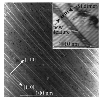
Figure 1: STM image of Bi nanolines in Si(001), taken at +2V. The inset shows a detailed scan of the nanolines, with postulated positions of silicon and bismuth dimers (subsequently shown to be in different locations). Reprinted figure with permission from Ref. [57]. Copyright 1999 by the American Physical Society.

The Si(001) surface consists of rows of dimers (pairs of Si atoms bonded together in a surface reconstruction). The model initially proposed for the Bi nanolines[57] used the available evidence, and assumed that two bismuth dimers would replace three silicon dimers, with a vacancy between them. This early model matched the basic observations , and was stable, but had one main problem: there was no mechanism to explain the straightness of the lines. At this stage, the modelling contribution was limited by the available experimental data—the energetics could be calculated, but without more detail on the structure little could be done.

These original experiments were performed at elevated temperatures to keep the surface clean, reducing the resolution of the imaging. Passivating the surrounding surface with hydrogen[59, 60] revealed that the bismuth lines in fact replaced four silicon dimers, not three, and were situated between the underlying surface dimers. The first model proposed to occupy the space of four dimers[59] suggested two vacancies bracketing a central pair of bismuth dimers, which failed to match the experimentally observed spacing and location of the parallel tracks.

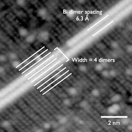
Figure 2: Bi nanolines with passivated Si(001) background, imaged in STM at -2.5V and room temperature. Substrate dimers are shown with a set of white lines, which enables registry of Bi nanolines with the substrate to be seen eaily. Reprinted from Ref. [53] by permission from Springer, copyright 2006.

The situation at this point neatly encapsulates one of the major problems for surface science, and condensed matter more generally: there is limited experimental information on a surface reconstruction or crystal structure, and a wide parameter space that could be searched with modelling. In recent years, approaches have been developed to search a wide variety of structures[61] (these methods include high throughput techniques such as the materials genome[62] and random structure searching[63], and evolving approaches such as genetic algorithms[61]) but there is little success with or application to surfaces.

We proceeded to use a combination of intuition and modelling constrained by the known properties of the system. The information available was as follows:

• The lines only formed near the Bi desorption temperature, after annealing

• The lines persisted after desorption of the remaining surface Bi

• No kink was observed in the lines, and almost no defects

• The silicon around the lines was defect-free: the lines appeared to exclude defects

• The lines replace four silicon surface dimers

• The spacing between features in the line was less than the spacing between dimers in the surface

Based on these observations, we sought structures that would be more stable than the simple $\left(2\times n\right)$ reconstruction of Bi dimers adsorbed on the surface. We used a linear-scaling tight binding code to explore the stability of possible structures[64]; the results were approximate but very fast, and enabled large scale calculations (1,000+ atoms) on very modest computational resources (a laptop in the lab), as well as making the rapid testing of many candidate structures almost trivial. Promising candidate structures were refined using DFT; these calculations showed that the tight-binding results were, with one unimportant exception, correct in the ordering of stability of structures.

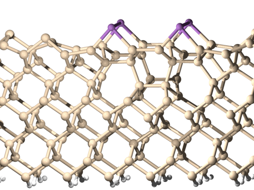
Figure 3: The Haiku model for the Bi nanolines[65], seen in perspective. This slab model has ten layers of silicon, with the base fixed and terminated in hydrogen to mimic semi-infinite bulk. The normal tetrahedral bonding of silicon is clear in the lower layers. The significant reconstruction below the bismuth dimers, shown in purple, is formed of five-membered and seven-membered rings. The Bi nanoline replaces four silicon dimers in the surface.

The structure that was identified as the Bi nanoline[65] is shown in Fig. 3. It drew inspiration from STM observations of step edges on As-covered Ge(001) surfaces[66]. The model is named Haiku and shows considerable sub-surface reconstruction (with five-membered and seven-membered rings prominent—reminiscent of defects in carbon nanotubes). It fits all the criteria identified for the nanolines.

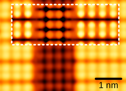
Figure 4: Main image: STM image at -2.5V of Si(001) surface after Bi nanoline growth and dosing with hydrogen. The bare haiku trench runs vertically through the figure. Inset (within dashed rectangle): Simulated STM image from DFT. Reprinted figure with permission from Ref. [67]. Copyright 2011 by the American Physical Society.

The ultimate confirmation of the correctness of the structure came when it was discovered that a high flux of atomic hydrogen could remove the Bi[68]. An STM image of the resulting structure is shown in Fig. 4; there is a clear difference between the surface and the area left vacant by Bi. Inset into the image is a simulated STM image from DFT of the Haiku structure with Bi replaced by hydrogen atoms; the agreement is remarkable.

Further exploration of the Bi lines has found other detailed features that required more careful collaboration between experiment and theory: a peculiar feature observed in STM with sub-Ångström dimensions was shown to be a Si dimer substituting for a Bi dimer in the line, rapidly flipping between different orientations[69]; and subtle changes in the appearance of the nanoline with STM voltage was shown to result from electronic coupling between the background silicon and the Bi dimers[70]. In all cases the information available from either experiment or theory was incomplete, and the final interpretation was only possible with careful dialogue and exploration between the two.

5.2 TiSe₂

TiSe₂ is a quasi-two-dimensional material, one of the large family of transition metal dichalcogenides, consisting of a sandwich of a hexagonal layer of Ti between two hexagonal layers of Se, with successive sandwiches loosely bound together by van der Waals forces; this is schematically illustrated in the left-hand side of Fig. 5. The material develops a charge-density wave (CDW) below $\sim$200K, which is commensurate with the lattice (somewhat unusually for this class of material). It is not clear whether it is a semiconductor with a very small indirect gap or a semimetal[71, 72]. It can be made superconducting by application of pressure[73] or doping with Cu[74]. These properties make it a very interesting system to study, particularly as it gives considerable opportunity to gain insight into the relationship between the formation and development of the CDW and superconductivity. Using STM and DFT modelling together gives the opportunity to study the correlation between the CDW and the material’s electronic structure in real space.

As with all materials, there are defects in the TiSe₂ samples that are grown. Understanding the real-space location of these native defects in TiSe₂ in both the non-CDW and CDW forms will give important points of reference when studying more complex features in the system. Similarly, understanding the defects without the CDW is an important precursor to understanding the effect of the CDW on the defects, and vice versa. The information available from STM alone is not enough to identify defects; using the appearance of the defects and how they change with imaging bias, alongside DFT modelling of likely defect sources, is the only way to characterise the defects.

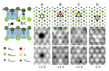
Figure 5: Top left: schematic illustration of the structure of TiSe₂ and the location of the four defects. Main: schematic, STM and DFT images of four defects in TiSe₂, without charge density wave. Reprinted figure with permission from Ref. [75]. Copyright 2014 by the American Physical Society.

The right hand side of Fig. 5 (columns A-D) shows the four native defects identified from TiSe₂ samples grown with iodine-vapour transport. The middle row shows atomic resolution STM images of the four defects identified in the samples; most (A-C) were clearest in empty states, or positive sample bias, while one (D) was only seen in filled states, or negative samle bias. From these images, and the likely contaminants or lattice defects, a list of DFT simulations was created. For each of these, after structural relaxation, STM images were simulated at a variety of voltages. The bottom row in Fig. 5 shows the best match for each STM image, while the top row shows a schematic of the proposed defect. Iodine (B) is present because of the growth process, while oxygen (C) is almost unavoidable; the top layer vacancy (A) is likely to come from desorption of Se or I/O substitutional defects following cleaving of the crystal. Ti intercalates (inserts into the van der Waals gaps between layers) during the growth process. The temperature of the growth process controls to some extent the excess levels of Ti incorporated in the crystal, and the defect D is only seen in crystals with Ti self-doping, which coupled with good STM agreement, suggests that this defect is a Ti intercalate. These atomically precise identifications allow future studies to identify the registry of STM images and the underlying substrate.

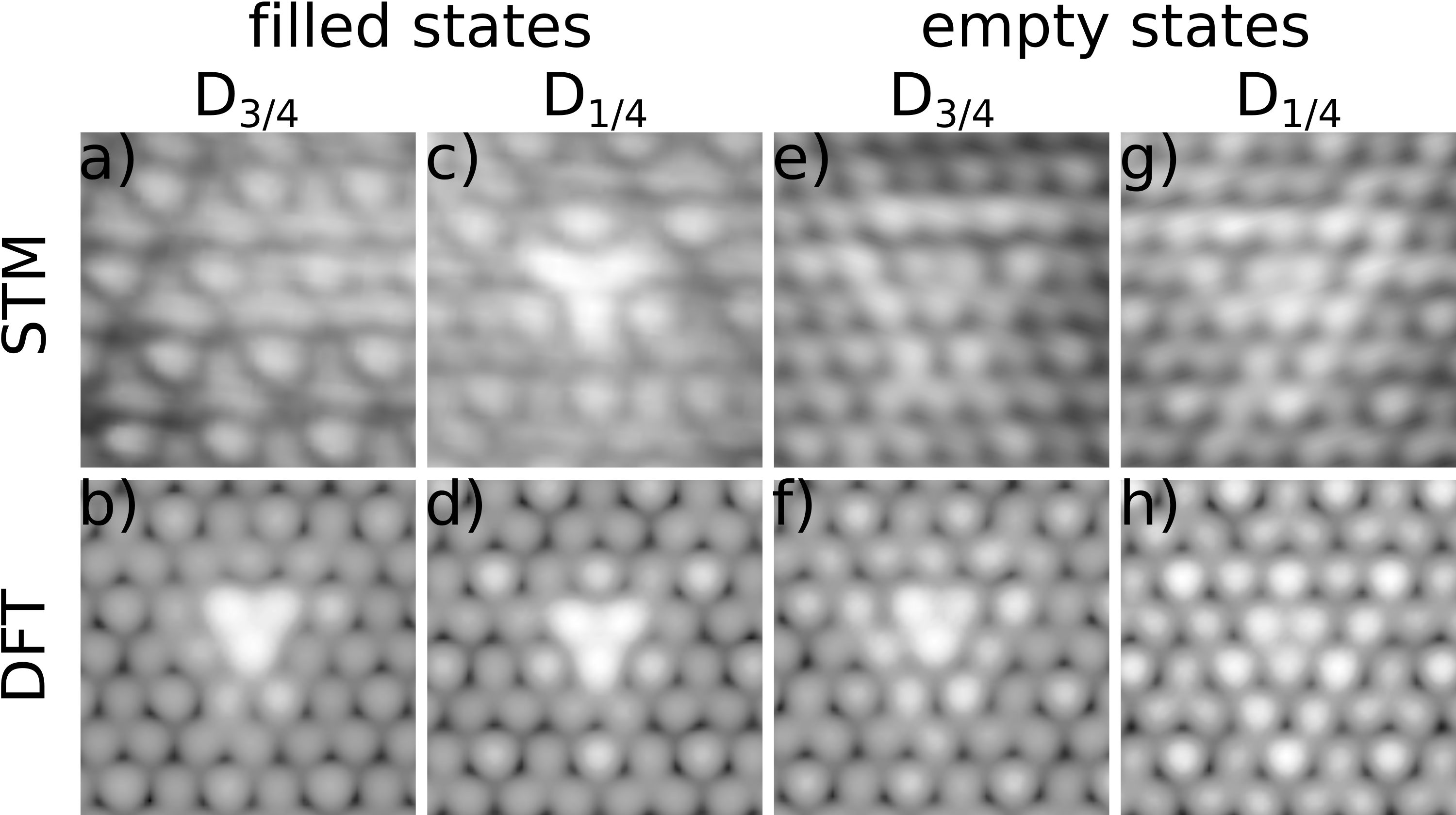
Figure 6: STM (top) and DFT simulated images (bottom) of Ti intercalate defects (type D in Fig. 5) in the presence of the CDW. Filled states bias was -150mV, empty states +150mV. Reprinted figure with permission from Ref. [76]. Copyright 2015 by the American Physical Society.

Cooling below $\sim$202K induces the formation of the charge density wave in TiSe₂, which is only visible in STM at biases below $\sim$0.2V. It takes the form of a $(2\times 2)$ periodic distortion, commensurate with the underlying lattice, with four atoms in the surface unit cell. The unit cell divides into one bright atom and three darker atoms, giving two sites for the defects, labelled 1/4 and 3/4, depending on their relation to the surface atoms. The first three defects identified in Fig. 5 above, A–C, are only slightly perturbed by the presence of the CDW, and can be well described in DFT without the CDW distortion[76]. The Ti intercalate, shown in Fig. 6, interacts more strongly with the CDW in terms of its appearance. However, despite the doping nature of this defect, it does not disrupt the CDW locally—an important observation in the light of resistivity measurements that show the macroscopic phase transition signature disappearing with Ti self-doping[77]. Overall, these measurements and modelling enabled us to rule out the formation of an incommensurate CDW, and any local change of crystal structure (for instance change from 1T to 2H polytype), and to note that there are different electronic signatures from the defects on inequivalent lattice sites.

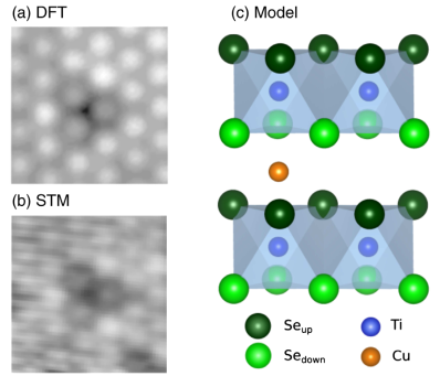
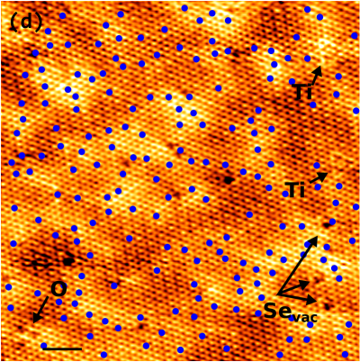
Figure 7: (a) DFT simulation and (b) STM image of an intercalated Cu atom (1.72$\times$1.72 nm², V_bias=-1.2 V, I = 30 pA). (c) Model of the 1T-Cu_xTiSe₂ showing the Cu atom position in the vdW gap. (d) Low bias image of surface showing the CDW modulation, with Cu intercalates indicated with blue dots (identified by imaging at different bias). Reprinted figure with permission from Ref. [78]. Copyright 2017 by the American Physical Society.

The ability to interrogate, in real-space, the effect of different defects and dopants on the CDW is extremely valuable, and gives new insights into the stability and formation of the CDW, as well as the relation to superconductivity. Addition of Cu, beyond a fractional doping of 0.04, induces superconductivity in 1T-TiSe₂, with a maximum $T_{C}$ of 4.1K when $x\simeq 0.08$[74], with transport measurements showing that the CDW is suppressed as the Cu fraction is increased. However, the location of the Cu atoms and their electronic signature were not known.

Using DFT, we were able to predict a likely bias voltage and appearance for the Cu intercalates, shown in Fig. 7(a) with a structural model in (c). Subsequent STM measurements found this exact appearance, as seen in Fig. 7(b)[78]. We have already established that the CDW maxima are located on Se atoms using native defects; we can now image both the Cu atom location (at relatively high bias, $\sim-1.2V$) and the local effect on the CDW (at low bias), as shown in Fig. 7(d). In particular, the CDW breaks up into nanometre-scale domains with short-range order, and other areas where the CDW amplitude is reduced. STM shows that areas with high Cu concentration correlate with the reduction of the CDW amplitude–an insight that would impossible without detailed knowledge of the location of the Cu atoms, which in turn was found only by close collaboration between experiment and modelling.

6 Conclusions

Density functional theory has become ubiquituous in many fields, but is a sufficiently complex technique that some understanding of its basic implementation in modelling packages is vital to successful use. Moreover, modelling on its own is futile, and requires at the very least comparison to experiment, while collaboration is far more rewarding.

I have given a basic outline of the theory behind DFT, as well as discussing some of the issues involved in its implementation. This should highlight the dangers of using it as a black box: many pitfalls lie in wait for the unwary user!

By focussing on two key areas of where I have had extensive collaboration with experimental groups, I have highlighted the gains that can come from spending significant time to learn the capabilities and restrictions of different methods. Understanding what can and cannot be done both with an experimental approach and with modelling is highly instructive. I hope to inspire further deep collaborations.

Abbreviations

A list of abbreviations commonly used in the field, in alphabetical order.

BLYP	Becke (exchange) and Lee, Yang & Parr (correlation) GGA functional
DFT	Density functional theory
FLAPW	Full-potential linearized augmented PW
GGA	Generalised gradient approximation
KS	Kohn-Sham
LDA	Local density approximation
LMTO	Linear muffin-tin orbital
PAW	Projector-augmented waves
PBE	Perdew, Burke & Ernzerhof GGA functional
PW	Plane wave
TDDFT	Time-dependent DFT
vdW	van der Walls (also called dispersion)
XC	Exchange and correlation

References

- [1] Parr RG, Weitao Y. Density-Functional Theory of Atoms and Molecules. Oxford University Press; 1994.
- [2] Martin RM. Electronic Structure: Basic Theory and Practical Methods. Cambridge University Press; 2004.
- [3] Giustino F. Materials Modelling using Density Functional Theory. Oxford University Press; 2014.
- [4] Kaxiras E. Atomic and electronic structure of solids. Cambridge University Press; 2003.
- [5] Born M, Oppenheimer R. Zur Quantentheorie der Molekeln. Ann Phys. 1927;84:457.
- [6] Ziman JM. Electrons and phonons. Oxford University Press; 2001. Oxford Classics Series.
- [7] Horsfield AP, Bowler DR, Ness H, et al. The transfer of energy between electrons and ions in solids. Rep Prog Phys. 2006;69(4):1195–1234. Available from: http://stacks.iop.org/0034-4885/69/1195.
- [8] Spruch L. Pedagogic notes on Thomas-Fermi theory (and on some improvements): atoms, stars, and the stability of bulk matter. Rev Mod Phys. 1991 Jan;63:151–209. Available from: https://link.aps.org/doi/10.1103/RevModPhys.63.151.
- [9] Hohenberg P, Kohn W. Inhomogeneous electron gas. Phys Rev. 1964 Nov;136:B864–B871. Available from: https://link.aps.org/doi/10.1103/PhysRev.136.B864.
- [10] Kohn W, Sham LJ. Self-Consistent Equations Including Exchange and Correlation Effects. Phys Rev. 1965;140(4A):A1133–A1138.
- [11] Bràzdovà V, Bowler DR. Atomistic Computer Simulations: A Practical Guide. WILEY-VCH Verlag Berlin GmbH; 2013.
- [12] Lejaeghere K, Bihlmayer G, Bjorkman T, et al. Reproducibility in density functional theory calculations of solids. Science (80- ). 2016 mar;351(6280):aad3000–aad3000. Available from: http://science.sciencemag.org/content/351/6280/aad3000.abstract.
- [13] Dunning TH. Gaussian basis sets for use in correlated molecular calculations. I. The atoms boron through neon and hydrogen. The Journal of Chemical Physics. 1989;90(2):1007–1023. Available from: http://dx.doi.org/10.1063/1.456153.
- [14] Blum V, Gehrke R, Hanke F, et al. Ab initio molecular simulations with numeric atom-centered orbitals. Computer Physics Communications. 2009;180(11):2175 – 2196. Available from: http://www.sciencedirect.com/science/article/pii/S0010465509002033.
- [15] Hasegawa Y, Iwata JI, Tsuji M, et al. First-principles Calculations of Electron States of a Silicon Nanowire with 100,000 Atoms on the K Computer. In: Proceedings of 2011 International Conference for High Performance Computing, Networking, Storage and Analysis; New York, NY, USA. ACM; 2011. p. 1:1–1:11; SC ’11. Available from: http://doi.acm.org/10.1145/2063384.2063386.
- [16] Hasegawa Y, Iwata JI, Tsuji M, et al. Performance evaluation of ultra-large-scale first-principles electronic structure calculation code on the K computer. The International Journal of High Performance Computing Applications. 2014;28(3):335–355. Available from: https://doi.org/10.1177/1094342013508163.
- [17] He L, Vanderbilt D. Exponential Decay Properties of Wannier Functions and Related Quantities. Phys Rev Lett. 2001 Jun;86(23):5341–5344.
- [18] Kohn W. Density functional and density matrix method scaling linearly with the number of atoms. Phys Rev Lett. 1996 Apr;76(17):3168–3171.
- [19] Bowler DR, Miyazaki T. {mathcal{O}(N)} methods in electronic structure calculations. Rep Prog Phys. 2012;75(3):36503. Available from: http://dx.doi.org/10.1088/0034-4885/75/3/036503.
- [20] Arita M, Arapan S, Bowler DR, et al. Large-scale DFT simulations with a linear-scaling DFT code CONQUEST on K-computer. J Adv Simul Sci Eng. 2014 oct;1(1):87–97. Available from: https://www.jstage.jst.go.jp/article/jasse/1/1/1_87/_article.
- [21] Bowler DR, Miyazaki T. Calculations on millions of atoms with density functional theory: linear scaling shows its potential. J Phys Condens Matter. 2010;22:74207. Available from: http://stacks.iop.org/JPhysCM/22/074207.
- [22] Becke AD. Perspective: Fifty years of density-functional theory in chemical physics. The Journal of Chemical Physics. 2014;140(18):18A301. Available from: https://doi.org/10.1063/1.4869598.
- [23] Cohen AJ, Mori-Sánchez P, Yang W. Challenges for Density Functional Theory. Chemical Reviews. 2012 01;112(1):289–320. Available from: https://doi.org/10.1021/cr200107z.
- [24] Yu HS, Li SL, Truhlar DG. Perspective: Kohn-Sham density functional theory descending a staircase. The Journal of Chemical Physics. 2016;145(13):130901. Available from: https://doi.org/10.1063/1.4963168.
- [25] Mardirossian N, Head-Gordon M. Thirty years of density functional theory in computational chemistry: an overview and extensive assessment of 200 density functionals. Molecular Physics. 2017;115(19):2315–2372. Available from: https://doi.org/10.1080/00268976.2017.1333644.
- [26] Ceperley DM, Alder BJ. Ground State of the Electron Gas by a Stochastic Method. Phys Rev Lett. 1980 Aug;45:566–569. Available from: https://link.aps.org/doi/10.1103/PhysRevLett.45.566.
- [27] Perdew JP, Wang Y. Accurate and simple analytic representation of the electron-gas correlation energy. Phys Rev B. 1992 Jun;45:13244–13249. Available from: https://link.aps.org/doi/10.1103/PhysRevB.45.13244.
- [28] Perdew JP, Ruzsinszky A, Tao J, et al. Prescription for the design and selection of density functional approximations: More constraint satisfaction with fewer fits. The Journal of Chemical Physics. 2005;123(6):062201. Available from: https://doi.org/10.1063/1.1904565.
- [29] Stoudenmire EM, Wagner LO, White SR, et al. One-dimensional continuum electronic structure with the density-matrix renormalization group and its implications for density-functional theory. Phys Rev Lett. 2012 Aug;109:056402. Available from: https://link.aps.org/doi/10.1103/PhysRevLett.109.056402.
- [30] Perdew JP, Schmidt K. Jacob’s ladder of density functional approximations for the exchange-correlation energy. AIP Conference Proceedings. 2001;577(1):1–20. Available from: https://aip.scitation.org/doi/abs/10.1063/1.1390175.
- [31] Perdew J, Burke K, Ernzerhof M. Generalized Gradient Approximation Made Simple. Phys Rev Lett. 1996;77(18):3865–3868. Available from: https://journals.aps.org/prl/abstract/10.1103/PhysRevLett.77.3865.
- [32] Becke AD. Density‐functional thermochemistry. III. The role of exact exchange. The Journal of Chemical Physics. 1993;98(7):5648–5652. Available from: https://doi.org/10.1063/1.464913.
- [33] Perdew JP, Ernzerhof M, Burke K. Rationale for mixing exact exchange with density functional approximations. The Journal of Chemical Physics. 1996;105(22):9982–9985. Available from: https://doi.org/10.1063/1.472933.
- [34] Heyd J, Scuseria GE, Ernzerhof M. Hybrid functionals based on a screened Coulomb potential. The Journal of Chemical Physics. 2003;118(18):8207–8215. Available from: https://doi.org/10.1063/1.1564060.
- [35] Tao J, Perdew JP, Staroverov VN, et al. Climbing the density functional ladder: Nonempirical meta–generalized gradient approximation designed for molecules and solids. Phys Rev Lett. 2003 Sep;91:146401. Available from: https://link.aps.org/doi/10.1103/PhysRevLett.91.146401.
- [36] Sun J, Ruzsinszky A, Perdew JP. Strongly constrained and appropriately normed semilocal density functional. Phys Rev Lett. 2015 Jul;115:036402. Available from: https://link.aps.org/doi/10.1103/PhysRevLett.115.036402.
- [37] Burke K. Perspective on density functional theory. The Journal of Chemical Physics. 2012;136(15):150901. Available from: https://doi.org/10.1063/1.4704546.
- [38] Pribram-Jones A, Gross DA, Burke K. DFT: A Theory Full of Holes? Annual Review of Physical Chemistry. 2015;66(1):283–304. PMID: 25830374; Available from: https://doi.org/10.1146/annurev-physchem-040214-121420.
- [39] Hasnip PJ, Refson K, Probert MIJ, et al. Density functional theory in the solid state. Phil Trans R Soc A. 2014;372:20130270.
- [40] Jones RO. Density functional theory: Its origins, rise to prominence, and future. Rev Mod Phys. 2015 Aug;87:897–923. Available from: https://link.aps.org/doi/10.1103/RevModPhys.87.897.
- [41] Perdew JP, Ruzsinszky A, Csonka GI, et al. Restoring the density-gradient expansion for exchange in solids and surfaces. Phys Rev Lett. 2008 Apr;100:136406. Available from: https://link.aps.org/doi/10.1103/PhysRevLett.100.136406.
- [42] Perdew JP, Zunger A. Self-interaction correction to density-functional approximations for many-electron systems. Phys Rev B. 1981 May;23:5048–5079. Available from: https://link.aps.org/doi/10.1103/PhysRevB.23.5048.
- [43] Goedecker S, Umrigar CJ. Critical assessment of the self-interaction-corrected–local-density-functional method and its algorithmic implementation. Phys Rev A. 1997 Mar;55:1765–1771. Available from: https://link.aps.org/doi/10.1103/PhysRevA.55.1765.
- [44] Grimme S, Antony J, Ehrlich S, et al. A consistent and accurate ab initio parametrization of density functional dispersion correction (DFT-D) for the 94 elements H-Pu. The Journal of Chemical Physics. 2010;132(15):154104. Available from: https://doi.org/10.1063/1.3382344.
- [45] Tkatchenko A, Scheffler M. Accurate Molecular Van Der Waals Interactions from Ground-State Electron Density and Free-Atom Reference Data. Phys Rev Lett. 2009 Feb;102:073005. Available from: https://link.aps.org/doi/10.1103/PhysRevLett.102.073005.
- [46] Dion M, Rydberg H, Schröder E, et al. Van der Waals Density Functional for General Geometries. Phys Rev Lett. 2004 Jun;92:246401. Available from: https://link.aps.org/doi/10.1103/PhysRevLett.92.246401.
- [47] Klimeš J, Michaelides A. Perspective: Advances and challenges in treating van der Waals dispersion forces in density functional theory. The Journal of Chemical Physics. 2012;137(12):120901. Available from: https://doi.org/10.1063/1.4754130.
- [48] Berland K, Cooper VR, Lee K, et al. van der Waals forces in density functional theory: a review of the vdW-DF method. Reports on Progress in Physics. 2015;78(6):066501. Available from: http://stacks.iop.org/0034-4885/78/i=6/a=066501.
- [49] Marques M, Gross E. Time-dependent density functional theory. Annual Review of Physical Chemistry. 2004;55(1):427–455. PMID: 15117259; Available from: https://doi.org/10.1146/annurev.physchem.55.091602.094449.
- [50] Marques MAL, Ullrich CA, Nogueira F, et al., editors. Time-dependent density functional theory. (Lecture Notes in Physics; Vol. 706). Springer Berlin Heidelberg; 2006.
- [51] Onida G, Reining L, Rubio A. Electronic excitations: density-functional versus many-body Green’s-function approaches. Rev Mod Phys. 2002 Jun;74:601–659. Available from: https://link.aps.org/doi/10.1103/RevModPhys.74.601.
- [52] Reining L. The GW approximation: content, successes and limitations. Wiley Interdisciplinary Reviews: Computational Molecular Science. 2018;8(3):e1344. Available from: https://onlinelibrary.wiley.com/doi/abs/10.1002/wcms.1344.
- [53] Owen JHG, Miki K, Bowler DR. Self-assembled nanowires on semiconductor surfaces. J Mater Sci. 2006;41(14):4568–4603. Available from: http://dx.doi.org/10.1007/s10853-006-0246-x.
- [54] Sakamoto K, Kyoya K, Miki K, et al. Which Surfactant Shall We Choose for the Heteroepitaxy of Ge/Si(001)? –Bi as a Surfactant with Small Self-Incorporation–. Japanese Journal of Applied Physics. 1993;32(2A):L204. Available from: http://stacks.iop.org/1347-4065/32/i=2A/a=L204.
- [55] Naitoh M, Shimaya H, Nishigaki S, et al. Bismuth-induced surface structure of Si (100) studied by scanning tunneling microscopy. Appl Surf Sci. 1999;142:38–42.
- [56] Naitoh M, Shimaya H, Nishigaki S, et al. Scanning tunneling microscopy observation of bismuth growth on Si(100) surfaces. Surface Science. 1997;377-379:899 – 903. European Conference on Surface Science; Available from: http://www.sciencedirect.com/science/article/pii/S003960289601518X.
- [57] Miki K, Bowler DR, Owen JHG, et al. Atomically perfect bismuth lines on uppercase{S}i(001). Phys Rev B. 1999;59(23):14868–14871. Available from: http://dx.doi.org/10.1103/PhysRevB.59.14868.
- [58] Miki K, Owen JHG, Bowler DR, et al. Bi-induced structures on Si(001) surfaces. Surf Sci. 1999;421(3):397–418. Available from: http://dx.doi.org/10.1016/S0039-6028(98)00870-X.
- [59] Naitoh M, Takei M, Nishigaki S, et al. Structure of Bi-Dimer Linear Chains on a Si(100) Surface: A Scanning Tunneling Microscopy Study. Japanese Journal of Applied Physics. 2000;39(5R):2793. Available from: http://stacks.iop.org/1347-4065/39/i=5R/a=2793.
- [60] Owen JHG, Bowler DR, Miki K. Bi nanoline passivity to attack by radical hydrogen or oxygen. Surf Sci. 2002;499:L124–L128. Available from: https://doi.org/10.1016/S0039-6028(01)01912-4.
- [61] Woodley SM, Catlow R. Crystal structure prediction from first principles. Nature Materials. 2008 12;7:937 EP –. Available from: https://doi.org/10.1038/nmat2321.
- [62] de Pablo JJ, Jones B, Kovacs CL, et al. The Materials Genome Initiative, the interplay of experiment, theory and computation. Current Opinion in Solid State and Materials Science. 2014;18(2):99 – 117. Available from: http://www.sciencedirect.com/science/article/pii/S1359028614000060.
- [63] Pickard CJ, Needs RJ. Ab initio random structure searching. Journal of Physics: Condensed Matter. 2011;23(5):053201. Available from: http://stacks.iop.org/0953-8984/23/i=5/a=053201.
- [64] Bowler DR, Owen JHG. Structure of Bi nanolines: using tight-binding to explore parameter space. J Phys Cond Matt. 2002;14:6761.
- [65] Owen JHG, Miki K, Koh H, et al. Stress relief as the driving force for self-assembled uppercase{B}i nanolines. Phys Rev Lett. 2002;88:226104. Available from: http://dx.doi.org/10.1103/PhysRevLett.88.226104.
- [66] Zhang SB, McMahon WE, Olson JM, et al. Steps on As-Terminated Ge(001) Revisited: Theory versus Experiment. Phys Rev Lett. 2001 Oct;87:166104. Available from: https://link.aps.org/doi/10.1103/PhysRevLett.87.166104.
- [67] Bianco F, Owen JHG, Koster SA, et al. Endotaxial Si nanolines in Si(001):H. Phys Rev B. 2011 jul;84(3):35328. Available from: https://dx.doi.org/10.1103/PhysRevB.84.035328.
- [68] Owen JHG, Bianco F, Köster SA, et al. One-dimensional Si-in-Si(001) template for single-atom wire growth. Appl Phys Lett. 2010;97(9):93102. Available from: http://link.aip.org/link/?APL/97/093102/1.
- [69] Kirkham CJ, Longobardi M, Köster SA, et al. Subatomic electronic feature from dynamic motion of Si dimer defects in Bi nanolines on Si(001). Phys Rev B. 2017 Aug;96:075304. Available from: https://link.aps.org/doi/10.1103/PhysRevB.96.075304.
- [70] Longobardi M, Kirkham CJ, Villarreal R, et al. Electronic coupling between Bi nanolines and the Si(001) substrate: An experimental and theoretical study. Phys Rev B. 2017 Dec;96:235421. Available from: https://link.aps.org/doi/10.1103/PhysRevB.96.235421.
- [71] Monney G, Monney C, Hildebrand B, et al. Impact of Electron-Hole Correlations on the Electronic Structure. Phys Rev Lett. 2015 Feb;114:086402. Available from: https://link.aps.org/doi/10.1103/PhysRevLett.114.086402.
- [72] Rasch JCE, Stemmler T, Müller B, et al. : Semimetal or Semiconductor? Phys Rev Lett. 2008 Dec;101:237602. Available from: https://link.aps.org/doi/10.1103/PhysRevLett.101.237602.
- [73] Kusmartseva AF, Sipos B, Berger H, et al. Pressure Induced Superconductivity in Pristine . Phys Rev Lett. 2009 Nov;103:236401. Available from: https://link.aps.org/doi/10.1103/PhysRevLett.103.236401.
- [74] Morosan E, Zandbergen HW, Dennis BS, et al. Superconductivity in CuxTiSe2. Nature Physics. 2006 07;2:544 EP –. Available from: https://doi.org/10.1038/nphys360.
- [75] Hildebrand B, Didiot C, Novello AM, et al. Doping Nature of Native Defects in 1T-TiSe2. Phys Rev Lett. 2014 may;112(19):197001. Available from: http://link.aps.org/doi/10.1103/PhysRevLett.112.197001.
- [76] Novello AM, Hildebrand B, Scarfato A, et al. Scanning tunneling microscopy of the charge density wave in TiSe2 in the presence of single atom defects. Phys Rev B. 2015;92(8):081101.
- [77] Di Salvo FJ, Moncton DE, Waszczak JV. Electronic properties and superlattice formation in the semimetal . Phys Rev B. 1976 Nov;14:4321–4328. Available from: https://link.aps.org/doi/10.1103/PhysRevB.14.4321.
- [78] Novello AM, Spera M, Scarfato A, et al. Stripe and Short Range Order in the Charge Density Wave of . Phys Rev Lett. 2017 Jan;118:017002. Available from: http://link.aps.org/doi/10.1103/PhysRevLett.118.017002.