Constructing pseudo-Anosov Maps from Permutations and Matrices

Abstract

We will prove that an ordered block permutation (OBP) (a permutation of $n$ positive integers) when admissible, corresponds to an oriented-fixed (OF) pseudo-Anosov homeomorphism of a closed Riemann surface (with respect to an Abelian differential and fixing all critical trajectories); and conversely, every OF pseudo-Anosov homeomorphism gives rise to an admissible OBP. In particular, a bounded power of any homeomorphism of an oriented surface (after possibly having taken a branched double cover) corresponds to an admissible OBP and is determined by the OBP up to (independent) scaling in the horizontal and vertical directions, which once fixed, the homeomorphism is determined.

1 Rectangular decomposition

Let $X$ be a compact surface (without boundary) and $g:X\to X$ a pseudo-Anosov homeomorphism for the integrable quadratic differential $q\in Q^{1}(X)$, so that

$$g^{*}|\rm{Re}\sqrt{q}|=\lambda|\rm{Re}\sqrt{q}|\quad{\rm{and}}\quad g^{*}|\rm{Im}\sqrt{q}|=\frac{1}{\lambda}|\rm{Im}\sqrt{q}|$$ (1)

The finitely many singularities of $q$ are the zeroes of $q$.

Iterate $g$ until it fixes the singularities of $q$ and the horizontal and vertical trajectories emanating from singularities; call $f$ this iterate.

Choose an initial segment $\widetilde{J}$ of any positive length of some fixed vertical leaf emanating from a singularity $z_{0}$. Now a horizontal trajectory, being dense in the surface, eventually intersects $\widetilde{J}$. So lead horizontal leaves of $q$ from all singularities (including $z_{0}$) until they hit $\widetilde{J}$ and then stop. Call $\Gamma$ the union of all these segments, and $J=[z_{0},z_{1}]$ be the smallest subinterval of $\widetilde{J}$ that contains all the intersection points. One of the horizontal trajectories leading to $z_{1}$ has not been drawn; draw it till it meets $J$ again, and add it to $\Gamma$. We will call this edge the NS edge (NS for no singularity), it will lead to complications when we set up linear equations.

The components of the complement of $\Gamma\cup J$ are all metric rectangles for the metric $|q|$, with alternately horizontal sides (on $\Gamma$) and vertical sides (on $J$). Each horizontal side of each rectangle contains a singularity of $q$ (perhaps at $z_{0}$), except the NS edge. This construction is called a $q$-rectangular decomposition, see [HM79], or [R18] for a more elementary account.

Let $\cal R$ be the set of these rectangles. For every $R\in\cal R$, the set $f(R)$ is a rectangle that is a union of horizontal subrectangles of the set $\cal R$, each beginning and ending on $J$, in fact on the initial subinterval $J^{\prime}:=[z_{0},z_{2}]$ of $J$, with $z_{2}=f(z_{1})$, of length $|J^{\prime}|=|J|/\lambda$.

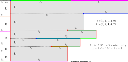
Figure 1: A rectangular decomposition of an Abelian differential with two zeros of angle $4\pi$ each on a Riemann surface of genus 2. Each $R_{i+1}$ contains a singularity on its top edge, at a distance $x_{i}$ from $J$, $1\leq i\leq n-1.$ The $x_{i}$ specify the gluing entirely.

Number the rectangles $R_{1},\dots,R_{n}$. We can define an $n\times n$ matrix $A$ of non-negative integers whose $(i,j)$th entry $a_{i,j}$ is the number of times $f(R_{i})$ crosses $R_{j}$. This matrix $A$ will be our main focus. The thinner rectangles are nicely stacked within the $R_{i}$ as each component of $f(R_{i})$ crosses $R_{j}$ from one end to the other, since it does not contain a singularity in its interior.

Proposition 1.1.

The leading eigenvalue of $A$ is the dilatation $\lambda$ of $f$. The vectors

$$\text{of lengths }\quad{\bf l}=\begin{pmatrix}l_{1}\\ \vdots\\ l_{n}\end{pmatrix}\quad\text{and of heights\ \quad{\bf h}=}\begin{pmatrix}h_{1}\\ \vdots\\ h_{n}\end{pmatrix}$$

are eigenvectors of $A$ and $A^{\top}$ with eigenvalue $\lambda$ respectively:

$$A{\bf l}=\lambda{\bf l}\quad\text{and}\quad A^{\top}{\bf h}=\lambda{\bf h}.$$

Proof.

The sum $\sum_{j}a_{i,j}l_{j}$ is exactly the length of $f(R_{i})$, i.e., $\lambda l_{i}=\sum_{j}a_{i,j}l_{j}$. Thus $\lambda{\bf l}=A{\bf l}$.

Similarly, $\sum_{i}a_{i,j}h_{i}$ is the sum of the heights of the $f(R_{i})$ crossing $R_{j}$, each of height $h_{i}/\lambda$. This leads to $h_{j}=\sum_{i}a_{j,i}(h_{j}/\lambda)$. Thus $\lambda{\bf h}=A^{\top}{\bf h}$.

∎

2 Combinatorial: ordered block permutations

This paper addresses the following question: what combinatorial data is needed to specify a $q$-rectangular decomposition for some pseudo-Anosov homeomorphism? We will deal only with OF pseudo-Anosov homeomorphisms.

Definition 2.1.

A pseudo-Anosov homeomorphism $f$ for the quadratic differential $q$ is OF (oriented fixed) if $q=\omega^{2}$ is the square of an Abelian differential, so that the invariant foliations are orientable, and such that all the singularities and all the critical trajectories emanating from the singularities are fixed by $f$.

Assume $X$ is a Riemann surface of genus $g>0$ and $\omega$ is a holomorphic $1$-form on $X$ with $\nu$ zeros of multiplicities $p_{1},\dots,p_{\nu}$, carrying an OF pseudo-Anosov homeomorphism. In this case there is a natural way to order the rectangles.

Imagine we have drawn $J$ with $z_{0}$ at the top and $z_{1}$ at the bottom. Then each rectangle is glued along its vertical left edge on the right side of $J$. In a translated chart, each rectangle is also glued on the left of $J$, along the right vertical edge. We order them $R_{1},\dots,R_{n}$ from top to bottom as on the right of $J$, and define the permutation $\sigma$ by saying that $R_{i}$ is in position $\sigma(i)$ on the left. Thus, if seen to the left of $J$, the top-most rectangle is $R_{\sigma^{-1}(1)}$.

The union of the rectangles $R_{1},\dots,R_{n}$ drawn on the right of $J$ is a chart covering the whole surface. By construction, $\forall i=1,\dots,(n-1)$, the intersection $R_{i}\cap R_{i+1}$ corresponds to an incoming critical horizontal trajectory drawn from a point of $J$ to a singularity $X_{i}$, after which it continues as two different outgoing horizontal trajectories, one as the bottom-right of $R_{i}$ and one as the top-right of $R_{i+1}$. Thus we have drawn $n-1$ incoming horizontal trajectories in the surface. If there is a singularity on the bottom horizontal edge of $R_{n}$, covering a sector of angle $0$ to $\pi$ around it, there is another place (the top of some other rectangle) where the rest of the angle is covered (as all identifications are done by translations). Thus this incoming horizontal trajectory from $J$ to the critical set has already been accounted for in the $n-1$.

On the other hand, at a zero of multiplicity $p_{i}$, there are $p_{i}+1$ incoming horizontal trajectories. Thus, since $p_{1}+\cdots+p_{\nu}=-\chi(X)=2g-2$, we see that

$$n-1=\sum_{i=1}^{\nu}(p_{i}+1)=2g+\nu-2.$$

$$\text{Thus,}\quad n=2g+\nu-1.$$

.

In fact, since $1\leq\nu\leq 2g-2$, we see that

$$2g\leq n\leq 4g-3\quad\quad\&\quad\quad\frac{n+3}{4}\leq g\leq n/2.$$

For instance, a genus $2$ surface may only appear in such a description with $n=4$ or $5$ rectangles. And a rectangular decomposition with $n=7$ rectangles, can only be a surface of genus $2.5\leq g\leq 3.5$, so only $g=3$.

Under the pseudo Anosov $f$, the image of $J$ is the smaller sub-segment $f(J)$, containing the fixed $z_{0}$. Each rectangle $R_{i}$ gets stretched by $\lambda$ horizontally and shrunk by $\lambda$ vertically. Then starting from its left edge on $f(J)$, $f(R_{i})$ starts as the $i^{\text{th}}$ thinner rectangle and continues following the gluings along $J$, passes $J\setminus f(J)$ many times (without containing a drawn critical horizontal trajectory in its interior) but stops eventually on a right edge glued to $f(J)$. We think of these thinner rectangles as strands - components of $X\setminus(J\cup f(\Gamma))$. No strand intersects more than one $R_{i}$, as otherwise $R_{i}$ would contain a critical point in its interior.

Say the number of strands that pass through $R_{i}$ is $k_{i}$. Then ${\bf k}\in\mathbb{N}^{n}$, together with $\sigma$ specify $(X,\omega)$ upto (independent) horizontal and vertical scaling and also specify the OF homeo $f$, as we shall see below (see Thm. 3.1). We study the bigger permutation on the strands defined by the vertical gluings given by $\sigma$. Here $\mathbb{N}=\{1,2,...\}$, and $\mathbb{N}_{n}=\{1,2,...,n\}$.

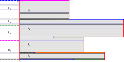
Figure 2: A rectangular decomposition of an Abelian differential with one zero of angle $6\pi$ on a Riemann surface of genus 2. The 4 rectangles are glued on the left of $J$ in a different order. $f$ takes rectangle $R_{i}$ to a collection of thinner sub-rectangles; the image of $R_{4}$ is shaded darker. Here $\sigma=(4,1,3,2),\,{\bf k}=(6,5,4,3)$.

We shall give a purely combinatorial way of describing the data of these rectangles. Let $\sigma\in\operatorname{Perm}(n)$ be a permutation of $\mathbb{N}_{n}$. Let ${\bf k}=k_{1},\dots,k_{n}$ be positive integers, and set $K=k_{1}+\cdots+k_{n}$.

Partition the ordered set $(1,\dots,K)$ into blocks $B_{1},\dots,B_{n}$, where $B_{1}$ consists of the ordered set of the first $k_{1}$ integers $(1,\dots,k_{1})$, $B_{2}$ contains the next $k_{2}$ elements $(k_{1}+1,\dots,k_{1}+k_{2})$, and in general for $1\leq i\leq n$ we have $B_{i}=(1+\sum_{j<i}k_{j},\dots,\sum_{j\leq i}k_{j})$. We will call the elements of $(1,\dots,K)$ strands (they correspond to the intersections $f(R_{j})\cap R_{i}$, ordered as they appear on the right side of $J$). If the strand $j\in(1,\dots,K)$ belongs to block $B_{i}$, we define $\beta(j)=i$, $\beta:(1,\dots,K)\to(1,\dots,n)$.

To the left of $J$, the rectangle $R_{i}$ appears in position $\sigma(i)$. The strands in block $B_{i}$, thus appear on the left in the $\sigma(i)^{\text{th}}$-block. This defines a permutation $\tau_{\sigma,\mathbf{k}}=\tau:(1,\dots,K)\rcirclearrowleft$, which we call an ordered block permutation (OBP). If we think of the ordered set $\{1,...,K\}$ as the set of sets $\{B_{1},...,B_{n}\}$, then the OBP $\tau$ simply reorders the subsets $B_{i}$ according to $\sigma$. I.e. $\tau$ reorders it as $\{B_{\sigma^{-1}(1)},...,B_{\sigma^{-1}(n)}\}$, while leaving the ordering within the $B_{i}$ untouched.

Definition 2.2.

The ordered block permutation (OBP) $\tau=\tau_{\sigma,{\bf k}}$ is a permutation of the set $(1,\dots,K=\sum_{i=1}^{n}k_{i})$ defined by

$$\tau_{\sigma,{\bf k}}(j):=j+\sum_{1\leq i<\sigma(\beta(j))}k_{\sigma^{-1}(i)}-\sum_{1\leq i<\beta(j)}k_{i}$$

Thus an OBP is a combinatorial way to describe an Interval Exchange Transformation (IET) in the sense of [V82] for instance. In fact, flowing $J$ at constant speed along $\partial_{x}$ until each piece hits $J$ again is the IET, and the OBP $\tau$ encodes this combinatorially.

Just as $\sigma$ tell us where the right side of $R_{i}$ is to be glued on the left of $J$, $\tau$ can be thought of as encoding where to glue the right side of the $i^{th}$ strand when we glue it to a strand on the left of $J$. Note that if $1\leq j\leq K$ is in block $i=\beta(j)$, then strand $j$ is the $(j-\sum_{1\leq i<\beta(j)}k_{i})^{th}$ strand of the block $B_{i}$. Also on the left side of $J$, the number of strands are in the order $(k_{\sigma^{-1}(1)},\cdots,k_{\sigma^{-1}(n)})$. Thus $\tau_{\sigma,{\bf k}}$ sends the $j$th strand of the $i$th block to the $j$th strand of the block on the left in position $\sigma(i)$.

When this data comes from an OF pA map, a strand $i$ among the first $n$, $1\leq i\leq n$, has its vertical right side glued to the left side of strand $\tau(i)$. Continuing this way, the right side of strand $\tau(i)$ is glued to the left side of strand $\tau(\tau(i))$. This continues until some $m_{i}>1$ such that $1\leq\tau^{\circ m_{i}}(i)\leq n$. Then the right vertical boundary of strand $\tau^{\circ(m_{i}-1)}(i)$ is not entirely glued to the left side of strand $\tau^{\circ m_{i}}(i)$, but the gluing is given by a copy of the bigger picture, $R_{i}$ on the right and $R_{\sigma(i)}$ on the left of $J$, scaled down vertically by $\lambda$.

Thus for each $1\leq i\leq n$, the collection of the $m_{i}$ strands, $\{i,...,\tau^{\circ(m_{i}-1)}(i)\}$ of the $\tau$ orbit of $i$ correspond precisely to the image of rectangle $R_{i}$ under the pA $f$. We call this ordered set of numbers $O_{i}:=(i,...,\tau^{\circ(m_{i}-1)}(i))$ the orbit of $i=1,...,n$. Clearly the orbits $O_{i}$ are disjoint.

Remark 2.1.

Note that as a permutation, an admissible OBP $\tau$ has as many cycles as $\sigma$, hence less than $n$. A cycle of $\tau$ containing $i$ consists of the ordered union of the orbits $O_{i}\cup O_{\sigma(i)}\cup...\cup O_{\sigma^{-1}(i)}$. In fact $\tau$ can be thought of as an enlargement of the permutation $\sigma$, where each arrow $i\to\sigma(i)$ is replaced by the orbit $O_{i}$.

Remark 2.2.

If we instead look to the left of $J$ and flip the horizontal foliation, obtaining the conjugate surface $\bar{X}$, the permutation $\sigma$ and the vector $\mathbf{k}=(k_{i})_{i=1}^{n}$ of positive integers, change to $\sigma^{-1}$ and $(k_{\sigma^{-1}(i)})_{i=1}^{n}$. The corresponding OBP $\tau_{\sigma^{-1},k_{\sigma^{-1}(*)}}$ is just the inverse $(\tau_{\sigma,\mathbf{k}})^{-1}$. The orbit of $\sigma^{-1}(i)$ continues as the orbit of $i$ backwards, without the $i$, $i$ being it’s first return under $\tau^{-1}$. The corresponding matrix is $(A_{\sigma^{-1}(i),\sigma^{-1}(j)})_{i,j=1}^{n}$, it is also a non-negative symplectic matrix, in fact $A_{\tau^{-1}}=P_{\sigma}AP_{\sigma}^{-1}$ where $P_{\sigma}$ is the permutation matrix $(\mathbf{e}_{\sigma(1)},\cdots,\mathbf{e}_{\sigma(n)})$, with $P_{\sigma^{-1}}=P_{\sigma}^{-1}=P_{\sigma}^{\top}$.

Figure 3: This figure represents the two possibilities for the NS edge of $\Gamma$ (purple): it might be the bottom edge of $R_{n}$ (left) or the bottom edge of $R_{\sigma^{-1}}(n)$ (right). The green rectangle is the one which contains $z_{1}$ in its top. In the left figure, on the left of $J$ it is the rectangle immediately beneath $R_{n}$, which appears in position $\sigma(n)+1$, so it is $R_{\sigma^{-1}(\sigma(n)+1)}$. On the right, it appears immediately beneath $R_{\sigma^{-1}(n)}$ so it is rectangle $R_{\sigma^{-1}(n)+1}$.

3 Admissible OBPs

The definition of admissible is purely combinatorial. Set $\tau^{\prime}=\tau^{\prime}_{\sigma,{\bf k}}:(1,...,n)\rcirclearrowleft$ to be the first return map under iteration of $\tau$ to the subset $(1,...,n)\subset(1,...,K)$. I.e. $\tau^{\prime}(i)=\tau^{\circ m_{i}}(i)$, where $m_{i}>1$ is the smallest index such that $1\leq\tau^{\circ m_{i}}(i)\leq n$.

The entry $a_{ij}$ in the $i^{th}$ row and the $j^{th}$ column of $A$ counts how many strands in the $j^{th}$ block $B_{j}$ are in the $i^{th}$ orbit $O_{i}$. That is, $a_{ij}$ is the number of elements in the intersection:

$$a_{ij}\quad=\quad|O_{i}\cap B_{j}|$$

Entries in the $i^{\text{th}}$-row of $A$ add up to $m_{i}$, i.e. the length of the orbit $O_{i}$, i.e. the number of strands in the image of $R_{i}$; the $j^{\text{th}}$-column of $A$ adds up to $k_{j}$, the number of strands that pass $R_{j}$.

Note that when the OBP $\tau$ is obtained from an OF pA map, the first return map $\tau^{\prime}$ equals the permutation $\sigma$. Since each critical vertical trajectory is fixed too, the image $f(R_{i})$ (or $O_{i}$) passes at least once as the top and once as the bottom strand of $R_{i}$ itself. The only exception to this is that one bottom edge of either $R_{n}$ or $R_{\sigma^{-1}(n)}$, the NS edge, doesn’t contain a singularity. The strand above the NS edge in fact belongs to the image of the other of the two ($R_{n}$ or $R_{\sigma^{-1}(n)}$), which isn’t NS. This is since $z_{1}$ is not a singular point and $\lambda>1$.

The top and bottom strands of each block $B_{i}$ are the least and biggest elements of the block, namely strands number $\sum_{j<i}k_{j}+1$ and $\sum_{j\leq i}k_{j}$.

Definition 3.1.

An ordered block permuation $\tau=\tau_{\sigma,\mathbf{k}}$ is admissible if

1. $\cup_{i=1}^{n}O_{i}=\{1,\dots,K\}$;

2. $\tau^{\prime}_{\sigma,{\bf k}}(i)=\sigma(i),\quad\forall 1\leq i\leq n$;

3. The matrix $A$ defined by $a_{ij}=|O_{i}\cap B_{j}|$ is irreducible;

4. Each orbit $O_{i}$ includes the top and bottom strand of $B_{i}$, except that the bottom strands of both $B_{\sigma^{-1}(n)}$ and $B_{n}$, namely strands $\{\tau^{-1}(K),K\}$, belong to just one of the two orbits: to $O_{\sigma^{-1}(n)}$, when the singularity is to the left of $z_{1}$; or to $O_{n}$, singularity to the right of $z_{1}$;

5. OBP $\tau$ is right-admissible if the NS edge is to the right of $z_{1}$, left-admissible if to the left. When right-admissible, for each $i=1,...,n-1$ except $i=\sigma^{-1}(1)-1$ the following holds: If $\sigma(i+1)=\sigma(n)+1$ then $\sigma(i)\neq n$ and otherwise $\sigma(i+1)\neq\sigma(i)+1$. For $z_{0}$: if $\sigma(1)=\sigma(n)+1$ then $\sigma^{-1}(1)\neq\sigma^{-1}(n)+1$ and otherwise $\sigma^{-1}(\sigma(1)-1)\neq\sigma^{-1}(1)-1$. In the (left-admissible) case, the same conditions above are satisfied by $\sigma^{-1}$.

Condition (v) rules out regular fixed points appearing as conical singularities $X_{i}$ (see proof of Thm.) Though in all the examples we’ve computed, condition (iii) is automatically satisfied, we cannot yet prove that it follows.

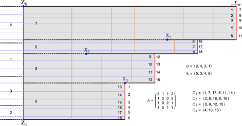
Figure 4: The red $J$ extended along the orange vertical line forms the full preimage of $J$. Call the components of any $R_{i}\setminus f^{-1}(J)$ tiles. Each tile maps to a strand by a linear homeomorphism. On the (solid) slits to the right of the $X_{i}$, the gluing is determined by how the rectangles arrive to the left of $J$. This figure is the right-admissible conjugate of fig. 2.

Lemma 3.1.

Some properties of an admissible OBP $\tau=\tau_{\sigma,\mathbf{k}}$.

1. $k_{1}\geq n$ and $k_{\sigma^{-1}(1)}\geq n$.

2. $\sigma(1)>1$ and $\sigma(n)<n$.

3. Denote by $\mathbf{k}_{\sigma^{-1}}$ the vector $\{k_{\sigma^{-1}(1)},...,k_{\sigma^{-1}(n)}\}$. Then $\sigma^{-1},\mathbf{k}_{\sigma^{-1}}$ define the OBP $\tau^{-1}$ which is also admissible. One of the two OBPs, $\tau$ or $\tau^{-1}$, is left-admissible and one is right-admissible. $\tau$ corresponds to an OF pA map on $(X,\omega)$ iff $\tau^{-1}$ does on $(\bar{X},\bar{\omega})$.

4. When right-admissible: $\forall i\in\mathbb{N}_{n}\setminus\{\sigma^{-1}(n)\}$, the orbit $O_{i}$ does not contain the top or bottom strand of a block $B_{j},\,\,\forall j\in\mathbb{N}_{n}\setminus\{i\}$. The orbit $O_{\sigma^{-1}(n)}$ contains the bottom strand of $B_{n}$ - strand $K$ - in addition to the top and bottom of $B_{\sigma^{-1}(n)}$.

Proof.

.

3. The OBP corresponding to $\sigma^{-1},\mathbf{k}_{\sigma^{-1}}$ reorders the blocks $B_{\sigma^{-1}(1)},...,B_{\sigma^{-1}(n)}$ to $B_{1},...,B_{n}$, without changing the order within the blocks. If $\tau$ is admissible, the $\tau^{-1}$ orbit of one of its first $n$ strands consists of the orbit of $i$ backwards and without $i$. The orbits of the two being the same, the $n$ orbits of $\tau^{-1}$ cover all strands. The first return $(\tau^{-1})^{\prime}$ is equal to $\sigma^{-1}$. Orbit of $i$ contains the first and last elements of the block $B_{\sigma^{-1}(i)}$ with the exception that only one of the two, $O_{n}$ or $O_{\sigma^{-1}(n)}$, contain both the bottom strands, $\tau^{-1}(K)$ and $K$. Thus $\tau^{-1}$ is admissible and of the other type (left or right) as $\tau$.

Considering $\sigma^{-1}$ and $(k_{\sigma^{-1}(i)})_{i=1}^{n}$ simply corresponds to looking at $f$ on the same surface from the other of its two possible orientations. If one of $\tau,\tau^{-1}$ provides rectangles that glue to form a surface or provide an OF pA map of it, so does the other, by taking the conjugate rectangles and the same map.

For part 1, if $n>k_{1}$ then the $k_{1}+1$-strand is in orbit $O_{2}$ and also $O_{k_{1}+1}$ since it is one of the first $n$ strands. So $k_{1}=1$, but if only one strand passes through $R_{1}$ then $\lambda=1$. Considering $\tau^{-1}$ gives $n\leq k_{\sigma^{-1}(1)}$. For 2, note that $\sigma(1)=1$ or $\sigma(n)=n$ would imply the $\tau$ orbits of $1,...,n$ do not include all the strands, contradicting part (i) of admissible.

Part 4 follows from the fact that each orbit $O_{i}$ contains the top and bottom strands of $B_{i}$, except that $O_{n}$ doesn’t contain the bottom strand of $B_{n}$, strand $K$, which belongs to $O_{\sigma^{-1}(n)}$. ∎

Example 3.1.

Let $n=4$ and $\sigma=\begin{pmatrix}1&2&3&4\\ 4&2&1&3\end{pmatrix}$. Set $k_{1}=4,k_{2}=3,k_{3}=6,k_{4}=9$, so that $K=22$. The permutation $\tau_{\sigma,{\bf k}}$ is

$$\ \ 1\ \ 2\ \ \ 3\ \ \ 4\ \ \ 5\ \ 6\ \ 7\ \ 8\ \ 9\ 10\ 11\ 12\ 13\ 14\ 15\ 16\ 17\ 18\ 19\ 20\ 21\ 22$$

$$\ 19\ 20\ 21\ 22\ \ \ 7\ \ 8\ \ 9\ \ 1\ \ 2\ \ 3\ \ \ 4\ \ \,5\ \ 6\ \,10\ 11\ 12\ 13\ 14\ 15\ 16\ 17\ 18$$

Why are $\tau_{\sigma,{\bf k}}(1,2,3,4)=(19,\ 20,\ 21,\ 22)$? The block $\sigma(1)$ is the fourth block, so strand j of the first block maps to the strand $j$ of the fourth block, which is strand $18+j$.

The orbits are

$$O_{1} ={\color[rgb]{0,1,0}1},19,15,11,[{\color[rgb]{1,0,0}4}]$$

$$O_{2} =2,20,16,12,{\color[rgb]{0,1,0}5},{\color[rgb]{1,0,0}7},9,[2]$$

$$O_{3} =3,21,17,{\color[rgb]{1,0,0}13},6,{\color[rgb]{0,1,0}8},[1]$$

$$O_{4} =4,{\color[rgb]{1,0,0}22},18,{\color[rgb]{0,1,0}14},10,[3],$$

where we have colored in red in each $O_{i}$ the bottom strand of $B_{i}$ and in green the top strand.

The union of the orbits is indeed all $22$ strands, and the permutation $\tau^{\prime}_{\sigma,{\bf k}}$ is $\begin{pmatrix}1&2&3&4\\ 4&2&1&3\end{pmatrix}$ which is indeed $\sigma$. So combinatorially, $(\sigma,{\bf k})$ is indeed an admissible block permutation. Note that indeed $4$ is not in orbit $O_{1}$, and $4$ is the bottom strand of $B_{1}$. We are in the case where $1=\sigma^{-1}(4)=\sigma^{-1}(n)$, case left-admissible.

We can now state our main result.

Theorem 3.1.

Let $\sigma$ be a permutation on $n$ letters, and $\mathbf{k}$ a vector of $n$ positive integers such that $\tau_{\sigma,{\bf k}}$ is an admissible OBP. Let $A$ be the corresponding $n\times n$ matrix, with leading eigenvalue $\lambda$. Choose positive eigenvectors ${\bf l}$ for $A$ and ${\bf h}$ for $A^{\top}$, and let $R_{1},\dots,R_{n}$ be rectangles with $R_{i}$ of size $l_{i}\times h_{i}$, in fact identified with $[0,l_{i}]\times[0,h_{i}]\subset{\mathbb{R}}^{2}$. The rectangles fit together to give a genus $g$ Riemann surface $X$ with a holomorphic $1$-form $\omega$, and the maps

$$x+iy\mapsto\lambda x+i\frac{y}{\lambda}$$

in each rectangle fit together to give an OF pseudo-Anosov homeomorphism $f_{\sigma,{\bf k}}:X\to X$. The genus is bounded $\frac{1}{4}(n+3)\leq g\leq\frac{1}{2}n$, and equals $(n+1-\nu)/2$, where $\nu$ is the number of distinct singularities.

Conversely, if $f:X\to X$ is an OF pA homeomorphism of a R.S. of genus $g$, the choice of a singularity $z_{0}$ and of a vertical segment $\tilde{J}$ of any length, emanating from $z_{0}$, defines an admissible OBP of size $n$, bounded $2g\leq n\leq 4g-3$, and equal to $2g+\nu-1$.

Proof.

Let us first see the converse, i.e., that the admissibility conditions are met if we construct an $\omega^{2}$-rectangular decomposition for an OF pseudo-Anosov homeomorphism as above.

The first condition is satisfied since the union $\bigcup R_{i}$ is the whole surface, so is the union $\bigcup_{i}f(R_{i})$. The second condition expresses that $f(J)=J^{\prime}$, so everything you see for blocks along $J$ has to be true of strands along $J^{\prime}$. Condition (iii) is more than satisfied, the matrix $A$ is aperiodic or mixing ($A^{n}$ has strictly positive entries).

Condition (iv) expresses that all the singularities, and all the leaves emanating from singularities, are fixed by $f$. Thus the singularity on the bottom of $R_{i}$ must also be on the bottom of $f(R_{i})$, so $f(R_{i})$ must contain that point as the bottom of some strand, and similarly for the top.

This argument doesn’t hold for the NS edge, which is the bottom edge of either $R_{n}$ or $R_{\sigma^{-1}(n)}$ since the NS edge emanates from $z_{1}$. Whether the singularity is to the left or right of $z_{1}$, both final strands to the left and right of $J$, strands number $\tau^{-1}(K)$ and $K$ belong to the orbit of the rectangle containing the singularity, since $\lambda>1$. Thus one of $O_{n}$ or $O_{\sigma^{-1}(n)}$ contain both strands $\tau^{-1}(K),K$.

Part (v) is a consequence of our construction of the rectangular decomposition using singular points of angle $\geq 4\pi$. If one of the points were fake, i.e. of angle $2\pi$ and merely fixed, the condition would fail: first, the gluings on the vertical edges are clear, thus when we say top-right edge of a rectangle $R_{i}$, we mean the horizontal part of its top boundary, to the right of the singularity. Similarly define the top-left, bottom-right, bottom-left for each rectangle.

Consider the right-admissible case. Rectangles $R_{1},...,R_{n-1}$ have a singularity in the interior of their bottom edge, by construction of the rectangular decomposition. $R_{1}$ has a singularity at the top-left corner, and $R_{\sigma^{-1}(1)}$ has a singularity at the top-right corner, and the other rectangles have a singularity in the interior of their top edge. $R_{n}$ has no singularity on its bottom edge.

As for the identifications, looking to the right of $J$, $R_{i}$ and $R_{i+1}$ are identified along $x_{i}$, the bottom-left of $R_{i}$ and the top-left of $R_{i+1}$, for $i=1,\dots,n-1$. To the left of $J$, define edges $y_{1},\dots,y_{n-1}$ as the top-right edge of $R_{\sigma^{-1}(2)},\dots,R_{\sigma^{-1}(n)}$ respectively, (since each rectangle except $R_{\sigma^{-1}(1)}$ has a top-right). The top = top-left of $R_{\sigma^{-1}(1)}$ is $x_{\sigma^{-1}(1)-1}\in\{x_{1},\dots,x_{n-1}\}$ and $y_{0}:=0$ as the empty ‘top-right’ of the first rectangle on the left. Finally label the bottom-right of $R_{\sigma^{-1}(n)}$ as $y_{n}$.

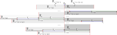
Figure 5: Right-admissible OBPs: The top-right edge of $R_{\sigma^{-1}(1+\sigma(n))}$ is glued first to the bottom-right of $R_{\sigma^{-1}(n)}$ and the rest past $z_{1}$ to the bottom of $R_{n}$. This figure corresponds to case $\sigma(1)\neq\sigma(n)+1$, so $R_{n}$ isn’t directly above $R_{1}$.

For $i=1,\dots,n-1$, the top-right of the $(i+1)^{st}$ rectangle on the left of $J$, i.e. $y_{i}$, is identified to the bottom-right of the $i^{th}$ rectangle to the left of $J$, (of $R_{\sigma^{-1}(i)}$). The only exception to this is $y_{\sigma(n)}$. As can be seen to the left of $J$ on $y_{\sigma(n)}$ (or below $z_{1}$, see Fig. 5 below), $y_{\sigma(n)}=$ the top-right of $R_{\sigma^{-1}(1+\sigma(n))}$ is identified to the union of $y_{n}$ and the NS edge, which is the bottom of $R_{n}$, of length $l_{n}$. These are all the identifications. Let $X_{0}:=z_{0}$, then the singularity $X_{\sigma^{-1}(1+\sigma(n))-1}$ is identified to $X_{\sigma^{-1}(n)}$.

First consider $z_{0}$ to be fake. The top of $R_{1}$ is glued to the bottom-right of $R_{\sigma^{-1}(\sigma(1)-1)}$, unless that happens to be $R_{n}$ (which happens iff $\sigma(1)=\sigma(n)+1$), in which case it is glued first to the bottom right $R_{\sigma^{-1}(n)}$, and the rest of it to the bottom of $R_{n}$ past $z_{1}$. Meanwhile the top of $R_{\sigma^{-1}(1)}$ is always glued to the bottom left of $R_{\sigma^{-1}(1)-1}$. Thus if $\sigma(1)=\sigma(n)+1$, we get $R_{\sigma^{-1}(n)}$ is glued to the top of $R_{1}$, so $z_{0}$ is fake iff $\sigma^{-1}(1)=\sigma^{-1}(n)+1$. If $\sigma(1)\neq\sigma(n)+1$, $z_{0}$ is fake iff $\sigma(\sigma^{-1}(1)-1)=\sigma(1)-1$. We remark here that in the last relation, if we switch every $\sigma$ with $\sigma^{-1}$ and vice versa, we obtain the same relation.

Now consider $X_{i}$ with $i=1,...,n-1$ but not $X_{\sigma^{-1}(1)-1}=z_{0}$. Then above the top-right of $R_{i+1}$ is the bottom-right of some rectangle. Again, either $\sigma(i+1)=\sigma(n)+1$ or not. If so, $X_{i}$ is fake iff $\sigma(i)=n$ and if not $X_{i}$ is fake iff $\sigma(i+1)=\sigma(i)+1$.

In the left-admissible case, we stipulate that $\sigma^{-1}$ satisfy the condition above. If the conjugate surface $\bar{X}$ has a fake point, so will $X$. This ends the proof of the converse.

Now we prove the direct statement: that if $\tau_{\sigma,{\bf k}}$ is an admissible OBP, then rectangles $R_{i}$ can be glued together to form a surface carrying a 1-form and an OF pseudo-Anosov homeomorphism. We will assume here that the OBP $\tau$ is right-admissible, which suffices by Lemma 3.1(3).

The first thing to specify is the size of the rectangles. From an admissible OBP we can build an $n\times n$ matrix of non-negative integers $A$: $a_{i,j}$ is the number of strands of orbit $O_{i}$ in the $j$th block $B_{j}$, or $|O_{i}\cap B_{j}|$.

Let $\lambda>1$ be the leading eigenvalue of $A$, let ${\bf l}$ be a positive $\lambda$-eigenvector, i.e., $A{\bf l}=\lambda{\bf l}$, and let ${\bf h}$ be a positive $\lambda$-eigenvector for $A^{\top}$, i.e., $A^{\top}{\bf h}=\lambda{\bf h}$. Both of these are guaranteed to exist by Perron-Frobenius, and defined up to independant scaling by a positive real.

We have now constructed the rectangles of lengths $l_{i}$ and heights $h_{i}$. The next task is to determine the identifications on their boundaries. The vertical identifications are determined by $\sigma$. As for the horizontal edges: $x_{i},1\leq i\leq n-1$, will denote the edge along which rectangles $R_{i}$ and $R_{i+1}$ are glued on the right of $J$, (and with slight abuse of notation $x_{i}$ will also denote the length of $x_{i}$). An admissible $\tau$ determines the image $f(R_{i})$ through the orbit $O_{i}$, and in particular tells us exactly when it crosses the top strand of $R_{i},\forall 2\leq i\leq n$. Denote by $O^{\prime}_{i}$ the part of the $i$th orbit $O_{i}$ before the top strand of $R_{i}$, $i=2,...,n$, after which the top strand (strand no. $\sum_{r=1}^{i-1}k_{r}+1$) is crossed, and the rest of the orbit as $O^{\prime\prime}_{i}$. Thus $O_{i}=O^{\prime}_{i}\sqcup\{\sum_{r=1}^{i-1}k_{r}+1\}\sqcup O^{\prime\prime}_{i}$.

Each $x_{i}$ is to be stretched by $\lambda$ under $f$ (encoded in $\tau$). The images of rectangles $R_{i}$ and $R_{i+1}$ start as strands $i$ and $i+1$ inside $R_{1}$ (as $k_{1}\geq n$), and then pass the same sequence of rectangles, $\{R_{\beta(j)}\}_{j\in O^{\prime}_{i+1}}$. [This follows since adjacent strands $i,i+1$ stay adjacent under $\tau$ exactly until the fixed $X_{i}$ passes between them, since otherwise orbit $O_{i+1}$ would contain the top strand of some other $B_{j},\,j\neq i+1$ which is impossible for a top strand by Lemma 3.1(4).] Thus we don’t have to worry about $x_{i}$ being defined as the bottom-left edge of $R_{i}$ or the top-left edge of $R_{i+1}$. After passing the fixed $X_{i}$, the images continue as the bottom strand of $R_{i}$ and the top strand of $R_{i+1}$, and the two strands diverge into different rectangles for the rest of their images. Looking at the orbit of $R_{i+1}$ until it crosses its top strand we want $\lambda x_{i}=\sum_{j\in O^{\prime}_{i+1}}l_{\beta(j)}+x_{i}$ and this determines $x_{i}$ as

$$x_{i}=\frac{1}{\lambda-1}\sum_{j\in O^{\prime}_{i+1}}l_{\beta(j)}\,,\quad\quad i=1,\dots,n-1.$$

Now, by choice of $\mathbf{l}$ as the $\lambda$-eigenvector, we know that $(A{\bf l})_{i+1}=\lambda l_{i+1}$, and the part on the left can be decomposed into the orbits before and after the top strand of $R_{i+1}$ is crossed, thus giving us:

$$\sum_{j\in O^{\prime}_{i+1}}l_{\beta(j)}+l_{i+1}+\sum_{j\in O^{\prime\prime}_{i+1}}l_{\beta(j)}=\lambda l_{i+1}$$

Which upon rearranging gives, for $i=1,...,n-1$:

$$\underbrace{\frac{1}{\lambda-1}\sum_{j\in O^{\prime}_{i+1}}l_{\beta(j)}}_{\text{$x_{i}$}}+\underbrace{\frac{1}{\lambda-1}\sum_{j\in O^{\prime\prime}_{i+1}}l_{\beta(j)}}_{\text{$y_{\sigma(i+1)-1}$}}=l_{i+1}$$

Where $y_{\sigma(i+1)-1}$, determined by the formula above, is the top-right edge of $R_{i+1}$. This list includes $y_{0}$ when $i=\sigma^{-1}(1)-1\in\{1,\dots,n-1\}$. i.e. when $R_{i+1}=R_{\sigma^{-1}(1)}$, and $O^{\prime\prime}_{i+1}$ is empty (since $\tau^{\prime}=\sigma$), and $y_{\sigma(i+1)-1}=y_{0}=0$ so $x_{\sigma^{-1}(1)-1}=l_{\sigma^{-1}(1)}$ and the cone point is at the top-right corner of $R_{i+1}=R_{\sigma^{-1}(1)}$. Otherwise, if $\sigma(i+1)>1$, then after crossing the top strand of $R_{i+1}\neq R_{\sigma^{-1}(1)}$, the orbit must continue to cross $R_{\sigma^{-1}(1)}$ so as to end to the left of $R_{1}$ (as $k_{\sigma^{-1}(1)}\geq n$ also). Therefore in this case $O^{\prime\prime}_{i+1}\neq\emptyset$ and thus $\forall i\in\mathbb{N}_{n-1}\setminus\{\sigma^{-1}(1)-1\}$ we have $0<\,x_{i}\,<l_{i+1}$ and $0<\,y_{\sigma(i+1)-1}\,<l_{i+1}$. This list of positive $y_{\sigma(i+1)-1}$ is the list $y_{1},...,\widehat{y_{\sigma(1)-1}},...,y_{n-1}$, where the skipped term $y_{\sigma(1)-1}$, is the entire top edge of $R_{1}$. But this has length $l_{1}$, also positive.

The only horizontal edge left to be determined is $y_{n}:=$ the bottom-right of the last rectangle on the left of $J$, but this requires decomposing the orbits of $R_{i}$ according to when the bottom strand is crossed, $i=1,\dots,n-1$. One obtains a different decomposition of the orbit $O_{i}$, (as some $O^{(3)}_{i}\sqcup\{\sum_{j=1}^{i}k_{j}\}\sqcup O^{(4)}_{i}$), but the part before the bottom strand, $O^{(3)}_{i}$, still goes through the rectangles $\{R_{\beta(j)}\}_{j\in O^{\prime}_{i+1}}$, by Lemma 3.1(4) as above. We obtain,

$$x_{i}+y_{\sigma(i)}=l_{i}\,,\quad i=1,...,n-1.$$

Where we decomposed the bottom edges of $R_{1},\dots,R_{n-1}$. The list of $y$’s here is the list $y_{1},\dots,\widehat{y_{\sigma(n)}},\dots,y_{n}$, which definitely includes $y_{n}$ since $\sigma(n)<n$. We have $y_{n}>0$ since if the part of the orbit defining it was empty, then this orbit would end in $R_{\sigma^{-1}(n)}$, but orbits only end in $R_{\sigma^{-1}(1)}\neq R_{\sigma^{-1}(n)}$. Now except for $y_{n}$ and $y_{\sigma(n)}$, the other $y$’s have been defined twice. For each $j=1,\dots,\widehat{\sigma(n)},\dots,n-1,\quad y_{j}$ has been defined once according to the orbit of $R_{\sigma^{-1}(j+1)}$ after it’s top strand and once according to the orbit of $R_{\sigma^{-1}(j)}$ after it’s bottom strand. These two sets of strands can be run backwards starting as the $j^{th}$ and $j+1^{st}$ strands of $R_{\sigma^{-1}(1)}$ and follow the same sequence of rectangles again by Lemma 3.1(4), showing that the new definition for these $y$’s coincides with the previous definition.

As for the case of $y_{n}$ and $y_{\sigma(n)}$ containing the NS edge, we subtract the two previous equations and get

$$y_{\sigma(i+1)-1}-y_{\sigma(i)}=l_{i+1}-l_{i}\,,\quad\quad i=1,\dots,n-1.$$

Adding over $i$ yields,

$$\left(\sum_{i=1}^{n-1}y_{i}-y_{\sigma(1)-1}\right)-\left(\sum_{i=1}^{n-1}y_{i}+y_{n}-y_{\sigma(n)}\right)=\sum_{i=1}^{n-1}(l_{i+1}-l_{i})=l_{n}-l_{1}.$$

And since $y_{\sigma(1)-1}=l_{1}$, we get: $\framebox{$\displaystyle y_{\sigma(n)}=y_{n}+l_{n}$}$, which shows that $y_{\sigma(n)}>l_{n}$, so $R_{n}$ falls short of $y_{\sigma(n)}$ as it lies above $y_{\sigma(n)}$ to the left of $J$.

To sum up, so far, after a choice of ${\bf l}$ and ${\bf h}$, as above for an admissible OBP $\tau$, all the $x_{i}$ are determined, and satisfy $0<x_{i}<l_{i}$ and $x_{i}<l_{i+1}$ except $x_{\sigma^{-1}(1)-1}$ which equals $l_{\sigma^{-1}(1)}$. The rest of the horizontal edges, $y_{1},\dots,y_{n}$ are also uniquely determined and positive, smaller in length than the two rectangles that contain them.

Since $y_{\sigma(n)}=y_{n}+l_{n}$, the bottom edge of $R_{n}$ can be glued to the top edge of $R_{\sigma^{-1}(1+\sigma(n))}$, starting from the right and the rest of the top edge of $R_{\sigma^{-1}(1+\sigma(n))}$ can be glued to the bottom of $R_{\sigma^{-1}(n)}$ starting from the right, and they fit. This takes care of all the gluings, and all points have topological disks as neighborhoods. $z_{0}$ and the $X_{i}$ are singular points of angle $2\pi q,\,q\geq 2$ so we obtain a Riemann surface with an Abelian differential.

The map $f$ defined by the orbits of the strands is a homeomorphism: the collection of strands in $O_{i}$ form a connected long and thin rectangle in the surface, of size $\lambda l_{i}\times\frac{h_{i}}{\lambda}$. The interior of $R_{i}$ can be sent homeomorphically to this long and thin rectangle. A small neighborhood of a point on the edge $x_{i}$ is homeomorphically sent to a small neighborhood of its image as strands $i,i+1$ travel together until $X_{i}$ is fixed. Similarly for the $y_{i}$ looking to the left of $J$. Finally, one can check around the fixed singularities, that $f$ is indeed a homeomorphism.
∎

The matrices $A$ of size $2g+\nu-1$ one obtains in the construction above are “symplectic”: Define $\gamma_{i}$ to be the closed curve in the surface running down the middle of $R_{i}$ with its right end-point connected to its initial point along $J$. Then $\gamma_{1},...,\gamma_{n}$ form a spanning set for the homology group $H_{1}(X,\mathbb{Z})$ of size $2g$. Let $S$ be the intersection matrix of the $\gamma_{i}$. Then $S_{ii}=0$ and if $\sigma$ preserves the relative order of $i$ and $j$, then $S_{ij}=S_{ji}=0$. If $\sigma$ reverses their relative order, $S_{ij}$ is $+1$ above the diagonal and $-1$ below. $S$ is the intersection form, expressed in terms of a spanning set rather than a basis (unless $\nu=1$) of the homology. Moreover, we see that $(ASA^{\top})_{i\,j}$ equals the number of points in $f(\gamma_{i})\cap f(\gamma_{j})$ and therefore equals $S_{i\,j}$. So

$$ASA^{\top}=S$$

and the dilatation $\lambda$ is the eigenvalue of a non-negative irreducible integer matrix $A$, which isn’t of size $2g$ necessarily, but of size $n=2g+\nu-1$.

We remark also that the Perron root $\lambda$ associated to an OBP $\tau$ satisfies both

$$\min_{1\leq i\leq n}\{k_{i}\}<\lambda<\max_{1\leq i\leq n}\{k_{i}\},$$

$$\min_{1\leq i\leq n}\{m_{i}\}<\lambda<\max_{1\leq i\leq n}\{m_{i}\}.$$

Acknowledgements: We would like to thank Sylvain Bonnot and Arcelino do Nascimento for helpful discussions.

References:

• ] Hubbard, John and Howard Masur. “Quadratic differentials and foliations.” Acta Mathematica 142.1 (1979): 221-274.

• ] Rafiqi, Ahmad. “On dilatations of surface automorphisms.” Cornell University PhD Thesis (2018).

• ] Veech, William A. “Gauss Measures for Transformations on the Space of Interval Exchange Maps.” Annals of Mathematics Vol. 115, no. 2, (1982), pp. 201–242.