Power spectrum modelling of galaxy and radio intensity maps including observational effects

Abstract

Fluctuations in the large-scale structure of the Universe contain significant information about cosmological physics, but are modulated in survey datasets by various observational effects. Building on existing literature, we provide a general treatment of how fluctuation power spectra are modified by a position-dependent selection function, noise, weighting, smoothing, pixelization and discretization. Our work has relevance for the spatial power spectrum analysis of galaxy surveys with spectroscopic or accurate photometric redshifts, and radio intensity-mapping surveys of the sky brightness temperature including generic noise, telescope beams and pixelization. We consider the auto-power spectrum of a field, the cross-power spectrum between two fields and the multipoles of these power spectra with respect to a curved sky, deriving the corresponding power spectrum models, estimators, errors and optimal weights. We note that “FKP weights” for individual tracers do not in general provide the optimal weights when measuring the cross-power spectrum. We validate our models using mock datasets drawn from N-body simulations. Our treatment should be useful for modelling and studying cosmological fluctuation fields in observed and simulated datasets.

1 Introduction

The power spectrum of the large-scale structure of the Universe – and its dependence on scale, redshift and direction – contains significant information about the composition of the Universe and the cosmological physics governing the growth of structure with time. Modern cosmological surveys can trace this large-scale structure over large volumes, by mapping the individual redshift-space positions of galaxies or quasars, the cumulative brightness temperature of spectral emission in a region of sky using intensity mapping in radio wavebands, or the spectral absorption of background light by intervening matter.

One of the central problems in cosmological analysis is to relate these measured fluctuations in probes of large-scale structure, which are modulated by various observational effects and analysis approximations, to the underlying matter power spectrum which encodes the important cosmological information. Relevant observational effects may include a variation in the mean background level of the fields as a function of position (the survey selection function or mask), noise due to the sampling of discrete objects or in the measured brightness temperature, or smoothing of the fields in the mapping process due to the telescope resolution. Analysis approximations may involve the pixelization or gridding technique employed, and wide-angle corrections to the local plane-parallel approximation.

Moreover, we may also utilize the cross-correlation between two different observed fields which trace the same underlying matter fluctuations. Such a multi-tracer analysis offers several benefits: (1) uncorrelated noise components in the two fields will bias the amplitude of their auto-power spectra, but not their cross-power spectrum; (2) an additive systematic component afflicting one of the fields will appear in its auto-correlation but not the cross-correlation; (3) if the fields trace a common sample variance of matter fluctuations, such that their measurement errors are correlated, then the noise in some joint derived parameters will be reduced (Seljak, 2009).

A valuable example of the ability of cross-correlation to mitigate systematic errors arises in the joint analysis of 21-cm intensity mapping performed by radio telescopes and galaxy redshift surveys. Even if intensity-mapping surveys are afflicted by significant residual components of foreground emission, cross-correlation will allow the neutral hydrogen content of galaxies to be studied (Wolz et al., 2016). Auto- and cross-correlation studies of current intensity-mapping datasets, which are still limited by areal coverage, noise and foregrounds, are presented by Chang et al. (2010), Masui et al. (2013), Wolz et al. (2017) and Anderson et al. (2018). The scientific possibilities of radio intensity mapping will be greatly expanded by facilities such as the Canadian Hydrogen Intensity Mapping Experiment (CHIME, Bandura et al., 2014), the Hydrogen Intensity and Real-time Analysis eXperiment (HIRAX, Newburgh et al., 2016), the Tianlai Cylinder Array (Xu et al., 2015) and the BINGO telescope (Wuensche & the BINGO Collaboration, 2018), leading up to Phase 1 of the Square Kilometre Array (Square Kilometre Array Cosmology Science Working Group et al., 2018).

The imprint of observational effects in the galaxy power spectrum has been widely modelled in the literature. Peacock & Nicholson (1991) described the additive and multiplicative effects of a survey mask on the observed Fourier coefficients of the density field. These results were extended by Feldman et al. (1994) who, starting from a general model of the galaxy density field including clustering, Poisson noise and survey selection, derived power spectrum estimators, covariance and optimal weights. These weights were extended by Percival et al. (2004) to include the dependence of clustering on luminosity, and by Smith & Marian (2015) to encapsulate the population of halos by galaxies. Related treatments of the cross-power spectrum between two galaxy tracers were presented by Smith (2009) and Blake et al. (2013). Jing (2005) modelled the effect on the estimated power spectrum of how fields are assigned to a Fast Fourier Transform (FFT) grid (see also, Cui et al., 2008) and Sefusatti et al. (2016) demonstrated the technique of interlacing to compensate for aliasing. Much recent work has focussed on modelling the multipoles of the power spectrum with respect to a varying line-of-sight direction (Yamamoto et al., 2006; Beutler et al., 2014; Wilson et al., 2017; Beutler et al., 2017; Castorina & White, 2018; Blake et al., 2018).

Our work aims to review and extend these previous results by providing a general formalism relating the 2-point statistics of fluctuations in Fourier space to various observational effects. This framework may be applied to galaxy and intensity-mapping surveys, other 3D cosmological maps, and their cross-correlation. In particular, we extend the literature by deriving the imprint on the auto- and cross-power spectra of smoothing or pixelization schemes which depend on position. Such effects are particularly relevant for radio intensity maps, which may include a telescope beam, frequency channels and angular pixelization across a curved sky. We also extend the results of Feldman et al. (1994) to intensity mapping correlations and cross-correlations, by considering the general optimal weighting of fields in auto- and cross-power spectrum measurements.

Our paper is structured as follows. In Section 2 we present models for the imprint of observational effects on the fluctuation power spectra. After some introductory definitions (Sections 2.1, 2.2), we start by reviewing the relations between the Fourier transform of the fluctuation fields and their underlying power spectra, including the effects of a position-dependent selection function, noise and weights, and considering both auto- and cross-power spectra (Section 2.3). We then derive the impact on the fluctuation power spectra if the fields are smoothed or pixelized in a manner varying with position, for example by a telescope beam, redshift errors, a spherical pixelization scheme or nearest grid-point assignment (Section 2.4). We also review the effect of the discretization of the fields onto an FFT grid (Section 2.5). Finally, we summarize how the power spectra may be analysed in terms of their multipoles with respect to a varying line-of-sight (Section 2.6). In Section 3, we review the estimators for the auto- and cross-power spectra and their multipoles (Section 3.1) and the variance in these estimators under certain approximations, and we derive the general optimal weighting of the fluctuation fields for measurement of these different power spectra, providing examples for galaxy and intensity-mapping surveys and their cross-correlation (Section 3.2). In Section 4 we validate our models by computing the observed and predicted multipole power spectra of mock galaxy and intensity-mapping datasets drawn from an N-body simulation, including a variety of observational effects. We summarize our results in Section 5.

2 Power spectrum modelling

2.1 Fourier conventions

For clarity of the subsequent derivations, we start by noting the conventions we adopt for the Fourier transform of a function $f(\textbf{{x}})$:

$$\tilde{f}(\textbf{{k}})=\frac{1}{V}\int d^{3}\textbf{{x}}\,f(\textbf{{x}})\,e^{i\textbf{{k}}.\textbf{{x}}},\hskip 28.45274ptf(\textbf{{x}})=\frac{V}{(2\pi)^{3}}\int d^{3}\textbf{{k}}\,\tilde{f}(\textbf{{k}})\,e^{-i\textbf{{k}}.\textbf{{x}}},$$ (1)

such that $f(\textbf{{x}})$ and $\tilde{f}(\textbf{{k}})$ have the same units, and where $V$ is the volume of the enclosing Fourier cuboid. We define dimensionless Dirac delta functions $\delta_{D}$ in configuration and Fourier space such that,

$$\tilde{\delta}_{D}(\textbf{{k}})=\frac{1}{V}\int d^{3}\textbf{{x}}\,e^{i\textbf{{k}}.\textbf{{x}}},\hskip 28.45274pt\delta_{D}(\textbf{{x}})=\frac{V}{(2\pi)^{3}}\int d^{3}\textbf{{k}}\,e^{i\textbf{{k}}.\textbf{{x}}},$$ (2)

which are applied to functions such that,

$$\frac{1}{V}\int d^{3}\textbf{{x}}\,f(\textbf{{x}})\,\delta_{D}(\textbf{{x}}-\textbf{{x}}_{0})=f(\textbf{{x}}_{0}),\hskip 28.45274pt\frac{V}{(2\pi)^{3}}\int d^{3}\textbf{{k}}\,\tilde{f}(\textbf{{k}})\,\tilde{\delta}_{D}(\textbf{{k}}-\textbf{{k}}_{0})=\tilde{f}(\textbf{{k}}_{0}).$$ (3)

2.2 Fluctuation fields

We now provide some definitions related to fluctuation fields, their correlation functions and power spectra. Consider a function $\delta(\textbf{{x}})$ which represents the fluctuations of a field $f(\textbf{{x}})$ with position x, relative to its mean “background” value across many realizations of an ensemble (indicated by angled brackets) such that,

$$\delta(\textbf{{x}})=f(\textbf{{x}})-\langle f(\textbf{{x}})\rangle,$$ (4)

and $\langle\delta(\textbf{{x}})\rangle=0$. The field could represent the galaxy number density distribution $f(\textbf{{x}})=V\,n_{g}(\textbf{{x}})$ (which is dimensionless) or HI brightness temperature $f(\textbf{{x}})=T_{b}(\textbf{{x}})$ (with dimensions of temperature). In a simple linear bias model neglecting redshift-space distortions, the fluctuations in galaxy number density and temperature may be described by,

$$n_{g}(\textbf{{x}})=\langle n_{g}(\textbf{{x}})\rangle\,\left[1+b_{g}\,\delta_{m}(\textbf{{x}})\right],\hskip 28.45274ptT_{b}(\textbf{{x}})=\langle T_{b}(\textbf{{x}})\rangle\,\left[1+b_{HI}\,\delta_{m}(\textbf{{x}})\right],$$ (5)

where $b_{g}$ and $b_{HI}$ are the linear bias of the galaxies and HI-emitting objects, respectively, and $\delta_{m}$ is the underlying matter overdensity. Hence the corresponding fluctuations are:

$$\delta_{g}(\textbf{{x}})=\langle n_{g}(\textbf{{x}})\rangle\,b_{g}\,\delta_{m}(\textbf{{x}}),\hskip 28.45274pt\delta_{T}(\textbf{{x}})=\langle T_{b}(\textbf{{x}})\rangle\,b_{HI}\,\delta_{m}(\textbf{{x}}).$$ (6)

The dimensionless auto-correlation function of the field between two positions x and $\textbf{{x}}^{\prime}$ with separation $\textbf{{s}}=\textbf{{x}}-\textbf{{x}}^{\prime}$, assuming statistical homogeneity, is defined by,

$$\xi(\textbf{{s}})=\frac{\langle f(\textbf{{x}})\,f(\textbf{{x}}^{\prime})\rangle-\langle f(\textbf{{x}})\rangle\,\langle f(\textbf{{x}}^{\prime})\rangle}{\langle f(\textbf{{x}})\rangle\,\langle f(\textbf{{x}}^{\prime})\rangle}=\frac{\langle\delta(\textbf{{x}})\,\delta(\textbf{{x}}^{\prime})\rangle}{\langle f(\textbf{{x}})\rangle\,\langle f(\textbf{{x}}^{\prime})\rangle}.$$ (7)

Re-arranging Equation 7 and adding uncorrelated noise to the field with variance $\sigma^{2}(\textbf{{x}})$ as a function of position, the 2-point statistics of the fluctuations can be written in the form,

$$\langle\delta(\textbf{{x}})\,\delta(\textbf{{x}}^{\prime})\rangle=\langle f(\textbf{{x}})\rangle\,\langle f(\textbf{{x}}^{\prime})\rangle\,\xi(\textbf{{x}}-\textbf{{x}}^{\prime})+\sigma^{2}(\textbf{{x}})\,\delta_{D}(\textbf{{x}}-\textbf{{x}}^{\prime}).$$ (8)

Similarly, the cross-correlation of two fluctuation fields $\delta_{1}(\textbf{{x}})=f_{1}(\textbf{{x}})-\langle f_{1}(\textbf{{x}})\rangle$ and $\delta_{2}(\textbf{{x}})=f_{2}(\textbf{{x}})-\langle f_{2}(\textbf{{x}})\rangle$, assuming that the noise in the fields is uncorrelated, is given by,

$$\langle\delta_{1}(\textbf{{x}})\,\delta_{2}(\textbf{{x}}^{\prime})\rangle=\langle f_{1}(\textbf{{x}})\rangle\,\langle f_{2}(\textbf{{x}}^{\prime})\rangle\,\xi_{c}(\textbf{{x}}-\textbf{{x}}^{\prime}),$$ (9)

in terms of the cross-correlation function $\xi_{c}(\textbf{{s}})$.

The correlation functions of the fields may be related to their auto-power spectra $P(\textbf{{k}})$ and cross-power spectra $P_{c}(\textbf{{k}})$ by,

$$P(\textbf{{k}})=\int d^{3}\textbf{{s}}\,\xi(\textbf{{s}})\,e^{i\textbf{{k}}.\textbf{{s}}},\hskip 28.45274ptP_{c}(\textbf{{k}})=\int d^{3}\textbf{{s}}\,\xi_{c}(\textbf{{s}})\,e^{i\textbf{{k}}.\textbf{{s}}},$$ (10)

defined here in volume units ($h^{-3}$ Mpc³), including the appropriate temperature unit for the intensity map. As exemplified by Equation 6, our measured fields trace fluctuations in the matter overdensity $\delta_{m}(\textbf{{x}})$, which we model in terms of the matter power spectrum $P_{m}(\textbf{{k}})$. For the purposes of this study we assume that the redshift-space power spectra of the fields, in the absence of any observational effects, may be described by a simple 3-parameter redshift-space distortion model (Hatton & Cole, 1998) combining the large-scale Kaiser effect (Kaiser, 1987) imprinted by the growth rate $f$, exponential damping from random pairwise velocities with dispersion $\sigma_{v}$, and a linear bias $b$:

$$P(\textbf{{k}})=P(k,\mu)=\frac{(b+f\mu^{2})^{2}\,P_{m}(k)}{1+\left(k\mu\sigma_{v}/H_{0}\right)^{2}},\hskip 28.45274ptP_{c}(\textbf{{k}})=P_{c}(k,\mu)=\frac{(b_{1}+f\mu^{2})\,(b_{2}+f\mu^{2})\,P_{m}(k)}{1+\left(k\mu\sigma_{v}/H_{0}\right)^{2}},$$ (11)

where $\mu$ is the cosine of the angle between k and the line-of-sight.

In the following subsections we build a model connecting the Fourier transform of the observed fluctuation fields to their underlying auto-power spectra $P(\textbf{{k}})$ and cross-power spectra $P_{c}(\textbf{{k}})$, which contains cosmological information as described by Equation 11. We include a number of practical observational and measurement effects:

• A selection function which varies with position, $\langle f(\textbf{{x}})\rangle=\langle n_{g}(\textbf{{x}})\rangle V$ or $\langle f(\textbf{{x}})\rangle=\langle T_{b}(\textbf{{x}})\rangle$,

• Uncorrelated noise in the field as a function of position, described by $\sigma^{2}(\textbf{{x}})$ in Equation 8, including the specific example of Poisson noise,

• A weight $w(\textbf{{x}})$ applied to the field to optimize the signal-to-noise ratio of the measurement,

• A smoothing function which can vary with position, with specific examples provided for a Gaussian telescope beam, frequency channels in radio observations, redshift errors, HEALPix pixelization (Górski et al., 2005) and nearest grid point assignment,

• Discretization of the field onto an FFT grid.

2.3 Relating the fluctuation fields to the power spectra

We now develop the relationship between the observed fluctuations and their underlying power spectra, building on existing literature. We can relate the observed fluctuation fields to their power spectra by considering the Fourier transform of the weighted fields,

$$\tilde{\delta}(\textbf{{k}})=\frac{1}{V}\int d^{3}\textbf{{x}}\,w(\textbf{{x}})\,\delta(\textbf{{x}})\,e^{i\textbf{{k}}.\textbf{{x}}},$$ (12)

where $w(\textbf{{x}})$ is a general position-dependent weight which may be applied to optimize the signal-to-noise ratio of the measurement. The average of $|\tilde{\delta}(\textbf{{k}})|^{2}$ across realizations is,

$$\langle|\tilde{\delta}(\textbf{{k}})|^{2}\rangle=\frac{1}{V^{2}}\int d^{3}\textbf{{x}}\int d^{3}\textbf{{x}}^{\prime}\,w(\textbf{{x}})\,w(\textbf{{x}}^{\prime})\,\langle\delta(\textbf{{x}})\,\delta(\textbf{{x}}^{\prime})\rangle\,e^{i\textbf{{k}}.(\textbf{{x}}-\textbf{{x}}^{\prime})}.$$ (13)

Substituting in Equations 8 and 10 to Equation 13 we find, in a slight generalization of the results of Feldman et al. (1994) to include a general noise term,

$$\langle|\tilde{\delta}(\textbf{{k}})|^{2}\rangle=\int\frac{d^{3}\textbf{{k}}^{\prime}}{(2\pi)^{3}}\,P(\textbf{{k}}^{\prime})\,|\tilde{W}(\textbf{{k}}-\textbf{{k}}^{\prime})|^{2}+\frac{1}{V}\int d^{3}\textbf{{x}}\,w^{2}(\textbf{{x}})\,\sigma^{2}(\textbf{{x}})=P\star|\tilde{W}|^{2}+\overline{S},$$ (14)

where we have defined a window function $W(\textbf{{x}})=w(\textbf{{x}})\,\langle f(\textbf{{x}})\rangle$. Hence, $\langle|\tilde{\delta}(\textbf{{k}})|^{2}\rangle$ is the sum of the convolution (which we denote by $\star$) of the underlying power spectrum $P(\textbf{{k}})$ and $|\tilde{W}(\textbf{{k}})|^{2}$, and a noise term,

$$\overline{S}=\frac{1}{V}\int d^{3}\textbf{{x}}\,w^{2}(\textbf{{x}})\,\sigma^{2}(\textbf{{x}}).$$ (15)

Repeating this process for the Fourier transform of two different fluctuation fields (see also Smith, 2009; Blake et al., 2013), weighted by functions $w_{1}(\textbf{{x}})$ and $w_{2}(\textbf{{x}})$, we find that,

$$\langle\tilde{\delta}_{1}(\textbf{{k}})\,\tilde{\delta}_{2}^{*}(\textbf{{k}})\rangle=\int\frac{d^{3}\textbf{{k}}^{\prime}}{(2\pi)^{3}}\,P_{c}(\textbf{{k}}^{\prime})\,\tilde{W}_{1}(\textbf{{k}}-\textbf{{k}}^{\prime})\,\tilde{W}_{2}^{*}(\textbf{{k}}-\textbf{{k}}^{\prime})=P_{c}\star\tilde{W}_{1}\,\tilde{W}_{2}^{*},$$ (16)

where $W_{i}(\textbf{{x}})=w_{i}(\textbf{{x}})\,\langle f_{i}(\textbf{{x}})\rangle$. In an approximation where the power spectrum does not vary significantly over the width of $|\tilde{W}(\textbf{{k}})|^{2}$, such that we can take it outside the integral over $\textbf{{k}}^{\prime}$ in Equations 14 and 16, and using Parseval’s theorem $\frac{V}{(2\pi)^{3}}\int d^{3}\textbf{{k}}\,|\tilde{W}(\textbf{{k}})|^{2}=\frac{1}{V}\int d^{3}\textbf{{x}}\,W^{2}(\textbf{{x}})$, we find,

$$\langle|\tilde{\delta}(\textbf{{k}})|^{2}\rangle\approx\overline{Q}\,\frac{P(\textbf{{k}})}{V}+\overline{S},\hskip 28.45274pt\langle\tilde{\delta}_{1}(\textbf{{k}})\,\tilde{\delta}_{2}^{*}(\textbf{{k}})\rangle\approx\overline{Q}_{c}\,\frac{P_{c}(\textbf{{k}})}{V},$$ (17)

where we have defined dimensionless quantities,

$$\overline{Q}=\frac{1}{V}\int d^{3}\textbf{{x}}\,W^{2}(\textbf{{x}}),\hskip 28.45274pt\overline{Q}_{c}=\frac{1}{V}\int d^{3}\textbf{{x}}\,W_{1}(\textbf{{x}})\,W_{2}(\textbf{{x}}).$$ (18)

In the following subsections we consider two important special cases of fluctuation fields, which will be relevant in the subsequent analysis.

2.3.1 Poisson point process

If $f(\textbf{{x}})$ is generated by a Poisson point process from a galaxy number density distribution $n_{g}(\textbf{{x}})$, then $\xi(\textbf{{s}})=0$ and

$$\langle\delta(\textbf{{x}})\,\delta(\textbf{{x}}^{\prime})\rangle=V\,\langle n_{g}(\textbf{{x}})\rangle\,\delta_{D}(\textbf{{x}}-\textbf{{x}}^{\prime}),$$ (19)

and from the definition $\delta(\textbf{{x}})=V\left[n_{g}(\textbf{{x}})-\langle n_{g}(\textbf{{x}})\rangle\right]$,

$$\langle\delta(\textbf{{x}})\,\delta(\textbf{{x}}^{\prime})\rangle=V^{2}\left[\langle n_{g}(\textbf{{x}})\,n_{g}(\textbf{{x}}^{\prime})\rangle-\langle n_{g}(\textbf{{x}})\rangle\,\langle n_{g}(\textbf{{x}}^{\prime})\rangle\right].$$ (20)

To justify Equation 19, we can use $N=\int d^{3}\textbf{{x}}\,n_{g}(\textbf{{x}})$ and consider

$$\langle N^{2}\rangle=\int d^{3}\textbf{{x}}\int d^{3}\textbf{{x}}^{\prime}\langle n_{g}(\textbf{{x}})n_{g}(\textbf{{x}}^{\prime})\rangle=\int d^{3}\textbf{{x}}\int d^{3}\textbf{{x}}^{\prime}\left[\langle n_{g}(\textbf{{x}})\rangle\langle n_{g}(\textbf{{x}}^{\prime})\rangle+\frac{\langle n_{g}(\textbf{{x}})\rangle}{V}\delta_{D}(\textbf{{x}}-\textbf{{x}}^{\prime})\right]=\langle N\rangle^{2}+\int d^{3}\textbf{{x}}\langle n_{g}(\textbf{{x}})\rangle=\langle N\rangle^{2}+\langle N\rangle,$$ (21)

as expected from Poisson statistics. Comparing Equations 8 and 19, we identify $\sigma^{2}(\textbf{{x}})=V\,\langle n_{g}(\textbf{{x}})\rangle$ and hence assuming weight $w=1$,

$$\langle|\tilde{\delta}(\textbf{{k}})|^{2}\rangle=\overline{S}=\int d^{3}\textbf{{x}}\,\langle n_{g}(\textbf{{x}})\rangle=N.$$ (22)

2.3.2 Uniform window and noise

Suppose that a field is sampled from a constant mean $\langle f(\textbf{{x}})\rangle=f_{0}$ with a constant noise $\sigma^{2}(\textbf{{x}})=\sigma_{0}^{2}$, where the weight function $w(\textbf{{x}})$ takes the value $0$ (outside the footprint) or 1 (inside the footprint), such that $w^{2}(\textbf{{x}})=w(\textbf{{x}})$ and the observed volume is $V_{w}=\int d^{3}\textbf{{x}}\,w(\textbf{{x}})$. In this case, we find from Equations 15 and 18 that $\overline{S}=\sigma_{0}^{2}V_{w}/V$ and $\overline{Q}=f_{0}^{2}V_{w}/V$ such that Equation 17 takes the form,

$$\langle|\tilde{\delta}(\textbf{{k}})|^{2}\rangle=\frac{f_{0}^{2}V_{w}}{V^{2}}\left[P(\textbf{{k}})+\frac{V\sigma_{0}^{2}}{f_{0}^{2}}\right].$$ (23)

In this scenario, the equivalent power spectrum due to noise is hence the second term in the bracket,

$$P_{\rm noise}(\textbf{{k}})=\frac{V\sigma_{0}^{2}}{f_{0}^{2}}.$$ (24)

We note that for Poisson statistics, $f_{0}=Vn_{0}$ in terms of the number density $n_{0}$, and $\sigma_{0}^{2}=Vn_{0}$, such that $P_{\rm noise}=1/n_{0}$, as expected.

2.4 Smoothing

We now extend the power spectrum model to describe the effect of a general smoothing of the fields, such as might result from a telescope beam in radio observations, redshift errors in optical observations, or a general pixelization. We suppose that the smoothed fluctuation field $\delta^{sm}(\textbf{{x}})$ may be written in the form,

$$\delta^{sm}(\textbf{{x}})=\frac{1}{V}\int d^{3}\textbf{{x}}^{\prime}\,\delta(\textbf{{x}}^{\prime})\,B(\textbf{{x}}-\textbf{{x}}^{\prime},\textbf{{x}}),$$ (25)

where the dimensionless smoothing function $B$ is a compact function of the separation $\textbf{{x}}-\textbf{{x}}^{\prime}$, which may also vary with position x. The smoothing function is normalized such that $\frac{1}{V}\int d^{3}\textbf{{s}}\,B(\textbf{{s}},\textbf{{x}})=1$ for all x, and we define the Fourier transform of the smoothing function at each location as $\tilde{B}(\textbf{{k}},\textbf{{x}})=\frac{1}{V}\int d^{3}\textbf{{s}}\,B(\textbf{{s}},\textbf{{x}})\,e^{i\textbf{{k}}.\textbf{{s}}}$, where $\tilde{B}(\textbf{{k}}=0,\textbf{{x}})=1$. Substituting in these expressions we find that the Fourier transform of Equation 25 is,

$$\tilde{\delta}^{sm}(\textbf{{k}})=\int\frac{d^{3}\textbf{{k}}^{\prime}}{(2\pi)^{3}}\,\tilde{\delta}(\textbf{{k}}^{\prime})\int d^{3}\textbf{{x}}\,\tilde{B}(\textbf{{k}}^{\prime},\textbf{{x}})\,e^{i(\textbf{{k}}-\textbf{{k}}^{\prime}).\textbf{{x}}},$$ (26)

which reproduces the standard result of the convolution theorem, that $\tilde{\delta}^{sm}(\textbf{{k}})=\tilde{B}(\textbf{{k}})\,\tilde{\delta}(\textbf{{k}})$ if $B(\textbf{{s}},\textbf{{x}})$ is independent of position x. The power spectrum of the smoothed field is then,

$$\langle|\tilde{\delta}^{sm}(\textbf{{k}})|^{2}\rangle=\int\frac{d^{3}\textbf{{k}}^{\prime}}{(2\pi)^{3}}\langle|\tilde{\delta}(\textbf{{k}}^{\prime})|^{2}\rangle\int d^{3}\textbf{{s}}\,e^{i(\textbf{{k}}-\textbf{{k}}^{\prime}).\textbf{{s}}}\,\frac{1}{V}\int d^{3}\textbf{{x}}\,\tilde{B}(\textbf{{k}}^{\prime},\textbf{{x}})\,\tilde{B}^{*}(\textbf{{k}}^{\prime},\textbf{{x}}+\textbf{{s}}).$$ (27)

Assuming that the smoothing function varies more slowly than the clustering scale, we may utilize the approximation $\int d^{3}\textbf{{x}}\,\tilde{B}(\textbf{{k}},\textbf{{x}})\,\tilde{B}^{*}(\textbf{{k}},\textbf{{x}}+\textbf{{s}})\approx\int d^{3}\textbf{{x}}\,|\tilde{B}(\textbf{{k}},\textbf{{x}})|^{2}$. Following this approximation the integral over s produces a delta function in $\textbf{{k}}-\textbf{{k}}^{\prime}$, which leads to the result that,

$$\langle|\tilde{\delta}^{sm}(\textbf{{k}})|^{2}\rangle\approx\langle|\tilde{\delta}(\textbf{{k}})|^{2}\rangle\,\frac{1}{V}\int d^{3}\textbf{{x}}\,|\tilde{B}(\textbf{{k}},\textbf{{x}})|^{2}=\langle|\tilde{\delta}(\textbf{{k}})|^{2}\rangle\,D^{2}(\textbf{{k}}),$$ (28)

such that the power spectra (including both the signal and noise) are modulated by a damping function $D^{2}(\textbf{{k}})=\frac{1}{V}\int d^{3}\textbf{{x}}\,|\tilde{B}(\textbf{{k}},\textbf{{x}})|^{2}$, which is the volume average of $|\tilde{B}(\textbf{{k}},\textbf{{x}})|^{2}$. If a smoothed field $\delta_{1}^{sm}(\textbf{{x}})$ is correlated with an unsmoothed field $\delta_{2}(\textbf{{x}})$, the modulation of the resulting cross-power spectrum is,

$$\langle\tilde{\delta}_{1}^{sm}(\textbf{{k}})\,\tilde{\delta}_{2}^{*}(\textbf{{k}})\rangle\approx\langle\tilde{\delta}_{1}(\textbf{{k}})\,\tilde{\delta}_{2}^{*}(\textbf{{k}})\rangle\,\frac{1}{V}\int d^{3}\textbf{{x}}\,\tilde{B}(\textbf{{k}},\textbf{{x}}),$$ (29)

or for the cross-correlation of two fields smoothed with different functions $B_{1}(\textbf{{s}},\textbf{{x}})$ and $B_{2}(\textbf{{s}},\textbf{{x}})$,

$$\langle\tilde{\delta}_{1}^{sm}(\textbf{{k}})\,\tilde{\delta}_{2}^{sm\,*}(\textbf{{k}})\rangle\approx\langle\tilde{\delta}_{1}(\textbf{{k}})\,\tilde{\delta}_{2}^{*}(\textbf{{k}})\rangle\,\frac{1}{V}\int d^{3}\textbf{{x}}\,\tilde{B}_{1}(\textbf{{k}},\textbf{{x}})\,\tilde{B}_{2}^{*}(\textbf{{k}},\textbf{{x}}).$$ (30)

In the following subsections we consider some special cases of these results, which will be utilized in the subsequent N-body simulation tests.

2.4.1 Pixelization

A special case of the smoothing operation described by Equation 25 occurs when a field is pixelized into distinct “cells”, such that the average value of the field within each cell $i$ is assigned to all positions within the cell. This behaviour can be modelled if the field is averaged by a top-hat function centred on each pixel position $\textbf{{x}}_{i}$ such that,

$$\delta^{sm}(\textbf{{x}})=\sum_{i}\frac{1}{\Delta V_{i}}\,P_{i}(\textbf{{x}})\int_{{\rm cell}\,i}d^{3}\textbf{{x}}^{\prime}\,\delta(\textbf{{x}}^{\prime})=\frac{1}{V}\int_{\rm all}d^{3}\textbf{{x}}^{\prime}\delta(\textbf{{x}}^{\prime})\sum_{i}\frac{V}{\Delta V_{i}}\,P_{i}(\textbf{{x}})\,P_{i}(\textbf{{x}}^{\prime}),$$ (31)

where $\Delta V_{i}$ is the volume of the cell and $P_{i}(\textbf{{x}})=1$ if x is in cell $i$, and zero otherwise. We now define the cell window function $T_{i}(\textbf{{x}}-\textbf{{x}}_{i})=1$ if x is in cell $i$, and zero otherwise, and an offset function with respect to the pixel position, $\textbf{{e}}_{i}(\textbf{{x}})=\textbf{{x}}-\textbf{{x}}_{i}$. Hence we can identify by comparison with Equation 25,

$$B(\textbf{{x}}-\textbf{{x}}^{\prime},\textbf{{x}})=\sum_{i}\frac{V}{\Delta V_{i}}\,P_{i}(\textbf{{x}})\,T_{i}(\textbf{{x}}^{\prime}-\textbf{{x}}+\textbf{{e}}_{i}(\textbf{{x}})).$$ (32)

Taking the Fourier transform of this equation,

$$\tilde{B}(\textbf{{k}},\textbf{{x}})=\sum_{i}\frac{1}{\Delta V_{i}}\,P_{i}(\textbf{{x}})\int d^{3}\textbf{{s}}\,T_{i}(\textbf{{s}}+\textbf{{e}}_{i}(\textbf{{x}}))\,e^{i\textbf{{k}}.\textbf{{s}}}=\sum_{i}\frac{V}{\Delta V_{i}}\,P_{i}(\textbf{{x}})\,\tilde{T}_{i}(\textbf{{k}})\,e^{-i\textbf{{k}}.\textbf{{e}}_{i}(\textbf{{x}})}.$$ (33)

In order to interpret this equation, we note that $\tilde{T}_{i}(0)=\Delta V_{i}/V$ and $\tilde{T}_{i}(\textbf{{k}})$ is proportional to $\tilde{B}(\textbf{{k}},\textbf{{x}})$ at the position of cell $i$. Hence, pixelization results in a phase change in the Fourier transform such that,

$$\tilde{B}(\textbf{{k}},\textbf{{x}})\rightarrow\tilde{B}(\textbf{{k}},\textbf{{x}})\,e^{-i\textbf{{k}}.\textbf{{e}}(\textbf{{x}})}.$$ (34)

This behaviour does not change the value of $|\tilde{B}(\textbf{{k}},\textbf{{x}})|^{2}$, hence the overall effect on the auto-power spectrum can still be evaluated using Equation 28. However, the damping of the cross-power spectrum as computed by Equation 29 is changed by this type of smoothing, by the volume average of $e^{-i\textbf{{k}}.\textbf{{e}}(\textbf{{x}})}$. Given that the offsets $\textbf{{e}}(\textbf{{x}})$ will be distributed across space with the same profile as the cells, this volume average is well-approximated by $\tilde{B}^{*}(\textbf{{k}},\textbf{{x}})$. Therefore, even though only one of the two fields is smoothed, the cross-power spectrum is damped due to pixelization by approximately the same factor $D^{2}(\textbf{{k}})$ as the auto-power spectrum.

2.4.2 Noise applied to cells

We now consider a scenario where the noise in the fluctuation field is generated by drawing a random variable in a series of cells $i$ of volume $\Delta V_{i}$, with zero mean and variance $\sigma^{2}_{i}$. In this case, the 2-point statistics of the noise in Equation 8 is modified from $\langle\delta(\textbf{{x}})\,\delta(\textbf{{x}}^{\prime})\rangle=\sigma^{2}(\textbf{{x}})\,\delta_{D}(\textbf{{x}}-\textbf{{x}}^{\prime})$ to,

$$\langle\delta(\textbf{{x}})\,\delta(\textbf{{x}}^{\prime})\rangle=\sum_{i}\sigma_{i}^{2}\,P_{i}(\textbf{{x}})\,P_{i}(\textbf{{x}}^{\prime}),$$ (35)

such that the noise is uncorrelated between different cells. Substituting this relation in Equation 13 we find,

$$\langle|\tilde{\delta}(\textbf{{k}})|^{2}\rangle=\frac{1}{V^{2}}\sum_{i}\sigma_{i}^{2}\int d^{3}\textbf{{x}}\int d^{3}\textbf{{x}}^{\prime}\,w(\textbf{{x}})\,w(\textbf{{x}}^{\prime})\,P_{i}(\textbf{{x}})\,P_{i}(\textbf{{x}}^{\prime})\,e^{i\textbf{{k}}.(\textbf{{x}}-\textbf{{x}}^{\prime})}=\frac{1}{V^{2}}\sum_{i}\sigma_{i}^{2}\,w_{i}^{2}\,|\tilde{B}(\textbf{{k}},\textbf{{x}}_{i})|^{2}\,(\Delta V_{i})^{2},$$ (36)

after applying the same arguments as in the previous subsection, where $w_{i}$ is the weight applied to cell $i$. The noise power spectrum (Equation 15) including pixelization,

$$\langle|\tilde{\delta}(\textbf{{k}})|^{2}\rangle=\frac{1}{V}\int d^{3}\textbf{{x}}\,w^{2}(\textbf{{x}})\,\sigma^{2}(\textbf{{x}})\,|\tilde{B}(\textbf{{k}},\textbf{{x}})|^{2},$$ (37)

can then be recovered by comparison with Equation 36 if we define the appropriate noise variance,

$$\sigma^{2}(\textbf{{x}})=\frac{1}{V}\sum_{i}\sigma_{i}^{2}\,\Delta V_{i}\,P_{i}(\textbf{{x}}).$$ (38)

Poisson noise, $\sigma^{2}(\textbf{{x}})=V\langle n_{g}(\textbf{{x}})\rangle$, is obtained if $\sigma_{i}^{2}=V^{2}\langle n_{g,i}\rangle/\Delta V_{i}$, where $\langle n_{g,i}\rangle$ is the galaxy number density in cell $i$. This result will be useful in Section 4, for adding a Poisson noise component to model an intensity map constructed by binning a simulation catalogue of discrete objects in cells.

2.4.3 Telescope beam

For Gaussian smoothing perpendicular to the line-of-sight, such as would result from a radio telescope beam, we have a smoothing kernel $B(s_{\perp})\propto e^{-s_{\perp}^{2}/2\sigma_{\perp}^{2}}$ as a function of perpendicular spatial separation $s_{\perp}$, where $\sigma_{\perp}$ is the spatial standard deviation of the beam. The Fourier transform of this function is,

$$\tilde{B}_{\rm beam}(\textbf{{k}})=e^{-k_{\perp}^{2}\sigma_{\perp}^{2}/2},$$ (39)

where $k_{\perp}=k\sqrt{1-\mu^{2}}$ and $\mu$ is the cosine of the angle between k and the line-of-sight. Hence, the beam damps power at small perpendicular separations. For a beam of constant angular standard deviation $\sigma_{\theta}$ on the sky in units of radians, the corresponding spatial smoothing scale will vary with position as $\sigma_{\perp}(\textbf{{x}})=|\textbf{{x}}|\,\sigma_{\theta}$. In this case we would derive the damping factor using Equation 28 as,

$$D^{2}(\textbf{{k}})=\frac{1}{V}\int d^{3}\textbf{{x}}\,e^{-k_{\perp}^{2}\,|\textbf{{x}}|^{2}\,\sigma_{\theta}^{2}}.$$ (40)

2.4.4 Frequency channels

Smoothing in the radial direction results from the width of the frequency channels in which radio intensity mapping data is collected. For a frequency channel of spatial width $s_{\parallel}$ the Fourier transform of the top-hat assignment function is,

$$\tilde{B}_{\rm chan}(\textbf{{k}})=\frac{\sin{(k_{\parallel}s_{\parallel}/2)}}{k_{\parallel}s_{\parallel}/2},$$ (41)

where $k_{\parallel}=k\mu$. If the frequency width of the channel is $\Delta\nu$ then, for line measurements with rest frequency $\nu_{0}$ such that $\nu=\nu_{0}/(1+z)$, $s_{\parallel}(\textbf{{x}})=[c/H(z)]\,(1+z)^{2}\,(\Delta\nu/\nu_{0})$ in terms of the speed of light $c$ and Hubble parameter $H(z)$. In this case we would derive the damping factor using Equation 28 as,

$$D^{2}(\textbf{{k}})=\frac{1}{V}\int d^{3}\textbf{{x}}\,\left[\frac{\sin{(k_{\parallel}s_{\parallel}(\textbf{{x}})/2)}}{k_{\parallel}s_{\parallel}(\textbf{{x}})/2}\right]^{2}.$$ (42)

2.4.5 Redshift errors

Damping of power in the radial direction can also result from errors in measured galaxy redshifts, for example due to photometric redshift estimates with error $\Delta z$ (which may vary with redshift). Assuming that these errors are Gaussian, the Fourier transform of the smoothing kernel follows Equation 39,

$$\tilde{B}_{\Delta z}(\textbf{{k}})=e^{-k_{\parallel}^{2}\sigma_{\parallel}^{2}/2},$$ (43)

where $\sigma_{\parallel}(\textbf{{x}})=[c/H(z)]\,\Delta z$ is the spatial radial error in each location. In this case the overall damping factor can be computed using,

$$D^{2}(\textbf{{k}})=\frac{1}{V}\int d^{3}\textbf{{x}}\,e^{-k_{\parallel}^{2}\,\sigma_{\parallel}^{2}(\textbf{{x}})}.$$ (44)

Chaves-Montero et al. (2018) present a related investigation of the effect of photo-$z$ errors on multipoles of the baryon acoustic oscillation power spectrum.

2.4.6 Angular pixelization

A process of angular pixelization, for example using a scheme such as HEALPix (Górski et al., 2005), results in a damping of power as a function of $k_{\perp}$. The associated damping of the angular power spectrum $C_{\ell}$ of the field as a function of multipole $\ell$ can be expressed in terms of the pixel window function $W_{\rm ang}(\ell)$, such that the damping is described by $C_{\ell}\rightarrow C_{\ell}\,W_{\rm ang}^{2}(\ell)$ and

$$W_{\rm ang}^{2}(\ell)=\frac{4\pi}{2\ell+1}\sum_{m=-\ell}^{\ell}|w_{\ell m}|^{2},$$ (45)

where $w_{\ell m}=\int_{\rm pixel}d\Omega\,Y_{\ell m}(\Omega)$ is the spherical harmonic transform of a pixel in terms of the spherical harmonic functions $Y_{\ell m}$. In the case of a 3D survey smoothed using angular pixelization, the contribution to the damping factor at position x relative to the observer is determined by identifying $\ell=k_{\perp}|\textbf{{x}}|$ such that $\tilde{B}_{\rm ang}(\textbf{{k}},\textbf{{x}})=W_{\rm ang}(k_{\perp}|\textbf{{x}}|)$. In this case we would derive the damping factor for the 3D power spectrum as,

$$D^{2}(\textbf{{k}})=\frac{1}{V}\int d^{3}\textbf{{x}}\,W_{\rm ang}^{2}(k_{\perp}|\textbf{{x}}|).$$ (46)

2.4.7 Nearest grid point assignment

For nearest grid point assignment, the Fourier transform of the assignment function is,

$$\tilde{B}_{\rm NGP}(\textbf{{k}})=\frac{\sin{(k_{x}H/2)}}{(k_{x}H/2)}\,\frac{\sin{(k_{y}H/2)}}{(k_{y}H/2)}\,\frac{\sin{(k_{z}H/2)}}{(k_{z}H/2)},$$ (47)

where $H$ is the grid spacing (e.g., Jing, 2005). This special case will be useful in the following section.

2.5 Discretization

We now consider the effect on the power spectrum if a continuous field $\delta(\textbf{{x}})$, possibly having been smoothed using one of the schemes described in the previous section, is sampled on a regular FFT grid at positions $\textbf{{x}}_{\textbf{{n}}}=H\textbf{{n}}$, where n is a vector of integers. This case is important for efficient power spectrum estimators. Following Jing (2005), we can conveniently describe this process using the sampling function $\Pi(\textbf{{x}})=\sum_{\textbf{{n}}}\delta_{D}(\textbf{{x}}-\textbf{{n}})$, an array of $\delta$-functions placed at integers n, such that the gridded field $\delta^{gr}(\textbf{{x}})$ can be written in the form,

$$\delta^{gr}(\textbf{{x}})=\Pi(\textbf{{x}}/H)\,\delta(\textbf{{x}}).$$ (48)

We can see that Equation 48 produces the correct result for the Fourier-transformed field by considering,

$$\tilde{\delta}^{gr}(\textbf{{k}})=\frac{1}{V}\int d^{3}\textbf{{x}}\,\delta^{gr}(\textbf{{x}})\,e^{i\textbf{{k}}.\textbf{{x}}}=\sum_{\textbf{{n}}}\frac{1}{V}\int d^{3}\textbf{{x}}\,\delta_{D}(\textbf{{x}}-\textbf{{n}}H)\,\delta(\textbf{{x}})\,e^{i\textbf{{k}}.\textbf{{x}}}=\sum_{\textbf{{n}}}\delta(\textbf{{x}}_{\textbf{{n}}})\,e^{i\textbf{{k}}.\textbf{{x}}_{\textbf{{n}}}},$$ (49)

as expected when evaluating an FFT. The Fourier transform of Equation 48 may also be obtained using the convolution theorem,

$$\tilde{\delta}^{gr}(\textbf{{k}})=\frac{V}{(2\pi)^{3}}\int d^{3}\textbf{{k}}^{\prime}\,\tilde{\delta}(\textbf{{k}}^{\prime})\,\tilde{\Pi}(\textbf{{k}}-\textbf{{k}}^{\prime}),$$ (50)

where the Fourier transform of the sampling function is given by,

$$\tilde{\Pi}(\textbf{{k}})=\frac{1}{V}\int d^{3}\textbf{{x}}\,\Pi(\textbf{{x}}/H)\,e^{i\textbf{{k}}.\textbf{{x}}}=\sum_{\textbf{{n}}}e^{i\textbf{{k}}.\textbf{{n}}H}=\sum_{\textbf{{n}}}e^{i2\pi\frac{\textbf{{k}}.\textbf{{n}}}{2k_{N}}}=\sum_{\textbf{{n}}}\tilde{\delta}_{D}(\textbf{{k}}-2k_{N}\textbf{{n}}),$$ (51)

where $k_{N}=\pi/H$ is the Nyquist frequency of the grid. Hence, Equation 50 may be simplified as,

$$\tilde{\delta}^{gr}(\textbf{{k}})=\sum_{\textbf{{k}}_{\textbf{{n}}}}\tilde{\delta}(\textbf{{k}}_{\textbf{{n}}}),$$ (52)

where $\textbf{{k}}_{\textbf{{n}}}=\textbf{{k}}+2k_{N}\textbf{{n}}$ such that,

$$\langle|\tilde{\delta}^{gr}(\textbf{{k}})|^{2}\rangle=\sum_{\textbf{{k}}_{\textbf{{n}}}}\langle|\tilde{\delta}(\textbf{{k}}_{\textbf{{n}}})|^{2}\rangle,$$ (53)

where cross-terms disappear because of homogeneity. Hence, discretization involves the aliasing of power to scale k from a series of scales $\textbf{{k}}_{\textbf{{n}}}$ spaced by $2k_{N}$ (Jing, 2005). Discretization is often combined with smoothing, in which case combining Equations 28 and 53 yields,

$$\langle|\tilde{\delta}^{gr}(\textbf{{k}})|^{2}\rangle=\sum_{\textbf{{k}}_{\textbf{{n}}}}\langle|\tilde{\delta}(\textbf{{k}}_{\textbf{{n}}})|^{2}\rangle\,D^{2}(\textbf{{k}}_{\textbf{{n}}}).$$ (54)

We note an interesting special case in which nearest grid point assignment is applied to a Poisson noise spectrum $\langle|\tilde{\delta}(\textbf{{k}})|^{2}\rangle=\overline{S}$, in which case the power spectrum is unchanged:

$$\langle|\tilde{\delta}^{gr}(\textbf{{k}})|^{2}\rangle=\overline{S}\,\sum_{\textbf{{k}}_{\textbf{{n}}}}D_{\rm NGP}^{2}(\textbf{{k}}_{\textbf{{n}}})=\overline{S},$$ (55)

where we have used the identity $\sum_{\textbf{{k}}_{\textbf{{n}}}}|\tilde{B}_{\rm NGP}(\textbf{{k}}_{\textbf{{n}}})|^{2}=1$, where $\tilde{B}_{\rm NGP}(\textbf{{k}})$ is defined by Equation 47.

Combining the results of the above sections, we can describe the joint effects of the window function, noise, smoothing and discretization on the auto-power spectrum of the fluctuation field by,

$$\langle|\tilde{\delta}(\textbf{{k}})|^{2}\rangle=\sum_{\textbf{{k}}_{\textbf{{n}}}}\left[(P\star|\tilde{W}|^{2})(\textbf{{k}}_{\textbf{{n}}})+\overline{S}\right]D^{2}(\textbf{{k}}_{\textbf{{n}}}),$$ (56)

and on the cross-power spectrum by,

$$\langle\tilde{\delta}_{1}(\textbf{{k}})\,\tilde{\delta}_{2}^{*}(\textbf{{k}})\rangle=\sum_{\textbf{{k}}_{\textbf{{n}}}}\left[(P_{c}\star\tilde{W}_{1}\tilde{W}_{2}^{*})(\textbf{{k}}_{\textbf{{n}}})\right]D^{2}(\textbf{{k}}_{\textbf{{n}}}).$$ (57)

2.6 Power spectrum multipoles

As the above sections demonstrate, the contribution of a fluctuation field to its power spectrum in a volume may vary as a function of x owing to variations in the statistical properties of the field such as its clustering, noise, smoothing or weighting. We can encapsulate these effects by writing the observed power spectrum as an integral over x,

$$P(\textbf{{k}})=\frac{1}{V}\int d^{3}\textbf{{x}}\,P(\textbf{{k}},\textbf{{x}}),$$ (58)

where $P(\textbf{{k}},\textbf{{x}})$ represents the contribution to the power spectrum originating from position x.

This concept is useful when considering a further cause of position-dependence: the changing line-of-sight direction across the volume. Effects such as redshift-space distortions, the telescope beam and angular/radial smoothing will cause the amplitude of the power spectrum $P(\textbf{{k}})$ to depend on the direction of k with respect to a global line-of-sight. Assuming azimuthal symmetry, the power spectrum will only depend on $\mu$, the cosine of the angle between k and the line-of-sight direction. In this case the 2D function $P(k,\mu)$ may be conveniently quantified by power spectrum multipoles, $P_{\ell}(k)$:

$$P(k,\mu)=\sum_{\ell}P_{\ell}(k)\,L_{\ell}(\mu)=\sum_{\ell}P_{\ell}(k)\,L_{\ell}(\hat{\textbf{{k}}}.\hat{\textbf{{x}}}),$$ (59)

where $L_{\ell}$ are the Legendre polynomials, and in the last expression we are describing the varying line-of-sight, given that in a region of space around position x from the observer we can write $\mu=\hat{\textbf{{k}}}.\hat{\textbf{{x}}}$. Inverting Equation 59 and averaging the statistic over all positions using Equation 58, we can model the power spectrum multipoles as,

$$\begin{split}P_{\ell}(k)&=\frac{2\ell+1}{V}\int d^{3}\textbf{{x}}\int\frac{d\Omega_{k}}{4\pi}\,P(\textbf{{k}},\textbf{{x}})\,L_{\ell}(\hat{\textbf{{k}}}.\hat{\textbf{{x}}})\\ &=(2\ell+1)\int\frac{d\Omega_{k}}{4\pi}\,\frac{1}{V}\int d^{3}\textbf{{x}}\int d^{3}\textbf{{x}}^{\prime}\,\xi(\textbf{{x}}-\textbf{{x}}^{\prime})\,e^{i\textbf{{k}}.(\textbf{{x}}-\textbf{{x}}^{\prime})}\,L_{\ell}(\hat{\textbf{{k}}}.\hat{\textbf{{x}}}^{\prime}),\end{split}$$ (60)

where $d\Omega_{k}$ integrates over all angles $\hat{\textbf{{k}}}$. The equivalent relation to Equation 13 for a power spectrum multipole $\ell$ can then be written as,

$$\langle|\tilde{\delta}(\textbf{{k}})|^{2}_{\ell}\rangle=\frac{1}{V^{2}}\int d^{3}\textbf{{x}}\int d^{3}\textbf{{x}}^{\prime}\,w(\textbf{{x}})\,w(\textbf{{x}}^{\prime})\,\langle\delta(\textbf{{x}})\,\delta(\textbf{{x}}^{\prime})\rangle\,e^{i\textbf{{k}}.(\textbf{{x}}-\textbf{{x}}^{\prime})}\,L_{\ell}(\hat{\textbf{{k}}}.\hat{\textbf{{x}}}^{\prime}),$$ (61)

where $\langle|\tilde{\delta}(\textbf{{k}})|^{2}_{\ell}\rangle$ describes the contribution of wavenumber k to the power spectrum multipole $P_{\ell}(k)$. Blake et al. (2018) develop the equivalent expressions to Equations 14 and 16 for modelling the auto- and cross-power spectrum multipoles. For the auto-power spectrum:

$$\langle|\tilde{\delta}(\textbf{{k}})|^{2}_{\ell}\rangle=\sum_{\ell^{\prime}}\int\frac{d^{3}\textbf{{k}}^{\prime}}{(2\pi)^{3}}\,P_{\ell^{\prime}}(k^{\prime})\,\tilde{W}(\textbf{{k}}-\textbf{{k}}^{\prime})\,W_{\ell\ell^{\prime}}^{*}(\textbf{{k}},\textbf{{k}}^{\prime})+\frac{1}{V}\int d^{3}\textbf{{x}}\,w^{2}(\textbf{{x}})\,\sigma^{2}(\textbf{{x}})\,L_{\ell}(\hat{\textbf{{k}}}.\hat{\textbf{{x}}}),$$ (62)

where

$$W_{\ell\ell^{\prime}}(\textbf{{k}},\textbf{{k}}^{\prime})=\frac{1}{V}\int d^{3}\textbf{{x}}\,W(\textbf{{x}})\,L_{\ell}(\hat{\textbf{{k}}}.\hat{\textbf{{x}}})\,L_{\ell^{\prime}}(\hat{\textbf{{k}}}^{\prime}.\hat{\textbf{{x}}})\,e^{i(\textbf{{k}}-\textbf{{k}}^{\prime}).\textbf{{x}}}.$$ (63)

The equivalent expression for the cross-power spectrum multipoles is,

$$\langle\tilde{\delta}_{1}(\textbf{{k}})\,\tilde{\delta}_{2}^{*}(\textbf{{k}})_{\ell}\rangle=\sum_{\ell^{\prime}}\int\frac{d^{3}\textbf{{k}}^{\prime}}{(2\pi)^{3}}\,P_{c,\ell^{\prime}}(k^{\prime})\,\tilde{W}_{1}(\textbf{{k}}-\textbf{{k}}^{\prime})\,W_{2,\ell\ell^{\prime}}^{*}(\textbf{{k}},\textbf{{k}}^{\prime}).$$ (64)

These equations reduce to the results of Equations 14 and 16 for $\ell=\ell^{\prime}=0$.

3 Power spectrum measurement

In this section we consider the estimators for the auto- and cross-power spectra, the variance in these estimators, and the optimal weighting of the fluctuation fields which minimizes this variance under certain approximations. These results are useful for practical power spectrum analysis.

3.1 Estimators

Equation 17 motivates an estimator for the power spectrum in terms of the Fourier transform of the weighted fluctuation field, $\tilde{\delta}(\textbf{{k}})$,

$$\hat{P}(\textbf{{k}})=\frac{\left(|\tilde{\delta}(\textbf{{k}})|^{2}-\overline{S}\right)V}{\overline{Q}},$$ (65)

such that $\langle\hat{P}(\textbf{{k}})\rangle\approx P(\textbf{{k}})$. Similarly for the cross-power spectrum,

$$\hat{P}_{c}(\textbf{{k}})=\frac{{\rm Re}\{\tilde{\delta}_{1}(\textbf{{k}})\,\tilde{\delta}_{2}^{*}(\textbf{{k}})\}\,V}{\overline{Q}_{c}},$$ (66)

where $\langle\hat{P}_{c}(\textbf{{k}})\rangle\approx P_{c}(\textbf{{k}})$ and ${\rm Re}\{\}$ indicates we are taking the real part of the expression, noting that Equation 66 is symmetric in the two fields since ${\rm Re}\{\tilde{\delta}_{1}\,\tilde{\delta}_{2}^{*}\}=\left(\tilde{\delta}_{1}\,\tilde{\delta}_{2}^{*}+\tilde{\delta}_{1}^{*}\,\tilde{\delta}_{2}\right)/2$. The estimator for the power spectrum multipoles is,

$$\hat{P}_{\ell}(\textbf{{k}})=\frac{(2\ell+1)\left(|\tilde{\delta}(\textbf{{k}})|^{2}_{\ell}-S_{\ell}(\textbf{{k}})\right)V}{\overline{Q}},$$ (67)

where $S_{\ell}(\textbf{{k}})=\frac{1}{V}\int d^{3}\textbf{{x}}\,w^{2}(\textbf{{x}})\,\sigma^{2}(\textbf{{x}})\,L_{\ell}(\hat{\textbf{{k}}}.\hat{\textbf{{x}}})$. Bianchi et al. (2015) provide an FFT-based method for evaluating Equation 67 (see also, Scoccimarro, 2015). Examples of clustering analyses where these estimators are used include Gil-Marín et al. (2016), Beutler et al. (2017), Gil-Marín et al. (2018) and Blake et al. (2018). The estimator for the cross-power spectrum multipoles is,

$$\hat{P}_{c,\ell}(\textbf{{k}})=\frac{(2\ell+1)\,{\rm Re}\{\tilde{\delta}_{1}(\textbf{{k}})\,\tilde{\delta}_{2}^{*}(\textbf{{k}})_{\ell}\}\,V}{\overline{Q}_{c}}$$ (68)

which can be evaluated using an adapted version of the Bianchi et al. (2015) method. Equations 65 to 68 all provide estimates of the corresponding power spectrum for a mode with wavenumber k. We can then bin these estimates in spherical shells of $k=|\textbf{{k}}|$, to extract measurements of mode-averaged (multipole) power spectra.

3.2 Errors and optimal weighting

We now consider the variance in these power spectrum estimators. Assuming Gaussian statistics, the covariance of the power spectrum estimate between two modes k and $\textbf{{k}}^{\prime}$ separated by $\delta\textbf{{k}}=\textbf{{k}}-\textbf{{k}}^{\prime}$ is given by (see Feldman et al., 1994; Blake et al., 2013),

$$\langle\delta\hat{P}(\textbf{{k}})\,\delta\hat{P}(\textbf{{k}}^{\prime})\rangle\approx\frac{|P(\textbf{{k}})\,\tilde{Q}(\delta\textbf{{k}})+V\,\tilde{S}(\delta\textbf{{k}})|^{2}}{\overline{Q}^{2}},$$ (69)

where $\delta\hat{P}(\textbf{{k}})$ is the fluctuation in value of the power spectrum estimator, and $\tilde{Q}(\textbf{{k}})$ and $\tilde{S}(\textbf{{k}})$ are the Fourier transforms of $Q(\textbf{{x}})=w^{2}(\textbf{{x}})\,\langle f(\textbf{{x}})\rangle^{2}$ and $S(\textbf{{x}})=w^{2}(\textbf{{x}})\,\sigma^{2}(\textbf{{x}})$, respectively, such that $\overline{Q}\equiv\tilde{Q}(0)$ and $\overline{S}\equiv\tilde{S}(0)$. If we average the power spectrum estimates in a bin of Fourier space of volume $V_{k}$ near wavenumber k, this produces a variance in a bin which may be approximately evaluated as (Feldman et al., 1994),

$$\sigma_{P}^{2}\approx\frac{1}{V_{k}}\int d^{3}\textbf{{k}}^{\prime}\,\frac{|P(\textbf{{k}})\,\tilde{Q}(\textbf{{k}}^{\prime})+V\,\tilde{S}(\textbf{{k}}^{\prime})|^{2}}{\overline{Q}^{2}},$$ (70)

assuming the width of the bin is large compared to the correlation length in k-space. Using Parseval’s theorem, together with the expression for the number of unique modes in the bin $N_{m}=V_{k}V/(2\pi)^{3}$, this yields,

$$\sigma_{P}^{2}\approx\frac{1}{N_{m}\,V}\int d^{3}\textbf{{x}}\,\frac{\left[P(\textbf{{k}})\,Q(\textbf{{x}})+V\,S(\textbf{{x}})\right]^{2}}{\overline{Q}^{2}}=\frac{V^{3}}{N_{m}}\frac{\int d^{3}\textbf{{x}}\,w^{4}(\textbf{{x}})\left[\frac{P(\textbf{{k}})}{V}\,\langle f(\textbf{{x}})\rangle^{2}+\sigma^{2}(\textbf{{x}})\right]^{2}}{\left[\int d^{3}\textbf{{x}}\,w^{2}(\textbf{{x}})\,\langle f(\textbf{{x}})\rangle^{2}\right]^{2}}.$$ (71)

In the special case corresponding to Section 2.3.2, where the field is sampled from a constant mean $\langle f(\textbf{{x}})\rangle=f_{0}$ with a constant noise $\sigma^{2}(\textbf{{x}})=\sigma_{0}^{2}$, within a subset of the cuboid defined by $w=1$ we find,

$$\sigma_{P}^{2}=\frac{1}{N_{m}}\,\frac{V}{V_{w}}\,\left[P(\textbf{{k}})+\frac{V\sigma_{0}^{2}}{f_{0}^{2}}\right]^{2},$$ (72)

noting that for Poisson statistics, the second term in the bracket in Equation 72 reduces to $1/n_{0}$.

Following Feldman et al. (1994), we can determine the weight function $w(\textbf{{x}})$ in Equation 71 which minimizes $\sigma_{P}^{2}$ by solving the equation $\partial\sigma_{P}^{2}/\partial w=0$. We find:

$$\frac{\partial\sigma_{P}^{2}}{\partial w}\propto\left[\int d^{3}\textbf{{x}}\,4w^{3}\left(\frac{P}{V}\langle f\rangle^{2}+\sigma^{2}\right)^{2}\right]\left[\int d^{3}\textbf{{x}}\,w^{2}\langle f\rangle^{2}\right]^{-2}-2\left[\int d^{3}\textbf{{x}}\,w^{4}\left(\frac{P}{V}\langle f\rangle^{2}+\sigma^{2}\right)^{2}\right]\left[\int d^{3}\textbf{{x}}\,w^{2}\langle f\rangle^{2}\right]^{-3}\left[\int d^{3}\textbf{{x}}\,2w\langle f\rangle^{2}\right]=0,$$ (73)

which may be re-arranged to yield,

$$\frac{\int d^{3}\textbf{{x}}\,w^{3}\,\left(\frac{P}{V}\,\langle f\rangle^{2}+\sigma^{2}\right)^{2}}{\int d^{3}\textbf{{x}}\,w^{4}\,\left(\frac{P}{V}\,\langle f\rangle^{2}+\sigma^{2}\right)^{2}}=\frac{\int d^{3}\textbf{{x}}\,w\,\langle f\rangle^{2}}{\int d^{3}\textbf{{x}}\,w^{2}\,\langle f\rangle^{2}}.$$ (74)

By inspection, we find that this equation is satisfied if,

$$w^{2}\,\left(\frac{P}{V}\,\langle f\rangle^{2}+\sigma^{2}\right)^{2}=\langle f\rangle^{2},$$ (75)

or,

$$w(\textbf{{x}})=\frac{\langle f(\textbf{{x}})\rangle}{\frac{P(\textbf{{k}})}{V}\,\langle f(\textbf{{x}})\rangle^{2}+\sigma^{2}(\textbf{{x}})}.$$ (76)

In the case of a galaxy survey with Poisson statistics, we have $\langle f(\textbf{{x}})\rangle=\sigma^{2}(\textbf{{x}})=V\langle n_{g}(\textbf{{x}})\rangle$, in which case we recover the usual dimensionless FKP weighting,

$$w(\textbf{{x}})=\frac{1}{1+\langle n_{g}(\textbf{{x}})\rangle\,P(\textbf{{k}})}.$$ (77)

For an intensity map with temperature variance $\sigma_{T}^{2}(\textbf{{x}})$ and mean brightness temperature $\langle f(\textbf{{x}})\rangle=\langle T_{b}(\textbf{{x}})\rangle$ we have,

$$w(\textbf{{x}})=\frac{\langle T_{b}(\textbf{{x}})\rangle}{\frac{P(\textbf{{k}})}{V}\,\langle T_{b}(\textbf{{x}})\rangle^{2}+\sigma_{T}^{2}(\textbf{{x}})},$$ (78)

which has dimensions of inverse temperature as required (see the footnote after Equation 12).

The expression equivalent to Equation 69 for the cross-power spectrum is (Smith, 2009; Blake et al., 2013),

$$\langle\delta\hat{P}_{c}(\textbf{{k}})\,\delta\hat{P}_{c}(\textbf{{k}}^{\prime})\rangle\approx\frac{|P_{c}(\textbf{{k}})\,\tilde{Q}_{c}(\delta\textbf{{k}})|^{2}+{\rm Re}\{\left[P_{1}(\textbf{{k}})\,\tilde{Q}_{1}(\delta\textbf{{k}})+V\,\tilde{S}_{1}(\delta\textbf{{k}})\right]\left[P_{2}(\textbf{{k}})\,\tilde{Q}_{2}(\delta\textbf{{k}})+V\,\tilde{S}_{2}(\delta\textbf{{k}})\right]^{*}\}}{2\,\overline{Q}_{c}^{2}},$$ (79)

where $\tilde{Q}_{c}(\textbf{{k}})$ is the Fourier transform of $Q_{c}(\textbf{{x}})=w_{1}(\textbf{{x}})\,w_{2}(\textbf{{x}})\,\langle f_{1}(\textbf{{x}})\rangle\,\langle f_{2}(\textbf{{x}})\rangle$ and $\overline{Q}_{c}\equiv\tilde{Q}_{c}(0)$. This leads to,

$$\begin{split}\sigma_{P_{c}}^{2}&\approx\frac{1}{N_{m}\,V}\int d^{3}\textbf{{x}}\,\frac{\left(P_{c}^{2}(\textbf{{k}})\,Q_{c}^{2}(\textbf{{x}})+\left[P_{1}(\textbf{{k}})\,Q_{1}(\textbf{{x}})+V\,S_{1}(\textbf{{x}})\right]\,\left[P_{2}(\textbf{{k}})\,Q_{2}(\textbf{{x}})+V\,S_{2}(\textbf{{x}})\right]\right)}{2\,\overline{Q}_{c}^{2}}\\ &=\frac{V^{3}}{2\,N_{m}}\frac{\int d^{3}\textbf{{x}}\,w_{1}^{2}(\textbf{{x}})\,w_{2}^{2}(\textbf{{x}})\,\left(\frac{P_{c}^{2}(\textbf{{k}})}{V^{2}}\,\langle f_{1}(\textbf{{x}})\rangle^{2}\,\langle f_{2}(\textbf{{x}})\rangle^{2}+\left[\frac{P_{1}(\textbf{{k}})}{V}\,\langle f_{1}(\textbf{{x}})\rangle^{2}+\sigma_{1}^{2}(\textbf{{x}})\right]\,\left[\frac{P_{2}(\textbf{{k}})}{V}\,\langle f_{2}(\textbf{{x}})\rangle^{2}+\sigma_{2}^{2}(\textbf{{x}})\right]\right)}{\left[\int d^{3}\textbf{{x}}\,w_{1}(\textbf{{x}})\,w_{2}(\textbf{{x}})\,\langle f_{1}(\textbf{{x}})\rangle\,\langle f_{2}(\textbf{{x}})\rangle\right]^{2}}.\end{split}$$ (80)

In the special case where the weights, means and noise are position-independent we find,

$$\sigma_{P_{c}}^{2}=\frac{1}{2\,N_{m}}\,\frac{V}{V_{w,c}}\,\left[P_{c}^{2}+\left(P_{1}+\frac{V\sigma_{1}^{2}}{f_{1}^{2}}\right)\,\left(P_{2}+\frac{V\sigma_{2}^{2}}{f_{2}^{2}}\right)\right],$$ (81)

where $V_{w,c}=\int d^{3}\textbf{{x}}\,w_{1}(\textbf{{x}})\,w_{2}(\textbf{{x}})$ is the overlap volume of the two datasets. Following the same method as above, we find that $\partial\sigma_{P_{c}}^{2}/\partial w_{1}=\partial\sigma_{P_{c}}^{2}/\partial w_{2}=0$, such that the error in the cross-power spectrum is minimized, if the product of the individual weights satisfies,

$$w_{1}(\textbf{{x}})\,w_{2}(\textbf{{x}})=\frac{\langle f_{1}(\textbf{{x}})\rangle\,\langle f_{2}(\textbf{{x}})\rangle}{\frac{P_{c}^{2}(\textbf{{k}})}{V^{2}}\,\langle f_{1}(\textbf{{x}})\rangle^{2}\,\langle f_{2}(\textbf{{x}})\rangle^{2}+\left[\frac{P_{1}(\textbf{{k}})}{V}\,\langle f_{1}(\textbf{{x}})\rangle^{2}+\sigma_{1}^{2}(\textbf{{x}})\right]\,\left[\frac{P_{2}(\textbf{{k}})}{V}\,\langle f_{2}(\textbf{{x}})\rangle^{2}+\sigma_{2}^{2}(\textbf{{x}})\right]}.$$ (82)

We note that assigning the weights for the two datasets according to the optimal single-tracer weights (Equation 76) does not produce the optimal weight for the cross-power spectrum unless $P_{c}=0$. The optimal error in the cross-power spectrum, which also satisfies Equation 82, can be produced if the single-tracer optimal weights are modified such that $w_{i}^{\prime}(\textbf{{x}})=w_{c}(\textbf{{x}})\,w_{i}(\textbf{{x}})$ where,

$$w_{c}(\textbf{{x}})=\left[1+w_{1}(\textbf{{x}})\,w_{2}(\textbf{{x}})\,\frac{P_{c}^{2}(\textbf{{k}})}{V^{2}}\,\langle f_{1}(\textbf{{x}})\rangle\,\langle f_{2}(\textbf{{x}})\rangle\right]^{-1/2}.$$ (83)

In the case of galaxy surveys with Poisson statistics, these optimal weights are

$$w_{1}(\textbf{{x}})=\frac{1}{1+\langle n_{1}(\textbf{{x}})\rangle\,P_{1}(\textbf{{k}})},\hskip 28.45274ptw_{2}(\textbf{{x}})=\frac{1}{1+\langle n_{2}(\textbf{{x}})\rangle\,P_{2}(\textbf{{k}})},\hskip 28.45274ptw_{c}(\textbf{{x}})=\frac{1}{\sqrt{1+w_{1}(\textbf{{x}})\,w_{2}(\textbf{{x}})\,\langle n_{1}(\textbf{{x}})\rangle\,\langle n_{2}(\textbf{{x}})\rangle\,P_{c}^{2}(\textbf{{k}})}},$$ (84)

and in the case of the auto- and cross-correlations of a galaxy survey and an intensity mapping survey,

$$w_{g}(\textbf{{x}})=\frac{1}{1+\langle n_{g}(\textbf{{x}})\rangle\,P_{g}(\textbf{{k}})},\hskip 28.45274ptw_{T}(\textbf{{x}})=\frac{\langle T_{b}(\textbf{{x}})\rangle}{\frac{P_{T}(\textbf{{k}})}{V}\,\langle T_{b}(\textbf{{x}})\rangle^{2}+\sigma_{T}^{2}(\textbf{{x}})},\hskip 28.45274ptw_{c}(\textbf{{x}})=\frac{1}{\sqrt{1+w_{g}(\textbf{{x}})\,w_{T}(\textbf{{x}})\,\langle n_{g}(\textbf{{x}})\rangle\,\langle T_{b}(\textbf{{x}})\rangle\,\frac{P_{c}^{2}(\textbf{{k}})}{V}}}.$$ (85)

We obtain the error in the power spectrum multipoles by taking the multipoles of Equations 72 and 81 (Grieb et al., 2016),

$$\begin{split}\sigma_{P_{\ell}}^{2}&=(2\ell+1)^{2}\,\frac{1}{N_{m}}\,\frac{V}{V_{w}}\,\int_{0}^{1}d\mu\,\left[P(k,\mu)+\frac{V\sigma_{0}^{2}}{f_{0}^{2}}\right]^{2}L_{\ell}^{2}(\mu),\\ \sigma_{P_{c,\ell}}^{2}&=(2\ell+1)^{2}\,\frac{1}{2\,N_{m}}\,\frac{V}{V_{w,c}}\,\int_{0}^{1}d\mu\,\left[P_{c}(k,\mu)^{2}+\left(P_{1}(k,\mu)+\frac{V\sigma_{1}^{2}}{f_{1}^{2}}\right)\,\left(P_{2}(k,\mu)+\frac{V\sigma_{2}^{2}}{f_{2}^{2}}\right)\right]\,L_{\ell}^{2}(\mu).\end{split}$$ (86)

We note that this formulation neglects the changing line-of-sight direction across the survey geometry. Blake et al. (2018) provide more exact expressions for the covariance of the auto- and cross-power spectrum multipoles, which we do not reproduce here.

4 Simulation test

We tested our auto- and cross-power spectrum models using a simulation representative of a future overlapping galaxy and HI intensity mapping dataset. We focus on this combination of datasets because an intensity mapping survey incorporates several observational effects treated in Section 2 – including angular/radial pixelization, a telescope beam and pixel noise – whereas a galaxy survey represents a comparison sample independent of these effects.

Our mock dataset was built from the $z=0$ dark matter distribution of the GiggleZ Simulation (Poole et al., 2015), an N-body simulation consisting of $2160^{3}$ particles evolving under gravity in a periodic box of side $1\,h^{-1}$ Gpc. The initial conditions of the simulation were generated using a fiducial flat $\Lambda$CDM cosmological model based on the Wilkinson Microwave Anisotropy Probe (WMAP) 5-year results (Komatsu et al., 2009), with matter density $\Omega_{m}=0.273$, baryon density $\Omega_{b}=0.0456$, Hubble parameter $h=0.705$, normalization $\sigma_{8}=0.812$ and spectral index $n_{s}=0.96$. We applied the following series of steps to convert the particle distribution into mock galaxy and intensity mapping datasets, whose auto- and cross-correlations could be analysed using the above theory:

1. We subsampled the dark matter particle distribution with a number density $n_{p}=10^{-3}\,h^{3}$ Mpc^-3 within a survey cone defined by right ascension range $165^{\circ}<{\rm R.A.}<195^{\circ}$, declination range $-15^{\circ}<{\rm Dec.}<15^{\circ}$ and redshift range $0.3<z<0.7$, using the simulation fiducial cosmology. This cone has a closest-fitting Fourier cuboid of volume $V=0.84\times 10^{9}\,h^{-3}$ Mpc³, of which a fraction $V_{w}/V=0.54$ is observed.

2. We converted the co-moving co-ordinates of the particles into redshift-space positions with respect to the observer at $z=0$, using the components of the particle peculiar velocities along the line-of-sight, whose direction varies across the cone in a curved-sky geometry.

3. We split the particles inside the survey cone into two random subsamples, which respectively formed the overlapping galaxy and intensity-mapping datasets, with a selection function $W_{\rm cone}(\textbf{{x}})$ which is constant inside the cone, and zero outside the cone.

4. We binned the galaxy particles in a $128^{3}$ FFT grid, where each FFT grid cell has side length $\sim 7\,h^{-1}$ Mpc, volume $\Delta V_{\rm FFT}=399.7\,h^{-3}$ Mpc³, and associated Nyquist frequency in each dimension $k_{N}\sim 0.4\,h$ Mpc^-1.

5. We binned the intensity-mapping particles in a spherical grid of HEALPix cells with $N_{\rm side}=128$ and redshift bins of width $\Delta z=0.0025$. At the centre of the survey cone, an angular pixel subtended $\sim 10.7\,h^{-1}$ Mpc and a redshift channel extended $\sim 5.8\,h^{-1}$ Mpc. The angular footprint of the survey cone was covered by 4026 HEALPix pixels. We normalized the gridded intensity map such that pixels within the survey cone had a mean value of unity, $\langle f(\textbf{{x}})\rangle=1$.

6. We added uncorrelated noise to each spherical pixel $i$ of the simulated intensity map, drawn from a Gaussian distribution of zero mean and standard deviation $\sigma_{i}$. We chose to create uniform noise $\sigma^{2}(\textbf{{x}})$ across the survey cone by varying $\sigma_{i}^{2}$ with the volume of each pixel $\Delta V_{i}$ in accordance with Equation 38, such that $\sigma_{i}=\sigma_{\rm fid}\times\sqrt{\Delta V_{\rm fid}/\Delta V_{i}}$, where we chose $\sigma_{\rm fid}=1$ and $\Delta V_{\rm fid}=\Delta V_{\rm FFT}$. From Equation 38, the uniform noise value is hence $\sigma_{0}^{2}=\sigma_{\rm fid}^{2}\,\Delta V_{\rm fid}/V$.

7. We smoothed each redshift slice of the intensity-mapping dataset with a Gaussian beam of standard deviation $\sigma_{\theta}=0.25^{\circ}$, using the HEALPix function sphtfunc.smoothing.

8. We binned the smoothed, noisy intensity-mapping dataset discretized in spherical pixels onto the same cubic FFT grid as the galaxy dataset. We performed this step using a Monte Carlo algorithm, in which we generated a large number ($\sim 10^{8}$) of random points across the survey cone, and binned the random points in both the spherical pixels and the FFT pixels. We then used the spherical binning to transfer the values of the intensity-mapping dataset in the spherical pixels to the random points, and averaged these values on the FFT grid.

9. We computed the fluctuation fields of the gridded galaxy and intensity-mapping datasets as $\delta(\textbf{{x}})=f(\textbf{{x}})-\langle f(\textbf{{x}})\rangle$, and then estimated their auto- and cross-power spectrum multipoles $\{P_{gg},P_{gT},P_{TT}\}$ using Equations 67 and 68. Since the datasets are uniformly distributed within the survey cone, we assumed weights $w(\textbf{{x}})=1$ within the cone, and set $w(\textbf{{x}})=0$ outside the cone. We binned our power spectrum estimates in 15 Fourier bins of width $\Delta k=0.02\,h$ Mpc^-1 in the range $0<k<0.3\,h$ Mpc^-1.

10. We subtracted Poisson noise from the galaxy power spectrum, but do not subtract the noise power from the intensity-mapping power spectrum.

11. We assigned errors to the measured multipole power spectra using Equation 86.

We note that the intensity mapping component of this simulated dataset lies roughly an order of magnitude beyond the precision of current observations, in terms of cosmological volume and noise. We computed the model power spectra to compare with these measurements as follows:

1. We generated the underlying power spectrum $P(\textbf{{k}})$ of the fields using the RSD power spectrum of Equation 11. We used a non-linear matter power spectrum $P_{m}(k)$ generated using CAMB (Lewis et al., 2000) and halofit (Smith et al., 2003; Takahashi et al., 2012), and adopted parameters $b_{g}=b_{HI}=1$ (given these are dark matter particles), $f=\Omega_{m}^{0.55}=0.49$ and $\sigma_{v}=400$ km s^-1, which produced a good match to the redshift-space power spectrum of the original particle distribution in the full simulation cube.

2. We computed the noise component of the auto-power spectra using Equation 24, $P_{\rm noise}=V\sigma_{0}^{2}/f_{0}^{2}$. For both the galaxy dataset and intensity map, we included the contribution of the Poisson noise resulting from the discreteness of the original particle distribution. This case corresponds to $\sigma_{0}^{2}=f_{0}=Vn_{p}/2$. For the intensity map, we also included the additional noise, with $\sigma_{0}^{2}=\sigma_{\rm fid}^{2}\,\Delta V_{\rm fid}/V$ and $f_{0}=1$ as above.

3. For the intensity-mapping auto-power spectrum and the cross-power spectrum, we included a damping function, $P(\textbf{{k}})\rightarrow P(\textbf{{k}})\,D^{2}(\textbf{{k}})$ to model the smoothing and pixelization. The damping function for the auto-power spectrum of the intensity map is given by Equation 28, $D^{2}(\textbf{{k}})=\frac{1}{V}\int d^{3}\textbf{{x}}\,|\tilde{B}(\textbf{{k}},\textbf{{x}})|^{2}$, where $\tilde{B}$ combines the effects of the telescope beam and spherical pixelization such that:

   $$\tilde{B}(\textbf{{k}},\textbf{{x}})=\tilde{B}_{\rm beam}\,\tilde{B}_{\rm chan}\,\tilde{B}_{\rm ang}=e^{-k_{\perp}^{2}\,|\textbf{{x}}|^{2}\,\sigma_{\theta}^{2}/2}\times\frac{\sin{(k_{\parallel}s_{\parallel}(\textbf{{x}})/2)}}{k_{\parallel}s_{\parallel}(\textbf{{x}})/2}\times W_{\rm ang}(k_{\perp}|\textbf{{x}}|),$$ (87)

   where $(k_{\perp},k_{\parallel})=(k\sqrt{1-\mu^{2}},k\mu)$ are the components of k perpendicular and parallel to the line-of-sight, $|\textbf{{x}}|$ is the distance of each position from the observer, $\sigma_{\theta}=0.25^{\circ}$ is the Gaussian telescope beam, $s_{\parallel}(\textbf{{x}})=c\,\Delta z/H(z)$ is the spatial width of the redshift bin at redshift $z$, and $W_{\rm ang}(\ell)$ is the multipole pixel window function of the HEALPix pixelization for $N_{\rm side}=128$. For the cross-power spectrum, we evaluated $D^{2}(\textbf{{k}})=\frac{1}{V}\int d^{3}\textbf{{x}}\,\tilde{B}_{\rm beam}\,|\tilde{B}_{\rm chan}|^{2}\,|\tilde{B}_{\rm ang}|^{2}$, using only one power of the telescope beam since only the intensity map is smoothed, but retaining two powers of the pixelization for the reasons discussed at the end of Section 2.4.1. The relative contributions of these different smoothing terms to the overall power spectrum damping are illustrated by Figure 1.

   

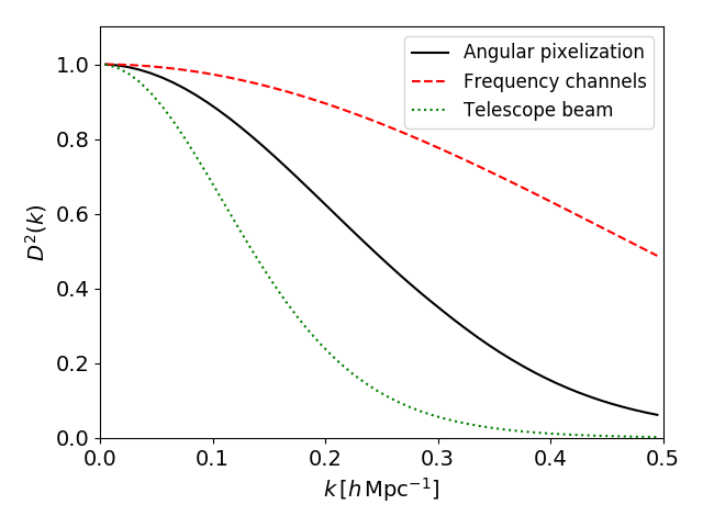
   Figure 1: The damping factor $D^{2}(\textbf{{k}})$ defined by Equation 28 for the simulation tests described in Section 4. We show cases corresponding to the angular pixelization (black solid line) where $(k_{\perp}=k,k_{\parallel}=0)$, the radial frequency channels (red dashed line) where $(k_{\perp}=0,k_{\parallel}=k)$ and the telescope beam (dotted green line) where $(k_{\perp}=k,k_{\parallel}=0)$.

4. We convolved the damped, model power spectra with the window function of the survey cones, $P(\textbf{{k}})\rightarrow P\star|W_{\rm cone}|^{2}$.

5. To allow for the discretization onto the FFT grid, we summed the resulting power spectra over modes $\textbf{{k}}_{\textbf{{n}}}=\textbf{{k}}+2k_{N}\textbf{{n}}$ using Equation 53, taking a $3^{3}$ grid of $\textbf{{n}}=\{-1,0,1\}$.

6. We averaged the model power spectra in the same Fourier bins as the measurements.

The auto- and cross-power spectrum multipole measurements and models for this test case, along with the residuals, are displayed in Figure 2. There is good general agreement between the models and mock observations. The most significant deviation occurs for the monopole of the intensity power spectrum $P_{TT}$, whose measured amplitude lies around $10\%$ below the model. We attribute this offset to the approximations implemented when deriving the damping of the model due to spherical pixelization, as described in Section 2.4. The $P_{gT}$ monopole and $P_{TT}$ quadrupole also show some deviations for scales $k>0.2\,h$ Mpc^-1. Excepting the $P_{TT}$ monopole, all statistics and multipoles produce a satisfactory value of the $\chi^{2}$ statistic with $\chi^{2}/{\rm dof}\sim 1$ for scales $k<0.2\,h$ Mpc^-1.

Current cross-correlation analyses of radio intensity mapping and galaxy surveys have produced $\sim 3$-$\sigma$ detections of the cross-power spectrum amplitude, and corresponding constraints on the neutral hydrogen density at intermediate redshifts (Chang et al., 2010; Masui et al., 2013; Wolz et al., 2017; Anderson et al., 2018). Analysis of the auto-power spectrum of intensity maps is currently severely limited by imperfect foreground subtraction. Hence, we conclude that our model is likely to remain sufficient for the analysis of near-future intensity mapping datasets, which will focus on cross-correlation measurements.

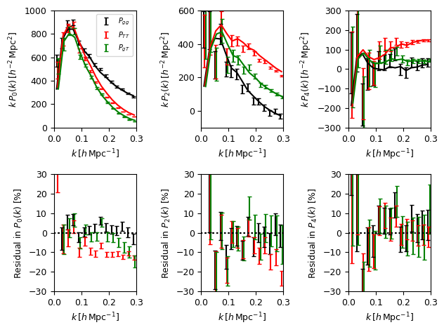
Figure 2: The auto-power spectrum multipoles of the simulated galaxy survey $P_{gg}$ (black error bars) and intensity-mapping survey $P_{TT}$ (red errors), and the cross-power spectrum multipoles $P_{gT}$ (green errors). The left-hand, middle and right-hand upper panels show the monopole ($P_{0}$), quadrupole ($P_{2}$) and hexadecapole ($P_{4}$), respectively, and the solid lines display the computed models in each case. The power spectra are scaled by a factor of $k$ for clarity of presentation. The lower panels display the residual between the measured power spectra and models, expressed as a percentage of the corresponding monopole power in each case.

5 Summary

In this paper we have provided a general framework connecting the measured 2-point auto- and cross-correlations of fluctuation fields to their underlying cosmological power spectra, in the presence of a variety of observational effects. Our framework can be applied to the analysis of galaxy spectroscopic redshift surveys, datasets with accurate photometric redshifts, radio intensity-mapping surveys, or other 3D cosmological maps.

The observational effects we considered are the variation with position of the background level of the field, measurement noise, the smoothing and discretization of the field, and the changing line-of-sight direction. We extended previous literature by deriving that if a field is smoothed by a position-dependent kernel, $B(\textbf{{s}},\textbf{{x}})$, where s is the kernel separation with respect to position x, then the power spectrum is damped by the volume-average of the Fourier transform of the kernel at each position, $\frac{1}{V}\int d^{3}\textbf{{x}}\,|\tilde{B}(\textbf{{k}},\textbf{{x}})|^{2}$, under the approximation that $\tilde{B}(\textbf{{k}},\textbf{{x}})$ varies slowly with x. We applied this result to the cases of averaging a field in irregular cells, applying noise in these cells, a telescope beam, redshift errors, and binning data in frequency channels and angular pixels.

We reviewed the direct estimators of the auto- and cross-power spectra, their multipoles, and the variance in these statistics. We extended the results of Feldman et al. (1994) to present optimal weights for measuring the auto- and cross-power spectra of general cosmological fluctuation fields, with application to galaxy surveys and intensity maps. FKP weights for individual tracers do not in general provide the optimal weights when measuring the cross-power spectrum.

We validated our model by comparison with the power spectrum multipoles of a mock galaxy and intensity-mapping dataset drawn from an N-body simulation, including several of these observational effects. The intensity mapping component of this simulated dataset lies roughly an order of magnitude in precision beyond current observations. The model is effective in reproducing the measured statistics, excepting a $\sim 10\%$ residual in the monopole of the intensity auto-power spectrum, $P_{TT}$. However, given that current analyses of $P_{TT}$ are limited by imperfect foreground subtraction, our model is likely to remain sufficient for the analysis of near-future intensity-mapping datasets. We note that a number of other observational effects, such as fibre collisions, selection function systematics, radio foregrounds and photometric redshift outliers, are not considered in this study but may be relevant for the analysis of real data.

We hope that this study has provided a set of recipes and derivations which will be useful for modelling and studying the Fourier-space statistics of cosmological fluctuation fields in observed and simulated datasets. Accompanying power spectrum code for producing our mock dataset and evaluating the measurements and models is available at https://github.com/cblakeastro/intensitypower.

References

• Anderson et al. (2018) Anderson C. J., et al., 2018, MNRAS, 476, 3382
• Astropy Collaboration et al. (2013) Astropy Collaboration et al., 2013, A&A, 558, A33
• Bandura et al. (2014) Bandura K., et al., 2014, in Ground-based and Airborne Telescopes V. p. 914522 (arXiv:1406.2288), doi:10.1117/12.2054950
• Beutler et al. (2014) Beutler F., et al., 2014, MNRAS, 443, 1065
• Beutler et al. (2017) Beutler F., et al., 2017, MNRAS, 466, 2242
• Bianchi et al. (2015) Bianchi D., Gil-Marín H., Ruggeri R., Percival W. J., 2015, MNRAS, 453, L11
• Blake et al. (2013) Blake C., et al., 2013, MNRAS, 436, 3089
• Blake et al. (2018) Blake C., Carter P., Koda J., 2018, MNRAS, 479, 5168
• Castorina & White (2018) Castorina E., White M., 2018, MNRAS, 476, 4403
• Chang et al. (2010) Chang T.-C., Pen U.-L., Bandura K., Peterson J. B., 2010, Nature, 466, 463