Pyrochlore U(1) spin liquid of mixed symmetry enrichments in magnetic fields

Abstract

We point out the experimental relevance and the detection scheme of symmetry enriched U(1) quantum spin liquids (QSLs) outside the perturbative spin-ice regime. Recent experiments on Ce-based pyrochlore QSL materials suggest that the candidate QSL may not be proximate to the well-known spin ice regime, and thus differs fundamentally from other pyrochlore QSL materials. We consider the possibility of the $\pi$-flux U(1) QSL favored by frustrated transverse exchange interactions rather than the usual quantum spin ice. It was previously suggested that both dipolar U(1) QSL and octupolar U(1) QSL can be realized for the generic spin model for the dipole-octupole doublets of the Ce³⁺ local moments on the pyrochlore magnets Ce₂Sn₂O₇ and Ce₂Zr₂O₇. We explain and predict the experimental signatures especially the magnetic field response of the octupolar $\pi$-flux U(1) QSL. Fundamentally, this remarkable state is a mixture of symmetry enrichments from point group symmetry and from translational symmetry. We discuss the relevant experiments for pyrochlore U(1) QSLs and further provide some insights to the pyrochlore Heisenberg model.

I Introduction

Symmetry is the key that underlies the traditional Landau’s paradigm of many-body phases and phase transitions. It is almost so in the classification and understanding of topological and exotic phases of quantum matter Wen (2007). In last decade or so, a tremendous progress has been made theoretically to classify various symmetry enriched topological phases, where symmetry creates much more topological phases Wen (2002); Essin and Hermele (2013); Mesaros and Ran (2013); Levin and Wen (2005); Qi et al. (2019); Chen and Hermele (2016); Chen (2017a). These symmetry enriched topological phases are described by the same topological quantum field theory, but they are distinct by the realization of symmetries for example on the fractionalized excitations. These beautiful theories so far do not have strong experimental connections. It is thus of a great interest to find an experimental relevance and establish the connection.

In last decade or so, various quantum spin liquid (QSL) candidate materials have been proposed, and the rare-earth pyrochlore magnets comprise an important and large family of materials Molavian et al. (2007); Ross et al. (2011); Benton et al. (2012); Fritsch et al. (2014); Arpino et al. (2017); MacLaughlin et al. (2015); Wen et al. (2017); Applegate et al. (2012); Benton (2018, 2016); Dunsiger et al. (2011); Lhotel et al. (2014); Chang et al. (2014); Yasui et al. (2003); Sibille et al. (2018); Hao et al. (2014); Wan and Tchernyshyov (2012); Onoda and Tanaka (2010); Lantagne-Hurtubise et al. (2017); Khemani et al. (2012); Udagawa and Moessner (2018) in these proposals. In these materials, the rare-earth ions carry spin-orbital-entangled effective spin-1/2 local moments that interact with highly anisotropic superexchange interactions Curnoe (2008); Ross et al. (2011); Onoda and Tanaka (2011); Onoda (2011); Huang et al. (2014) Due to the proximity to the classical spin ice regime where the classical Ising interaction dominates, many pyrochlore materials develop a spin ice type of Pauling entropy plateau at low but finite temperatures Castelnovo1 et al. (2008); Castelnovo et al. (2011); Bramwell and Gingras (2001); Gingras and McClarty (2014); Gardner et al. (2010); Isakov et al. (2005); Kaiser et al. (2015); Molavian et al. (2007). Introducing quantum fluctuations and/or perturbations to the extensively degenerate spin ice manifold could then convert the system into a QSL state, and this state is often quoted as quantum spin ice U(1) QSL or pyrochlore ice U(1) QSL Hermele et al. (2004); Huse et al. (2003); Motrunich and Senthil (2005); Molavian et al. (2007); Gingras and McClarty (2014); Ross et al. (2011); Savary and Balents (2012). Is the proximity to the spin ice regime necessary to produce a U(1) QSL? In our opinion, this condition was merely a theoretical convenience to access the interesting and exotic state in early theoretical works Hermele et al. (2004); Savary and Balents (2012). It is now established that, the pyrochlore U(1) QSL is much more robust in the so-called frustrated regime where the spinon experiences an emergent background $\pi$ flux Lee et al. (2012); Chen (2017b); Taillefumier et al. (2017); Benton et al. (2018). Since this $\pi$-flux U(1) QSL is expected to extend much beyond the perturbative spin ice regime Lee et al. (2012), it is natural to expect that the proximity to the spin ice regime is not quite necessary to obtain the pyrochlore U(1) QSL. We refer the U(1) QSL in this regime as non-spin-ice pyrochlore U(1) QSL or simply as pyrochlore U(1) QSL instead of pyrochlore spin ice U(1) QSL.

In the actual experiments on the Ce-based pyrochlore QSL materials (in particular, Ce₂Zr₂O₇) Gao et al. (2019), there does not exist the spin ice type of Pauling entropy plateau down to very low temperatures while the magnetic entropy is almost completely exhausted. This is a clear indication that the system is not in the spin ice regime. Another interesting aspect is that the Ce³⁺ local moment in both Ce₂Sn₂O₇ Sibille et al. (2015, 2019); Lovesey and van der Laan (2020) and Ce₂Zr₂O₇ is a dipole-octupole doublet Huang et al. (2014); Li and Chen (2017); Li et al. (2016). It is thus natural for us to consider the possibility of pyrochlore U(1) QSL beyond the spin ice regime with the dipole-octupole doublets. It was previously suggested that, the anisotropic interaction between the dipole-octupole doublets on the pyrochlore lattice could stabilize two symmetry enriched U(1) QSLs, i.e. dipolar U(1) QSL and octupolar U(1) QSL Huang et al. (2014); Li and Chen (2017). The major distinction between these two U(1) QSLs arises from the transformation of emergent electric field under the point group symmetry operation, i.e., the emergent electric field in the dipolar U(1) QSL transforms as the magnetic dipole moment while the emergent electric field in the octupolar U(1) QSL transforms as the magnetic octupole moment. On top of this point group symmetry enrichment, there is an additional translational symmetry enrichment where the spinon could experience a background $\pi$ flux or $0$ flux in the distinct enrichments. It was shown that, Lee et al. (2012) the $\pi$ flux state (labelled as U(1)_π QSL) extends much beyond the perturbative ice regime. Therefore, it is reasonable to associate the non-spin-ice pyrochlore QSL with the U(1)_π QSL. The 0 flux state (labelled as U(1)₀ QSL) has been studied extensively in the previous literature Savary and Balents (2012); Lee et al. (2012); Huang et al. (2014). For the dipole-octupole doublets, the octupolar U(1)₀ QSL has been studied by us in a previous work Li and Chen (2017), and in the current work, we will mostly focus on the octupolar U(1)_π QSL and explore its physical properties.

The octupolar U(1)_π QSL is the quantum phase that most clearly reflects the interplay between the multipolar nature of the local moments and emergent exotic properties of the U(1) QSL. The strong frustrated interaction between the octupolar components is the precondition for realizing the octupolar U(1)_π QSL. In terms of the emergent degrees of freedom for the octupolar U(1)_π QSL, the octupole component is the emergent electric field whose correlation contains both the gapess U(1) gauge photon and the gapped “magnetic monopoles”. These magnetic octupole components, however, do not couple with the external magnetic field and the neutron spin at the linear order. Thus, they are hidden from the conventional measurements. What is visible is the spinon sector. The external magnetic field couples linearly with the dipole component that does not commute with the octupole component or the emergent electric field. Thus it is observed that Li and Chen (2017), the external magnetic field couples with the spinon-antispinon pair and modifies the spinon dispersion. For the octupolar U(1)_π QSL, the spinon continuum has a spectral periodicity enhancement due to the background $\pi$ flux. We specifically study the experimental signatures of the octupolar U(1)_π QSL for the frustrated non-spin-ice regime and explore the spinon continuum and the magnetic excitations under the magnetic fields.

The remaining parts of the paper are organized as follows. In Sec. II, we introduce the model for the dipole-octupole doublets on the pyrochlore lattice and emphasize the unique coupling to magnetic fields. In Sec. III, we explain the connection between the microscopic degrees of freedom and the emergent degrees of freedom in the octupolar U(1)_π QSL. In Sec. IV, we explore the impact of the external magnetic field on the spinon continuum in the octupolar U(1)_π QSL. In Sec. V, we analyze the spin-wave spectrum in the regime with strong magnetic fields. Finally in Sec. VI, we discuss some experimental relevance and the related theoretical questions.

II Effective spin model

We start with the generic effective spin model for the dipole-octupole doublets on the pyrochlore lattice. The model was derived in Ref. Huang et al., 2014 and is known as the XYZ model Huang et al. (2014); Li and Chen (2017); Li et al. (2016),

$$H = \sum_{\langle ij\rangle}J_{z}S^{z}_{i}S^{z}_{j}+J_{x}S^{x}_{i}S^{x}_{j}+J_{y}S^{y}_{i}S^{y}_{j}$$ (1)

$$+J_{xz}(S^{x}_{i}S^{z}_{j}+S^{z}_{i}S^{x}_{j})-h\sum_{i}(\hat{n}\cdot\hat{z}_{i})S_{i}^{z},$$

where microscopically $S^{x}$ and $S^{y}$ are magnetic octupole moments while $S^{z}$ is a magnetic dipole moment. From the symmetry analysis, $S^{x}$ and $S^{z}$ transform identically under the point group symmetry. Thus, $S^{x}$ is sometimes referred as the magnetic dipole moment Huang et al. (2014). We have also introduced the Zeeman coupling that only acts on the magnetic dipole moment $S^{z}$, and $\hat{n}$ is the field direction and $\hat{z}_{i}$ defines the local $z$ direction of each sublattice (see Appendix A for definition of these conventions). Only the nearest-neighbor interaction is considered here, which is expected to be reasonable for the localized $4f$ electrons. The XYZ form is obtained by applying a rotation around the $y$-direction by an angle $\theta$ to eliminate the $J_{xz}$ term; the resulting Hamiltonian reads

$$H_{\text{XYZ}} = \sum_{\langle ij\rangle}\tilde{J}_{z}\tilde{S}^{z}_{i}\tilde{S}^{z}_{j}+\tilde{J}_{x}\tilde{S}^{x}_{i}\tilde{S}^{x}_{j}+\tilde{J}_{y}\tilde{S}^{y}_{i}\tilde{S}^{y}_{j}$$ (2)

$$-h\sum_{i}(\hat{n}\cdot\hat{z}_{i})(\cos\theta\tilde{S}_{i}^{z}+\sin\theta\tilde{S}_{i}^{x}),$$

where $\tilde{S}_{i}^{x,z}$ are related to ${S}_{i}^{x,z}$ by the $\theta$-rotation, and ${\tilde{S}^{y}\equiv S^{y}}$. In the phase diagram of $H_{\text{XYZ}}$ without the magnetic field, the system supports three disconnected U(1) QSLs Li and Chen (2017); Huang et al. (2014). When $\tilde{J}_{z}$ ($\tilde{J}_{y}$) is antiferromagnetic and dominant while the remaining two couplings are not large enough to drive a magnetic order, the ground state is a dipolar (an octupolar) U(1) QSL. In the case when $\tilde{J}_{x}$ is antiferromagnetic and large, the relevant U(1) QSL is regarded as a dipolar U(1) QSL and shares the same universal and qualitatively similar physics with the dipolar U(1) QSL because $\tilde{S}^{x}$ and $\tilde{S}^{z}$ transform identically under the point group symmetry. The dipolar U(1) QSL and the octupolar U(1) QSL are symmetry enriched U(1) QSLs and are enriched by the point group symmetry.

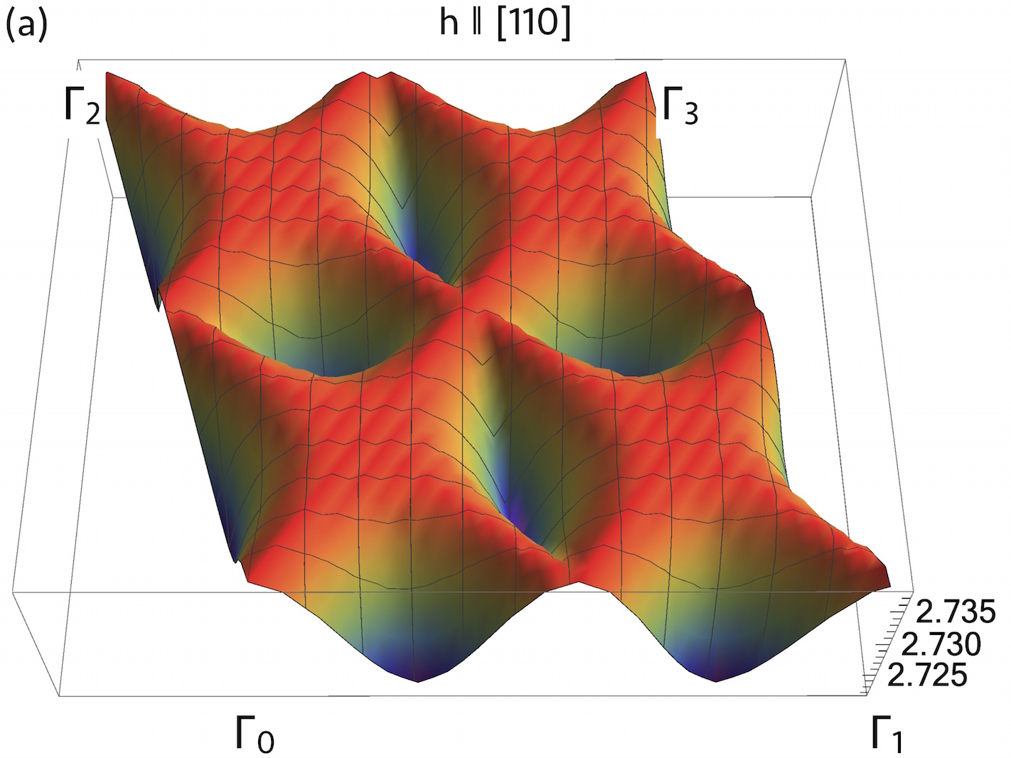
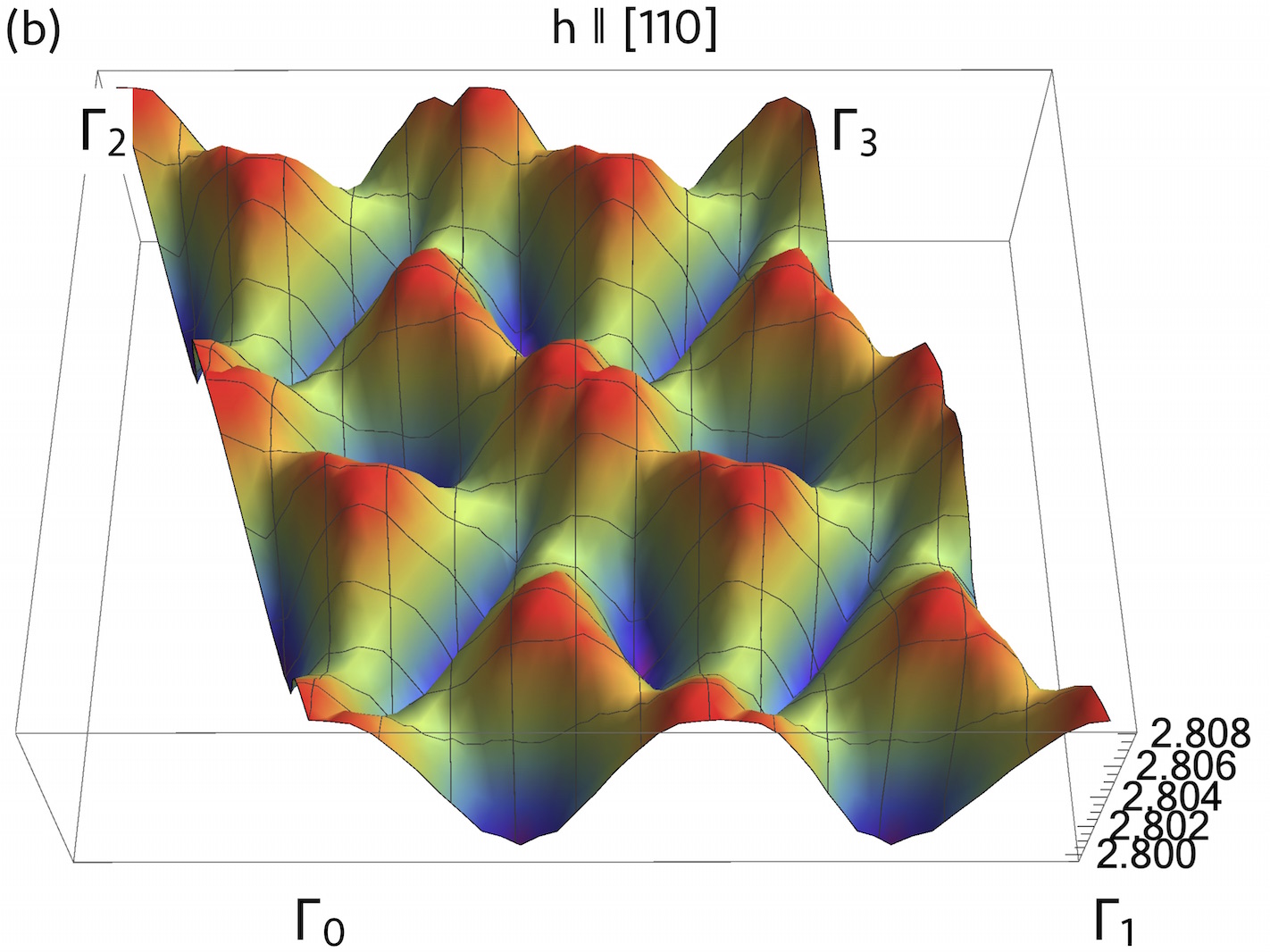
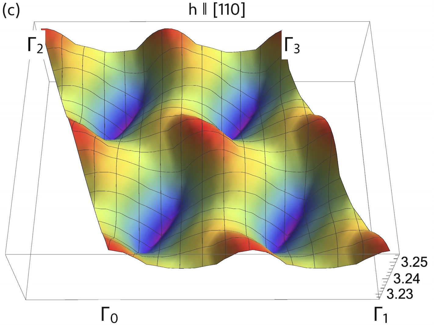
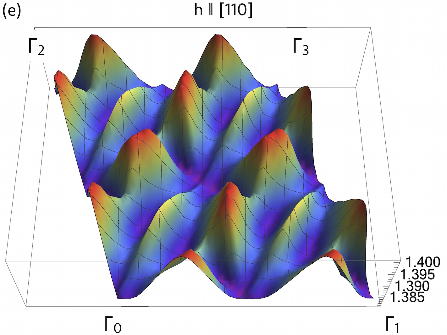
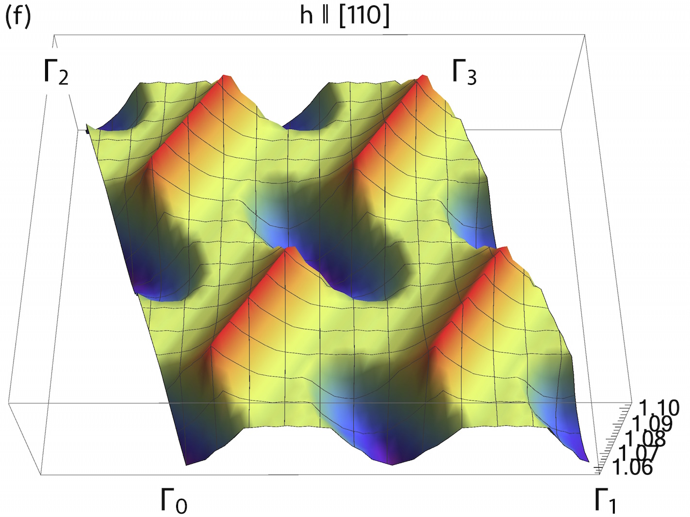
Figure 1: (Color online.) The upper and lower excitation edges of the two-spinon continuum in the octupolar U(1)_π QSL, for the magnetic fields along the [110] direction. We fix ${J_{\pm}^{y}=-0.33J_{y}},{J_{\pm\pm}^{y}}=0,{\theta=0}$, and take ${h=0}$ in (a, d), ${h=0.2J_{y}}$ in (b, e), and ${h=1.0J_{y}}$ in (c, f). The energy unit is set to $J_{y}$. Here, the $\Gamma$ points represent the Brillouin zone centers and differ by the reciprocal lattice vectors with ${\Gamma_{0}\Gamma_{1}=2\pi(-1,1,1)}$ and ${\Gamma_{0}\Gamma_{2}=2\pi(1,-1,1)}$.

III Octupolar U(1)_π QSL

Since the experiments suggest that Ce₂Zr₂O₇ is not in the spin ice regime Gao et al. (2019), we would like to understand this from the physical properties of both dipolar and octupolar U(1) QSLs in the non-spin-ice regime. From the previous argument and early results Lee et al. (2012), the non-spin-ice regime for a XXZ model would be in the frustrated regime with a frustrated transverse exchange interaction and support the U(1) QSL with $\pi$ flux for spinons.

The XYZ model with zero magnetic field can be rewritten with two different but equivalent forms below,

$${H}_{z} = \sum_{\langle ij\rangle}\tilde{J_{z}}\sigma^{z}_{i}\sigma^{z}_{j}-J_{\pm}^{z}(\sigma^{+}_{i}\sigma^{-}_{j}+\sigma^{-}_{i}\sigma^{+}_{j})+J_{\pm\pm}^{z}(\sigma^{+}_{i}\sigma^{+}_{j}+\sigma^{-}_{i}\sigma^{-}_{j}),$$ (3)

$${H}_{y} = \sum_{\langle ij\rangle}\tilde{J_{y}}\tau^{y}_{i}\tau^{y}_{j}-J_{\pm}^{y}({\tau}^{+}_{i}{\tau}^{-}_{j}+{\tau}^{-}_{i}{\tau}^{+}_{j})+J_{\pm\pm}^{y}({\tau}^{+}_{i}{\tau}^{+}_{j}+{\tau}^{-}_{i}{\tau}^{-}_{j}),$$ (4)

where we have

$$\sigma_{i}^{z}\equiv\tilde{S}_{i}^{z},\quad{\sigma^{\pm}_{i}\equiv\tilde{S}^{x}_{i}\pm i\tilde{S}^{y}_{i}}$$ (5)

$$\tau^{y}\equiv\tilde{S}_{i}^{y},\quad{\tau^{\pm}_{i}\equiv\tilde{S}^{z}_{i}\pm i\tilde{S}^{x}_{i}}$$ (6)

and the couplings $(J_{\pm}^{z},J_{\pm\pm}^{z})$ and $(J_{\pm}^{y},J_{\pm\pm}^{y})$ can be read off from the expansion the above two Hamiltonians into the original form. For convenience, we focus on the regime where the ground state of $H_{z}$ ($H_{y}$) is the dipolar (octupolar) U(1) QSL, i.e. when $\tilde{J}_{z}$ ($\tilde{J}_{y}$) is antiferromagnetic and dominant. It is known that, as long as ${J_{\pm}^{z}>0}$ (${J_{\pm}^{y}>0}$), the model for either sign of $J_{\pm\pm}^{z}$ ($J_{\pm\pm}^{y}$) does not have a fermion sign problem for quantum Monte carlo simulation Huang et al. (2014). In this unfrustrated regime, numerics shows that the system has the classical spin ice phenomena such as the Pauling entropy plateau at low and finite temperatures even when the system is located in the QSL phase at zero temperature Huang et al. (2018). It means that the frustrated regime ${J_{\pm}^{z}<0}$ (${J_{\pm}^{y}<0}$) should carry the QSL physics for the Ce-based pyrochlore magnets. Since the frustrated regime for the U(1) QSL generates an emergent $\pi$-flux for the spinons, it is then natural to understand the physical properties of the dipolar and octupolar U(1)_π QSLs. It is interesting to note that the $\pi$ flux for the spinons is a signature of the symmetry enrichments in the lattice translation of the spinon sector. This is a translational symmetry enrichment on top of the point group symmetry enrichments. Due to the $\pi$ flux, we expect the spinon continuum to develop an enhanced spectral periodicity in the reciprocal space with a folded Brillouin zone Chen (2017b); Essin and Hermele (2014). Although certain generic properties may be established from the model level, there is still a gap to a quantitative connection to the actual physical observables of the dipole-octupole doublets.

To make connection with the experiments, it is important to notice that only $S^{z}$ in Eq. (1) is magnetic Huang et al. (2014); Li and Chen (2017); Li et al. (2016), and only $S^{z}$-$S^{z}$ correlation is measurable in a neutron scattering experiment. From Eq. (2), ${S^{z}_{i}=\cos\theta\sigma_{i}^{z}+\sin\theta\sigma_{i}^{x}}$. Thus, the inelastic neutron scattering experiment would measure both $\sigma^{z}$-$\sigma^{z}$ and $\sigma^{x}$-$\sigma^{x}$ correlators. For the dipolar U(1)_π QSL of $H_{z}$ with a large and antiferromagnetic $\tilde{J}_{z}$ (for the dipolar U(1)_π QSL with a large and antiferromagnetic $\tilde{J}_{x}$), the spinon continuum is contained in the $\sigma^{x}$-$\sigma^{x}$ ($\sigma^{z}$-$\sigma^{z}$) correlator, and the “magnetic monopole” continuum and the gauge photon are contained in the $\sigma^{z}$-$\sigma^{z}$ ($\sigma^{x}$-$\sigma^{x}$) correlator. The inclusion of the “magnetic monopole” continuum was understood quite recently Chen (2017). Due to the background $\pi$ flux for the spinons in the dipolar U(1)_π QSL, the spinon continuum develops an enhanced spectral periodicity with a folded Brillouin zone Chen (2017, 2017b); Lee et al. (2012). For the “magnetic monopoles”, the continuum should always have an enhanced spectral periodicity with a folded Brillouin zone due to the effective spin-1/2 nature of the local moment Chen (2017, 2017b, 2016). As for the octupolar U(1)_π QSL, because $\tau^{y}$ is not directly measurable, the ${S}^{z}$-${S}^{z}$ correlator only detects the gapped spinon continuum, and the continuum has an enhanced spectral periodicity Li and Chen (2017); Chen (2017, 2017b).

IV Evolution of spinon continuum under magnetic fields for octupolar U(1)_π QSL

To access the ground state and illustrate the emergent U(1) gauge structure and the physical properties of the XYZ spin model, we implement the mapping introduced in Refs. Savary and Balents, 2012; Lee et al., 2012 of the spin model to an Abelian-Higgs model with the compact U(1) gauge field and the bosonic spinon matter. Focusing on the octupolar U(1) QSL regime (when $\tilde{J}_{y}$ is positive and dominant in Eq. (4)), we express the spin operators as

$${\tau^{y}_{{\textbf{r}},{\textbf{r}}+{\textbf{e}}_{\mu}}=s^{y}_{{\textbf{r}},{\textbf{r}}+{\textbf{e}}_{\mu}}},\quad{\tau^{+}_{{\textbf{r}},{\textbf{r}}+{\textbf{e}}_{\mu}}=\Phi^{\dagger}_{{\textbf{r}}}s^{+}_{{\textbf{r}},{\textbf{r}}+{\textbf{e}}_{\mu}}\Phi^{\phantom{\dagger}}_{{\textbf{r}}+{\textbf{e}}_{\mu}}},$$ (7)

where r belongs to the I diamond sublattice (our convention is summarized in Appendix A). Here $s^{y}_{{\textbf{r}},{\textbf{r}}^{\prime}}$ is the emergent electric field in the octupolar U(1) QSL phase, $s^{\pm}_{{\textbf{r}},{\textbf{r}}^{\prime}}$ is the gauge string operator ending at sites r and ${\textbf{r}}^{\prime}$, and $\Phi^{\phantom{\dagger}}_{{\textbf{r}}}$ ($\Phi^{\dagger}_{{\textbf{r}}}$) is the spinon annihilation (creation) operator at the diamond lattice site r. The physical Hilbert space is obtained by imposing the following constraints

$$Q_{\textbf{r}}=\eta_{\textbf{r}}\sum_{\mu}s^{y}_{{\textbf{r}},{\textbf{r}}+\eta_{\textbf{r}}{\textbf{e}}_{\mu}},\quad\Phi^{\dagger}_{{\textbf{r}}}\Phi^{\phantom{\dagger}}_{{\textbf{r}}}=1,$$ (8)

where ${\eta_{{\textbf{r}}}=\pm 1}$ for r in sublattice I and II, respectively, and $Q_{{\textbf{r}}}$ is the operator measuring the local gauge charge through the “Gauss law”, and is canonically conjugate to $\Phi_{{\textbf{r}}}$,

$$\left[\Phi^{\phantom{\dagger}}_{{\textbf{r}}},Q_{{\textbf{r}}}\right]=\Phi^{\phantom{\dagger}}_{{\textbf{r}}},\quad\left[\Phi^{\dagger}_{{\textbf{r}}},Q_{{\textbf{r}}}\right]=\Phi^{\dagger}_{{\textbf{r}}}.$$ (9)

Under this mapping the Hamiltonian becomes

$$H_{y} = \frac{\tilde{J}_{y}}{2}\sum_{{\textbf{r}}}Q_{\textbf{r}}^{2}-J_{\pm}^{y}\sum_{\textbf{r}}\sum_{\mu\neq\nu}\left(\Phi^{\dagger}_{{\textbf{r}}+\eta_{\textbf{r}}{\textbf{e}}_{\mu}}\Phi^{\phantom{\dagger}}_{{\textbf{r}}+\eta_{\textbf{r}}{\textbf{e}}_{\nu}}s^{-\eta_{\textbf{r}}}_{{\textbf{r}},{\textbf{r}}+\eta_{\textbf{r}}{\textbf{e}}_{\mu}}s^{+\eta_{\textbf{r}}}_{{\textbf{r}},{\textbf{r}}+\eta_{\textbf{r}}{\textbf{e}}_{\nu}}\right)$$ (10)

$$+\frac{J_{\pm\pm}^{y}}{2}\sum_{\textbf{r}}\sum_{\mu\neq\nu}\left(\Phi^{\dagger}_{{\textbf{r}}}\Phi^{\dagger}_{{\textbf{r}}}\Phi^{\phantom{\dagger}}_{{\textbf{r}}+\eta_{\textbf{r}}{\textbf{e}}_{\mu}}\Phi^{\phantom{\dagger}}_{{\textbf{r}}+\eta_{\textbf{r}}{\textbf{e}}_{\nu}}s^{+\eta_{\textbf{r}}}_{{\textbf{r}},{\textbf{r}}+\eta_{\textbf{r}}{\textbf{e}}_{\mu}}s^{+\eta_{\textbf{r}}}_{{\textbf{r}},{\textbf{r}}+\eta_{\textbf{r}}{\textbf{e}}_{\nu}}+h.c.\right)$$

$$-\frac{h}{4}\sum_{\textbf{r}}\sum_{\mu}\left(\hat{{n}}\cdot\hat{{z}}_{{\textbf{r}}+\eta_{\textbf{r}}{\textbf{e}}_{\mu}/2}\right)\left[\cos\theta\left(\Phi^{\dagger}_{{\textbf{r}}}\Phi^{\phantom{\dagger}}_{{\textbf{r}}+\eta_{\textbf{r}}{\textbf{e}}_{\mu}}s^{+\eta_{\textbf{r}}}_{{\textbf{r}},{\textbf{r}}+\eta_{\textbf{r}}{\textbf{e}}_{\mu}}+h.c.\right)-i\sin\theta\left(\Phi^{\dagger}_{{\textbf{r}}}\Phi^{\phantom{\dagger}}_{{\textbf{r}}+\eta_{\textbf{r}}{\textbf{e}}_{\mu}}s^{+\eta_{\textbf{r}}}_{{\textbf{r}},{\textbf{r}}+\eta_{\textbf{r}}{\textbf{e}}_{\mu}}-h.c.\right)\right].$$

Within the U(1)_π QSL regime, we choose a gauge to take care of the background $\pi$-flux Lee et al. (2012); Chen (2017b), such that the spinons hop on the diamond lattice with modulated signs of hoppings (see Appendix A). In the absence of the field, the spinon continuum, that is measurable via an inelastic neutron scattering measurement in the octupolar U(1)_π QSL, shows a spectral periodicity enhancement with a folded Brillouin zone. As we calculate explicitly and show in the left panel of Fig. 1, both the upper and lower excitation edges of the two-spinon continuum develop the spectral periodicity enhancement. Another advantage of the octupolar U(1) QSL is to allow the external magnetic field to tune the spinon dispersion directly even in the presence of the background $\pi$ flux.

The external magnetic field, that couples to $S^{z}$ or equivalently couples to the spinon matters, modifies the spinon band structures. This modification can then be directly measured by the inelastic neutron scattering probe. This provides an interesting example to manipulate or control the emergent fractionalized spinon degrees of freedom with external means that is the external magnetic field here. More importantly, such a manipulability could be recorded and tested experimentally. We apply the fields along three high symmetry directions, i.e. [001], [110] and [111] crystallographic directions. In the central panel and the right panel of Fig. 1, we plot the upper and lower excitation edges of the spinon continuum under two different magnetic fields along the [110] direction. Because the weak magnetic field does not revise the background $\pi$ flux, the spinon continuum in these plots continues to develop an enhanced spectral periodicity with a folded Brillouin zone. This important topological property remains to be the distinct feature to be examined even in the presence of the magnetic field. The detailed calculation scheme and the results for the fields along the [001] and [111] directions are displayed in Appendix B and Appendix C. Despite the application of the magnetic fields, the enhanced spectral periodicity preserves, and the magnetic field also generates non-universal features such as the rich wiggles in the spectra.

The above calculation is based on the assertion that the 3D U(1) QSL is stable against the perturbation from the weak magnetic fields. What happens if the field becomes strong? To address this question, we notice that there is a (hidden) competition between the transverse spin exchange interaction and the magnetic field. Our observation is as follows. The strong magnetic field would simply favor an uniform polarized state that preserves the lattice translations, while the simple spinon condensation of the U(1)_π QSL would favor a state that breaks the lattice translational symmetry Chen (2017b). This frustration could enhance the stability of U(1)_π QSL against the external magnetic field. The stability of U(1)_π QSL against exchange interactions and other competing orders has been previously established in Ref. Lee et al., 2012 and Ref. Benton et al., 2018, respectively. This might also be the reason for the more stability of the antiferromagnetic Kitaev QSL in the magnetic field over the ferromagnetic one Zhu et al. (2018). Perturbatively, the magnetic field favors a zero-flux state. One may wonder if the field can drive a phase transition between two symmetry enriched U(1) QSLs, i.e., from U(1)_π to U(1)₀ QSLs, and then from U(1)₀ QSL to the spinon condensed state, or a direct first order transition from U(1)_π QSL to the polarized state, or the field first drives a spinon condensation by breaking the lattice translation and then restores the lattice transition by entering a polarized phase via a first order transition. This may be examined numerically or experimentally.

V Magnetic excitations in the strong field regime

As the external magnetic field is further increased, the system will eventually enter a polarized state. For the fully or nearly polarized state, the spins (or the local $z$ components) are aligned along the preferred direction according to the external magnetic field. Since the transverse spin components that create the coherent spin excitations are the octupolar moments, the neutron spin does not couple linearly with the transverse spin component and thus the inelastic neutron scattering signal would be suppressed. However, there can still be residual intensity for the nearly polarized state due to the crossing coupling $J_{xz}(S_{i}^{x}S_{j}^{z}+S_{i}^{z}S_{j}^{x})$. This can be understood as follows. Although the magnetic field polarizes the $S^{z}$ components directly, the finite $S^{z}$ would further induce a finite $S^{x}$ through the crossing coupling. As a result, the $S^{z}$ operator could create coherent magnetic excitations by flipping $S^{x}$ components.

The distinction between the dipolar U(1) QSL and the octupolar U(1) QSL not only appears in the qualitative behaviors under the weak magnetic fields or by the neutron scattering measurements, but also shows up in the magnetic excitations when the QSL state is replaced by the polarized states in the strong magnetic fields. The former has been explained in the previous sections. The latter can be simply understood as follows. We directly compare the dipolar U(1) QSL with a dominant $\tilde{J}_{z}$ with the octupolar U(1) QSL with a dominant $\tilde{J}_{y}$. Regardless of which U(1) QSL the system is located in, it is always the transverse spin component that flips the $S^{z}$ components and generates the spin wave excitation in the polarized state. As the transverse couplings for two distinct U(1) QSLs are very different compared to the dominant interactions, it is meaningful to explore quantitatively the spin wave dispersion under different magnetic fields in different symmetry enriched U(1) QSLs with distinct parameter regimes, and this information would in principle be able to distinguish which U(1) QSL the polarized state may be originated from.

To illustrate the above thoughts, we proceed to calculate the spin wave dispersions for the parameter choices of the dipolar U(1) QSL and the octupolar U(1) QSL, respectively. In practice, one obtains the spin wave spectra from the neutron scattering measurement by applying magnetic fields to polarize the spin and then extract the couplings. Since the experiments are not available yet, we choose the representative parameters for the dipolar U(1) QSL and the octupolar U(1) QSL, and perform our spin wave analysis. To carry out the actual calculation, we invoke the well-known Holstein-Primakoff spin wave theory to expand the spin operator. We first consider the application of the magnetic field along the [111] direction. In the strong field limit, the spin configuration would simply be a “3-in 1-out” state. For our parameter choices that are given in Fig. 2 and Fig. 3, it is legitimate to express the spin operators of the 0-th sublattice as,

$$S_{i}^{+} = b_{i},\quad S_{i}^{-}=b_{i}^{\dagger},$$ (11)

$$S_{i}^{z} = {1}/{2}-b_{i}^{\dagger}b_{i},$$ (12)

and for the remaining three sublattices, we have

$$S_{i}^{+} = b_{i}^{\dagger},\quad S_{i}^{-}=b_{i},$$ (13)

$$S_{i}^{z} = -{1}/{2}+b_{i}^{\dagger}b_{i}.$$ (14)

After substituting $S_{i}$ in Eq. (1) with the bosonic creation (annihilation) operators $b_{i}^{\dagger}$ ($b_{i}$) and then performing the Fourier transformation

$$b_{i}=\frac{1}{\sqrt{L}}\sum_{\bm{k}\in\text{B.Z.}}b_{s}(\bm{k})e^{i\bm{k}\cdot\bm{r}_{l}},$$ (15)

where $\bm{r}_{l}$ is the position vector of unit cell containing magnetic ion $i$ and $s$ refers to the corresponding sublattice index, the XYZ model Hamiltonian under the magnetic field can be recast in terms of boson bilinears as

$$H_{sw}=\sum_{\bm{k}\in\text{B.Z.}}\bm{b}^{\dagger}(\bm{k})h(\bm{k})\bm{b}(\bm{k})+H_{\text{Zeeman}}(\bm{k}).$$ (16)

Here, $\bm{b}(\bm{k})$ is a set of bosonic operator basis $\bm{b}(\bm{\bm{k}})=[b_{0}(\bm{k}),\ldots,b_{3}(\bm{k}),b_{0}^{\dagger}(-\bm{k})\ldots,b_{3}^{\dagger}(-\bm{k})]^{T}$ and $h(\bm{k})$ is a $8\times 8$ Hermitian matrix that can be written in the block form as

$$h(\bm{k})=\begin{pmatrix}A(\bm{k})&B(\bm{k})\\ B^{\dagger}(\bm{k})&\bar{A}(-\bm{k})\end{pmatrix}+E_{\text{cl}},$$ (17)

where $E_{\text{cl}}$ is the classical ground state energy. The matrix elements $A(\bm{k})$ and $B(\bm{k})$ are defined as

$$A(\bm{k})=\begin{pmatrix}\frac{3}{2}J_{z}&\frac{J_{x}-J_{y}}{8}\big{[}e^{-\frac{i}{2}(k_{y}+k_{z})}+1\big{]}&\frac{J_{x}-J_{y}}{8}\big{[}e^{-\frac{i}{2}(k_{x}+k_{z})}+1\big{]}&\frac{J_{x}-J_{y}}{8}\big{[}e^{-\frac{i}{2}(k_{x}+k_{y})}+1\big{]}\\ \frac{J_{x}-J_{y}}{8}\big{[}e^{\frac{i}{2}(k_{y}+k_{z})}+1\big{]}&-\frac{1}{2}J_{z}&\frac{J_{x}+J_{y}}{8}\big{[}e^{\frac{i}{2}(k_{y}-k_{x})}+1\big{]}&\frac{J_{x}+J_{y}}{8}\big{[}e^{\frac{i}{2}(k_{z}-k_{x})}+1\big{]}\\ \frac{J_{x}-J_{y}}{8}\big{[}e^{\frac{i}{2}(k_{x}+k_{z})}+1\big{]}&\frac{J_{x}+J_{y}}{8}\big{[}e^{\frac{i}{2}(k_{x}-k_{y})}+1\big{]}&-\frac{1}{2}J_{z}&\frac{J_{x}+J_{y}}{8}\big{[}e^{\frac{i}{2}(k_{z}-k_{y})}+1\big{]}\\ \frac{J_{x}-J_{y}}{8}\big{[}e^{\frac{i}{2}(k_{x}+k_{y})}+1\big{]}&\frac{J_{x}-J_{y}}{8}\big{[}e^{\frac{i}{2}(k_{x}-k_{z})}+1\big{]}&\frac{J_{x}-J_{y}}{8}\big{[}e^{\frac{i}{2}(k_{y}-k_{z})}+1\big{]}&-\frac{1}{2}J_{z}\end{pmatrix}$$ (18)

and

$$B(\bm{k})=\begin{pmatrix}0&\frac{J_{x}+J_{y}}{8}\big{[}e^{-\frac{i}{2}(k_{y}+k_{z})}+1\big{]}&\frac{J_{x}+J_{y}}{8}\big{[}e^{-\frac{i}{2}(k_{x}+k_{z})}+1\big{]}&\frac{J_{x}+J_{y}}{8}\big{[}e^{-\frac{i}{2}(k_{x}+k_{y})}+1\big{]}\\ \frac{J_{x}+J_{y}}{8}\big{[}e^{\frac{i}{2}(k_{y}+k_{z})}+1\big{]}&0&\frac{J_{x}-J_{y}}{8}\big{[}e^{\frac{i}{2}(k_{y}-k_{x})}+1\big{]}&\frac{J_{x}-J_{y}}{8}\big{[}e^{\frac{i}{2}(k_{z}-k_{x})}+1\big{]}\\ \frac{J_{x}+J_{y}}{8}\big{[}e^{\frac{i}{2}(k_{x}+k_{z})}+1\big{]}&\frac{J_{x}-J_{y}}{8}\big{[}e^{\frac{i}{2}(k_{x}-k_{y})}+1\big{]}&0&\frac{J_{x}-J_{y}}{8}\big{[}e^{\frac{i}{2}(k_{z}-k_{y})}+1\big{]}\\ \frac{J_{x}+J_{y}}{8}\big{[}e^{\frac{i}{2}(k_{x}+k_{y})}+1\big{]}&\frac{J_{x}+J_{y}}{8}\big{[}e^{\frac{i}{2}(k_{x}-k_{z})}+1\big{]}&\frac{J_{x}+J_{y}}{8}\big{[}e^{\frac{i}{2}(k_{y}-k_{z})}+1\big{]}&0\end{pmatrix}.$$ (19)

$\bar{A}(\bm{k})$ is the complex conjugate of $A(\bm{k})$.

The Zeeman coupling in this approximation becomes

$$H_{\text{Zeeman}}(\bm{k})=-h\sum_{\bm{k}\in\text{B.Z.}}\sum_{s=0}^{3}\hat{n}\cdot\hat{z}_{s}\\ \times[b_{s}^{\dagger}(\bm{k})b_{s}(\bm{k})+b_{s}(-\bm{k})b_{s}^{\dagger}(-\bm{k})].$$ (20)

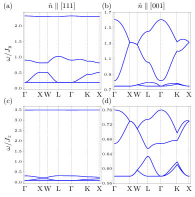
Figure 2: Linear spin wave spectra under external magnetic fields along $[111]$ (a,c) and $[001]$ (b,d) direction. The corresponding classical ground states are “1-in 3-out” and “2-in 2-out”, respectively. (a-b) In the octupolar U(1) QSL regime, we set $J_{y}$ as the energy unit and fix ${J^{y}_{\pm}=-0.075J_{y}}$ and ${J^{y}_{\pm\pm}=0.025J_{y}}$. (c-d) In the dipolar U(1) QSL regime, the energy unit is set to be ${J_{z}=1.0}$ with ${J^{z}_{\pm}=-0.075J_{z}}$ and $J^{y}_{\pm\pm}=-0.025J_{z}$. The strength of external field is fixed to ${h=4.0J_{y}}$ (${h=4.0J_{z}}$) in the octupolar (dipolar) regime to ensure the correct spin configuration. We set $\theta=0$.

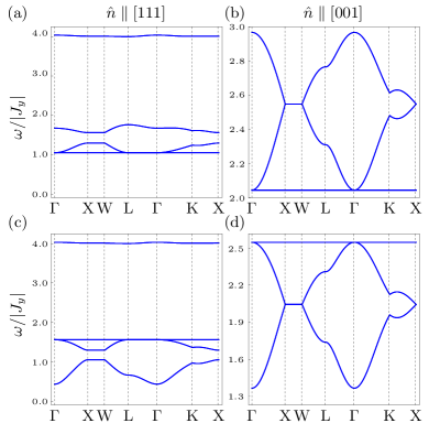
Figure 3: Linear spin wave spectra under external magnetic fields along $[111]$ (a,c) and $[001]$ (b,d) directions. we take ${J_{x}=J_{z}=J_{xz}=0}$ and the magnetic field strength $h=8.0|J_{y}|$ to ensure the “1-in 3-out” and “2-in 2-out” classical spin ground states, respectively. In (a-b) we set ${J_{y}=1}$ as the energy unit and in (c-d) we set ${J_{y}=-1}$.

In our illustrative calculations, we keep ${\theta=0}$ as the previous sections for simplicity. Without losing generality, we set ${J_{y}=1.0}$ and ${J_{z}=1.0}$ as the energy unit for the octupolar and dipolar U(1) QSLs, respectively. Other parameters are set to be ${J^{y}_{\pm}=-0.075J_{y}}$, ${J^{y}_{\pm\pm}=0.025J_{y}}$ and ${J^{z}_{\pm}=-0.05J_{z}}$, ${J^{z}_{\pm\pm}=-0.025J_{z}}$ in order to guarantee the predominance of $\tilde{J}_{y}$ or $\tilde{J}_{z}$ in each case. In both cases, the strength of the magnetic field is fixed to ${h=4.0J_{y}}$ (or ${h=4.0J_{z}}$) which is strong enough to ensure the magnetic ground state is a “1-in 3-out” spin configuration. Diagonalizing the quadratic Hamiltonian $H_{sw}$, one can obtain the linear spin wave spectrum as depicted in Fig. 2(a) and (c). In both the octupolar (a) and dipolar (c) regime, the degenerate bands with the highest energies originate from the deviation of the spin whose local $z$ component is paralleled to the field direction. In the dipolar U(1) QSL, this band is nearly flat and there is a huge gap between other bands while the energy gap is moderate in the octupolar one.

With the same parameters but an external magnetic field along $[001]$ direction, a “2-in 2-out” spin configuration is favored. In this ground state, the spin operators of the 0-th and 3-rd sublattice can be expressed as,

$$S_{i}^{+} = b_{i},\quad S_{i}^{-}=b_{i}^{\dagger},$$ (21)

$$S_{i}^{z} = {1}/{2}-b_{i}^{\dagger}b_{i},$$ (22)

and for the remaining two sublattices, we have

$$S_{i}^{+} = b_{i}^{\dagger},\quad S_{i}^{-}=b_{i},$$ (23)

$$S_{i}^{z} = -{1}/{2}+b_{i}^{\dagger}b_{i}.$$ (24)

As shown in Fig. 2, the bandwidth of linear spin wave spectrum (Fig. 2(b) and (d)) is significantly smaller than the previous case. This is because none of the four local $\hat{z}$ directions in one magnetic unit cell is parallel to the external field. There is a reduced energy cost of spin flipping. In the dipolar regime as shown in Fig. 2(d), the bandwidth is much smaller by comparison.

In order to further study the difference between the dipolar and octupolar U(1) QSLs from the perspective of the spin wave excitations, we take the special case with ${J_{x}=J_{z}=J_{xz}=0}$ and calculate the spin wave spectrum of a $J_{y}$ related Hamiltonian

$$H=\sum_{\langle ij\rangle}J_{y}S_{i}^{y}S_{j}^{y}-h\sum_{i}(\hat{n}\cdot\hat{z}_{i})S_{i}^{z}.$$ (25)

Here, we set the energy unit to be ${|J_{y}|=1}$ but the sign of $J_{y}$ can be changed. To ensure the same classical spin ground states as we have discussed above, the strength of external magnetic field is fixed to be ${h=8|J_{y}|}$. We show the spin wave results in Fig. 3 where ${J_{y}=1}$ for (a-b) and ${J_{y}=-1}$ for (c-d). Our results could potentially provide a guidance for the future inelastic neutron scattering measurements in the strong magnetic fields.

VI Discussion

The Ce-based pyrochlore QSL materials (Ce₂Sn₂O₇ and Ce₂Zr₂O₇) represent a family of QSL materials whose models are provided theoretically Huang et al. (2014); Li and Chen (2017). The major task would be to establish connections between the theoretical results/understanding and experiments. The main result in this paper is based on the U(1) QSLs with dipole-octupole doublets, and the experimental predictions are the spectroscopic properties. It has been shown that the spinon spectrum could have an enhanced spectral periodicity with a folded Brillouin zone and the proximate orders could break the lattice translational symmetry by doubling the unit cell. Another set of experiments would be thermal Hall transports. As we will explain in a separate paper Zhang et al. (2020) that focuses on thermal Hall effect, we predict that there should be a non-trivial topological thermal Hall effect for “magnetic monopoles” due to the dual Berry phase effect in the dipolar U(1) QSL (or any other spin-ice based U(1) QSL materials) while there is no such topological thermal Hall effect for the “magnetic monopoles” excitations in the octupolar U(1) QSL. The possibility of $\mathbb{Z}_{2}$ QSL is not considered here. Although the region of possible $\mathbb{Z}_{2}$ QSL is tiny on the unfrustrated (sign-problem-free) side Huang et al. (2018), the presence of $\mathbb{Z}_{2}$ QSL on the frustrated side is not so clear. Thus, $\mathbb{Z}_{2}$ QSL may still be possible, and the spectrum would be fully gapped. This may be examined carefully with the detailed specific heat measurements.

For the XYZ model on the pyrochlore lattice, it is ready to see that the model reduces to the Heisenberg model when all three couplings are equal. The ground state of the pyrochlore lattice Heisenberg model is one of the hardest problems in quantum magnetism. From the property of the XYZ model, one could at least conclude that the ground state for the Heisenberg model cannot be the $\pi$-flux U(1) QSL for the XXZ model in the frustrated regime. This is because the three spin components have different physical meanings in the emergent spinon-gauge description while the three spin components are symmetrically related by the SU(2) spin rotation at the Heisenberg point.

Appendix A Coordinate system

The centers of the corner-sharing tetrahedra in the pyrochlore lattice constitute a diamond structure with two sublattices, which we denote I and II; see Fig. 4. We choose the origins of the two sublattices as follows,

$${\textbf{O}}_{\rm I} = \left(0,0,0\right),$$ (26)

$${\textbf{O}}_{\rm II} = \left(\frac{1}{4},\frac{1}{4},\frac{1}{4}\right).$$ (27)

The basis vectors of the diamond lattices are taken to be

$${\textbf{a}}_{1} = \left(0,\frac{1}{2},\frac{1}{2}\right),$$ (28)

$${\textbf{a}}_{2} = \left(\frac{1}{2},0,\frac{1}{2}\right),$$ (29)

$${\textbf{a}}_{3} = \left(\frac{1}{2},\frac{1}{2},0\right).$$ (30)

$\mu$	0	1	2	3
$\hat{x}_{\mu}$	$\frac{1}{\sqrt{2}}[\bar{1}10]$	$\frac{1}{\sqrt{2}}[\bar{1}\bar{1}0]$	$\frac{1}{\sqrt{2}}[110]$	$\frac{1}{\sqrt{2}}[1\bar{1}0]$
$\hat{y}_{\mu}$	$\frac{1}{\sqrt{6}}[\bar{1}\bar{1}2]$	$\frac{1}{\sqrt{6}}[\bar{1}1\bar{2}]$	$\frac{1}{\sqrt{6}}[1\bar{1}\bar{2}]$	$\frac{1}{\sqrt{6}}[112]$
$\hat{z}_{\mu}$	$\frac{1}{\sqrt{3}}[111]$	$\frac{1}{\sqrt{3}}[1\bar{1}\bar{1}]$	$\frac{1}{\sqrt{3}}[\bar{1}1\bar{1}]$	$\frac{1}{\sqrt{3}}[\bar{1}\bar{1}1]$

Table 1: Local coordinate frames for the four sublattices on the pyrochlore lattice. The local $\hat{x}$ and $\hat{y}$ directions are not really used in this work because the transverse spin components of local moments are octupolar moments and are defined in the internal spin space.

For each site of the I (II) sublattice there are four vertices of the II (I) sublattice that are nearest neighbors to it, with displacement vectors

$$\eta_{{\textbf{r}}}\,{\textbf{e}}_{0} = \frac{\eta_{{\textbf{r}}}}{4}\left(+1,+1,+1\right),$$ (31)

$$\eta_{{\textbf{r}}}\,{\textbf{e}}_{1} = \frac{\eta_{{\textbf{r}}}}{4}\left(+1,-1,-1\right),$$ (32)

$$\eta_{{\textbf{r}}}\,{\textbf{e}}_{2} = \frac{\eta_{{\textbf{r}}}}{4}\left(-1,+1,-1\right),$$ (33)

$$\eta_{{\textbf{r}}}\,{\textbf{e}}_{3} = \frac{\eta_{{\textbf{r}}}}{4}\left(-1,-1,+1\right),$$ (34)

where $\eta_{{\textbf{r}}}=\pm 1$ for r in sublattice I and II, respectively. At the midpoint of each of such bonds, there is a vertex of the pyrochlore lattice. Correspondingly, we define the local coordinate systems on the four sublattices of the pyrochlore lattice, as summarized in the Table 1.

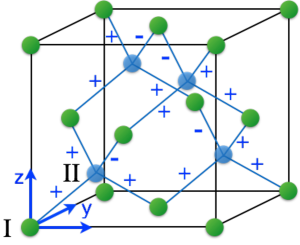
Figure 4: (Color online.) The diamond lattice formed by the tetrahedral centers of the pyrochlore lattice. The choice of spinon hopping is labelled in the plot.

Appendix B Gauge pattern for octupolar U(1)_π QSL state and Bloch hamiltonian

As pointed out in the literature Lee et al. (2012); Chen (2017), in the frustrated regime $J_{\pm}<0$ of the XYZ model (see Eqs. (3, 4)) the ground state has $\pi$-flux within an elementary hexagon. Within the gauge mean field theory, recall that the $s^{\pm}$ operators are gauge string operators, $s^{\pm}_{{\textbf{r}},{\textbf{r}}^{\prime}}=\frac{1}{2}e^{\pm iA_{{\textbf{r}},{\textbf{r}}^{\prime}}}$. We take the following gauge choice for the $\pi$-flux state,

$$A_{{\textbf{r}},{\textbf{r}}+{\textbf{e}}_{\mu}}=\epsilon_{\mu}{\textbf{Q}}\cdot{\textbf{r}},$$ (35)

where $\epsilon=(0110)$, ${\textbf{Q}}=2\pi(100)$, and r belongs to the I sublattice, as illustrated in Fig. 4.

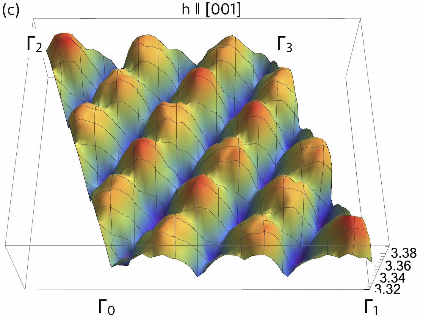
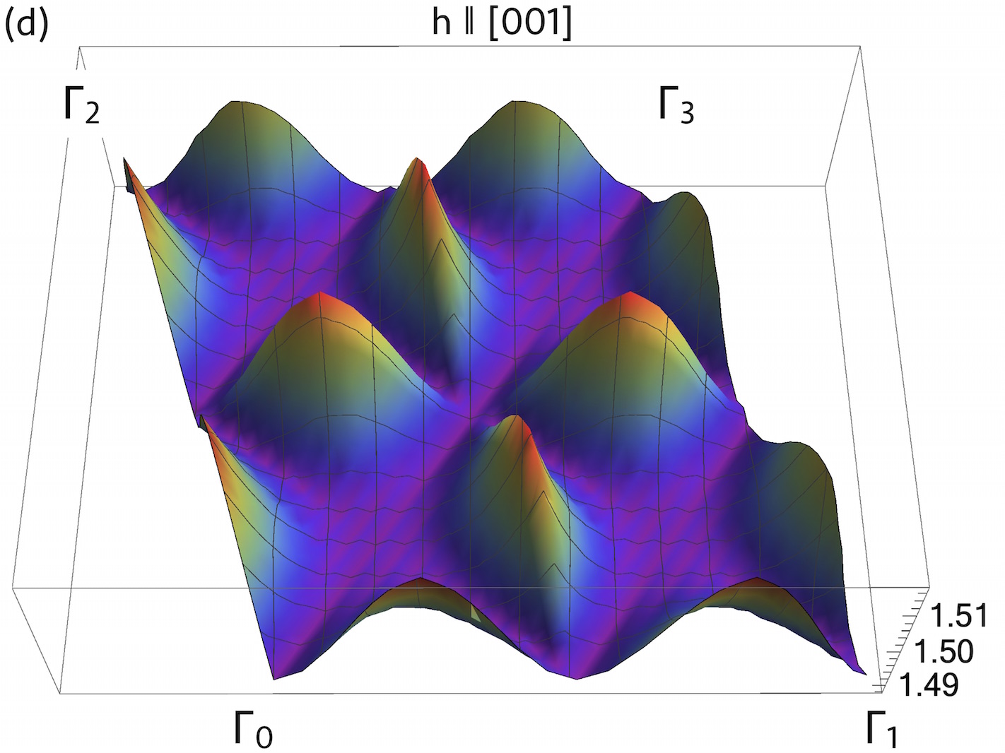
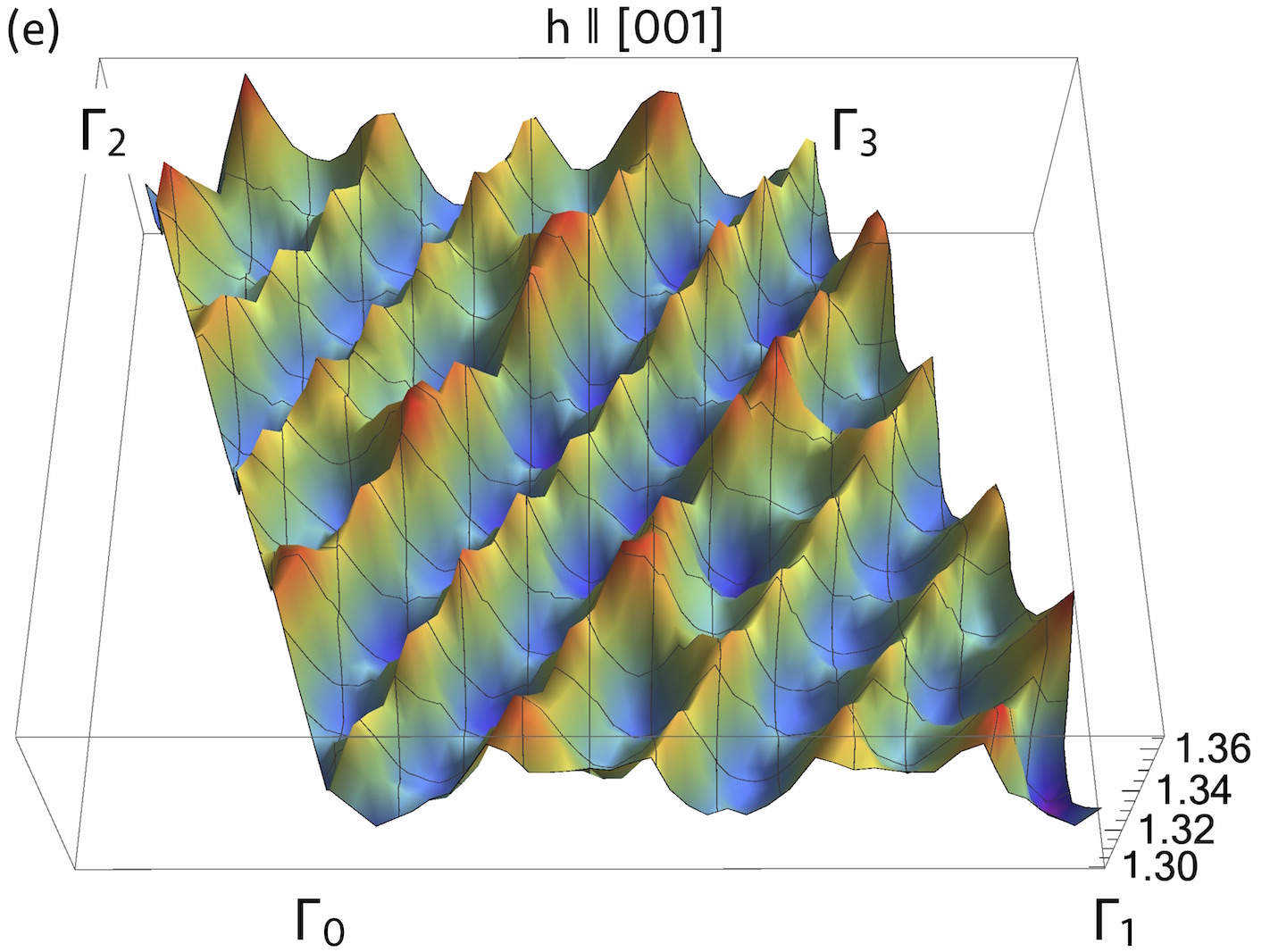
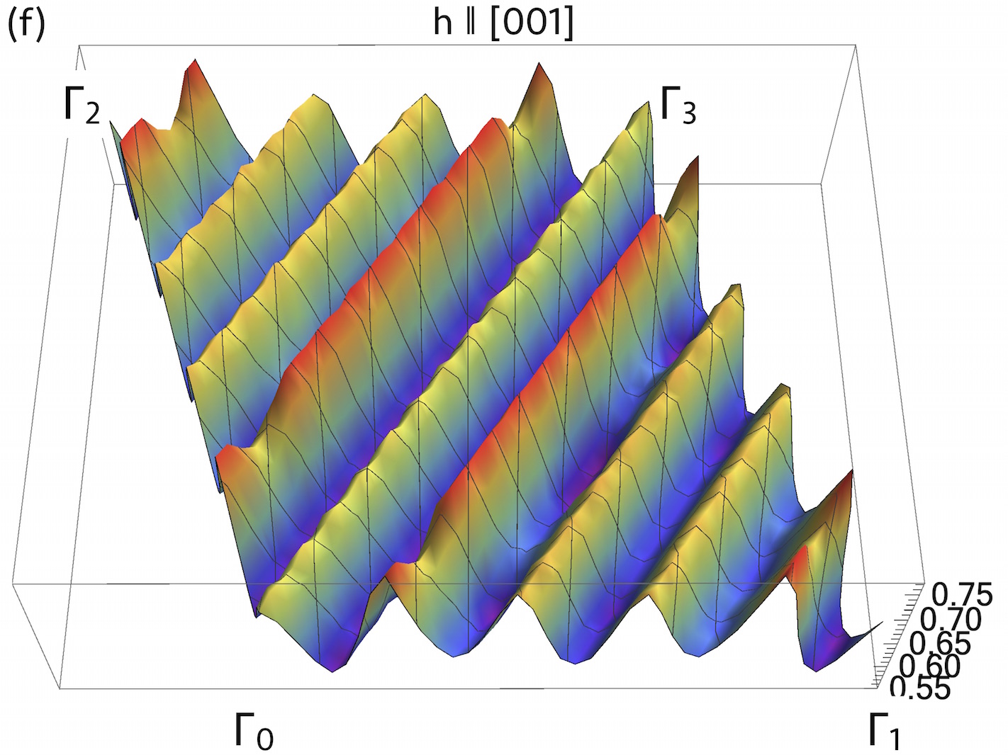
Figure 5: (Color online.) The upper (a, b, c) and lower (d, e, f) excitation edges of the two-spinon continuum in the octupolar U(1)_π QSL, for fields along the [001] direction. We fix $J_{\pm}^{y}=-0.33J_{y},J_{\pm\pm}^{y}=0,\theta=0$, and take $h=0.0J_{y}$ in (a, d), $h=0.2J_{y}$ in (b, e), and $h=1.0J_{y}$ in (c, f).

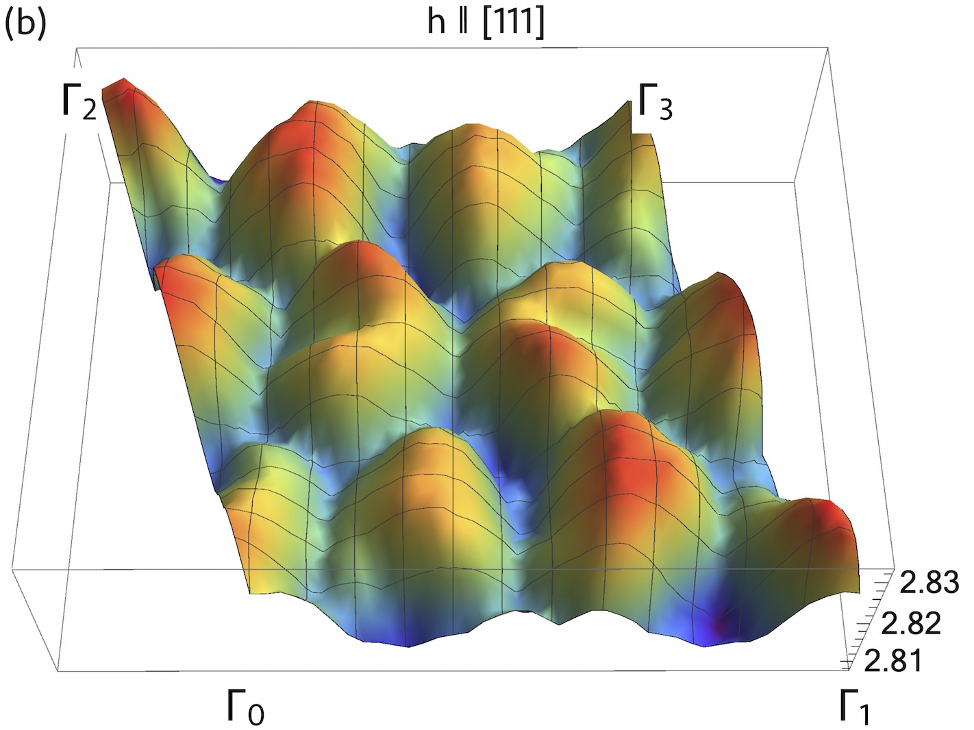
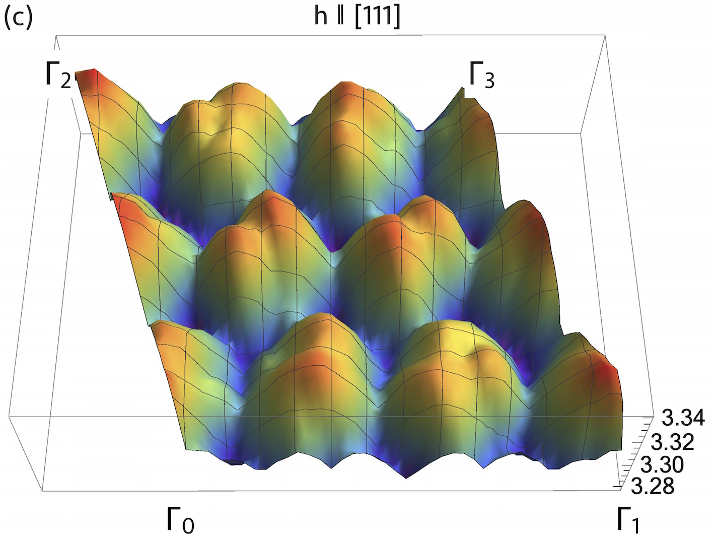
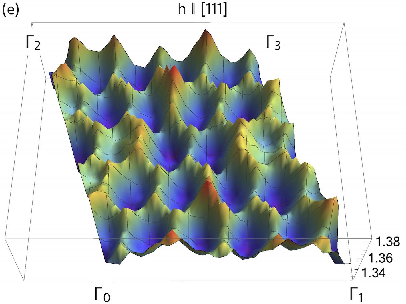
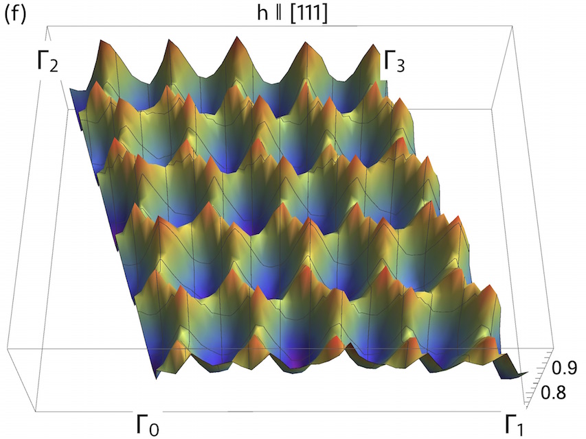
Figure 6: (Color online.) The upper (a, b, c) and lower (d, e, f) excitation edges of the two-spinon continuum in the octupolar U(1)_π QSL, for fields along the [111] direction. We fix $J_{\pm}^{y}=-0.33J_{y},J_{\pm\pm}^{y}=0,\theta=0$, and take $h=0.0J_{y}$ in (a, d), $h=0.2J_{y}$ in (b, e), and $h=1.0J_{y}$ in (c, f).

Because of the $\pi$-flux and the choice of Q, the unit cell doubles in the $x$-direction. Correspondingly, there are four sublattices of the system, which we term ${\rm I},\pm$ and ${\rm II},\pm$. Specifically, a site on the origional I sublattice at r belongs to the ${\rm I},+$ (${\rm I},-$) sublattice if ${\textbf{Q}}\cdot({\textbf{r}}-{\textbf{O}}_{\rm I})$ is an even (odd) multiple of $\pi$; and this is similarly for a site in the II sublattice.

We focus on $H_{y}$ within the frustrated regime $J_{\pm}<0$ and $\theta=0$. Under this fixed gauge, the spinon action is Lee et al. (2012)

$$\mathcal{S} = \int d\tau\left[\sum_{{\textbf{r}}}\frac{1}{2\tilde{J}_{y}}\partial_{\tau}\Phi^{\ast}_{{\textbf{r}}}\partial_{\tau}\Phi_{{\textbf{r}}}+\lambda\sum_{{\textbf{r}}}\left(|\Phi_{{\textbf{r}}}|^{2}-1\right)-J_{\pm}\sum_{\textbf{r}}\sum_{\mu\neq\nu}\left(\Phi^{\dagger}_{{\textbf{r}}+\eta_{\textbf{r}}{\textbf{e}}_{\mu}}\Phi^{\phantom{\dagger}}_{{\textbf{r}}+\eta_{\textbf{r}}{\textbf{e}}_{\nu}}s^{-\eta_{\textbf{r}}}_{{\textbf{r}},{\textbf{r}}+\eta_{\textbf{r}}{\textbf{e}}_{\mu}}s^{+\eta_{\textbf{r}}}_{{\textbf{r}},{\textbf{r}}+\eta_{\textbf{r}}{\textbf{e}}_{\nu}}\right)\right]$$ (36)

$$= \sum_{{\textbf{k}}}\int\frac{d\omega}{2\pi}\,\bm{\Phi}^{\dagger}_{{\textbf{k}}}G_{{\textbf{k}},\omega}\bm{\Phi}^{\phantom{\dagger}}_{{\textbf{k}}}$$

where

$$G_{{\textbf{k}},\omega}=\left[\left(\frac{\omega^{2}}{2\tilde{J}_{y}}+\lambda\right){\textbf{I}}_{4\times 4}+\begin{pmatrix}H_{\rm I,I}({\textbf{k}})&H_{\rm I,II}({\textbf{k}})\\ H_{\rm II,I}({\textbf{k}})&H_{\rm II,II}({\textbf{k}})\end{pmatrix}\right],\quad\bm{\Phi}_{{\textbf{k}}}=\begin{pmatrix}\Phi^{\phantom{\dagger}}_{{\rm I},+}({\textbf{k}})\\ \Phi^{\phantom{\dagger}}_{{\rm I},-}({\textbf{k}})\\ \Phi^{\phantom{\dagger}}_{{\rm II},+}({\textbf{k}})\\ \Phi^{\phantom{\dagger}}_{{\rm II},-}({\textbf{k}})\\ \end{pmatrix},$$ (37)

and

$$H_{\rm I,I}({\textbf{k}}) = -J_{\pm}\begin{pmatrix}+\cos\frac{k_{y}}{2}\cos\frac{k_{z}}{2}&-\sin\frac{k_{x}}{2}\sin\frac{k_{y}}{2}-i\cos\frac{k_{x}}{2}\cos\frac{k_{z}}{2}\\ -\sin\frac{k_{x}}{2}\sin\frac{k_{y}}{2}+i\cos\frac{k_{x}}{2}\cos\frac{k_{z}}{2}&-\cos\frac{k_{y}}{2}\cos\frac{k_{z}}{2}\end{pmatrix},$$ (38)

$$H_{\rm II,II}({\textbf{k}}) = -J_{\pm}\begin{pmatrix}-\sin\frac{k_{y}}{2}\sin\frac{k_{z}}{2}&+\cos\frac{k_{x}}{2}\cos\frac{k_{y}}{2}-i\cos\frac{k_{z}}{2}\sin\frac{k_{x}}{2}\\ +\cos\frac{k_{x}}{2}\cos\frac{k_{y}}{2}+i\cos\frac{k_{z}}{2}\sin\frac{k_{x}}{2}&+\sin\frac{k_{y}}{2}\sin\frac{k_{z}}{2}\end{pmatrix},$$ (39)

$$H_{\rm I,II}({\textbf{k}}) = \frac{h}{4}\begin{pmatrix}+e^{+i{\textbf{k}}\cdot{\textbf{e}}_{0}}({\textbf{n}}\cdot{\textbf{e}}_{0})+e^{+i{\textbf{k}}\cdot{\textbf{e}}_{1}}({\textbf{n}}\cdot{\textbf{e}}_{1})&+e^{+i{\textbf{k}}\cdot{\textbf{e}}_{2}}({\textbf{n}}\cdot{\textbf{e}}_{2})+e^{+i{\textbf{k}}\cdot{\textbf{e}}_{3}}({\textbf{n}}\cdot{\textbf{e}}_{3})\\ -e^{+i{\textbf{k}}\cdot{\textbf{e}}_{2}}({\textbf{n}}\cdot{\textbf{e}}_{2})+e^{+i{\textbf{k}}\cdot{\textbf{e}}_{3}}({\textbf{n}}\cdot{\textbf{e}}_{3})&+e^{+i{\textbf{k}}\cdot{\textbf{e}}_{0}}({\textbf{n}}\cdot{\textbf{e}}_{0})-e^{+i{\textbf{k}}\cdot{\textbf{e}}_{1}}({\textbf{n}}\cdot{\textbf{e}}_{1})\end{pmatrix},$$ (40)

$$H_{\rm II,I}({\textbf{k}}) = \frac{h}{4}\begin{pmatrix}+e^{-i{\textbf{k}}\cdot{\textbf{e}}_{0}}({\textbf{n}}\cdot{\textbf{e}}_{0})+e^{-i{\textbf{k}}\cdot{\textbf{e}}_{1}}({\textbf{n}}\cdot{\textbf{e}}_{1})&-e^{-i{\textbf{k}}\cdot{\textbf{e}}_{2}}({\textbf{n}}\cdot{\textbf{e}}_{2})+e^{-i{\textbf{k}}\cdot{\textbf{e}}_{3}}({\textbf{n}}\cdot{\textbf{e}}_{3})\\ +e^{-i{\textbf{k}}\cdot{\textbf{e}}_{2}}({\textbf{n}}\cdot{\textbf{e}}_{2})+e^{-i{\textbf{k}}\cdot{\textbf{e}}_{3}}({\textbf{n}}\cdot{\textbf{e}}_{3})&+e^{-i{\textbf{k}}\cdot{\textbf{e}}_{0}}({\textbf{n}}\cdot{\textbf{e}}_{0})-e^{-i{\textbf{k}}\cdot{\textbf{e}}_{1}}({\textbf{n}}\cdot{\textbf{e}}_{1})\end{pmatrix}.$$ (41)

Here $\lambda$ is a Lagrange multiplier to ensure the (relaxed) spinon occupation number constraint, $\sum_{{\textbf{r}}}(|\Phi_{{\textbf{r}}}|^{2}-1)=0$. Now all $\Phi$-$\Phi$ correlation functions (including the dynamic spin structure factor) can be computed from this action.

Appendix C Fields along other directions and comparison with octupolar U(1)₀ QSL

Here we include the results of the upper and lower excitations for external fields along $[001]$ (Fig. 5) and $[111]$ (Fig. 6) directions. Enhanced periodicity is also observed in these cases, regardless of the field direction.

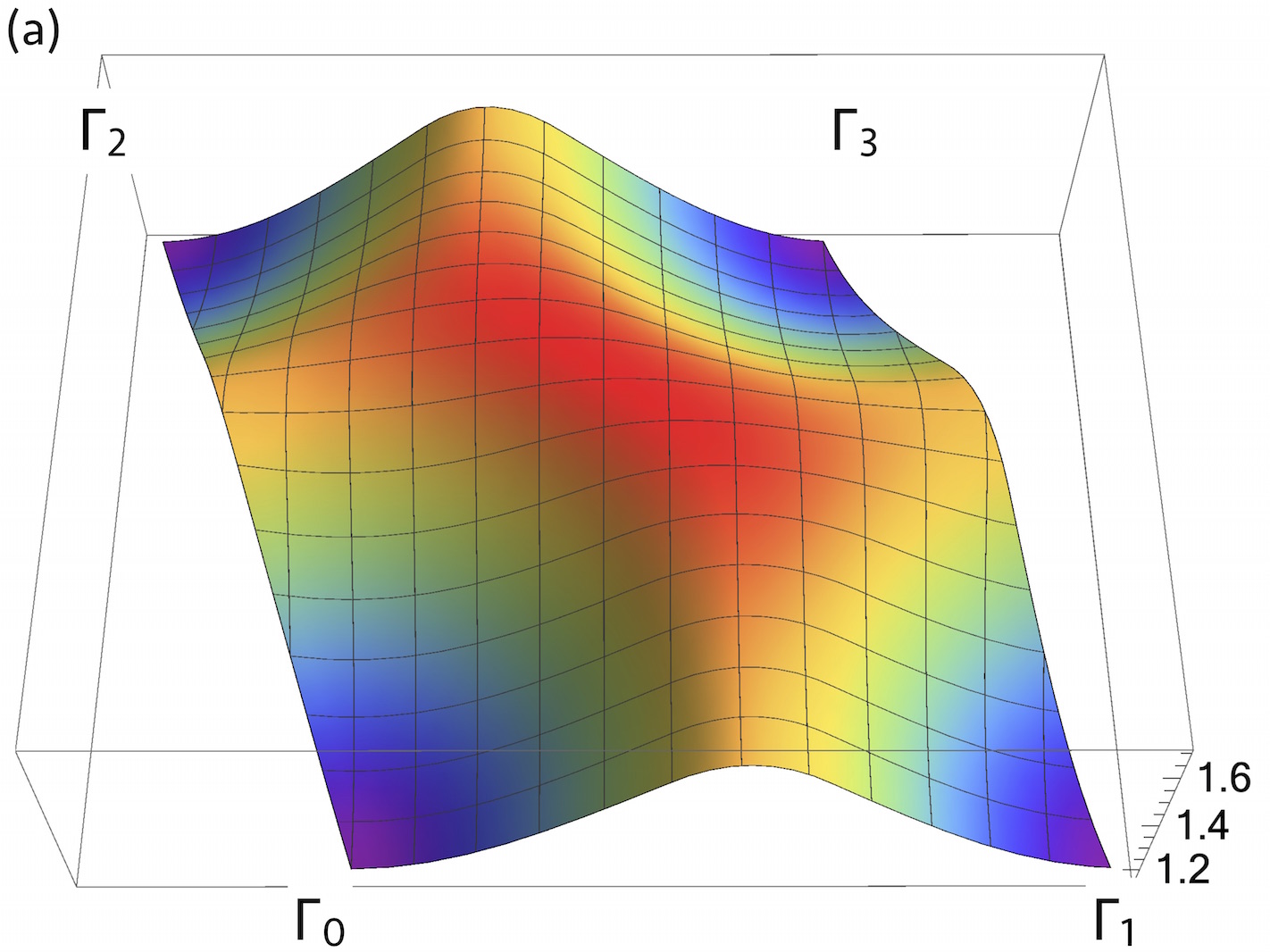
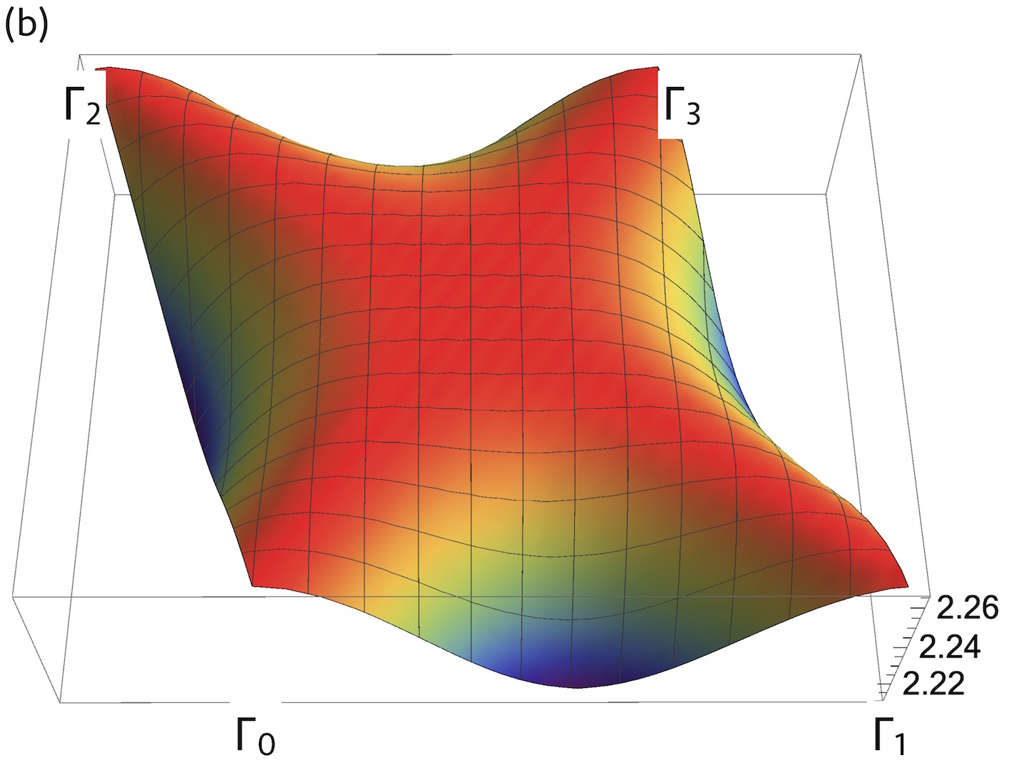
Figure 7: (Color online.) The upper (a) and lower (b) excitation edges of the two-spinon continuum in the octupolar $0$-flux U(1) QSL state. We fix $J_{\pm}^{y}=0.12J_{y},J_{\pm\pm}^{y}=0$ and $h=0.0J_{y}$. The energy unit is set to be $J_{y}$.

As a comparison, we also present the excitation edge for the octupolar $0$-flux U(1) QSL state, where the enhanced spectral periodicity is not observed; see Fig. 7.

References

- Wen (2007) Xiao-Gang Wen, Quantum Field Theory of Many-body Systems: From the Origin of Sound to an Origin of Light and Electrons (Oxford Graduate Texts), reissue ed. (Oxford University Press, USA, 2007).
- Wen (2002) Xiao-Gang Wen, “Quantum orders and symmetric spin liquids,” Phys. Rev. B 65, 165113 (2002).
- Essin and Hermele (2013) Andrew M. Essin and Michael Hermele, “Classifying fractionalization: Symmetry classification of gapped spin liquids in two dimensions,” Phys. Rev. B 87, 104406 (2013).
- Mesaros and Ran (2013) Andrej Mesaros and Ying Ran, “Classification of symmetry enriched topological phases with exactly solvable models,” Phys. Rev. B 87, 155115 (2013).
- Levin and Wen (2005) Michael A. Levin and Xiao-Gang Wen, “String-net condensation: A physical mechanism for topological phases,” Phys. Rev. B 71, 045110 (2005).
- Qi et al. (2019) Yang Qi, Chao-Ming Jian, and Chenjie Wang, “Folding approach to topological order enriched by mirror symmetry,” Phys. Rev. B 99, 085128 (2019).
- Chen and Hermele (2016) Xie Chen and Michael Hermele, “Symmetry fractionalization and anomaly detection in three-dimensional topological phases,” Phys. Rev. B 94, 195120 (2016).
- Chen (2017a) Xie Chen, “Symmetry fractionalization in two dimensional topological phases,” Reviews in Physics 2, 3 – 18 (2017a).
- Molavian et al. (2007) Hamid R. Molavian, Michel J. P. Gingras, and Benjamin Canals, “Dynamically Induced Frustration as a Route to a Quantum Spin Ice State in via Virtual Crystal Field Excitations and Quantum Many-Body Effects,” Phys. Rev. Lett. 98, 157204 (2007).
- Ross et al. (2011) Kate Ross, Lucile Savary, Bruce Gaulin, and Leon Balents, “Quantum Excitations in Quantum Spin Ice,” Phys. Rev. X 1, 021002 (2011).
- Benton et al. (2012) Owen Benton, Olga Sikora, and Nic Shannon, “Seeing the light: Experimental signatures of emergent electromagnetism in a quantum spin ice,” Phys. Rev. B 86, 075154 (2012).
- Fritsch et al. (2014) K. Fritsch, E. Kermarrec, K. A. Ross, Y. Qiu, J. R. D. Copley, D. Pomaranski, J. B. Kycia, H. A. Dabkowska, and B. D. Gaulin, “Temperature and magnetic field dependence of spin-ice correlations in the pyrochlore magnet ,” Phys. Rev. B 90, 014429 (2014).
- Arpino et al. (2017) K. E. Arpino, B. A. Trump, A. O. Scheie, T. M. McQueen, and S. M. Koohpayeh, “Impact of stoichiometry of on its physical properties,” Phys. Rev. B 95, 094407 (2017).
- MacLaughlin et al. (2015) D. E. MacLaughlin, O. O. Bernal, Lei Shu, Jun Ishikawa, Yosuke Matsumoto, J.-J. Wen, M. Mourigal, C. Stock, G. Ehlers, C. L. Broholm, Yo Machida, Kenta Kimura, Satoru Nakatsuji, Yasuyuki Shimura, and Toshiro Sakakibara, “Unstable spin-ice order in the stuffed metallic pyrochlore ,” Phys. Rev. B 92, 054432 (2015).
- Wen et al. (2017) J.-J. Wen, S. M. Koohpayeh, K. A. Ross, B. A. Trump, T. M. McQueen, K. Kimura, S. Nakatsuji, Y. Qiu, D. M. Pajerowski, J. R. D. Copley, and C. L. Broholm, “Disordered Route to the Coulomb Quantum Spin Liquid: Random Transverse Fields on Spin Ice in ,” Phys. Rev. Lett. 118, 107206 (2017).
- Applegate et al. (2012) R. Applegate, N. R. Hayre, R. R. P. Singh, T. Lin, A. G. R. Day, and M. J. P. Gingras, “Vindication of as a Model Exchange Quantum Spin Ice,” Phys. Rev. Lett. 109, 097205 (2012).
- Benton (2018) Owen Benton, “Instabilities of a u(1) quantum spin liquid in disordered non-kramers pyrochlores,” Phys. Rev. Lett. 121, 037203 (2018).
- Benton (2016) Owen Benton, “Quantum origins of moment fragmentation in ,” Phys. Rev. B 94, 104430 (2016).
- Dunsiger et al. (2011) S. R. Dunsiger, A. A. Aczel, C. Arguello, H. Dabkowska, A. Dabkowski, M.-H. Du, T. Goko, B. Javanparast, T. Lin, F. L. Ning, H. M. L. Noad, D. J. Singh, T. J. Williams, Y. J. Uemura, M. J. P. Gingras, and G. M. Luke, “Spin ice: Magnetic excitations without monopole signatures using muon spin rotation,” Phys. Rev. Lett. 107, 207207 (2011).
- Lhotel et al. (2014) E. Lhotel, S. R. Giblin, M. R. Lees, G. Balakrishnan, L. J. Chang, and Y. Yasui, “First-order magnetic transition in ,” Phys. Rev. B 89, 224419 (2014).
- Chang et al. (2014) Lieh-Jeng Chang, Martin R. Lees, Isao Watanabe, Adrian D. Hillier, Yukio Yasui, and Shigeki Onoda, “Static magnetic moments revealed by muon spin relaxation and thermodynamic measurements in the quantum spin ice ,” Phys. Rev. B 89, 184416 (2014).
- Yasui et al. (2003) Yukio Yasui, Minoru Soda, Satoshi Iikubo, Masafumi Ito, Masatoshi Sato, Nobuko Hamaguchi, Taku Matsushita, Nobuo Wada, Tetsuya Takeuchi, Naofumi Aso, and Kazuhisa Kakurai, “Ferromagnetic Transition of Pyrochlore Compound Yb2Ti2O7,” Journal of the Physical Society of Japan 72, 3014–3015 (2003).
- Sibille et al. (2018) Romain Sibille, Nicolas Gauthier, Han Yan, Monica Ciomaga Hatnean, Jacques Ollivier, Barry Winn, Uwe Filges, Geetha Balakrishnan, Michel Kenzelmann, Nic Shannon, and Tom Fennell, “Experimental signatures of emergent quantum electrodynamics in a quantum spin ice,” Nature Physics 14, 711–715 (2018).
- Hao et al. (2014) Zhihao Hao, Alexandre G. R. Day, and Michel J. P. Gingras, “Bosonic many-body theory of quantum spin ice,” Phys. Rev. B 90, 214430 (2014).
- Wan and Tchernyshyov (2012) Yuan Wan and Oleg Tchernyshyov, “Quantum Strings in Quantum Spin Ice,” Phys. Rev. Lett. 108, 247210 (2012).
- Onoda and Tanaka (2010) Shigeki Onoda and Yoichi Tanaka, “Quantum Melting of Spin Ice: Emergent Cooperative Quadrupole and Chirality,” Phys. Rev. Lett. 105, 047201 (2010).
- Lantagne-Hurtubise et al. (2017) Étienne Lantagne-Hurtubise, Subhro Bhattacharjee, and R. Moessner, “Electric field control of emergent electrodynamics in quantum spin ice,” Phys. Rev. B 96, 125145 (2017).
- Khemani et al. (2012) V. Khemani, R. Moessner, S. A. Parameswaran, and S. L. Sondhi, “Bionic coulomb phase on the pyrochlore lattice,” Phys. Rev. B 86, 054411 (2012).
- Udagawa and Moessner (2018) Masafumi Udagawa and Roderich Moessner, “Spectrum of itinerant fractional excitations in quantum spin ice,” arXiv:1811.00199 (2018).
- Curnoe (2008) S. H. Curnoe, “Structural distortion and the spin liquid state in ,” Phys. Rev. B 78, 094418 (2008).
- Onoda and Tanaka (2011) Shigeki Onoda and Yoichi Tanaka, “Quantum fluctuations in the effective pseudospin- model for magnetic pyrochlore oxides,” Phys. Rev. B 83, 094411 (2011).
- Onoda (2011) Shigeki Onoda, “Effective quantum pseudospin-1/2 model for yb pyrochlore oxides,” Journal of Physics: Conference Series 320, 012065 (2011).
- Huang et al. (2014) Yi-Ping Huang, Gang Chen, and Michael Hermele, “Quantum Spin Ices and Topological Phases from Dipolar-Octupolar Doublets on the Pyrochlore Lattice,” Phys. Rev. Lett. 112, 167203 (2014), arXiv:1311.1231 [cond-mat.str-el] .
- Castelnovo1 et al. (2008) C. Castelnovo1, R. Moessner, and S. L. Sondhi, “Magnetic monopoles in spin ice,” Nature 451, 42–45 (2008).
- Castelnovo et al. (2011) C. Castelnovo, R. Moessner, and S. L. Sondhi, “Spin Ice, Fractionalization and Topological Order,” arXiv e-prints , arXiv:1112.3793 (2011), arXiv:1112.3793 [cond-mat.str-el] .
- Bramwell and Gingras (2001) Steven T. Bramwell and Michel J. P. Gingras, “Spin Ice State in Frustrated Magnetic Pyrochlore Materials,” Science 294, 1495–1501 (2001).
- Gingras and McClarty (2014) M. J. P. Gingras and P. A. McClarty, “Quantum spin ice: a search for gapless quantum spin liquids in pyrochlore magnets,” Reports on Progress in Physics 77, 056501 (2014), arXiv:1311.1817 [cond-mat.str-el] .
- Gardner et al. (2010) Jason S. Gardner, Michel J. P. Gingras, and John E. Greedan, “Magnetic pyrochlore oxides,” Rev. Mod. Phys. 82, 53–107 (2010).
- Isakov et al. (2005) S. V. Isakov, R. Moessner, and S. L. Sondhi, “Why spin ice obeys the ice rules,” Phys. Rev. Lett. 95, 217201 (2005).
- Kaiser et al. (2015) V. Kaiser, S. T. Bramwell, P. C. W. Holdsworth, and R. Moessner, “ac wien effect in spin ice, manifest in nonlinear, nonequilibrium susceptibility,” Phys. Rev. Lett. 115, 037201 (2015).
- Hermele et al. (2004) Michael Hermele, Matthew P. Fisher, and Leon Balents, “Pyrochlore photons: The U(1) spin liquid in a S=1/2 three-dimensional frustrated magnet,” Physical Review B 69, 064404 (2004), arXiv:cond-mat/0305401 [cond-mat.str-el] .
- Huse et al. (2003) David A. Huse, Werner Krauth, R. Moessner, and S. L. Sondhi, “Coulomb and Liquid Dimer Models in Three Dimensions,” Phys. Rev. Lett. 91, 167004 (2003), arXiv:cond-mat/0305318 [cond-mat.stat-mech] .
- Motrunich and Senthil (2005) O. I. Motrunich and T. Senthil, “Origin of artificial electrodynamics in three-dimensional bosonic models,” Physical Review B 71, 125102 (2005), arXiv:cond-mat/0407368 [cond-mat.str-el] .
- Savary and Balents (2012) Lucile Savary and Leon Balents, “Coulombic Quantum Liquids in Spin-1/2 Pyrochlores,” Phys. Rev. Lett. 108, 037202 (2012), arXiv:1110.2185 [cond-mat.str-el] .
- Lee et al. (2012) SungBin Lee, Shigeki Onoda, and Leon Balents, “Generic quantum spin ice,” Physical Review B 86, 104412 (2012), arXiv:1204.2262 [cond-mat.str-el] .
- Chen (2017b) Gang Chen, “Spectral periodicity of the spinon continuum in quantum spin ice,” Phys. Rev. B 96, 085136 (2017b).
- Taillefumier et al. (2017) Mathieu Taillefumier, Owen Benton, Han Yan, L. D. C. Jaubert, and Nic Shannon, “Competing Spin Liquids and Hidden Spin-Nematic Order in Spin Ice with Frustrated Transverse Exchange,” Phys. Rev. X 7, 041057 (2017).
- Benton et al. (2018) Owen Benton, L. D. C. Jaubert, Rajiv R. P. Singh, Jaan Oitmaa, and Nic Shannon, “Quantum Spin Ice with Frustrated Transverse Exchange: From a -Flux Phase to a Nematic Quantum Spin Liquid,” Phys. Rev. Lett. 121, 067201 (2018).
- Gao et al. (2019) Bin Gao, Tong Chen, David W. Tam, Chien-Lung Huang, Kalyan Sasmal, Devashibhai T. Adroja, Feng Ye, Huibo Cao, Gabriele Sala, Matthew B. Stone, Christopher Baines, Joel A. T. Barker, Haoyu Hu, Jae-Ho Chung, Xianghan Xu, Sang-Wook Cheong, Manivannan Nallaiyan, Stefano Spagna, M. Brian Maple, Andriy H. Nevidomskyy, Emilia Morosan, Gang Chen, and Pengcheng Dai, “Experimental signatures of a three-dimensional quantum spin liquid in effective spin-1/2 Ce2Zr2O7 pyrochlore,” arXiv e-prints , arXiv:1901.10092 (2019), arXiv:1901.10092 [cond-mat.str-el] .
- Sibille et al. (2015) Romain Sibille, Elsa Lhotel, Vladimir Pomjakushin, Chris Baines, Tom Fennell, and Michel Kenzelmann, “Candidate Quantum Spin Liquid in the Ce3+ Pyrochlore Stannate Ce2 Sn2 O7,” Phys. Rev. Lett. 115, 097202 (2015), arXiv:1502.00662 [cond-mat.str-el] .
- Sibille et al. (2019) Romain Sibille, Nicolas Gauthier, Elsa Lhotel, Victor Porée, Vladimir Pomjakushin, Russell A. Ewings, Toby G. Perring, Jacques Ollivier, Andrew Wildes, Clemens Ritter, Thomas C. Hansen, David A. Keen, Gøran J. Nilsen, Lukas Keller, Sylvain Petit, and Tom Fennell, “A quantum liquid of magnetic octupoles on the pyrochlore lattice,” arXiv e-prints , arXiv:1912.00928 (2019), arXiv:1912.00928 [cond-mat.str-el] .
- Lovesey and van der Laan (2020) S. W. Lovesey and G. van der Laan, “Magnetic multipoles and correlation shortage in pyrochlore cerium stannate,” arXiv e-prints , arXiv:2001.10304 (2020), arXiv:2001.10304 [cond-mat.str-el] .
- Li and Chen (2017) Yao-Dong Li and Gang Chen, “Symmetry enriched U(1) topological orders for dipole-octupole doublets on a pyrochlore lattice,” Physical Review B 95, 041106 (2017).
- Li et al. (2016) Yao-Dong Li, Xiaoqun Wang, and Gang Chen, “Hidden multipolar orders of dipole-octupole doublets on a triangular lattice,” Physical Review B 94, 201114 (2016), arXiv:1608.07008 [cond-mat.str-el] .
- Huang et al. (2018) C.-J. Huang, C. Liu, Z. Meng, Y. Yu, Y. Deng, and G. Chen, “Extended Coulomb liquid of paired hardcore boson model on a pyrochlore lattice,” arXiv e-prints , arXiv:1806.04014 (2018), arXiv:1806.04014 [cond-mat.str-el] .
- Essin and Hermele (2014) Andrew M. Essin and Michael Hermele, “Spectroscopic signatures of crystal momentum fractionalization,” Phys. Rev. B 90, 121102 (2014).
- Chen (2017) Gang Chen, “Dirac’s ”magnetic monopoles” in pyrochlore ice U (1 ) spin liquids: Spectrum and classification,” Physical Review B 96, 195127 (2017), arXiv:1706.04333 [cond-mat.str-el] .
- Chen (2016) Gang Chen, ““Magnetic monopole” condensation of the pyrochlore ice U(1) quantum spin liquid: Application to and ,” Phys. Rev. B 94, 205107 (2016).
- Zhu et al. (2018) Zheng Zhu, Itamar Kimchi, D. N. Sheng, and Liang Fu, “Robust non-Abelian spin liquid and a possible intermediate phase in the antiferromagnetic Kitaev model with magnetic field,” Phys. Rev. B 97, 241110 (2018).
- Zhang et al. (2020) Xiao-Tian Zhang, Yong Hao Gao, Chunxiao Liu, and Gang Chen, “Topological thermal hall effect of magnetic monopoles in the pyrochlore u(1) spin liquid,” Phys. Rev. Research 2, 013066 (2020).