Abstract

Many modern spatial models express the stochastic variation component as a basis expansion with random coefficients. Low rank models, approximate spectral decompositions, multiresolution representations, stochastic partial differential equations and empirical orthogonal functions all fall within this basic framework. Given a particular basis, stochastic dependence relies on flexible modeling of the coefficients. Under a Gaussianity assumption, we propose a graphical model family for the stochastic coefficients by parameterizing the precision matrix. Sparsity in the precision matrix is encouraged using a penalized likelihood framework. Computations follow from a majorization-minimization approach, a byproduct of which is a connection to the graphical lasso. The result is a flexible nonstationary spatial model that is adaptable to very large datasets. We apply the model to two large and heterogeneous spatial datasets in statistical climatology and recover physically sensible graphical structures. Moreover, the model performs competitively against the popular LatticeKrig model in predictive cross-validation, but substantially improves the Akaike information criterion score.

Keywords: spatial basis functions, graphical model, graphical lasso

1 Introduction

Many modern spatial models express the stochastic variation component as a basis expansion with random coefficients. Low rank models, approximate spectral decompositions, multiresolution representations, stochastic partial differential equations and empirical orthogonal functions all fall within this basic framework. The essential difference between these methods is the amount of modeling effort placed on the basis versus the coefficients.

We introduce a novel approach applicable to any model within this framework that allows for nonstationarity and easily adapts to large datasets using off-the-shelf popular basis models. The method allows for straightforward graphical interpretations of the conditional independence structure of the stochastic coefficients.

Most spatial statistical models for an observational process $Y(\mathbf{s})$ with $\mathbf{s}\in\mathbb{R}^{d}$ can be written

$$Y(\mathbf{s})=\mu(\mathbf{s})+Z(\mathbf{s})+\varepsilon(\mathbf{s})$$ (1)

which decomposes the observations into a constant mean function $\mu$, a spatially-correlated random deviation $Z$ and a white noise process $\varepsilon$. Flexible models for the correlated deviation $Z$ are necessary, and much research has been devoted to exploring classes of practical specifications.

In this work we focus on a particularly popular framework where

$$Z(\mathbf{s})=\sum_{j=1}^{\ell}c_{j}\phi_{j}(\mathbf{s})$$ (2)

for $\ell$ fixed basis functions $\phi_{1},\dots,\phi_{\ell}$ and stochastic coefficients $\mathbf{c}=(c_{1},\ldots,c_{\ell})^{\rm T}\sim N(0,Q^{-1})$. Such a spatial basis expansion subsumes many popular approaches including discretized frequency domain models (Fuentes, 2002; Matsuda and Yajima, 2009; Bandyopadhyay and Lahiri, 2009), empirical orthogonal functions (Ch. 5, Cressie and Wikle, 2011), low rank representations (Cressie and Johannesson, 2008; Banerjee et al., 2008b; Guhaniyogi and Banerjee, 2018), multiresolution and wavelet representations (Nychka et al., 2002, 2015; Katzfuss, 2017), and stochastic partial differential equation models (Lindgren et al., 2011; Bolin and Lindgren, 2011).

To set the stage, let us briefly describe some specific models of (2). Fixed rank kriging sets $\ell$ to be relatively small compared to the sample size, uses bisquare functions for $\phi_{i}$, and $Q^{-1}$ is not modeled but rather estimated by minimizing a squared Frobenius distance from an binned empirical covariance matrix (Cressie and Johannesson, 2008). The more recent LatticeKrig model is a multiresolution model that places a large number of compactly supported basis functions with varying supports on a grid and specifies $\mathbf{c}$ as a Gaussian Markov random field (Nychka et al., 2015). Discretized frequency domain approaches and empirical orthogonal functions set the basis functions to be globally supported with independent coefficients (diagonal $Q$), mirroring the spectral representation theorem or the Karhunen-Loeve expansion for stochastic processes. In this work we attempt to relax the modeling assumptions on the structure of the stochastic coefficients $\mathbf{c}$ (equivalently $Q$) by assuming only that they arise from a Gaussian graphical model. We use the well known fact that the graph structure of a multivariate Gaussian is equivalent to the zero/non-zero pattern in the precision matrix $Q$ (Rue and Held, 2005). A major distinction of this work is that we do not specify the structure of the graph, but instead try to infer its edges by estimating the entries of $Q$, while encouraging sparsity using a penalized likelihood estimation framework.

The penalization framework appears straightforward, using an $\ell_{1}$-penalized maximum likelihood estimator for $Q$. However, the corresponding optimization problem is nonconvex, but we show it can be solved efficiently using a majorization-minimization approach where the interior minimization problem corresponds to the graphical lasso problem (Friedman et al., 2008). We perform a relatively detailed simulation study to assess the algorithm and model’s ability to recover unknown graphical structures, and also apply the method to two challenging large and heterogeneous datasets: the first a historical observational dataset of minimum temperatures over a portion of North America, and the second a global reforecast dataset of surface temperature. The results from these real data applications suggest our method can appropriately capture nonstationary spatial correlations with minimal modeling effort.

2 Penalized likelihood estimation

For ease of exposition we suppose $\mu(\mathbf{s})=0$ in (1). Thus the observational model is

$$Y(\mathbf{s})=\sum_{j=1}^{\ell}c_{j}\phi_{j}(\mathbf{s})+\varepsilon(\mathbf{s}).$$ (3)

We suppose we have $m$ independent realizations, $Y(\mathbf{s})=Y_{1}(\mathbf{s}),\ldots,Y_{m}(\mathbf{s})$ of the observational process at spatial locations $\mathbf{s}=\mathbf{s}_{1},\ldots,\mathbf{s}_{n}$. Group a realization as $\mathbf{Y}_{i}=(Y_{i}(\mathbf{s}_{1}),\ldots,Y_{i}(\mathbf{s}_{n}))^{\rm T}$. A matrix representation of the model is

$$\mathbf{Y}_{i}=\Phi\mathbf{c}_{i}+\boldsymbol{\varepsilon}_{i},\quad i=1,\dots,m$$ (4)

where $\Phi$ is an $n\times\ell$ matrix with $(i,j)$th entry $\phi_{j}(\mathbf{s}_{i})$, $\mathbf{c}_{i}=(c_{i1},\ldots,c_{i\ell})^{\rm T}$ are $m$ independent vectors of the stochastic coefficients and $\boldsymbol{\varepsilon}_{i}=(\varepsilon_{i}(\mathbf{s}_{1}),\ldots,\varepsilon_{i}(\mathbf{s}_{n}))^{\rm T}$ are $m$ independent realizations of the white noise process. The stochastic assumptions of our model are that $\varepsilon_{i}$ is a mean zero white noise process with variance $\tau^{2}>0$, commonly referred to as the nugget effect in the geostatistical literature, and that $\mathbf{c}_{i}$ is a mean zero $\ell$-variate multivariate normal random vector with precision matrix $Q$. The zero structure of $Q$ encodes the graphical model for $\mathbf{c}_{i}$.

The model (3) plays a crucial role in modern statistics: it is the framework for a variety of popular statistical techniques including factor analysis, principal component analysis, linear dynamical systems, hidden Markov models, and relevance vector machines (Roweis and Ghahramani, 1999; Tipping, 2001). In the spatial context, there are two main features that arise from using a model of the form (3): first, the resulting model of the spatial field is nonstationary, and second, common computations involving the covariance matrix can be sped up with particular choices for $\Phi$ and $Q$.

2.1 The penalized likelihood

With the $m$ realizations $\mathbf{Y}_{1},\ldots,\mathbf{Y}_{m}$ of (4), twice the negative log-likelihood function can be written, up to multiplicative and additive constants, as

$$\log\det(\Phi Q^{-1}\Phi^{\mathrm{T}}+\tau^{2}I_{n})+\text{tr}(S(\Phi Q^{-1}\Phi^{\mathrm{T}}+\tau^{2}I_{n})^{-1})$$ (5)

where $S=\frac{1}{m}\sum_{i=1}^{m}\mathbf{Y}_{i}\mathbf{Y}_{i}^{\rm T}$ is an empirical covariance matrix.

Our goal is to estimate $Q$ under the assumption that it follows a graphical structure. A few connections are worth noting. When $\Phi=I_{\ell}$ and $\tau^{2}=0$, (5) is, up to the regularization term, the graphical lasso problem studied in (Friedman et al., 2008). In particular, this is equivalent to directly observing $\mathbf{c}_{1},\dots,\mathbf{c}_{m}$. The graphical lasso uses an $\ell_{1}$ penalty to induce a graph structure on $Q$, from which we draw inspiration next. Our situation is substantially more complicated due to observational error and indirect observations of $\mathbf{c}_{i}$ that are modulated by $\Phi$.

Our proposal is to estimate $Q$ by minimizing a penalized version of (5). The estimator of $Q$ is

$$\hat{Q}\in\operatorname*{arg\,min}\limits_{Q\succeq 0}\ \log\det(\Phi Q^{-1}\Phi^{\mathrm{T}}+\tau^{2}I_{n})+\text{tr}(S(\Phi Q^{-1}\Phi^{\mathrm{T}}+\tau^{2}I_{n})^{-1})+\|\Lambda\circ Q\|_{1}.$$ (6)

The notation $Q\succeq 0$ indicates that $Q$ must be positive semidefinite, and $\|\Lambda\circ Q\|_{1}=\sum_{i,j}\Lambda_{ij}|Q_{ij}|$ is a penalty term that enforces sparsity on the elements of $Q$. Here $\Lambda_{ij}$ are nonnegative penalty parameters, with higher values in the matrix $\Lambda$ encouraging more zeros in the estimate. In this paper, we assume that the diagonal elements of $\Lambda$ are zero, reflecting the fact that we are searching for sparsity in the off-diagonal elements of $Q$.

At first glance it is hard to determine whether the problem (6) is convex or nonconvex. We address this issue explicitly in the next section. In either case, it will be difficult to work with the objective function presented in (6) due to the nested inverses surrounding $Q$. Employing a slew of matrix identities allows for the following result, whose proof is kept in the Appendix.

Proposition 1.

The minimizer of (6) is also the minimizer of

$$\log\det\left(Q+\frac{1}{\tau^{2}}\Phi^{\mathrm{T}}\Phi\right)-\log\det Q-\mathrm{tr}\left(\dfrac{1}{\tau^{4}}\Phi^{\mathrm{T}}S\Phi\left(Q+\frac{1}{\tau^{2}}\Phi^{\mathrm{T}}\Phi\right)^{-1}\right)+\|\Lambda\circ Q\|_{1}.$$ (7)

After precomputing the matrix products $\Phi^{\mathrm{T}}\Phi$ and $\Phi^{\mathrm{T}}S\Phi$, evaluating (7) involves inverses and determinants of only $\ell\times\ell$ matrices. This is the essential computational strategy of fixed rank kriging and LatticeKrig which is harnessed in different ways: by making either $\ell$ noticeably smaller than $n$ (fixed rank kriging), or by making $\ell$ extremely large but ensuring the resulting matrices are sparse (LatticeKrig).

2.2 Optimization approach

In the $\ell=1$ case, (7) is a univariate function that is twice differentiable on the positive real line. It is straightforward to select $\Phi^{\mathrm{T}}\Phi$, $\Phi^{\mathrm{T}}S\Phi$, and $\tau^{2}$ so that the second derivative has a negative value at some point along the positive real line. Thus (7) is, in general, a nonconvex function on $Q\succeq 0$. We can, however, show that the four summands in (7) are concave, convex, concave, and convex, respectively, on $Q\succeq 0$; see the Appendix for details. Therefore, the objective function in (7) can be written as

$$\operatorname*{arg\,min}\limits_{Q\succeq 0}f(Q)+g(Q)+\|\Lambda\circ Q\|_{1}$$ (8)

where $f(Q)+\|\Lambda\circ Q\|_{1}$ is convex and $g(Q)$ is concave and differentiable. A natural approach for this nonconvex problem is a Difference-of-Convex (DC) program (Dinh Tao and Le Thi, 1997) where we iteratively linearize the concave part $g(Q)$ at the previous guess $Q_{j}$ and solve the resulting convex problem:

$$Q_{j+1}=\operatorname*{arg\,min}\limits_{Q\succeq 0}\left(f(Q)+\text{tr}(\nabla g(Q_{j})Q)+\|\Lambda\circ Q\|_{1}\right).$$ (9)

Motivating the DC framework requires describing a more general scheme called a majorization-minimization algorithm (Hunter and Lange, 2004). We say that a function $h(\theta)$ is majorized by $m(\theta\mid\theta^{*})$ at $\theta^{*}$ if $h(\theta)\leq m(\theta\mid\theta^{*})$ for all $\theta$ and $h(\theta^{*})=m(\theta^{*}\mid\theta^{*})$. Instead of directly minimizing $h(\theta)$, which can be very complicated, a majorizaton-minimization (MM) algorithm solves a sequence of minimization problems where the majorizing function at the previous guess is minimized:

$$\theta_{j+1}\leftarrow\operatorname*{arg\,min}\limits_{\theta}\ m(\theta\mid\theta_{j}).$$ (10)

Combining (10) with the definition of a majorant yields the inequality

$$h(\theta_{j+1})\leq m(\theta_{j+1}\mid\theta_{j})\leq m(\theta_{j}\mid\theta_{j})=h(\theta_{j})$$

and thus the algorithm is forced to a local minimum (or saddle point) of $h(\theta)$. The most famous instance of the MM algorithm in statistics is the expectation maximization (EM) algorithm, which under this framework uses Jensen’s Inequality to construct majorizing functions for the conditional expectation of log likelihood equations.

Difference-of-convex programming, also called the Concave-Convex-Procedure (CCP), is a subclass of MM where the supporting hyperplane inequality $g(\theta)\leq g(\theta_{j})+\langle\nabla g(\theta_{j}),\theta-\theta_{j}\rangle$ is used to construct a majorizing function when $h(\theta)$ is written as the sum of a convex function and a concave differentiable function $g(\theta)$; i.e., when $h(\theta)$ is a difference of convex functions. An added benefit under the DC framework is that the majorizing function is convex by construction and hence we solve a series of convex optimization problems in each step of (10).

In our likelihood function, the convex part is

$$f(Q)=-\log\det Q$$

and the concave part is

$$g(Q)=\log\det\left(Q+\frac{1}{\tau^{2}}\Phi^{\mathrm{T}}\Phi\right)-\text{tr}\left(\dfrac{1}{\tau^{4}}\Phi^{\mathrm{T}}S\Phi\left(Q+\frac{1}{\tau^{2}}\Phi^{\mathrm{T}}\Phi\right)^{-1}\right),$$

so the DC algorithm (9) becomes

$$Q_{j+1}=\operatorname*{arg\,min}_{Q\succeq 0}\left(-\log\det Q+\text{tr}\left(\nabla g(Q_{j})Q\right)+\|\Lambda\circ Q\|_{1}\right)$$ (11)

where $\nabla g(Q_{j})=\left(I_{\ell}+\left(Q_{j}+\frac{1}{\tau^{2}}\Phi^{\mathrm{T}}\Phi\right)^{-1}\frac{1}{\tau^{4}}\Phi^{\mathrm{T}}S\Phi\right)\left(Q_{j}+\frac{1}{\tau^{2}}\Phi^{\mathrm{T}}\Phi\right)^{-1}$. The inner minimization problem in (11) is well-studied and known in statistics as the graphical lasso problem. The graphical lasso is used to estimate an undirected graphical model (i.e. GMRF neighborhood structure) for a mean zero multivariate Gaussian vector $\mathbf{X}$ under the assumption that we observe $\mathbf{X}$ directly and without noise. The standard graphical lasso estimate is obtained from the penalized negative log likelihood

$$\operatorname*{arg\,min}\limits_{Q\succeq 0}\ -\log\det Q+\text{tr}(S_{\mathbf{X}}Q)+\|\Lambda\circ Q\|_{1}$$ (12)

where $S_{\mathbf{X}}$ is the sample covariance of the realizations of $\mathbf{X}$. In effect, we have shown that the graphical structure of $Q$ given realizations from $\Phi\mathbf{c}+\boldsymbol{\varepsilon}$ can be discerned through a Concave-Convex-Procedure where the inner solve is a graphical lasso problem with the “sample covariance” matrix as a function of the previous guess $Q_{j}$.

A variety of numerical techniques have been proposed for the graphical lasso. (Yuan and Lin, 2007) and (Banerjee et al., 2008a) both use interior point methods, but the latter examine the dual problem of (12)

$$\operatorname*{arg\,min}\limits_{\|U\|_{\infty}\leq\lambda}\ -\log\det(S+U)-n,$$ (13)

where $\|U\|_{\infty}$ is the maximum absolute element of the matrix $U$, and solve (13) one column at a time via quadratic programming. (Friedman et al., 2008) takes an identical approach but writes the dual problem of the columnwise minimization as a lasso regression, which they solve quickly using their own coordinate descent algorithm (Friedman et al., 2007). This implementation is available in the popular R package glasso.

Advances in solving (12) in recent years have stemmed from the use of second-order methods that incorporate Hessian information instead of simply the gradient. A current state of the art algorithm is QUIC (Hsieh et al., 2014) which also features an R package of the same name. Briefly, the QUIC algorithm uses coordinate descent to search for a Newton direction based on a quadratic expansion about the previous guess and then an Armijo rule to select the corresponding stepsize. During the coordinate descent update, only a set of free variables are updated, making the procedure particularly effective when $Q$ is sparse. In the appendix, we provide R Code to solve (11) using QUIC. A very recent paper (Fattahi et al., 2019), accompanied by Matlab code, shows that reformulating (12) as a maximum determinant matrix completion problem is a promising strategy.

2.2.1 Estimating the nugget variance

In practice, we must produce an estimate $\hat{\tau}^{2}$ which is fixed during the algorithm (11). For this purpose we return to the likelihood (5), now rewritten as

$$f(Q,\tau^{2})=\log\det\left(Q+\frac{1}{\tau^{2}}\Phi^{T}\Phi\right)-\log\det Q-\text{tr}\left(\frac{1}{\tau^{4}}\Phi^{T}S\Phi\left(Q+\frac{1}{\tau^{2}}\Phi^{T}\Phi\right)^{-1}\right)+n\log\tau^{2}+\frac{\text{tr}(S)}{\tau^{2}},$$

under the assumption that $Q=\alpha I_{\ell}$ for some parameter $\alpha>0$. The maximizer of $f$ over $\tau^{2}$ and $\alpha$ yields an estimate for the nugget effect of our nonstationary process by an approximation to stationarity through $Q=\alpha I_{\ell}$. Our estimates $\hat{\tau}^{2}$ and $\hat{\alpha}$ were retrieved from an L-BFGS optimization routine via the optim function in R. In the simulation study below this approach is seen to empirically work very well. Jointly estimating a full model of $Q$ and $\tau^{2}$ is complicated and unlikely to result in substantial empirical improvement (see Section 3.1.1).

2.2.2 Estimating the penalty weight

All that remains to specify is the penalty weight matrix $\Lambda$. One option follows Bien and Tibshirani (2011), in which a likelihood-based cross validation approach is used to select $\Lambda$ in the context of estimating a sparse covariance matrix. More formally, suppose we use $k$ folds and consider $t$ penalty matrices $(\Lambda_{1},\dots,\Lambda_{t})$. Let $\hat{Q}_{\Lambda}(S)$ be the estimate we get from applying our algorithm with empirical covariance $S=\frac{1}{m}\sum_{i=1}^{m}\mathbf{Y}_{i}\mathbf{Y}_{i}^{\rm T}$ and penalty $\Lambda$. For $A\subseteq\{1,\dots,m\}$, let $S_{A}=|A|^{-1}\sum_{i\in A}\mathbf{Y}_{i}\mathbf{Y}_{i}^{\rm T}$. We seek $\Lambda$ so that $\alpha(\Lambda)=\ell(\hat{Q}_{\Lambda}(S),S)$ is small, where

$$\ell(Q,S)=\log\det\left(Q+\frac{1}{\tau^{2}}\Phi^{T}\Phi\right)-\log\det Q-\text{tr}\left(\dfrac{1}{\tau^{4}}\Phi^{\mathrm{T}}S\Phi\left(Q+\frac{1}{\tau^{2}}\Phi^{\mathrm{T}}\Phi\right)^{-1}\right)$$ (14)

is the unpenalized likelihood function in (7). The cross validation approach is to partition $\{1,\dots,m\}$ into disjoint sets $\{A_{1},\dots,A_{k}\}$ and select $\hat{\Lambda}=\operatorname*{arg\,min}\limits_{\Lambda\in\{\Lambda_{1},\dots,\Lambda_{t}\}}\hat{\alpha}(\Lambda)$ where $\hat{\alpha}(\Lambda)=k^{-1}\sum_{i=1}^{k}\ell(\hat{Q}_{\Lambda}(S_{A_{i}^{c}}),S_{A_{i}})$.

Another option is through spatial cross validation, where we use training data to estimate estimate $\hat{Q}_{\Lambda_{1}}(S_{\text{train}}),\dots,\hat{Q}_{\Lambda_{t}}(S_{\text{train}})$ and then krige to the held out locations in the testing data. The penalty weight matrix producing the smallest RMSE would then be used in conjunction with the full sample covariance $S$ to obtain the final estimate $\hat{Q}$.

2.2.3 Initial guess and convergence

The nonconvex nature of this problem prohibits use of convergence criterion available for common convex optimization problems. Instead, we say that the DC scheme has “converged” when $\frac{\|Q_{j+1}-Q_{j}\|_{F}}{\|Q_{j}\|_{F}}<\varepsilon$ for some loose tolerance $\varepsilon=0.01$. In this paper, we used the initial guess $Q_{0}=I_{\ell}$, and this choice can produce large diagonal entries $Q_{ii}\gg 0$ since the diagonal penalty weights of $\Lambda$ are set to zero (see results in Section 4.1).

3 Simulation study

This section contains a set of simulation studies to assess the ability of our proposed algorithm to recover unknown precision structures under the model (4). The section is broken into two classes of basis functions – localized bases whose support is spatially compact, and global basis functions that are nonzero over the entire domain. For each class we entertain multiple types of precision structures that are common in the graphical modeling literature.

For each choice of $n$, $\Phi$, and $Q$, the noise-to-signal ratio $\tau^{2}/(\text{tr}(\Phi Q^{-1}\Phi^{\mathrm{T}})/n)$ is fixed at $0.1$ and hence determines the true nugget variance $\tau^{2}$. Our estimated nugget variance $\hat{\tau}^{2}$ is retrieved from Section 2.2.1. Although in these simulations the population mean is zero, in practice it is unknown, so throughout we use the standard unbiased estimator $S$ that includes an empirical demeaning which will reflect practical implications better than using the known mean.

3.1 Local basis

First, we consider a localized problem where we use a basis of compactly supported functions on a grid using the LatticeKrig model setup Nychka et al. (2015), which we briefly describe here: basis functions are compactly supported Wendland functions whose range of support is set so that each function overlaps with 2.5 other basis functions along axial directions. The model basis functions will correspond to either a single level or multiresolution model. In the single level setup, functions are placed on a regular grid. In the multiresolution setup, higher levels of resolution are achieved by increasing the number of basis functions and nodal points (e.g., the second level doubles the number of nodes in each axial direction). The precision matrix $Q$ can be set to approximate Matérn-like behavior, see Nychka et al. (2015) for details.

We specify the variance of the multiresolution levels to behave like an exponential covariance by setting parameter $\nu=0.5$. In LatticeKrig, the precision matrix $Q$ is constructed according to a spatial autoregression parameterized by the value $\alpha$, which we fix at $\alpha=4.05$. For simplicity, we employ no buffer region when constructing the Wendland bases; i.e. there are no basis functions centered outside of the spatial domain. We use the R package LatticeKrig to set up the forementioned basis and precision matrices. A total of $m=500$ realizations from the process (4) under this model are generated, and we repeat this entire spatial data generation process over 30 independent trials.

The spatial domain is $[0,1]\times[0,1]$, and $n$ observation locations are chosen uniformly at random in this domain for different sample sizes $n\in\{100^{2},150^{2},200^{2}\}$. For the single level Wendland basis, we use $\ell\in\{100,225,400\}$ basis functions. Attempting to mirror these dimensions in the multiresolution basis, we use $\ell\in\{119,234,404\}$ which respectively correspond to 1) four multiresolution levels, the coarsest containing 2 Wendland basis functions, 2) three multiresolution levels, the coarsest containing 4 Wendland basis functions and 3) four multiresolution levels, the coarsest containing 3 Wendland basis functions.

We parameterize the penalty matrix $\Lambda$ according to

$$\Lambda_{ij}=\begin{cases}\lambda,&i\neq j,\\ 0,&i=j,\end{cases}$$ (15)

allowing for free estimates of the marginal precision parameters. A 5-fold cross validation as described in Section 2.2.2 is used to select a penalty matrix $\Lambda$ from eight equally spaced values from 0.005 to 0.1. The optimal value is then used with the full sample covariance $S$ in (11) to give a best guess $\hat{Q}$ for the simulated data. To validate our proposed estimation approach we report several summary statistics, each averaged over the 30 trials: the Frobenius norm $\|\hat{Q}-Q\|_{F}/\|Q\|_{F}$, the Kullback-Leibler (KL) divergence $\text{tr}(\hat{Q}Q)-\log\det(\hat{Q}Q)-\ell$, the percentage of zeros in $Q$ that were missed by $\hat{Q}$, the percentage of nonzero elements in $Q$ that were missed by $\hat{Q}$, the estimated nugget effect $\hat{\tau}^{2}$, the true nugget effect $\tau^{2}$, and the estimated and true negative log-likelihoods $f(\hat{Q},\hat{\tau}^{2})$ and $f(Q,\tau^{2})$, where the function $f$ is defined in Section 2.2.1.

Table 1: Simulation study results for the single level case. Scores are averaged over 30 independent trials. Each column represents the number of observation samples, number of basis functions, Frobenius norm, KL divergence, percent of true zeros missed, percent of true nonzeros missed, estimated nugget, true nugget, estimated negative log-likelihood and true negative log-likelihood.

$n$	$\ell$	Frob	KL	$\%$MZ	$\%$MNZ	$\hat{\tau}^{2}$	$\tau^{2}$	$f(\hat{Q},\hat{\tau}^{2})$	$f(Q,\tau^{2})$
	100	0.41	6.5	21.3%	5.3%	0.1	0.1	-12678	-12677
10000	225	0.49	25.9	19.9%	2.0%	0.1	0.1	-12460	-12450
	400	0.72	113.4	4.7%	8.2%	0.1	0.1	-12204	-12220
	100	0.38	5.6	22.3%	5.6%	0.1	0.1	-28889	-28888
22500	225	0.43	20.8	21.1%	2.4%	0.1	0.1	-28601	-28591
	400	0.65	82.4	4.9%	1.0%	0.1	0.1	-28259	-28277
	100	0.37	5.3	22.6%	5.6%	0.1	0.1	-51631	-51630
40000	225	0.41	18.7	21.7%	2.6%	0.1	0.1	-51287	-51277
	400	0.61	69.9	4.9%	1.3%	0.1	0.1	-50876	-50896

Table 2: Simulation study results for the multiple level case. Scores are averaged over 30 independent trials. Each column represents the number of observation samples, number of basis functions, Frobenius norm, KL divergence, percent of true zeros missed, percent of true nonzeros missed, estimated nugget, true nugget, estimated negative log-likelihood and true negative log-likelihood. at the truth.

$n$	$\ell$	Frob	KL	$\%$MZ	$\%$MNZ	$\hat{\tau}^{2}$	$\tau^{2}$	$f(\hat{Q},\hat{\tau}^{2})$	$f(Q,\tau^{2})$
	119	0.82	645	5.6%	6.8%	0.1	0.1	-12866	-12865
10000	234	0.89	2024.6	6.4%	3.7%	0.1	0.1	-12733	-12730
	404	0.85	3789.9	0.07%	2.5%	0.1	0.1	-12719	-12721
	119	0.77	639.7	7.1%	6.4%	0.1	0.1	-29105	-29105
22500	234	0.85	2045.4	10%	3.3%	0.1	0.1	-28935	-28930
	404	0.93	4276.9	0.08%	2.5%	0.1	0.1	-28902	-28907
	119	0.79	634.8	7.8%	6.0%	0.1	0.1	-51866	-51866
40000	234	0.84	1943.2	11.4%	3.0%	0.1	0.1	-51663	-51658
	404	0.94	4438.1	0.09%	2.5%	0.1	0.1	-51612	-51619

3.1.1 Comments

Tables 1 and 2 contain results from this simulation study. We see that estimating the nugget effect $\tau^{2}$ by treating the process as stationary is quite accurate. Estimates under the multiresolution basis are clearly lackluster when compared to the single resolution counterpart. The Frobenius norm and KL divergence tend to increase with the size of $\ell$, but this is to be expected as the dimensions of the target precision matrix $Q$ grow in $\ell$. The percentage of zeros in $Q$ that are missed (i.e. nonzero) in $\hat{Q}$ drops sharply as $\ell$ increases to 400, but this is the consequence of a harsher penalty weight matrix selected in the cross validation scheme.

3.2 Global basis

Next, we consider a spatial basis defined globally, that is, without compact support. In particular, we set up a harmonic basis via the model $\phi_{i}(\mathbf{s})=\cos(2\pi\boldsymbol{\omega}_{i}^{\mathrm{T}}\mathbf{s})$ where the frequencies $\boldsymbol{\omega}_{1},\dots,\boldsymbol{\omega}_{\ell}\in\mathbb{R}^{2}$ are all pairwise combinations of the form $(\frac{k}{\sqrt{n}},\frac{j}{\sqrt{n}})$ for $k,j=1,\dots,\sqrt{\ell}-1$. Given $n$ samples, the corresponding $n\times\ell$ basis matrix $\Phi$ has $(i,j)$th entry $\cos(2\pi\boldsymbol{\omega}_{j}^{\mathrm{T}}\mathbf{s}_{i})$.

Whereas compactly supported basis functions laid on a grid suggest natural nearest-neighbor structures for $Q$, in the case of global basis functions it is not as clear what natural models might be. We consider four traditional undirected graphical models from the literature:

1. Random graph: Elements of $Q$ are randomly selected to be 1; they are zero otherwise.

2. Cluster graph: The diagonal of $Q$ consists of approximately $\ell/20$ block matrices, each (square) block randomly populated with the number 1.

3. Scale-free graph: Generated from the algorithm of Barabási and Albert (1999). The nonzero elements are again equal to 1.

4. Band graph: $Q$ is tridiagonal with its nonzero entries equal to 1.

Figure 1 contains example precision matrices from each of these specifications.

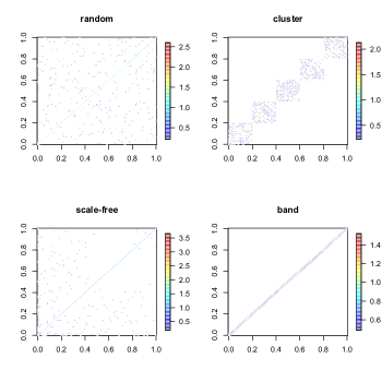
Figure 1: Illustration of the various graph structures of the precision matrix used in our simulation study.

Our experiment is similar to the local basis experiment: the $n$ spatial observation locations are randomly uniformly sampled from the square $[0,\sqrt{n}]\times[0,\sqrt{n}]$ where we entertain $n\in\{100^{2},150^{2},200^{2}\}$ and $\ell\in\{100,225,400\}$. We use the R package huge (Zhao et al., 2015) to randomly generate the four enumerated precision matrices above. Each graph is generated using default parameters. The same test statistics as reported in the previous section, again averaged over 30 trials, are recorded in Tables 3-6.

Table 3: Simulation study results for the Band graphical model. Scores are averaged over 30 independent trials. Each column represents the number of observation samples, number of basis functions, Frobenius norm, KL divergence, percent of true zeros missed, percent of true nonzeros missed, estimated nugget, true nugget, estimated negative log-likelihood and true negative log-likelihood.

$n$	$\ell$	Frob	KL	$\%$MZ	$\%$MNZ	$\hat{\tau}^{2}$	$\tau^{2}$	$f(\hat{Q},\hat{\tau}^{2})$	$f(Q,\tau^{2})$
	100	0.17	1.5	8.5%	0%	5.0	5.0	26853	26854
10000	225	0.19	4.2	4.6%	0%	11.3	11.3	35553	35555
	400	0.21	8.7	2.4%	0%	20.0	20.0	42079	42081
	100	0.17	1.5	8.5%	0%	5.1	5.1	59691	59692
22500	225	0.19	4.2	4.7%	0%	11.3	11.3	78562	78564
	400	0.20	8.6	2.4%	0%	20.1	20.1	92401	92402
	100	0.17	1.5	8.6%	0%	5.0	5.0	105563	105564
40000	225	0.19	4.2	4.7%	0%	11.3	11.3	138598	138600
	400	0.20	8.6	2.4%	0%	20.0	20.0	162575	162576

Table 4: Simulation study results for the Cluster graphical model. Scores are averaged over 30 independent trials. Each column represents the number of observation samples, number of basis functions, Frobenius norm, KL divergence, percent of true zeros missed, percent of true nonzeros missed, estimated nugget, true nugget, estimated negative log-likelihood and true negative log-likelihood.

$n$	$\ell$	Frob	KL	$\%$MZ	$\%$MNZ	$\hat{\tau}^{2}$	$\tau^{2}$	$f(\hat{Q},\hat{\tau}^{2})$	$f(Q,\tau^{2})$
	100	0.26	3.1	16.3%	0%	5.1	5.1	26867	26868
10000	225	0.30	8.9	8.9%	0%	11.3	11.3	35573	35576
	400	0.32	18	5%	0%	20.0	20.0	42115	42118
	100	0.26	3.1	17.1%	0%	5.1	5.1	59690	59691
22500	225	0.29	8.6	9.0%	0%	11.3	11.3	78567	78570
	400	0.31	17.8	5.0%	0%	20.0	20.0	92420	92423
	100	0.26	3.1	17.5%	0%	5.1	5.1	105568	105570
40000	225	0.29	8.7	9.1%	0%	11.3	11.3	138625	138628
	400	0.31	17.6	5.1%	0%	20.0	20.0	162620	162624

Table 5: Simulation study results for the Random graphical model. Scores are averaged over 30 independent trials. Each column represents the number of observation samples, number of basis functions, Frobenius norm, KL divergence, percent of true zeros missed, percent of true nonzeros missed, estimated nugget, true nugget, estimated negative log-likelihood and true negative log-likelihood.

$n$	$\ell$	Frob	KL	$\%$MZ	$\%$MNZ	$\hat{\tau}^{2}$	$\tau^{2}$	$f(\hat{Q},\hat{\tau}^{2})$	$f(Q,\tau^{2})$
	100	0.19	1.7	9.6%	0%	5.1	5.1	26872	26873
10000	225	0.20	4.8	5.2%	0%	11.3	11.3	35586	35589
	400	0.22	9.8	2.6%	0%	20.0	20.0	42134	42136
	100	0.19	1.8	9.7%	0%	5.1	5.1	59697	59698
22500	225	0.20	4.8	5.2%	0%	11.3	11.3	78581	78584
	400	0.22	9.7	2.6%	0%	20.0	20.0	92441	92443
	100	0.19	1.7	9.8%	0%	5.1	5.1	105585	105586
40000	225	0.20	4.7	5.2%	0%	11.3	11.3	138643	138645
	400	0.22	9.7	2.6%	0%	20.0	20.0	162640	162642

Table 6: Simulation study results for the Scale-free graphical model. Scores are averaged over 30 independent trials. Each column represents the number of observation samples, number of basis functions, Frobenius norm, KL divergence, percent of true zeros missed, percent of true nonzeros missed, estimated nugget, true nugget, estimated negative log-likelihood and true negative log-likelihood.

$n$	$\ell$	Frob	KL	$\%$MZ	$\%$MNZ	$\hat{\tau}^{2}$	$\tau^{2}$	$f(\hat{Q},\hat{\tau}^{2})$	$f(Q,\tau^{2})$
	100	0.21	1.4	6.1%	0%	5.1	5.1	26879	26879
10000	225	0.21	3.5	2.8%	0%	11.3	11.3	35604	35605
	400	0.21	6.3	2.6%	0%	20.0	20.0	42167	42172
	100	0.20	1.4	5.9%	0%	5.1	5.1	59698	59699
22500	225	0.21	3.5	2.8%	0%	11.3	11.3	78598	78599
	400	0.21	6.3	2.7%	0%	20.0	20.0	92471	92476
	100	0.20	1.3	6.1%	0%	5.1	5.1	105597	105598
40000	225	0.21	3.5	2.8%	0%	11.3	11.3	138661	138662
	400	0.21	6.2	2.7%	0%	20.0	20.0	162671	162676

3.2.1 Comments

Tables 3, 4, 5, and 6 contain the results of the global basis simulation study. As in the compactly supported basis study we note the same behavior in $\hat{\tau}^{2}$ in that the independent identical coefficient assumption (constant diagonal $Q$) yields robust estimates of $\tau^{2}$. The cluster graph appears highest in Frobenius norm and KL divergence, but this should not be surprising given the fact that there are more nonzero elements in the cluster graph than its counterparts and we are searching for a sparse estimate. The percentage of missed zeros and missed nonzeros in $Q$ also behave similarly to the local basis study with respect to the dimension $\ell$. Overall the proposed method seems to supply reasonable estimates of the zero structure of the precision matrix, as well as its non-zero values.

3.3 Changing the Ensemble Size and the Noise-to-Signal Ratio

We consider a brief study to assess the effect of ensemble size, or field realizations, on the algorithm’s ability to recover $Q$. In the prior section, we fixed the ensemble size at $m=500$. Here we fix $\ell=100$ to ease computation times but vary the ensemble size according to $m\in\{50,100,200,500,1000\}$ and number of spatial locations according to $n\in\{100^{2},150^{2},200^{2},250^{2},300^{2}\}$. The same Wendland basis and precision matrix $Q$ as in the local basis study (3.1) are used to generate $m$ realizations of the additive model (4) where we have observations at $n$ uniformly randomly sampled locations in $[0,1]\times[0,1]$. We record the Frobenius norm $\|\hat{Q}-Q\|_{F}/\|Q\|_{F}$, the KL divergence $\text{tr}(\hat{Q}Q)-\log\det(\hat{Q}Q)-\ell$, and the percentage of zeros in $Q$ that $\hat{Q}$ fails to capture. The penalty parameter is fixed at $\lambda=0.005$, the value which was favored in our previous simulations when $(\ell,m,n)=(100,500,10000)$.

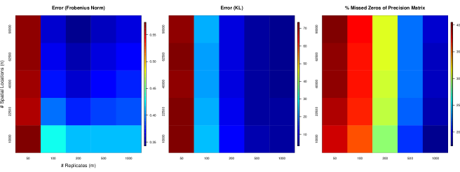
Figure 2: Results of a small simulation study where we fix the basis size $\ell$ but vary sample size $m$ and number of spatial locations $n$. The penalty matrix is fixed across each pair $(n,m)$.

Figure 2 shows results from this study. The plots suggest that the number of replicates $m$ has a prominent effect on our summary statistics, while the influence of the spatial dimension $n$ is more subtle. The Frobenius norm and KL divergence decrease as $n$ increases but much more noticeably decrease when $m$ increases, with the effects less pronounced beyond the $m=50$ range. The percentage of missed zeros in $\hat{Q}$ behaves similarly, but the accuracy does not rise so sharply beyond $m=50$.

We also conducted a small experiment where we changed the noise-to-signal ratio, which has been kept at $0.1$ up to this point, under a fixed set of basis functions and precision matrix $Q$. The penalty matrix was also kept constant across the various noise levels. Increasing the ratio from $0.1$ to $0.25$ slightly worsened the Frobenius norm and KL divergence, but the jump from $0.25$ to $0.5$ demonstrated a substantial decrease in ability to accurately capture the true precision matrix. At a noise-to-signal ratio of 0.5, however, the resulting model is extremely noisy and expecting accurate estimates is not entirely reasonable.

Finally, we note that the estimation procedure for $\hat{\tau}^{2}$ in Section 2.2.1 remained extremely accurate throughout all the modifications in this section.

4 Data Analysis

4.1 Reforecast Data

The Global Ensemble Forecast System (GEFS) from the National Center for Environmental Prediction (NCEP) provides an 11 member daily reforecast of climate variables available from December 1984 to present day. We take all readings from January of each year through 2018, giving a total of $m=1054$ global fields of the two meter temperature variable. Measurements were recorded at each integer valued longitude and latitude combination, totaling $n=65160$ spatial locations. We use a set of Wendland basis functions spread over the globe in a way that ensures that the $\ell=2531$ centers are equispaced with respect to the great circle distance. See Figure 3 for an illustration of the data and basis functions. We opt for 2531 as it provides a reasonably dense network of basis functions that still allows for computational tractability.

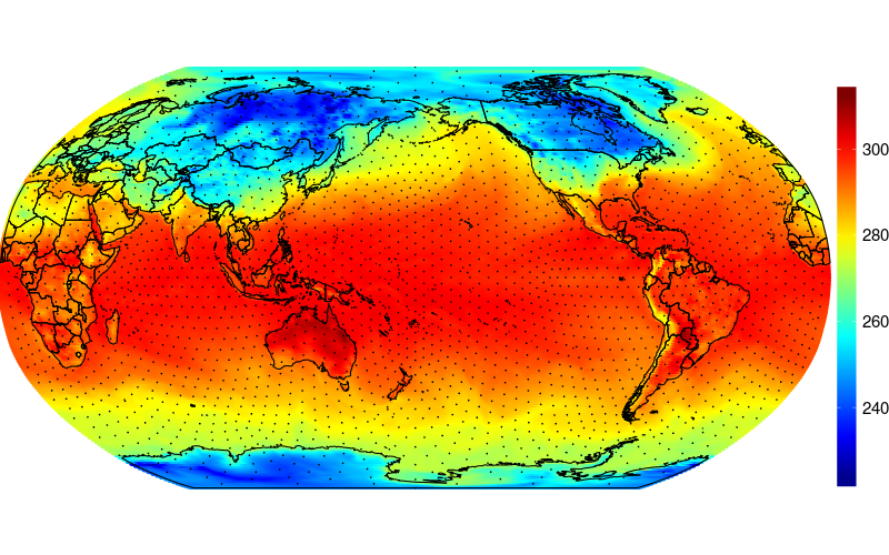
Figure 3: Two meter temperature on January 1, 1984. Dots indicate nodal points.

Throughout this section, we work with temperature anomalies, that is, residuals after removing a spatially-constant mean of approximately 276^∘ K from the data matrix. The technique introduced in Section 2.2.1 is used to estimate the nugget effect $\hat{\tau}^{2}=1.74$.

An interesting idea when using localized basis functions with a notion of distance between them is to adjust the penalty matrix so that neighbors are encouraged to remain in close proximity to the center point. In particular, we make $\Lambda$ proportional to the distance matrix of the centers of the basis functions. This idea was pursued in (Davanloo Tajbakhsh et al., 2014) but in the context of direct spatial observations with the graphical lasso rather than working through basis functions with our DC algorithm.

We consider $\Lambda=\lambda D$ where $D$ is the pairwise distance matrix of the nodal points registering the Wendland basis functions. To select the penalty parameter $\lambda$, we use two-fold likelihood-based cross-validation as described in Section 2.2.2 for values $\lambda\in\{0.0001,0.0005,\linebreak 0.001,0.005,0.01,0.05,0.1,0.5\}$. Smaller values than $0.0001$ were examined but failed to converge after a reasonable runtime. Despite the fact that it sits on the boundary of our parameter set, the value $\lambda=0.0001$ was chosen as at yielded a significant drop in negative log-likelihood when compared to larger penalties. We apply the DC algorithm (11) a final time with the full sample covariance matrix and the $\Lambda$ favored by cross-validation.

Figure 4: Estimated pointwise standard deviations under the model (3) using $Q$ estimated from the DC algorithm. Units are degrees Celsius.

Figure 4 contains a global plot of the implied estimated local standard deviations. Note similar behavior in Figure 4 of Legates and Willmott (1990) which depicts standard deviations for mean air surface temperature over the globe. Both plots illustrate a clear land-ocean difference and increased variability in higher latitudes where the overall land area is greater.

Figure 5 shows a plot of estimated spatial covariance functions centered at three different geographical locations in the southern tip of South America, the Middle East, and central North America. There is clear evidence of nonstationarity in all three cases, as well as negative correlation at medium distances. An interesting feature of the estimated covariance structure is the negative correlation between Alaska and the central United States, indicative of medium-range teleconnections, and may be a result of Rossby waves that occur during winter in the northern hemisphere.

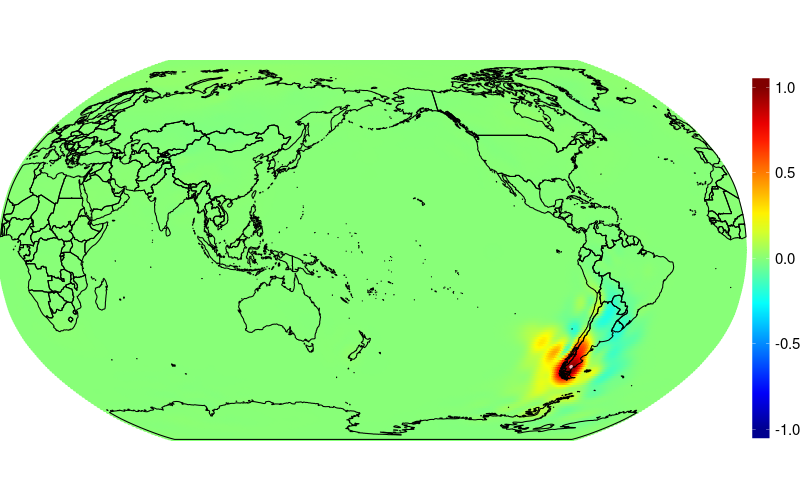
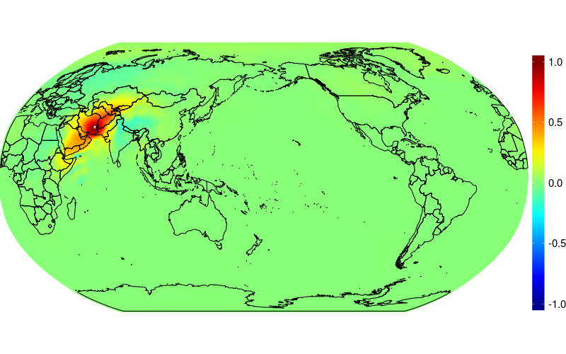
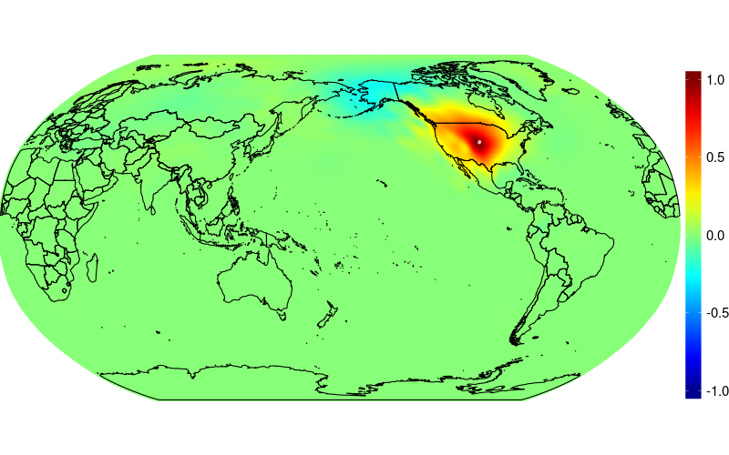
Figure 5: Estimated spatial correlation functions centered at a point in southern South America (left), central Middle East (middle) and central North America (right).

An interesting byproduct of our model is that we can examine the GMRF neighborhood structure of the estimated precision matrix. Recall that each random coefficient $c_{i}$ in our model is registered to a nodal grid shown in Figure 3, and thus we can identify estimated spatial neighborhood patterns according to this grid. We illustrate some of these neighborhood structures, colored by their respective $Q$ values in Figure 6. For nodal points over the ocean, the tendency is large, positive precision values with few neighbors. For nodal points over land, we observe that the most significantly nonzero neighbor elements are geographically near the center node, partly due to our choice for $\Lambda$. There is sometimes evidence of neighborhoods that spread throughout the globe, although the magnitude of the corresponding precision matrix entries is typically very small, e.g., the lower right panel of Figure 6.

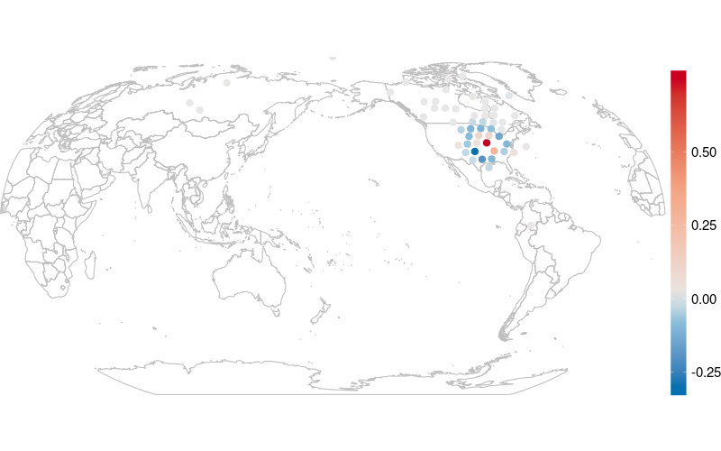
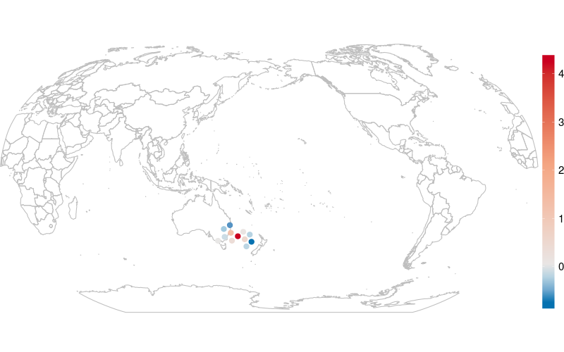
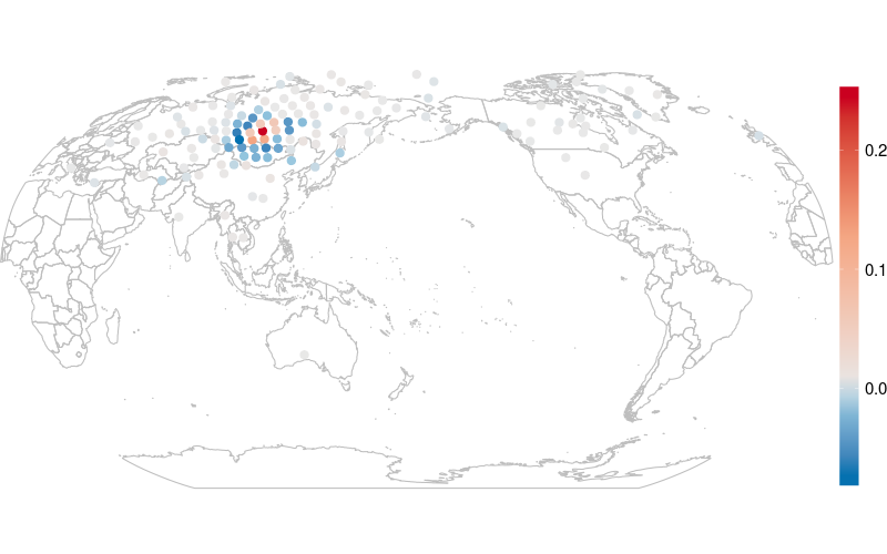
Figure 6: The estimated neighborhood structure of $Q$ registered at the nodal points of the basis functions. Colors correspond to neighborhood entries in $Q$ with a center point that is clockwise starting top left: over U.S.; in Pacific Ocean near Australia; over Russia and over the Pacific Ocean near the equator.

4.2 TopoWx

The Topography Weather (TopoWx) dataset (Oyler et al., 2015) contains observed 2 m temperatures from a set of observation networks over the continental United States. We consider daily minimum temperatures during the month of June from 2010 to 2014, giving a total of $m=150$ replicates. Network locations are chosen to have no missing values, yielding $n=4577$ spatial locations. Figure 7 shows an example day of data on June 1, 2010.

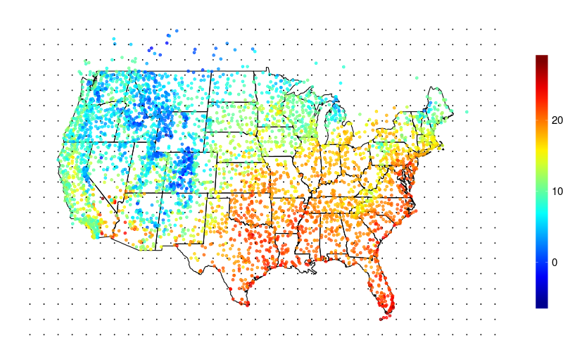
Figure 7: Minimum temperature on June 1, 2010, overlaid with a grid of basis functions nodes.

The dataset includes an elevation covariate, and we work with minimum temperature residuals after regressing out a mean function linear in longitude, latitude and elevation. We transform the raw spatial coordinates with a sinusoidal projection. Our statistical model for the temperature residuals uses Wendland basis functions centered at nodes displayed in Figure 7. We opt for $\ell=1160$ functions using a single level of resolution. The nodal grid and Wendland functions are chosen to match up with a LatticeKrig model specification, but with relaxed assumptions on the precision matrix governing the random coefficients.

The nugget estimate $\hat{\tau}^{2}=2.18$ is retrieved as in Section 2.2.1. As with the previous dataset, the penalty matrix $\Lambda$ is parameterized according to $\Lambda=\lambda D$, where $D$ is the distance matrix of node points. We selected scaling parameters from $\lambda\in\{\frac{1}{10},\frac{2}{10},\dots,\frac{9}{10},1,\frac{10}{9},\dots,\frac{10}{2},10\}\cup\{10,12.5,\dots,27.5,30\}$ using a simple prediction-based cross validation scheme in Section 2.2.2; the latter set in the union was considered to check the behavior of the final estimate $\lambda=10$ near the boundary. The resulting penalty matrix is used with $\hat{\tau}^{2}$ and the full sample covariance $S$ to obtain a final estimate of the precision matrix.

Figures 8 and 9 show graphical model neighborhoods and estimated correlation functions centered at locations in Utah and Kansas. Clear anisotropy and nonstationarity is present in the estimated correlation functions with greater north-south directionality of correlation, while the neighborhood structure for the Utah nodal point displays greater complexity than the relatively nearby neighbors of the nodal point in the midwest.

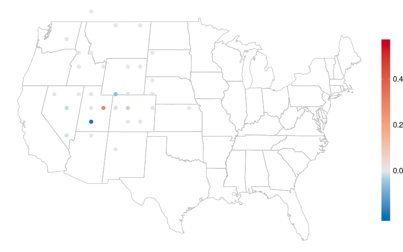
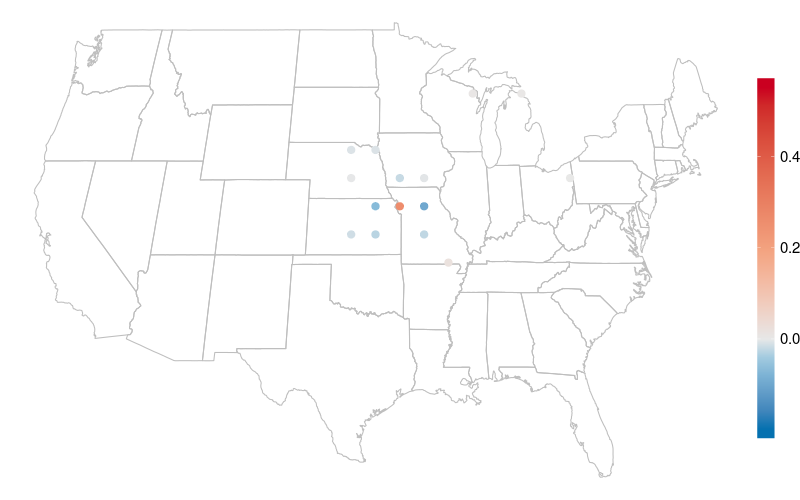
Figure 8: Displaying the neighborhood structure of $Q$, where the two center points are located in central Utah and near Kansas City. Neighbors are colored according to the corresponding nonzero elements in $Q$.

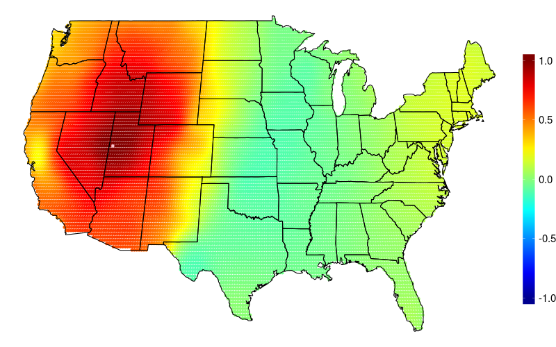
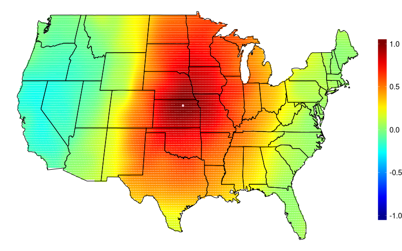
Figure 9: Estimated spatial correlation functions centered at the pink-colored locations in Utah and Kansas.

Due to lack of data availability over the ocean there is an identifiability problem with our method. Since several of the Wendland basis functions lie over the ocean where there is no observed data, we cannot expect the algorithm to give reasonable estimates for the diagonal elements of $Q$ corresponding to those nodes. Moreover, the diagonal of the penalty matrix $\Lambda$ is identically zero, and thus the corresponding diagonal elements of $Q$ remained unchanged no matter the initial guess $Q_{0}$, which we fixed at $Q_{0}=I_{\ell}$.

Now we entertain a comparison against the corresponding LatticeKrig model using the same nodal grid and same Wendland basis functions, but with the spatial autoregressive precision matrix of LatticeKrig. We estimate LatticeKrig parameters by maximum likelihood within the LatticeKrig package in R. In particular, the estimated nugget variance $\hat{\tau}^{2}=4.7$ is about twice as large as that from our model, and the central a.wght parameter is estimated at 5.41. The smoothness parameter $\nu$ in the LatticeKrig setup is set at $0.5$ which is a typical assumption for observational temperature data.

We compare the two models based on cross-validation prediction accuracy and standard Akaike information criterion. For 400 randomly held-out locations, we calculate predictive squared error (MSE) and continuous ranked probability score (CRPS) (Gneiting and Raftery, 2007) based on the standard kriging predictor separately for each of 150 days of data. A nice consequence of the spatial basis model (3) is that the formulas for kriging predictors and kriging variances can be evaluated in $\mathcal{O}(n\ell^{2})$ operations rather than the naive $\mathcal{O}(n^{3})$; see e.g. (Cressie and Johannesson, 2008) for details. The $400\times 150=60000$ MSE and CRPS values are then averaged into single summary statistics. For the proposed model, the MSE and CRPS scores are 4.99 and 3.73, respectively, while the values are 5.02 and 3.64 for LatticeKrig. The similarity of these statistics between models should not come as a surprise given the density of spatial observations.

Direct likelihood comparisons between our proposal and LatticeKrig is not fair due to the high number of free parameters in our model. For spatial processes, the number of degrees of freedom of the model can be identified with the trace of the spatial smoothing hat matrix (Nychka, 2000). Using this estimate of effective degrees of freedom as the number of parameters, our model has AIC of 9043 while LatticeKrig has AIC of 12615, indicating substantial improvement in model fit using our proposal.

4.2.1 Including Global Basis Functions

In the previous section, we removed a mean trend from our data by regressing out longitude, latitude and elevation. Notice, however, that we could simply choose to include for example, elevation, as a global basis function in the stochastic part of the spatial model (3). In light of this viewpoint, we regress out a mean trend on only longitude and latitude and use the same single resolution Wendland basis as before (with $\ell=1160$) but also along with elevation as a global basis function. The penalty matrix $\Lambda$ is selected from a prediction-based cross validation over parameters $(\lambda,\gamma)$, where the upper-left left block of $\Lambda$ reflects distance between the Wendland bases via $\lambda D$, but now the $1161^{st}$ row/column of $\Lambda$ is held at a constant $\gamma$ since there is no natural notion of geographical distance between our global and locally registered basis functions.

By way of illustration, Figure 10 shows estimated spatial correlations using elevation in the stochastic part of the model, which has a noticeable effect. In particular, there are clear estimated spatial correlation patterns with the western point that interact with the nontrivial topography of the western US. The spatial correlation structure in the eastern US is much more homogeneous, reflecting the comparative lack of complex terrain.

An interesting byproduct of including elevation as a globally defined predictor, while the rest of the stochastic basis functions are compactly supported and registered to a grid, is that we can examine the nodal neighbors of the elevation coefficient. To be precise, this corresponds to the first 1160 elements of the $1161^{st}$ row/column of $Q$, as shown in Figure 11. The neighbors, especially those that are substantially different from zero, are concentrated in the western US and over the Appalachian Mountains in the east.

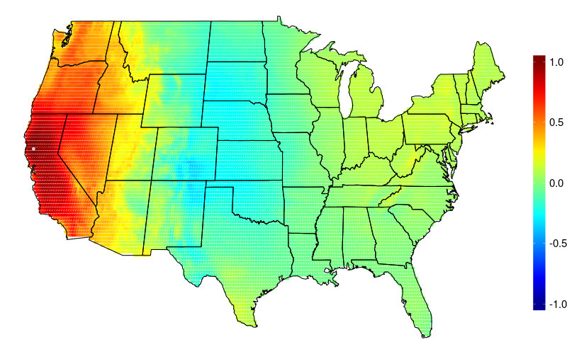
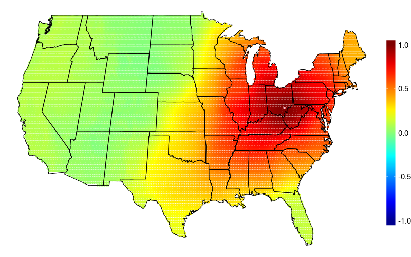
Figure 10: Estimated spatial correlation functions of the process registered at a spatial point colored in pink using elevation as basis function in the stochastic model.

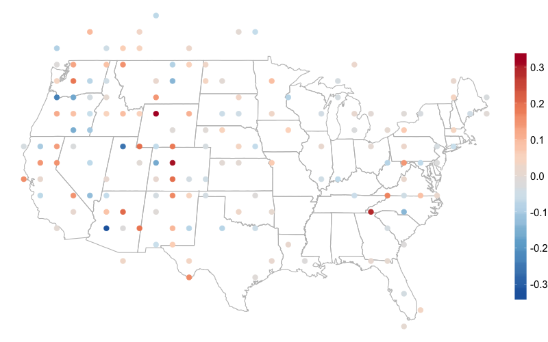
Figure 11: The Wendland coefficient graphical neighbors of the elevation coefficient.

5 Conclusion

In this work we introduce a novel approach for estimating the precision matrix of the random coefficients of a basis representation model that is pervasive in the spatial statistical literature. The only assumption we enforce is that the precision matrix is sparse. In the case that the basis functions are registered to a grid, the precision entries can be interpreted as a spatial Gaussian Markov random field, while graphical model interpretations are still viable with global bases.

The estimator minimizes a penalized log likelihood, and we show that the optimization problem is equivalent to one involving a sum of a convex and concave functions, which suggests a DC-algorithm in which we iteratively linearize the concave part at the previous guess and solve the resulting convex problem. The linearization in our case gives rise to a graphical lasso problem with its “sample covariance” depending upon the previous guess. The graphical lasso problem is well studied and a number of user-friendly R packages exist, headed by the second order method QUIC. Our method has important practical applications in spatial data analysis, since we obtain a nonparametric, penalized maximum likelihood estimate of $Q$ which can subsequently be used in kriging or simulation with computational complexity $\mathcal{O}(n\ell^{2})$ under the basis model.

In our data examples we see that the proposed method performs competitively with existing alternatives such as LatticeKrig, but substantially improves information criteria. Moreover, our model results in highly interpretable fields, allowing for checking of graphical neighborhood structures, or implied nonstationary covariance functions. Future work may be directed toward other penalties, or pushing these notions though to space-time modeling.

6 Appendix

We start the Appendix with the proof of Proposition 1.

Proof of Proposition 1.

For matrices $A,U,C$ and $V$ of appropriate size, the Sherman Woodbury Morrison formula is

$$\left(A+UCV\right)^{-1}=A^{-1}-A^{-1}U\left(C^{-1}+VA^{-1}U\right)^{-1}VA^{-1}$$

and the matrix determinant lemma is

$$\det(A+UCV)=\text{det}(C^{-1}+VA^{-1}U)\ \text{det}(C)\ \text{det}(A).$$

In our case, these two equations read

$$\left(\Phi Q^{-1}\Phi^{\mathrm{T}}+\tau^{2}I_{n}\right)^{-1}=\frac{1}{\tau^{2}}I_{n}-\frac{1}{\tau^{4}}\Phi\left(Q+\frac{1}{\tau^{2}}\Phi^{\mathrm{T}}\Phi\right)^{-1}\Phi^{\mathrm{T}}$$ (16)

and

$$\det(\Phi Q^{-1}\Phi^{\mathrm{T}}+\tau^{2}I_{n})=\det\left(Q+\frac{1}{\tau^{2}}\Phi^{\mathrm{T}}\Phi\right)\det(Q^{-1})\det(\tau^{2}I_{n}).$$ (17)

Combining (16) with linearity and the cyclic property of trace gives

$$\text{tr}(S(\Phi Q^{-1}\Phi^{\mathrm{T}}+\tau^{2}I_{n})^{-1})=\frac{1}{\tau^{2}}\text{tr}(S)-\text{tr}\left(\frac{1}{\tau^{4}}\Phi^{\mathrm{T}}S\Phi\left(Q+\frac{1}{\tau^{2}}\Phi^{\mathrm{T}}\Phi\right)^{-1}\right),$$

and taking the logarithm of (17) immediately yields

$$\log\det(\Phi Q^{-1}\Phi^{\mathrm{T}}+\tau^{2}I_{n})=\log\det\left(Q+\frac{1}{\tau^{2}}\Phi^{\mathrm{T}}\Phi\right)-\log\det Q+n\log\tau^{2}.\hfill\qed$$

Convexity, Gradients, and Hessians

The penalized likelihood in Proposition 1 was as follows:

$$\log\det\left(Q+\frac{1}{\tau^{2}}\Phi^{T}\Phi\right)-\log\det(Q)-\text{tr}\left(\dfrac{1}{\tau^{4}}\Phi^{\mathrm{T}}S\Phi\left(Q+\frac{1}{\tau^{2}}\Phi^{\mathrm{T}}\Phi\right)^{-1}\right)+\|\lambda\circ Q\|_{1}$$

Let us explain the classifications of convexity and concavity stated in the opening paragraph of Section 2.2. The penalty function $Q\mapsto\|\Lambda\circ Q\|_{1}$ is trivially convex on $Q\succeq 0$. An explicit proof of concavity for $Q\mapsto\log\det Q$ on $Q\succeq 0$ is given on page 74 of [Boyd and Vandenberghe, 2004]. The convexity of $\text{tr}(AQ^{-1})$ on $Q\succeq 0$ for an arbitrary positive semidefinite matrix $A$ can be shown in a similar fashion, as the authors suggest in their Exercise 3.18(a). Composition with an affine mapping preserves both convexity and concavity, so $Q\mapsto\log\det\left(Q+\frac{1}{\tau^{2}}\Phi^{\mathrm{T}}\Phi\right)$ is concave on $Q\succeq 0$ and $Q\mapsto\text{tr}\left(A\left(Q+\frac{1}{\tau^{2}}\Phi^{\mathrm{T}}\Phi\right)\right)^{-1}$ is convex on $Q\succeq 0$.

Below we report the gradient and Hessian matrices of the first three terms in this penalized likelihood, with $\otimes$ indicating the Kronecker product of two matrices. Let $W=Q^{-1}$ and $M=\left(Q+\frac{1}{\tau^{2}}\Phi^{\mathrm{T}}\Phi\right)^{-1}$ for shorthand.

$\begin{array}[]{c||c c}\hline\cr\hline\cr&\text{Gradient}&\text{Hessian}\\ \hline\cr\log\det\left(Q+\frac{1}{\tau^{2}}\Phi^{T}\Phi\right)&M&-(M\otimes M)\\[5.0pt] -\log\det(Q)&-W&W\otimes W\\ -\dfrac{1}{\tau^{4}}\text{tr}\left(\Phi^{\mathrm{T}}S\Phi M\right)&\frac{1}{\tau^{4}}M\Phi^{\mathrm{T}}S\Phi M&-\frac{1}{\tau^{4}}\left(M\Phi^{\mathrm{T}}S\Phi M\otimes M\right)-\frac{1}{\tau^{4}}\left(M\otimes M\Phi^{\mathrm{T}}S\Phi M\right)\end{array}$

Our claims of convexity and concavity in the above paragraphs can be further verified with the following fact: if $\{\lambda_{i}\}$ and $\{\mu_{i}\}$ are the eigenvalues of $A$ and $B$, then $A\otimes B$ has eigenvalues $\{\lambda_{i}\mu_{j}\}$ (11.5, [Seber, 2007]).

DC algorithm in R

We provide an algorithm for (11) in R assuming the QUIC package is installed. Mathematical inputs for the algorithm are the nugget effect $\tau^{2}$ and the $\ell\times\ell$ matrices $\Phi^{\mathrm{T}}\Phi$, $\Phi^{\mathrm{T}}S\Phi$, and $\Lambda$.

 

   

 QUIC_DCsolve <- function(lambda,guess,tau_sq,Phi_Phi,Phi_S_Phi,tol,max_iterations,max_runtime_seconds){ 

      norm <- 1 

      counter <- 1 

      Phi_Phi_over_nugget <- Phi_Phi/tau_sq 

      Phi_S_Phi_over_nuggetsq <- Phi_S_Phi / (tau_sq^2) 

      start.time <- Sys.time() 

      elapsed <- 0 

      while (norm >= tol && counter <= max_iterations && elapsed <= max_runtime_seconds) { 

           M <- chol2inv(chol(guess + Phi_Phi_over_nugget)) 

           S_star <- (diag(dim(guess)[1]) + M %*% Phi_S_Phi_over_nuggetsq) %*% M 

           new_guess <- QUIC(S_star,rho=lambda,msg=0)$X 

           current.time <- Sys.time() 

           elapsed <- difftime(current.time,start.time,units="secs") 

           norm <- norm(new_guess - guess,type="F")/norm(guess,type="F") 

           cat("Iteration ", counter, ". Relative error: ", norm, ". Time elapsed: ", elapsed,"\n", sep="") 

           guess <- new_guess 

           counter <- counter+1 

       } 

       if(counter > max_iterations) { 

           cat("Maximum Iterations Reached. Relative error: ", sprintf("%10f",norm), sep ="") 

           cat("\n") 

       } else if(elapsed > max_runtime_seconds) { 

           cat("Maximum run time reached. Relative error: ", sprintf("%10f",norm), sep ="") 

           cat("\n") 

       } else { 

           cat("Convergence. Relative error: ", sprintf("%10f",norm), sep ="") 

           cat("\n") 

           } 

      guess 

 } 

   

 

Alternative DC Algorithm

In the body of this paper, we chose to group the summands of the likelihood (7) individually so that $-\log\det(Q)$ is the only convex term and everything else is concave and hence linearized into the trace term under the DC framework, ultimately giving rise to the graphical lasso subproblem. It is interesting to note that $A\otimes A\succeq B\otimes B\iff A\succeq B$ (11.7, [Seber, 2007]), which, in light of the Hessian calculations shown in the previous section, implies that the entire log determinant contribution

$$\log\det\left(Q+\frac{1}{\tau^{2}}\Phi^{T}\Phi\right)-\log\det(Q)$$

is convex rather than just $-\log\det(Q)$. The DC scheme (9) in this case would read

$$Q_{j+1}=\operatorname*{arg\,min}_{Q\succeq 0}\left(\log\det\left(Q+\frac{1}{\tau^{2}}\Phi^{T}\Phi\right)-\log\det Q+\text{tr}\left(\nabla g(Q_{j})Q\right)+\|\Lambda\circ Q\|_{1}\right)$$ (18)

where now the concave function $g(Q)=-\text{tr}\left(\dfrac{1}{\tau^{4}}\Phi^{\mathrm{T}}S\Phi\left(Q+\frac{1}{\tau^{2}}\Phi^{T}\Phi\right)^{-1}\right)$ is simply the trace term from the likelihood (7). The hope is that linearizing less of the original function at each step may produce a different (better) stationary point, but (18) is an unstudied convex problem and we cannot directly rely on the graphical lasso framework. Fortunately, several concepts from the QUIC algorithm extend directly to the new problem, and a few straightforward modifications to the QUIC source code produces a fast method for (18).

On small, synthetic datasets, the estimated $\hat{Q}$ under the new algorithm (18) and the graphical lasso DC algorithm (11) were indistinguishable, and the latter was faster to reach the strict tolerance $\varepsilon\ll 0.01$. In the case of the real datasets discussed in Section 4, the dimension $\ell$ is large enough so that there is a substantial difference in runtime between the two methods, but again the resulting estimates are essentially the same under a looser tolerance $\varepsilon=0.01$. We therefore chose to motivate our problem in this paper under the graphical lasso DC framework (11), a choice which feels natural given the interpretation of the graphical lasso as estimating the precision matrix in an undirected Gaussian graphical model. Nevertheless, it is interesting to note that that these two DC schemes seem to converge to the same estimate $\hat{Q}$ despite the fact that the original likelihood is not necessarily convex.

References

- Bandyopadhyay and Lahiri [2009] Soutir Bandyopadhyay and Soumendra N. Lahiri. Asymptotic properties of discrete Fourier transforms for spatial data. Sankhyā, 71(2, Ser. A):221–259, 2009. ISSN 0972-7671.
- Banerjee et al. [2008a] Onureena Banerjee, Laurent El Ghaoui, and Alexandre d’Aspremont. Model selection through sparse maximum likelihood estimation for multivariate Gaussian or binary data. J. Mach. Learn. Res., 9:485–516, 2008a. ISSN 1532-4435.
- Banerjee et al. [2008b] Sudipto Banerjee, Alan E. Gelfand, Andrew O. Finley, and Huiyan Sang. Gaussian predictive process models for large spatial data sets. J. R. Stat. Soc. Ser. B Stat. Methodol., 70(4):825–848, 2008b. ISSN 1369-7412. doi: 10.1111/j.1467-9868.2008.00663.x. URL https://doi.org/10.1111/j.1467-9868.2008.00663.x.
- Barabási and Albert [1999] Albert-László Barabási and Réka Albert. Emergence of scaling in random networks. Science, 286(5439):509–512, 1999. ISSN 0036-8075. doi: 10.1126/science.286.5439.509. URL https://doi.org/10.1126/science.286.5439.509.
- Bien and Tibshirani [2011] Jacob Bien and Robert J. Tibshirani. Sparse estimation of a covariance matrix. Biometrika, 98(4):807–820, 2011. ISSN 0006-3444. doi: 10.1093/biomet/asr054. URL https://doi.org/10.1093/biomet/asr054.
- Bolin and Lindgren [2011] David Bolin and Finn Lindgren. Spatial models generated by nested stochastic partial differential equations, with an application to global ozone mapping. Ann. Appl. Stat., 5(1):523–550, 2011. ISSN 1932-6157. doi: 10.1214/10-AOAS383. URL https://doi.org/10.1214/10-AOAS383.
- Boyd and Vandenberghe [2004] Stephen Boyd and Lieven Vandenberghe. Convex optimization, 2004.
- Cressie and Johannesson [2008] Noel Cressie and Gardar Johannesson. Fixed rank kriging for very large spatial data sets. J. R. Stat. Soc. Ser. B Stat. Methodol., 70(1):209–226, 2008. ISSN 1369-7412. doi: 10.1111/j.1467-9868.2007.00633.x. URL https://doi.org/10.1111/j.1467-9868.2007.00633.x.
- Cressie and Wikle [2011] Noel Cressie and Chris Wikle. Statistics for Spatio-Temporal Data. CourseSmart Series. Wiley, 2011. ISBN 9780471692744. URL https://books.google.com/books?id=-kOC6D0DiNYC.
- Davanloo Tajbakhsh et al. [2014] Sam Davanloo Tajbakhsh, Necdet Serhat Aybat, and Enrique Del Castillo. Sparse precision matrix selection for fitting gaussian random field models to large data sets. ArXiv e-prints, May 2014.
- Dinh Tao and Le Thi [1997] Pham Dinh Tao and Hoai An Le Thi. Convex analysis approach to DC programming: Theory, algorithm and applications. Acta Mathematica Vietnamica, 22, 01 1997.
- Fattahi et al. [2019] Salar Fattahi, Richard Y. Zhang, and Somayeh Sojoudi. Linear-time algorithm for learning large-scale sparse graphical models. IEEE Access, pages 1–1, 2019. ISSN 2169-3536. doi: 10.1109/ACCESS.2018.2890583.
- Friedman et al. [2007] Jerome Friedman, Trevor Hastie, Holger Höfling, and Robert Tibshirani. Pathwise coordinate optimization. Ann. Appl. Stat., 1(2):302–332, 2007. ISSN 1932-6157. doi: 10.1214/07-AOAS131. URL https://doi.org/10.1214/07-AOAS131.
- Friedman et al. [2008] Jerome Friedman, Trevor Hastie, and Robert Tibshirani. Sparse inverse covariance estimation with the graphical lasso. Biostatistics, 9(3):432–441, July 2008. ISSN 1465-4644. doi: 10.1093/biostatistics/kxm045. URL https://www.ncbi.nlm.nih.gov/pmc/articles/PMC3019769/.
- Fuentes [2002] Montserrat Fuentes. Spectral methods for nonstationary spatial processes. Biometrika, 89(1):197–210, 2002. ISSN 0006-3444. doi: 10.1093/biomet/89.1.197. URL https://doi.org/10.1093/biomet/89.1.197.
- Gneiting and Raftery [2007] Tilmann Gneiting and Adrian E. Raftery. Strictly proper scoring rules, prediction, and estimation. J. Amer. Statist. Assoc., 102(477):359–378, 2007. ISSN 0162-1459. doi: 10.1198/016214506000001437. URL https://doi.org/10.1198/016214506000001437.
- Guhaniyogi and Banerjee [2018] Rajarshi Guhaniyogi and Sudipto Banerjee. Meta-kriging: scalable Bayesian modeling and inference for massive spatial datasets. Technometrics, 60(4):430–444, 2018. ISSN 0040-1706. doi: 10.1080/00401706.2018.1437474. URL https://doi.org/10.1080/00401706.2018.1437474.
- Hsieh et al. [2014] Cho-Jui Hsieh, Mátyás A. Sustik, Inderjit S. Dhillon, and Pradeep Ravikumar. QUIC: quadratic approximation for sparse inverse covariance estimation. J. Mach. Learn. Res., 15:2911–2947, 2014. ISSN 1532-4435.
- Hunter and Lange [2004] David R. Hunter and Kenneth Lange. A tutorial on MM algorithms. The American Statistician, 58:30–37, 02 2004.
- Katzfuss [2017] Matthias Katzfuss. A multi-resolution approximation for massive spatial datasets. J. Amer. Statist. Assoc., 112(517):201–214, 2017. ISSN 0162-1459. doi: 10.1080/01621459.2015.1123632. URL https://doi.org/10.1080/01621459.2015.1123632.
- Legates and Willmott [1990] David R. Legates and Cort J. Willmott. Mean seasonal and spatial variability in global surface air temperature. Theoretical and Applied Climatology, 41(1):11–21, Mar 1990. ISSN 1434-4483. doi: 10.1007/BF00866198. URL https://doi.org/10.1007/BF00866198.
- Lindgren et al. [2011] Finn Lindgren, Håvard Rue, and Johan Lindström. An explicit link between Gaussian fields and Gaussian Markov random fields: the stochastic partial differential equation approach. J. R. Stat. Soc. Ser. B Stat. Methodol., 73(4):423–498, 2011. ISSN 1369-7412. doi: 10.1111/j.1467-9868.2011.00777.x. URL https://doi.org/10.1111/j.1467-9868.2011.00777.x. With discussion and a reply by the authors.
- Matsuda and Yajima [2009] Yasumasa Matsuda and Yoshihiro Yajima. Fourier analysis of irregularly spaced data on . J. R. Stat. Soc. Ser. B Stat. Methodol., 71(1):191–217, 2009. ISSN 1369-7412. doi: 10.1111/j.1467-9868.2008.00685.x. URL https://doi.org/10.1111/j.1467-9868.2008.00685.x.
- Nychka [2000] Douglas Nychka. Spatial-process estimates as smoothers. In M. G. Schimek, editor, Smoothing and Regression: Approaches, Computation and Application, pages 393–424. New York: Wiley, 2000.
- Nychka et al. [2002] Douglas Nychka, Christopher Wikle, and J. Andrew Royle. Multiresolution models for nonstationary spatial covariance functions. Stat. Model., 2(4):315–331, 2002. ISSN 1471-082X. doi: 10.1191/1471082x02st037oa. URL https://doi.org/10.1191/1471082x02st037oa.
- Nychka et al. [2015] Douglas Nychka, Soutir Bandyopadhyay, Dorit Hammerling, Finn Lindgren, and Stephan Sain. A multiresolution Gaussian process model for the analysis of large spatial datasets. J. Comput. Graph. Statist., 24(2):579–599, 2015. ISSN 1061-8600. doi: 10.1080/10618600.2014.914946. URL https://doi.org/10.1080/10618600.2014.914946.
- Oyler et al. [2015] Jared Wesley Oyler, Ashley Ballantyne, Kelsey Jencso, Michael Sweet, and Steven W. Running. Creating a topoclimatic daily air temperature dataset for the conterminous United States using homogenized station data and remotely sensed land skin temperature. International Journal of Climatology, 35:2258–2279, 2015.
- Roweis and Ghahramani [1999] Sam Roweis and Zoubin Ghahramani. A unifying review of linear gaussian models. Neural computation, 11:305–45, 03 1999.
- Rue and Held [2005] Håvard Rue and Leonhard Held. Gaussian Markov Random Fields: Theory And Applications (Monographs on Statistics and Applied Probability). Chapman & Hall/CRC, 2005. ISBN 1584884320.
- Seber [2007] George A. F. Seber. A Matrix Handbook for Statisticians. Wiley-Interscience, New York, NY, USA, 1st edition, 2007. ISBN 0471748692, 9780471748694.
- Tipping [2001] Michael E. Tipping. Sparse Bayesian learning and the relevance vector machine. J. Mach. Learn. Res., 1(3):211–244, 2001. ISSN 1532-4435. doi: 10.1162/15324430152748236. URL https://doi.org/10.1162/15324430152748236.
- Yuan and Lin [2007] Ming Yuan and Yi Lin. Model selection and estimation in the Gaussian graphical model. Biometrika, 94(1):19–35, 2007. ISSN 0006-3444. doi: 10.1093/biomet/asm018. URL https://doi.org/10.1093/biomet/asm018.
- Zhao et al. [2015] Tuo Zhao, Xingguo Li, Han Liu, Kathryn Roeder, John Lafferty, and Larry Wasserman. huge: High-Dimensional Undirected Graph Estimation, 2015. URL https://CRAN.R-project.org/package=huge. R package version 1.2.7.