Wide Neural Networks of Any Depth Evolve as Linear Models Under Gradient Descent
Abstract
A longstanding goal in deep learning research has been to precisely characterize training and generalization. However, the often complex loss landscapes of neural networks have made a theory of learning dynamics elusive. In this work, we show that for wide neural networks the learning dynamics simplify considerably and that, in the infinite width limit, they are governed by a linear model obtained from the first-order Taylor expansion of the network around its initial parameters. Furthermore, mirroring the correspondence between wide Bayesian neural networks and Gaussian processes, gradient-based training of wide neural networks with a squared loss produces test set predictions drawn from a Gaussian process with a particular compositional kernel. While these theoretical results are only exact in the infinite width limit, we nevertheless find excellent empirical agreement between the predictions of the original network and those of the linearized version even for finite practically-sized networks. This agreement is robust across different architectures, optimization methods, and loss functions.
1 Introduction
Machine learning models based on deep neural networks have achieved unprecedented performance across a wide range of tasks [1, 2, 3]. Typically, these models are regarded as complex systems for which many types of theoretical analyses are intractable. Moreover, characterizing the gradient-based training dynamics of these models is challenging owing to the typically high-dimensional non-convex loss surfaces governing the optimization. As is common in the physical sciences, investigating the extreme limits of such systems can often shed light on these hard problems. For neural networks, one such limit is that of infinite width, which refers either to the number of hidden units in a fully-connected layer or to the number of channels in a convolutional layer. Under this limit, the output of the network at initialization is a draw from a Gaussian process (GP); moreover, the network output remains governed by a GP after exact Bayesian training using squared loss [4, 5, 6, 7, 8]. Aside from its theoretical simplicity, the infinite-width limit is also of practical interest as wider networks have been found to generalize better [5, 7, 9, 10, 11].
In this work, we explore the learning dynamics of wide neural networks under gradient descent and find that the weight-space description of the dynamics becomes surprisingly simple: as the width becomes large, the neural network can be effectively replaced by its first-order Taylor expansion with respect to its parameters at initialization. For this linear model, the dynamics of gradient descent become analytically tractable. While the linearization is only exact in the infinite width limit, we nevertheless find excellent agreement between the predictions of the original network and those of the linearized version even for finite width configurations. The agreement persists across different architectures, optimization methods, and loss functions.
For squared loss, the exact learning dynamics admit a closed-form solution that allows us to characterize the evolution of the predictive distribution in terms of a GP. This result can be thought of as an extension of “sample-then-optimize" posterior sampling [12] to the training of deep neural networks. Our empirical simulations confirm that the result accurately models the variation in predictions across an ensemble of finite-width models with different random initializations.
Here we summarize our contributions:
-
•
Parameter space dynamics: We show that wide network training dynamics in parameter space are equivalent to the training dynamics of a model which is affine in the collection of all network parameters, the weights and biases. This result holds regardless of the choice of loss function. For squared loss, the dynamics admit a closed-form solution as a function of time.
-
•
Sufficient conditions for linearization: We formally prove that there exists a threshold learning rate (see Theorem 2.1), such that gradient descent training trajectories with learning rate smaller than stay in an -neighborhood of the trajectory of the linearized network when , the width of the hidden layers, is sufficiently large.
-
•
Output distribution dynamics: We formally show that the predictions of a neural network throughout gradient descent training are described by a GP as the width goes to infinity (see Theorem 2.2), extending results from Jacot et al. [13]. We further derive explicit time-dependent expressions for the evolution of this GP during training. Finally, we provide a novel interpretation of the result. In particular, it offers a quantitative understanding of the mechanism by which gradient descent differs from Bayesian posterior sampling of the parameters: while both methods generate draws from a GP, gradient descent does not generate samples from the posterior of any probabilistic model.
-
•
Large scale experimental support: We empirically investigate the applicability of the theory in the finite-width setting and find that it gives an accurate characterization of both learning dynamics and posterior function distributions across a variety of conditions, including some practical network architectures such as the wide residual network [14].
-
•
Parameterization independence: We note that linearization result holds both in standard and NTK parameterization (defined in §2.1), while previous work assumed the latter, emphasizing that the effect is due to increase in width rather than the particular parameterization.
-
•
Analytic and neural tangent kernels: We compute the analytic neural tangent kernel corresponding to fully-connected networks with or nonlinearities.
-
•
Source code: Example code investigating both function space and parameter space linearized learning dynamics described in this work is released as open source code within [15].111Note that the open source library has been expanded since initial submission of this work. We also provide accompanying interactive Colab notebooks for both parameter space222colab.sandbox.google.com/github/google/neural-tangents/blob/master/notebooks/weight_space_linearization.ipynb and function space333colab.sandbox.google.com/github/google/neural-tangents/blob/master/notebooks/function_space_linearization.ipynb linearization.
1.1 Related work
We build on recent work by Jacot et al. [13] that characterize the exact dynamics of network outputs throughout gradient descent training in the infinite width limit. Their results establish that full batch gradient descent in parameter space corresponds to kernel gradient descent in function space with respect to a new kernel, the Neural Tangent Kernel (NTK). We examine what this implies about dynamics in parameter space, where training updates are actually made.
Daniely et al. [16] study the relationship between neural networks and kernels at initialization. They bound the difference between the infinite width kernel and the empirical kernel at finite width , which diminishes as . Daniely [17] uses the same kernel perspective to study stochastic gradient descent (SGD) training of neural networks.
Saxe et al. [18] study the training dynamics of deep linear networks, in which the nonlinearities are treated as identity functions. Deep linear networks are linear in their inputs, but not in their parameters. In contrast, we show that the outputs of sufficiently wide neural networks are linear in the updates to their parameters during gradient descent, but not usually their inputs.
Du et al. [19], Allen-Zhu et al. [20, 21], Zou et al. [22] study the convergence of gradient descent to global minima. They proved that for i.i.d. Gaussian initialization, the parameters of sufficiently wide networks move little from their initial values during SGD. This small motion of the parameters is crucial to the effect we present, where wide neural networks behave linearly in terms of their parameters throughout training.
Mei et al. [23], Chizat and Bach [24], Rotskoff and Vanden-Eijnden [25], Sirignano and Spiliopoulos [26] analyze the mean field SGD dynamics of training neural networks in the large-width limit. Their mean field analysis describes distributional dynamics of network parameters via a PDE. However, their analysis is restricted to one hidden layer networks with a scaling limit different from ours , which is commonly used in modern networks [2, 27].
Chizat et al. [28]444We note that this is a concurrent work and an expanded version of this note is presented in parallel at NeurIPS 2019. argued that infinite width networks are in ‘lazy training’ regime and maybe too simple to be applicable to realistic neural networks. Nonetheless, we empirically investigate the applicability of the theory in the finite-width setting and find that it gives an accurate characterization of both the learning dynamics and posterior function distributions across a variety of conditions, including some practical network architectures such as the wide residual network [14].
2 Theoretical results
2.1 Notation and setup for architecture and training dynamics
Let denote the training set and and denote the inputs and labels, respectively. Consider a fully-connected feed-forward network with hidden layers with widths , for and a readout layer with . For each , we use to represent the pre- and post-activation functions at layer with input . The recurrence relation for a feed-forward network is defined as
| (1) |
where is a point-wise activation function, and are the weights and biases, and are the trainable variables, drawn i.i.d. from a standard Gaussian at initialization, and and are weight and bias variances. Note that this parametrization is non-standard, and we will refer to it as the NTK parameterization. It has already been adopted in several recent works [29, 30, 13, 19, 31]. Unlike the standard parameterization that only normalizes the forward dynamics of the network, the NTK-parameterization also normalizes its backward dynamics. We note that the predictions and training dynamics of NTK-parameterized networks are identical to those of standard networks, up to a width-dependent scaling factor in the learning rate for each parameter tensor. As we derive, and support experimentally, in Supplementary Material (SM) §F and §G, our results (linearity in weights, GP predictions) also hold for networks with a standard parameterization.
We define , the vector of all parameters for layer . then indicates the vector of all network parameters, with similar definitions for and . Denote by the time-dependence of the parameters and by their initial values. We use to denote the output (or logits) of the neural network at time . Let denote the loss function where the first argument is the prediction and the second argument the true label. In supervised learning, one is interested in learning a that minimizes the empirical loss555To simplify the notation for later equations, we use the total loss here instead of the average loss, but for all plots in §3, we show the average loss.,
Let be the learning rate666Note that compared to the conventional parameterization, is larger by factor of width [31]. The NTK parameterization allows usage of a universal learning rate scale irrespective of network width.. Via continuous time gradient descent, the evolution of the parameters and the logits can be written as
| (2) | ||||
| (3) |
where , the vector of concatenated logits for all examples, and is the gradient of the loss with respect to the model’s output, . is the tangent kernel at time , which is a matrix
| (4) |
One can define the tangent kernel for general arguments, e.g. where is test input. At finite-width, will depend on the specific random draw of the parameters and in this context we refer to it as the empirical tangent kernel.
The dynamics of discrete gradient descent can be obtained by replacing and with and above, and replacing with below.
2.2 Linearized networks have closed form training dynamics for parameters and outputs
In this section, we consider the training dynamics of the linearized network. Specifically, we replace the outputs of the neural network by their first order Taylor expansion,
| (5) |
where is the change in the parameters from their initial values. Note that is the sum of two terms: the first term is the initial output of the network, which remains unchanged during training, and the second term captures the change to the initial value during training. The dynamics of gradient flow using this linearized function are governed by,
| (6) | |||
| (7) |
As remains constant throughout training, these dynamics are often quite simple. In the case of an MSE loss, i.e., , the ODEs have closed form solutions
| (8) | |||
| (9) |
For an arbitrary point , , where
| (10) | ||||
| (11) |
Therefore, we can obtain the time evolution of the linearized neural network without running gradient descent. We only need to compute the tangent kernel and the outputs at initialization and use Equations 8, 10, and 11 to compute the dynamics of the weights and the outputs.
2.3 Infinite width limit yields a Gaussian process
As the width of the hidden layers approaches infinity, the Central Limit Theorem (CLT) implies that the outputs at initialization converge to a multivariate Gaussian in distribution. Informally, this occurs because the pre-activations at each layer are a sum of Gaussian random variables (the weights and bias), and thus become a Gaussian random variable themselves. See [32, 33, 5, 34, 35] for more details, and [36, 7] for a formal treatment.
Therefore, randomly initialized neural networks are in correspondence with a certain class of GPs (hereinafter referred to as NNGPs), which facilitates a fully Bayesian treatment of neural networks [5, 6]. More precisely, let denote the -th output dimension and denote the sample-to-sample kernel function (of the pre-activation) of the outputs in the infinite width setting,
| (12) |
then , where denotes the covariance between the -th output of and -th output of , which can be computed recursively (see Lee et al. [5, §2.3] and SM §E). For a test input , the joint output distribution is also multivariate Gaussian. Conditioning on the training samples777 This imposes that directly corresponds to the network predictions. In the case of softmax readout, variational or sampling methods are required to marginalize over . , , the distribution of is also a Gaussian ,
| (13) |
and where . This is the posterior predictive distribution resulting from exact Bayesian inference in an infinitely wide neural network.
2.3.1 Gaussian processes from gradient descent training
If we freeze the variables after initialization and only optimize , the original network and its linearization are identical. Letting the width approach infinity, this particular tangent kernel will converge to in probability and Equation 10 will converge to the posterior Equation 13 as (for further details see SM §D). This is a realization of the “sample-then-optimize" approach for evaluating the posterior of a Gaussian process proposed in Matthews et al. [12].
If none of the variables are frozen, in the infinite width setting, also converges in probability to a deterministic kernel [13, 37], which we sometimes refer to as the analytic kernel, and which can also be computed recursively (see SM §E). For and nonlinearity, can be exactly computed (SM §C) which we use in §3. Letting the width go to infinity, for any , the output of the linearized network is also Gaussian distributed because Equations 10 and 11 describe an affine transform of the Gaussian . Therefore
Corollary 1.
For every test points in , and , converges in distribution as width goes to infinity to a Gaussian with mean and covariance given by888Here “+h.c.” is an abbreviation for “plus the Hermitian conjugate”.
| (14) | |||
| (15) |
Therefore, over random initialization, has distribution
| (16) |
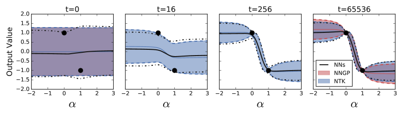
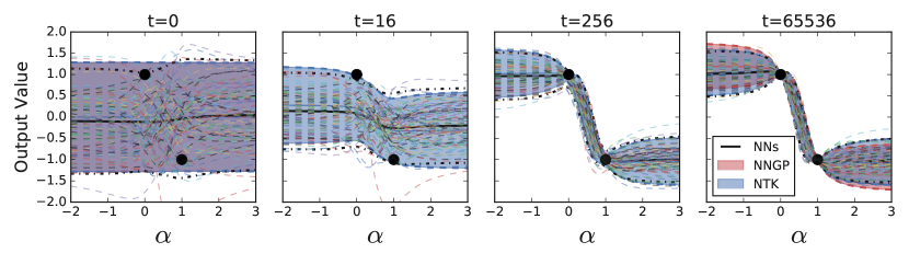
Unlike the case when only is optimized, Equations 14 and 15 do not admit an interpretation corresponding to the posterior sampling of a probabilistic model.999One possible exception is when the NNGP kernel and NTK are the same up to a scalar multiplication. This is the case when the activation function is the identity function and there is no bias term. We contrast the predictive distributions from the NNGP, NTK-GP (i.e. Equations 14 and 15) and ensembles of NNs in Figure 2.
Infinitely-wide neural networks open up ways to study deep neural networks both under fully Bayesian training through the Gaussian process correspondence, and under GD training through the linearization perspective. The resulting distributions over functions are inconsistent (the distribution resulting from GD training does not generally correspond to a Bayesian posterior). We believe understanding the biases over learned functions induced by different training schemes and architectures is a fascinating avenue for future work.
2.4 Infinite width networks are linearized networks
Equation 2 and 3 of the original network are intractable in general, since evolves with time. However, for the mean squared loss, we are able to prove formally that, as long as the learning rate , where is the min/max eigenvalue of , the gradient descent dynamics of the original neural network falls into its linearized dynamics regime.
Theorem 2.1 (Informal).
Let and assume . Applying gradient descent with learning rate (or gradient flow), for every with , with probability arbitrarily close to 1 over random initialization,
| (17) |
Therefore, as , the distributions of and become the same. Coupling with Corollary 1, we have
Theorem 2.2.
We refer the readers to Figure 2 for empirical verification of this theorem. The proof of Theorem 2.1 consists of two steps. The first step is to prove the global convergence of overparameterized neural networks [19, 20, 21, 22] and stability of the NTK under gradient descent (and gradient flow); see SM §G. This stability was first observed and proved in [13] in the gradient flow and sequential limit (i.e. letting , …, sequentially) setting under certain assumptions about global convergence of gradient flow. In §G, we show how to use the NTK to provide a self-contained (and cleaner) proof of such global convergence and the stability of NTK simultaneously. The second step is to couple the stability of NTK with Grönwall’s type arguments [38] to upper bound the discrepancy between and , i.e. the first norm in Equation 17. Intuitively, the ODE of the original network (Equation 3) can be considered as a -fluctuation from the linearized ODE (Equation 7). One expects the difference between the solutions of these two ODEs to be upper bounded by some functional of ; see SM §H. Therefore, for a large width network, the training dynamics can be well approximated by linearized dynamics.
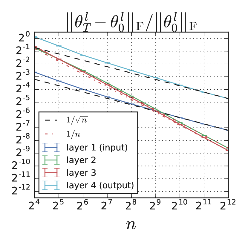

Note that the updates for individual weights in Equation 6 vanish in the infinite width limit, which for instance can be seen from the explicit width dependence of the gradients in the NTK parameterization. Individual weights move by a vanishingly small amount for wide networks in this regime of dynamics, as do hidden layer activations, but they collectively conspire to provide a finite change in the final output of the network, as is necessary for training. An additional insight gained from linearization of the network is that the individual instance dynamics derived in [13] can be viewed as a random features method,101010We thank Alex Alemi for pointing out a subtlety on correspondence to a random features method. where the features are the gradients of the model with respect to its weights.
2.5 Extensions to other optimizers, architectures, and losses
Our theoretical analysis thus far has focused on fully-connected single-output architectures trained by full batch gradient descent. In SM §B we derive corresponding results for: networks with multi-dimensional outputs, training against a cross entropy loss, and gradient descent with momentum.
In addition to these generalizations, there is good reason to suspect the results to extend to much broader class of models and optimization procedures. In particular, a wealth of recent literature suggests that the mean field theory governing the wide network limit of fully-connected models [32, 33] extends naturally to residual networks [35], CNNs [34], RNNs [39], batch normalization [40], and to broad architectures [37]. We postpone the development of these additional theoretical extensions in favor of an empirical investigation of linearization for a variety of architectures.
3 Experiments
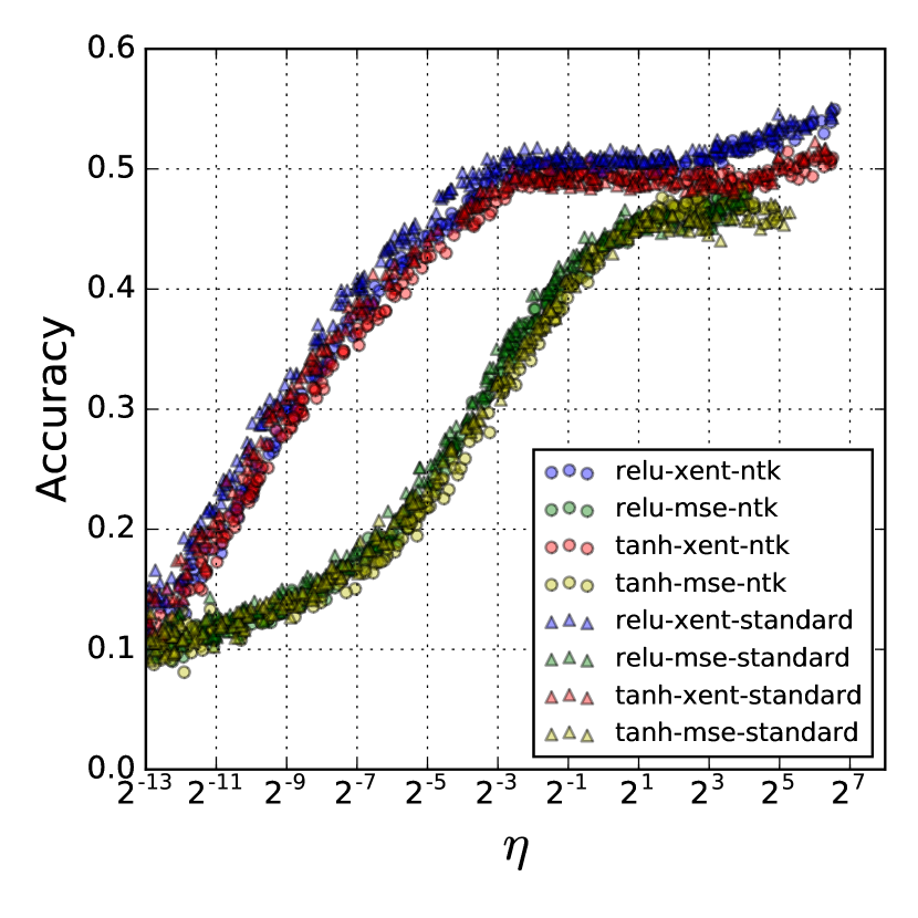
In this section, we provide empirical support showing that the training dynamics of wide neural networks are well captured by linearized models. We consider fully-connected, convolutional, and wide ResNet architectures trained with full- and mini- batch gradient descent using learning rates sufficiently small so that the continuous time approximation holds well. We consider two-class classification on CIFAR-10 (horses and planes) as well as ten-class classification on MNIST and CIFAR-10. When using MSE loss, we treat the binary classification task as regression with one class regressing to and the other to .
Experiments in Figures 1, 4, S2, S3, S4, S5 and S6, were done in JAX [41]. The remaining experiments used TensorFlow [42]. An open source implementation of this work providing tools to investigate linearized learning dynamics is available at www.github.com/google/neural-tangents [15].
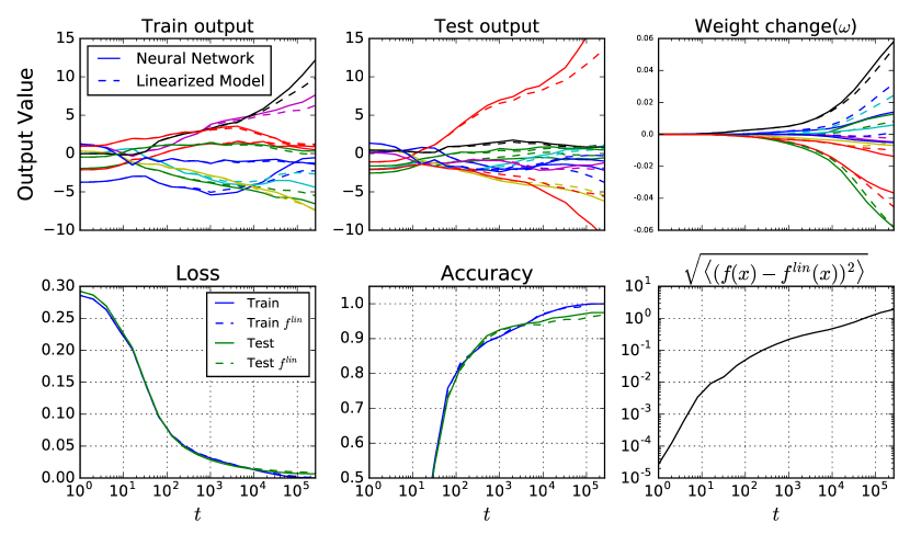
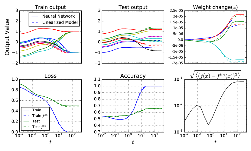
Predictive output distribution: In the case of an MSE loss, the output distribution remains Gaussian throughout training. In Figure 2, the predictive output distribution for input points interpolated between two training points is shown for an ensemble of neural networks and their corresponding GPs. The interpolation is given by where are two training inputs with different classes. We observe that the mean and variance dynamics of neural network outputs during gradient descent training follow the analytic dynamics from linearization well (Equations 14, 15). Moreover the NNGP predictive distribution which corresponds to exact Bayesian inference, while similar, is noticeably different from the predictive distribution at the end of gradient descent training. For dynamics for individual function draws see SM Figure S1.
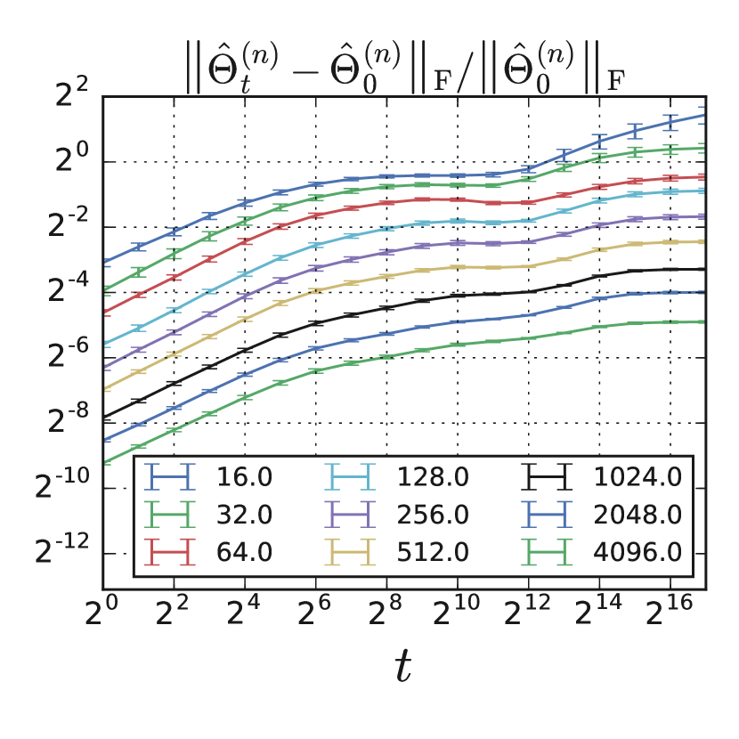
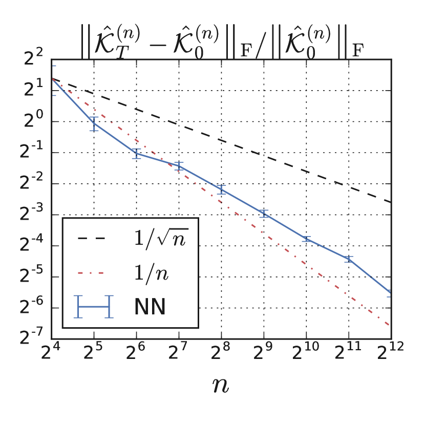
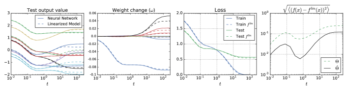
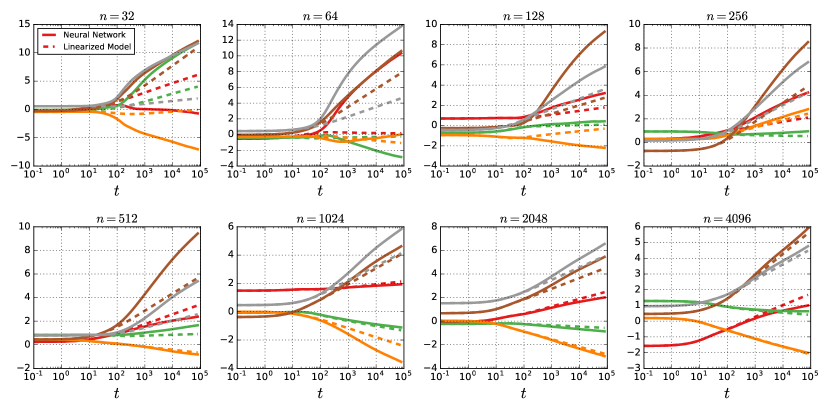
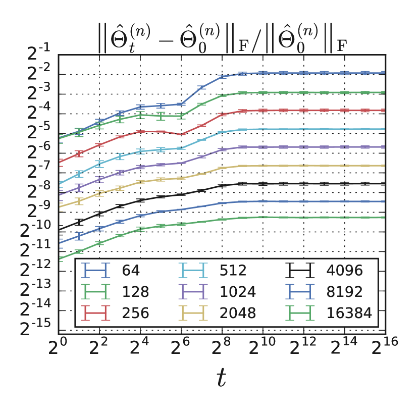
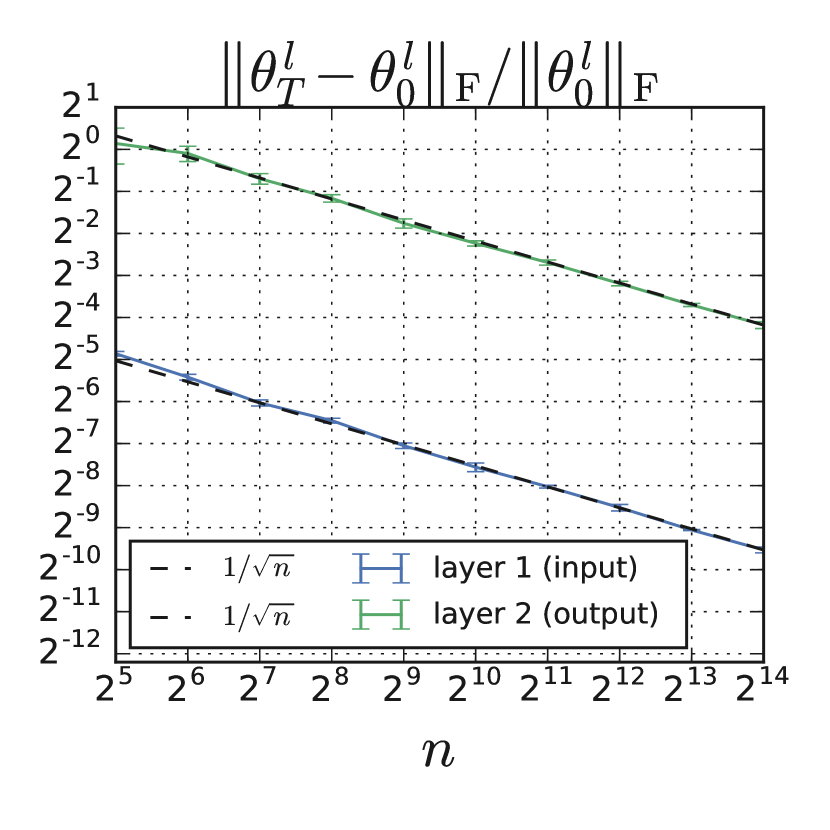
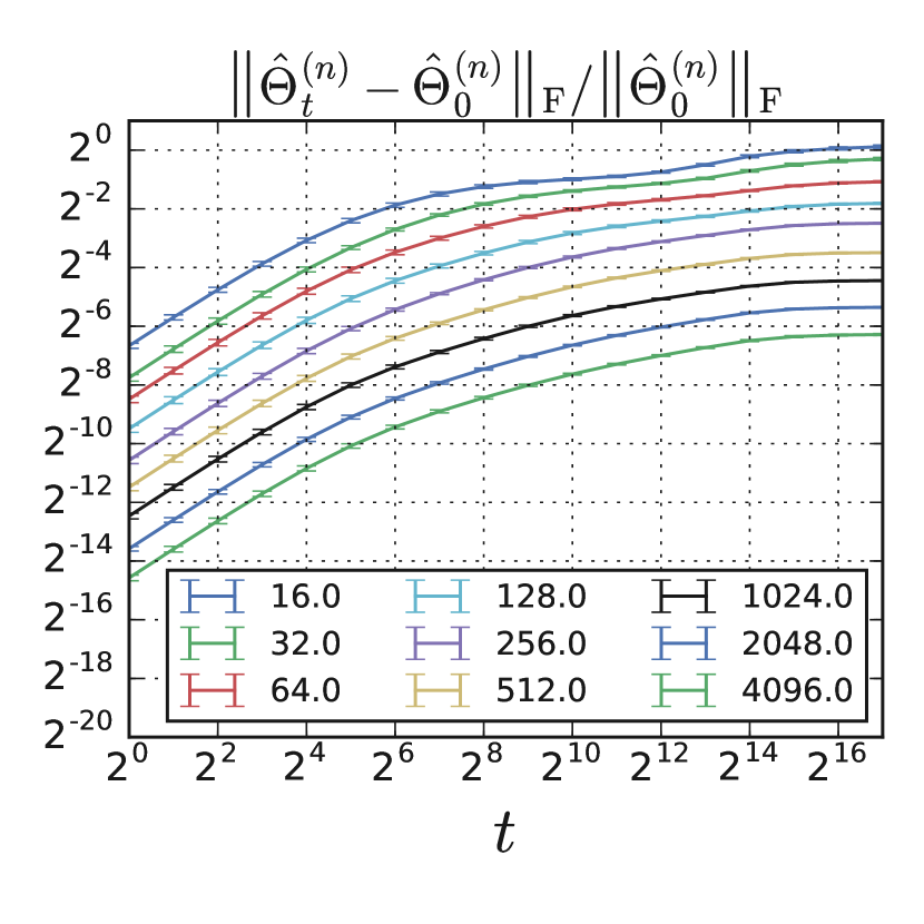
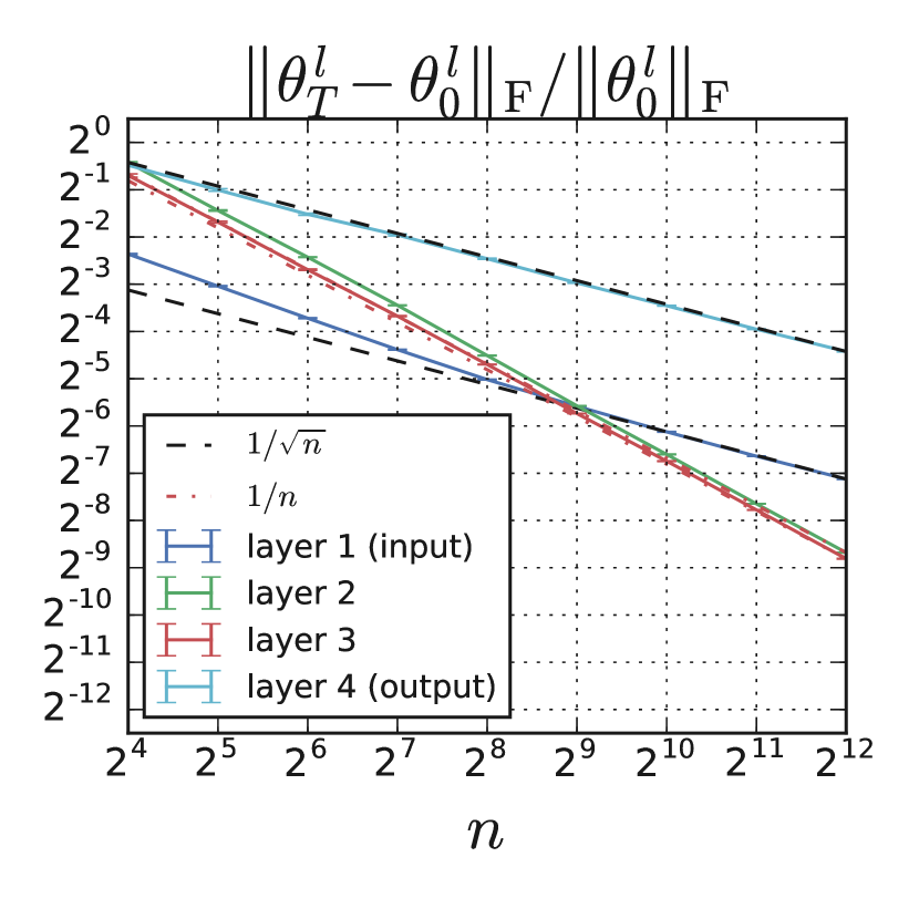
Comparison of training dynamics of linearized network to original network: For a particular realization of a finite width network, one can analytically predict the dynamics of the weights and outputs over the course of training using the empirical tangent kernel at initialization. In Figures 3, 4 (see also S2, S3), we compare these linearized dynamics (Equations 8, 9) with the result of training the actual network. In all cases we see remarkably good agreement. We also observe that for finite networks, dynamics predicted using the empirical kernel better match the data than those obtained using the infinite-width, analytic, kernel . To understand this we note that , where denotes the empirical tangent kernel of width network, as plotted in Figure 1.
One can directly optimize parameters of instead of solving the ODE induced by the tangent kernel . Standard neural network optimization techniques such as mini-batching, weight decay, and data augmentation can be directly applied. In Figure 4 (S2, S3), we compared the training dynamics of the linearized and original network while directly training both networks.
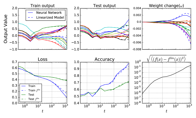
With direct optimization of linearized model, we tested full () MNIST digit classification with cross-entropy loss, and trained with a momentum optimizer (Figure S3). For cross-entropy loss with softmax output, some logits at late times grow indefinitely, in contrast to MSE loss where logits converge to target value. The error between original and linearized model for cross entropy loss becomes much worse at late times if the two models deviate significantly before the logits enter their late-time steady-growth regime (See Figure S4).
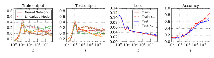
Linearized dynamics successfully describes the training of networks beyond vanilla fully-connected models. To demonstrate the generality of this procedure we show we can predict the learning dynamics of subclass of Wide Residual Networks (WRNs) [14]. WRNs are a class of model that are popular in computer vision and leverage convolutions, batch normalization, skip connections, and average pooling. In Figure 4, we show a comparison between the linearized dynamics and the true dynamics for a wide residual network trained with MSE loss and SGD with momentum, trained on the full CIFAR-10 dataset. We slightly modified the block structure described in Table S1 so that each layer has a constant number of channels (1024 in this case), and otherwise followed the original implementation. As elsewhere, we see strong agreement between the predicted dynamics and the result of training.
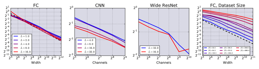
Effects of dataset size: The training dynamics of a neural network match those of its linearization when the width is infinite and the dataset is finite. In previous experiments, we chose sufficiently wide networks to achieve small error between neural networks and their linearization for smaller datasets. Overall, we observe that as the width grows the error decreases (Figure S5). Additionally, we see that the error grows in the size of the dataset. Thus, although error grows with dataset this can be counterbalanced by a corresponding increase in the model size.
4 Discussion
We showed theoretically that the learning dynamics in parameter space of deep nonlinear neural networks are exactly described by a linearized model in the infinite width limit. Empirical investigation revealed that this agrees well with actual training dynamics and predictive distributions across fully-connected, convolutional, and even wide residual network architectures, as well as with different optimizers (gradient descent, momentum, mini-batching) and loss functions (MSE, cross-entropy). Our results suggest that a surprising number of realistic neural networks may be operating in the regime we studied. This is further consistent with recent experimental work showing that neural networks are often robust to re-initialization but not re-randomization of layers (Zhang et al. [43]).
In the regime we study, since the learning dynamics are fully captured by the kernel and the target signal, studying the properties of to determine trainability and generalization are interesting future directions. Furthermore, the infinite width limit gives us a simple characterization of both gradient descent and Bayesian inference. By studying properties of the NNGP kernel and the tangent kernel , we may shed light on the inductive bias of gradient descent.
Some layers of modern neural networks may be operating far from the linearized regime. Preliminary observations in Lee et al. [5] showed that wide neural networks trained with SGD perform similarly to the corresponding GPs as width increase, while GPs still outperform trained neural networks for both small and large dataset size. Furthermore, in Novak et al. [7], it is shown that the comparison of performance between finite- and infinite-width networks is highly architecture-dependent. In particular, it was found that infinite-width networks perform as well as or better than their finite-width counterparts for many fully-connected or locally-connected architectures. However, the opposite was found in the case of convolutional networks without pooling. It is still an open research question to determine the main factors that determine these performance gaps. We believe that examining the behavior of infinitely wide networks provides a strong basis from which to build up a systematic understanding of finite-width networks (and/or networks trained with large learning rates).
Acknowledgements
We thank Greg Yang and Alex Alemi for useful discussions and feedback. We are grateful to Daniel Freeman, Alex Irpan and anonymous reviewers for providing valuable feedbacks on the draft. We thank the JAX team for developing a language which makes model linearization and NTK computation straightforward. We would like to especially thank Matthew Johnson for support and debugging help.
References
- Krizhevsky et al. [2012] Alex Krizhevsky, Ilya Sutskever, and Geoffrey E Hinton. Imagenet classification with deep convolutional neural networks. In Advances in Neural Information Processing Systems. 2012.
- He et al. [2016] Kaiming He, Xiangyu Zhang, Shaoqing Ren, and Jian Sun. Deep residual learning for image recognition. In Conference on Computer Vision and Pattern Recognition, pages 770–778, 2016.
- Devlin et al. [2018] Jacob Devlin, Ming-Wei Chang, Kenton Lee, and Kristina Toutanova. Bert: Pre-training of deep bidirectional transformers for language understanding. arXiv preprint arXiv:1810.04805, 2018.
- Neal [1994] Radford M. Neal. Priors for infinite networks (tech. rep. no. crg-tr-94-1). University of Toronto, 1994.
- Lee et al. [2018] Jaehoon Lee, Yasaman Bahri, Roman Novak, Sam Schoenholz, Jeffrey Pennington, and Jascha Sohl-dickstein. Deep neural networks as gaussian processes. In International Conference on Learning Representations, 2018.
- Matthews et al. [2018a] Alexander G. de G. Matthews, Jiri Hron, Mark Rowland, Richard E. Turner, and Zoubin Ghahramani. Gaussian process behaviour in wide deep neural networks. In International Conference on Learning Representations, 4 2018a. URL https://openreview.net/forum?id=H1-nGgWC-.
- Novak et al. [2019a] Roman Novak, Lechao Xiao, Jaehoon Lee, Yasaman Bahri, Greg Yang, Jiri Hron, Daniel A. Abolafia, Jeffrey Pennington, and Jascha Sohl-Dickstein. Bayesian deep convolutional networks with many channels are gaussian processes. In International Conference on Learning Representations, 2019a.
- Garriga-Alonso et al. [2019] Adrià Garriga-Alonso, Laurence Aitchison, and Carl Edward Rasmussen. Deep convolutional networks as shallow gaussian processes. In International Conference on Learning Representations, 2019.
- Neyshabur et al. [2015] Behnam Neyshabur, Ryota Tomioka, and Nathan Srebro. In search of the real inductive bias: On the role of implicit regularization in deep learning. In International Conference on Learning Representations workshop track, 2015.
- Novak et al. [2018] Roman Novak, Yasaman Bahri, Daniel A. Abolafia, Jeffrey Pennington, and Jascha Sohl-Dickstein. Sensitivity and generalization in neural networks: an empirical study. In International Conference on Learning Representations, 2018.
- Neyshabur et al. [2019] Behnam Neyshabur, Zhiyuan Li, Srinadh Bhojanapalli, Yann LeCun, and Nathan Srebro. The role of over-parametrization in generalization of neural networks. In International Conference on Learning Representations, 2019.
- Matthews et al. [2017] Alexander G. de G. Matthews, Jiri Hron, Richard E. Turner, and Zoubin Ghahramani. Sample-then-optimize posterior sampling for bayesian linear models. In NeurIPS Workshop on Advances in Approximate Bayesian Inference, 2017. URL http://approximateinference.org/2017/accepted/MatthewsEtAl2017.pdf.
- Jacot et al. [2018] Arthur Jacot, Franck Gabriel, and Clement Hongler. Neural tangent kernel: Convergence and generalization in neural networks. In Advances in Neural Information Processing Systems, 2018.
- Zagoruyko and Komodakis [2016] Sergey Zagoruyko and Nikos Komodakis. Wide residual networks. In British Machine Vision Conference, 2016.
- Novak et al. [2019b] Roman Novak, Lechao Xiao, Jiri Hron, Jaehoon Lee, Alexander A. Alemi, Jascha Sohl-Dickstein, and Samuel S. Schoenholz. Neural tangents: Fast and easy infinite neural networks in python. https://github.com/google/neural-tangents, https://arxiv.org/abs/1912.02803, 2019b.
- Daniely et al. [2016] Amit Daniely, Roy Frostig, and Yoram Singer. Toward deeper understanding of neural networks: The power of initialization and a dual view on expressivity. In Advances In Neural Information Processing Systems, 2016.
- Daniely [2017] Amit Daniely. SGD learns the conjugate kernel class of the network. In Advances in Neural Information Processing Systems, 2017.
- Saxe et al. [2014] Andrew M Saxe, James L McClelland, and Surya Ganguli. Exact solutions to the nonlinear dynamics of learning in deep linear neural networks. In International Conference on Learning Representations, 2014.
- Du et al. [2019] Simon S Du, Jason D Lee, Haochuan Li, Liwei Wang, and Xiyu Zhai. Gradient descent finds global minima of deep neural networks. In International Conference on Machine Learning, 2019.
- Allen-Zhu et al. [2019] Zeyuan Allen-Zhu, Yuanzhi Li, and Zhao Song. A convergence theory for deep learning via over-parameterization. In International Conference on Machine Learning, 2019.
- Allen-Zhu et al. [2018] Zeyuan Allen-Zhu, Yuanzhi Li, and Zhao Song. On the convergence rate of training recurrent neural networks. arXiv preprint arXiv:1810.12065, 2018.
- Zou et al. [2019] Difan Zou, Yuan Cao, Dongruo Zhou, and Quanquan Gu. Stochastic gradient descent optimizes over-parameterized deep relu networks. Machine Learning, 2019.
- Mei et al. [2018] Song Mei, Andrea Montanari, and Phan-Minh Nguyen. A mean field view of the landscape of two-layer neural networks. Proceedings of the National Academy of Sciences, 115(33):E7665–E7671, 2018.
- Chizat and Bach [2018] Lenaic Chizat and Francis Bach. On the global convergence of gradient descent for over-parameterized models using optimal transport. In Advances in neural information processing systems, 2018.
- Rotskoff and Vanden-Eijnden [2018] Grant M Rotskoff and Eric Vanden-Eijnden. Parameters as interacting particles: long time convergence and asymptotic error scaling of neural networks. In Advances in neural information processing systems, 2018.
- Sirignano and Spiliopoulos [2018] Justin Sirignano and Konstantinos Spiliopoulos. Mean field analysis of neural networks. arXiv preprint arXiv:1805.01053, 2018.
- Glorot and Bengio [2010] Xavier Glorot and Yoshua Bengio. Understanding the difficulty of training deep feedforward neural networks. In International Conference on Artificial Intelligence and Statistics, pages 249–256, 2010.
- Chizat et al. [2018] Lenaic Chizat, Edouard Oyallon, and Francis Bach. On lazy training in differentiable programming. arXiv preprint arXiv:1812.07956, 2018.
- van Laarhoven [2017] Twan van Laarhoven. L2 regularization versus batch and weight normalization. arXiv preprint arXiv:1706.05350, 2017.
- Karras et al. [2018] Tero Karras, Timo Aila, Samuli Laine, and Jaakko Lehtinen. Progressive growing of GANs for improved quality, stability, and variation. In International Conference on Learning Representations, 2018.
- Park et al. [2019] Daniel S. Park, Jascha Sohl-Dickstein, Quoc V. Le, and Samuel L. Smith. The effect of network width on stochastic gradient descent and generalization: an empirical study. In International Conference on Machine Learning, 2019.
- Poole et al. [2016] Ben Poole, Subhaneil Lahiri, Maithra Raghu, Jascha Sohl-Dickstein, and Surya Ganguli. Exponential expressivity in deep neural networks through transient chaos. In Advances In Neural Information Processing Systems, pages 3360–3368, 2016.
- Schoenholz et al. [2017] Samuel S Schoenholz, Justin Gilmer, Surya Ganguli, and Jascha Sohl-Dickstein. Deep information propagation. International Conference on Learning Representations, 2017.
- Xiao et al. [2018] Lechao Xiao, Yasaman Bahri, Jascha Sohl-Dickstein, Samuel Schoenholz, and Jeffrey Pennington. Dynamical isometry and a mean field theory of CNNs: How to train 10,000-layer vanilla convolutional neural networks. In International Conference on Machine Learning, 2018.
- Yang and Schoenholz [2017] Ge Yang and Samuel Schoenholz. Mean field residual networks: On the edge of chaos. In Advances in Neural Information Processing Systems. 2017.
- Matthews et al. [2018b] Alexander G de G Matthews, Mark Rowland, Jiri Hron, Richard E Turner, and Zoubin Ghahramani. Gaussian process behaviour in wide deep neural networks. arXiv preprint arXiv:1804.11271, 9 2018b.
- Yang [2019] Greg Yang. Scaling limits of wide neural networks with weight sharing: Gaussian process behavior, gradient independence, and neural tangent kernel derivation. arXiv preprint arXiv:1902.04760, 2019.
- Dragomir [2003] Sever Silvestru Dragomir. Some Gronwall type inequalities and applications. Nova Science Publishers New York, 2003.
- Chen et al. [2018] Minmin Chen, Jeffrey Pennington, and Samuel Schoenholz. Dynamical isometry and a mean field theory of RNNs: Gating enables signal propagation in recurrent neural networks. In International Conference on Machine Learning, 2018.
- Yang et al. [2019] Greg Yang, Jeffrey Pennington, Vinay Rao, Jascha Sohl-Dickstein, and Samuel S. Schoenholz. A mean field theory of batch normalization. In International Conference on Learning Representations, 2019.
- Frostig et al. [2018] Roy Frostig, Peter Hawkins, Matthew Johnson, Chris Leary, and Dougal Maclaurin. JAX: Autograd and XLA. www.github.com/google/jax, 2018.
- Abadi et al. [2016] Martín Abadi, Paul Barham, Jianmin Chen, Zhifeng Chen, Andy Davis, Jeffrey Dean, Matthieu Devin, Sanjay Ghemawat, Geoffrey Irving, Michael Isard, et al. Tensorflow: A system for large-scale machine learning. In 12th USENIX Symposium on Operating Systems Design and Implementation (OSDI 16), 2016.
- Zhang et al. [2019] Chiyuan Zhang, Samy Bengio, and Yoram Singer. Are all layers created equal? arXiv preprint arXiv:1902.01996, 2019.
- Qian [1999] Ning Qian. On the momentum term in gradient descent learning algorithms. Neural networks, 12(1):145–151, 1999.
- Su et al. [2014] Weijie Su, Stephen Boyd, and Emmanuel Candes. A differential equation for modeling nesterov’s accelerated gradient method: Theory and insights. In Advances in Neural Information Processing Systems, pages 2510–2518, 2014.
- Cho and Saul [2009] Youngmin Cho and Lawrence K Saul. Kernel methods for deep learning. In Advances in neural information processing systems, 2009.
- Williams [1997] Christopher KI Williams. Computing with infinite networks. In Advances in neural information processing systems, pages 295–301, 1997.
- Vershynin [2010] Roman Vershynin. Introduction to the non-asymptotic analysis of random matrices. arXiv preprint arXiv:1011.3027, 2010.
Supplementary Material
Appendix A Additional figures
Appendix B Extensions
B.1 Momentum
One direction is to go beyond vanilla gradient descent dynamics. We consider momentum updates111111Combining the usual two stage update into a single equation.
| (S1) |
The discrete update to the function output becomes
| (S2) |
where is the output of the linearized network after steps. One can take the continuous time limit as in Qian [44], Su et al. [45] and obtain
| (S3) | ||||
| (S4) |
where continuous time relates to steps and . These equations are also amenable to analytic treatment for MSE loss. See Figure S2, S3 and 4 for experimental agreement.
B.2 Multi-dimensional output and cross-entropy loss
One can extend the loss function to general functions with multiple output dimensions. Unlike for squared error, we do not have a closed form solution to the dynamics equation. However, the equations for the dynamics can be solved using an ODE solver as an initial value problem.
| (S5) |
Recall that . For general input point and for an arbitrary parameterized function parameterized by , gradient flow dynamics is given by
| (S6) | ||||
| (S7) |
Let . The above is
| (S8) | ||||
| (S9) |
The linearization is
| (S10) | ||||
| (S11) |
For general loss, e.g. cross-entropy with softmax output, we need to rely on solving the ODE Equations S10 and S11. We use the dopri5 method for ODE integration, which is the default integrator in TensorFlow (tf.contrib.integrate.odeint).
Appendix C Neural Tangent kernel for and
For and activation functions, the tangent kernel can be computed analytically. We begin with the case ; using the formula from Cho and Saul [46], we can compute and in closed form. Let be a PSD matrix. We will use
| (S12) |
where
| (S13) |
Let and . Then is a mean zero Gaussian with . Then
| (S14) | ||||
| (S15) |
For , let be the same as above. Following Williams [47], we get
| (S16) | ||||
| (S17) |
Appendix D Gradient flow dynamics for training only the readout-layer
The connection between Gaussian processes and Bayesian wide neural networks can be extended to the setting when only the readout layer parameters are being optimized. More precisely, we show that when training only the readout layer, the outputs of the network form a Gaussian process (over an ensemble of draws from the parameter prior) throughout training, where that output is an interpolation between the GP prior and GP posterior.
Note that for any , in the infinite width limit in probability, where for notational simplicity we assign . The regression problem is specified with mean-squared loss
| (S18) |
and applying gradient flow to optimize the readout layer (and freezing all other parameters),
| (S19) |
where is the learning rate. The solution to this ODE gives the evolution of the output of an arbitrary . So long as the empirical kernel is invertible, it is
| (S20) |
For any , letting for , one has the convergence in distribution in probability and distribution respectively
| (S21) |
Moreover and the term containing are the only stochastic term over the ensemble of network initializations, therefore for any the output throughout training converges to a Gaussian distribution in the infinite width limit, with
| (S22) | ||||
| (S23) |
Thus the output of the neural network is also a GP and the asymptotic solution (i.e. ) is identical to the posterior of the NNGP (Equation 13). Therefore, in the infinite width case, the optimized neural network is performing posterior sampling if only the readout layer is being trained. This result is a realization of sample-then-optimize equivalence identified in Matthews et al. [12].
Appendix E Computing NTK and NNGP Kernel
For completeness, we reproduce, informally, the recursive formula of the NNGP kernel and the tangent kernel from [5] and [13], respectively. Let the activation function be absolutely continuous. Let and be functions from positive semi-definite matrices to given by
| (S24) |
In the infinite width limit, the NNGP and tangent kernel can be computed recursively. Let be two inputs in . Then and converge in distribution to a joint Gaussian as . The mean is zero and the variance is
| (S25) |
| (S26) |
with base case
| (S27) |
Using this one can also derive the tangent kernel for gradient descent training. We will use induction to show that
| (S28) |
where
| (S29) |
with . Let
| (S30) |
Then
| (S31) |
Letting sequentially, the first term converges to the NNGP kernel . By applying the chain rule and the induction step (letting sequentially), the second term is
| (S32) | ||||
| (S33) | ||||
| (S34) | ||||
| (S35) |
Appendix F Results in function space for NTK parameterization transfer to standard parameterization
In this Section we present a sketch for why the function space linearization results, derived in [13] for NTK parameterized networks, also apply to networks with a standard parameterization. We follow this up with a formal proof in §G of the convergence of standard parameterization networks to their linearization in the limit of infinite width. A network with standard parameterization is described as:
| (S36) |
The NTK parameterization in Equation 1 is not commonly used for training neural networks. While the function that the network represents is the same for both NTK and standard parameterization, training dynamics under gradient descent are generally different for the two parameterizations. However, for a particular choice of layer-dependent learning rate training dynamics also become identical. Let and be layer-dependent learning rate for and in the NTK parameterization, and be the learning rate for all parameters in the standard parameterization, where . Recall that gradient descent training in standard neural networks requires a learning rate that scales with width like , so defines a width-invariant learning rate [31]. If we choose
| (S37) |
then learning dynamics are identical for networks with NTK and standard parameterizations. With only extremely minor modifications, consisting of incorporating the multiplicative factors in Equation S37 into the per-layer contributions to the Jacobian, the arguments in §2.4 go through for an NTK network with learning rates defined in Equation S37. Since an NTK network with these learning rates exhibits identical training dynamics to a standard network with learning rate , the result in §2.4 that sufficiently wide NTK networks are linear in their parameters throughout training also applies to standard networks.
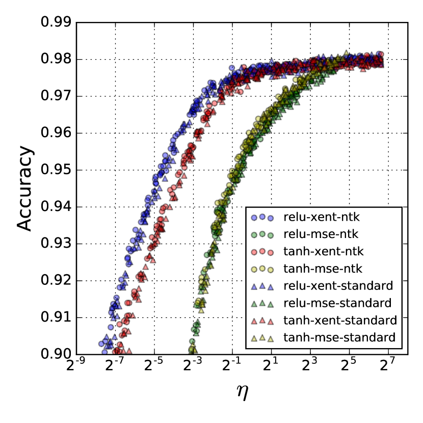
We can verify this property of networks with the standard parameterization experimentally. In Figure S7, we see that for different choices of dataset, activation function and loss function, final performance of two different parameterization leads to similar quality model for similar value of normalized learning rate . Also, in Figure S8, we observe that our results is not due to the parameterization choice and holds for wide networks using the standard parameterization.
Appendix G Convergence of neural network to its linearization, and stability of NTK under gradient descent
In this section, we show that how to use the NTK to provide a simple proof of the global convergence of a neural network under (full-batch) gradient descent and the stability of NTK under gradient descent.
We present the proof for standard parameterization. With some minor changes, the proof can also apply to the NTK parameterization. To lighten the notation, we only consider the asymptotic bound here.
The neural networks are parameterized as in Equation S36.
We make the following assumptions:
Assumptions [1-4]:
-
1.
The widths of the hidden layers are identical, i.e. (our proof extends naturally to the setting as .)
-
2.
The analytic NTK (defined in Equation S42) is full-rank, i.e. We set .
-
3.
The training set is contained in some compact set and for all .
-
4.
The activation function satisfies
(S38)
Assumption 2 indeed holds when and grows non-polynomially for large [13]. Throughout this section, we use to denote some constant whose value may depend on , and and may change from line to line, but is always independent of .
Let denote the parameters at time step . We use the following short-hand
| (S39) | ||||
| (S40) | ||||
| (S41) |
where is the cardinality of the training set and is the output dimension of the network. The empirical and analytic NTK of the standard parameterization is defined as
| (S42) |
Note that the convergence of the empirical NTK in probability is proved rigorously in [37]. We consider the MSE loss
| (S43) |
Since converges in distribution to a mean zero Guassian with covariance , one can show that for arbitrarily small , there are constants and (both may depend on , and ) such that for every , with probability at least over random initialization,
| (S44) |
The gradient descent update with learning rate is
| (S45) |
and the gradient flow equation is
| (S46) |
We prove convergence of neural network training and the stability of NTK for both discrete gradient descent and gradient flow. Both proofs rely on the local lipschitzness of the Jacobian .
Lemma 1 (Local Lipschitzness of the Jacobian).
There is a such that for every , with high probability over random initialization (w.h.p.o.r.i.) the following holds
| (S47) |
where
| (S48) |
The following are the main results of this section.
Theorem G.1 (Gradient descent).
Assume Assumptions [1-4]. For and , there exist , and , such that for every , the following holds with probability at least over random initialization when applying gradient descent with learning rate ,
| (S49) |
and
| (S50) |
Theorem G.2 (Gradient Flow).
Assume Assumptions[1-4]. For , there exist , and , such that for every , the following holds with probability at least over random initialization when applying gradient flow with “learning rate"
| (S51) |
and
| (S52) |
See the following two subsections for the proof.
Remark 1.
G.1 Proof of Theorem G.1
As discussed above, there exist and such that for every , with probability at least over random initialization,
| (S53) |
Let in Lemma 1. We first prove Equation S49 by induction. Choose such that for every Equation S47 and Equation S53 hold with probability at least over random initialization. The case is obvious and we assume Equation S49 holds for . Then by induction and the second estimate of Equation S47
| (S54) |
which gives the first estimate of Equation S49 for and which also implies for . To prove the second one, we apply the mean value theorem and the formula for gradient decent update at step
| (S55) | ||||
| (S56) | ||||
| (S57) | ||||
| (S58) | ||||
| (S59) |
where is some linear interpolation between and . It remains to show with probability at least ,
| (S60) |
This can be verified by Lemma 1. Because [37] in probability, one can find such that the event
| (S61) |
has probability at least for every . The assumption implies
| (S62) |
Thus
| (S63) | ||||
| (S64) | ||||
| (S65) | ||||
| (S66) |
with probability as least if
| (S67) |
Therefore, we only need to set
| (S68) |
To verify Equation S50, notice that
| (S69) | ||||
| (S70) | ||||
| (S71) | ||||
| (S72) |
where we have applied the second estimate of Equation S49 and Equation S47.
G.2 Proof of Theorem G.2
The first step is the same. There exist and such that for every , with probability at least over random initialization,
| (S73) |
Let in Lemma 1. Using the same arguments as in Section G.1, one can show that there exists such that for all , with probability at least
| (S74) |
Let
| (S75) |
We claim . If not, then for all , and
| (S76) |
Thus
| (S77) |
and
| (S78) |
Note that
| (S79) |
which implies, for all
| (S80) |
This contradicts to the definition of and thus . Note that Equation S78 is the same as the first equation of Equation S51.
G.3 Proof of Lemma 1
The proof relies on upper bounds of operator norms of random Gaussian matrices.
Theorem G.3 (Corollary 5.35 [48]).
Let be an random matrix whose entries are independent standard normal random variables. Then for every , with probability at least one has
| (S81) |
For , let
| (S82) | |||
| (S83) |
Let and be any two points in . By the above theorem and the triangle inequality, w.h.p. over random initialization,
| (S84) |
Using this and the assumption on Equation S38, it is not difficult to show that there is a constant , depending on and such that with high probability over random initialization121212These two estimates can be obtained via induction. To prove bounds relating to and , one starts with and , respectively.
| (S85) | ||||
| (S86) |
Lemma 1 follows from these two estimates. Indeed, with high probability over random initialization
| (S87) | ||||
| (S88) | ||||
| (S89) | ||||
| (S90) | ||||
| (S91) | ||||
| (S92) |
and similarly
| (S93) | ||||
| (S94) | ||||
| (S95) | ||||
| (S96) |
G.4 Remarks on NTK parameterization
Theorem G.4 (NTK parameterization).
Assume Assumptions [1-4]. For and , there exist , and , such that for every , the following holds with probability at least over random initialization when applying gradient descent with learning rate ,
| (S97) |
and
| (S98) |
Lemma 2 (NTK parameterization: Local Lipschitzness of the Jacobian).
There is a such that for every , with high probability over random initialization the following holds
| (S99) |
Appendix H Bounding the discrepancy between the original and the linearized network: MSE loss
We provide the proof for the gradient flow case. The proof for gradient descent can be obtained similarly. To simplify the notation, let and . The theorem and proof apply to both standard and NTK parameterization. We use the notation to hide the dependence on uninteresting constants.
Theorem H.1.
Same as in Theorem G.2. For every with , for arbitrarily small, there exist and such that for every , with probability at least over random initialization,
| (S100) |
Proof.
| (S101) | ||||
| (S102) | ||||
| (S103) |
Integrating both sides and using the fact ,
| (S104) | ||||
| (S105) |
Let be the smallest eigenvalue of (with high probability ). Taking the norm gives
| (S106) | ||||
| (S107) | ||||
| (S108) | ||||
| (S109) |
Let
| (S110) | ||||
| (S111) | ||||
| (S112) |
The above can be written as
| (S113) |
Note that is non-decreasing. Applying an integral form of the Grönwall’s inequality (see Theorem 1 in [38]) gives
| (S114) |
Note that
| (S115) |
Then
| (S116) | ||||
| (S117) |
Let . Then
| (S118) |
As it is proved in Theorem G.1, for every , with probability at least over random initialization,
| (S119) |
when . Thus for large and any polynomial (we use here)
| (S120) |
Therefore
| (S121) |
as .
Now we control the discrepancy on a test point . Let be its true label. Similarly,
| (S122) |
Integrating over and taking the norm imply
| (S123) | ||||
| (S124) | ||||
| (S125) | ||||
| (S126) |
Similarly, Lemma 1 implies
| (S127) |
This gives
| (S128) |
Using Equation S118 and Equation S119,
| (S129) |
∎
Appendix I Convergence of empirical kernel
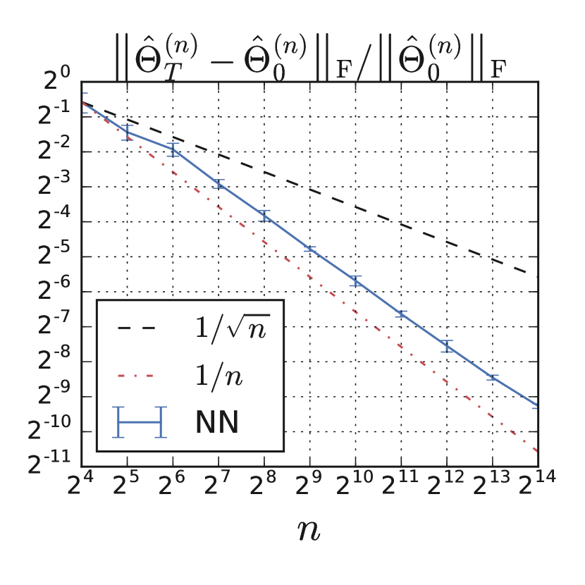
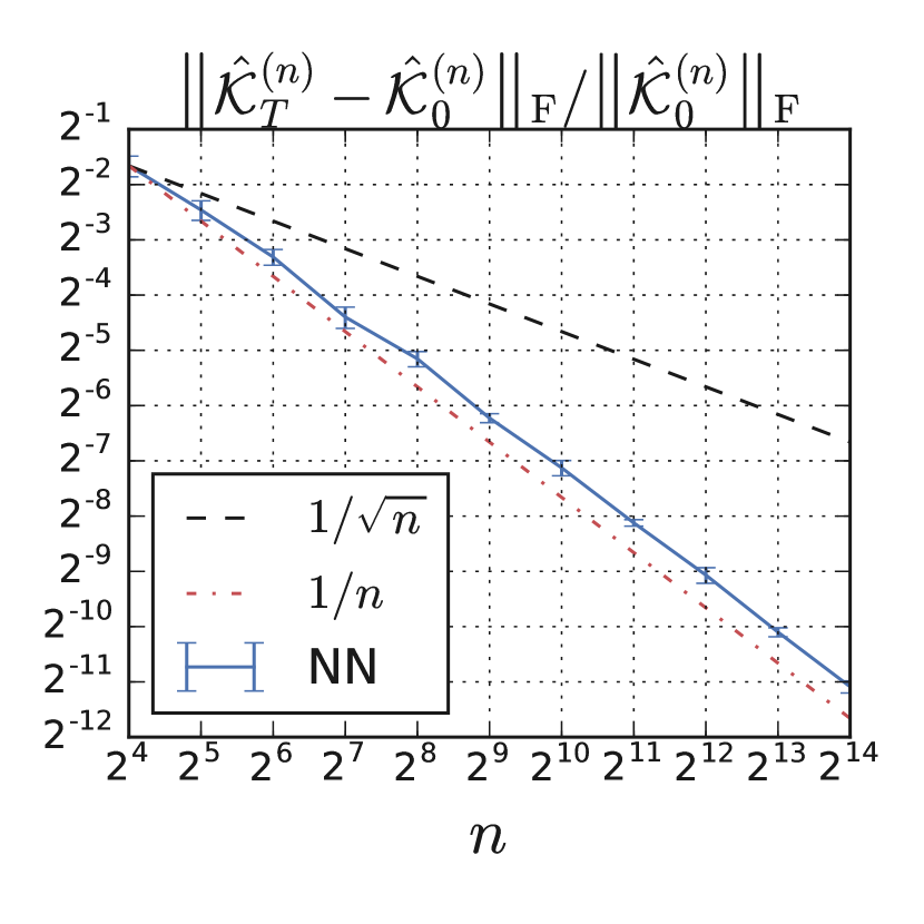
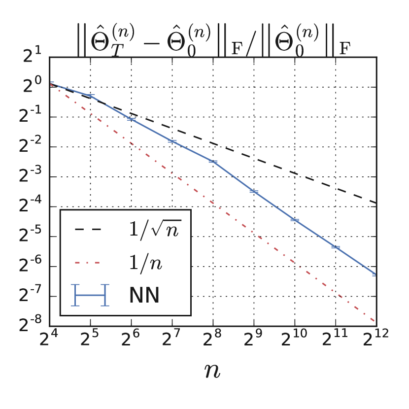
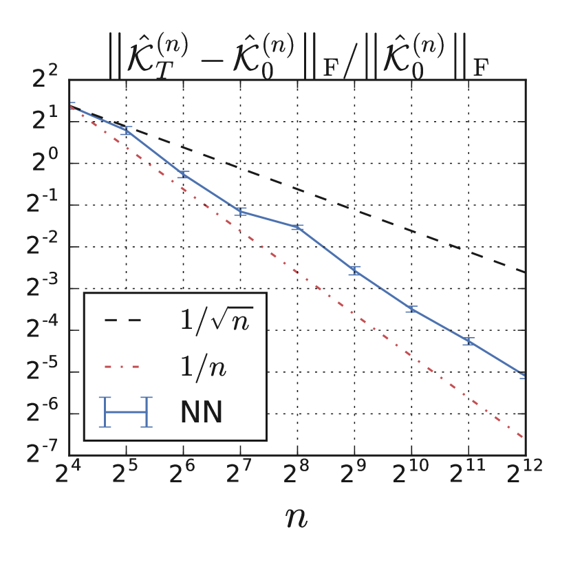
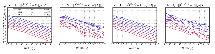
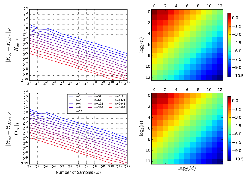
As in Novak et al. [7], we can use Monte Carlo estimates of the tangent kernel (Equation 4) to probe convergence to the infinite width kernel (analytically computed using Equations S26, S29). For simplicity, we consider random inputs drawn from with . In Figure S9, we observe convergence as both width increases and the number of Monte Carlo samples increases. For both NNGP and tangent kernels we observe and , as predicted by a CLT in Daniely et al. [16].
Appendix J Details on Wide Residual Network
| group name | output size | block type |
|---|---|---|
| conv1 | 32 32 | [33, channel size] |
| conv2 | 32 32 | N |
| conv3 | 16 16 | N |
| conv4 | 8 8 | N |
| avg-pool | 1 1 | [8 8] |