SYNTHETIC SPECTRA OF PAIR–INSTABILITY SUPERNOVAE IN 3D

Abstract

Pair–Instability Supernovae (PISNe) may signal the deaths of extremely massive stars in the local Universe or massive primordial stars after the end of the Cosmic Dark Ages. Hydrodynamic simulations of these explosions, performed in 1D, 2D, and 3D geometry, have revealed the strong dependence of mixing in the PISN ejecta on dimensionality. This chemical rearrangement is mainly driven by Rayleigh-–Taylor instabilities that start to grow shortly after the collapse of the carbon–oxygen core. We investigate the effects of such mixing on the spectroscopic evolution of PISNe by post–processing explosion profiles with the radiation diffusion–equilibrium code SNEC and the implicit Monte Carlo – discrete diffusion Monte Carlo (IMC–DDMC) radiation transport code SuperNu. The first 3D radiation transport calculation of a PISN explosion is presented yielding viewing angle–dependent synthetic spectra and lightcurves. We find that while 2D and 3D mixing does not significantly affect the lightcurves of PISNe, their spectroscopic and color evolution is impacted. Strong features of intermediate mass elements dominated by silicon, magnesium and oxygen appear at different phases and reach different intensities depending on the extent of mixing in the silicon/oxygen interface of the PISN ejecta. On the other hand, we do not find a significant dependence of PISN lightcurves and spectra on viewing angle. Our results showcase the capabilities of SuperNu to handle 3D radiation transport and highlight the importance of modeling time–series of spectra in identifying PISNe with future missions.

1 Introduction

Pair–Instability Supernovae (PISNe; Barkat et al. 1967; Rakavy & Shaviv 1967; Ober et al. 1983) are thought to mark the catastrophic explosions of very massive stars that form carbon–oxygen (CO) cores with masses $M_{\rm CO}>$ 60 $M_{\odot}$. The collapse of these massive CO cores is triggered by a softening of the equation of state (EoS) where the adiabatic index, $\gamma_{\rm ad}$, falls below 4/3 due to rapid electron–positron (e^-–e⁺) pair production. As a result, a large amount of carbon and oxygen fuel is ignited leading to the production of large sums ($>$ 1 $M_{\odot}$) of radioactive ⁵⁶Ni. The decay of ⁵⁶Ni can subsequently heat the expanding supernova (SN) ejecta and may even lead to superluminous lightcurves (LCs) with peak luminosities $L_{\rm max}>10^{44}$ erg s^-1 (Heger & Woosley, 2002; Kasen et al., 2011).

The extreme luminosities that can be reached in PISNe suggest that these explosions may be related to some events in the superluminous supernova (SLSN) class (Gal-Yam, 2012, 2018; Moriya et al., 2018). For instance, the hydrogen–poor (SLSN–I) SN 2007bi (Gal-Yam et al., 2009) and the slowly–evolving Type II SN OGLE14–073 (Kozyreva et al., 2018) are often discussed as PISN candidates (see also Inserra et al. 2017; Jerkstrand et al. 2017). All SLSNe observed to date, however, are found at host environments with metallicities $Z>$ 0.1 $Z_{\odot}$ (Neill et al., 2011; Lunnan et al., 2014) suggesting a very large zero–age main–sequence (ZAMS) mass is needed ($M_{\rm ZAMS}\gtrapprox$ 250–300 $M_{\odot}$) to overcome the effects of radiatively–driven mass–loss and to form CO cores that are massive enough to be susceptible to the pair instability (Langer et al., 2007).

In addition, synthetic spectra of PISNe have difficulty in matching the observed spectra of SLSNe at contemporaneous epochs (Dessart et al., 2013; Chatzopoulos et al., 2015; Moriya et al., 2019). Some proposed ways to help mitigate these issues include enhanced mixing due to rapid progenitor rotation allowing PISNe to be encountered at a considerably lower $M_{\rm ZAMS}$ (Chatzopoulos & Wheeler, 2012; Yoon et al., 2012) and large–scale outward mixing of ⁵⁶Ni (Kozyreva & Blinnikov, 2015) (see also Kozyreva et al. 2014a, b). A softer version of PISN that does not lead to the complete disruption of the progenitor star is the pulsational pair–instability supernova mechanism (PPISN; Woosley et al. 2007), encountered for a narrow range of $M_{\rm ZAMS}$ below the limit for full–fledged PISN. PPISN can result in the ejection of multiple shells that can interact with each other yielding several transient events from the same progenitor and, occasionally, to very bright LCs akin to those of SLSNe (Woosley, 2017). These theoretical implications, coupled with observations of massive stars up to $\sim$ 300 $M_{\odot}$ within the young star clusters NGC3603 and R136 in the Milky Way galaxy (Crowther et al., 2010), encourage the notion that while PISNe and PPISNe events must be very rare in the contemporary Universe, they cannot be ruled out.

In addition, very massive ($>$ 200 $M_{\odot}$) metal–poor stars in the early Universe are more likely PISN progenitors (Hirschi, 2007; Joggerst & Whalen, 2011; Pan et al., 2012; Stacy et al., 2012). Population III star formation simulations suggest that the first generation of stars had a top–heavy initial mass function (IMF) (Abel et al., 1998; Bromm et al., 2002; Bromm & Larson, 2004) with a large fraction of them well within the mass limit to encounter PISN (Yoshida et al., 2008; Bromm et al., 2009; Stacy et al., 2012). Given that some PISN models imply very bright lightcurves, these explosions could be detected at large redshifts with upcoming missions such as the James Webb Space Telescope (JWST) and WFIRST (Scannapieco et al., 2005; Hummel et al., 2012; Whalen et al., 2013; Smidt et al., 2015).

The possible link between PISNe, SLSNe and the evolution of very massive stars has driven many efforts to study this mechanism in detail by making use of numerical supercomputer simulations in 2D and 3D (Chen et al., 2014b, a). In particular, the role of mixing induced by Rayleigh-–Taylor (RT) instabilities in 3D and their impact on PISN LCs (Gilmer et al. 2017; hereafter G17), as well as the effects of rapid progenitor rotation on the energetics, dynamics and nucleosynthetic signatures of the explosion have been investigated (Chatzopoulos et al., 2013). As mentioned before, radiation transfer calculations yielding synthetic spectra and LCs for different PISN progenitor properties have also been presented (Dessart et al., 2013; Chatzopoulos et al., 2015; Moriya et al., 2019).

In this work we study the effects of multidimensional mixing on the spectroscopic properties of PISNe by calculating synthetic LCs and spectra for progenitor profiles computed in 1D, 2D and 3D hydrodynamics simulations. To do so, we extract profiles corresponding to regions of high inward and outward mixing of silicon (Si) and nickel (Ni) in the 2D and 3D simulations and post–process them with two different radiation transport codes: SNEC (Morozova et al., 2015), using an equillibrium–diffusion method and SuperNu (Wollaeger et al., 2013) using Implicit Monte Carlo (IMC) and Discrete Diffusion Monte Carlo (DDMC) methods under the assumption of local thermal equillibrium (LTE). We also present the first full 3D PISN synthetic spectra and LCs as a function of viewing angle calculated by SuperNu.

This paper is organized as follows: Section 2 introduces the 1D, 2D and 3D simulations of the PISN model used in this work (P250), Section 3 presents synthetic LCs and spectra for all cases including the first 3D model spectra as a function of viewing angle in the literature and Section 4 summarizes the implications of our results for the PISN mechanism.

2 Multi–Dimensional PISN Models

Multidimensional (2D and 3D) simulations are necessary in order to assess the impact of hydrodynamic instabilities, such as RT, and mixing on the structure and radiative properties of PISNe. The first 2D PISN simulations using the CASTRO (Almgren et al., 2010; Zhang et al., 2011, 2013) code were presented by Joggerst & Whalen (2011) who report little mixing between the O and He layers prior to shock breakout. Chen et al. (2014b, a) also explored the development of hydrodynamic instabilities in both PPISN and PISN in 2D and found that the upper and lower boundaries of the O shell are unstable due to oxygen and helium burning shortly after core bounce. They also explored the role of a reverse shock following SN shock breakout in driving the growth of RT instabilities. Rapidly rotating PISN progenitors simulated in “2.5D” show similar features (Chatzopoulos et al., 2013).

A comprehensive study of mixing in PISN ejecta was presented by G17, who were the first to perform a 3D PISN simulation using the adaptive mesh refinement (AMR) hydrodynamics code FLASH (Fryxell et al., 2000; Dubey et al., 2012). G17 considered a 250 $M_{\odot}$ PISN progenitor model with metallicity 0.07 $Z_{\odot}$ (model P250) and computed with the stellar evolution code GENEC (Ekström et al., 2012; Yusof et al., 2013). Strong radiatively–driven winds lead to complete hydrogen envelope stripping for model P250 so that its pre–PISN mass is $\sim$ 127 $M_{\odot}$ with only $\sim$ 2 $M_{\odot}$ of He retained in the outer layers. The hydrodynamic evolution, explosion and nucleosynthetic burning using 19 isotopes (the Aprox19 network in FLASH; Timmes & Swesty 2000) are then simulated in 1D spherical, 2D cylindrical and 3D cartesian grids.

Model P250 produces an energetic explosion ($\simeq 8.2\times 10^{52}$ erg) synthesizing $\simeq 34$ $M_{\odot}$ of radioactive ⁵⁶Ni. The original 1D and 2D/3D mass–weighted angular–averaged profiles were then post–processed by the radiation–hydrodynamics code STELLA (Blinnikov et al., 1998) yielding a superluminous, slow–evolving bolometric LC (Figure 15 of G17). A comparison of the PISN ejecta composition profiles in the angular–averaged 2D and 3D profiles shown in Figure 8 of G17 suggests stronger mixing in 3D as compared to 2D, especially in the interface between the Si and the O layer. Less extensive mixing is also seen in the Ni/Si interface. This chemical rearrangement is driven by the growth of the RT instability between layers of different composition in the PISN ejecta and is stronger in 3D as expected (Kuchugov et al., 2014).

As mentioned in G17, the RT instabilities were still growing at the end of the simulations. In order to reach the final mass fraction distributions, we needed to extend the evolution with FLASH until mixing has effectively ceased for this work. To accomplish this, we mapped the 1D, 2D, and 3D post–shock data ($r<2.5\times 10^{10}$ cm) from G17 onto larger grids to facilitate expansion of the shock to $r\sim 1\times 10^{11}$ cm. The pre–shock regions of the grid were filled with the densities, temperatures, and mass fractions (effectively uniform) from the GENEC progenitor model. As was done in G17 to extend simulations for input into STELLA, we modify the densities and temperatures to eliminate a jump discontinuity that is caused by the edge density decreasing in the original explosion simulations. However, we choose the radius for this to be $7.56\times 10^{10}$ cm as the fixed radius used in G17 lies outside of our domain of $1\times 10^{11}$ cm.

For the 1D simulation we use the same refinement criteria and bounding resolutions ($1.3\times 10^{8}$ cm and $6.5\times 10^{7}$ cm) from G17. For 2D and 3D we use a nested refinement structure with distinct refinement regions that decrease in refinement outwards. We turn off AMR so that the nested grid structure is static throughout the simulations, as in G17. Due to computational limitations, we could not continue the 3D simulation with the same maximum resolution as in G17 ($3.25\times 10^{7}$ cm). We do, however, map the data exactly from the final FLASH checkpoint files of G17 onto the corresponding interior spatial regions of the larger grids of the extended FLASH simulations. Then, we perform derefinement in the inner refinement regions (a cylinder in 2D and a cube in 3D) so that they merge with their neighboring refinement regions. Thus, evolution of the extended FLASH simulations begin with a maximum refinement of $6.5\times 10^{7}$ cm in their interior refinement regions. Care was taken to ensure that the compositional interfaces never cross the boundaries of the inner refinement regions so that all mixing occurs at maximum resolution. Focusing on the compositional interfaces then, they form in the original simulations from G17 before mixing during their expansion. Then, they suddenly experience a decrease in refinement level and continue to mix and expand during the extended simulation. To understand the effect of the derefinement between simulations, we also computed the 2D simulation without such derefinement. The results of the mixing in the 2D simulation remain practically unchanged, therefore, the mixing in our extended simulations is converged at the resolution used. We halted the simulations when the SN shock wave was very near the edge of the grid ($1\times 10^{11}$ cm). These simulations were performed using XSEDE computing resources (Towns et al., 2014) together with Los Alamos National Lab (LANL) institutional computing resources.

Then, using the data from the final states of the FLASH P250 simulation in 1D, 2D and 3D geometry described in the previous step, we prepared seven profiles for input into the equillibrium–radiation diffusion code SNEC (Morozova et al., 2015) and the IMC–DDMC radiation transport code SuperNu (Wollaeger et al., 2013). These profiles include the direct FLASH output from the 1D P250 simulation (model 1D), and three mass–weighted angular averages each for the 2D and 3D P250 simulation outputs. One such profile is created from the average over all angles (models 2D_AA and 3D_AA), and two profiles from restricting the average over one degree and (one degree)² in the 2D and 3D cases, respectively. The profiles from the restricted averages are meant to represent two opposing viewing angles in which the Si is most effectively mixed outward (models 2D_MO and 3D_MO) or inward (models 2D_MI and 3D_MI) at the Si/O interface. For these restricted averages, all cells whose centroids lay within the range(s) of angles are included.

The averaging proceeded by separating the included cells into radial bins spanning from zero to $1\times 10^{11}$ cm (corresponding to the location of the SN shock wave). For the full mass averages, these bins were uniformly spaced in the 2D cases at $1.5\times 10^{8}$, and in the 3D case at $5\times 10^{8}$. The reason for this was to ensure that enough cells were included in the average for each bin and in 3D there were fewer cells to work with in the stellar envelope (where the simulation resolution was lower than in the 2D simulation). Both bin sizes are more than sufficient for capturing the radial widths of features caused by mixing and were also used for the restricted averages in the region where mixing occurred. However, since even fewer points are available in a restricted average, we needed slightly larger bin sizes for the inner core and envelope regions, both of which have an effectively uniform composition.

After construction of the radial grids the state variables were averaged for each bin (using the individual cell masses for weighting). All of the state variables tracked in the FLASH simulation, save for internal energy and pressure (which can be derived from the density and temperature via the Timmes EoS; Timmes & Swesty 2000), were averaged. Finally, the profiles resulting from the restricted averages were smoothed using a running–line smoother with a span of three (Hastie & Tibshirani, 1990). This was done to eliminate noise due to a relative paucity of points in comparison to the full averages.

Table 1: Basic properties of the PISN (P250) models presented in this work.

Model	$E_{\rm SN}$ (B)	$M_{\rm Ni}$ ($M_{\odot}$)	$\theta^{\dagger}$ (∘)	$\phi^{\dagger}$ (∘)	$L_{\rm max,D}$ ($10^{44}$ erg s-1)	$t_{\rm max,D}$	$L_{\rm max}$ ($10^{44}$ erg s-1)	$t_{\rm max}$	$t_{\rm Si/O}$	$t_{\rm Ni/Si}$
1D	81.9	34.0	–	–	1.06	185.7	1.79	159.5	181.0	216.4
2D_AA	81.9	34.0	–	–	1.06	190.0	1.81	178.7	185.0	220.4
2D_MI	81.9	34.0	18–19	–	1.09	188.7	1.84	176.0	200.7	224.3
2D_MO	81.9	34.0	37–38	–	1.05	182.8	1.78	168.4	169.2	216.4
3D_AA	81.8	33.8	–	–	1.05	185.4	1.74	165.3	181.0	220.4
3D_MI	81.8	33.8	17–18	73–74	0.94	186.9	1.57	171.7	246.0	251.9
3D_MO	81.8	33.8	21–22	69–70	1.00	171.2	1.61	165.9	153.5	202.7
3D_FULL‡	81.8	33.8	–	–	–	–	1.23	185.0	N/A	N/A

Note. — ^† $\theta$ and $\phi$ correspond to the polar and the azimuthal angle, accordingly, in 3D spherical coordinates. For the 2D models, the polar angle $\theta$ is the only coordinate used. The peak luminosity ($L_{\rm peak,D}$) and time of peak luminosity ($t_{\rm peak,D}$) values as computed in SNEC using equilibrium–diffusion radiation transport are also quoted. ^‡ The values quoted for $L_{\rm max}$ and $t_{\rm max}$ in model 3D_FULL correspond to a viewing angle of $\Omega\simeq$ 0^∘ (“edge–on” view). These values vary only by a small amount for different choices of $\Omega$. We do not provide $t_{\rm Si/O}$ and $t_{\rm Ni/Si}$ estimates for the 3D_FULL model because there is not a unique time when the photosphere crosses the Si/O and Ni/Si compositional interfaces in the 3D simulations due to the large extent of the RT mixing. All timescales are expressed in units of days.

Table 1 details the basic properties of the 1D profiles adopted from the 1D, 2D and 3D model P250 simulations for all cases (full angular–average, Si “mixed inwards” and Si “mixed outwards”). Our models include a full 3D profile of model P250 (3D_FULL) that was directly mapped in the 3D homologous grid of SuperNu yielding LCs and spectra as a function of viewing angle (Section 3.3). Table 1 also lists the peak luminosity ($L_{\rm max,D}$ and $L_{\rm max}$ for synthetic LCs computed in SNEC and SuperNu respectively), time to peak luminosity ($t_{\rm max,D}$ and $t_{\rm max}$ for SNEC and SuperNu respectively) and the timescales corresponding to the phase when the SN photosphere crosses the Si/O interface ($t_{\rm Si/O}$) and the Ni/Si interface ($t_{\rm Ni/Si}$) of the ejecta, all measured in units of days.

Figure 1: Density ($\rho$; upper left panel), temperature ($T$; upper right panel), velocity ($v$; lower left panel) and Si mass fraction ($v$; lower right panel) profiles of the 1D PISN model. Black curves correspond to the original FLASH profiles and red curves to the same profiles after mapping to the grid of SNEC. The dashed red curve shows the SNEC profiles after 6 days of homologous hydrodynamic evolution.

Figure 2: Comparisons of density ($\rho$; left panel) and temperature ($T$; right panel) profiles for models: 1D (black curves), 2D_AA, 2D_MI, 2D_MO (red curves) and 2D_AA, 2D_MI, 2D_MO (blue curves) at $t=$ 6 days in the SNEC grid.

Figure 3: Comparison of the abundance profiles at $t=$ 6 days in the SNEC grid. The upper panels correspond to the 1D and the 2D_AA, 2D_MI, 2D_MO models and the lower panels to the 1D and the 3D_AA, 3D_MI, 3D_MO models. In each case, the right panels show a zoom–in to the regions of high Si/O and Ni/Si mixing. The solid curves represent the 1D, the dot–dashed curves the angular–averaged, the dashed curves the Si “mixed–inwards” and the dotted curves the Si “mixed–outwards” models.

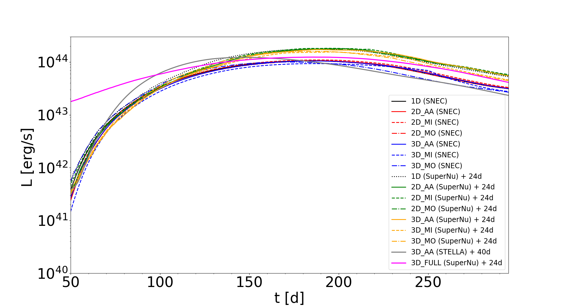
Figure 4: Synthetic bolometric lightcurves from SNEC and SuperNu for the PISN profiles used in this work. The bolometric LC for the angular–averaged 3D P250 model computed with STELLA and presented in (Gilmer et al., 2017) is also shown for comparison.

3 PISN SYNTHETIC LIGHTCURVES AND SPECTRA

3.1 Hydrodynamic Expansion and Radiation Diffusion with SNEC

The seven profiles adopted from the 1D, 2D and 3D P250 model simulations were all at a phase corresponding to SN shock radius of $1\times 10^{11}$ cm and therefore still interior to the stellar envelope of the progenitor star (with radius $\simeq 1.68\times 10^{11}$ cm). In order to compute synthetic spectra with SuperNu, the main objective of this work, we need to provide an input profile that corresponds to a phase shortly after SN shock breakout when the ejecta start to expand homologously. For this reason we decided to follow the post–shock breakout evolution of each of these profiles out to $\sim$ 6 days using the hydrodynamics solver included in the SNEC code. SNEC is a spherically-symmetric Lagrangian radiation-hydrodynamics code designed to follow supernova explosions through the envelope of their progenitor star, produce bolometric (and approximate multi–color) LC predictions, and provide input to spectral synthesis codes for spectral modeling. As such, SNEC also enables us to perform comparisons with P250 LCs computed with SuperNu and STELLA.

Figure 1 shows the density, temperature, velocity and Si mass fraction of the 1D profile at the time of mapping into the Langragian grid of SNEC ($t=$ 0 d) and at $t=$ 6 d when the SN shock reaches a radius of $\sim 10^{15}$ cm. It can be seen that upon mapping to SNEC a monotonically–increasing homologous velocity profile is recovered and the abundance profile of Si (and all other species) remains frozen since nuclear burning has ceased long ago, shorty after the PISN explosion. A comparison of the density and temperature profiles at $t=$ 6 d for all 7 profiles of model P250 discussed here is shown in Figure 2. The abundance profiles for six main species present in the SN ejecta (⁴He, ¹²C12, ¹⁶O, ²⁸Si, ³²S, ⁵⁶Ni) at $t=$ 6 d are shown in Figure 3 including zoomed–in views in regions of high mixing around the Ni/Si and Si/O interfaces. The effect of higher mixing in the 3D_MI and 3D_MO models as compared to their 2D counterparts is clearly seen.

At the beginning of the SNEC simulation, the SN profiles are already in a phase of homologous expansion with high velocities ($\gtrapprox$ 50,000 km s^-1) so we did not have to impose an artificial thermal bomb or a piston explosion to advance the SN evolution. The SNEC calculations include heating by the radioactive decay of ⁵⁶Ni that is the dominant power–input in LCs of PISNe and realistic material opacities adopted from the OPAL (Iglesias & Rogers, 1996) database. The P250 model produces a ⁵⁶Ni yield of $~{}\sim$ 34 $M_{\odot}$ enabling a superluminous bolometric LC ($L_{\rm peak,D}\simeq 1.05\times 10^{44}$ erg s^-1, where “D” stands for “diffusion” implying the radiation diffusion calculation as done in SNEC).

Figure 4 presents the synethic LCs for all models used in this work as computed with SNEC (solid black, red and blue curves), SuperNu (dotted black, green and orange curves) as well as a comparison with the 3D_AA P50 model LC calculated with STELLA (Figure 15 of G17). The peak luminosity agrees within a factor of $\sim$ 2 between the three codes but the timescale to rise to peak luminosity ($t_{\rm max}$) is considerably shorter for the STELLA calculation compared to that found by SNEC and SuperNu (discussed in the next paragraph). This could be due to a variety of reasons including grid resolution, the implementation used to simulate radiation transfer and, more importantly, line opacity values. Investigating these differences is beyond the scope of this paper but we refer to Kozyreva et al. (2017) for a thorough discussion on radiation transfer code–to–code comparison specifically applied to PISN models where the same discrepancy is found between STELLA and the Monte Carlo radiation transport code SEDONA (Kasen et al., 2006). The model LCs exhibit minor differences between the angular–averaged, the Si “mixed–inwards” and the Si “mixed–outwards” cases. The most notable difference is seen for the 3D_MI and 3D_MO models that both reach lower peak luminosities (especially during the post–maximum phase) as compared to all other models. This behavior is consistent between the SNEC and SuperNu results and illustrates the effect of mixing on the total radiated flux from the PISN explosion. This is discussed in more detail in the following paragraph.

3.2 1D Synthetic Spectra with SuperNu

SuperNu is utilized to compute time series of synthetic spectra, synthetic LCs and assess how the radiative properties of PISNe are affected by mixing captured in multidimensional simulations (G17, and this paper). The $t=$ 6 day homologous SNEC profiles for all cases were mapped into the Langragian grid of the IMC–DDMC radiation trasfer code SuperNu (Wollaeger et al., 2013) in 1D spherical geometry. SuperNu simulates time–dependent radiation transport in LTE with matter. It applies the methods of Implicit Monte Carlo (IMC) (Fleck & Cummings, 1971) and Discrete Diffusion Monte Carlo (DDMC) (Densmore et al., 2007) for static or homologously expanding spatial grids. The radiation field affects material temperature but does not affect the motion of the fluid. Multi–group absorption opacity data from hydrogen up to cobalt are included in addition to line data for bound–bound opacities from (Kurucz & Bell, 1995). SuperNu features an improved implementation of opacity regrouping to non–contiguous frequency groups that leads to enhanced performance and computational efficiency (Wollaeger & van Rossum, 2014). This is further enhanced by the capacity of SuperNu to be run on many compute cores in parallel mode. In addition, SuperNu has the capacity to solve the radiative transport and diffusion equations in 1D spherical, 2D cylindrical and 3D spherical, cylindrical or cartesian geometries yielding viewing angle–dependent synthetic LCs and spectra.

The synthetic spectrum of the 1D model at peak luminosity is shown in Figure 5 including comparisons with runs that omitted isotopes for certain atomic species (He, C, O, Mg, Si or S) in order to identify dominant spectral features. It can be seen that the main features are due to intermediate mass elements (IMEs; most prominently Si followed by O, Mg and S), and that the spectrum is very similar to that of regular Type Ia SN events (Cox, 2000). We confirmed this by using the SuperNova IDentification (SNID) code (Blondin & Tonry, 2007) to compare the peak 1D model spectrum to thousands of spectral templates of observed SNe of different types yielding templates of Type Ia SNe as the best matches.

Figure 5: Synthetic SuperNu spectrum at peak luminosity for the 1D model after subtracting contributions from isotopes of He (upper left panel), C (upper right panel), O (middle left panel), Mg (middle right panel), Si (lower left panel) and S (lower right panel). In each panel, the black curve corresponds to the full spectrum and the red curves to the spectrum after subtracting line transition data from all isotopes of the corresponding atom.

Figure 6: Comparisons of synthetic SuperNu spectra for the 1D versus the 2D_AA, 2D_MI, 2D_MO models at different epochs: during peak bolometric luminosity (upper left panel), at the time of peak bolometric luminosity for the 1D model (upper right panel), at 30 d before and 30 d after peak bolometric luminosity (middle panels) and during the transition of the photosphere through regions of high Si/O (lower left panel) and Ni/Si mixing (lower right panel).

Figure 7: Same as Figure 6 but for the 1D versus the 3D_AA, 3D_MI, 3D_MO models.

Figure 8: Color–Color diagrams for the 1D (1D; black circles), 2D (2D_AA, 2D_MI, 2D_MO; green circles, star symbols and squares) and 3D (3D_AA, 3D_MI, 3D_MO orange circles, star symbols and squares) models throughout the PISN evolution. The colors for the 3D_FULL model corresponding to the time of peak luminosity are also shown for comparison (red star symbol).

In particular, the $\lambda$4130 Å, $\lambda$5051 Å and $\lambda$6355 Å Si II features are very strong. The Ca H&K $\lambda\lambda$3934 Å, 3968 Å doublet is identified in the blue part of the spectrum with blends of iron–peak elements populating shorter wavelengths ($\lambda<$ 3500 Å). Other prominent absorption features include the Mg II line at $\lambda$4481 Å and the O I line at $\lambda$7774 Å. Finally, wavelengths in the range 5100 Å $<\lambda<$ 5800 Å are dominated by Fe II and S II line blends. The PISN synthetic spectra obtained in this work are therefore consistent with those calculated for hydrogen–poor PISN progenitors in previous studies indicating spectral evolution that is incompatible with that seen in SLSN–I events at contemporaneous epochs (Dessart et al., 2013; Chatzopoulos et al., 2015; Moriya et al., 2019).

Figures 6 and 7 show comparisons of the 1D model versus the 2D_AA, 2D_MI, 2D_MO and 3D_AA, 3D_MI, 3D_MO sets of models, respectively, at similar epochs. In particular, comparisons are shown for synthetic spectra during peak luminosity ($t=t_{\rm max}$), during peak luminosity as computed in the 1D model ($t=t_{\rm max,1D}=$ 159.5 days), 30 days before and 30 days after peak luminosity and at two phases when the SN photosphere is crossing the Si/O ($t=t_{\rm Si/O}$) and the Ni/Si ($t=t_{\rm Ni/Si}$) interfaces in the PISN ejecta. While the phase corresponding $t_{\rm Si/O}$ is still close to the photospheric phase of the event, the later, $t_{\rm Ni/Si}$ clearly corresponds to the nebular phase of the SN.

The comparison between the 1D and the 2D case indicates that mixing induced by hydrodynamic instabilities shortly after the explosion does have an effect in the intensity and phase of prominent features in PISN spectra, especially during the earlier phase of the event during the rise to peak luminosity. In the earlier phase shown in the middle left panel of Figure 6 ($t=t_{\rm max}-30$ days), the O I $\lambda$7774 Å absorption line appears to be stronger for the 2D_MO model as compared to the other cases. Same holds for the Si II $\lambda$5051 Å feature indicating that outward Si mixing leads to the earlier appearance for these lines as expected since the photosphere is crossing the mixed Si/O interface sooner as compared to the other cases. In contrast, during the $t_{\rm Si/O}$ phase (lower left panel of Figure 6) the opposite behavior is seen: the 2D_MI model Si II $\lambda$6355 Å P Cygni feature is clearly stronger than it is in the other cases for the 2D P250 profiles. During the later, nebular phase ($t_{\rm Ni/Si}$) most spectral features are consistent between the different 2D profiles with the exception of the O I ($\lambda$7774 Å) absorption line that has become weaker for the 2D_MO case by that time.

Figure 9: Synthetic lightcurves (left panel) and spectra at the time of peak luminosity (right panel) as a function of viewing angle from the equatorial plane ($\Omega$) calculated in the 3D SuperNu P250 run (model 3D_FULL).

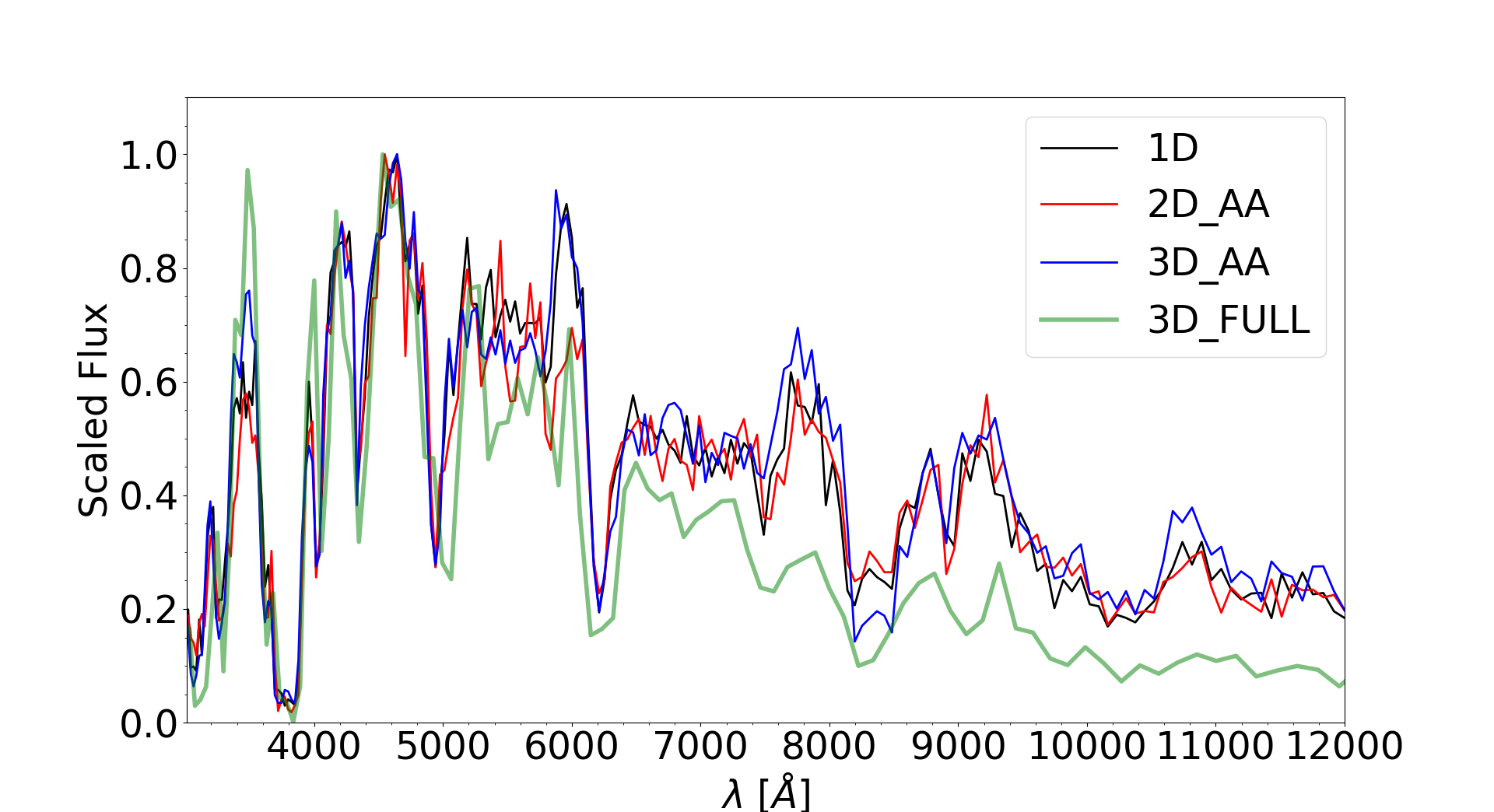
Figure 10: Comparison of the 1D (black curve), 2D_AA (red curve), 3D_AA (blue curve) and 3D_FULL (thick green curve) SuperNu synthetic spectra at time of peak luminosity ($t=t_{\rm max}$).

The effect of mixing is even more pronounced in 3D than it is in 2D (Figure 7). The 3D_MI model possesses a considerably faster spectroscopic evolution than its 3D_AA and 3D_MO counterparts and is characterized by lower intensity spectral features especially at later times ($t>t_{\rm max}+30$ days). As such, during the late phases ($t_{\rm Si/O}$, $t_{\rm Ni/Si}$) the 3D_MI model shows considerable decline in total radiated flux accross the entire spectrum also reflected in the output bolometric luminosity as discussed in Section 3.1 (see also Figure 4). Similarly to the 2D case, the prominent Si and Mg features arise earlier for the 3D_MO so that they appear stronger as compared to the other two 3D cases at the same phase. Finally, during majority of the SN evolution it appears that the pronounced mixing present in both the 3D_MI and 3D_MO makes a difference in the total radiated flux as compared to the angular–averaged case (3D_AA) where the mixing effects are cancelled out. In contrast, the RT mixing in the Ni/Si interface reported by G17 does not appear to have a significant effect in the overall LC or late–time spectra. This is in agreement with the findings of Kozyreva & Blinnikov (2015) who report that extreme – and hard to realize – chemical redistribution in the PISN ejecta is necessary to see a significant impact on the total radiated luminosity.

Perhaps a better way to illustrate the effects of mixing on the evolution of the radiative properties of PISNe is by plotting color–color diagrams for all the models investigated here. Figure 8 shows four color–color diagrams ($B-V$ vs $U-B$, $V-R$ vs $B-V$, $R-I$ vs $V-R$ and $B-R$ vs $B-V$) corresponding to the entire LC evolution of all the models presented in Section 3.2 and to the time of peak luminosity for model 3D_FULL discussed in the next paragraph. To construct these diagrams, we convolved the Johnson/Cousins “standard” filter response curves (Bessell, 1990; Bessell & Murphy, 2012) to the computed spectra in SuperNu. This was done by making use of the Python speclite 0.8 package. The effect of stronger mixing in 3D is apparent in all the color–color diagrams presented in Figure 8. More specifically, 3D models exhibit redder $V-R$ and $R-I$ colors during the rise to peak luminosity. In addition, there seem to be a correlation between the degree of mixing and the resulting color variance during the PISN evolution: larger color scatter is observed for the more heavily mixed 3D, followed by somewhat less scatter for the 2D models and even lesser so for the spherically symmetric 1D models with no mixing. This effect is more discernible in the $V-R$ vs $B-V$ and $R-I$ vs $V-R$ color–color diagrams.

The spectroscopic evolution comparisons for models of different degrees of mixing in the PISN ejecta, as captured by multidimensional simulations of the explosion of a massive H–poor progenitor, clearly illustrates the effects of mixing on the radiative properties of PISNe. Stronger mixing driven by the RT instability shortly after the explosion leads to faster spectroscopic evolution with key spectroscopic features reaching higher intensities while occurring at earlier phases. This unveils the potential to decipher the extent of mixing in PISN ejecta using observed time–series of spectra and potentially study its relation with PISN progenitor structure and explosion energetics.

3.3 3D Synthetic Spectra with SuperNu

While our 1D SuperNu models clearly show the impact of mixing on PISN spectra, they are based on lineout profiles along different directions in the SN ejecta corresponding to varying degrees in the intesity of RT mixing, specifically between the Si and the O interfaces where it appears to be stronger (G17). In order to investigate the total effect of 3D mixing on LCs and spectra as a function of viewing angle we designed and ran the first 3D radiation transport simulation of a PISN in the literature by exploiting the capabilities of SuperNu (model 3D_FULL in Table 1).

To do so, we mapped the FLASH 3D PISN profile used for the 3D_AA model into the grid of SuperNu using a script that coarsens from AMR cells to blocks, which are cells in the 3D Cartesian SuperNu simulation. The PISN ejecta is truncated where the velocity drops sharply, so that it can be approximated as homologous. The homologous relation between radius and velocity is obtained by a linear regression of the radial projection of the velocity. We ensure that the orthogonal component of velocity is small compared to the radial component before simulating with SuperNu.

Figure 9 shows synthetic LCs and spectra at time of peak luminosity as a function of viewing angle with respect to the pole, $\Omega$. It can be seen that the radiative properties of the PISN explosion in 3D are virtually independent of viewing angle. This is not surprising provided that the PISN ejecta structure is not far from spherical symmetry and the effects of large–scale mixing features cancel out. Model 3D_FULL reaches a peak luminosity of $1.3\times 10^{44}$ erg s^-1 that lies in–between the values found in the 1D SuperNu and SNEC models (Section 3.2). Figure 10 presents a comparison of the synthetic spectrum at peak luminosity between the 3D_FULL  (corresponding to the“edge–on” vantage point) and the angular–averaged and spherical models. The same spectroscopic features are noted, albeit at lower flux levels for the 3D_FULL model. This becomes more apparent for the O I feature at $\lambda$7774 Å that appears to be much weaker in the full 3D simulation. Figure 8 also shows the color–color diagrams of the 3D_FULL model corresponding to the time of peak luminosity (red star symbol). Interestingly, the full 3D SuperNu calculation suggests a bluer color evolution for this PISN model as compared to the 1D mixed profiles. This effect may be attributed to the more effective leakage of $\gamma$–rays through regions of lower density due to the clumpy structure of the PISN ejecta caused by the growth of hydrodynamic instabilities, uniquely captured in 3D.

4 Discussion

In this paper we explored the effects of hydrodynamic mixing and progenitor model dimensionality on the radiative properties of PISN explosions by calculating synthetic LCs and time–series of spectra. This was achieved by considering a massive, $M_{\rm ZAMS}=$ 250 $M_{\odot}$ (model P250), progenitor model for which the PISN explosion was simulated in 1D spherical, 2D cylindrical and 3D cartesian geometry as presented in Gilmer et al. (2017). This PISN progenitor was stripped–off its H and He extended envelope prior to reaching the pair–instability regime and thus exploded as a H–poor star with final mass of $\sim$ 127 $M_{\odot}$.

Mixing in the PISN ejecta is triggered mainly due to the growth of the Rayleigh-–Taylor (RT) instability shortly after the collapse of the CO core and it is found to be stronger in 3D than it is in 2D, as expected from Kuchugov et al. (2014). The effects of RT–induced mixing are more pronounced in the Si/O interface while minor effects are also observed in the deeper layers such as the Ni/Si interface. While it has been shown that unphysically strong outward Ni mixing is required in order to significantly affect the peak luminosities and evolution timescales of PISN lightcurves, the effect of mixing on the spectra of these events remained unexplored.

For this reason we post–processed the computed 1D, 2D and 3D model P250 explosion profiles with the radiation diffusion–equillibrium code SNEC and the IMC–DDMC radiation transport code SuperNu focusing on angles of high inward and high outward mixing present in the Si/O interface of the PISN ejecta. Furthermore, we run the first full 3D radiation transport simulation of a PISN model with SuperNu, calculating LCs and synthetic spectra as a function of viewing angle $\Omega$. Model P250 is found to produce a slowly–evolving superluminous SN LCs reaching peak luminosity $>10^{44}$ erg s^-1 and spectra that share a lot of similarities with those of regular Type Ia SNe such as strong features due to intermediate mass elements (Si, S, Mg and O).

Our calculations reveal that hydrodynamic mixing impacts the spectroscopic evolution of PISNe in a several ways. First, the spectroscopic evolution for the models where Si mixing is inwards in the Si/O interface is faster as compared to Si “mixed–outwards” models and this effect is found to be stronger in 3D as compared to the 2D case. Consequently, key spectroscopic features reach higher intensities at earlier phases for the Si “mixed-outwards” models. Comparisons between the mixed and the angular–averaged 3D profiles show that mixing can also lead to different total radiated flux for the mixed models, an effect better exemplified by the color evolution of these models. In contrast, the full 3D radiation transport simulation of the P250 model indicates that the radiative properties of the explosion are not sensitive to viewing angle because large–scale mixing effects are averaged out. This may be different for rapidly rotating PISN progenitors where the overall shape of the expanding SN ejecta becomes highly oblate (Chatzopoulos et al., 2013). In addition, the leakage of $\gamma$–rays through regions of lower density captured in 3D leads to bluer color evolution for the PISN model explored here. This indicates that multi–color photometry of PISN candidates may hold promise in unveiling the identity of these events in the near future. Our 3D radiation transport simulation is the first of its kind and showcases the capabilities of SuperNu to treat explosive outflows with complicated geometries.

The synthetic PISN spectra calculated in this work are in agreement with those presented in previous works and illustrate the difficulty of this mechanism to fit the observations of SLSN–I events given the spectroscopic mismatch at similar epochs. Regardless, the capacity of the PISN model to produce superluminous, slow–evolving transients makes it a relevant candidate for the explosions of rare, extremely massive stars in the local Universe and for massive primordial Population III stars. For the latter, cosmological redshift effects may stretch the duration of the observed LC to several years making it hard to distinguish these early stellar explosions as transient events with upcoming missions such as the JWST and WFIRST suggesting that observations of the color evolution and spectra of these events may be the most suitable way to distinguish them from other sources. Time–dependent, 3D spectroscopic models of these explosions are therefore an important tool to help identify these elusive cosmic catastrophes in the future.

References

- Abel et al. (1998) Abel, T., Anninos, P., Norman, M. L., & Zhang, Y. 1998, ApJ, 508, 518, doi: 10.1086/306410
- Almgren et al. (2010) Almgren, A. S., Beckner, V. E., Bell, J. B., et al. 2010, ApJ, 715, 1221, doi: 10.1088/0004-637X/715/2/1221
- Astropy Collaboration et al. (2018) Astropy Collaboration, Price-Whelan, A. M., Sipőcz, B. M., et al. 2018, AJ, 156, 123, doi: 10.3847/1538-3881/aabc4f
- Barkat et al. (1967) Barkat, Z., Rakavy, G., & Sack, N. 1967, Physical Review Letters, 18, 379, doi: 10.1103/PhysRevLett.18.379
- Bessell & Murphy (2012) Bessell, M., & Murphy, S. 2012, Publications of the Astronomical Society of the Pacific, 124, 140, doi: 10.1086/664083
- Bessell (1990) Bessell, M. S. 1990, Publications of the Astronomical Society of the Pacific, 102, 1181, doi: 10.1086/132749
- Blinnikov et al. (1998) Blinnikov, S. I., Eastman, R., Bartunov, O. S., Popolitov, V. A., & Woosley, S. E. 1998, ApJ, 496, 454, doi: 10.1086/305375
- Blondin & Tonry (2007) Blondin, S., & Tonry, J. L. 2007, ApJ, 666, 1024, doi: 10.1086/520494
- Bromm et al. (2002) Bromm, V., Coppi, P. S., & Larson, R. B. 2002, ApJ, 564, 23, doi: 10.1086/323947
- Bromm & Larson (2004) Bromm, V., & Larson, R. B. 2004, ARA&A, 42, 79, doi: 10.1146/annurev.astro.42.053102.134034
- Bromm et al. (2009) Bromm, V., Yoshida, N., Hernquist, L., & McKee, C. F. 2009, Nature, 459, 49, doi: 10.1038/nature07990
- Chatzopoulos et al. (2015) Chatzopoulos, E., van Rossum, D. R., Craig, W. J., et al. 2015, ApJ, 799, 18, doi: 10.1088/0004-637X/799/1/18
- Chatzopoulos & Wheeler (2012) Chatzopoulos, E., & Wheeler, J. C. 2012, ApJ, 748, 42, doi: 10.1088/0004-637X/748/1/42
- Chatzopoulos et al. (2013) Chatzopoulos, E., Wheeler, J. C., & Couch, S. M. 2013, ApJ, 776, 129, doi: 10.1088/0004-637X/776/2/129
- Chen et al. (2014a) Chen, K.-J., Heger, A., Woosley, S., Almgren, A., & Whalen, D. J. 2014a, ApJ, 792, 44, doi: 10.1088/0004-637X/792/1/44
- Chen et al. (2014b) Chen, K.-J., Woosley, S., Heger, A., Almgren, A., & Whalen, D. J. 2014b, ApJ, 792, 28, doi: 10.1088/0004-637X/792/1/28
- Cox (2000) Cox, A. N. 2000, Allen’s astrophysical quantities
- Crowther et al. (2010) Crowther, P. A., Schnurr, O., Hirschi, R., et al. 2010, MNRAS, 408, 731, doi: 10.1111/j.1365-2966.2010.17167.x
- Densmore et al. (2007) Densmore, J. D., Urbatsch, T. J., Evans, T. M., & Buksas, M. W. 2007, J. Comput. Phys., 222, 485, doi: 10.1016/j.jcp.2006.07.031
- Dessart et al. (2013) Dessart, L., Waldman, R., Livne, E., Hillier, D. J., & Blondin, S. 2013, MNRAS, 428, 3227, doi: 10.1093/mnras/sts269
- Dubey et al. (2012) Dubey, A., Daley, C., ZuHone, J., et al. 2012, ApJS, 201, 27, doi: 10.1088/0067-0049/201/2/27
- Ekström et al. (2012) Ekström, S., Georgy, C., Eggenberger, P., et al. 2012, A&A, 537, A146, doi: 10.1051/0004-6361/201117751
- Fleck & Cummings (1971) Fleck, Jr., J. A., & Cummings, Jr., J. D. 1971, J. Comput. Phys., 8, 313, doi: 10.1016/0021-9991(71)90015-5
- Fryxell et al. (2000) Fryxell, B., Olson, K., Ricker, P., et al. 2000, ApJS, 131, 273, doi: 10.1086/317361
- Gal-Yam (2012) Gal-Yam, A. 2012, Science, 337, 927, doi: 10.1126/science.1203601
- Gal-Yam (2018) —. 2018, arXiv e-prints. https://arxiv.org/abs/1812.01428
- Gal-Yam et al. (2009) Gal-Yam, A., Mazzali, P., Ofek, E. O., et al. 2009, Nature, 462, 624, doi: 10.1038/nature08579
- Gilmer et al. (2017) Gilmer, M. S., Kozyreva, A., Hirschi, R., Fröhlich, C., & Yusof, N. 2017, ApJ, 846, 100, doi: 10.3847/1538-4357/aa8461
- Hastie & Tibshirani (1990) Hastie, T. J., & Tibshirani, R. J. 1990, Generalized additive models (London: Chapman & Hall), 335
- Heger & Woosley (2002) Heger, A., & Woosley, S. E. 2002, ApJ, 567, 532, doi: 10.1086/338487
- Hirschi (2007) Hirschi, R. 2007, A&A, 461, 571, doi: 10.1051/0004-6361:20065356
- Hummel et al. (2012) Hummel, J. A., Pawlik, A. H., Milosavljević, M., & Bromm, V. 2012, ApJ, 755, 72, doi: 10.1088/0004-637X/755/1/72
- Hunter (2007) Hunter, J. D. 2007, Computing In Science & Engineering, 9, 90, doi: 10.1109/MCSE.2007.55
- Iglesias & Rogers (1996) Iglesias, C. A., & Rogers, F. J. 1996, ApJ, 464, 943, doi: 10.1086/177381
- Inserra et al. (2017) Inserra, C., Nicholl, M., Chen, T.-W., et al. 2017, MNRAS, 468, 4642, doi: 10.1093/mnras/stx834
- Jerkstrand et al. (2017) Jerkstrand, A., Smartt, S. J., Inserra, C., et al. 2017, ApJ, 835, 13, doi: 10.3847/1538-4357/835/1/13
- Joggerst & Whalen (2011) Joggerst, C. C., & Whalen, D. J. 2011, ApJ, 728, 129, doi: 10.1088/0004-637X/728/2/129
- Kasen et al. (2006) Kasen, D., Thomas, R. C., & Nugent, P. 2006, ApJ, 651, 366, doi: 10.1086/506190
- Kasen et al. (2011) Kasen, D., Woosley, S. E., & Heger, A. 2011, ApJ, 734, 102, doi: 10.1088/0004-637X/734/2/102
- Kozyreva & Blinnikov (2015) Kozyreva, A., & Blinnikov, S. 2015, MNRAS, 454, 4357, doi: 10.1093/mnras/stv2287
- Kozyreva et al. (2014a) Kozyreva, A., Blinnikov, S., Langer, N., & Yoon, S.-C. 2014a, A&A, 565, A70, doi: 10.1051/0004-6361/201423447
- Kozyreva et al. (2018) Kozyreva, A., Kromer, M., Noebauer, U. M., & Hirschi, R. 2018, MNRAS, 479, 3106, doi: 10.1093/mnras/sty983
- Kozyreva et al. (2014b) Kozyreva, A., Yoon, S.-C., & Langer, N. 2014b, A&A, 566, A146, doi: 10.1051/0004-6361/201423641
- Kozyreva et al. (2017) Kozyreva, A., Gilmer, M., Hirschi, R., et al. 2017, MNRAS, 464, 2854, doi: 10.1093/mnras/stw2562
- Kuchugov et al. (2014) Kuchugov, P. A., Rozanov, V. B., & Zmitrenko, N. V. 2014, Plasma Physics Reports, 40, 451, doi: 10.1134/S1063780X14060038
- Kurucz & Bell (1995) Kurucz, R., & Bell, B. 1995, Atomic Line Data (R.L. Kurucz and B. Bell) Kurucz CD-ROM No. 23. Cambridge, Mass.: Smithsonian Astrophysical Observatory, 1995., 23
- Langer et al. (2007) Langer, N., Norman, C. A., de Koter, A., et al. 2007, A&A, 475, L19, doi: 10.1051/0004-6361:20078482
- Lunnan et al. (2014) Lunnan, R., Chornock, R., Berger, E., et al. 2014, ApJ, 787, 138, doi: 10.1088/0004-637X/787/2/138
- Moriya et al. (2019) Moriya, T. J., Mazzali, P. A., & Tanaka, M. 2019, MNRAS, 259, doi: 10.1093/mnras/stz262
- Moriya et al. (2018) Moriya, T. J., Sorokina, E. I., & Chevalier, R. A. 2018, Space Sci. Rev., 214, 59, doi: 10.1007/s11214-018-0493-6
- Morozova et al. (2015) Morozova, V., Ott, C. D., & Piro, A. L. 2015, SNEC: SuperNova Explosion Code, Astrophysics Source Code Library. http://ascl.net/1505.033
- Neill et al. (2011) Neill, J. D., Sullivan, M., Gal-Yam, A., et al. 2011, ApJ, 727, 15, doi: 10.1088/0004-637X/727/1/15
- Ober et al. (1983) Ober, W. W., El Eid, M. F., & Fricke, K. J. 1983, A&A, 119, 61
- Pan et al. (2012) Pan, T., Kasen, D., & Loeb, A. 2012, MNRAS, 422, 2701, doi: 10.1111/j.1365-2966.2012.20837.x
- Rakavy & Shaviv (1967) Rakavy, G., & Shaviv, G. 1967, ApJ, 148, 803, doi: 10.1086/149204
- Scannapieco et al. (2005) Scannapieco, E., Madau, P., Woosley, S., Heger, A., & Ferrara, A. 2005, ApJ, 633, 1031, doi: 10.1086/444450
- Smidt et al. (2015) Smidt, J., Whalen, D. J., Chatzopoulos, E., et al. 2015, ApJ, 805, 44, doi: 10.1088/0004-637X/805/1/44
- Stacy et al. (2012) Stacy, A., Greif, T. H., & Bromm, V. 2012, MNRAS, 422, 290, doi: 10.1111/j.1365-2966.2012.20605.x
- Timmes & Swesty (2000) Timmes, F. X., & Swesty, F. D. 2000, ApJS, 126, 501, doi: 10.1086/313304
- Towns et al. (2014) Towns, J., Cockerill, T., Dahan, M., et al. 2014, Computing in Science and Engineering, 16, 62, doi: 10.1109/MCSE.2014.80
- Whalen et al. (2013) Whalen, D. J., Even, W., Frey, L. H., et al. 2013, ApJ, 777, 110, doi: 10.1088/0004-637X/777/2/110
- Wollaeger & van Rossum (2014) Wollaeger, R. T., & van Rossum, D. R. 2014, The Astrophysical Journal Supplement Series, 214, 28, doi: 10.1088/0067-0049/214/2/28
- Wollaeger et al. (2013) Wollaeger, R. T., van Rossum, D. R., Graziani, C., et al. 2013, ApJS, 209, 36, doi: 10.1088/0067-0049/209/2/36
- Woosley (2017) Woosley, S. E. 2017, ApJ, 836, 244, doi: 10.3847/1538-4357/836/2/244
- Woosley et al. (2007) Woosley, S. E., Blinnikov, S., & Heger, A. 2007, Nature, 450, 390, doi: 10.1038/nature06333
- Yoon et al. (2012) Yoon, S.-C., Dierks, A., & Langer, N. 2012, A&A, 542, A113, doi: 10.1051/0004-6361/201117769
- Yoshida et al. (2008) Yoshida, N., Omukai, K., & Hernquist, L. 2008, Science, 321, 669, doi: 10.1126/science.1160259
- Yusof et al. (2013) Yusof, N., Hirschi, R., Meynet, G., et al. 2013, MNRAS, 433, 1114, doi: 10.1093/mnras/stt794
- Zhang et al. (2011) Zhang, W., Howell, L., Almgren, A., Burrows, A., & Bell, J. 2011, ApJS, 196, 20, doi: 10.1088/0067-0049/196/2/20
- Zhang et al. (2013) Zhang, W., Howell, L., Almgren, A., et al. 2013, ApJS, 204, 7, doi: 10.1088/0067-0049/204/1/7