Probing the Scale of New Physics
in the $ZZ\gamma$ Coupling at $e^{+}e^{-}$ Colliders

Abstract

The $ZZ\gamma$ triple neutral gauge couplings are absent in the Standard Model (SM) at the tree level. They receive no contributions from dimension-6 effective operators, but can arise from effective operators of dimension-8. We study the scale of new physics associated with such dimension-8 operators that can be probed by measuring the reaction $\,e^{+}e^{-}\!\!\rightarrow\!Z\gamma$ ,  followed by $\,Z\!\!\rightarrow\!\ell\bar{\ell},\nu\bar{\nu}$  decays, at future $e^{+}e^{-}$ colliders including the CEPC, FCC-ee, ILC and CLIC. We demonstrate how angular distributions of the final state mono-photon and leptons can play a key rôle in suppressing SM backgrounds. We further show that using electron/positron beam polarizations can significantly improve the signal sensitivities. We find that the dimension-8 new physics scale can be probed up to the multi-TeV region at such lepton colliders.
KCL-PH-TH/2019-11, CERN-TH/2019-008
e-Print: arXiv:1902.06631.v3

1 . Introduction

At the time of writing, there is no confirmed evidence for phenomena in accelerator experiments that require new physics beyond the Standard Model (SM) John , pending clarifications of the apparent discrepancy between the SM prediction and the experimental value of the anomalous magnetic moment of the muon, and of the apparent anomalies in $b$-hadron decays into strange and charmed particles. It is therefore plausible to assume that the SM particles have the same dimension-4 interactions as in the SM, and seek to characterize possible deviations from SM predictions in terms of higher-dimensional effective operators constructed out of SM fields, whose contributions are suppressed by some power of an underlying new physics scale $\Lambda\gg 100$ GeV dim6 .

This Standard Model Effective Field Theory (SMEFT) approach has mainly been applied with the assumption that only dimension-6 SMEFT operators dim6x contribute to the experimental observables under study reviews . With this restriction, global SMEFT analyses SMEFT have been made of the available data from the LHC and other accelerators, and the sensitivities of experiments at possible future accelerators to the scales of new physics in dimension-6 operators have also been estimated SMEFT ; CLIC-dim6 ; eepp . However, there are some instances in which dimension-6 contributions are absent, and the first SMEFT operators to which experimental measurements are sensitive are those of higher dimensions above6 . For instance, the neutral triple gauge couplings (nTGCs) $ZZ\gamma$ and $Z\gamma\gamma$ provide a promising way of probing directly the relevant dimension-8 operators nTGC1 ; Degrande:2013kka .

These neutral triple gauge couplings are absent in the SM and receive no dimension-6 contributions dim6 ; dim6x . Within the SMEFT approach, the first contributions arise from effective operators of dimension 8 .  These operators involve the Higgs doublet $H$ Degrande:2013kka and the induced nTGCs vanish as the vacuum expectation value $\left<H\right>\!\rightarrow 0$ .  Hence, the origin of these dimension-8 operators is linked to spontaneous electroweak symmetry breaking. This means that probing these neutral TGCs also opens up a new window to the physics of the Higgs boson and electroweak symmetry breaking. We study here how these dimension-8 operators can be probed via the reaction $\,e^{+}e^{-}\!\!\rightarrow\!Z\gamma$  (with $Z\!\rightarrow\ell^{+}\ell^{-}\!,\nu\bar{\nu}$  decays) at future $e^{+}e^{-}$ colliders including CEPC CEPC , FCC-ee FCCee , ILC ILC , and CLIC CLIC , offering one of the rare direct windows on new physics at dimension-8. The test of nTGCs at the FCC-hh via future $pp$(100TeV) collisions was also considered recently pp-nTGC . Other examples where dimension-8 operators dominate include light-by-light scattering gaga-gaga , $\gamma\gamma\rightarrow\gamma\gamma$, which has recently been measured for the first time in heavy-ion collisions at the LHC Aaboud:2017bwk , and $gg\!\rightarrow\!\gamma\gamma$ scattering gg-gaga , which is constrained by ATLAS measurements of events with isolated diphotons in $pp$ collisions at the LHC Aaboud:2017yyg . The effect of dimension-8 operators on Higgs observables was discussed in Sanz8 .

Our analysis framework is described in Section 2. We first discuss in Section 2.1 how the neutral triple-gauge couplings ${ZV\gamma}$ ($V=Z,\gamma$) can be generated by effective dimension-8 operators, and then present cross sections for $\,e^{+}e^{-}\!\!\rightarrow\!Z\gamma$  production in the different $Z$ polarization states $Z_{T,L}$ in Section 2.2. Since the SM produces $Z_{T}\gamma$ final states copiously, with the vector bosons emerging preferentially in the forward and backward directions, we can make use of angular distributions in the $e^{+}e^{-}$ centre-of-mass frame and $Z$ decay frame to separate the SM contribution to $Z\gamma$ final states and distinguish $Z_{L}$ from $Z_{T}$ via their decays into dileptons $\ell^{+}\ell^{-}$.  We study angular observables in Section 3, where the angular distributions are presented in Section 3.1 and their uses for isolating and analyzing new physics contributions are discussed in Section 3.2, with the focus on ${\cal O}(\Lambda^{-4})$ contributions in Section 3.2.1 and on ${\cal O}(\Lambda^{-8})$ contributions in Section 3.2.2. A systematical analysis of the sensitivities to $\Lambda$ by measurements at different $e^{+}e^{-}$ collider energies $\sqrt{s\,}$  from 250 GeV to 5 TeV is presented in Section 3.2.3. We present a refined analysis in Section 3.3 by including additional non-resonant SM backgrounds. In Section 4, we analyze the probe of new physics scale via the invisible decay channel $\,Z\!\rightarrow\nu\bar{\nu}$,  which we then combine with the sensitivity of the dilepton channels $\,Z\!\!\rightarrow\!\ell^{+}\ell^{-}$.  Furthermore, we study the improved sensitivity in Section 5 obtainable by using the $e^{\mp}$ beam polarizations. Finally, we summarize our conclusions in Section 6. The $5\sigma$ sensitivity to $\Lambda$ may reach into the multi-TeV range, depending on the $e^{+}e^{-}$ collision energy, even after taking into account the fact that in many new physics scenarios the SMEFT approach may be valid only when $\Lambda\!\gtrsim\!\!\sqrt{s\,}$ or $\Lambda\!\gtrsim\!\!\sqrt{s}/2$ .  Hence, the reaction $e^{+}e^{-}\!\!\rightarrow\!Z\gamma$  will provide a unique and interesting probe of new physics in $e^{+}e^{-}$ collisions.

2 . Neutral Triple-Gauge Couplings and ${e^{+}e^{-}\!\!\rightarrow\!Z\gamma}$ Production

In this Section, we first discuss the neutral triple-gauge couplings ${ZV\gamma}$ ($V\!=Z,\gamma$), and the corresponding dimension-8 effective operators as their unique lowest-order gauge-invariant formulations in the SMEFT. We then analyze the scattering amplitudes for $e^{+}e^{-}\!\!\rightarrow\!Z\gamma$ ,  considering separately the transverse and longitudinal polarizations of the final-state $Z$ bosons.

2.1 . ${ZV\gamma}$ Coupling from Dimension-8 Operator

The neutral triple gauge couplings (nTGCs) ${ZV\gamma}$ ($V\!=Z,\gamma$) vanish at tree level in the SM and do not receive contributions from any dimension-6 effective operators. However, at the dimension-8 level there are four CP-conserving effective operators that include Higgs doublets and can contribute to the nTGCs,

$$\Delta\mathcal{L}(\text{dim-8})\,=\,\sum_{j=1}^{4}\frac{c_{j}}{\,\tilde{\Lambda}^{4}\,}\mathcal{O}_{j}\,=\,\sum_{j=1}^{4}\frac{\,\text{sign}(c_{j})\,}{\,\Lambda_{j}^{4}\,}\mathcal{O}_{j}\,,$$ (1)

where the dimensionless coefficients $\,c_{j}$ may be ${\cal O}(1)$, with signs $\,\text{sign}(c_{j})=\pm$, and the corresponding ultraviolet (UV) cutoff scales are $\,\Lambda_{j}\equiv\tilde{\Lambda}/|c_{j}|^{1/4}\,$.  The four dimension-8 CP-even effective operators $\mathcal{O}_{j}$ contributing to the nTGCs may be written as Degrande:2013kka ,

$$\mathcal{O}_{\widetilde{B}W} = \mathrm{i}\,H^{\dagger}\widetilde{B}_{\mu\nu}W^{\mu\rho}\!\left\{D_{\!\rho},D^{\nu}\right\}\!H+\text{h.c.},$$ (2a)

$$\mathcal{O}_{B\widetilde{W}} = \mathrm{i}\,H^{\dagger}B_{\mu\nu}\widetilde{W}^{\mu\rho}\!\left\{D_{\!\!\rho},D^{\nu}\right\}\!H+\text{h.c.},$$ (2b)

$$\mathcal{O}_{\widetilde{W}W} = \mathrm{i}\,H^{\dagger}\widetilde{W}_{\mu\nu}W^{\mu\rho}\!\left\{D_{\!\!\rho},D^{\nu}\right\}\!H+\text{h.c.},$$ (2c)

$$\mathcal{O}_{\widetilde{B}B} = \mathrm{i}\,H^{\dagger}\widetilde{B}_{\mu\nu}B^{\mu\rho}\!\left\{D_{\!\!\rho},D^{\nu}\right\}\!H+\text{h.c.},$$ (2d)

where $H$ denotes the SM Higgs doublet. The above operators are Hermitian and we take their coefficients $c_{j}$ to be real for the present study, as we assume CP conservation. We define the dual field strengths $\,\widetilde{B}_{\mu\nu}\!=\epsilon_{\mu\nu\alpha\beta}B^{\alpha\beta}$  and $\,\widetilde{W}_{\mu\nu}\!=\epsilon_{\mu\nu\alpha\beta}W^{\alpha\beta}$,  where $\,W_{\mu\nu}\!=W_{\mu\nu}^{a}\sigma^{a}\!/2\,$ and $\,\sigma^{a}$ denotes Pauli matrices. Among the above operators, one can use the equations of motion (EOM) and integration by parts to show that $\mathcal{O}_{B\widetilde{W}}$ is equivalent to $\mathcal{O}_{\widetilde{B}W}$ up to operators with more currents, or more field-strength tensors, or with quartic gauge boson couplings. Moreover, the operators $\mathcal{O}_{\widetilde{W}W}$ and $\mathcal{O}_{\widetilde{B}B}$ do not contribute to $ZV\gamma$ coupling for on-shell $Z$ and $\gamma$. Thus, there is only one independent CP-conserving dimension-8 operator to be considered in our nTGC study. We choose $\mathcal{O}_{\widetilde{B}W}$ for our analysis, and denote the corresponding cutoff scale $\,\Lambda_{\widetilde{B}W}\!\!=\Lambda\,$, for simplicity.

We note that all the dimension-8 operators in Eq.(2) involve Higgs doublets and the induced nTGCs vanish as the Higgs vacuum expectation value (VEV) $\left<H\right>\!\!\rightarrow\!0$ ,  so their origin is connected to the spontaneous electroweak symmetry breaking (EWSB). Hence, the nTGCs given by dimension-8 operators (2) provide a probe of new physics connected to the spontaneous EWSB. One could write down dimension-8 operators with three gauge-field-strength tensors and two covariant derivatives (but without Higgs doublet) that contribute to the nTGC. For instance, the following pure gauge operator can contribute to nTGC:

$$g\mathcal{O}_{\widetilde{B}WW} = \widetilde{B}_{\!\mu\nu}W^{a\mu\rho}\!\left(D_{\!\!\rho}D_{\lambda}W^{a\nu\lambda}\!+D^{\nu}D^{\lambda}W^{a}_{\!\rho\lambda}\right).$$ (3)

But, the equations of motion (EOM) can be used to convert such operators into operators with two Higgs doublets [cf. Eq.(2)] plus extra operators involving the gauge current of left-handed fermions Degrande:2013kka . In this connection, we note that the EOM of the gauge field $W^{a\mu}$ is given by

$$D^{\nu}W_{\!\mu\nu}^{a}\,=\,\mathrm{i}g\!\left[H^{\dagger}T^{a}D_{\!\mu}H-(D_{\!\mu}H)^{\dagger}T^{a}H\right]+g\,\overline{\psi_{L}}T^{a}\gamma_{\!\mu}\psi_{L}\,,$$ (4)

where $\,T^{a}\!=\tau^{a}/2$  and $\,\psi_{L}\,$ denotes the left-handed weak doublet fermions (leptons or quarks). The summation over the fermion flavor indices is implied in the last term of Eq.(4), Thus, for the pure gauge operator (3), we can make use of the EOM (4) and re-express the new dimension-8 operator (3) as follows:

$$\mathcal{O}_{\!\widetilde{B}WW} \,=\, \mathcal{O}_{\!\widetilde{B}W}\!+\widetilde{B}_{\!\mu\nu}W^{a\mu\rho}\!\left[D_{\!\!\rho}(\overline{\psi_{\!L}}T^{a}\!\gamma^{\nu}\!\psi_{\!L}\!)+D^{\nu}(\overline{\psi_{\!L}}T^{a}\!\gamma_{\!\rho}\psi_{\!L})\right]\!,$$ (5)

where $\mathcal{O}_{\!\widetilde{B}W}$ on the right-hand-side (RHS) is just the original dimension-8 operator (2a). We have explicitly verified that for the reaction $e^{-}e^{+}\!\!\!\rightarrow\!Z\gamma$  with on-shell final states, the contribution from the above dimension-8 pure gauge operator $\,\mathcal{O}_{\!\widetilde{B}WW}$ still vanishes in the limit $\left<H\right>\!\!\rightarrow\!0$ ,  because the extra fermionic contact contribution is proportional to $\,M_{Z}^{2}\propto\!\left<H\right>^{2}$ .  Hence, the key point is that the nTGC, as they are absent in the SM and at the level of dimension-6 operators, can originate from the new physics generating the dimension-8 operators, whose contributions vanish in the limit $\left<H\right>\!\rightarrow\!0$  and thus the existence of these nTGCs hinges upon the spontaneous EWSB. This shows that testing the nTGC via Eq.(2) can provide a new window for probing the new physics connected to the spontaneous EWSB.

We note that the reaction $e^{+}e^{-}\!\!\rightarrow\!Z\gamma$  may also contain possible new physics contribution from a contact vertex $e^{+}e^{-}Z\gamma$ generated by the dimension-8 fermionic operator in Eq.(5). The three types of dimension-8 operators are constrained by Eq.(5), so only two of them are independent. We can choose $\mathcal{O}_{\!\widetilde{B}W}$ and the fermionic contact operator (contributing to $e^{+}e^{-}Z\gamma$) as two independent operators. For the current analysis of testing nTGC at future colliders, we adopt the conventional approach of one operator at a time, as widely used in the literature reviews -gaga-gaga gg-gaga nTGC1 Degrande:2013kka . Hence, we can focus on the dimension-8 operator (2a) for this nTGC study, because Eq.(2a) contributes directly to the nTGC, while the fermionic contact operator does not. Furthermore, we work in the SMEFT formulation for the current study, and follow the common practice in this approach of not considering possible correlations among different dimension-8 operators that may be given by certain specific underlying UV models and are highly model-dependent.

Finally, we can expand Eq.(2a) and derive the following effective $Z\gamma Z^{*}$ coupling from the dimension-8 operator $\mathcal{O}_{\widetilde{B}W}$ in momentum space:

$$\mathrm{i}\,\Gamma^{\mu\nu\alpha}_{Z\gamma Z^{*}}({q}_{1},{q}_{2},{q}_{3}) \,=\, \text{sign}(c_{j})\frac{\,vM_{Z}({q}_{3}^{2}\!-\!M_{Z}^{2})\,}{\,\Lambda^{4}\,}\epsilon^{\mu\nu\alpha\beta}q_{2\beta}\,,$$ (6)

where $\,v/\!\sqrt{2}=\!\left<H\right>\,$ is the Higgs vacuum expectation value. However, $\mathcal{O}_{\widetilde{B}W}$ does not contribute to the $Z\gamma\gamma^{*}$ coupling for on-shell gauge bosons $Z$ and $\gamma$ . Moreover, there is no $\gamma\gamma\gamma^{*}$ triple photon coupling with two photons on-shell. This fact is consistent with our observation that the existence of nTGCs has to rely on the Higgs VEV and thus the spontaneous EWSB, while the residual electromagnetic gauge group $U(1)_{\text{em}}$ holds unbroken.

2.2 . $Z\gamma$ Production at $e^{+}e^{-}$ Colliders

The SM contributes to the production process $e^{-}(p_{1})e^{+}(p_{2})\rightarrow Z(q_{1})\gamma(q_{2})$,  via $t$- and $u$-channel exchange diagrams at tree level. In general, the final-state $Z$ boson may have either longitudinal or transverse polarizations.

Working in the centre of mass (c.m.) frame of the $e^{+}e^{-}$ collider and neglecting the electron mass, we denote the momenta of the initial- and final-state particles as follows:

$$p_{1}=E_{1}(1,0,0,1),~{}~{}~{}~{}p_{2}=E_{1}(1,0,0,-1),$$ (7a)

$$q_{1}=\!\left(E_{Z},\,q\sin\!\theta,\,0,\,q\cos\!\theta\right)\!,~{}~{}~{}~{}q_{2}=q(1,\,-\sin\!\theta,\,0,\,-\cos\!\theta),~{}~{}~{}~{}~{}~{}$$ (7b)

where the electron (positron) energy $\,E_{1}\!=\frac{1}{2}\sqrt{s\,}\,$, the momentum $\,q=\frac{1}{\,2\sqrt{s\,}\,}(s\!-\!M_{Z}^{2})$,  and the $Z$ boson energy $E_{Z}\!=\!\!\sqrt{q^{2}\!+\!M_{Z}^{2}\,}$.  The squared scattering amplitudes for the SM contributions to final states with the different $Z$ polarizations take the following forms:

$$\overline{\left|\mathcal{T}_{\text{sm}}\right|^{2}}[Z_{L}\gamma_{T}] = e^{4}\!\left(8s_{W}^{4}\!-4s_{W}^{2}\!+\!1\right)\!\frac{M_{Z}^{2}\,s}{\,c_{W}^{2}s_{W}^{2}\!\left(s\!-\!M_{Z}^{2}\right)^{2}\,}\,,$$ (8a)

$$\overline{\left|\mathcal{T}_{\text{sm}}\right|^{2}}[Z_{T}\gamma_{T}] = e^{4}\!\left(8s_{W}^{4}\!-4s_{W}^{2}\!+\!1\right)\frac{\left(1\!+\!\cos^{2}\theta\right)\left(s^{2}\!+\!M_{Z}^{4}\right)}{\,2s_{W}^{2}c_{W}^{2}\sin^{2}\theta\left(s\!-\!M_{Z}^{2}\right)^{2}\,}\,,\hskip 22.76219pt$$ (8b)

where we have averaged over the initial-state spins, and used the notations $(s_{W},\,c_{W})=(\sin\!\theta_{W},\,\cos\!\theta_{W})$ with $\theta_{W}\!$ being the weak mixing angle. We have verified that the above formulae agree with the previous results in the literature Degrande:2013kka .

We see from the above equations that the squared amplitude for a final-state longitudinal weak boson $Z_{L}$ is suppressed by $\,1/s\,$ in the high-energy region $\,s\gg M_{Z}^{2}$.  This behaviour can be understood via the equivalence theorem ET , which connects the longitudinal scattering amplitude to the corresponding Goldstone boson amplitude at high energies,

$$\vspace*{-2mm}\mathcal{T}[Z_{L}\gamma_{T}]\,=\,\mathcal{T}[\pi^{0}\gamma_{T}]+O(M_{\!Z}/\!\sqrt{s\,})\,,$$ (9)

where $\pi^{0}$ is the would-be Goldstone boson absorbed by the longitudinally-polarized $Z$ via the Higgs mechanism of the SM. Since the SM does not contain any tree-level $ZV\gamma$ and $\pi^{0}V\gamma$ ($V=Z,\gamma$) triple couplings, at tree level the production processes $e^{+}e^{-}\!\!\rightarrow Z_{L}\gamma_{T}$ and $e^{+}e^{-}\!\!\rightarrow\pi^{0}\gamma_{T}$ must proceed through the $t$-channel electron-exchange process. Since the electron Yukawa coupling $\,y_{e}=\sqrt{2}m_{e}/v=O(10^{-6})\,$ is very small and can be neglected for practical purposes, we have for the SM contributions

$$\mathcal{T}_{\text{sm}}[\pi^{0}\gamma_{T}]\simeq 0\,, \left|\mathcal{T}_{\text{sm}}[Z_{L}\gamma_{T}]\right|^{2}=O(M_{Z}^{2}/s)\,.~{}~{}~{}~{}~{}$$ (10)

This explains the high-energy behavior of Eq.(8a).

We note also that, for the final state with a transverse weak boson $Z_{T}$, Eq.(8b) exhibits a collinear divergence at $\,\theta=0,\pi\,$ due to our neglect of the electron mass $m_{e}\!\simeq 0$ .  In the following analysis we implement a lower cut on the transverse momentum of the final state photon: $\,P_{T}^{\gamma}=q\sin\!\theta>P_{T0}^{\gamma}\,$ to remove the collinear divergence, corresponding to a lower cut on the scattering angle, $\,\sin\theta>\sin\delta=P_{T0}^{\gamma}/q$ .  For $\,\theta\neq 0,\pi$,  Eq.(8b) gives the asymptotic behavior, $\,\mathcal{T}_{\text{sm}}[Z_{T}\gamma_{T}]=O(s^{0})$,  in the high-energy regime $\,s\gg M_{Z}^{2}$ ,  as expected. This completes the explanation why production of the transversely polarized final state $Z_{T}\gamma_{T}$ dominates over that of the longitudinal final state $Z_{L}\gamma_{T}$ .

The contributions of the dimension-8 operator include ${\cal O}(\Lambda^{-4})$ and ${\cal O}(\Lambda^{-8})$ terms. The terms of ${\cal O}(\Lambda^{-4})$ arises from the interference between the dimension-8 operator contribution and the SM contribution, and takes the forms

$$2\Re\texttt{e}\!\left(\overline{\mathcal{T}_{\text{sm}}\mathcal{T}_{(8)}^{*}}\right)[Z_{L}\gamma_{T}] \,=\, \pm\frac{\,e^{2}\!\left(1\!-\!4s_{W}^{2}\right)\,}{\,2s_{W}c_{W}\,}\frac{\,M_{Z}^{2}\,s\,}{\Lambda^{4}}\,,$$ (11a)

$$2\Re\texttt{e}\!\left(\overline{\mathcal{T}_{\text{sm}}\mathcal{T}_{(8)}^{*}}\right)[Z_{T}\gamma_{T}] = \pm\frac{\,e^{2}\!\left(1\!-\!4s_{W}^{2}\right)\,}{\,2s_{W}c_{W}}\frac{\,M_{Z}^{4}\,}{\Lambda^{4}}\,,$$ (11b)

which are consistent with results in the literature Degrande:2013kka . [Here the $\pm$ signs of the ${\cal O}(\Lambda^{\!-4})$ term correspond to the two possible signs of a given dimension-8 operator, $\text{sign}(c_{j})=\pm$,  as shown in Eq.(1).] We see that the contribution to the $Z_{L}\gamma_{T}$ production channel is enhanced relative to that of the $Z_{T}\gamma_{T}$ production channel by a factor of $\,s/M_{Z}^{2}\,$ at ${\cal O}(\Lambda^{-4})$.

The ${\cal O}(\Lambda^{-8})$ terms originate from the pure dimension-8 contributions,

$$\overline{|\mathcal{T}_{(8)}|^{2}}[Z_{L}\gamma_{T}] \,=\, \frac{\,(8s_{W}^{4}\!-\!4s_{W}^{2}\!+\!1)(\cos\!2\theta\!+\!3)\,}{\,32\,}\frac{\,M_{Z}^{2}(s\!-\!M^{2}_{Z})^{2}s\,}{\Lambda^{8}}\,,$$ (12a)

$$\overline{|\mathcal{T}_{(8)}|^{2}}[Z_{T}\gamma_{T}] \,=\, \frac{\,(8s_{W}^{4}\!-\!4s_{W}^{2}\!+\!1)\sin^{2}\!\theta\,}{\,8\,}\frac{\,M_{Z}^{4}(s\!-\!M^{2}_{Z})^{2}\,}{\Lambda^{8}}\,.$$ (12b)

The energy dependence in the above formulas can be directly understood by power counting,

$$\mathcal{T}_{(8)}[Z_{L}\gamma_{T}] \simeq \mathcal{T}_{(8)}[\pi^{0}\gamma_{T}]\sim\frac{\,M_{Z}\,s^{\frac{3}{2}}\,}{\Lambda^{4}}\,,$$ (13a)

$$\mathcal{T}_{(8)}[Z_{T}\gamma_{T}] \sim \frac{\,M_{Z}^{2}\,s\,}{\Lambda^{4}}\,,\,$$ (13b)

which explains the asymptotic high-energy behaviors in Eq.(12) when $s\!\gg\!M_{Z}^{2}$ .  We see that at ${\cal O}(\Lambda^{-8})$ the $Z_{L}\gamma_{T}$ production channel dominates over the $Z_{T}\gamma_{T}$ production channel at high energies $s\gg M_{Z}^{2}$ .

We can understand further the asymptotic behavior of the interference terms (11) for $s\gg M_{Z}^{2}$.  In the case of the final state $Z_{L}\gamma_{T}$, since we have $\,\mathcal{T}_{\text{sm}}[Z_{L}\gamma_{T}]\sim\frac{M_{Z}}{\sqrt{s\,}\,}$  [Eq.(10)] and $\,\mathcal{T}_{(8)}[Z_{L}\gamma_{T}]\sim\frac{\,M_{Z}\,s^{\frac{3}{2}}\,}{\Lambda^{4}}\,$ [Eq. (13a)], we find that their interference term behaves as $\,\overline{\mathcal{T}_{\text{sm}}\mathcal{T}_{(8)}^{*}}[Z_{L}\gamma_{T}]\sim\frac{\,M_{Z}^{2}\,s\,}{\Lambda^{4}}\,$.  This explains nicely the asymptotic behavior of Eq.(11a). However, for the final state $Z_{T}\gamma_{T}$, using the naive power counting from Eqs.(8b) and (13b) we infer the asymptotic behaviors, $\,\mathcal{T}_{\text{sm}}[Z_{T}\gamma_{T}]\sim s^{0}$  and $\,\mathcal{T}_{(8)}[Z_{T}\gamma_{T}]\sim\frac{\,M_{Z}^{2}\,s\,}{\Lambda^{4}}\,$.  Combining these would lead to the following behavior for their interference: $\,\overline{\mathcal{T}_{\text{sm}}\mathcal{T}_{(8)}^{*}}[Z_{T}\gamma_{T}]\sim\frac{\,M_{Z}^{2}\,s\,}{\Lambda^{4}}\,$.  However, this naive power counting contradicts Eq.(11b), where we see that $\,\overline{\mathcal{T}_{\text{sm}}\mathcal{T}_{(8)}^{*}}[Z_{T}\gamma_{T}]\sim\frac{\,M_{Z}^{4}\,s^{0}\,}{\Lambda^{4}}\,$.  Naive power counting fails in this case for a nontrivial reason, which is connected to the special structure of the helicity amplitude $\mathcal{T}_{(8)}[Z_{T}\gamma_{T}]$.  We see from Eqs.(78e) and (79) of Appendix A.1 that the off-diagonal helicity amplitides $\mathcal{T}_{(8)}[Z_{T}\gamma_{T}]$ with $\lambda\lambda^{\prime}=+-,-+$ vanish because of the antisymmetric tensor $\,\epsilon^{\mu\nu\alpha\beta}\,$ contained in the $Z\gamma Z^{*}$ vertex [Eq.(6)]. Hence, the energy dependence of $\,\overline{\mathcal{T}_{\text{sm}}\mathcal{T}_{(8)}^{*}}[Z_{T}\gamma_{T}]$  is determined by the diagonal helicity amplitudes with $\lambda\lambda^{\prime}=++,--$. The SM amplitude $\mathcal{T}_{\text{sm}}[Z_{T}\gamma_{T}]$ has a negative power of energy $\propto s^{-1}$  in its diagonal helicity amplitudes as shown in Eq.(77e). This explains neatly the high-energy behavior $\,\overline{\mathcal{T}_{\text{sm}}\mathcal{T}_{(8)}^{*}}[Z_{T}\gamma_{T}]\sim\frac{\,M_{Z}^{4}\,s^{0}\,}{\Lambda^{4}}\,$,  in agreement with Eq.(11b).

3 . Probing New Physics in the $ZV\gamma$ Coupling at $e^{+}e^{-}$ Colliders

In this section, we first analyze the kinematical structure of the reaction $\,e^{+}e^{-}\!\!\rightarrow Z\gamma\,$ followed by $Z$ decays into pairs of charged leptons $\ell^{\pm}$. We then propose suitable kinematical cuts to suppress effectively the SM backgrounds, and derive the optimal sensitivity reach for the scale of the new physics in the $ZV\gamma$ coupling. In Section 3.1, we analyze the angular observables for $Z\gamma\,$ production with $Z\!\rightarrow\!\ell^{+}\ell^{-}$, and then study probes of the new physics contributions at ${\cal O}(\Lambda^{-4})$ in Section 3.2.1 and at ${\cal O}(\Lambda^{-8})$ in Section 3.2.2, making use of angular observables to suppress the SM backgrounds for the specific $e^{+}e^{-}$ collision energy $\sqrt{s}=3$ TeV. Then, we extend the analysis to other collider energies $\sqrt{s}=(250,\,500,\,1000,\,5000)$ GeV in Section 3.2.3, showing the increase in sensitivity obtainable from increasing the collider energy. Finally, in Section 3.3, we present a more complete background analysis including additional non-resonant SM backgrounds with the same final state $\ell^{-}\ell^{+}\gamma$ (but $\ell^{-}\ell^{+}$ not coming from $Z$ decay).

3.1 . Analysis of Angular Observables

In this subsection, we analyze the kinematical observables for the reaction $\,e^{+}e^{-}\!\!\rightarrow Z\gamma\,$ followed by the leptonic decays $\,Z\!\rightarrow\!\ell^{+}\ell^{-}$.  We illustrate the kinematics in Fig. 1, where the scattering plane is determined by the incident $e^{-}e^{+}$ and the outgoing $\,Z\gamma$  in the collision frame (with scattering angle $\theta$ ), and the directions of the final-state leptons $\ell^{-}\ell^{+}$ determine the decay plane. We denote the angle between the two planes as $\phi$ in the laboratory frame (which is equal to $\phi_{*}$ in the $Z$ rest frame).

In order to study the leptonic final states $\,Z(q_{1})\!\rightarrow\ell^{-}(k_{1})\ell^{+}(k_{2})$,  we denote the lepton momenta as follows in the $Z$ rest frame:

$$k_{1} = \frac{\,M_{Z}\,}{2}\left(1,\,\sin\!\theta_{*}\!\cos\!\phi_{*},\,\sin\!\theta_{*}\!\sin\!\phi_{*},\,\cos\!\theta_{*}\right),$$ (14a)

$$k_{2} = \frac{\,M_{Z}\,}{2}\left(1,\,-\sin\!\theta_{*}\!\cos\!\phi_{*},\,-\sin\!\theta_{*}\!\sin\!\phi_{*},\,-\cos\!\theta_{*}\right).$$ (14b)

Here the positive $z_{*}$ direction in the $Z$ rest frame is chosen to be opposite to the final-state photon direction in the laboratory frame, and $\theta_{*}$ denotes the angle between the positive $z_{*}$ direction and the $\ell^{-}$ direction in the $Z$ rest frame. When boosted back to the $e^{-}e^{+}$ collision frame (laboratory frame), the angle $\theta_{*}$ changes but the azimuthal angle $\phi_{*}$ is invariant. This is why the angle $\phi_{*}$ is equal to the angle $\phi$ between the scattering plane (defined by the incoming $e^{-}e^{+}$ directions and the outgoing $Z\gamma$ directions) and $Z$ decay plane (defined by the outgoing $\ell^{-}$ and $\ell^{+}$ directions) in the $e^{-}e^{+}$ collision frame.

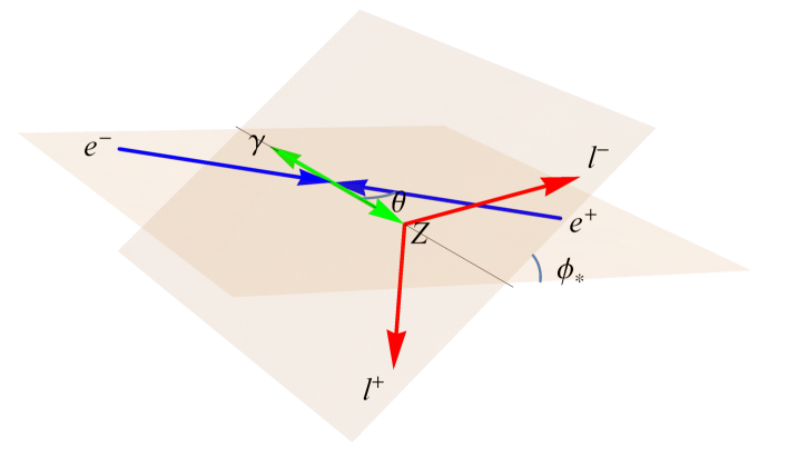
Figure 1: Illustration of the kinematical structure of the reaction $\,e^{+}e^{-}\!\!\rightarrow Z\gamma\,$ followed by the leptonic decay $\,Z\!\rightarrow\ell^{+}\ell^{-}$  in the laboratory frame ($\,e^{-}e^{+}$​ collision frame).

Imposing a lower cut on the scattering angle in the laboratory frame, $\,\sin\theta>\sin\delta\,$ (where $\delta\ll 1$), will correspond to a lower cut on the transverse momentum of the final-state photon $\,P_{T}^{\gamma}>q\sin\delta$ .  With this lower cut, we find the following total cross section for $Z\gamma$ production:

$$\sigma(Z\gamma) \,=\, \frac{\,e^{4}(c_{L}^{2}\!+\!c_{R}^{2})\!\!\left[-(s\!-\!M^{2}_{Z})^{2}\!-\!2(s^{2}\!+\!M_{Z}^{4})\ln\!\left(\sin\!\frac{\delta}{2}\right)\right]\,}{\,8\pi s_{W}^{2}c_{W}^{2}(s\!-\!M^{2}_{Z})s^{2}\,}\hskip 42.67912pt$$

$$\pm\frac{\,e^{2}(c_{L}^{2}\!-\!c_{R}^{2})M_{Z}^{2}\!\left(s\!-\!M_{Z}^{2}\right)\!\!\left(s\!+\!M^{2}_{Z}\right)\,}{\,8\pi s_{W}c_{W}\Lambda^{4}s^{2}\,}$$

$$+\frac{\,(c_{L}^{2}\!+\!c_{R}^{2})M_{Z}^{2}\!\left(s\!+\!M^{2}_{Z}\right)\!\!\left(s\!-\!M^{2}_{Z}\right)^{\!3}\,}{\,48\pi\Lambda^{8}s^{2}\,}+O(\delta)\,,$$

$$\,=\, \frac{\,e^{4}(1\!-\!4s_{W}^{2}\!+\!8s_{W}^{4})\!\!\left[-(s\!-\!M^{2}_{Z})^{2}\!-\!2(s^{2}\!+\!M_{Z}^{4})\ln\!\left(\sin\!\frac{\delta}{2}\right)\right]\,}{\,32\pi s_{W}^{2}c_{W}^{2}(s\!-\!M^{2}_{Z})s^{2}\,}\hskip 42.67912pt$$

$$\pm\frac{\,e^{2}(1\!-\!4s_{W}^{2})M_{Z}^{2}\!\left(s\!-\!M_{Z}^{2}\right)\!\!\left(s\!+\!M^{2}_{Z}\right)\,}{\,32\pi s_{W}c_{W}\Lambda^{4}s^{2}\,}$$

$$+\frac{\,(1\!-\!4s_{W}^{2}\!+\!8s_{W}^{4})M_{Z}^{2}\!\left(s\!+\!M^{2}_{Z}\right)\!\!\left(s\!-\!M^{2}_{Z}\right)^{\!3}\,}{\,192\pi\Lambda^{8}s^{2}\,}+O(\delta)\,,$$

where the $\pm$ signs of the $O(\Lambda^{-4})$ interference term come from $\,\text{sign}(c_{j})\!=\!\pm$  for each given dimension-8 operator, as shown in Eq.(1). In Eq.(15),  $(c_{L},c_{R})=(s_{W}^{2}-\mbox{$\frac{\,{1}\,}{2}$},\,s_{W}^{2})$  denote the $Z$ gauge couplings to the (left, right)-handed electron.

We compute numerically the exact cross sections for $e^{+}e^{-}\!\rightarrow Z\gamma$, as a function of the new physics scale $\Lambda$ and for different collider energies. imposing a photon transverse momentum cut $\,P_{T}^{\gamma}=q\sin\delta$  with $\delta>0.2$ :

$$\sqrt{s\,}\!=250\text{GeV}, \sigma(Z\gamma)=\left[7749\pm 8.90\!\left(\!\frac{\,0.5\text{TeV}\,}{\Lambda}\!\right)^{\!\!4}\!+1.98\!\left(\!\frac{\,0.5\text{TeV}\,}{\Lambda}\!\right)^{\!\!8}\right]\!\text{fb}\,,~{}~{}~{}~{}~{}~{}~{}~{}$$ (16a)

$$\sqrt{s\,}\!=500\text{GeV}, \sigma(Z\gamma)=\left[1624\pm 1.38\!\left(\!\frac{\,0.8\text{TeV}\,}{\Lambda}\!\right)^{\!\!4}\!+0.929\!\left(\!\frac{\,0.8\text{TeV}\,}{\Lambda}\!\right)^{\!\!8}\right]\!\text{fb}\,,$$ (16b)

$$\sqrt{s\,}\!=1\text{TeV}, \sigma(Z\gamma)=\left[390\pm 0.566\!\left(\!\frac{\,\text{TeV}\,}{\Lambda}\!\right)^{\!\!4}+2.62\!\left(\!\frac{\,\text{TeV}\,}{\Lambda}\!\right)^{\!\!8}\right]\!\text{fb}\,,$$ (16c)

$$\sqrt{s\,}\!=3\text{TeV}, \sigma(Z\gamma)=\left[42.9\pm 0.0354\!\left(\!\frac{\,2\text{TeV}\,}{\Lambda}\!\right)^{\!\!4}+0.843\!\left(\!\frac{\,2\text{TeV}\,}{\Lambda}\!\right)^{\!\!8}\right]\!\text{fb}\,,$$ (16d)

$$\sqrt{s\,}\!=5\text{TeV}, \sigma(Z\gamma)=\left[15.4\pm 0.0145\!\left(\!\frac{\,2.5\text{TeV}\,}{\Lambda}\!\right)^{\!\!4}+1.09\!\left(\!\frac{\,2.5\text{TeV}\,}{\Lambda}\!\right)^{\!\!8}\right]\!\text{fb}\,.~{}~{}~{}~{}~{}~{}~{}~{}~{}~{}$$ (16e)

As we show in Section 3.2-3.3 (cf. Table 2), the sensitivity reach of $\,\Lambda$  in each case is such that on the right-hand-side of the corresponding formula above, the ratio inside each $\left[{\cdots}\right]$  is ${\cal O}(1)$. Thus, we see from Eq.(16) that, for the relevant sensitivity reaches of $\Lambda$, the contributions of the dimension-8 operator are always much smaller than the SM contributions, so the perturbation expansion is valid. Also, Eq.(16) shows that for $\sqrt{s\,}<1$ TeV the ${\cal O}(\Lambda^{\!-4})$ contribution is dominant, whereas for $\sqrt{s\,}\gtrsim 1$ TeV, the ${\cal O}(\Lambda^{\!-8})$ contribution becomes dominant. This is because the ${\cal O}(\Lambda^{\!-8})$ contributions have higher energy dependence than the ${\cal O}(\Lambda^{\!-4})$ contributions, as shown in Eqs.(11)-(12).

The total cross section for  $e^{+}e^{-}\!\rightarrow Z\gamma\rightarrow\ell^{+}\ell^{-}\gamma$  is given by the product

$$\sigma(\ell^{+}\ell^{-}\gamma)\,=\,\sigma(Z\gamma)\times\text{Br}(\ell^{+}\ell^{-})\,.$$ (17)

The differential cross section is a function of the three kinematical angles $(\theta,\,\theta_{*},\,\phi_{*})$, and is computed from the helicity amplitudes (A.2)-(A.2) in Appendix-A.2. We define the normalized angular distribution function as

$$f_{\xi}^{j}\,=\,\frac{\mathrm{d}\sigma_{\!j}}{\,\sigma_{\!j}\mathrm{d}\xi\,}\,,$$ (18)

where $\,\xi=\theta,\,\theta_{*},\,\phi_{*}$,  and $\,\sigma_{j}$ (with $j=0,1,2$) represents the SM contribution ($\sigma_{0}$), the ${\cal O}(\Lambda^{-4})$ contribution ($\sigma_{1}$), and the ${\cal O}(\Lambda^{-8})$ contribution ($\sigma_{2}$), respectively.

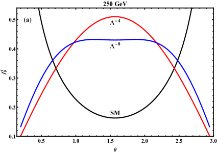
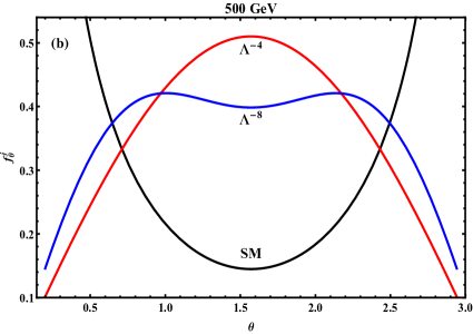
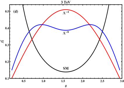
Figure 2: Normalized angular distributions in the polar scattering angle $\theta$ in the laboratory frame for different collision energies, $\sqrt{s}=(250\,\text{GeV},500\,\text{GeV},1\,\text{TeV},3\,\text{TeV})$. In each plot, the black, red and blue curves denote the contributions from the SM, the ${\cal O}(\Lambda^{-4})$ and ${\cal O}(\Lambda^{-8})$ terms, respectively. We use a polar angle cut $\,\delta=0.2\,$ for illustration.

We find the following normalized polar angular distribution functions $\,f_{\theta}^{j}\,$ and $\,f_{\theta_{*}}^{j}$,

$$f_{\theta}^{0} = -\frac{\,\csc\!\theta\!\left[3s^{2}\!+\cos\!2\theta(s\!-\!M_{Z}^{2})^{2}\!+2M_{Z}^{2}s+3M_{Z}^{4}\right]\,}{\,4\!\left[(s\!-\!M_{Z}^{2})^{2}\!+2(s^{2}\!+\!M_{Z}^{4})\!\ln\!\left(\sin\frac{\delta}{2}\right)\right]\,}\,,$$ (19a)

$$f_{\theta}^{1} = \frac{1}{2}\sin\theta\,,$$ (19b)

$$f_{\theta}^{2} = \frac{\,3\sin\!\theta\!\left[3s+\cos\!2\theta(s\!-\!2M_{Z}^{2})+2M_{Z}^{2}\right]\,}{\,16(s+\!M_{Z}^{2})\,}\,;$$ (19c)

and

$$f_{\theta_{*}}^{0} = \frac{\,3\sin\!\theta_{*}(3\!+\!\cos\!2\theta_{*})\,}{16}+\frac{3\sin\!\theta_{*}(1+3\cos\!2\theta_{*})M_{Z}^{2}\,s\,}{\,8\!\left[(s\!-\!M_{Z}^{2})^{2}\!+\!2(s^{2}\!+\!M_{Z}^{4})\ln\!\left(\!\sin\!\frac{\delta}{2}\right)\right]}+O(\delta)\,,\hskip 28.45274pt$$ (20a)

$$f_{\theta_{*}}^{1} = \frac{\,3\sin\!\theta_{*}\!\left[2s\!-\!\cos\!2\theta_{*}(2s\!-\!M_{Z}^{2})\!+\!3M_{Z}^{2}\right]}{16(s+\!M_{Z}^{2})}+O(\delta)\,,$$ (20b)

$$f_{\theta^{*}}^{2} = \frac{\,3\sin\!\theta_{*}\!\left[2s\!-\!\cos\!2\theta_{*}\!(2s\!-\!M_{Z}^{2})\!+\!3M_{Z}^{2}\right]}{16(s+M_{Z}^{2})}+O(\delta)\,.$$ (20c)

Then, we compute the normalized azimuthal angular distribution functions $\,f_{\phi_{*}}^{j}\,$ as follows,

$$f_{\phi_{*}}^{0} = \frac{1}{2\pi}+\frac{3\pi^{2}(c_{L}^{2}\!-\!c_{R}^{2})^{2}M_{Z}\sqrt{s}\,(s\!+\!M_{Z}^{2})\cos\!\phi_{*}\!-8(c_{L}^{2}\!+\!c_{R}^{2})^{2}M_{Z}^{2}\,s\cos\!2\phi_{*}\,}{\,16\pi(c_{L}^{2}\!+\!c_{R}^{2})^{2}\!\left[(s\!-\!M_{Z}^{2})^{2}\!+2(s^{2}\!+\!M_{Z}^{4})\!\ln\!\left(\!\sin\frac{\delta}{2}\right)\right]\,}+O(\delta),\hskip 11.38109pt$$ (21a)

$$f_{\phi_{*}}^{1} = \frac{1}{2\pi}-\frac{\,9\pi^{2}\!\sqrt{s}\,(s\!+\!M_{Z}^{2})\cos\!\phi_{*}\!-\!32M_{Z}\,s\cos\!2\phi_{*}\,}{\,128\pi M_{Z}(s\!+\!M_{Z}^{2})\,}+O(\delta),$$ (21b)

$$f_{\phi_{*}}^{2} = \frac{1}{2\pi}-\frac{\,9\pi(c_{L}^{2}\!-\!c_{R}^{2})^{2}M_{Z}\sqrt{s}\cos\!\phi_{*}\,}{\,128(c_{L}^{2}\!+\!c_{R}^{2})^{2}(s\!+\!M_{Z}^{2})\,}+O(\delta)\,,$$ (21c)

where the coefficients  $(c_{L},\,c_{R})=(s_{W}^{2}\!-\!\mbox{$\frac{\,{1}\,}{2}$},\,s_{W}^{2})$  are the gauge couplings of the $Z$ boson to the (left, right)-handed leptons. Here we have again chosen a lower cutoff $\,\delta\ll 1$  on the polar scattering angle $\theta$,  which corresponds to a lower cut on the transverse momentum of the final state photon, $\,P_{T}^{\gamma}>q\sin\!\delta$.

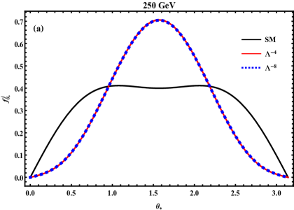
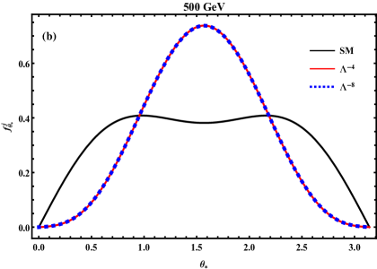
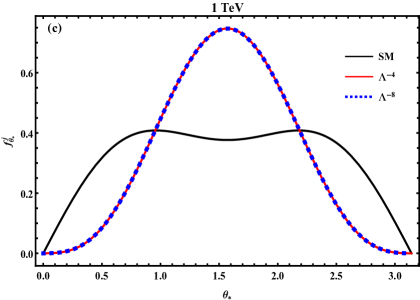
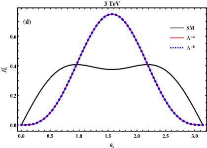
Figure 3: Normalized angular distribution in the polar angle $\theta_{*}$ in the $Z$ decay frame for different collision energies, $\sqrt{s}=(250\,\text{GeV},500\,\text{GeV},1\,\text{TeV},3\,\text{TeV})$. In each plot, the black, red and blue curves denote the contributions from the SM, the ${\cal O}(\Lambda^{-4})$ and ${\cal O}(\Lambda^{-8})$ terms, respectively, where the red and blue curves exactly overlap. We use a laboratory polar angle cut $\delta=0.2$ for illustration.

As a side remark, we note that if the $Z$ boson were a stable particle, one could in principle measure its polarization directly to extract the new physics signal of the dimension-8 operator. However, since the $Z$ decays rapidly into fermion pairs, the contributions of the out-going longitudinal $Z_{L}$ and transverse $Z_{T}$ intermediate states interfere in the angular distributions of the fermions produced in $Z_{L}$ and $Z_{T}$ decays. Such interference effects appear as the $\phi_{*}$ angular dependence in Eq.(21).

Using the above results, we present numerical results for the normalized angular distribution functions of $\,\theta$,  $\theta_{*}$, and $\phi_{*}$,  in Fig. 2, Fig. 3, and Fig. 4, respectively. In each figure, the four plots have input different collision energies $\sqrt{s}=(250\,\text{GeV},500\,\text{GeV},1\,\text{TeV},$ $3\,\text{TeV})$, corresponding to the expected collision energies of the ILC, CEPC and FCC-ee, of possible ILC energy upgrades, and the design energy of CLIC. In each plot, we use black, blue, and red curves to denote the contributions from the SM, the ${\cal O}(\Lambda^{-4})$ term and the ${\cal O}(\Lambda^{-8})$ term, respectively. In this analysis, we set a lower cut $\,\sin\theta>\sin\delta$ (with $\delta=0.2$)  for illustration, which corresponds to a lower cut on the photon transverse momentum $\,P_{T}^{\gamma}>q\sin\delta\simeq 0.2q\,$.

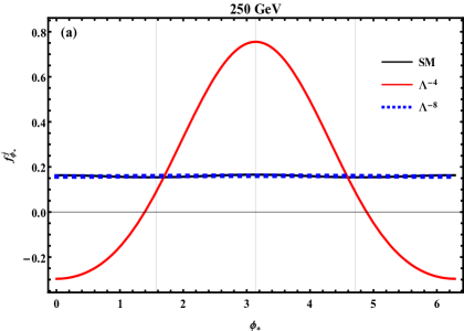
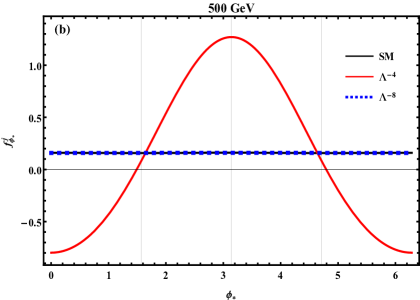
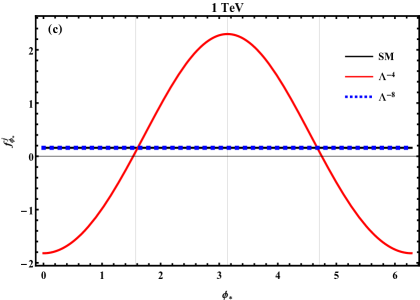
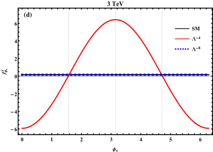
Figure 4: Normalized angular distribution in the azimuthal angle $\phi_{*}$ for different collision energies, $\sqrt{s}=(250\,\text{GeV},500\,\text{GeV},1\,\text{TeV},3\,\text{TeV})$. In each plot, the black, red and blue curves denote the contributions from the SM, the ${\cal O}(\Lambda^{-4})$ and ${\cal O}(\Lambda^{-8})$ terms, respectively, where the blue and black curves nearly overlap. We use a laboratory polar angle cut $\delta=0.2$ for illustration.

It is of interest to examine the behaviours of the angular distribution functions $\,f_{\xi}^{j}$  in the high-energy limit $\,s\gg M_{Z}^{2}$ .  For all the functions $f_{\theta}^{j}$ and $f_{\theta_{*}}^{j}$, the coefficients of all trigonometric functions approach constants. This is why Figs. 2 and 3 show that the distributions in $\theta$ and $\theta_{*}$ are not sensitive to the collision energy $\sqrt{s\,}$, as we vary the collision energy $\sqrt{s}=(250\,\text{GeV},500\,\text{GeV},1\,\text{TeV},3\,\text{TeV})$ in the four plots. For the angular functions $f_{\phi_{*}}^{0}$ and $f_{\phi_{*}}^{2}$, the coefficients of $\,\cos\phi_{*}$  are suppressed by $\,M_{Z}/\!\sqrt{s}$ ,  so they approach the constant term $\frac{1}{\,2\pi\,}$ for $\,s\gg M_{Z}^{2}$.  This is why in Fig. 4 the angular functions $f_{\phi_{*}}^{0}$ and $f_{\phi_{*}}^{2}$ (shown as the black and blue curves) appear fairly flat and largely overlap each other. In contrast, for the angular function $\,f_{\phi_{*}}^{1}$,  the coefficient of $\cos\phi_{*}$ is enhanced by an energy factor $\sqrt{s}/M_{Z}$, and can be much larger than the constant term. For $s\gg M_{Z}^{2}$,  we can approximate Eq.(21b) in the following form:

$$f_{\phi_{*}}^{1} = \frac{1}{2\pi}\!\left(1\!+\frac{1}{2}\!\cos\!2\phi_{*}\right)-\frac{9\pi\sqrt{s\,}}{\,128M_{Z}\,}\cos\!\phi_{*}+{\cal O}\!\!\left(\!\frac{M_{Z}^{2}}{s},\delta\!\right)$$ (22)

$$\simeq 0.159\!\left(1\!+\frac{1}{2}\!\cos\!2\phi_{*}\right)-0.606\!\left(\!\frac{\sqrt{s\,}}{250\,\text{GeV}}\!\right)\!\cos\!\phi_{*}\!+{\cal O}\!\!\left(\!\frac{M_{Z}^{2}}{s},\delta\!\right)\!.\hskip 42.67912pt$$

We see that the $\cos\!\phi_{*}$ term dominates $\,f_{\phi_{*}}^{1}$ for $\sqrt{s\,}\!>\!250\,$GeV.  This also explains why in Fig. 4 the magnitude of the angular function $f_{\phi_{*}}^{1}$ (red curve) grows almost linearly with the collision energy $\sqrt{s\,}$,  and has its maximum at $\,\phi_{*}\!=\pi\,$ and minima at $\,\phi_{*}\!=0,2\pi\,$.

In the laboratory frame, the opening angle $\Delta\theta_{\ell\ell}$ between the two outgoing leptons from $Z$ decay is a function of $\,\theta_{*}$.  For $\sqrt{s}\!\sim\!M_{Z}$, we expect $\Delta\theta_{\ell\ell}\!\sim\!\pi$,  while for $s\gg M_{Z}^{2}$,  we have $\Delta\theta_{\ell\ell}\!\rightarrow 0$ .

3.2 . Probing the New Physics Scale in the $ZZ\gamma$ Coupling

In this subsection, we analyze how to probe the new physics scale with ${\cal O}(\Lambda^{-4})$ contributions (Section 3.2.1) and including up to ${\cal O}(\Lambda^{-8})$ contributions (Section 3.2.2) for the $e^{+}e^{-}$ collision energy $\sqrt{s}=3$ TeV. We demonstrate that making use of the angular observables can suppress the SM backgrounds efficiently. Extension of this analysis to other collision energies will be presented in Section 3.2.3.

3.2.1 . Analysis of the ${\cal O}(\Lambda^{\!-4})$ Contribution

In order to analyze the sensitivity to the new physics scale $\Lambda$,  we are strongly motivated by the $\phi_{*}$ distributions in Fig. 4. Inspecting Fig. 4, we divide the range of $\phi_{*}$ into two regions (bins) — the regions $(a)$ and $(b)$. Region $(a)$ includes the ranges $\left[0,\,\mbox{$\frac{\,{\pi}\,}{2}$}\right]\bigcup\left[\frac{3\pi}{2},\,2\pi\right)$ and region $(b)$ is the range $\left(\frac{\pi}{2},\,\frac{3\pi}{2}\right)$.  The sum of the areas of regions $(a)$ and $(b)$ ($S^{a}_{j}$ and $S^{b}_{j}$) is $\,S^{a}_{j}\!+S^{b}_{j}=1$,  because the angular function is normalized to unity. However, the difference $\,S^{b}_{1}\!-S^{a}_{1}\gg 1$  for the angular function $f_{\phi_{*}}^{1}$,  while $S^{b}_{0}\!-S^{a}_{0}$ is subject to a strong cancellation in the SM contribution $f_{\phi_{*}}^{0}$ since $f_{\phi_{*}}^{0}$ is rather flat. We can make use of this feature to suppress the SM background and enhance significantly the ${\cal O}(\Lambda^{\!-4})$ signal at the same time. To this end, we define the functions

$$\mathbb{O}_{j}\,\equiv\,\sigma_{j}\left(\int_{\frac{\pi}{2}}^{\frac{3\pi}{2}}-\int_{0}^{\frac{\pi}{2}}-\int_{\frac{3\pi}{2}}^{2\pi}\right)\!f^{j}_{\phi_{*}}\mathrm{d}\phi_{*}=\,\sigma_{j}(S^{b}_{j}-S^{a}_{j})\,,$$ (23)

for $j=0,1,2$.  Furthermore, Fig. 4 shows that the ${\cal O}(\Lambda^{\!-8})$ distribution $f_{\phi_{*}}^{2}$ is fairly flat and largely overlaps with $f_{\phi_{*}}^{0}$ of the SM. Thus, the ${\cal O}(\Lambda^{\!-8})$ contributions to $\,S^{b}_{2}\!-S^{a}_{2}$ also cancel strongly and become negligible. Hence, for the signal analysis, here we only need to consider the ${\cal O}(\Lambda^{\!-4})$ contributions.

We define the signal and background event numbers as follows:

$$S_{I} \,\simeq\, \mathbb{O}^{1}\!\times\mathcal{L}\times\epsilon=N_{1}^{b}\!-\!N_{1}^{a}\,,$$ (24a)

$$B_{I} \,=\, \mathbb{O}^{0}\!\times\mathcal{L}\times\epsilon=N_{0}^{b}-N_{0}^{a}\,,$$ (24b)

where $\,\mathcal{L}\,$ denotes the luminosity and $\,\epsilon\,$ is the detection efficiency. In the above, $(N_{1}^{a},\,N_{1}^{b})$ denote the signal event numbers in regions (a) and (b), respectively, which are given by the $\mathcal{O}(\Lambda^{-4})$ contributions since the $\mathcal{O}(\Lambda^{-8})$ contributions strongly cancel as to be negligible. Besides, $N_{0}^{a}$ and $N_{0}^{b}$ denote the SM event numbers in regions $(a)$ and $(b)$, respectively. We note that for the observable (23) the nonzero signals actually come from the $\,\cos\!\phi_{*}\,$ term in the $f_{\phi_{*}}^{1}$ distribution (21b),

$$\,S_{I}\simeq N_{1}^{b}\!-\!N_{1}^{a}\propto\int_{0}^{2\pi}\!\!\mathrm{d}\phi_{*}\,|\!\cos\!\phi_{*}|\,,$$ (25)

whereas the contributions to $\,S_{I}$  from all the other terms of $\,f_{\phi_{*}}^{1}$ vanish after integration over $\phi_{*}$.

Next, we note that the SM background distribution $f_{\phi_{*}}^{0}$ in Eq.(21a) and Fig. 4 is dominated by the constant term  $\frac{\,{1}\,}{\,2\pi\,}$.  Thus, the SM background $B_{I}$ is small due to the large cancellation between regions $(a)$ and $(b)$, while its combined statistical error $\Delta_{B}$ from the two regions receives no cancellation:

$$B_{I} \,=\, N_{0}^{b}-N_{0}^{a}\ll N_{0}^{a,b}\,,$$ (26a)

$$\Delta_{B_{I}}\! = \!\sqrt{\Delta_{a}^{2}\!+\!\Delta_{b}^{2}\,}=\sqrt{N_{0}^{a}\!+\!N_{0}^{b}\,}=\sqrt{\sigma_{0}\!\times\!\mathcal{L}\!\times\epsilon\,}\,.$$ (26b)

Thus, despite that the SM background $B_{I}$ receives large cancellation, its statistical error $\Delta_{B_{I}}$ does not since it arises from the $\phi_{*}$-independent constant term of $\,f_{\phi_{*}}^{0}$ via $\Delta_{B_{I}}^{2}\!=\!N_{0}^{a}\!+\!N_{0}^{b}\propto\!\int_{0}^{2\pi}\!\!f_{\phi_{*}}^{0}\mathrm{d}\phi_{*}$.  With these, we estimate the signal significance by

$$\mathcal{Z}_{4}=\frac{|S_{I}|}{\,\Delta_{B_{I}}\,}=\frac{|\mathbb{O}^{1}(Z\gamma)|}{\sqrt{\sigma^{0}(Z\gamma)\,}\,}\!\times\!\sqrt{\text{Br}(Z\!\!\rightarrow\!\ell\ell)\!\times\!\mathcal{L}\!\times\!\epsilon\,}\,.$$ (27)

We note that $\mathbb{O}^{1}$ and $\sigma^{0}$ are functions of the angular cut $\delta$ (corresponding to the photon transverse momentum cut $P_{T}^{\gamma}>q\sin\delta$ ). Fig. 4 shows that the magnitude $|f_{\phi_{*}}^{1}|$ is very small around $\phi_{*}=\frac{\pi}{2},\frac{3\pi}{2}$  since it is dominated by the $\cos\!\phi_{*}$ term as in Eq.(22). So we may cut off the nearby area to reduce the SM backgrounds. For this, we introduce a cut parameter $\,0<\phi_{\text{c}}<\mbox{$\frac{\,{\pi}\,}{2}$}\,$,  using which region $(a)$ reduces to $\left[0,\,\phi_{\text{c}}\right]\bigcup\left[2\pi\!-\!\phi_{c},\,2\pi\right)$ and region $(b)$ becomes $\,\left[\pi\!-\!\phi_{\text{c}},\,\pi\!+\!\phi_{\text{c}}\right]\,$.  We then compute the corresponding signal observable $\,\mathbb{O}^{1}_{c}\,$ and the background fluctuation $\sqrt{\sigma^{0}_{c}\,}\,$.  In Fig. 4, the angular function $f_{\phi_{*}}^{0}$ appears rather flat, so we obtain a simple expression for $\sigma^{0}_{c}$ , as follows:

$$|\mathbb{O}^{1}_{c}| = |\sigma_{1}|\!\left(\int_{\pi-\phi_{c}}^{\pi+\phi_{c}}-\int_{0}^{\phi_{c}}-\int_{2\pi-\phi_{c}}^{2\pi}\right)\!f^{1}_{\phi_{*}}\mathrm{d}\phi_{*}$$ (28a)

$$\simeq \frac{\,3\alpha(1\!-\!4s_{W}^{2})M_{Z}(s\!-\!M_{Z}^{2})\!\left[3(\pi\!-\!2\delta)(s\!+\!M_{Z}^{2})-\!(s\!-\!3M_{Z}^{2})\sin\!2\delta\right]\sin\!\phi_{c}\,}{\,256\,s_{W}c_{W}\,\Lambda^{4}\,s^{\frac{3}{2}}}\,,\hskip 42.67912pt$$

$$\sigma^{0}_{c} \simeq \frac{\,2\phi_{c}\,}{\pi}\sigma^{0}$$ (28b)

$$= \frac{\,\alpha^{2}(1\!-\!4s_{W}^{2}\!+\!8s_{W}^{4})\!\left[-\cos\!\delta(s\!-\!M_{Z}^{2})^{2}\!+\!2(s^{2}\!+\!M_{Z}^{4})\!\ln\!\left(\!\cot\!\frac{\delta}{2}\right)\right]\!\phi_{c}\,}{c_{W}^{2}s_{W}^{2}(s\!-\!M_{Z}^{2})s^{2}}\,,$$

where $\,\alpha\!=e^{2}/4\pi$  is the fine structure constant.

For our analysis, we choose the values of $\,\phi_{c}\!=\phi_{\text{c}}^{\text{m}}$  and $\,\delta=\delta_{\text{m}}\,$ such that the signal significance $\,\mathcal{Z}_{4}=(|\mathbb{O}^{1}_{c}|/\!\sqrt{\sigma^{0}_{c}\,})\!\sqrt{\text{Br}(Z\!\rightarrow\!\ell\ell)\!\times\!\mathcal{L}\!\times\!\epsilon\,}$  is maximized. Thus, $\,\phi_{c}=\phi_{\text{c}}^{\text{m}}\,$ corresponds to the maximum of the function $\,\sin\phi_{\text{c}}/\!\sqrt{\phi_{\text{c}}}$ ,  and we derive $\,\phi_{\text{c}}^{\text{m}}\simeq 1.17$,  which is independent of the collision energy $\!\sqrt{s\,}$.  The value of $\,\delta_{\text{m}}\,$ required to obtain the maximal significance of $\,\mathcal{Z}_{4}\propto(|\mathbb{O}^{1}_{c}|/\!\sqrt{\sigma^{0}_{c}\,})$  depends on the collision energy $\sqrt{s\,}$ .  For high energies $s\gg M_{Z}^{2}$ ,  we find $\,\delta_{\text{m}}\simeq 0.329$ .

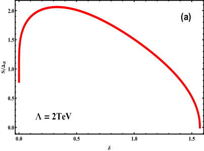
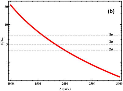
Figure 5: Analysis of the significance $\mathcal{Z}_{4}\!=S/\Delta_{B}$. Plot (a) depicts $\mathcal{Z}_{4}$ as a function of $\,\delta$ . Plot (b) presents $\,\mathcal{Z}_{4}$  for $\,\delta=\delta_{\text{m}}$  as a function of the new physics scale $\Lambda$ .  For illustration, we choose the collision energy $\sqrt{s\,}=3\,\text{TeV}$ and the integrated luminosity $\,\mathcal{L}=2\,\text{ab}^{-1}$.

We present in Fig. 5 the signal significance obtained in this way for the collision energy $\sqrt{s}=3$ TeV. We input the total leptonic branching fraction $\text{Br}(Z\!\rightarrow\!\ell^{-}\ell^{+})\simeq 0.10$,  and assume an integrated luminosity $\mathcal{L}=2\,\text{ab}^{-1}$ and an ideal detection efficiency $\,\epsilon=1\,$ for simplicity. In Fig. 5(a), we depict the significance $\,\mathcal{Z}_{4}$  as a function of the angular cut $\delta$, which exhibits the maximum at $\,\delta_{\text{m}}\simeq 0.33$  for $\Lambda=1$ TeV,  as expected. Thus, under the angular cuts $\,(\phi_{c},\,\delta)\!=(\phi_{\text{c}}^{\text{m}},\,\delta_{\text{m}})$,  we derive

$$(\sigma^{0}_{c},\,\mathbb{O}^{1}_{c}) \simeq \left(23.1,\,11.1\!\left(\!\frac{\text{TeV}}{\Lambda}\right)^{\!\!4}\right)\!\text{fb}\,.$$ (29)

For illustration, we may then use Eq.(27) to estimate the signal significance as follows:

$$\mathcal{Z}_{4}\,\simeq\,32.7\!\left(\!\frac{\,\text{TeV}\,}{\Lambda}\!\right)^{\!\!4}\simeq\,5.0\!\left(\!\frac{\,1.60\,\text{TeV}\,}{\Lambda}\!\right)^{\!\!4},$$ (30)

which is plotted in Fig. 5(b). From this, we find that the probe of the new physics scale can reach $\,\Lambda=(2.0,\,1.8,\,1.6)$ TeV at $(2\sigma,\,3\sigma,\,5\sigma)$ level, respectively.

We note that the practical detection efficiency would be smaller than 100%, so the actual sensitivity may be somewhat weaker. But, as we show later in Eqs.(40) and (44) of Section 3.3, the sensitivity reach for $\Lambda$ has rather weak dependences on the integrated luminosity and detection efficiency, namely, $\,\Lambda\propto(\mathcal{L}\,\epsilon)^{\frac{1}{8}}\,$ at ${\cal O}(\Lambda^{-4})$ and $\,\Lambda\propto(\mathcal{L}\,\epsilon)^{\frac{1}{16}}\,$ at ${\cal O}(\Lambda^{-8})$. Hence, increasing $\,\mathcal{L}\,$ or $\,\epsilon\,$ only has minor effect on the sensitivity reach of the new physics scale $\Lambda$. In contrast, raising the collision energy $\sqrt{s\,}$ can do more to improve the sensitivity reach of $\Lambda$ because $\,\Lambda\propto(\!\sqrt{s\,})^{\frac{1}{2}}\,$ at ${\cal O}(\Lambda^{-4})$ and $\,\Lambda\propto(\!\sqrt{s\,})^{\frac{5}{8}}\,$ at ${\cal O}(\Lambda^{-8})$.

3.2.2 . Analysis Including the ${\cal O}(\Lambda^{\!-8})$ Contribution

In this subsection, we present an analysis to include the contribution of ${\cal O}(\Lambda^{\!-8})$ without invoking strong cancellation on it. Since the ${\cal O}(\Lambda^{\!-8})$ term has a higher power of energy dependence, it may have better sensitivity when the collision energy is higher, e.g., $\sqrt{s}=3$ TeV, even though it is suppressed by $\Lambda^{\!-8}$.  In effective theory analyses considering one operator at time, it is the customary to compute the full  $|\text{amplitude}|^{2}$ including both the interference term with the SM and the squared term of the effective operator when calculating the cross section. In this way the full information concerning a single effective operator is retained.

We see from Fig. 4 that both the distributions $f_{\phi^{*}}^{0}$ and $f_{\phi^{*}}^{2}$ are rather flat. Thus it is hard to discriminate the ${\cal O}(\Lambda^{\!-8})$ contribution from the $\phi_{*}$ distributions. Hence, in order to enhance the signal sensitivity to the ${\cal O}(\Lambda^{\!-8})$ contribution, we study instead the distributions in $\theta$ and $\theta_{*}$. For this, we choose the region $\,\theta\in[\delta,\pi\!-\delta]$  and $\,\theta_{*}\!\in[\delta_{*},\pi\!-\delta_{*}]$.  With the angular cuts $(\delta,\,\delta_{*})$, we compute the SM contribution $\,\sigma_{c}^{0}(Z\gamma)$,  the ${\cal O}(\Lambda^{-4})$ contribution $\,\sigma_{c}^{1}(Z\gamma)$,  and the ${\cal O}(\Lambda^{-8})$ contribution $\,\sigma_{c}^{2}(Z\gamma)\,$ as follows:

$$\sigma_{c}^{0}(Z\gamma) = \frac{\,e^{4}\!\left(8s_{W}^{4}\!-\!4s_{W}^{2}\!+\!1\right)\,}{\,32\pi s_{W}^{2}c_{W}^{2}\!\left(s\!-\!M_{Z}^{2}\right)\!s^{2}\,}\!\times\!\frac{1}{16}\!\left[4\cos\!\delta\left(9\cos\!\delta_{*}\!-\cos\!3\delta_{*}\right)\!M_{Z}^{2}\,s\,\right.$$

$$\hskip 5.69054pt\left.-\left(15\cos\!\delta_{*}\!+\cos\!3\delta_{*}\right)\!(s^{2}\!+\!M_{Z}^{4})\!\!\left(\!\!\cos\!\delta\!+\!2\ln\tan\!\frac{\delta}{2}\right)\!\right]\!,\hskip 28.45274pt$$

$$\sigma^{1}_{c}(Z\gamma) = \pm\frac{\,e^{2}(1\!-\!4s_{W}^{2})M_{Z}^{2}\!\left(s\!-\!M_{Z}^{2}\right)\,}{32\pi s_{W}c_{W}\Lambda^{\!4}s^{2}}\frac{\,\left[2(5\!-\!\cos\!2\delta_{*})s\!+\!\left(\cos\!2\delta_{*}\!\!+\!7\right)\!M_{Z}^{2}\right]\!\cos\!\delta\!\cos\!\delta_{*}\,}{8},\hskip 42.67912pt$$ (31b)

$$\sigma_{c}^{2}(Z\gamma) = \frac{\,\left(8s_{W}^{4}\!-\!4s_{W}^{2}\!+\!1\right)\!M_{Z}^{2}\!\left(s\!-\!M_{Z}^{2}\right)^{\!3}\,}{192\pi\Lambda^{\!8}s^{2}}$$

$$\times\frac{\,\cos\!\delta\,}{64}\!\left[(7\!+\!\cos\!2\delta)\!\left(9\cos\!\delta_{*}\!-\!\cos\!3\delta_{*}\!\right)\!s\!+\!(5\!-\!\cos\!2\delta)\!\left(15\cos\!\delta_{*}\!+\!\cos\!3\delta_{*}\right)\!M_{Z}^{2}\right]\!,$$

where the $\pm$ signs of the ${\cal O}(\Lambda^{\!-4})$ term correspond to the two possible signs of a given dimension-8 operator, $\text{sign}(c_{j})=\pm$,  as shown in Eq.(1). If we take the limit $(\delta,\,\delta_{*})\!\rightarrow\!0$  in the above formulas, we find that they reduce consistently to Eq.(15), as expected.

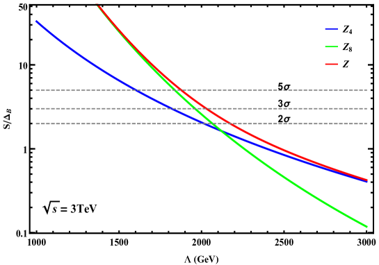
Figure 6: The significance $\,\mathcal{Z}_{8}\!=S/\!\Delta_{B}$  is presented as a function of $\,\Lambda\,$ as a green curve for the cut parameters $(\delta,\,\delta_{*})=(\delta_{m},\,\delta_{*m})$.  The significance $\,\mathcal{Z}_{4}$ [from Fig. 5(a)] is shown as the blue curve for comparison. The combined significance $\,\mathcal{Z}\!=\!\sqrt{\mathcal{Z}_{4}^{2}\!+\!\mathcal{Z}_{8}^{2}\,}$  is depicted by the red curve. For illustration, we choose $\sqrt{s\,}=3\,\text{TeV}$ and $\,\mathcal{L}=2\,\text{ab}^{-1}$.

We can then estimate the corresponding signal significance to be

$$\mathcal{Z}_{8}=\frac{|S_{II}|}{\,\Delta_{B_{II}}\,}=\frac{\,|\sigma_{c}^{1}(Z\gamma)\!+\!\sigma_{c}^{2}(Z\gamma)|\,}{\!\sqrt{\sigma_{c}^{0}(Z\gamma)\,}\,}\!\times\!\sqrt{\text{Br}(Z\!\!\rightarrow\!\ell\ell)\!\times\!\mathcal{L}\!\times\!\epsilon\,}\,.$$ (32)

For comparison with our two-bin analysis of $\mathcal{Z}_{4}$ in Sec. 3.2.1, we could use the same definition of the two bins (regions), (a) and (b), for the $\phi_{*}$ distribution (Fig. 4), as given above Eq.(23). But, the signal and background cross sections in Eq.(32) correspond to integrating the distributions $f_{\phi_{*}}^{j}$ ($j=0,1,2$) over the full range of $\,\phi_{*}\in[0,\,2\pi)$,  for which all the $\cos\!\phi_{*}$ and $\cos\!2\phi_{*}$ terms vanish and only the constant terms $\,\frac{1}{2\pi}\,$ in Eq.(21) survive. This means that we sum up the two bins (a) and (b), rather than taking the difference of the two bins (as we did for $\mathcal{Z}_{4}$ in Sec. 3.2.1). Namely, the current signal $S_{II}$, the SM background $B_{II}$ and its statistical error $\Delta_{B_{II}}$ take the following forms,

$$S_{II} = \left[\sigma_{c}^{1}(Z\gamma)\!+\!\sigma_{c}^{2}(Z\gamma)\right]\!\times\!\left[\text{Br}(Z\!\!\rightarrow\!\ell\ell)\!\times\!\mathcal{L}\!\times\!\epsilon\right]=\overline{N}_{\!12}^{a}+\overline{N}_{\!12}^{b}\,,$$ (33a)

$$B_{II} = \sigma_{c}^{0}(Z\gamma)\!\times\!\left[\text{Br}(Z\!\!\rightarrow\!\ell\ell)\!\times\!\mathcal{L}\!\times\!\epsilon\right]=\overline{N}_{0}^{a}+\overline{N}_{0}^{b}\,,$$ (33b)

$$\Delta_{B_{II}}\! = \!\sqrt{B_{II}}=(\overline{N}_{0}^{a}+\overline{N}_{0}^{b})^{\!{1}/{2}}\,\,.$$ (33c)

Here $(\overline{N}_{\!12}^{a},\,\overline{N}_{\!12}^{b})$ denote the signal event numbers in the regions (a) and (b) of the distributions $f_{\phi_{*}}^{1,2}$,  in which only the constant terms $1/(2\pi)$ contribute to the sum $\,\overline{N}_{\!12}^{a}\!+\!\overline{N}_{\!12}^{b}$ under the uniform integration over full range of $\phi_{*}$.  Also, $\overline{N}_{0}^{a}\!+\!\overline{N}_{0}^{b}$ denotes the sum of the background event numbers in the regions (a) and (b) of the distribution $f_{\phi_{*}}^{0}$.  (Here our notations of the background event numbers $(\overline{N}_{0}^{a},\,\overline{N}_{0}^{b})$ differ from $({N}_{0}^{a},\,{N}_{0}^{b})$ in the other independent analysis of Sec. 3.2.1 because we have added different $\theta$ cuts separately for the two analyses in Sec. 3.2.1 and Sec. 3.2.2.)

To obtain the maximal signal significance, we derive the corresponding values of the angular cuts $(\delta,\,\delta_{*})=(\delta_{\text{m}},\,\delta_{*\text{m}})$, which are $(\delta_{\text{m}},\,\delta_{*\text{m}})\simeq(0.623,\,0.820)$. Inputting $\,\text{Br}(Z\!\!\rightarrow\!\ell\ell)\!\simeq 0.10$  and choosing $\sqrt{s}=3\,$TeV, $\mathcal{L}=2\,\text{ab}^{-1}$ and $\epsilon=1$,  we compute the cross section for $Z\gamma$ production:

$$\sigma(Z\gamma)=\left[10.1\pm 0.0251\!\left(\!\frac{\,2\text{TeV}\,}{\Lambda}\!\right)^{\!\!4}+0.554\!\left(\!\frac{\,2\text{TeV}\,}{\Lambda}\!\right)^{\!\!8}\right]\!\text{fb}\,.$$ (34)

Thus, from Eq.(32) we estimate the signal significance

$$\mathcal{Z}_{8}\simeq\,\left|\pm 1.79\!\left(\!\frac{\,\text{TeV}\,}{\Lambda}\!\right)^{\!\!4}+631\!\left(\!\frac{\,\text{TeV}\,}{\Lambda}\!\right)^{\!\!8}\right|\,\simeq\,\left|\pm 0.112\!\left(\!\frac{\,2\,\text{TeV}\,}{\Lambda}\!\right)^{\!\!4}+2.46\!\left(\!\frac{\,2\,\text{TeV}\,}{\Lambda}\!\right)^{\!\!8}\right|\!.\hskip 34.1433pt$$ (35)

We see that for the collision energy $\sqrt{s}=3\,$TeV, the ${\cal O}(\Lambda^{\!-8})$ term dominates the sensitivity.

In Appendix B, we have systematically proven that the possible correlation between the two significances $\mathcal{Z}_{4}$ and $\mathcal{Z}_{8}$ are fully negligible. Hence, it is well justified to combine $\mathcal{Z}_{4}$  and $\,\mathcal{Z}_{8}$  for achieving an improved sensitivity reach to the new physics scale $\Lambda$ ,

$$\mathcal{Z}=\!\sqrt{\mathcal{Z}_{4}^{2}\!+\!\mathcal{Z}_{8}^{2}\,}\,.\,$$ (36)

This is depicted by the red curve in Fig. 6. In this way, we find that the new physics scale can be probed up to $\,\Lambda\simeq(2.2,\,2.0,\,1.9)$ TeV at the $(2\sigma,\,3\sigma,\,5\sigma)$ levels, respectively. These numbers apply for both $\pm$ signs in Eq.(35), since we find that the case of minus sign in Eq.(35) only causes a tiny difference in the $\Lambda$ bound by less than 1%. Hence, the ${\cal O}(\Lambda^{\!-4})$ term in Eq.(35) has negligible effect for the collider energy $\sqrt{s\,}=3$ TeV.  As we will show in Section 3.2.3, this feature applies to all cases with $\sqrt{s\,}\gtrsim 1$ TeV.

$\sqrt{s\,}$ (GeV)	250	500	1000	3000	5000
$\mathcal{Z}_{4}\!:~{}(\delta_{\text{m}}^{(4)},\,\phi_{c}^{\text{m}})$	(0.368, 1.17)	(0.340, 1.17)	(0.332, 1.17)	(0.329, 1.17))	(0.329, 1.17)
$\mathcal{Z}_{8}\!:~{}(\delta_{\text{m}}^{(8)},\,\delta_{*\text{m}})$	(0.608, 0.692)	(0.616, 0.790)	(0.621, 0.814)	(0.623, 0.820)	(0.623, 0.821)

Table 1: Summary of the optimal angular cuts for realizing the maximal signal significance. For the signal significance $\mathcal{Z}_{4}$, we impose the cuts $(\delta_{\text{m}}^{(4)},\,\phi_{c}^{\text{m}})$ on the angular distributions of $(\theta,\,\phi_{*})$; whereas for the signal significance $\mathcal{Z}_{8}$, we set the cuts $(\delta_{\text{m}}^{(8)},\,\delta_{*\text{m}})$ on the angular distributions of $(\theta,\,\theta_{*})$.  These cuts correspond to the allowed angular ranges, $\delta_{\text{m}}\!<\theta<\pi-\delta_{\text{m}}$,  $\delta_{*\text{m}}\!<\!\theta_{*}\!<\pi\!-\delta_{*\text{m}}$,  and $\,\phi\in\left[0,\,\phi_{c}^{\text{m}}\right]\bigcup\left[2\pi\!-\!\phi_{c}^{\text{m}},\,2\pi\right)\bigcup\left[\pi\!-\!\phi_{\text{c}},\,\pi\!+\!\phi_{\text{c}}\right]$,  where $\delta_{\text{m}}\!=\!\delta_{\text{m}}^{(4)}\!$ or $\delta_{\text{m}}^{(8)}$.

3.2.3 . Analysis of Different Collision Energies

In this subsection, we further extend our analysis of $\sqrt{s\,}\!=\!3$ TeV case to different collision energies $\sqrt{s\,}\!=(250,\,500,\,1000,\,5000)$ GeV, in each case with a sample integrated luminosity $\mathcal{L}=2\,\text{ab}^{-1}$.

Using the same method as we presented in Section 3.2.1-3.2.2, we analyze the SM backgrounds and signal contributions for different collider energies. For each given collider energy $\sqrt{s\,}$,  we derive the optimal angular cuts for realizing the maximal signal significance $\mathcal{Z}_{4}$ and $\mathcal{Z}_{8}$.  Namely, for the analysis of $\mathcal{Z}_{4}$, we use the angular cuts $(\delta_{\text{m}},\,\phi_{c}^{\text{m}})$ for angles $(\theta,\,\phi_{*})$;  while for the analysis of $\mathcal{Z}_{8}$, we use the angular cuts $(\delta_{\text{m}},\,\delta_{*\text{m}})$ for angles $(\theta,\,\theta_{*})$.  We summarize the optimal angular cuts for different collider energies in Table 1. As we noted below Eq.(28), the dominant contribution to the signal significance $\mathcal{Z}_{4}$ depends on the cut $\phi_{c}$ only through a simple function $\,\sin\phi_{\text{c}}/\!\sqrt{\phi_{\text{c}}}$ ,  which does not depend on energy $\!\sqrt{s\,}$ and reaches its maximum at $\phi_{c}^{\text{m}}\simeq 1.17$.  This is why the optimal cut $\phi_{c}^{\text{m}}$ is nearly independent of the collider energy $\sqrt{s\,}$, as shown in Table 1. Here, for the $\delta_{\text{m}}$ cut, we have added the superscript to $\delta_{\text{m}}^{(4)}$ for $\mathcal{Z}_{4}$ and the superscript to $\delta_{\text{m}}^{(8)}$ for $\mathcal{Z}_{8}$, to indicate that the two cuts $\delta_{\text{m}}^{(4)}$ and $\delta_{\text{m}}^{(8)}$ are imposed (optimized) for the observables of $\mathcal{Z}_{4}$ and $\mathcal{Z}_{8}$ separately and independently. We note that this $\theta$ cut is a type of basic selection cuts. Table 1 shows that the optimized $\theta$ cut has little change when the collider energy $\!\sqrt{s\,}$ varies from 250 GeV all the way up to 5 TeV for the analysis of either $\mathcal{Z}_{4}$ or $\mathcal{Z}_{8}$.  In fact, the angular $\theta$ cuts in Table 1 cannot cause any correlation between $\mathcal{Z}_{4}$ and $\mathcal{Z}_{8}$.  This is fully clarified in Appendix B.

With the optimal kinematical cuts in Table 1, we compute the SM contributions and the ${\cal O}(\Lambda^{-4})$ contributions for different collider energies,

$$\sqrt{s}=250\,\text{GeV}, (\sigma^{0}_{c},\,\mathbb{O}^{1}_{c})=\left(\!3936,\,0.913\!\left(\!\frac{\text{TeV}}{\Lambda}\right)^{\!\!4}\right)\!\text{fb}\,,\hskip 34.1433pt$$ (37a)

$$\sqrt{s}=500\,\text{GeV}, (\sigma^{0}_{c},\,\mathbb{O}^{1}_{c})=\left(\!860,\,1.85\!\left(\!\frac{\text{TeV}}{\Lambda}\right)^{\!\!4}\right)\!\text{fb}\,,$$ (37b)

$$\sqrt{s}=1\,\text{TeV}, (\sigma^{0}_{c},\,\mathbb{O}^{1}_{c})=\left(\!209,\,3.71\!\left(\!\frac{\text{TeV}}{\Lambda}\right)^{\!\!4}\right)\!\text{fb}\,,$$ (37c)

$$\sqrt{s}=3\,\text{TeV}, (\sigma^{0}_{c},\,\mathbb{O}^{1}_{c})=\left(\!23.1,\,11.1\!\left(\!\frac{\text{TeV}}{\Lambda}\right)^{\!\!4}\right)\!\text{fb}\,,$$ (37d)

$$\sqrt{s}=5\,\text{TeV}, (\sigma^{0}_{c},\,\mathbb{O}^{1}_{c})=\left(\!8.30,\,18.5\!\left(\!\frac{\text{TeV}}{\Lambda}\right)^{\!\!4}\right)\!\text{fb}\,,$$ (37e)

where we include the case of $\sqrt{s}=3$ TeV from Eq.(29) for comparison.

With these, we derive the following signal significances at each collision energy, for the leptonic branching fraction $\,\text{Br}(Z\!\!\rightarrow\!\ell\ell)\!\simeq 0.10$  and an integrated luminosity $\mathcal{L}=2\,\text{ab}^{-1}$:

$$\sqrt{s}=250\,\text{GeV}, \mathcal{Z}_{4}=\,3.29\!\left(\!\frac{\,0.5\text{TeV}\,}{\Lambda}\!\right)^{\!\!4}\!\times\!\sqrt{\epsilon\,}\,,\hskip 34.1433pt$$ (38a)

$$\sqrt{s}=500\,\text{GeV}, \mathcal{Z}_{4}=\,2.18\!\left(\!\frac{\,0.8\text{TeV}\,}{\Lambda}\!\right)^{\!\!4}\!\times\!\sqrt{\epsilon\,}\,,$$ (38b)

$$\sqrt{s}=1\,\text{TeV}, \mathcal{Z}_{4}=\,3.62\!\left(\!\frac{\,\text{TeV}\,}{\Lambda}\!\right)^{\!\!4}\!\times\!\sqrt{\epsilon\,}\,,$$ (38c)

$$\sqrt{s}=3\,\text{TeV}, \mathcal{Z}_{4}\,\simeq\,2.05\!\left(\!\frac{\,2\text{TeV}\,}{\Lambda}\!\right)^{\!\!4}\!\times\!\sqrt{\epsilon\,}\,,$$ (38d)

$$\sqrt{s}=5\,\text{TeV}, \mathcal{Z}_{4}=\,2.33\!\left(\!\frac{\,2.5\text{TeV}\,}{\Lambda}\!\right)^{\!\!4}\!\times\!\sqrt{\epsilon\,}\,.$$ (38e)

We note that the signal significance is nearly proportional to the squared centre-of-mass collision energy $\,(\!\sqrt{s\,})^{2}\,$.  At high energies $s\!\gg\!M_{Z}^{2}$, we have

$$\mathcal{Z}_{4}\propto\frac{M_{Z}\,s}{\,\Lambda^{4}\,}\sqrt{\mathcal{L}\!\times\!\epsilon\,}\,.$$ (39)

Thus, for a given significance $\mathcal{Z}_{4}$, the corresponding reach of the new physics scale $\Lambda$ is

$$\Lambda\propto\left(\!\frac{\,M_{Z}\sqrt{\mathcal{L}\!\times\!\epsilon\,}\,}{\,\mathcal{Z}_{4}}\right)^{\!\!\!\frac{1}{4}}\!\!\times\!\left(\!\sqrt{s\,}\right)^{\!\frac{1}{2}}.$$ (40)

We see that the collision energy $\sqrt{s\,}$  has the most sensitive effect on the reach of the new physics scale $\Lambda$ .  For instance, raising the collision energy from $\,\sqrt{s\,}=250$ GeV to $\sqrt{s\,}=3$ TeV, the reach of the new physics scale is improved by a significant factor $\,\Lambda(3~{}\text{TeV})/\Lambda(250~{}\text{GeV})\simeq 3.46\,$.  On the other hand, $\Lambda$ has a rather weak dependence on the significance, $\,\Lambda\propto\mathcal{Z}_{4}^{-\frac{1}{4}}\,$,  so the $5\sigma$ reach is only slightly weaker than the $2\sigma$ reach: $\Lambda(5\sigma)/\Lambda(2\sigma)\simeq 1/1.26$ . Furthermore, we note that $\Lambda$ depends much more weakly on the integrated luminosity and the detection efficiency, $\,\Lambda\propto(\mathcal{L}\!\times\!\epsilon)^{\frac{1}{8}}$.  For instance, increasing the integrated luminosity from $\mathcal{L}=2\,\text{ab}^{-1}$ to $\mathcal{L}=6\,\text{ab}^{-1}$, would enhance the reach of the new physics scale by only a factor of $\,\Lambda(6\text{ab}^{-1})/\Lambda(2\text{ab}^{-1})\simeq 1.15$ .  Also, if the detection efficiency is increased from $\,\epsilon=40\%$  to  $\epsilon=90\%$,  the reach of the new physics scale would be only slightly extended by a factor of $\,\Lambda(90\%)/\Lambda(40\%)\simeq 1.11$ .

Next, extending Section 3.2.2 to different collision energies, we include contributions up to ${\cal O}(\Lambda^{\!-8})$ in a similar manner. We apply the optimal kinematical cuts as in Table 1 and compute the cross sections of $\,e^{+}e^{-}\!\!\rightarrow\!Z\gamma$  as follows:

$$\sqrt{s\,}\!=250~{}\text{GeV}, \sigma(Z\gamma)=\left[2427\pm 6.62\!\left(\!\frac{\,0.5\text{TeV}\,}{\Lambda}\!\right)^{\!\!4}\!+1.39\!\left(\!\frac{\,0.5\text{TeV}\,}{\Lambda}\!\right)^{\!\!8}\right]\!\text{fb}\,,~{}~{}~{}~{}~{}~{}~{}~{}$$ (41a)

$$\sqrt{s\,}\!=500~{}\text{GeV}, \sigma(Z\gamma)=\left[417\pm 0.996\!\left(\!\frac{\,0.8\text{TeV}\,}{\Lambda}\!\right)^{\!\!4}\!+0.624\!\left(\!\frac{\,0.8\text{TeV}\,}{\Lambda}\!\right)^{\!\!8}\right]\!\text{fb}\,,$$ (41b)

$$\sqrt{s\,}\!=1~{}\text{TeV}, \sigma(Z\gamma)=\left[94.0\pm 0.404\!\left(\!\frac{\,\text{TeV}\,}{\Lambda}\!\right)^{\!\!4}+1.73\!\left(\!\frac{\,\text{TeV}\,}{\Lambda}\!\right)^{\!\!8}\right]\!\text{fb}\,,$$ (41c)

$$\sqrt{s\,}\!=3~{}\text{TeV}, \sigma(Z\gamma)=\left[10.1\pm 0.0252\!\left(\!\frac{\,2\text{TeV}\,}{\Lambda}\!\right)^{\!\!4}+0.554\!\left(\!\frac{\,2\text{TeV}\,}{\Lambda}\!\right)^{\!\!8}\right]\!\text{fb}\,,$$ (41d)

$$\sqrt{s\,}\!=5~{}\text{TeV}, \sigma(Z\gamma)=\left[3.63\pm 0.0103\!\left(\!\frac{\,2.5\text{TeV}\,}{\Lambda}\!\right)^{\!\!4}+0.718\!\left(\!\frac{\,2.5\text{TeV}\,}{\Lambda}\!\right)^{\!\!8}\right]\!\text{fb}\,,~{}~{}~{}~{}~{}~{}~{}~{}~{}~{}$$ (41e)

where for comparison we have also included the result from Eq.(34) for the case of $\sqrt{s\,}\!=3\,\text{TeV}$.  The above can be compared to the cross sections (16) with only a preliminary angular cut $\,\delta>0.2$  (corresponding to a lower cut on the photon transverse momentum $\,P_{T}^{\gamma}=q\sin\delta$ ). We see that under the final angular cuts on $(\theta,\,\theta_{*},\,\phi_{*})$ the SM contribution is substantially reduced in each case, whereas the signal contributions at ${\cal O}(\Lambda^{\!-4})$ and ${\cal O}(\Lambda^{\!-8})$ are little changed.

Uisng the above, we analyze the signal significance up to ${\cal O}(\Lambda^{\!-8})$,  for different collider energies. With inputs of the leptonic branching fraction $\,\text{Br}(Z\!\!\rightarrow\!\ell\ell)\!\simeq 0.10$  and an integrated luminosity $\mathcal{L}\!=\!2\,\text{ab}^{-1}$,  we arrive at

$$\sqrt{s}=250\,\text{GeV}, \mathcal{Z}_{8}=\left|\pm 1.90\!\left(\!\frac{\,0.5\text{TeV}\,}{\Lambda}\!\right)^{\!\!4}+0.400\!\left(\!\frac{\,0.5\text{TeV}\,}{\Lambda}\!\right)^{\!\!8}\right|\!\times\!\sqrt{\epsilon\,}\,,\hskip 71.13188pt$$ (42a)

$$\sqrt{s}=500\,\text{GeV}, \mathcal{Z}_{8}=\left|\pm 0.689\left(\!\frac{\,0.8\text{TeV}\,}{\Lambda}\!\right)^{\!\!4}+0.432\!\left(\!\frac{\,0.8\text{TeV}\,}{\Lambda}\!\right)^{\!\!8}\right|\!\times\!\sqrt{\epsilon\,}\,,$$ (42b)

$$\sqrt{s}=1\,\text{TeV}, \mathcal{Z}_{8}=\left|\pm 0.589\!\left(\!\frac{\,\text{TeV}\,}{\Lambda}\!\right)^{\!\!4}+2.53\!\left(\!\frac{\,\text{TeV}\,}{\Lambda}\!\right)^{\!\!8}\right|\!\times\!\sqrt{\epsilon\,}\,,$$ (42c)

$$\sqrt{s}=3\,\text{TeV}, \mathcal{Z}_{8}=\left|\pm 0.112\!\left(\!\frac{\,2\,\text{TeV}\,}{\Lambda}\!\right)^{\!\!4}+2.46\!\left(\!\frac{\,2\,\text{TeV}\,}{\Lambda}\!\right)^{\!\!8}\right|\!\times\!\sqrt{\epsilon\,}\,,$$ (42d)

$$\sqrt{s}=5\,\text{TeV}, \mathcal{Z}_{8}=\left|\pm 0.0764\!\left(\!\frac{\,2.5\text{TeV}\,}{\Lambda}\!\right)^{\!\!4}+5.32\!\left(\!\frac{\,2.5\text{TeV}\,}{\Lambda}\!\right)^{\!\!8}\right|\!\times\!\sqrt{\epsilon\,}\,.$$ (42e)

From the above, we note that for the relevant reach of $\,\Lambda$ ,  the ${\cal O}(\Lambda^{\!-4})$ terms give the dominant contributions for collision energies $\sqrt{s}<\!1$ TeV,  while the ${\cal O}(\Lambda^{\!-8})$ terms become dominant for $\sqrt{s}\gtrsim\!1$ TeV.  When ${\cal O}(\Lambda^{\!-8})$ becomes dominant at high energies, we have $\,\Lambda\propto\mathcal{Z}_{8}^{-\frac{1}{8}}$.  In such cases, the reach in $\Lambda$ becomes rather insensitive to the significance $\mathcal{Z}_{8}$.  For instance, at high energies $\sqrt{s}\gtrsim\!1$ TeV,  we have $\Lambda(5\sigma)/\Lambda(2\sigma)\simeq 1/1.12$  for $\mathcal{Z}_{8}$,  whereas we previously found $\Lambda(5\sigma)/\Lambda(2\sigma)\simeq 1/1.26$  for $\mathcal{Z}_{4}$.

At high energies $\,s\gtrsim(1\text{TeV})^{2}\gg\!M_{Z}^{2}$,  the ${\cal O}(\Lambda^{\!-8})$ terms become dominant, so we have the approximate relation

$$\mathcal{Z}_{8}\propto\frac{\,M_{Z}^{2}(\!\sqrt{s\,})^{5}\,}{\,\Lambda^{8}\,}\sqrt{\mathcal{L}\!\times\!\epsilon\,}\,,$$ (43)

and hence

$$\Lambda\,\propto\,\left(\!\!\frac{\,M_{Z}^{2}\sqrt{\mathcal{L}\,\epsilon\,}\,}{\,\mathcal{Z}_{8}\,}\!\right)^{\!\!\!\frac{1}{8}}\!\left(\!\sqrt{s\,}\right)^{\!\frac{5}{8}}.$$ (44)

We see from Eqs.(40) and (44) that the sensitivity to $\Lambda$ increases with the collision energy with the power $\!(\!\sqrt{s\,})^{\frac{1}{2}}$ or $\!(\!\sqrt{s\,})^{\frac{5}{8}}$,  a relatively slow rate of increase. We note also that the sensitivity to the new physics scale $\Lambda$ is rather insensitive to the integrated luminosity $\mathcal{L}$ and the detection efficiency $\,\epsilon\,$, owing to their small power-law dependence $\left(\mathcal{L}\,\epsilon\right)^{\!\frac{1}{16}}$.

$\sqrt{s}$ (GeV)	250	500	1000	3000	5000
$\Lambda_{2\sigma}$ (TeV)	0.59(0.58)	0.84(0.82)	1.2	2.2	2.9
$\Lambda_{5\sigma}$ (TeV)	0.48(0.46)	0.68(0.65)	1.0	1.9	2.6

Table 2: Combined sensitivity reaches to the new physics scale $\Lambda$ at the $2\sigma$ and $5\sigma$ levels, for different collider energies. Here the two numbers in the parentheses correspond to the case of the dimension-8 operator whose coefficient has a minus sign, while in all other entries the effects due to the coefficient having a minus sign are negligible. For illustration, we have input a fixed representative integrated luminosity $\,\mathcal{L}=2\,\text{ab}^{-1}\!$ and an ideal detection efficiency $\,\epsilon=100\%$.

Finally, we compute from Eqs.(38) and (42), the combined significance, $\mathcal{Z}\!=\sqrt{\mathcal{Z}_{4}^{2}\!+\!\mathcal{Z}_{8}^{2}\,}$,  for each collider energy. With these, in Table 2 we present the corresponding combined sensitivity reaches to the new physics scale $\Lambda$ at different $e^{+}e^{-}$ collider energies. In the last row of this Table, the two numbers in the parentheses correspond to the case of the dimension-8 operator whose coefficient has a minus sign, whereas in all other entries the effects due to the coefficient having a minus sign are negligible. Note also that in current analysis we have chosen a universal integrated luminosity $\,\mathcal{L}=2\,\text{ab}^{-1}\!$ for illustration. But it is straightforward to obtain the significance $\mathcal{Z}$ for any other given integrated luminosity $\,\mathcal{L}\,$ by a simple rescaling due to $\,\mathcal{Z}\!\propto\!\sqrt{\!\mathcal{L}\,}$.

Before concluding this Section, we mention that we have performed a numerical Monte Carlo simulation based on the analytical formula (28). We used for this purpose CUDAlink in Mathematica, so as to exploit the CUDA parallel computing architecture on Graphical Processing Units (GPUs), which can generate millions of events in seconds. We have computed the probability density function of $\theta$, $\theta_{*}$ and $\phi_{*}$ for the case of $\sqrt{s\,}=3\,$TeV and $\Lambda=2$ TeV. Eq.(16d) shows that the SM contribution dominates the total cross section. According to Eq.(29), we have $\,\mathbb{O}_{1}^{c}/\sigma_{0}^{c}\simeq 0.03$ .  For comparison, our Monte Carlo simulation yielded the following event counts: $\,|N_{a}\!-\!N_{b}|=3054$ and $\,N_{a}\!+\!N_{b}=104752$, corresponding to $\,|N_{a}\!-\!N_{b}|/(N_{a}\!+\!N_{b})\simeq 0.029$.  This agrees well with the ratio $\mathbb{O}_{1}^{c}/\sigma_{0}^{c}\simeq 0.03$ inferred from our analytical formula (28), serving as a consistency check on our Eq.(29). Our Monte Carlo simulation package may be used to generate other distributions and quantities that may be of interest for experiments.

In passing, we note that subsequent to Refs. nTGC1 ; Degrande:2013kka some other follow-up studies discussed testing nTGCs at ILC(800GeV) India1 and ILC(500GeV) India2 using the form factors for the nTGC nTGC1 . Unlike Refs. India1 India2 , we study the fully gauge-invariant dimension-8 operators (2) for the nTGCs which are much more restrictive and result in just one independent operator $\mathcal{O}_{\widetilde{B}W}$. Only the gauge-invariant formulation of nTGCs via dimension-8 operators can identify the power-dependence on the associated UV cutoff $\Lambda$, making possible the probe of the new physics scale $\Lambda$ . We perform a systematic study and comparison, probing the sensitivity to $\Lambda$ of nTGC measurements at different collider energies and covering all future $e^{+}e^{-}$ colliders being planned, including CEPC, FCCee, ILC and CLIC, rather than studying only a specific collider energy (800GeV India1 or 500GeV India2 ). Our independent study presents the complete angular distributions both analytically and numerically for all future $e^{+}e^{-}$ colliders, which allow us to construct the angular observables in Sec. 3.1. Refs. India1 India2 considered some angular observables, but did not provide any complete angular distributions. In particular, they did not show any $\phi_{*}$ distributions, and they also did not give any analytical formulas for angular differential cross sections. Hence, it is difficult to compare with our independent work even for the special collider energy 500 GeV. We study systematically the impact of $e^{\mp}$ beam polarizations on probing the new physics scale of nTGCs in Sec. 5, unlike Ref. India2 , which did not consider the beam polarizations. We study both leptonic $Z$-decays (Sec. 3 and 5) and invisible $Z$-decays (Sec. 4 and 5). Ref. India1 even did not consider the final state $Z$-decays for a realistic analysis of signals and backgrounds, while India2 did not study the invisible $Z$-decay channels.

3.3 . Non-Resonant Backgrounds

Figure 7: Five types of Feynman diagrams which contribute to the process $e^{-}e^{+}\!\!\rightarrow\!\!f\bar{f}\gamma$  (with $f\!=\!\ell,\nu$). Type (a) is our signal with a $Z^{*}Z\gamma$ vertex solely from the dimension-8 operator (2a), and types (b),(c),(d),(e) are the SM backgrounds. The type (b) process $\,e^{-}e^{+}\!\!\rightarrow\!V\gamma\!\rightarrow\!\gamma f\bar{f}$  (with $V\!\!=Z,\gamma^{*}$) gives an irreducible background (and there is a similar $u$-channel diagram). Type (c) is $s$-channel gauge boson exchange ($V\!=Z^{*},\gamma^{*}$) with final-state $\gamma$ radiation. Type (d) is $t$-channel $V$ exchange ($V\!\!=\!Z^{*},\gamma^{*}$) with the final-state $\gamma$ radiated from $e^{\pm}$ (in the final or initial state). Type (e) is for the $\nu\bar{\nu}\gamma$ final state with $t$-channel $W^{*}\!$-exchange and the $\gamma$ radiated from either the $W^{*}$ or the initial-state $e^{\pm}$. 

In the analyses so far, we have considered $e^{-}e^{+}\!\!\rightarrow\!Z\gamma$  production with on-shell $Z$ decays ($Z\!\!\rightarrow\!\ell^{-}\ell^{+}$). This means that we have considered only the signal contribution Fig. 7(a) and the irreducible background Fig. 7(b). There are other (non-resonant) SM backgrounds with the same final state of $f\bar{f}\gamma$ ($f\!\!=\!\ell,\nu$), but having very different topology where $\,\gamma$  is radiated either from the final-state fermions [Fig. 7(c)-(d)], or from a $t$-channel $W$ boson [Fig. 7(e)] in the case of $\,Z\!\rightarrow\!\nu\bar{\nu}$  decay (which will be studied in Section 4). These backgrounds may give visible but small contributions after proper kinematic cuts.

For the backgrounds with an $e^{-}e^{+}\gamma$ final state, we have type (b) (with 4 diagrams), type (c) (with 4 diagrams) and type (d) (with 8 diagrams), for a total of 16 diagrams. For the other $f\bar{f}\gamma$ final states with $f=\mu,\tau$, we have type (b) (with 4 diagrams) and type (c) (with 8 diagrams), which amount to 12 diagrams. For the final state $\nu\bar{\nu}\gamma$,  we have the SM backgrounds from type (b)(with 2 diagrams) and type (e) (with 3 diagrams). For each of these diagrams, there are $\,2^{3}\!=8$  helicity combinations. Rather than writing explicitly the cross sections for all these combinations and calculating them analytically, we have computed the cross section numerically using a Monte Carlo method. The relative accuracy of numerical Monte Carlo integration is $\,{O}(1\!/\!\sqrt{\!N})$,  where $N$ is the number of samples, and one needs a large sample to obtain precise results. We use FeynArts Hahn:2000kx to generate all the background diagrams and then compute them by FeynCalc Shtabovenko:2016sxi ; Mertig:1990an . Finally, we convert the expressions to $C$ form and use CUDAlink for numerical integrations to compute the cross sections and other observables. All steps are done in Mathematica and the numerical computation speed is ${O}(10^{7})$ diagrams/$s$.

The diagrams of Fig.7(c)-(d) have additional soft and collinear divergences, which can be removed by imposing lower cuts on the photon transverse momentum $\,P_{T}^{\gamma}>0.2P_{\gamma}$  and on the lepton-photon invariant mass $\,M(\ell\gamma)>0.1\sqrt{s}\,$.  We further require $|M(\ell\ell)\!-\!M_{Z}|\!<\!10$ GeV  so as to be close to the $Z$ boson mass-shell. Applying these cuts together with those in Table 1, we first compute the observables for the reaction channel $e^{-}e^{+}\!\!\rightarrow\!\gamma e^{-}e^{+}$  by including the additional backgrounds in Fig. 7(c)-(d),

$$\sqrt{s}=250\,\text{GeV}, (\sigma^{0e}_{c},\,\mathbb{O}^{1e}_{c})=\left(\!141,\,0.0256\!\left(\!\frac{\text{TeV}}{\Lambda}\right)^{\!\!4}\right)\!\text{fb}\,,\hskip 34.1433pt$$ (45a)

$$\sqrt{s}=500\,\text{GeV}, (\sigma^{0e}_{c},\,\mathbb{O}^{1e}_{c})=\left(\!26.6,\,0.0524\!\left(\!\frac{\text{TeV}}{\Lambda}\right)^{\!\!4}\right)\!\text{fb}\,,$$ (45b)

$$\sqrt{s}=1\,\text{TeV}, (\sigma^{0e}_{c},\,\mathbb{O}^{1e}_{c})=\left(\!6.15,\,0.109\!\left(\!\frac{\text{TeV}}{\Lambda}\right)^{\!\!4}\right)\!\text{fb}\,,$$ (45c)

$$\sqrt{s}=3\,\text{TeV}, (\sigma^{0e}_{c},\,\mathbb{O}^{1e}_{c})=\left(\!0.691,\,0.340\!\left(\!\frac{\text{TeV}}{\Lambda}\right)^{\!\!4}\right)\!\text{fb}\,,$$ (45d)

$$\sqrt{s}=5\,\text{TeV}, (\sigma^{0e}_{c},\,\mathbb{O}^{1e}_{c})=\left(\!0.250,\,0.567\!\left(\!\frac{\text{TeV}}{\Lambda}\right)^{\!\!4}\right)\!\text{fb}\,.$$ (45e)

We then derive the following signal significance $\mathcal{Z}_{4}^{e}$ at each collision energy, assuming an integrated luminosity $\mathcal{L}=2\,\text{ab}^{-1}$:

$$\sqrt{s}=250\,\text{GeV}, \mathcal{Z}_{4}^{e}=\,1.54\!\left(\!\frac{\,0.5\text{TeV}\,}{\Lambda}\!\right)^{\!\!4}\!\times\!\sqrt{\epsilon\,}\,,\hskip 34.1433pt$$ (46a)

$$\sqrt{s}=500\,\text{GeV}, \mathcal{Z}_{4}^{e}=\,1.11\!\left(\!\frac{\,0.8\text{TeV}\,}{\Lambda}\!\right)^{\!\!4}\!\times\!\sqrt{\epsilon\,}\,,$$ (46b)

$$\sqrt{s}=1\,\text{TeV}, \mathcal{Z}_{4}^{e}=\,1.97\!\left(\!\frac{\,\text{TeV}\,}{\Lambda}\!\right)^{\!\!4}\!\times\!\sqrt{\epsilon\,}\,,$$ (46c)

$$\sqrt{s}=3\,\text{TeV}, \mathcal{Z}_{4}^{e}\,=\,1.14\!\left(\!\frac{\,2\text{TeV}\,}{\Lambda}\!\right)^{\!\!4}\!\times\!\sqrt{\epsilon\,}\,,$$ (46d)

$$\sqrt{s}=5\,\text{TeV}, \mathcal{Z}_{4}^{e}=\,1.30\!\left(\!\frac{\,2.5\text{TeV}\,}{\Lambda}\!\right)^{\!\!4}\!\times\!\sqrt{\epsilon\,}\,.$$ (46e)

Next, we extend the analysis of Section 3.2.2 by including the $O(\Lambda^{\!-8})$ contributions and the additional backgrounds in Fig. 7(c)-(d). Thus, we arrive at

$$\sqrt{s\,}\!=250\,\text{GeV}, \sigma(ee\gamma)=\left[85.0\pm 0.20\!\left(\!\frac{\,0.5\text{TeV}\,}{\Lambda}\!\right)^{\!\!4}\!+0.0418\!\left(\!\frac{\,0.5\text{TeV}\,}{\Lambda}\!\right)^{\!\!8}\right]\!\text{fb}\,,~{}~{}~{}~{}~{}~{}~{}~{}$$ (47a)

$$\sqrt{s\,}\!=500\,\text{GeV}, \sigma(ee\gamma)=\left[13.6\pm 0.32\!\left(\!\frac{\,0.8\text{TeV}\,}{\Lambda}\!\right)^{\!\!4}\!+0.0192\!\left(\!\frac{\,0.8\text{TeV}\,}{\Lambda}\!\right)^{\!\!8}\right]\!\text{fb}\,,$$ (47b)

$$\sqrt{s\,}\!=1\,\text{TeV}, \sigma(ee\gamma)=\left[3.03\pm 0.13\!\left(\!\frac{\,\text{TeV}\,}{\Lambda}\!\right)^{\!\!4}+0.0536\!\left(\!\frac{\,\text{TeV}\,}{\Lambda}\!\right)^{\!\!8}\right]\!\text{fb}\,,$$ (47c)

$$\sqrt{s\,}\!=3\,\text{TeV}, \sigma(ee\gamma)=\left[0.325\pm 0.0008\!\left(\!\frac{\,2\text{TeV}\,}{\Lambda}\!\right)^{\!\!4}+0.0172\!\left(\!\frac{\,2\text{TeV}\,}{\Lambda}\!\right)^{\!\!8}\right]\!\text{fb}\,,$$ (47d)

$$\sqrt{s\,}\!=5\,\text{TeV}, \sigma(ee\gamma)=\left[0.116\pm 0.0004\!\left(\!\frac{\,2.5\text{TeV}\,}{\Lambda}\!\right)^{\!\!4}+0.0222\!\left(\!\frac{\,2.5\text{TeV}\,}{\Lambda}\!\right)^{\!\!8}\right]\!\text{fb}\,.~{}~{}~{}~{}~{}~{}~{}~{}~{}~{}$$ (47e)

With these, we derive the signal significance $\mathcal{Z}_{8}^{e}$ for the $ee\gamma$ channel,

$$\sqrt{s}=250\,\text{GeV}, \mathcal{Z}_{8}^{e}=\left|\pm 0.96\!\left(\!\frac{\,0.5\text{TeV}\,}{\Lambda}\!\right)^{\!\!4}+0.203\!\left(\!\frac{\,0.5\text{TeV}\,}{\Lambda}\!\right)^{\!\!8}\right|\!\times\!\sqrt{\epsilon\,}\,,\hskip 71.13188pt$$ (48a)

$$\sqrt{s}=500\,\text{GeV}, \mathcal{Z}_{8}^{e}=\left|\pm 0.38\left(\!\frac{\,0.8\text{TeV}\,}{\Lambda}\!\right)^{\!\!4}+0.232\!\left(\!\frac{\,0.8\text{TeV}\,}{\Lambda}\!\right)^{\!\!8}\right|\!\times\!\sqrt{\epsilon\,}\,,$$ (48b)

$$\sqrt{s}=1\,\text{TeV}, \mathcal{Z}_{8}^{e}=\left|\pm 0.31\!\left(\!\frac{\,\text{TeV}\,}{\Lambda}\!\right)^{\!\!4}+1.38\!\left(\!\frac{\,\text{TeV}\,}{\Lambda}\!\right)^{\!\!8}\right|\!\times\!\sqrt{\epsilon\,}\,,$$ (48c)

$$\sqrt{s}=3\,\text{TeV}, \mathcal{Z}_{8}^{e}=\left|\pm 0.06\!\left(\!\frac{\,2\,\text{TeV}\,}{\Lambda}\!\right)^{\!\!4}+1.35\!\left(\!\frac{\,2\,\text{TeV}\,}{\Lambda}\!\right)^{\!\!8}\right|\!\times\!\sqrt{\epsilon\,}\,,$$ (48d)

$$\sqrt{s}=5\,\text{TeV}, \mathcal{Z}_{8}^{e}=\left|\pm 0.03\!\left(\!\frac{\,2.5\text{TeV}\,}{\Lambda}\!\right)^{\!\!4}+2.90\!\left(\!\frac{\,2.5\text{TeV}\,}{\Lambda}\!\right)^{\!\!8}\right|\!\times\!\sqrt{\epsilon\,}\,.$$ (48e)

Then, we analyze the reaction channel $\,e^{-}e^{+}\!\!\!\rightarrow\!\gamma\,\mu^{-}\mu^{+}$  under the same cuts and including the additional backgrounds as in Fig. 7(c). With these we obtain the following,

$$\sqrt{s}=250\,\text{GeV}, (\sigma^{0\mu}_{c},\,\mathbb{O}^{1\mu}_{c})=\left(\!112,\,0.0256\!\left(\!\frac{\text{TeV}}{\Lambda}\right)^{\!\!4}\right)\!\text{fb}\,,\hskip 34.1433pt$$ (49a)

$$\sqrt{s}=500\,\text{GeV}, (\sigma^{0\mu}_{c},\,\mathbb{O}^{1\mu}_{c})=\left(\!24.1,\,0.0522\!\left(\!\frac{\text{TeV}}{\Lambda}\right)^{\!\!4}\right)\!\text{fb}\,,$$ (49b)

$$\sqrt{s}=1\,\text{TeV}, (\sigma^{0\mu}_{c},\,\mathbb{O}^{1\mu}_{c})=\left(\!6.00,\,0.109\!\left(\!\frac{\text{TeV}}{\Lambda}\right)^{\!\!4}\right)\!\text{fb}\,,$$ (49c)

$$\sqrt{s}=3\,\text{TeV}, (\sigma^{0\mu}_{c},\,\mathbb{O}^{1\mu}_{c})=\left(0.687,\,0.340\!\left(\!\frac{\text{TeV}}{\Lambda}\right)^{\!\!4}\right)\!\text{fb}\,,$$ (49d)

$$\sqrt{s}=5\,\text{TeV}, (\sigma^{0\mu}_{c},\,\mathbb{O}^{1\mu}_{c})=\left(\!0.250,\,0.567\!\left(\!\frac{\text{TeV}}{\Lambda}\right)^{\!\!4}\right)\!\text{fb}\,.$$ (49e)

Thus, we derive the signal significance $\mathcal{Z}_{4}^{\mu}$  at each collision energy and with an integrated luminosity $\mathcal{L}\!=2\,\text{ab}^{-1}$,

$$\sqrt{s}=250\,\text{GeV}, \mathcal{Z}_{4}^{\mu}=\,1.74\!\left(\!\frac{\,0.5\text{TeV}\,}{\Lambda}\!\right)^{\!\!4}\!\times\!\sqrt{\epsilon\,}\,,\hskip 34.1433pt$$ (50a)

$$\sqrt{s}=500\,\text{GeV}, \mathcal{Z}_{4}^{\mu}=\,1.16\!\left(\!\frac{\,0.8\text{TeV}\,}{\Lambda}\!\right)^{\!\!4}\!\times\!\sqrt{\epsilon\,}\,,$$ (50b)

$$\sqrt{s}=1\,\text{TeV}, \mathcal{Z}_{4}^{\mu}=\,1.99\!\left(\!\frac{\,\text{TeV}\,}{\Lambda}\!\right)^{\!\!4}\!\times\!\sqrt{\epsilon\,}\,,$$ (50c)

$$\sqrt{s}=3\,\text{TeV}, \mathcal{Z}_{4}^{\mu}\,=\,1.14\!\left(\!\frac{\,2\text{TeV}\,}{\Lambda}\!\right)^{\!\!4}\!\times\!\sqrt{\epsilon\,}\,,$$ (50d)

$$\sqrt{s}=5\,\text{TeV}, \mathcal{Z}_{4}^{\mu}=\,1.30\!\left(\!\frac{\,2.5\text{TeV}\,}{\Lambda}\!\right)^{\!\!4}\!\times\!\sqrt{\epsilon\,}\,.$$ (50e)

$\sqrt{s\,}$ (GeV)	250	500	1000	3000	5000
$\Lambda^{2\sigma}_{\ell\bar{\ell}}$ (TeV)	0.57(0.56)	0.82(0.80)	1.2	2.1	2.9
$\Lambda^{5\sigma}_{\ell\bar{\ell}}$ (TeV)	0.46(0.44)	0.67(0.64)	0.98(0.95)	1.9	2.5

Table 3: Sensitivity reaches of the new physics scale $\Lambda$ from the $\ell^{-}\ell^{+}\gamma$ channel, including additional backgrounds [Fig.7(c)-(d)], at the $2\sigma$ and $5\sigma$ levels, for different collider energies. The numbers in the parentheses correspond to the case of the dimension-8 operator whose coefficient is negative, while in the other entries the sensitivities for the two signs of the coefficient are indistinguishable. These results were obtained assuming a fixed representative integrated luminosity $\,\mathcal{L}=2\,\text{ab}^{-1}\!$ and an ideal detection efficiency $\,\epsilon=100\%$.

Next, similar to Eq.(47) for the $ee\gamma$ channel, we compute the cross sections of the $\mu\mu\gamma$ channel, including the $O(\Lambda^{\!-8})$ contributions and the additional backgrounds in Fig. 7(c). Thus, we arrive at

$$\sqrt{s\,}\!=250~{}\text{GeV}, \sigma(\mu\mu\gamma)=\left[75.8\pm 0.20\!\left(\!\frac{\,0.5\text{TeV}\,}{\Lambda}\!\right)^{\!\!4}\!+0.0418\!\left(\!\frac{\,0.5\text{TeV}\,}{\Lambda}\!\right)^{\!\!8}\right]\!\text{fb}\,,~{}~{}~{}~{}~{}~{}~{}~{}$$ (51a)

$$\sqrt{s\,}\!=500~{}\text{GeV}, \sigma(\mu\mu\gamma)=\left[13.2\pm 0.31\!\left(\!\frac{\,0.8\text{TeV}\,}{\Lambda}\!\right)^{\!\!4}\!+0.0192\!\left(\!\frac{\,0.8\text{TeV}\,}{\Lambda}\!\right)^{\!\!8}\right]\!\text{fb}\,,$$ (51b)

$$\sqrt{s\,}\!=1~{}\text{TeV}, \sigma(\mu\mu\gamma)=\left[3.02\pm 0.013\!\left(\!\frac{\,\text{TeV}\,}{\Lambda}\!\right)^{\!\!4}+0.0536\!\left(\!\frac{\,\text{TeV}\,}{\Lambda}\!\right)^{\!\!8}\right]\!\text{fb}\,,$$ (51c)

$$\sqrt{s\,}\!=3~{}\text{TeV}, \sigma(\mu\mu\gamma)=\left[0.325\pm 0.0008\!\left(\!\frac{\,2\text{TeV}\,}{\Lambda}\!\right)^{\!\!4}+0.0172\!\left(\!\frac{\,2\text{TeV}\,}{\Lambda}\!\right)^{\!\!8}\right]\!\text{fb}\,,$$ (51d)

$$\sqrt{s\,}\!=5~{}\text{TeV}, \sigma(\mu\mu\gamma)=\left[0.116\pm 0.0004\!\left(\!\frac{\,2.5\text{TeV}\,}{\Lambda}\!\right)^{\!\!4}+0.0222\!\left(\!\frac{\,2.5\text{TeV}\,}{\Lambda}\!\right)^{\!\!8}\right]\!\text{fb}\,.~{}~{}~{}~{}~{}~{}~{}~{}~{}~{}$$ (51e)

With these, we obtain the signal significance $\mathcal{Z}_{8}^{\mu}$ for the $\mu\mu\gamma$ channel,

$$\sqrt{s}=250\,\text{GeV}, \mathcal{Z}_{8}^{\mu}=\left|\pm 1.0\!\left(\!\frac{\,0.5\text{TeV}\,}{\Lambda}\!\right)^{\!\!4}+0.215\!\left(\!\frac{\,0.5\text{TeV}\,}{\Lambda}\!\right)^{\!\!8}\right|\!\times\!\sqrt{\epsilon\,}\,,\hskip 71.13188pt$$ (52a)

$$\sqrt{s}=500\,\text{GeV}, \mathcal{Z}_{8}^{\mu}=\left|\pm 0.39\left(\!\frac{\,0.8\text{TeV}\,}{\Lambda}\!\right)^{\!\!4}+0.236\!\left(\!\frac{\,0.8\text{TeV}\,}{\Lambda}\!\right)^{\!\!8}\right|\!\times\!\sqrt{\epsilon\,}\,,$$ (52b)

$$\sqrt{s}=1\,\text{TeV}, \mathcal{Z}_{8}^{\mu}=\left|\pm 0.32\!\left(\!\frac{\,\text{TeV}\,}{\Lambda}\!\right)^{\!\!4}+1.38\!\left(\!\frac{\,\text{TeV}\,}{\Lambda}\!\right)^{\!\!8}\right|\!\times\!\sqrt{\epsilon\,}\,,$$ (52c)

$$\sqrt{s}=3\,\text{TeV}, \mathcal{Z}_{8}^{\mu}=\left|\pm 0.06\!\left(\!\frac{\,2\,\text{TeV}\,}{\Lambda}\!\right)^{\!\!4}+1.35\!\left(\!\frac{\,2\,\text{TeV}\,}{\Lambda}\!\right)^{\!\!8}\right|\!\times\!\sqrt{\epsilon\,}\,,$$ (52d)

$$\sqrt{s}=5\,\text{TeV}, \mathcal{Z}_{8}^{\mu}=\left|\pm 0.03\!\left(\!\frac{\,2.5\text{TeV}\,}{\Lambda}\!\right)^{\!\!4}+2.90\!\left(\!\frac{\,2.5\text{TeV}\,}{\Lambda}\!\right)^{\!\!8}\right|\!\times\!\sqrt{\epsilon\,}\,.\vspace*{-2.5mm}$$ (52e)

The analysis of the $\tau\tau\gamma$ channel is the same as that of the $\mu\mu\gamma$ channel, since the $\mu$ and $\tau$ masses are negligible compared to the collision energy $\sqrt{s\,}$ and the $Z$ boson mass $M_{Z}$. Finally, we obtain the combined signal significance:

$$\mathcal{Z}_{\ell\ell}=\sqrt{(\mathcal{Z}_{4}^{e})^{2}\!+\!(\mathcal{Z}_{4}^{\mu})^{2}\!+\!(\mathcal{Z}_{4}^{\tau})^{2}\!+\!(\mathcal{Z}_{8}^{e})^{2}\!+\!(\mathcal{Z}_{8}^{\mu})^{2}\!+\!(\mathcal{Z}_{8}^{\tau})^{2}\,}\,,$$ (53)

where $\,\mathcal{Z}_{4}^{\tau}\!\simeq\!\mathcal{Z}_{4}^{\mu}\,$ and $\,\mathcal{Z}_{8}^{\tau}\!\simeq\!\mathcal{Z}_{8}^{\mu}\,$.  By requiring the signal significance $\,\mathcal{Z}_{\ell\ell}\!=\!2,5$,  we derive the $2\sigma$ and $5\sigma$ bounds on the corresponding new physics scale $\,\Lambda=\!\Lambda_{\ell\ell}^{2\sigma}\!,\Lambda_{\ell\ell}^{5\sigma}$.  We present these bounds in Table 3. In comparison with Table 2, we see that the refinements on the $\Lambda$ bounds are rather minor, so the results of Section 3.2 are little affected. This is because the additional non-resonant backgrounds in Fig. 7 can be sufficiently suppressed by kinematic cuts on the photon transverse momentum and the invariant mass of lepton pair. Furthermore, Eqs.(40) and (44) indicate the relation $\Lambda\!\propto\!\mathcal{Z}_{4}^{-\frac{1}{4}}\!\!\propto\!(\sigma_{c}^{0})^{\frac{1}{8}}$ when the $\Lambda^{-4}$ contribution dominates the signal, and the relation $\Lambda\!\propto\!\mathcal{Z}_{8}^{-\frac{1}{8}}\!\!\propto\!(\sigma_{c}^{0})^{\frac{1}{16}}$ when the $\Lambda^{-8}$ contribution dominates the signal, which are insensitive to the change of the background cross section $\sigma_{c}^{0}$ .

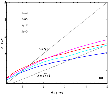
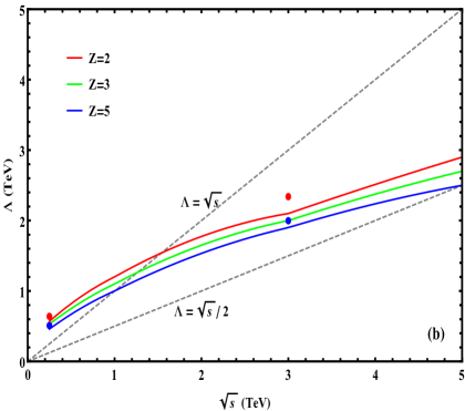
Figure 8: Reaches for the new physics scale $\Lambda$ as functions of the $e^{+}e^{-}$ collision energy $\sqrt{s\,}$ with an integrated luminosity $\,\mathcal{L}=2\text{ab}^{-1}$.  Plot (a) shows the $\Lambda$ reaches for the signal significances $(\mathcal{Z}_{4},\,\mathcal{Z}_{8})$ at $2\sigma$ and $5\sigma$ levels, respectively. Plot (b) depicts the combined sensitivity $\,\mathcal{Z}=\sqrt{\mathcal{Z}_{4}^{2}\!+\!\mathcal{Z}_{8}^{2}\,}=(2,\,3,\,5)\sigma$,  as shown by the (red, green, blue) curves. In this plot, the (red, blue) dots show the $(2\sigma,\,5\sigma)$ reaches with a projected integrated luminosity $\,\mathcal{L}=5\text{ab}^{-1}$ at $\sqrt{s\,}=\mathrm{250GeV}$ (CEPC and FCC-ee) and $\sqrt{s\,}=\mathrm{3TeV}$ (CLIC). For reference, we also show the lines $\,\Lambda=\!\sqrt{s\,}$  and $\,\Lambda=\!\sqrt{s\,}/2$  in each plot.

Finally, we present in Fig. 8 reaches for the new physics scale $\Lambda$ as functions of the $e^{+}e^{-}$ collision energy $\sqrt{s\,}$,  with a universal integrated luminosity $\,\mathcal{L}=2\,\text{ab}^{-1}$.  In Fig. 8(a), we show the $\Lambda$ reaches for the signal significances $(\mathcal{Z}_{4},\,\mathcal{Z}_{8})$ at $2\sigma$ and $5\sigma$ levels, respectively. Then, in Fig. 8(b), we depict the combined sensitivity $\,\mathcal{Z}\!=\!\sqrt{\mathcal{Z}_{4}\!+\!\mathcal{Z}_{8}\,}\!=(2,\,3,\,5)\sigma$ ,  shown as the (red, green, blue) curves. Furthermore, we present the sensitivity reaches with a projected integrated luminosity $\,\mathcal{L}=5\,\text{ab}^{-1}$ at $\sqrt{s\,}=\mathrm{250\,GeV}$ (CEPC and FCC-ee) and $\sqrt{s\,}=\mathrm{3\,TeV}$ (CLIC), shown as (red, blue) dots at $(2\sigma,\,5\sigma)$ level. For reference, we also show two lines $\,\Lambda\!=\!\sqrt{s\,}\,$ and $\,\Lambda\!=\!\sqrt{s\,}/2\,$ in each plot, since the effective field theory description may be expected to hold when $\,\Lambda\!>\!\sqrt{s\,}\,$ or $\,\Lambda\!>\!\sqrt{s\,}/2\,$.

We note that throughout the present study we have used $\Lambda$ to denote the cutoff scale, which is connected to another commonly used notation $\tilde{\Lambda}$ via $\,\tilde{\Lambda}\!=\!|c_{j}|^{1/4}\Lambda\,$,  as defined around Eq.(1). The cutoff $\tilde{\Lambda}$ may be regarded as the true new physics scale. The operators (2) invoke both gauge bosons and Higgs doublets. In a strongly-interacting underlying theory, the coefficient could be sizeable ($\,c_{j}\gg 1\,$), so the actual cutoff scale $\tilde{\Lambda}$ could be significantly larger than the quantity $\Lambda$ shown in Fig. 8. For instance, when $c_{j}\!\approx 4\pi$,  we have $\,\tilde{\Lambda}\approx 1.9\Lambda\,$.

In passing, it is clear that the same $ZZ\gamma$ nTGC contributes to both the processes $\,e^{+}e^{-}\!\!\rightarrow\!Z\gamma\,$ and $\,e^{+}e^{-}\!\!\rightarrow\!ZZ\,$, but the $Z\gamma$ final state is much simpler to analyze experimentally than $ZZ$, since the out-going photon can be detected directly and its energy and direction can be measured with good precision. Moreover, in this case the final state is a 3-body system after $Z$ decay, while the diboson $ZZ$ decays produce a more complicated 4-body final state. Besides, if one seeks to analyze leptonic $Z$-decays, each small leptonic $Z$-decay branching ratio Br$[Z\!\rightarrow\!\ell\bar{\ell}\,]\simeq 0.1$  reduces the signal by an order of magnitude, while hadronic $Z$-decays are harder to measure and disentangle. In the future, however, when a specific lepton collider and detector are eventually approved, it may be beneficial to study systematically all possible channels, including the $ZZ$ channel, for probing the nTGCs.

Before concluding this section, we make a final clarification. Since some dimension-6 operators contribute to the $Ze^{+}e^{-}$ vertex, they may cause possible deviations from the SM prediction for $e^{+}e^{-}\!\!\rightarrow\!Z\gamma$  via the $t$-channel exchange diagram. However, the $Ze^{+}e^{-}$ coupling has already been highly constrained by the current electroweak precision data, and will be much more severely constrained by $Z$-pole measurements at the future $e^{+}e^{-}$ colliders such as CEPC. For instance, Ref. GHX-2016 did a systematical study on the Higgs-related dimension-6 operators at $e^{+}e^{-}$ colliders, and derived the constraints from both the current data and the future $e^{+}e^{-}$ Higgs factory. We find that the following dimension-6 operators will contribute to the $Ze^{+}e^{-}$ vertex GHX-2016 ,

$$O^{(3)}_{L} \,=\, (\mathrm{i}H^{\dagger}\sigma^{a}\!\!\stackrel{{\scriptstyle\leftrightarrow}}{{D}}_{\mu}\!\!H)(\overline{\Psi}_{L}\gamma^{\mu}\sigma^{a}\Psi_{L})\,,$$ (54a)

$$\mathcal{O}_{L} \,=\, (\mathrm{i}H^{\dagger}\!\stackrel{{\scriptstyle\leftrightarrow}}{{D}}_{\mu}\!H)(\overline{\Psi}_{L}\gamma^{\mu}\Psi_{L})\,,$$ (54b)

$$\mathcal{O}_{R}\! \,=\, (\mathrm{i}H^{\dagger}\!\!\stackrel{{\scriptstyle\leftrightarrow}}{{D}}_{\mu}\!\!H)(\overline{\psi}_{R}\gamma^{\mu}\psi_{R})\,,$$ (54c)

where each operator is associated with the corresponding cutoff suppression factor $\,c_{j}/\tilde{\Lambda}^{2}\equiv\Lambda_{j}^{2}\,$.  From the analysis of Ref. GHX-2016 , we can extract the constraints from the current electroweak precision data, finding that cutoff scale of the dimension-6 operator $O^{(3)}_{L}$ is already bounded by $\,\Lambda>7.7\,$TeV ($2\sigma$ level). This is because $O^{(3)}_{L}$ contributes to both $Ze\bar{e}$ and $We\bar{\nu}$ vertices at the same time, and thus modifies $G_{F}$; while the other two operators $O_{L}$ and $O_{R}$ do not contribute to any of the precision observables among ($M_{Z}$, $M_{W}$, $G_{F}$, $\alpha_{\text{em}}$) GHX-2016 . After including the projected $Z$-pole measurements at the CEPC, we find that all the dimension-6 operators (54) will be severely constrained with their cutoff scales bounded by $\,\Lambda_{6}>21.2\!-\!34.5\,$TeV ($13.4\!-\!21.8\,$TeV) at the $2\sigma$ ($5\sigma$) level, as summarized in Table 4. On the other hand, our present nTGC study of the dimension-8 operator shows that the nTGC bounds obey $\,\Lambda_{8}\!>2.6$ TeV (2.1 TeV) at $2\sigma$ ($5\sigma$) level for collider energies up to $\sqrt{s}=3$ TeV (cf. Tables 6 and 7). Hence, the cutoff scale $\,\Lambda_{6}$ of the dimension-6 operators are already severely constrained to be substantially higher than our present nTGC bounds on the dimension-8 operator by about an order of magnitude, namely, $\,\Lambda_{6}=O(10)\Lambda_{8}\gg\Lambda_{8}\,$.

Dim-6 Operators	$\mathcal{O}_{L}^{(3)}$	$\mathcal{O}_{L}^{(3)}$	$\mathcal{O}_{L}$	$\mathcal{O}_{R}$
	(current bound)
$\Lambda_{2\sigma}$ (TeV)	7.7	34.5	19.2	21.2
$\Lambda_{5\sigma}$ (TeV)	4.8	21.8	12.2	13.4

Table 4: Constraints on the scales of dimension-6 operators (54) by the current electroweak precision data (2nd column) and by further including the $Z$-pole measurements at the CEPC (3rd–5th columns), at the $2\sigma$ level (2nd row) and the $5\sigma$ level (3rd row).

Using the relation $\,\Lambda_{6}=O(10)\Lambda_{8}$,  we can compare the contributions to $e^{-}e^{+}\!\!\rightarrow\!Z\gamma$ from a dimension-6 operator $\mathcal{O}_{6}$ in Eq.(54) and from the dimension-8 operator $\mathcal{O}_{8}\!=\!\mathcal{O}_{\widetilde{B}W}$.  We have presented in Appendix A.1 the contributions of the dimension-8 operator $\mathcal{O}_{8}$ to the helicity amplitudes for $ee\!\rightarrow\!Z\gamma$  as in Eq.(78); while for the current purpose of comparison, we can estimate the contributions of dimension-6 operators (54) by power-counting. With these, we summarize the estimated sizes of the contributions to the helicity amplitudes by both dimension-8 and dimension-6 operators,

$$\mathcal{T}_{(8)}[\pm\pm]\sim\frac{\,M_{Z}^{2}E^{2}\,}{\Lambda_{8}^{4}},~{}~{}~{}~{}~{}\mathcal{T}_{(8)}[\pm\mp]=0\,,~{}~{}~{}~{}~{}\mathcal{T}_{(8)}[0\pm]\sim\frac{\,M_{Z}E^{3}\,}{\Lambda_{8}^{4}},~{}~{}~{}~{}~{}$$ (55a)

$$\mathcal{T}_{(6)}[\pm\pm]\sim\frac{\,M_{Z}^{4}\,}{\,E^{2}\Lambda_{6}^{2}\,},~{}~{}~{}~{}~{}\mathcal{T}_{(6)}[\pm\mp]\sim\frac{M_{Z}^{2}}{\,\Lambda_{6}^{2}\,},~{}~{}~{}~{}\mathcal{T}_{(6)}[0\pm]\sim\frac{\,M_{Z}^{3}\,}{\,E\Lambda_{6}^{2}\,},$$ (55b)

where the helicity amplitude $\mathcal{T}_{(8)}[\pm\mp]$ vanishes due to the symmetry structure of $\mathcal{O}_{8}$.  For the $Z\gamma$ helicity combinations $\lambda\lambda^{\prime}=\pm\pm,\,0\pm$,  we find that the ratios of the $\mathcal{O}_{6}$ and $\mathcal{O}_{8}$ contributions are given by

$$\frac{\,\mathcal{T}_{(6)}\,}{\,\mathcal{T}_{(8)}\,}\sim\frac{M_{Z}^{2}}{\,E^{2}\,}\frac{\Lambda_{8}^{2}}{\,E^{2}\,}\frac{\,\Lambda_{8}^{2}\,}{\Lambda_{6}^{2}}\sim\frac{M_{Z}^{2}}{\,E^{2}\,}\frac{\,\Lambda_{8}^{2}\,}{\Lambda_{6}^{2}}\ll O(10^{-2})\,,$$ (56)

where $\,E\!=\!\!\sqrt{s}$  and $M_{Z}^{2}/E^{2}\!\ll\!1\,$.  For the nTGC analysis of $\mathcal{O}_{8}$, our Tables 6 and 7 show that the probed cutoff scale $\Lambda_{8}$ is close to or somewhat below the collider energy, $\Lambda_{8}\!\sim\!E$ ,  which is used in the second step of the above estimates. For the $Z\gamma$ helicity combinations $[\pm\mp]$ ,  the $\mathcal{O}_{8}$ contribution vanishes, and $\mathcal{T}_{(6)}[\pm\mp]$ just interferes with the SM amplitude $\mathcal{T}_{\text{sm}}[\pm\mp]$.  Thus, we can estimate this interference contribution to the cross section as $\,\sigma_{\!(6)}[\pm\mp]\sim\frac{M_{Z}^{2}}{\,E^{2}\Lambda^{2}_{6}\,}\,$. This will be compared to the interference contribution of $\mathcal{O}_{8}$ to the total cross section $\,\sigma_{\!(8)}\!\sim\!\frac{M_{Z}^{2}}{\Lambda_{8}^{4}}$  from Eq.(15), or, $\sigma_{8}(\mathbb{O}^{1}_{c})\sim\frac{EM_{Z}}{\Lambda_{8}^{4}}$ from Eq.(28a). With these, we estimate the following ratios:

$$\frac{\sigma_{\!(6)}[\pm\mp]}{\sigma_{\!(8)}}\sim\frac{\,\Lambda_{8}^{2}\,}{\Lambda_{6}^{2}}=O(10^{-2})\,,~{}~{}~{}~{}~{}\frac{\sigma_{\!(6)}[\pm\mp]}{\sigma_{\!(8)}(\mathbb{O}^{1}_{c})}\sim\frac{\,M_{Z}}{E}\frac{\,\Lambda_{8}^{2}\,}{\Lambda_{6}^{2}}<O(10^{-2})\,.\hskip 42.67912pt$$ (57)

The above analysis demonstrates that the contributions of such dimension-6 operators (54) are always negligible for energy scales $E\!\lesssim\!\Lambda_{8}$ ,  due to the severe independent constraints on their cutoff $\Lambda_{6}$ imposed by the current electroweak precision data and the projected future $Z$-pole measurements at CEPC, namely, $\,\Lambda_{6}=O(10)\Lambda_{8}\gg\Lambda_{8}\,$.  Moreover, we recall that these dimension-6 operators do not contribute to the nTGC and thus are irrelevant to our nTGC study. Hence, it is well justified to drop such dimension-6 operators (54) for the present nTGC study, which considers individually the relevant dimension-8 operator.

4 . Analysis of Invisible Decay Channels $Z\!\rightarrow\!\nu\bar{\nu}$

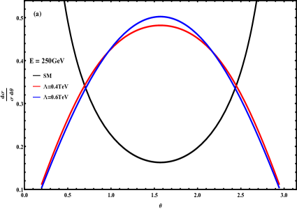
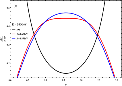
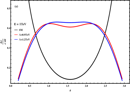
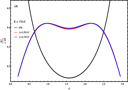
Figure 9: Normalized angular distributions for the scattering angle $\theta$ of the reaction $e^{-}e^{+}\!\!\rightarrow\!Z\gamma$ (with invisible decays $Z\!\!\rightarrow\!\nu\bar{\nu}$) in the lab frame and at different collision energies, $\sqrt{s}=(250\,\text{GeV},\,500\,\text{GeV},\,1\,\text{TeV},\,3\,\text{TeV})$. In each plot, the black curve denotes the SM contribution and the red and blue curves present the contributions from new physics with two sample values of $\,\Lambda$ .

In this section, we analyze $e^{-}e^{+}\!\!\!\rightarrow\!Z\gamma$ production followed by the invisible decays $Z\!\!\rightarrow\!\nu\bar{\nu}$ .  Then, we combine its sensitivity with that of the leptonic channels $Z\!\!\rightarrow\!\ell^{-}\ell^{+}$ presented in Section 3.

In the case of the invisible decay channels $Z\!\!\rightarrow\!\nu\bar{\nu}$,  we can apply the angular cut on the scattering angle of the final state mono-photon, $\,\delta_{m}\!\!<\!\theta\!<\pi\!-\delta_{m}$,  which corresponds to a cut on the photon transverse momentum $P^{\gamma}_{T}=q\sin\!\theta>q\sin\!\delta_{m}$.  The angular distributions of $\,\theta\,$ are presented in Fig. 9. We estimate the following optimal cuts $\,\delta_{m}\!\!<\!\theta\!<\pi\!-\delta_{m}$  with

$$\delta_{m}=\,(0.633,\,0.626,\,0.624,\,0.623,\,0.623),$$ (58)

for various collider energies $\sqrt{s\,}\!=(250,\,500,\,1000,\,3000,\,5000)$ GeV, respectively. We see that the optimal angular cut $\,\delta_{m}$  is not very sensitive to the variation of collider energy $\sqrt{s\,}$ .  The averaged value of the cuts (58) equals $\,\sin\!\delta_{m}\!\simeq 0.586$ ,  which restricts the scattering angle within the range

$$36^{\circ}\lesssim\,\theta\,\lesssim 144^{\circ}\,.$$ (59)

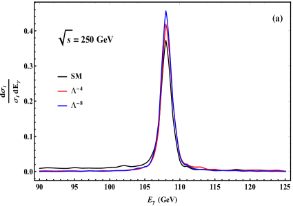
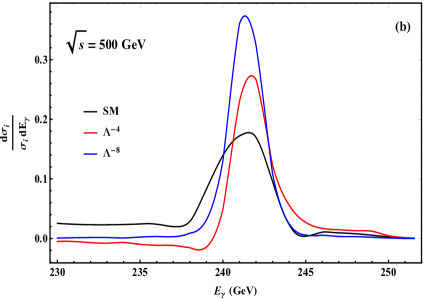
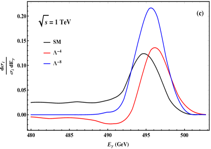
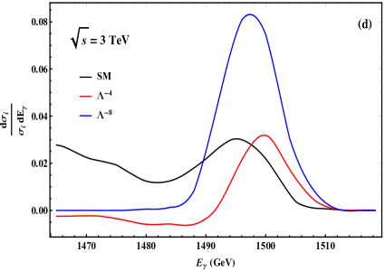
Figure 10: Normalized photon energy distributions for different collision energies, $\sqrt{s}=(250\,\text{GeV},\,500\,\text{GeV},\,1\,\text{TeV},\,3\,\text{TeV})$, where the experimental photon energy resolution (61) is included. In each plot, the (black, red, blue) curves present the SM contributions, the new physics contributions of $\,O(\Lambda^{-4})$ and $\,O(\Lambda^{-8})$, respectively.

Next, we study the photon energy distributions of the signals and backgrounds. According to the signal kinematics, the photon energy $\,E_{\gamma}\!=(s\!-\!M_{\nu\bar{\nu}}^{2})/(2\sqrt{s})$  and the invariant mass $\,M_{\nu\bar{\nu}}\!=M_{Z}$ .  To require $\nu\bar{\nu}$ mainly from on-shell $Z$-decays, we would normally set an invariant mass window, $\,M_{\nu\bar{\nu}}^{\pm}\!=M_{Z}\pm\delta$  with $\delta=10$ GeV. This corresponds to a variation in photon energy, $\,E_{\gamma}^{\pm}=(s-{M_{\nu\bar{\nu}}^{\mp}}^{2})/(2\sqrt{s})$,  with

$$\Delta E_{\gamma}=\,E_{\gamma}^{+}-E_{\gamma}^{-}=\frac{\,2M_{Z}\delta\,}{\,\sqrt{s\,}\,},$$ (60)

which is suppressed by  $2M_{Z}/\!\sqrt{s\,}$  and may be comparable to or smaller than the experimental energy resolution of photons in the detector for high energy $\,\sqrt{s}\gg 2M_{Z}$ .  As a result, one cannot impose a naive photon energy cut to ensure the on-shell decays $Z\!\!\rightarrow\!\nu\bar{\nu}$ via $\,E_{\gamma}^{-}<E_{\gamma}<E_{\gamma}^{+}$ .  To take into account the experimental photon-energy resolution, we may choose the current $E_{\gamma}$ resolution ($\sigma_{E}$) of the CMS detectors Sirunyan:2017ulk ; Chatrchyan:2013dga as a good estimate,

$$\frac{\,\sigma_{E}\,}{E}\,=\,\frac{2.8\%}{\,\sqrt{E/\textrm{GeV}\,}\,}\oplus\frac{12\%}{E/\textrm{GeV}\,}\oplus 0.3\%\,.$$ (61)

Thus, we set the photon energy cut as follows,

$$\min(E_{\gamma}^{-},\bar{E}_{\gamma}\!-\!2\sigma_{E})<E_{\gamma}<\max(E_{\gamma}^{+},\bar{E}_{\gamma}\!+\!2\sigma_{E})\,,$$ (62)

where $\,\bar{E}_{\gamma}=\,(s\!-\!M_{Z}^{2})/(2\sqrt{s})$ .  In our event simulations, $E_{\gamma}$ is the photon energy convoluted with the experimental resolution (61).

In Fig. 10, we present the normalized photon energy distributions for different collision energies $\sqrt{s\,}\!=(250\,\textrm{GeV},\,500\,\textrm{GeV},\,1\,\textrm{TeV},\,3\,\textrm{TeV})$. We find that the interference term of $O(\Lambda^{-4})$ is negligible for high collision energies $\sqrt{s}\gtrsim 3$ TeV; while for $\sqrt{s}\lesssim 1$ TeV, the interference term becomes important, in which the contribution of the SM $W$-exchange diagram [Fig. 7(e)] is negligible. We inspect the photon energy distributions at different collision energies in Fig. 10. We see that the SM background distribution (black color) and the new physics distribution (red color) have similar shapes for $\sqrt{s}\lesssim 500$ GeV, implying that the photon energy cut is not so useful here. This is because the SM $W$-exchange contribution [Fig. 7(e)] is negligible in such cases. But, for $\sqrt{s}\gtrsim\!1$ TeV, the shape of the new physics distribution differs from that of the SM backgrounds substantially, since the SM $W$-exchange contribution [Fig. 7(e)] becomes important. Hence, the photon energy cut becomes important for effectively suppressing the SM backgrounds, especially the SM $W$-exchange diagram in Fig. 7(e).

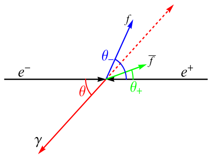
Figure 11: Illustration of kinematics of the reaction $\,e^{-}e^{+}\!\rightarrow f\bar{f}\gamma\,$, where the vector with red color denotes the photon 3-momentum $\vec{p}_{\gamma}$, and the vector with blue (green) color denotes the 3-momentum $\vec{p}_{f}$ ($\vec{p}_{\bar{f}}$) of the final state fermion $f$ ($\bar{f}$). The momentum conservation requires $(\vec{p}_{f}\!+\vec{p}_{\bar{f}})+\vec{p}_{\gamma}=0$ .  From this, we deduce: (i) either $\theta_{-}\!>\theta$  or $\,\theta_{+}\!>\theta$  for the case of $\,0^{\circ}\!<\!\theta\!<\!90^{\circ}$;  and (ii) either $\theta_{-}\!<\theta$ or $\,\theta_{+}\!<\theta$ for the case of $\,90^{\circ}\!<\!\theta\!<180^{\circ}$. 

Finally, in addition to the irreducible backgrounds for $e^{-}e^{+}\!\rightarrow\nu\bar{\nu}\gamma$ (Fig. 7), we have also considered the possible reducible background $e^{-}e^{+}\!\!\rightarrow\!e^{-}e^{+}\gamma$ with both $e^{-}$ and $e^{+}$ lost in the beam pipe. We illustrate the kinematics of this background process as in Fig. 11, the final state fermions $\,f\bar{f}=e^{-}e^{+}$.  As defined before (Fig. 1), the scattering angle $\theta$ is the angle between the moving directions of the incoming $e^{-}$ and outgoing $Z$, which equals the angle between the incoming $e^{+}$ and outgoing $\gamma$ (Fig. 11). For any final state $\,e^{-}e^{+}\gamma$ ,  the sum of the 3-momenta of $e^{-}$ and $e^{+}$ must cancel exactly the photon 3-momentum: $(\vec{p}_{e^{-}}\!+\vec{p}_{e^{+}}\!)+\vec{p}_{\gamma}=0$ .  In Fig. 11, we denote the angle between the moving directions of the final state $e^{-}$ ($e^{+}$) and initial state $e^{-}$ as $\theta_{-}$ ($\theta_{+}$). Thus, we must have: (i) either $\theta_{-}\!>\theta$  or  $\theta_{+}\!>\theta$  for the case of $\,0^{\circ}\!<\!\theta\!<\!90^{\circ}$;  and (ii) either $\theta_{-}\!<\theta$  or  $\theta_{+}\!<\theta$  for the case of $\,90^{\circ}\!<\!\theta\!<180^{\circ}$.  We observe that in both cases (i) and (ii) at least one of the final state $e^{-}$ and $e^{+}$ must have its moving direction deviate more from the beam pipe than the outgoing photon. Because we have imposed significant angular cuts (59) that restrict the scattering angle of the outgoing photon within the range $\,36^{\circ}\lesssim\theta\lesssim 144^{\circ}$,  we know that at least one of the outgoing $e^{-}$ and $e^{+}$ must have its angle ($\theta_{-}$ or $\theta_{+}$) fall into this window $\,36^{\circ}\lesssim\theta_{\mp}\lesssim 144^{\circ}$,  and thus cannot escape the detector. This shows that there is no chance that both the final-state particles $e^{-}$ and $e^{+}$ could escape detection, so such $e^{-}e^{+}\gamma$ events can be always vetoed. Therefore, under the cuts (59), the reducible $e^{-}e^{+}\gamma$ background is fully negligible in our study.

With the photon angular cut (58) and energy cut (62), we compute the cross section of $\,e^{-}e^{+}\!\!\rightarrow\nu\bar{\nu}\gamma$  as a function of the new physics scale $\Lambda$ ,

$$\sqrt{s\,}\!=250~{}\text{GeV}, \sigma(\nu\bar{\nu}\gamma)=\left[635\pm 1.33\!\left(\!\frac{\,0.5\text{TeV}\,}{\Lambda}\!\right)^{\!\!4}\!+0.282\!\left(\!\frac{\,0.5\text{TeV}\,}{\Lambda}\!\right)^{\!\!8}\right]\!\text{fb}\,,~{}~{}~{}~{}~{}~{}~{}~{}$$ (63a)

$$\sqrt{s\,}\!=500~{}\text{GeV}, \sigma(\nu\bar{\nu}\gamma)=\left[126\pm 0.201\!\left(\!\frac{\,0.8\text{TeV}\,}{\Lambda}\!\right)^{\!\!4}\!+0.124\!\left(\!\frac{\,0.8\text{TeV}\,}{\Lambda}\!\right)^{\!\!8}\right]\!\text{fb}\,,$$ (63b)

$$\sqrt{s\,}\!=1~{}\text{TeV}, \sigma(\nu\bar{\nu}\gamma)=\left[33.8\pm 0.086\!\left(\!\frac{\,\text{TeV}\,}{\Lambda}\!\right)^{\!\!4}+0.370\!\left(\!\frac{\,\text{TeV}\,}{\Lambda}\!\right)^{\!\!8}\right]\!\text{fb}\,,$$ (63c)

$$\sqrt{s\,}\!=3~{}\text{TeV}, \sigma(\nu\bar{\nu}\gamma)=\left[4.28\pm 0.004\!\left(\!\frac{\,2\text{TeV}\,}{\Lambda}\!\right)^{\!\!4}+0.124\!\left(\!\frac{\,2\text{TeV}\,}{\Lambda}\!\right)^{\!\!8}\right]\!\text{fb}\,,$$ (63d)

$$\sqrt{s\,}\!=5~{}\text{TeV}, \sigma(\nu\bar{\nu}\gamma)=\left[1.78\pm 0.001\!\left(\!\frac{\,2.5\text{TeV}\,}{\Lambda}\!\right)^{\!\!4}+0.160\!\left(\!\frac{\,2.5\text{TeV}\,}{\Lambda}\!\right)^{\!\!8}\right]\!\text{fb}\,.\hskip 42.67912pt$$ (63e)

With these, we derive the signal significance $\mathcal{Z}_{8}$ as follows:

$$\sqrt{s}=250\,\text{GeV}, \mathcal{Z}_{8,\nu\bar{\nu}}=\left|\pm 2.36\!\left(\!\frac{\,0.5\text{TeV}\,}{\Lambda}\!\right)^{\!\!4}\!+0.501\!\left(\!\frac{\,0.5\text{TeV}\,}{\Lambda}\!\right)^{\!\!8}\right|\!\times\!\sqrt{\epsilon\,}\,,\hskip 71.13188pt$$ (64a)

$$\sqrt{s}=500\,\text{GeV}, \mathcal{Z}_{8,\nu\bar{\nu}}=\left|\pm 0.801\left(\!\frac{\,0.8\text{TeV}\,}{\Lambda}\!\right)^{\!\!4}\!+0.493\!\left(\!\frac{\,0.8\text{TeV}\,}{\Lambda}\!\right)^{\!\!8}\right|\!\times\!\sqrt{\epsilon\,}\,,$$ (64b)

$$\sqrt{s}=1\,\text{TeV}, \mathcal{Z}_{8,\nu\bar{\nu}}=\left|\pm 0.650\!\left(\!\frac{\,\text{TeV}\,}{\Lambda}\!\right)^{\!\!4}\!+2.85\!\left(\!\frac{\,\text{TeV}\,}{\Lambda}\!\right)^{\!\!8}\right|\!\times\!\sqrt{\epsilon\,}\,,$$ (64c)

$$\sqrt{s}=3\,\text{TeV}, \mathcal{Z}_{8,\nu\bar{\nu}}=\left|\pm 0.09\!\left(\!\frac{\,2\,\text{TeV}\,}{\Lambda}\!\right)^{\!\!4}\!+2.69\!\left(\!\frac{\,2\,\text{TeV}\,}{\Lambda}\!\right)^{\!\!8}\right|\!\times\!\sqrt{\epsilon\,}\,,$$ (64d)

$$\sqrt{s}=5\,\text{TeV}, \mathcal{Z}_{8,\nu\bar{\nu}}=\left|\pm 0.04\!\left(\!\frac{\,2.5\text{TeV}\,}{\Lambda}\!\right)^{\!\!4}\!+5.38\!\left(\!\frac{\,2.5\text{TeV}\,}{\Lambda}\!\right)^{\!\!8}\right|\!\times\!\sqrt{\epsilon\,}\,.$$ (64e)

$\sqrt{s\,}$ (GeV)	250	500	1000	3000	5000
$\Lambda$ (TeV)	0.5	0.7	1.0	1.9	2.6
$\mathcal{Z}_{\ell\bar{\ell}}$	3.6(3.2)	4.1(3.4)	4.5(3.9)	4.4(4.2)	4.2(4.1)
$\mathcal{Z}_{8,\nu\bar{\nu}}$	2.9(2.3)	2.8(0.07)	3.4(2.2)	4.1(3.9)	4.0(3.9)
$\mathcal{Z}$(combined)	4.6(3.9)	5.0(3.4)	5.6(4.5)	6.0(5.8)	5.8(5.6)

Table 5: Signal significances for the dilepton channels (3rd row) and invisible channels (4th row) at different collider energies (shown in the 1st row). For each collider energy $\sqrt{s\,}$, we assume a representative new physics scale $\Lambda$ (shown in the 2nd row). The combined signal significance $\mathcal{Z}$(combined) for each collision energy is presented in the last row. Here the numbers in the parentheses correspond to the case of the dimension-8 operator whose coefficient is negative. For illustration, we have assumed a fixed representative integrated luminosity $\,\mathcal{L}=2\,\text{ab}^{-1}\!$ and an ideal detection efficiency $\,\epsilon=100\%$.

In Table 5, we present the signal significances at different collider energies (shown in the first row), for the dilepton channels $Z\!\!\rightarrow\!\ell^{-}\ell^{+}$ (third row) and for the invisible channels $Z\!\!\rightarrow\!\nu\bar{\nu}$ (fourth row). For each collider energy $\sqrt{s\,}$, we input the relevant sample new physics scale $\Lambda$ ,  as shown in the second row. We see that the signal significances of these two types of channels are comparable, with the dilepton channels being more sensitive for $\sqrt{s\,}\lesssim 2.5$ TeV, whereas their sensitivities become fairly close for $\sqrt{s\,}\gtrsim 3$ TeV. We present the combined signal significance $\,\mathcal{Z}(\text{combined})\!=\!\sqrt{\!\mathcal{Z}_{\ell\bar{\ell}}^{2}+\!\mathcal{Z}_{8,\nu\bar{\nu}}^{2}}$ ,  in the last row for each given collision energy. This shows that in each case the combined sensitivity is enhanced over the individual channels by a sizeable factor of about $1.2-\!1.4$.  As previously, the numbers in the parentheses of Table 5 correspond to the case of the dimension-8 operator with a negative coefficient. For illustration, we have assumed a fixed representative integrated luminosity $\,\mathcal{L}\!=\!2\,\text{ab}^{-1}\!$ and an ideal detection efficiency $\,\epsilon=100\%$ .

By requiring $\mathcal{Z}_{8}\!=2$ and $\mathcal{Z}_{8}\!=5$  in Eq.(64), we derive the reaches for the new physics scale $\,\Lambda\,$ at the $2\sigma$ and $5\sigma$ levels, denoted as $\Lambda^{2\sigma}_{\nu\bar{\nu}}$ and $\Lambda^{5\sigma}_{\nu\bar{\nu}}$ ,  respectively. We summarize the findings in Table 6, as shown in the fourth and fifth rows. For comparison, we also list the new physics reaches $\Lambda^{2\sigma}_{\ell\bar{\ell}}$ and $\Lambda^{5\sigma}_{\ell\bar{\ell}}$ (second and third rows of Table 6) from the dilepton channels of Table 3. Then, we derive the combined sensitivity reaches of the new physics scale $\Lambda$ from both the dilepton channels and invisible channels, which are presented in the sixth and seventh rows of the current Table 6, denoted as $\Lambda^{2\sigma}_{\ell\nu,\text{comb}}$ and $\Lambda^{5\sigma}_{\ell\nu,\text{comb}}$. We see that the combined bounds $\Lambda^{2\sigma}_{\ell\nu,\text{comb}}$ and $\Lambda^{5\sigma}_{\ell\nu,\text{comb}}$ are only slightly enhanced compared to the analysis using the $Z\!\!\rightarrow\!\ell^{+}\ell^{-}$  channel alone. This can be understood by noting that the new physics scale $\Lambda$ is rather insensitive to the significance $\mathcal{Z}$,  because Eqs.(40) and (44) show, $\Lambda\!\propto\!\mathcal{Z}_{4}^{-\frac{1}{4}}$ (when the $\Lambda^{\!-4}$ contribution dominates the signal) and $\Lambda\!\propto\!\mathcal{Z}_{8}^{-\frac{1}{8}}$ (when the $\Lambda^{\!-8}$ contribution dominates the signal).

$\sqrt{s\,}$ (GeV)	250	500	1000	3000	5000
$\Lambda^{2\sigma}_{\ell\bar{\ell}}$ (TeV)	0.57(0.56)	0.82(0.80)	1.2	2.1	2.9
$\Lambda^{5\sigma}_{\ell\bar{\ell}}$ (TeV)	0.46(0.44)	0.67(0.64)	0.98(0.95)	1.9	2.5
$\Lambda^{2\sigma}_{\nu\bar{\nu}}$ (TeV)	0.54(0.32)	0.74(0.61)	1.1(1.0)	2.1	2.8
$\Lambda^{5\sigma}_{\nu\bar{\nu}}$ (TeV)	0.44(0.32)	0.64(0.56)	0.96(0.91)	1.9(1.8)	2.5
$\Lambda^{2\sigma}_{\ell\nu,\text{comb}}$ (TeV)	0.61(0.59)	0.85(0.80)	1.2	2.2	3.0
$\Lambda^{5\sigma}_{\ell\nu,\text{comb}}$ (TeV)	0.49(0.46)	0.70(0.64)	1.0(0.91)	2.0(1.9)	2.6

Table 6: Sensitivity reaches for the new physics scale $\Lambda$ from the $\,e^{-}e^{+}\!\!\rightarrow\!\nu\bar{\nu}\gamma$  channel, and from combining both $\ell^{-}\ell^{+}\gamma$ and $\nu\bar{\nu}\gamma$ channels, at the $2\sigma$ and $5\sigma$ levels, for different collider energies. Here again the numbers in parentheses correspond to the case of the dimension-8 operator whose coefficient has a minus sign, while in all other entries the differences between the two signs of the coefficient are negligible. For illustration, we have assumed a fixed representative integrated luminosity $\,\mathcal{L}=2\,\text{ab}^{-1}\!$ and an ideal detection efficiency $\,\epsilon=100\%$ .

5 . Improvements from $\boldsymbol{e^{\mp}}$ Beam Polarizations

In this section, we extend our analysis to include the effects of initial-state electron/positron polarizations, and demonstrate how the sensitivity reaches of new physics scale $\Lambda$ can be improved.

Using the helicity amplitude (A.2), we derive the leading contribution to the differential cross section at $\mathcal{O}(\Lambda^{\!-4})$,  which is proportional to the interference term,

$$\Re\texttt{e}\!\!\left[\mathcal{T}^{L}_{(8)}(0\pm)\mathcal{T}^{T*}_{\text{sm}}(\mp\pm)\right]\!\sin\theta\sin\theta_{*}$$ (65)

$$\propto\displaystyle\frac{v^{2}\!\sqrt{s\,}}{\,\Lambda^{4}M_{Z}\,}\!\!\left[({e_{L}^{2}}\!+\!{e_{R}^{2}})(f_{L}^{2}\!-\!f_{R}^{2})(1\!+\!\cos^{2}\theta)+2({e_{L}^{2}}\!-\!{e_{R}^{2}})(f_{L}^{2}\!+\!f_{R}^{2})\cos\!\theta\cos\!\theta_{*}\right]\sin^{2}\!\theta_{*}\cos\phi_{*},~{}~{}~{}$$

where $\,(e_{L},\,e_{R})=(c_{L}\delta_{\!s,-\frac{1}{2}},\,c_{R}\delta_{\!s,\frac{1}{2}})$  are the $Z$ gauge couplings to the (left, right)-handed electrons, with the index $\,s=\mp\mbox{$\frac{\,{1}\,}{2}$}$  denoting the initial-state electron helicities. The final-state $Z$ boson decays into leptons $\ell^{-}\ell^{+}$ with couplings $\,(f_{L},\,f_{R})=(c_{L}\delta_{\!\sigma,-\frac{1}{2}},\,c_{R}\delta_{\!\sigma,\frac{1}{2}})$,  where $\sigma$ denotes the helicity of the massless lepton $\ell^{-}$ and  $(c_{L},\,c_{R})=(s_{W}^{2}\!-\!\mbox{$\frac{\,{1}\,}{2}$},\,s_{W}^{2})$  give the $Z$ gauge couplings to the (left, right)-handed leptons. We note from the right-hand-side (RHS) of Eq.(65) that for unpolarized initial states $e^{\mp}$ the observable $\mathbb{O}^{1}_{c}$ is suppressed by the coupling factor $\,f_{L}^{2}\!-\!f_{R}^{2}\propto\frac{1}{4}\!-\!\sin^{2}\!\theta_{W}$  in the first term, and the second term is suppressed by the coupling factor $\,e_{L}^{2}\!-\!e_{R}^{2}$ plus the factors $\cos\!\theta\cos\!\theta_{*}$ which can be either positive or negative. If the initial-state $e^{\mp}$ are polarized, we can largely remove the suppressions in the second term of the RHS of Eq.(65), since the coupling factor $\,e_{L}^{2}\!-\!e_{R}^{2}$ is replaced by $e_{L}^{2}$ (or $e_{R}^{2}$) in the fully-polarized case, and the factors $\cos\!\theta\cos\!\theta_{*}$ can be made positive by defining $\mathbb{O}^{1}_{c}$ appropriately.

In the ideal case of a fully left-polarized $e^{-}$ beam, we can redefine $\mathbb{O}^{1}_{c}$ as follows:

$$\mathbb{O}^{1}_{c} = \left|\sigma_{1}\!\int\!\!\mathrm{d}\theta\mathrm{d}\theta_{*}\mathrm{d}\phi_{*}\mathrm{d}M_{*}\,f^{1}\text{sign}(\cos\theta)\,\text{sign}(\cos\theta_{*})\,\text{sign}(\cos\phi_{*})\right|,\hskip 34.1433pt$$ (66a)

$$f_{j} = \displaystyle\frac{\mathrm{d}^{4}\sigma_{j}}{\,\sigma_{j}\mathrm{d}\theta\,\mathrm{d}\theta_{*}\mathrm{d}\phi_{*}\mathrm{d}M_{*}\,}\,,$$ (66b)

where $\,M_{*}\,$ is the invariant-mass of the final state leptons $\ell^{-}\ell^{+}$.  As can be readily seen, in this case the first term on the RHS of Eq.(65) gives zero contribution to the observable $\,\mathbb{O}^{1}_{c}$ .  Thus, $\,\mathbb{O}^{1}_{c}$  is dominated by the leading contributions of the second term on the RHS of Eq.(65), and is proportional to $\,c_{L}^{2}(c_{L}^{2}\!+\!c_{R}^{2})$  rather than $\,(c_{L}^{2}\!-\!c_{R}^{2})(c_{L}^{2}\!+\!c_{R}^{2})$ . Thus, at different collider energies, we can derive the following signal significance $\mathcal{Z}_{4}$ for the final state $e^{-}e^{+}\gamma$ ,

$$\sqrt{s}=250\,\text{GeV}, \mathcal{Z}_{4}^{e}=\,4.46\!\left(\!\frac{\,0.5\text{TeV}\,}{\Lambda}\!\right)^{\!\!\!4}\!\times\!\sqrt{\epsilon\,}\,,\hskip 34.1433pt$$ (67a)

$$\sqrt{s}=500\,\text{GeV}, \mathcal{Z}_{4}^{e}=\,3.64\!\left(\!\frac{\,0.8\text{TeV}\,}{\Lambda}\!\right)^{\!\!\!4}\!\times\!\sqrt{\epsilon\,}\,,$$ (67b)

$$\sqrt{s}=1\,\text{TeV}, \mathcal{Z}_{4}^{e}=\,6.40\!\left(\!\frac{\,\text{TeV}\,}{\Lambda}\!\right)^{\!\!\!4}\!\times\!\sqrt{\epsilon\,}\,,$$ (67c)

$$\sqrt{s}=3\,\text{TeV}, \mathcal{Z}_{4}^{e}\,=\,3.80\!\left(\!\frac{\,2\text{TeV}\,}{\Lambda}\!\right)^{\!\!\!4}\!\times\!\sqrt{\epsilon\,}\,,$$ (67d)

$$\sqrt{s}=5\,\text{TeV}, \mathcal{Z}_{4}^{e}=\,4.32\!\left(\!\frac{\,2.5\text{TeV}\,}{\Lambda}\!\right)^{\!\!\!4}\!\times\!\sqrt{\epsilon\,}\,;$$ (67e)

for the final state $\mu^{-}\mu^{+}\gamma$ ,

$$\sqrt{s}=250\,\text{GeV}, \mathcal{Z}_{4}^{\mu}=\,4.86\!\left(\!\frac{\,0.5\text{TeV}\,}{\Lambda}\!\right)^{\!\!\!4}\!\times\!\sqrt{\epsilon\,}\,,\hskip 34.1433pt$$ (68a)

$$\sqrt{s}=500\,\text{GeV}, \mathcal{Z}_{4}^{\mu}=\,3.78\!\left(\!\frac{\,0.8\text{TeV}\,}{\Lambda}\!\right)^{\!\!\!4}\!\times\!\sqrt{\epsilon\,}\,,$$ (68b)

$$\sqrt{s}=1\,\text{TeV}, \mathcal{Z}_{4}^{\mu}=\,6.47\!\left(\!\frac{\,\text{TeV}\,}{\Lambda}\!\right)^{\!\!\!4}\!\times\!\sqrt{\epsilon\,}\,,$$ (68c)

$$\sqrt{s}=3\,\text{TeV}, \mathcal{Z}_{4}^{\mu}\,=\,3.80\!\left(\!\frac{\,2\text{TeV}\,}{\Lambda}\!\right)^{\!\!\!4}\!\times\!\sqrt{\epsilon\,}\,,$$ (68d)

$$\sqrt{s}=5\,\text{TeV}, \mathcal{Z}_{4}^{\mu}=\,4.33\!\left(\!\frac{\,2.5\text{TeV}\,}{\Lambda}\!\right)^{\!\!\!4}\!\times\!\sqrt{\epsilon\,}\,;$$ (68e)

and for the $\tau^{-}\tau^{+}\gamma$ final state we have $\,\mathcal{Z}_{4}^{\tau}\simeq\mathcal{Z}_{4}^{\mu}$.

In reality, the $e^{\mp}$ beams could only be partially polarized. Let $P_{L}^{e}$ ($P_{R}^{\bar{e}})$ denote the left (right) polarization of the electrons (positrons) in the beam. We then have the following relations between the observable $\mathbb{O}^{1}_{c}$ with partial and full polarizations:

$$\mathbb{O}^{1}_{c}(P_{L}^{e},P_{R}^{\bar{e}}) \simeq \left|\frac{\,c_{L}^{2}P_{L}^{e}P_{R}^{\bar{e}}\!-\!c_{R}^{2}(\!1\!-\!P_{L}^{e})(\!1\!-\!P_{R}^{\bar{e}})\,}{c_{L}^{2}}\right|\mathbb{O}^{1}_{c}(1,1)\,,$$ (69a)

$$\sigma^{0}_{c}(P_{L}^{e},P_{R}^{\bar{e}}) \simeq \frac{\,c_{L}^{2}P_{L}^{e}P_{R}^{\bar{e}}\!+\!c_{R}^{2}(\!1\!-\!P_{L}^{e})(\!1\!-\!P_{R}^{\bar{e}})\,}{c_{L}^{2}}\sigma^{0}_{c}(1,1)\,,$$ (69b)

$$\mathcal{Z}_{4}(P_{L}^{e},P_{R}^{\bar{e}}) \simeq \frac{\,\left|c_{L}^{2}P_{L}^{e}P_{R}^{\bar{e}}\!-\!c_{R}^{2}(\!1\!-\!P_{L}^{e})(\!1\!-\!P_{R}^{\bar{e}})\right|\,}{\,|c_{L}|\sqrt{c_{L}^{2}P_{L}^{e}P_{R}^{\bar{e}}\!+\!c_{R}^{2}(\!1\!-\!P_{L}^{e})(1\!-\!P_{R}^{\bar{e}})}\,}\mathcal{Z}_{4}(1,1)\,,$$ (69c)

where the signal significance of the fully polarized case, $\,\mathcal{Z}_{4}(1,1)\!=\!\sqrt{(\mathcal{Z}_{4}^{e})^{2}\!+\!(\mathcal{Z}_{4}^{\mu})^{2}\!+\!(\mathcal{Z}_{4}^{\tau})^{2}}$,  with $(\mathcal{Z}_{4}^{e},\mathcal{Z}_{4}^{\mu},\mathcal{Z}_{4}^{\tau})$ given by Eqs.(67)-(68). For instance, assuming the polarizations $(P_{L}^{e},\,P_{R}^{\bar{e}})=(0.9,\,0.65)$, we derive

$$\mathcal{Z}_{4}(P_{L}^{e},P_{R}^{\bar{e}})\,\simeq\,0.715\;\mathcal{Z}_{4}(1,1)\,.$$ (70)

We note that the $e^{\mp}$ polarization possibilities have been well studied for the linear colliders ILC ILC and CLIC CLIC , whereas the longitudinal polarization is harder to realize at the circular colliders CEPC CEPC and FCC-$ee$ FCCee .

We can derive the following relations between the the cross sections $(\sigma_{0},\,\sigma_{1},\,\sigma_{2})$ for the partially polarized and unpolarized cases:

$$\sigma_{0}(P_{L}^{e},P_{R}^{\bar{e}}) = \frac{\,c_{L}^{2}P_{L}^{e}P_{R}^{\bar{e}}\!+\!c_{R}^{2}(\!1\!-\!P_{L}^{e})(\!1\!-\!P_{R}^{\bar{e}})}{\,0.5^{2}(c_{L}^{2}\!+\!c_{R}^{2})\,}\sigma_{0}(0.5,0.5)\,,$$ (71a)

$$\sigma_{1}(P_{L}^{e},P_{R}^{\bar{e}}) = \frac{\,c_{L}^{2}P_{L}^{e}P_{R}^{\bar{e}}\!-\!c_{R}^{2}(\!1\!-\!P_{L}^{e})(\!1\!-\!P_{R}^{\bar{e}})}{\,0.5^{2}(c_{L}^{2}\!-\!c_{R}^{2})\,}\sigma_{1}(0.5,0.5)\,,$$ (71b)

$$\sigma_{2}(P_{L}^{e},P_{R}^{\bar{e}}) = \frac{\,c_{L}^{2}P_{L}^{e}P_{R}^{\bar{e}}\!+\!c_{R}^{2}(\!1\!-\!P_{L}^{e})(\!1\!-\!P_{R}^{\bar{e}})}{\,0.5^{2}(c_{L}^{2}\!+\!c_{R}^{2})\,}\sigma_{2}(0.5,0.5)\,,$$ (71c)

where $\,(P_{L}^{e},\,P_{R}^{\bar{e}})\!=\!(0.5,\,0.5)$  corresponds to the unpolarized case.

$\sqrt{s\,}$ (GeV)	250	500	1000	3000	5000
$\Lambda^{2\sigma}_{\ell\bar{\ell}}$ (TeV)	0.81	1.1	1.5(1.4)	2.5	3.2
$\Lambda^{5\sigma}_{\ell\bar{\ell}}$ (TeV)	0.64	0.87(0.85)	1.2(1.1)	2.1(2.0)	2.7
$\Lambda^{2\sigma}_{\nu\bar{\nu}}$ (TeV)	0.85	1.0	1.3(0.86)	2.1	2.9(2.8)
$\Lambda^{5\sigma}_{\nu\bar{\nu}}$ (TeV)	0.67	0.84(0.80)	1.1(0.82)	1.9	2.6(2.5)
$\Lambda^{2\sigma}_{\ell\nu,\text{Comb}}$ (TeV)	0.90	1.2(1.0)	1.5	2.6(2.5)	3.3
$\Lambda^{5\sigma}_{\ell\nu,\text{Comb}}$ (TeV)	0.72	0.93(0.91)	1.2	2.1(2.0)	2.8(2.7)

Table 7: Sensitivity reaches of the new physics scale $\Lambda$ via $\,e^{-}e^{+}\!\!\rightarrow\!\ell^{-}{\ell}^{+}\gamma$  and $\,e^{-}e^{+}\!\!\rightarrow\!\nu\bar{\nu}\gamma$  channels and their combinations, for polarized $e^{\mp}$ beams with $(P_{L}^{e},\,P_{R}^{\bar{e}})=(0.9,\,0.65)$.  The bounds are shown at the $2\sigma$ and $5\sigma$ levels, and for different collider energies. As previously, the numbers in parentheses correspond to the case of the dimension-8 operator with negative coefficient, while in all other entries the effects of the sign of the coefficient are negligible. For illustration, we assume a representative integrated luminosity $\,\mathcal{L}=2\,\text{ab}^{-1}\!$ and an ideal detection efficiency $\,\epsilon=100\%$.

For the signal significance $\mathcal{Z}_{8}$, we denote its $\mathcal{O}(\Lambda^{-4})$ contribution as $\mathcal{Z}_{8}^{(4)}$ and its $\mathcal{O}(\Lambda^{-8})$ contribution as $\mathcal{Z}_{8}^{(8)}$,  with $\mathcal{Z}_{8}=\mathcal{Z}_{8}^{(4)}\!\!+\!\mathcal{Z}_{8}^{(8)}$.  We obtain the following signal significances $\mathcal{Z}_{8}$ with partial polarizations $(P_{L}^{e},P_{R}^{\bar{e}})$:

$$\mathcal{Z}_{8}(P_{L}^{e},P_{R}^{\bar{e}}) = \mathcal{Z}_{8}^{(4)}\!(P_{L}^{e},P_{R}^{\bar{e}})+\mathcal{Z}_{8}^{(8)}\!(P_{L}^{e},P_{R}^{\bar{e}}),$$ (72a)

$$\mathcal{Z}_{8}^{(4)}\!(P_{L}^{e},P_{R}^{\bar{e}}) = \frac{\,2\!\sqrt{c_{L}^{2}\!+\!c_{R}^{2}}\,}{\,c_{L}^{2}\!-\!c_{R}^{2}\,}\frac{\,c_{L}^{2}P_{L}^{e}P_{R}^{\bar{e}}\!-\!c_{R}^{2}(\!1\!-\!P_{L}^{e})(\!1\!-\!P_{R}^{\bar{e}})\,}{\,\sqrt{c_{L}^{2}P_{L}^{e}P_{R}^{\bar{e}}\!+\!c_{R}^{2}(\!1\!-\!P_{L}^{e})(\!1\!-\!P_{R}^{\bar{e}})}\,}\mathcal{Z}_{8}^{(4)}\!(0.5,0.5),\hskip 45.5244pt$$ (72b)

$$\mathcal{Z}_{8}^{(8)}\!(P_{L}^{e},P_{R}^{\bar{e}}) = 2\sqrt{\frac{c_{L}^{2}P_{L}^{e}P_{R}^{\bar{e}}\!+\!c_{R}^{2}(\!1\!-\!P_{L}^{e})(\!1\!-\!P_{R}^{\bar{e}})}{c_{L}^{2}\!+\!c_{R}^{2}}}\mathcal{Z}_{8}^{(8)}\!(0.5,0.5).$$ (72c)

For instance, with $e^{\mp}$ beam polarizations $(P_{L}^{e},\,P_{R}^{\bar{e}})=(0.9,\,0.65)$,  we find the following relation,

$$\mathcal{Z}_{8}(P_{L}^{e},P_{R}^{\bar{e}})\,\simeq\,7.18\mathcal{Z}_{8}^{(4)}\!(0.5,0.5)+1.19\mathcal{Z}_{8}^{(8)}\!(0.5,0.5)\,,$$ (73)

where the contributions $\mathcal{Z}_{8}^{(4)}\!(0.5,0.5)$ and $\mathcal{Z}_{8}^{(8)}\!(0.5,0.5)$ correspond to the unpolarized case, as computed in Section 3-4.

From Eqs.(70)(67)(68) and Eqs.(73), we compute the sensitivity reaches of the new physics scale $\Lambda$ via $\,e^{-}e^{+}\!\!\rightarrow\!\ell^{-}{\ell}^{+}\gamma$  and $\,e^{-}e^{+}\!\!\rightarrow\!\nu\bar{\nu}\gamma$  channels, for polarized electron/positron beams with $(P_{L}^{e},\,P_{R}^{\bar{e}})=(0.9,\,0.65)$.  These results are summarized in Table 7. Here the numbers in the parentheses correspond to the case of the dimension-8 operator with negative coefficient, while in all other entries the differences for opposite signs of the coefficient are negligible. For illustration, we have assumed a representative integrated luminosity $\,\mathcal{L}=2\,\text{ab}^{-1}\!$ and an ideal detection efficiency $\,\epsilon=100\%$ .

We present in Table 7 the $2\sigma$ and $5\sigma$ bounds on $\Lambda$ for different collider energies. The limits from the $\,\ell^{-}{\ell}^{+}\gamma$  channel are shown in the 2nd and 3rd rows, while the 4th and 5th rows give the limits in the $\nu\bar{\nu}\gamma$ channel. Finally, we derive the combined limits of $\,\ell^{-}{\ell}^{+}\gamma$ and $\nu\bar{\nu}\gamma$ channels, as shown in the 6th and 7th rows. Comparing the results in Table 7 with those in the previous Table 6, we see that for collider energies $\sqrt{s}=(250\!-\!1000)$ GeV, the $e^{\mp}$ beam polarizations can enhance the sensitivity reaches of $\Lambda$ significantly, by about $(47\!-\!25)\%$ [$(47\!-20\!)\%$] for the $2\sigma$ [$5\sigma$] limits; whereas for $\sqrt{s}=(3\!-\!5)$ TeV, the polarization effects are much milder, yielding an enhancement around $(18\!-\!10)\%$ [$(5\!-\!8)\%$] for the $2\sigma$ [$5\sigma$] limits. This feature is expected because the polarized $e^{\mp}$ beams help to remove the large cancellation in the coupling factor $\,c_{L}^{2}\!-c_{R}^{2}\!\propto\!\frac{1}{4}\!-\sin^{2}\!\theta_{W}$ of the $O(\Lambda^{-4})$ interference cross section (15) [or the coupling factor $\,e_{L}^{2}\!-e_{R}^{2}=c_{L}^{2}\!-c_{R}^{2}\,$ in Eq.(65)], and thus will mainly enhance the sensitivity $\mathcal{Z}_{4}$ . But, the polarized $e^{\mp}$ have rather minor effect on the $O(\Lambda^{-8})$ cross section because the coupling factor $\,c_{L}^{2}\!+c_{R}^{2}$  in Eq.(15) has no special cancellation. This is clear from Eqs.(73) and (72) which show that adding the $e^{\mp}$ polarizations enhances the $\mathcal{Z}_{8}^{(4)}$ contribution substantially over the $\mathcal{Z}_{8}^{(8)}$ contribution. Fig. 8(a) shows that $\mathcal{Z}_{8}$ dominates over $\mathcal{Z}_{4}$ for the collider energy $\sqrt{s\,}\!\gtrsim\!(1\!-\!2)$ TeV, while it is the other way around for $\sqrt{s\,}\!\lesssim\!(1\!-\!2)$ TeV. This explains why the $e^{\mp}$ polarizations only improve slightly the sensitivity reaches for large collider energies $\sqrt{s}=(3-5)$ TeV, whereas they play a significant role for $\sqrt{s\,}\lesssim 1$ TeV.

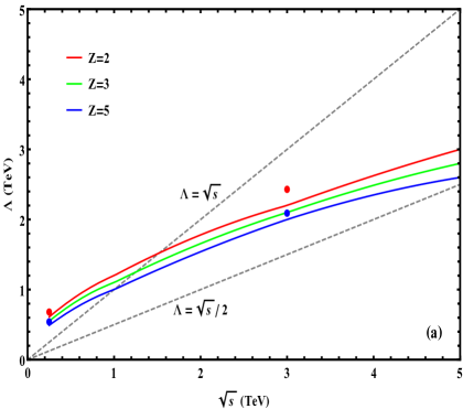
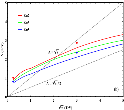
Figure 12: Reaches for the new physics scale $\Lambda$ as functions of the $e^{+}e^{-}$ collision energy $\sqrt{s\,}$ with an integrated luminosity $\,\mathcal{L}\!=\!2\,\text{ab}^{-1}$.  Plot (a) depicts the combined sensitivity $\,\mathcal{Z}\!=\!\sqrt{\mathcal{Z}_{\ell\bar{\ell}}^{2}\!+\!\mathcal{Z}_{\nu\bar{\nu}}^{2}\,}\!=(2,\,3,\,5)\sigma$  for unpolarized $e^{\mp}$ beams, as shown by the (red, green, blue) curves. Plot (b) depicts the combined sensitivity $\,\mathcal{Z}\!=\!\!\sqrt{\mathcal{Z}_{\ell\bar{\ell}}^{2}\!+\!\mathcal{Z}_{\nu\bar{\nu}}^{2}\,}\!=\!(2,\,3,\,5)\sigma$,  with $e^{\mp}$ beam polarizations $(P_{L}^{e},\,P_{R}^{\bar{e}})=(90\%,\,65\%)$,  as shown by the (red, green, blue) curves. In each plot, the (red, blue) dots show the $(2\sigma,\,5\sigma)$ reaches with a projected integrated luminosity $\,\mathcal{L}=5\,\text{ab}^{-1}$ at $\sqrt{s\,}=\mathrm{250GeV}$ (CEPC and FCC-ee) and $\sqrt{s\,}=\mathrm{3TeV}$ (CLIC). For reference, we also show the lines $\,\Lambda\!=\!\sqrt{s\,}$  and $\,\Lambda\!=\!\sqrt{s\,}/2$  in each plot.

We present in Fig. 12 the sensitivity reaches for the new physics scale $\Lambda$ as functions of the collision energy $\sqrt{s\,}$,  with a universal integrated luminosity $\,\mathcal{L}=2\,\text{ab}^{-1}$.  It compares our results for the unpolarized and polarized cases in plots (a) and (b), respectively, assuming $(P_{L}^{e},\,P_{R}^{\bar{e}})=(90\%,\,65\%)$ for the polarized electron and positron beams in the plot (b). In each plot, we show the limits $\mathcal{Z}=(2,\,3,\,5)\sigma$ by the (red, green, blue) curves, where the signal significance $\,\mathcal{Z}\!=\!\!\sqrt{\mathcal{Z}_{\ell\bar{\ell}}^{2}\!+\!\mathcal{Z}_{\nu\bar{\nu}}^{2}\,}$  combines both $\,\ell^{-}{\ell}^{+}\gamma$  and $\,\nu\bar{\nu}\gamma$  channels. For comparison, we further present the sensitivity reaches with a projected integrated luminosity $\,\mathcal{L}=5\,\text{ab}^{-1}$ at $\sqrt{s\,}=\mathrm{250\,GeV}$ (CEPC and FCC-ee) and $\sqrt{s\,}=\mathrm{3\,TeV}$ (CLIC), shown as (red, blue) dots at $(2\sigma,\,5\sigma)$ level. We see that electron/positron beam polarizations can improve significantly the sensitivity reaches for the new physics scale. For reference, we also draw the dashed lines of $\,\Lambda\!=\!\sqrt{s\,}$  and $\,\Lambda\!=\!\sqrt{s\,}/2$  in each plot.

6 . Conclusions

As we have discussed in this work, the reaction $\,e^{+}e^{-}\!\!\rightarrow\!Z\gamma$  provides a rare opportunity to probe an effective dimension-8 operator in the SMEFT. The $ZV\gamma$ vertices ($V\!=\!Z,\gamma$) have no tree-level SM contributions, and nor do they receive any contributions from dimension-6 operators, opening up the possibility of probing the new physics scale associated with the dimension-8 operator. Such dimension-8 operators invoke the Higgs doublets and are connected to the Higgs boson and the spontaneous electroweak symmetry breaking. We have presented a general analysis of the angular distributions for $Z\gamma$ production in the lab frame and for $\,Z\!\!\rightarrow\!\ell^{+}\ell^{-}$  in the $Z$ rest frame to identify distinctive angular distributions and cuts that maximize the statistical sensitivity to the possible new physics scale $\Lambda$, either including only the ${\cal O}(\Lambda^{\!-4})$ contributions that interfere with the SM contributions, or including together the ${\cal O}(\Lambda^{\!-8})$ term of the dimension-8 operator for its full contribution.

As seen in Fig. 8(b) and Tables 2-3, the prospective sensitivities to $\,\Lambda\,$ extend into the multi-TeV range. As expected from the energy dependences of the dimension-8 contributions to the cross section for $\,e^{+}e^{-}\!\!\rightarrow\!Z\gamma$,  Eqs.(40) and (44) show that the prospective sensitivities increase with the collision energy $\!\sqrt{s\,}$, but much slower with the integrated luminosity $\mathcal{L}$ . So taking a constant integrated luminosity in our current tables and figures is a fairly sensible assumption for the simplicity of our presentation. Rescaling the sensitivity reaches to a different $\mathcal{L}$ is straightforward as shown by the (blue, red) dots in Fig. 8(b) and Fig. 12. The sensitivities at the $(2\sigma,\,3\sigma,\,5\sigma)$ levels of significances are not greatly different, as discussed in the text and seen by comparing the (red, green, blue) curves in Fig. 8(b) and Fig. 12.

We have also drawn in Fig. 8 the two reference lines $\,\Lambda\!=\!\sqrt{s\,}$  and $\,\Lambda\!=\!\sqrt{s\,}/2$ .  In general, one would expect the SMEFT approach to be suitable only for energy scales that are small compared to $\Lambda\,$.  However, the way that we have defined $\Lambda$ in Eq.(1) of this paper corresponds to the true new physics scale $\,\tilde{\Lambda}\,$ only if the unknown coefficient $c_{j}$ has a magnitude of unity. If, on the other hand, the true magnitude of $\,c_{j}\!\gg\!1$ GNDA , the true new physics scale $\,\tilde{\Lambda}$  could be sizably larger than the value of $\,\Lambda\,$ extracted from our analysis, and the SMEFT approach would have broader applicability.

We have studied the effect of including the reaction $e^{-}e^{+}\!\!\rightarrow\!Z\gamma$ with invisible decay channel $Z\!\rightarrow\!\nu\bar{\nu}$ in Section 4. We have presented the sensitivities of this channel in Table 5 and Table 6, and derived the combined new physics reaches for both the leptonic and invisible channels $\ell^{-}\ell^{+}\gamma$ and $\nu\bar{\nu}\gamma$ .  We found that the sensitivity of the invisible channel is comparable to that of the lepton channel (cf. Table 5). Then, we demonstrated in Section 5 that including the electron/prostrion beam polarizations can further improve significantly the signal sensitivities. We have presented our findings for the polarized case in Fig.12(b), to be compared with the unpolarized case in Fig.12(a). We have summarized the $2\sigma$ and $5\sigma$ bounds on the new physics scale $\,\Lambda\,$ in Table 7, including the combined reaches of both leptonic and invisible channels.

In summary, we have presented here the sensitivity reaches for the new physics scale $\,\Lambda$  in nTGCs using the reaction $e^{-}e^{+}\!\!\rightarrow\!Z\gamma$ with both leptonic and invisible $Z$ decays, and including their combinations in Table 6 and Fig.12(a). In addition, we have presented in Table 7 and Fig.12(b) the improved sensitivities obtainable with polarized $e^{-}$ and $e^{+}$ beams. Comparing Tables 7 and 6, we see that for collider energies $\sqrt{s}=(250\!-\!1000)$ GeV, using polarized $e^{\mp}$ beams can enhance the sensitivity reaches of $\Lambda$ significantly, by about $(47\!-\!25)\%$ [$(47\!-20\!)\%$] for the $2\sigma$ [$5\sigma$] limits; while for $\sqrt{s}=(3\!-\!5)$ TeV, the polarization effects are much smaller, giving an enhancement around $(18\!-\!10)\%$ [$(5\!-\!8)\%$] for the $2\sigma$ [$5\sigma$] limits.

Finally, it is interesting to compare the sensitivity to the dimension-8 coefficient found here with that found previously in studies of the dimension-8 operator contributions to light-by-light scattering and the process $\,gg\!\rightarrow\!\gamma\gamma$  at the LHC. The former is sensitive to a dimension-8 scale that is ${\cal O}(100)$ GeV gaga-gaga , whereas the latter is sensitive to a dimension-8 scale that is ${\cal O}(1)$ TeV gg-gaga . The dimension-8 operators studied in those analyses contain gauge fields only and differ from what we studied here, hence they probe very different aspects of dimension-8 physics. However, it is encouraging that we have found in this work that future $e^{+}e^{-}$ colliders (such as the CEPC, FCC-ee, ILC, and CLIC) may be able to provide very competitive sensitive probes of the scale of new physics. We therefore encourage further detailed studies of the reaction $\,e^{+}e^{-}\!\!\!\rightarrow\!\!Z\gamma$  by our experimental colleagues.

Appendix

Appendix A . Helicity Amplitudes for $Z\gamma$ Production with $\mathbf{Z}$ Decays

In this Appendix we present the helicity amplitudes for the production process $e^{-}e^{+}\!\rightarrow Z\gamma$, and then we include leptonic $Z$ decays. These results are used in the analyses of Sections 2 and 3 of the main text.

A.1 . Helicity Amplitudes for $Z\gamma$ Production

The helicity amplitudes for $\,e^{-}(p_{1})e^{+}(p_{2})\rightarrow Z(q_{1},\epsilon_{\lambda})\gamma(q_{2},\epsilon_{\lambda^{\prime}})$  can be written as

$$\mathcal{T}^{ss^{\prime}}_{\lambda\lambda^{\prime}}\! = \bar{v}^{s^{\prime}}\!(p_{2})\!\left[\!\frac{e^{2}}{\,s_{W}c_{W}\,}\!\!\left(\!\!\frac{\,\not{\epsilon}_{\lambda^{\prime}}^{*}(q_{2})(\not{q}_{1}\!\!-\!\not{p}_{1})\not{\epsilon}_{\lambda}^{*}(q_{1})\,}{t}+\frac{\,\not{\epsilon}_{\lambda}^{*}(q_{1})(\not{q}_{2}\!\!-\!\not{p}_{1})\not{\epsilon}_{\lambda^{\prime}}^{*}(q_{2})\,}{u}\!\right)\right.$$ (74)

$$\left.\hskip 39.83385pt-\frac{\,\mathrm{i}2M_{Z}^{2}\,}{\,\Lambda^{4}\,}\epsilon^{\mu\nu\alpha\beta}\gamma_{\mu}\epsilon_{\lambda,\nu}^{*}(q_{1})\epsilon_{\lambda^{\prime}\!,\alpha}^{*}(q_{2})q_{2\beta}\!\right]\!\!\left(c_{L}P_{L}\!\!+\!c_{R}P_{R}\right)\!u^{s}(p_{1})\,,\hskip 36.98857pt$$

where we have used the standard spinor notations $u^{s}(p_{1})$ and $\bar{v}^{s^{\prime}}\!(p_{2})$ PeskinBook for the initial-state $\,e^{-}$ and $e^{+}$,  and $(\epsilon_{\lambda},\,\epsilon_{\lambda^{\prime}})$ denote the polarization vectors of the final-state gauge bosons $(Z,\,\gamma)$.  In the above, $\,P_{L,R}=\mbox{$\frac{\,{1}\,}{2}$}(1\mp\gamma_{5})\,$ are the chirality projection operators, and the coefficients  $(c_{L},\,c_{R})=(s_{W}^{2}\!-\!\mbox{$\frac{\,{1}\,}{2}$},\,s_{W}^{2})$  arise from the (left-, right)-handed gauge couplings of electrons to the $Z$ boson. In the above, we have used the Mandelstam variables $\,t=(p_{1}\!-q_{1})^{2}=-\mbox{$\frac{\,{1}\,}{2}$}(s\!-\!M_{Z}^{2})(1\!-\cos\!\theta)\,$ and $\,u=(p_{1}\!-q_{2})^{2}=-\mbox{$\frac{\,{1}\,}{2}$}(s\!-\!M_{Z}^{2})(1\!+\cos\!\theta)\,$.

In Eq.(7) we defined the momenta of the final-state particles $Z(q_{1})\gamma(q_{2})$ as $\,q_{1}=(E_{Z},\,q\sin\!\theta,\,0,\,q\cos\!\theta)$  and $\,q_{2}=q(1,\,-\sin\!\theta,\,0,\,-\cos\!\theta)$.  Then, we can express the three polarization vectors $\epsilon_{\lambda}(q_{1},\theta)$ of the $Z$ boson as follows:

$$\epsilon_{\pm}^{Z}(\theta) = \mbox{$\frac{\,{1}\,}{\sqrt{2\,}\,}$}\!\left(0,\mp{\cos\!\theta},\,-{\mathrm{i}},\,\pm{\sin\!\theta}\right)\!,$$ (75a)

$$\epsilon_{0}^{Z}(q_{1},\theta) = \mbox{$\frac{\,{1}\,}{M_{Z}}$}\!\left(q_{1},\,E_{Z}{\sin\!\theta},\,0,\,E_{Z}{\cos\!\theta}\right)\!,$$ (75b)

where $E_{Z}=\sqrt{q_{1}^{2}\!+\!M_{Z}^{2}\,}$.  The final-state photon has two transverse polarization vectors that are similar to those of the $Z$ boson,

$$\epsilon_{\pm}^{\gamma}(\theta)=\epsilon_{\pm}^{Z}(\theta\!+\!\pi)=\epsilon_{\mp}^{Z}(\theta)\,.\,$$ (76)

The first two terms in Eq.(74) arise from the SM contributions via the $t$- and $u$-channel exchanges, respectively, while the third term is contributed by the dimension-8 operator. For the final-state $Z(\lambda)\gamma(\lambda^{\prime})$ helicity combinations $\lambda\lambda^{\prime}\!=\!(--,-+,+-,++)$ and $\lambda\lambda^{\prime}\!=\!(0-,0+)$,  we compute the SM contributions to the scattering amplitudes as follows:

$$\mathcal{T}_{\text{sm}}^{ss^{\prime}\!,\text{T}}\!\!\left\lgroup\!\!\begin{array}[]{cc}--&-+\\ +-&++\\ \end{array}\!\!\right\rgroup\!\! = \frac{2e^{2}}{\,s_{W}c_{W}(s\!-\!M_{Z}^{2})\,}\!\!\left\lgroup\!\!\begin{array}[]{ll}\left(e_{L}\!\cot\!\frac{\theta}{2}\!-\!e_{R}\!\tan\!\frac{\theta}{2}\right)\!M_{Z}^{2}{}&\left(-e_{L}\!\cot\!\frac{\theta}{2}\!+\!e_{R}\!\tan\!\frac{\theta}{2}\right)\!s\\[5.69054pt] \left(e_{L}\!\tan\!\frac{\theta}{2}\!-\!e_{R}\!\cot\!\frac{\theta}{2}\right)\!s&\left(-e_{L}\!\tan\!\frac{\theta}{2}\!+\!e_{R}\!\cot\!\frac{\theta}{2}\right)\!M_{Z}^{2}\end{array}\!\!\right\rgroup\!\!,\hskip 36.98857pt$$ (77e)

$$\mathcal{T}_{\text{sm}}^{ss^{\prime}\!,\text{L}}(0-,0+) = \frac{\,2\sqrt{2}(e_{L}\!\!+\!e_{R})e^{2}M_{Z}\sqrt{s\,}\,}{\,s_{W}c_{W}(s\!-\!M_{Z}^{2})\,}\left(1,\,-1\right),$$ (77f)

where $\,(e_{L},\,e_{R})=(c_{L}\delta_{\!s,-\frac{1}{2}},\,c_{R}\delta_{\!s,\frac{1}{2}})$,  with the subscript index $\,s=\mp\mbox{$\frac{\,{1}\,}{2}$}$  denoting the initial-state electron helicities. For the massless initial-state $e^{-}$ and $e^{+}$, we have $s=-s^{\prime}$.  We note that, in Eq.(77e), the identical-helicity amplitudes $\,\mathcal{T}_{\text{sm}}^{ss^{\prime}\!,\text{T}}(\pm\pm)$  in the diagonal entries are proportional to $M_{Z}^{2}$ (unlike the off-diagonal entries, which are $\propto s$ ). This is expected because the identical-helicity amplitudes should vanish exactly in the massless limit $M_{Z}\!\rightarrow\!0$,  after ignoring the tiny electron mass, as in the pair-annihilation process $\,e^{-}e^{+}\!\rightarrow\!\gamma\gamma$  in QED PeskinBook . Hence the non-zero amplitudes have asymptotic behaviors  $\mathcal{T}_{\text{sm}}^{ss^{\prime}\!,\text{T}}(\pm\pm)\propto M_{Z}^{2}/s$ .

Next, we compute the corresponding helicity amplitudes from the new physics contributions of the dimension-8 operator, which are as follows:

$$\mathcal{T}_{(8)}^{ss^{\prime}\!,\text{T}}\!\!\left\lgroup\!\!\begin{array}[]{cc}--&-+\\ +-&++\\ \end{array}\!\!\right\rgroup\! = \frac{\,(e_{L}\!\!+\!e_{R})\sin\!\theta M_{Z}^{2}(s\!-\!M_{Z}^{2})\,}{\Lambda^{4}}\!\!\left\lgroup\!\begin{array}[]{cr}1{}&0\\[2.84526pt] 0{}&-1\end{array}\!\right\rgroup\!\!,$$ (78e)

$$\mathcal{T}_{(8)}^{ss^{\prime}\!,\text{L}}(0-,0+) = \frac{\,\sqrt{2}M_{Z}(s\!-\!M_{Z}^{2})\sqrt{s}\,}{\Lambda^{4}}\!\left(\!e_{L}\!\sin^{2}\!\frac{\theta}{2}\!-e_{R}\!\cos^{2}\!\frac{\theta}{2},~{}e_{R}\!\sin^{2}\!\frac{\theta}{2}\!-e_{L}\!\cos^{2}\!\frac{\theta}{2}\right)\!.\hskip 42.67912pt$$ (78f)

We note that in Eq.(78e) the off-diagonal amplitudes $\mathcal{T}_{(8)}^{ss^{\prime}\!,\text{T}}(-+)$ and $\mathcal{T}_{(8)}^{ss^{\prime}\!,\text{T}}(-+)$ vanish exactly. This can be understood by noting that the $Z\gamma Z^{*}$ vertex [cf. Eqs.(6) and (74)] contains the rank-4 antisymmetric tensor $\epsilon^{\mu\nu\alpha\beta}$, which contracts with the $Z$ and $\gamma$ polarization vectors $\epsilon_{\lambda,\nu}^{Z}(\theta)$ and $\epsilon_{\lambda^{\prime}\!,\alpha}^{\gamma}(\theta)$  as in Eq.(74). For the off-diagonal $Z\gamma$ helicity combinations $\,\lambda\lambda^{\prime}=+-,-+$,  we deduce

$$\epsilon^{\mu\nu\alpha\beta}\gamma_{\mu}\epsilon_{\pm,\nu}^{Z*}(\theta)\epsilon_{\mp\!,\alpha}^{\gamma*}(\theta)\,=\,\epsilon^{\mu\nu\alpha\beta}\gamma_{\mu}\epsilon_{\pm,\nu}^{Z*}(\theta)\epsilon_{\pm\!,\alpha}^{Z*}(\theta)\,=\,0\,,$$ (79)

according to Eq.(76).

A.2 . Helicity Amplitudes Including $\mathbf{Z}$ Decays

In this Appendix we incorporate the leptonic decays of the $Z$ boson. We first consider $Z$ decay in its rest frame, $Z\!\rightarrow\!\ell^{-}(k_{1})\ell^{+}(k_{2})$, where the final-state leptons have momenta:

$$k_{1} = k(1,\,\sin\!\theta_{*}\cos\phi_{*},\,\sin\!\theta_{*}\sin\!\phi_{*},\,\cos\!\theta_{*})\,,$$

$$k_{2} = k(1,-\sin\theta_{*}\cos\phi_{*},-\sin\theta_{*}\sin\phi_{*},-\cos\theta_{*})\,,$$

where the leptons are treated as effectively massless and $\,k=|\vec{k}_{1}\!|\simeq\mbox{$\frac{\,{1}\,}{2}$}M_{Z}$ . In the $Z$ rest frame, the massless lepton spinors are defined as follows,

$$u_{+}(k_{1}) = \sqrt{2k}\!\left(0,\,0,\,e^{-\frac{\mathrm{i}\phi_{*}}{2}}\!\cos\!\frac{\theta_{*}}{2},\,e^{\frac{\mathrm{i}\phi_{*}}{2}}\!\sin\!\frac{\theta_{*}}{2}\right)\!,$$

$$u_{-}(k_{1}) = \sqrt{2k}\!\left(-e^{-\frac{\mathrm{i}\phi_{*}}{2}}\!\sin\!\frac{\theta_{*}}{2},\,e^{\frac{\mathrm{i}\phi_{*}}{2}}\!\cos\!\frac{\theta_{*}}{2},\,0,\,0\right)\!,$$

$$v_{+}(k_{2}) = \sqrt{2k}\!\left(e^{-\frac{\mathrm{i}\phi_{*}}{2}}\!\cos\!\frac{\theta_{*}}{2},\,e^{\frac{\mathrm{i}\phi_{*}}{2}}\!\sin\!\frac{\theta_{*}}{2},\,0,\,0\right)\!,$$

$$v_{-}(k_{2}) = \sqrt{2k}\!\left(0,\,0,\,e^{-\frac{\mathrm{i}\phi_{*}}{2}}\!\sin\!\frac{\theta_{*}}{2},\,-e^{\frac{\mathrm{i}\phi_{*}}{2}}\!\cos\!\frac{\theta_{*}}{2}\!\right),$$

where $u_{+}$ ($u_{-}$) correspond to spin-up (-down) and $v_{+}$ ($v_{-}$) correspond to spin-down (-up) along their directions of motion in Eq.(LABEL:eq:k1k2).

Then, we write down the left-handed and right-handed spinor currents in the $Z$ boson rest frame,

$$\widetilde{C}_{L}^{\mu} = \bar{v}_{L}\gamma^{\mu}u_{L}=M_{Z}\!\left(0,\,-\cos\!\theta_{*}\!\cos\!\phi_{*}\!\!-\!\mathrm{i}\sin\!\phi_{*},\,-\cos\!\theta_{*}\!\sin\!\phi_{*}\!\!+\!\mathrm{i}\cos\!\phi_{*},\,\sin\!\theta_{*}\right)\!,\hskip 45.5244pt$$ (82a)

$$\widetilde{C}_{R}^{\mu} = \bar{v}_{R}\gamma^{\mu}u_{R}=M_{Z}\!\left(0,\,-\cos\!\theta_{*}\!\cos\!\phi_{*}\!\!+\mathrm{i}\sin\!\phi_{*},\,-\cos\!\theta_{*}\!\sin\!\phi_{*}\!\!-\mathrm{i}\cos\!\phi_{*},\,\sin\!\theta_{*}\right)\!,$$ (82b)

where $\,(u_{L},\,u_{R})=(u_{-},\,u_{+})\,$ and $\,(v_{L},\,v_{R})=(v_{+},\,v_{-})\,$.  After making a Lorentz boost $\hat{L}$ back to the laboratory frame (i.e., the c.m. frame of the $Z\gamma$ pair) and rotating the axis $z^{*}$ back to the axis $z$ by the rotation $\hat{R}$,  we have new currents $\,C_{L,R}^{\mu}=\hat{R}\hat{L}\widetilde{C}_{L,R}^{\mu}$  in the lab frame. The Lorentz boost $\hat{L}$ acts on the (0, 3) components, with $\,\hat{L}_{00}\!=\!\hat{L}_{33}\!=\gamma$  and $\,\hat{L}_{03}\!=\!\hat{L}_{30}\!=\gamma\beta$ ,  where $(\beta,\,\gamma)=(p_{Z}/E_{Z},\,E_{Z}/M_{Z})$.  The rotation matrix $\hat{R}$ acts on the (1, 3) components, with elements $\,\hat{R}_{11}\!=\!\hat{R}_{33}\!=\cos\!\theta$  and $\,\hat{R}_{13}\!=\!-\hat{R}_{31}\!=\sin\!\theta$.  Thus, we can derive the currents $\,C_{L,R}^{\mu}\,$ and express them in terms of $Z$ boson polarization vectors,

$$C_{L}^{\mu} = M_{Z}\!\left(\!\sin\!\theta_{*}\epsilon_{0}^{Z}-\sqrt{2}\sin^{2}\!\frac{\,\theta_{*}}{2}e^{-\mathrm{i}\phi_{*}}\epsilon_{+}^{Z}-\sqrt{2}\cos^{2}\!\frac{\,\theta_{*}}{2}e^{\mathrm{i}\phi_{*}}\epsilon_{-}^{Z}\right)\!,\hskip 45.5244pt$$ (83a)

$$C_{R}^{\mu} = M_{Z}\!\left(\!\sin\!\theta_{*}\epsilon_{0}^{Z}+\sqrt{2}\cos^{2}\!\frac{\,\theta_{*}}{2}e^{-\mathrm{i}\phi_{*}}\epsilon_{+}^{Z}+\sqrt{2}\sin^{2}\!\frac{\,\theta_{*}}{2}e^{\mathrm{i}\phi_{*}}\epsilon_{-}^{Z}\right)\!.$$ (83b)

Next, we can obtain the amplitude for $\,e^{-}e^{+}\!\!\rightarrow\!\ell^{-}\ell^{+}\gamma$  by replacing the $Z$ polarization vector $\epsilon_{\lambda}^{*\mu}(q_{1})$ in Eq.(74) with $\,C_{L,R}^{\mu}(q_{1})\mathcal{D}_{Z}$, where $\mathcal{D}_{Z}=1/(q_{1}^{2}\!-\!M_{Z}^{2}\!+\!\mathrm{i}M_{Z}\Gamma)$  is from the $Z$ propagator. Since $\,q_{1\mu}C_{L,R}^{\mu}(q_{1})\!=0$, we can drop the $\,q_{1}^{\mu}q_{1}^{\nu}\,$ term in the $Z$-propagator. Then, we derive the $\ell^{-}\ell^{+}\gamma$ amplitude as follows,

$$\mathcal{T}^{ss^{\prime}}_{\sigma\sigma^{\prime}\!\lambda}(\ell\bar{\ell}\gamma)\! = \frac{\,ef_{L,R}\mathcal{D}_{\!Z}\,}{s_{W}c_{W}}\bar{v}^{s^{\prime}}\!(p_{2})\!\!\left[\!\frac{e^{2}}{\,s_{W}c_{W}\,}\!\!\left(\!\!\frac{\,\not{\epsilon}_{\lambda}^{*}(q_{2})(\not{q}_{1}\!\!-\!\not{p}_{1})\not{C}_{L,R}^{*}(q_{1})\,}{t}+\frac{\,\not{C}_{L,R}^{*}(q_{1})(\not{q}_{2}\!\!-\!\not{p}_{1})\not{\epsilon}_{\lambda}^{*}(q_{2})\,}{u}\!\right)\right.\hskip 14.22636pt$$ (84)

$$\left.\hskip 39.83385pt-\frac{\,\mathrm{i}2M_{Z}^{2}\,}{\,\Lambda^{4}\,}\epsilon^{\mu\nu\alpha\beta}\gamma_{\mu}C_{L,R;\nu}^{*}(q_{1})\epsilon_{\lambda\!,\alpha}^{*}(q_{2})q_{2\beta}\!\right]\!\!\left(c_{L}P_{L}\!\!+\!c_{R}P_{R}\right)\!u^{s}(p_{1})\,,\hskip 28.45274pt$$

where $\,(\sigma,\,\sigma^{\prime}\!,\,\lambda)$  denote the helicities of the final-state particles $(\ell^{-},\,\ell^{+},\,\gamma)$ with $\,\sigma=-\sigma^{\prime}\,$ for massless leptons, and we have defined the coefficients $\,(f_{L},\,f_{R})=(c_{L}\delta_{\!\sigma,-\frac{1}{2}},\,c_{R}\delta_{\!\sigma,\frac{1}{2}})$.

Substituting Eq.(83) into Eq.(84), we can express the amplitude (74) in terms of the helicity amplitudes (77)-(78) of Appendix A.1,

$$\mathcal{T}^{ss^{\prime}}_{\sigma\sigma^{\prime}\!\lambda}\!(\ell\bar{\ell}\gamma) = \frac{\,eM_{Z}\mathcal{D}_{Z}\,}{s_{W}c_{W}}\left[\sqrt{2\,}e^{\mathrm{i}\phi_{*}}\!\!\left(\!f_{R}^{\sigma}\cos^{2}\!\frac{\,\theta_{*}}{2}\!-f_{L}^{\sigma}\!\sin^{2}\!\frac{\,\theta_{*}}{2}\!\right)\!\mathcal{T}_{ss^{\prime}}^{T}(+\lambda)\right.$$

$$\left.+\sqrt{2\,}e^{-i\phi_{*}}\!\!\left(\!f_{R}^{\sigma}\sin^{2}\!\frac{\,\theta_{*}}{2}\!-f_{L}^{\sigma}\!\cos^{2}\!\frac{\,\theta_{*}}{2}\!\right)\!\mathcal{T}_{ss^{\prime}}^{T}(-\lambda)+(f_{R}^{\sigma}\!+\!f_{L}^{\sigma})\sin\!\theta_{*}\mathcal{T}_{ss^{\prime}}^{L}(0\lambda)\right]\!,\hskip 36.98857pt$$

where $\mathcal{T}_{ss^{\prime}}^{T}(\pm\lambda)$ and $\mathcal{T}_{ss^{\prime}}^{L}(0\lambda)$ are the on-shell helicity amplitudes of $\,e^{-}e^{+}\!\!\rightarrow Z\gamma$ ,

$$\mathcal{T}_{ss^{\prime}}^{T}(\pm\lambda) = \mathcal{T}^{ss^{\prime}\!,T}_{\text{sm}}(\pm\lambda)+\mathcal{T}^{ss^{\prime}\!,T}_{(8)}(\pm\lambda)\,,$$

$$\mathcal{T}_{ss^{\prime}}^{L}(0\lambda) = \mathcal{T}^{ss^{\prime}\!,L}_{\text{sm}}(0\lambda)+\mathcal{T}^{ss^{\prime}\!,L}_{(8)}(0\lambda)\,,$$

which sum up the contributions from both the SM and the dimension-8 operator as derived in Eqs.(77)-(78) of Appendix A.1. From Eq.(A.2), we see that the full cross section for $\,e^{-}e^{+}\!\!\rightarrow\!\ell^{-}\ell^{+}\gamma$  depends on the angle $\,\phi_{*}$,  due to the interference between the terms with different $Z$ boson helicities $\lambda^{\prime}\!=+,-,0$ .  Eq.(A.2) also exhibits the $\,\theta_{*}$ dependence associated with each $Z$ boson helicity. We have used Eqs.(A.2)-(A.2) in the analysis of angular observables in Section 3.

Appendix B . Sensitivities $\mathcal{Z}_{4}$ and $\mathcal{Z}_{8}$ have Negligible Correlation

In this Appendix, we prove that the two statistical significances denoted by $\mathcal{Z}_{4}$ and $\mathcal{Z}_{8}$ in Sections 3.2.1 and 3.2.2 have negligible correlation. Hence, their combination $\,\mathcal{Z}\!=\!\!\sqrt{\mathcal{Z}_{4}^{2}\!+\!\mathcal{Z}_{8}^{2}\,}$  is well justified. In the following, we will first demonstrate that there is no overlap or double-counting between the two signals $S_{I}$ (for $\mathcal{Z}_{4}$) and $S_{II}$ (for $\mathcal{Z}_{8}$). Then, we further prove that there is negligible correlation between the corresponding background events $B_{I}$ and $B_{II}$.

We first explain why there is no correlation between the two signals $S_{I}$ and $S_{II}$, as analyzed in Sections 3.2.1 and 3.2.2. We presented the angular distributions of $\phi_{*}$ in Eq.(21) and Fig. 4. It is clear that for the distributions $\,f_{\phi_{*}}^{0,2}$, the constant terms mainly dominate $\,f_{\phi_{*}}^{0,2}$, and all the $\phi_{*}$ terms are suppressed by $M_{Z}/\!\sqrt{s}$ and have no significant effect. But in the distribution $\,f_{\phi_{*}}^{1}$  the $\cos\phi_{*}$ term is enhanced by $\sqrt{s}/M_{Z}$ and dominates $\,f_{\phi_{*}}^{1}$, while all other terms are negligible. We note that for computing the significance $\mathcal{Z}_{4}$ in Eq.(27),  the signal $S_{I}$ and the SM background error $\,\Delta_{B_{I}}$ [in Eqs.(24),(26)] originate from the $\cos\!\phi_{*}$ term of $\,f_{\phi_{*}}^{1}$ and the constant term of $\,f_{\phi_{*}}^{0}$ [in Eq.(21)], respectively. From the above explanation and the discussion around Eq.(25), we see that the constant terms in $\,f_{\phi_{*}}^{1,2}$ are strongly cancelled in the signal $S_{I}$, so $S_{I}$ originates from the $\cos\!\phi_{*}$ term of $\,f_{\phi_{*}}^{1}$ under the asymmetric integration (23) [and thus (25)]. Next, we inspect the significance $\mathcal{Z}_{8}$ defined in Eq.(32). It contains the signal $S_{II}$ and the SM background error $\,\Delta_{B_{II}}$ in Eq.(33), which originate from the constant terms of $\,f_{\phi_{*}}^{1,2}$ and $\,f_{\phi_{*}}^{0}$ in Eq.(21), respectively. For $\mathcal{Z}_{8}$, our integrations over the full range of $\phi_{*}$ are uniform and receive no cancellation for the constant terms in $\,f_{\phi_{*}}^{1,2}$ and $\,f_{\phi_{*}}^{0}$,  but integrations over the terms of $\cos\phi_{*}$ and $\cos 2\phi_{*}$ vanish identically. Hence, the significance $\mathcal{Z}_{8}$ only extracts the constant terms of $\,f_{\phi_{*}}^{1,2}$ and $\,f_{\phi_{*}}^{0}$ for $S_{II}$ and $\,\Delta_{B_{II}}$.  This is contrary to the case of $\mathcal{Z}_{4}$, where the signal $S_{I}$ extracts the $\cos\phi_{*}$ term alone. The above analysis proves that for the significances $\mathcal{Z}_{4}$ and $\mathcal{Z}_{8}$, their corresponding signals $S_{I}$ and $S_{II}$ originate from totally different parts of the $\phi_{*}$ distributions. This means that the two subgroups of signal events included in $S_{I}$ and $S_{II}$ are different and do not overlap. Hence, the signal samples $S_{I}$ and $S_{II}$ have no double-counting and are not correlated.

Because of the fact that $S_{I}$ and $S_{II}$ contain two different subgroups of signal events without overlap, it is clear that any other cuts (such as the $\theta$ cut we used in Table 1) cannot cause extra correlation between $S_{I}$ and $S_{II}$. To make this fully obvious, we consider the angular distributions respect to both $\,\phi_{*}\,$ and $\,\theta\,$ for instance, namely, the differential cross sections $\mathrm{d}^{2}\sigma_{j}/\mathrm{d}\phi_{*}\mathrm{d}\theta$ (with $j=0,1,2$), where $(\sigma_{0},\,\sigma_{1},\,\sigma_{2})$ correspond to the contributions from the SM, the $O(\Lambda^{-4})$ term, and the $O(\Lambda^{-8})$ term, respectively. Expanding in the small parameter $M_{Z}/\!\sqrt{s}$,  we can formally write down the structure of $\mathrm{d}^{2}\sigma_{j}/\mathrm{d}\phi_{*}\mathrm{d}\theta$ as follows,

$$\frac{1}{\sigma_{0}}\frac{\mathrm{d}^{2}\sigma_{0}}{\,\mathrm{d}\phi_{*}\mathrm{d}\theta\,} = h_{00}(\theta)+h_{01}(\theta)\cos\!\phi_{*}\frac{M_{Z}}{E\,}+O\!\!\left(\!\frac{M_{Z}^{2}}{E^{2}}\!\right)\!,$$ (87a)

$$\frac{1}{\sigma_{1}}\frac{\mathrm{d}^{2}\sigma_{1}}{\mathrm{d}\phi_{*}\mathrm{d}\theta} = h_{10}(\theta)+h_{11}(\theta)\cos\!\phi_{*}\frac{E}{\,M_{Z}}+h_{12}(\theta)\cos\!2\phi_{*}+O\!\!\left(\!\frac{M_{Z}^{2}}{E^{2}}\!\right)\!,~{}~{}~{}~{}~{}$$ (87b)

$$\frac{1}{\sigma_{2}}\frac{\mathrm{d}^{2}\sigma_{2}}{\mathrm{d}\phi_{*}\mathrm{d}\theta} = h_{20}(\theta)+h_{21}(\theta)\cos\!\phi_{*}\frac{M_{Z}}{E}+O\!\!\left(\!\frac{M_{Z}^{3}}{E^{3}}\!\right)\!,~{}~{}~{}~{}~{}$$ (87c)

where $E=\!\sqrt{s\,}$.  It is clear that $\,{\mathrm{d}^{2}\sigma_{1}}/{\mathrm{d}\phi_{*}\mathrm{d}\theta}$  is dominated by the $\,\cos\!\phi_{*}$ term with coefficient $h_{11}(\theta)$, while ${\mathrm{d}^{2}\sigma_{0}}/{\mathrm{d}\phi_{*}\mathrm{d}\theta}$ and ${\mathrm{d}^{2}\sigma_{2}}/{\mathrm{d}\phi_{*}\mathrm{d}\theta}$ are dominated by the $E$-independent terms $h_{00}(\theta)$ and $h_{20}(\theta)$.  Integrating Eq.(87) over $\,\theta\,$, we obtain the angular distributions $f_{\phi_{*}}^{0,1,2}$ in Eq.(21). We note that the signal $S_{I}$ (for $\mathcal{Z}_{4}$) is given by the term $h_{11}(\theta)\cos\!\phi_{*}$ after the integration over $\,\theta$  and the asymmetric integration over $\,\phi_{*}\,$,  while the signal $S_{II}$ (for $\mathcal{Z}_{8}$) comes from the $E$-independent terms $h_{10}(\theta)$ and $h_{20}(\theta)$ in ${\mathrm{d}^{2}\sigma_{1}}/{\mathrm{d}\phi_{*}\mathrm{d}\theta}$ ,  after integrating over $\,\theta$  and $\,\phi_{*}\,$.  For the $\,\theta$  integration, we can add different $\,\theta$  cuts on the integrations of $h_{11}(\theta)$ and $h_{10,20}(\theta)$, respectively, as in Table 1. The key point is that the term $h_{11}(\theta)$ and the terms $h_{10,20}(\theta)$ contain two different subgroups of events without overlap. Hence, the $\,\theta$  cuts (Table 1) cannot cause any correlation between $S_{I}$ and $S_{II}$.

In the following, we further prove that there is negligible statistical correlation between the backgrounds $B_{I}=N_{0}^{b}-N_{0}^{a}$ (for $\mathcal{Z}_{4}$) and $B_{II}=\overline{N}_{0}^{b}+\overline{N}_{0}^{a}$ (for $\mathcal{Z}_{8}$), where $B_{I}$ and $B_{II}$ are defined in Eqs.(26) and (33). We follow the concepts and definitions of statistical errors and correlations given by a standard textbook such as Ref. book . We stress that the following proof is based on pure statistical reasoning only and is completely general, independent of any additional kinematical cuts (such as the cuts on $\theta$ and $\theta_{*}$ distributions).

We denote by $x$ and $y$ two independent observables (such as the event numbers $N_{a}$ and $N_{b}$ in regions (a) and (b) of the $\phi_{*}$ distribution discussed in Section 3.2),

$$x=\overline{x}+\delta_{x}\,,~{}~{}~{}~{}~{}~{}y=\overline{y}+\delta_{y}\,,$$ (88)

where $(\bar{x},\,\bar{y})$ are the statistical means (expectation values) of $(x,\,y)$, and $(\delta_{x},\,\delta_{y})$ denote the corresponding statistical errors. Since $x$ and $y$ are independent of each other by definition, we have $\overline{xy\,}=\overline{x\,}\,\overline{y\,}$.

By definition, we have $\overline{\delta_{x}}=\overline{\delta_{y}}=0$ and $(\,\overline{\delta_{x}^{2}},\,\overline{\delta_{y}^{2}}\,)=(\sigma_{x}^{2},\,\sigma_{y}^{2})$,  where $(\sigma_{x}^{2},\,\sigma_{y}^{2})$ are the corresponding variances whose square-roots $(\sigma_{x},\,\sigma_{y})$ are the so-called standard deviations. The covariance of $(x,\,y)$ is given by

$$\text{Cov}(x,y)\,=\,\overline{(x-\bar{x})(y-\bar{y})}\,=\,\overline{\delta_{x}\delta_{y}}\,=\,\overline{xy\,}-\overline{x\,}\,\overline{y\,}\,=\,0\,,$$ (89)

since $\,\overline{xy\,}=\overline{x\,}\,\overline{y\,}$.

Any observable $\mathcal{O}(x,y)$ can be expanded up to linear order in $(\delta_{x},\,\delta_{y})$:

$$\mathcal{O}(x,y)\,=\,\overline{\mathcal{O}}+\frac{\partial\mathcal{O}}{\partial x}\delta_{x}\!+\frac{\partial\mathcal{O}}{\partial y}\delta_{y}\,.$$ (90)

For the current purpose, we may define the two observables $\mathcal{O}_{+}$ and $\mathcal{O}_{-}$ as follows,

$$\mathcal{O}_{+} \!= x+y\,=\,(\overline{x}+\overline{y})+(\delta_{x}\!+\delta_{y}),$$ (91)

$$\mathcal{O}_{-} \!= x-y\,=\,(\overline{x}-\overline{y})+(\delta_{x}\!-\delta_{y}).$$

Then, we can deduce the variances and covariances of $(\mathcal{O}_{+},\mathcal{O}_{-})$:

$$\sigma_{+}^{2}=\sigma_{-}^{2} = \sigma_{x}^{2}+\sigma_{y}^{2},$$ (92a)

$$\text{Cov}(\mathcal{O}_{+},\mathcal{O}_{-}) = \overline{(\mathcal{O}_{+}\!-\!\overline{\mathcal{O}}_{+})(\mathcal{O}_{-}\!-\!\overline{\mathcal{O}}_{-})}=\overline{(\delta_{x}\!+\!\delta_{y})(\delta_{x}\!-\!\delta_{y})}\hskip 42.67912pt$$ (92b)

$$= \overline{\delta_{x}^{2}}-\overline{\delta_{y}^{2}}\,=\,\sigma_{x}^{2}\!-\sigma_{y}^{2}\,.$$

Thus, we can derive the statistical correlation $\rho$ between $\mathcal{O}_{+}$ and $\mathcal{O}_{-}$ as follows,

$$\rho\,=\,\frac{\,\text{Cov}(\mathcal{O}_{+},\mathcal{O}_{-})\,}{\sigma_{+}\sigma_{-}}\,=\,\frac{~{}\sigma_{x}^{2}\!-\!\sigma_{y}^{2}~{}}{\sigma_{x}^{2}\!+\!\sigma_{y}^{2}}\,.$$ (93)

For our current study, we choose the two independent observables $(x,\,y)$ to be the SM background event numbers $(N_{0}^{b},\,N_{0}^{a})$ in regions (b) and (a) of the $\phi_{*}$ distribution, i.e., $(x,\,y)=(N_{0}^{b},\,N_{0}^{a})$.  Thus, $(\mathcal{O}_{-},\mathcal{O}_{+})=(B_{I},\,B_{II})=(N_{0}^{b}\!-\!N_{0}^{a},\,N_{0}^{b}\!+\!N_{0}^{a})$.  So, we have $(\sigma_{x},\,\sigma_{y})=(\sqrt{N_{0}^{b}},\,\sqrt{N_{0}^{a}})$.  Because our analysis chooses the regions (a) and (b) to have the same size in the $\phi_{*}$ range and the background distribution $f^{0}_{\phi_{*}}$ is nearly flat, we always have $N_{0}^{a}\simeq\!N_{0}^{b}$ . Thus, we can deduce the correlation

$$|\rho|\,=\,\frac{\,|N_{0}^{b}\!-\!N_{0}^{a}|\,}{N_{0}^{b}\!+\!N_{0}^{a}}\ll 1\,.$$ (94)

This means that as long as our choices of regions (a) and (b) obeys the relation $N_{0}^{a}\approx\!N_{0}^{b}\gg|N_{0}^{b}-N_{0}^{a}|$,  the correlation $\,\rho\,$ between the $B_{I}$ and $B_{II}$ can be safely ignored. Hence, $B_{I}$ and $B_{II}$ are independent of each other. Because we already showed in Sec. 3.2.2 that the signals $S_{I}$ and $S_{II}$ in the two analyses are also uncorrelated, the significances $\mathcal{Z}_{4}$ and $\mathcal{Z}_{8}$ are independent of each other.

Furthermore, we can apply additional different cuts on $B_{I}$ and $B_{II}$ (such as the angular cuts on $\theta$ and $\theta_{*}$ distributions) to optimize the significanes $\mathcal{Z}_{4}$ and $\mathcal{Z}_{8}$, respectively. We denote

$$B_{I}=N_{0bI}\!-\!N_{0aI},\,~{}~{}~{}~{}~{}B_{II}=N_{0bII}\!+\!N_{0aII},$$ (95)

where the regions $aI,aII\in a$ and $bI,bII\in b$ .  For any $\,aX\in a\,$ and $\,bY\in b\,$ (with $X,Y=I,II$), we have $\text{Cov}(aX,bY)=\overline{\delta_{aX}\delta_{bY}}=0$  because $a\bigcap b=0$ and thus $aX\bigcap bY\!=0$ .  Thus, we can derive the covariance between the backgrounds $B_{I}$ and $B_{II}$,

$$\text{Cov}(I,II) = \overline{(\delta_{bI}\!-\!\delta_{aI})(\delta_{bII}\!+\!\delta_{aII})}\,=\,\overline{\delta_{bI}\delta_{bII}}\!-\overline{\delta_{aI}\delta_{aII}}$$ (96)

$$= \text{Cov}(bI,bII)\!-\!\text{Cov}(aI,aII)$$

$$= N_{0(bI\bigcap bII)}-N_{0(aI\bigcap aII)}\,,~{}~{}~{}~{}$$

where $N_{0(aI\bigcap aII)}$ denotes the SM background event number in the overlapping region $\,aI\bigcap aII$,  and $N_{0(bI\bigcap bII)}$ gives the background event number in the overlapping region $\,bI\bigcap bII$.  Finally, we derive the correlation between the backgrounds $B_{I}$ and $B_{II}$,

$$\rho\,=\frac{\text{Cov}(I,II)}{\sigma_{I}\sigma_{II}}=\frac{\,N_{0(bI\bigcap bII)}-N_{0(aI\bigcap aII)}\,}{\sqrt{(N_{0aI}\!+\!N_{0bI})(N_{0aII}\!+\!N_{0bII})\,}}\,,$$ (97)

where the variances

$$\sigma_{I}^{2}=\overline{\delta_{aI}^{2}}+\overline{\delta_{bI}^{2}}=N_{0aI}\!+\!N_{0bI}\,,~{}~{}~{}~{}\sigma_{II}^{2}=\overline{\delta_{aII}^{2}}+\overline{\delta_{bII}^{2}}=N_{0aII}\!+\!N_{0bII}\,.\,$$ (98)

Since the cuts imposed in our current analysis are symmetric, we have

$$N_{0(aI\bigcap aII)}\,\approx\,N_{0(bI\bigcap bII)}\,,$$ (99)

and thus $\,|N_{0(bI\bigcap bII)}-N_{0(aI\bigcap aII)}|\ll\sqrt{(N_{0aI}\!+\!N_{0bI})(N_{0aII}\!+\!N_{0bII})\,}\,$.  This leads to the correlation between the backgrounds $B_{I}$ and $B_{II}$,

$$|\rho|\,=\,\frac{\,|N_{0(bI\bigcap bII)}-N_{0(aI\bigcap aII)}|\,}{\sqrt{(N_{0aI}\!+\!N_{0bI})(N_{0aII}\!+\!N_{0bII})\,}}\ll\,1\,.$$ (100)

which is negligible. Here we note that for deriving Eq.(100), we already take into account the effects of additional kinematical cuts (such as the angular cuts on $\theta$ and $\theta_{*}$, etc), which allow the unequal parameter spaces of $\,aI\!\neq\!aII$ and $\,bI\!\neq\!bII$.  This is an extension of our result (94) (with $aI\!=\!aII$ and $\,bI\!=\!bII$) to the general case.

We stress that the above conclusion is based on pure statistical reasoning only. Hence, the fact of $\,|\rho|\!\ll\!1$ is independent of any additional kinematical cuts (such as the cuts on $\theta$ and $\theta_{*}$ distributions).

With the above, we conclude that the significanes $\mathcal{Z}_{4}$ and $\mathcal{Z}_{8}$ are independent of each other. Hence, the combination $\,\mathcal{Z}\!=\!\!\sqrt{\mathcal{Z}_{4}^{2}\!+\!\mathcal{Z}_{8}^{2}\,}$  is well justified.

Acknowledgments
We thank Manqi Ruan for discussing the electron/positron beam polarizations at the linear and circular colliders, and thank him and Kun Liu for discussing the photon energy resolution at the lepton colliders and the LHC. The work of JE was supported in part by United Kingdom STFC Grant ST/P000258/1, in part by the Estonian Research Council via a Mobilitas Pluss grant, and in part by the TDLI distinguished visiting fellow programme. The work of HJH and RQX was supported in part by the National NSF of China (under grants 11675086 and 11835005). HJH is also supported in part by the CAS Center for Excellence in Particle Physics (CCEPP), by the National Key R & D Program of China (No. 2017YFA0402204), by the Shanghai Laboratory for Particle Physics and Cosmology (No. 11DZ2260700), and by the Office of Science and Technology, Shanghai Municipal Government (No. 16DZ2260200).

References

• (1) For recent reviews, see  J. Ellis, “Particle Physics Today, Tomorrow and Beyond”, Int. J. Mod. Phys. A 33 (2018) 1830003 (no.2); and “The Future of High-Energy Collider Physics”, arXiv:1810.11263 [hep-ph].
• (2) W. Buchmuller and D. Wyler, Nucl. Phys. B 268 (1986) 621.
• (3) B. Grzadkowski, M. Iskrzynski, M. Misiak, and J. Rosiek, JHEP 1010 (2010) 085 [arXiv:1008.4884 [hep-ph]].
• (4) For some reviews, see I. Brivio and M. Trott, Phys. Rept. 11 (2018) 002 [arXiv:1706.08945 [hep-ph]]; S. Willenbrock and C. Zhang, Ann. Rev. Nucl. Part. Sci.  64 (2014) 83 [arXiv:1401.0470 [hep-ph]]; D. de Florian et al., [LHC Higgs Cross Section Working Group], arXiv:1610.07922 [hep-ph].
• (5) See, e.g., J. Ellis, V. Sanz, and T. You, JHEP 1407 (2014) 036 [Xiv:1404.3667 [hep-ph]] and JHEP 1503 (2015) 157 [arXiv:1410.7703 [hep-ph]]; J. de Blas, M. Ciuchini, E. Franco, S. Mishima, M. Pierini, L. Reina and L. Silvestrini, JHEP 1612 (2016) 135 [arXiv:1608.01509 [hep-ph]]; C. W. Murphy, Phys. Rev. D 97 (2018) 015007 (no.1) [arXiv:1710.02008 [hep-ph]]; J. Ellis, C. W. Murphy, V. Sanz, and T. You, JHEP 1806 (2018) 146 [arXiv:1803.03252], and references therein.
• (6) J. Ellis, P. Roloff, V. Sanz, and T. You, JHEP 1705 (2017) 096 [arXiv:1701.04804 [hep-ph]].
• (7) See, e.g., J. Ellis and T. You, JHEP 1603 (2016) 089 [arXiv:1510.04561 [hep-ph]; S. F. Ge, H. J. He, and R. Q. Xiao, JHEP 1610 (2016) 007 [arXiv:1603.03385 [hep-ph]]; H. J. He, J. Ren, and W. Yao, Phys. Rev. D 93 (2016) 015003 [arXiv:1506.03302 [hep-ph]]; G. Durieux, C. Grojean, J. Gu, K. Wang, JHEP 1709 (2017) 014 [arXiv:1704.02333 [hep-ph]]; T. Barklow, K. Fujii, S. Jung, R. Karl, J. List, T. Ogawa, M. E. Peskin, and J. Tian, Phys. Rev. D 97 (2018) 053003 [arXiv:1708.08912 [hep-ph]]; and references therein.
• (8) For a general discussion of operators with dimensions $>6$, see: B. Henning, X. Lu, T. Melia, and H. Murayama, JHEP 1708 (2017) 016 [arXiv:1512.03433 [hep-ph]].
• (9) G. J. Gounaris, J. Layssac, and F. M. Renard, Phys. Rev. D 65 (2002) 017302 [arXiv:hep-ph/0005269].
• (10) C. Degrande, JHEP 1402 (2014) 101 [arXiv:1308.6323 [hep-ph]].
• (11) M. Aaboud et al. [ATLAS Collaboration], Phys. Lett. B 775 (2017) 105 [arXiv:1707.04147 [hep-ex]].
• (12) C. Hays, A. Martin, V. Sanz, and J. Setford, JHEP 1902 (2019) 123 [arXiv:1808.00442 [hep-ph]].
• (13) CEPC Study Group, F. An et al., Chin. Phys. C 43 (2019) 043002, no.4, [arXiv:1810.09037 [hep-ex]]; and arXiv:1811.10545 [hep-ex].
• (14) M. Mangano et al., CERN-ACC-2018-0056, http://cds.cern.ch/record/2651294/files/CERN-ACC-2018-0056.pdf.
• (15) K. Fujii et al., arXiv:1710.07621 [hep-ex].
• (16) J. de Blas et al., CERN-TH-2018-267 and CERN-2018-009-M, arXiv:1812.02093 [hep-ph].
• (17) A. Senol, H. Denizli, A. Yilmaz, I. Turk Cakir, K. Y. Oyulmaz, O. Karadeniz, and O. Cakir, Nucl. Phys. B 935 (2018) 365 [arXiv:1805.03475 [hep-ph]].
• (18) J. Ellis, N. E. Mavromatos, and T. You, Phys. Rev. Lett. 118 (2017) 261802 [arXiv:1703.08450 [hep-ph]].
• (19) M. Aaboud et al. [ATLAS Collaboration], Nature Phys.  13 (2017) 852 (no.9), [arXiv:1702.01625 [hep-ex]] and CERN-EP-2016-316;
G. Aad et al. [ATLAS Collaboration], CERN-EP-2019-051, arXiv:1904.03536 [hep-ex].
• (20) J. Ellis and S. F. Ge, Phys. Rev. Lett. 121 (2018) 041801 [arXiv:1802.02416 [hep-ph]].
• (21) B. Bellazzini and F. Riva, Phys. Rev. D98 (2018) 095021 [arXiv:1806.09640 [hep-ph]].
• (22) M. Tanabashi et al., [Particle Data Group], Phys. Rev. D 98 (2018) 030001.
• (23) For a comprehensive review, H. J. He, Y. P. Kuang, C. P. Yuan, arXiv:hep-ph/9704276 and DESY-97-056, in the proceedings of the workshop on “Physics at the TeV Energy Scale”, vol.72, p.119 (Gordon and Breach, New York, 1996). See also, H. J. He and W. B. Kilgore, Phys. Rev. D 55 (1997) 1515; H. J. He, Y. P. Kuang and C. P. Yuan, Phys. Rev. D 51 (1995) 6463; Phys. Rev. D 55 (1997) 3038; H. J. He, Y. P. Kuang and X. Li, Phys. Lett. B 329 (1994) 278; Phys. Rev. D 49 (1994) 4842; Phys. Rev. Lett. 69 (1992) 2619; and references therein.
• (24) B. Ananthanarayan et al., JHEP 1408 (2014) 124 [arXiv:1404.4845 [hep-ph]].
• (25) R. Rahaman and R. K. Singh, Eur. Phys. J. C76 (2016) 539 [arXiv:1604.06677].
• (26) E.g., M. E. Peskin, arXiv:1101.2414 [hep-ph].
• (27) T. Hahn, Comput. Phys. Commun.  140 (2001) 418 [arXiv:hep-ph/0012260].
• (28) V. Shtabovenko, R. Mertig and F. Orellana, Comput. Phys. Commun.  207 (2016) 432 [arXiv:1601.01167 [hep-ph]].
• (29) R. Mertig, M. Bohm and A. Denner, Comput. Phys. Commun.  64 (1991) 345.
• (30) A. G. Cohen, D. B. Kaplan, and A. E. Nelson, Phys. Lett. B 412 (1997) 301 [arXiv:hep-ph/9706275].
• (31) S. F. Ge, H. J. He, and R. Q. Xiao, JHEP 1610 (2016) 007 [arXiv:1603.03385].
• (32) A. M. Sirunyan et al. [CMS Collaboration], JINST 12 (2017) P10003 (no.10) [arXiv:1706.04965 [physics.ins-det]].
• (33) S. Chatrchyan et al. [CMS Collaboration], JINST 8 (2013) P09009 [arXiv:1306.2016 [hep-ex]].
• (34) John I. Marden, “Mathematical Statistics”, by CreateSpace Independent Publishing Platform, 2017. (http://stat.istics.net/MathStat)