Abstract

The explicit expression for the $R$–ratio of electron–positron annihilation into hadrons, which properly accounts for all the effects due to continuation of the spacelike perturbative results into the timelike domain, is obtained at an arbitrary loop level. Several equivalent ways to derive a commonly employed approximation of the $R$–ratio are recapped and the impact of discarded in the latter higher–order $\pi^{2}$–terms on the evaluation of the strong running coupling is elucidated. The obtained results substantially facilitate the theoretical study of electron–positron annihilation into hadrons and the related strong interaction processes. Keywords:  spacelike and timelike domains, hadronic vacuum polarization function, electron–positron annihilation into hadrons, explicit form

1 Introduction

A broad range of topics in particle physics (including electron–positron annihilation into hadrons, inclusive hadronic decays of $\tau$ lepton and $Z$ boson, hadronic contributions to such precise electroweak observables as the muon anomalous magnetic moment and the running of the electromagnetic coupling) is inherently based on the hadronic vacuum polarization function $\Pi(q^{2})$, the Adler function $D(Q^{2})$, and the function $R(s)$. The theoretical study of the aforementioned strong interaction processes factually represents a decisive consistency test of Quantum Chromodynamics (QCD) and entire Standard Model, that puts stringent constraints on a possible new fundamental physics beyond the latter. Additionally, a majority of the processes on hand are of a direct pertinence to the numerous ongoing research programs and the future collider projects, for example, the first phases of Future Circular Collider (FCC) [1] and Circular Electron–Positron Collider (CEPC) [2], International Linear Collider (ILC) [3], Compact Linear Collider (CLIC) [4], as well as E989 experiment at Fermilab [5], E34 experiment at J–PARC [6], MUonE project [7], and many others.

Basically, over the past decades the QCD perturbation theory still remains to be an essential tool for the theoretical investigation of the strong interaction processes. However, leaving aside the irrelevance of perturbative approach to the low–energy hadron dynamics, it is necessary to outline that the QCD perturbation theory and the renormalization group (RG) method can be directly applied to the study of the strong interactions in the spacelike (Euclidean) domain only, whereas the proper description of hadron dynamics in the timelike (Minkowskian) domain substantially relies on the corresponding dispersion relations. In particular, the latter provide the physically consistent way to interrelate the “timelike” experimentally measurable observables (such as the $R$–ratio of electron–positron annihilation into hadrons) with the “spacelike” theoretically computable quantities (such as the Adler function).

In general, the calculation of the explicit expression for the function $R(s)$, which thoroughly incorporates all the effects of continuation of perturbative results from spacelike to timelike domain, represents quite a demanding task. Eventually, this fact forces one to either employ the numerical computation methods or resort to an approximate form of the $R$–ratio, specifically, its truncated re–expansion at high energies. However, the former requires a lot of computational resources and becomes rather sophisticated at the higher loop levels, whereas the latter generates an infinite number of the so–called $\pi^{2}$–terms, which may not necessarily be small enough to be safely neglected at the higher orders and may produce a considerable effect on $R(s)$ even at high energies (a detailed discussion of these issues can be found in, e.g., Refs. [20, 21, 22, 23, 24] as well as Refs. [25, 26] and references therein).

The primary objective of the paper is to obtain, at an arbitrary loop level, the explicit expression for the $R$–ratio of electron–positron annihilation into hadrons, which properly accounts for all the effects due to continuation of the spacelike perturbative results into the timelike domain. It is also of an apparent interest to elucidate the impact of the higher–order $\pi^{2}$–terms, discarded in a commonly employed approximation of $R(s)$, on the evaluation of the strong running coupling.

The layout of the paper is as follows. Section 2 delineates the basic dispersion relations for the functions on hand, expounds the perturbative expressions for the hadronic vacuum polarization function and the Adler function, and describes various ways to handle the function $R(s)$. In Sect. 3 the explicit expression for the $R$–ratio, which entirely embodies all the effects of continuation of perturbative results from spacelike to timelike domain, is obtained at an arbitrary loop level, the equivalent ways to derive an approximate form of the function $R(s)$ are recapped, and the impact of ignored in the latter higher–order $\pi^{2}$–terms on the evaluation of the strong running coupling is elucidated. Section 4 summarizes the basic results. Appendix A contains the RG relations for the hadronic vacuum polarization function perturbative expansion coefficients.

2 Methods

2.1 Basic dispersion relations

To begin, let us briefly expound the essentials of dispersion relations for the hadronic vacuum polarization function $\Pi(q^{2})$, the Adler function $D(Q^{2})$, and the function $R(s)$ (the detailed description of this issue can be found in, e.g., Chap. 1 of Ref. [25] and references therein). As mentioned earlier, the theoretical study of a certain class of the strong interaction processes is based on the hadronic vacuum polarization function $\Pi(q^{2})$, which is defined as the scalar part of the hadronic vacuum polarization tensor

$$\Pi_{\mu\nu}(q^{2})=i\!\int\!d^{4}x\,e^{iqx}\bigl{\langle}0\bigl{|}\,T\!\left\{J_{\mu}(x)\,J_{\nu}(0)\right\}\bigr{|}0\bigr{\rangle}=\frac{i}{12\pi^{2}}(q_{\mu}q_{\nu}-g_{\mu\nu}q^{2})\Pi(q^{2}).$$ (1)

As discussed in, e.g., Ref. [27], for the processes involving final state hadrons the function $\Pi(q^{2})$ (1) possesses the only cut along the positive semiaxis of real $q^{2}$ starting at the hadronic production threshold $q^{2}\geq 4m_{\pi}^{2}$, that implies

$$\Delta\Pi(q^{2}\!,\,q_{0}^{2})=(q^{2}-q_{0}^{2})\int\limits_{4m_{\pi}^{2}}^{\infty}\frac{R(\sigma)}{(\sigma-q^{2})(\sigma-q_{0}^{2})}\,d\sigma,$$ (2)

where $\Delta\Pi(q^{2}\!,\,q_{0}^{2})=\Pi(q^{2})-\Pi(q_{0}^{2})$ and

$$R(s)=\frac{1}{2\pi i}\lim_{\varepsilon\to 0_{+}}\Bigl{[}\Pi(s+i\varepsilon)-\Pi(s-i\varepsilon)\Bigr{]}\!=\frac{1}{\pi}\,{\rm Im}\!\lim_{\varepsilon\to 0_{+}}\!\Pi(s+i\varepsilon).$$ (3)

The function $R(s)$ (3) is commonly identified with the $R$–ratio of electron–positron annihilation into hadrons $R(s)=\sigma(e^{+}e^{-}\!\to\text{hadrons};s)/\sigma(e^{+}e^{-}\!\to\mu^{+}\mu^{-};s)$, where $s=q^{2}>0$ stands for the timelike kinematic variable, namely, the center–of–mass energy squared.

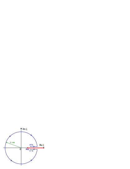
Figure 1: The integration contour in the complex $\zeta$–plane in Eq. (6). The physical cut $\zeta\geq 4m_{\pi}^{2}$ of the Adler function $D(-\zeta)$ (4) is shown along the positive semiaxis of real $\zeta$.

For practical purposes it proves to be convenient to deal with the Adler function [28]

$$D(Q^{2})=-\frac{d\,\Pi(-Q^{2})}{d\ln Q^{2}},$$ (4)

where $Q^{2}=-q^{2}>0$ denotes the spacelike kinematic variable. The corresponding dispersion relation [28]

$$D(Q^{2})=Q^{2}\int\limits_{4m_{\pi}^{2}}^{\infty}\frac{R(\sigma)}{(\sigma+Q^{2})^{2}}\,d\sigma$$ (5)

directly follows from Eqs. (2) and (4) and enables one to extract the experimental prediction for the Adler function from the respective measurements of the $R$–ratio. In turn, the theoretical expression for the function $R(s)$ can be obtained by integrating Eq. (4) in finite limits, namely [21, 22]

$$R(s)=\frac{1}{2\pi i}\lim_{\varepsilon\to 0_{+}}\int\limits_{s+i\varepsilon}^{s-i\varepsilon}D(-\zeta)\,\frac{d\zeta}{\zeta},$$ (6)

where the integration contour lies in the region of analyticity of the integrand, see Fig. 1. In particular, Eq. (6) relates the $R$–ratio to the Adler function, thereby providing a native way to properly account for all the effects due to continuation of the spacelike theoretical results into the timelike domain. At the same time, Eq. (4) additionally supplies the relation, which expresses the hadronic vacuum polarization function in terms of the Adler function, specifically [30]

$$\Delta\Pi(-Q^{2}\!,\,-Q_{0}^{2})=-\int\limits_{Q_{0}^{2}}^{Q^{2}}D(\zeta)\frac{d\zeta}{\zeta},$$ (7)

where $Q^{2}>0$ and $Q_{0}^{2}>0$ denote, respectively, the spacelike kinematic variable and the subtraction point.

In fact, Eqs. (2)–(7) form the complete set of relations, which mutually express the functions $\Pi(q^{2})$, $R(s)$, and $D(Q^{2})$ in terms of each other, and their derivation, being based only on the kinematics of the process on hand, requires neither additional approximations nor model–dependent phenomenological assumptions. In turn, the dispersion relations (2)–(7) impose a number of stringent physical nonperturbative restrictions on the functions $\Pi(q^{2})$, $R(s)$, and $D(Q^{2})$, that should certainly be accounted for when one reaches the limits of applicability of perturbative approach. It is worth mentioning also that the dispersively improved perturbation theory (DPT) [25, 31, 32, 33] (its preliminary formulation was discussed in Ref. [34]) conflates the foregoing nonperturbative constraints with corresponding perturbative input in a self–consistent way, thereby enabling one to overcome some inherent difficulties of the perturbative approach to QCD and extending its applicability range towards the infrared domain, see, in particular, Chaps. 4 and 5 of Ref. [25] and references therein for the details.

The nonperturbative aspects of the strong interactions will be disregarded in what follows and the rest of the paper will be primarily focused on the theoretical description of the $R$–ratio of electron–positron annihilation into hadrons at intermediate and high energies, that, in turn, allows one to safely neglect the effects due to the masses of the involved particles. At the same time, one has to be aware that in the limit of $m_{\pi}=0$ some of the aforementioned nonperturbative restrictions on the functions $\Pi(q^{2})$, $R(s)$, and $D(Q^{2})$, which play a substantial role at low energies, appear to be lost (a discussion of the effects due to the nonvanishing hadronic production threshold on the infrared behavior of the functions on hand can be found in Refs. [25, 31, 32, 33, 34, 35]).

2.2 Perturbative expressions for $\Pi(q^{2})$ and $D(Q^{2})$

In the framework of perturbation theory the hadronic vacuum polarization function (1) can be represented as

$$\Pi^{(\ell)}\bigl{(}q^{2},\mu^{2},a_{\text{s}}\bigr{)}=\sum_{j=0}^{\ell}\Bigl{[}a^{(\ell)}_{\text{s}}(\mu^{2})\Bigr{]}^{j}\sum_{k=0}^{j+1}\Pi_{j,k}\,\ln^{k}\!\!\left(\frac{\mu^{2}}{-q^{2}}\right)\!,\qquad q^{2}\to-\infty.$$ (8)

In this equation $\ell$ denotes the loop level, $q^{2}<0$ stands for the spacelike kinematic variable, $\mu^{2}>0$ is the renormalization scale, $a^{(\ell)}_{\text{s}}(\mu^{2})=\alpha^{(\ell)}_{\text{s}}(\mu^{2})\beta_{0}/(4\pi)$ denotes the so–called QCD couplant, $\beta_{0}=11-2n_{f}/3$ is the one–loop $\beta$ function perturbative expansion coefficient, $n_{f}$ stands for the number of active flavors, the common prefactor $N_{\text{c}}\sum_{f=1}^{n_{f}}Q_{f}^{2}$ is omitted throughout, $N_{\text{c}}=3$ denotes the number of colors, and $Q_{f}$ stands for the electric charge of $f$–th quark. The hadronic vacuum polarization function (8) satisfies the renormalization group equation

$$\left[\frac{\partial}{\partial\ln\mu^{2}}+\frac{\partial a_{\text{s}}(\mu^{2})}{\partial\ln\mu^{2}}\frac{\partial}{\partial a_{\text{s}}}\right]\!\Pi\bigl{(}q^{2},\mu^{2},a_{\text{s}}\bigr{)}=\gamma\bigl{(}a_{\text{s}}\bigr{)},$$ (9)

with $\gamma\bigl{(}a_{\text{s}}\bigr{)}$ being the corresponding anomalous dimension. At the $\ell$–loop level the perturbative expression for the latter takes the following form

$$\gamma^{(\ell)}\bigl{(}a_{\text{s}}\bigr{)}=\sum_{j=0}^{\ell}\gamma_{j}\Bigl{[}a^{(\ell)}_{\text{s}}(\mu^{2})\Bigr{]}^{j}.$$ (10)

Recall that at any given order $j\geq 1$ the perturbative coefficients $\Pi_{j,k}$ $(k=1,\ldots,j+1)$ entering Eq. (8) can be expressed in terms of the coefficients $\gamma_{i}$ $(i=1,\ldots,j)$ and (if $j\geq 2$) $\Pi_{i,0}$ $(i=1,\ldots,j-1)$ by making use of Eq. (9), see, e.g., Ref. [36] and references therein. Specifically, since the renormalization group equation for the $\ell$–loop perturbative QCD couplant $a^{(\ell)}_{\text{s}}(\mu^{2})$ reads

$$\frac{\partial a^{(\ell)}_{\text{s}}(\mu^{2})}{\partial\ln\mu^{2}}=-\sum_{i=0}^{\ell-1}B_{i}\Bigl{[}a^{(\ell)}_{\text{s}}(\mu^{2})\Bigr{]}^{i+2},\qquad B_{i}=\frac{\beta_{i}}{\beta_{0}^{i+1}},$$ (11)

Eq. (9) can be represented as

$$\sum_{j=0}^{\ell}\Bigl{[}a^{(\ell)}_{\text{s}}(\mu^{2})\Bigr{]}^{j}\!\left\{\!\left[\sum_{k=0}^{j+1}k\Pi_{j,k}\ln^{k-1}\!\!\left(\frac{\mu^{2}}{-q^{2}}\right)\!\right]\!-\gamma_{j}\right\}=$$

$$=\left\{\sum_{j=0}^{\ell}j\Bigl{[}a^{(\ell)}_{\text{s}}(\mu^{2})\Bigr{]}^{j-1}\sum_{k=0}^{j+1}\Pi_{j,k}\ln^{k}\!\!\left(\frac{\mu^{2}}{-q^{2}}\right)\!\!\right\}\left\{\sum_{i=0}^{\ell-1}B_{i}\Bigl{[}a^{(\ell)}_{\text{s}}(\mu^{2})\Bigr{]}^{i+2}\right\}\!.$$ (12)

In particular, at the first few loop levels Eq. (2.2) yields $\Pi_{0,1}=\gamma_{0}$, $\Pi_{1,1}=\gamma_{1}$, $\Pi_{2,1}=\Pi_{1,0}+\gamma_{2}$, $\Pi_{2,2}=\gamma_{1}/2$ ($\Pi_{j,j+1}=0$ for $j\geq 1$), see also Ref. [36]. At the higher loop levels the corresponding relations for the coefficients $\Pi_{j,k}$ (8), which will be needed for the purposes of Sect. 3.2, become rather cumbrous and are gathered in Appendix A.

As mentioned earlier, in practice it is convenient to employ the Adler function (4), which is defined as the logarithmic derivative of the hadronic vacuum polarization function (1). Specifically, Eq. (8) implies that at the $\ell$–loop level the perturbative expression for the Adler function (4) reads

$$D^{(\ell)}\bigl{(}Q^{2},\mu^{2},a_{\text{s}}\bigr{)}=\sum_{j=0}^{\ell}\Bigl{[}a^{(\ell)}_{\text{s}}(\mu^{2})\Bigr{]}^{j}\sum_{k=0}^{j+1}k\Pi_{j,k}\,\ln^{k-1}\!\!\left(\frac{\mu^{2}}{Q^{2}}\right)\!,\qquad Q^{2}\to\infty.$$ (13)

Then, the native choice of the renormalization scale $\mu^{2}=Q^{2}$ casts Eq. (13) to a well–known form ($\Pi_{0,1}=1$)

$$D^{(\ell)}(Q^{2})=\sum_{j=0}^{\ell}\Pi_{j,1}\Bigl{[}a^{(\ell)}_{\text{s}}(Q^{2})\Bigr{]}^{j}=1+d^{(\ell)}(Q^{2}),$$ (14)

where

$$d^{(\ell)}(Q^{2})=\sum_{j=1}^{\ell}d_{j}\Bigl{[}a^{(\ell)}_{\text{s}}(Q^{2})\Bigr{]}^{j}\!,\qquad d_{j}=\Pi_{j,1}$$ (15)

stands for the $\ell$–loop strong correction. For example, at the one–loop level ($\ell=1$) the Adler function (14) takes a quite simple form

$$D^{(1)}(Q^{2})=1+d_{1}a^{(1)}_{\text{s}}(Q^{2}),\qquad a^{(1)}_{\text{s}}(Q^{2})=\frac{1}{\ln(Q^{2}/\Lambda^{2})},$$ (16)

where $d_{1}=4/\beta_{0}$ and $\Lambda$ stands for the QCD scale parameter. As for the higher loop levels, the solution to the renormalization group equation for the QCD couplant (11) can be represented as the double sum

$$a^{(\ell)}_{\text{s}}(Q^{2})=\sum_{n=1}^{\ell}\sum_{m=0}^{n-1}b^{m}_{n}\,\frac{\ln^{m}(\ln z)}{\ln^{n}z},\qquad z=\frac{Q^{2}}{\Lambda^{2}},$$ (17)

where $b^{m}_{n}$ (the integer superscript $m$ is not to be confused with respective power) denotes the combination of the $\beta$ function perturbative expansion coefficients (in particular, $b^{0}_{1}=1$, $b^{0}_{2}=0$, $b^{1}_{2}=-\beta_{1}/\beta_{0}^{2}=-B_{1}$, see, e.g., Appendix A of Ref. [25]). Hence, the $\ell$–loop strong correction to the Adler function (15) can also be represented as

$$d^{(\ell)}(Q^{2})=\!\!\sum_{j=1}^{\ell}\!d_{j}\!\sum_{n_{1}=1}^{\ell}\ldots\sum_{n_{j}=1}^{\ell}\sum_{m_{1}=0}^{n_{1}-1}\ldots\sum_{m_{j}=0}^{n_{j}-1}\!\left(\prod_{i=1}^{j}b^{m_{i}}_{n_{i}}\right)\!\frac{\ln^{m_{1}+\ldots+m_{j}}(\ln z)}{\ln^{n_{1}+\ldots+n_{j}}z},$$ (18)

that appears to be technically more appropriate for the purposes of Sect. 3.1.

2.3 Various ways to handle $R(s)$

As outlined in Sect. 2.1, the $R$–ratio of electron–positron annihilation into hadrons can be calculated by making use of relation (6). In the massless limit one can cast the latter to (see also Ref. [37])

$$R^{(\ell)}(s)=1+r^{(\ell)}(s),\qquad r^{(\ell)}(s)=\int\limits_{s}^{\infty}\!\rho^{(\ell)}(\sigma)\,\frac{d\sigma}{\sigma}.$$ (19)

In this equation

$$\rho^{(\ell)}(\sigma)=\frac{1}{2\pi i}\lim_{\varepsilon\to 0_{+}}\Bigl{[}d^{(\ell)}(-\sigma-i\varepsilon)-d^{(\ell)}(-\sigma+i\varepsilon)\Bigr{]}$$ (20)

is the corresponding spectral function and $d^{(\ell)}(Q^{2})$ stands for the $\ell$–loop strong correction to the Adler function (15). As noted earlier, only perturbative contributions are retained in Eq. (20) herein, that, in turn, makes Eq. (19) identical to that of both the massless limit of the aforementioned DPT [25, 31, 32, 33] and the analytic approach [37, 44] (some of its recent applications can be found in, e.g., Refs. [45, 46, 47, 48, 49, 50, 51, 52]). At the one–loop level ($\ell=1$) the perturbative spectral function $\rho^{(1)}(\sigma)$ can easily be calculated by making use of Eqs. (20) and (16), namely

$$\rho^{(1)}(\sigma)=\frac{d_{1}}{y^{2}+\pi^{2}},\qquad y=\ln\biggl{(}\!\frac{\sigma}{\Lambda^{2}}\!\biggr{)}.$$ (21)

In turn, its integration (19) leads to a well–known result for the function $R(s)$

$$R^{(1)}(s)=1+d_{1}a^{(1)}_{\text{\scriptsize{TL}}}(s),\qquad a^{(1)}_{\text{\scriptsize{TL}}}(s)=\frac{1}{2}-\frac{1}{\pi}\arctan\biggl{(}\frac{\ln w}{\pi}\biggr{)},$$ (22)

where $w=s/\Lambda^{2}$ and it is assumed that $\arctan(x)$ is a monotone nondecreasing function of its argument: $-\pi/2\leq\arctan(x)\leq\pi/2$ for $-\infty<x<\infty$. In Eq. (22) $a^{(1)}_{\text{\scriptsize{TL}}}(s)$ constitutes the one–loop couplant, which properly incorporates all the effects of continuation of the perturbative expression $a^{(1)}_{\text{s}}(Q^{2})$ (16) from spacelike to timelike domain. Beyond the one–loop level, though the spectral function (20) can still be calculated explicitly at few lowest orders of perturbation theory in a straightforward way (see, in particular, Refs. [39, 46]), its integration (19) can, in general, be performed by making use of the numerical methods only, see, e.g., Refs. [54, 55].

At the higher–loop levels the explicit calculation of the perturbative spectral function (20) represents a rather demanding task, that eventually forces one to either evaluate $\rho^{(\ell)}(\sigma)$ in Eq. (19) numerically (that, however, requires a lot of computation resources and becomes quite sophisticated as $\ell$ increases, thereby essentially slowing down the overall computation process), or resort to an approximate expression for the $R$–ratio. In particular, for the latter purpose one can apply the Taylor expansion to the spectral function $\rho^{(\ell)}(\sigma)$ (20) at large values of its argument, that ultimately casts Eq. (19) to (see Refs. [25, 26, 56] and references therein for the details)

$$R^{(\ell)}(s) =1+\sum_{j=1}^{\ell}d_{j}\Bigl{[}a^{(\ell)}_{{\rm s}}(|s|)\Bigr{]}^{j}-\sum_{j=1}^{\ell}d_{j}\sum_{n=1}^{\infty}\!\frac{(-1)^{n+1}\pi^{2n}}{(2n+1)!}\sum_{k_{1}=0}^{\ell-1}\!\ldots\!\sum_{k_{2n}=0}^{\ell-1}\!\!\left(\,\prod_{p=1}^{2n}B_{k_{p}}\!\right)\!\!\times$$

$$\times\!\!\left[\,\prod_{t=0}^{2n-1}\!\Bigl{(}j+t+k_{1}+k_{2}+\ldots+k_{t}\Bigr{)}\!\right]\!\!\Bigl{[}a^{(\ell)}_{{\rm s}}(|s|)\Bigr{]}^{j+2n+k_{1}+k_{2}+\ldots+k_{2n}},\qquad\frac{\sqrt{s}}{\Lambda}>\exp\biggl{(}\frac{\pi}{2}\biggr{)}.$$ (23)

The re–expanded $R$–ratio (2.3) constitutes the sum of naive continuation ($Q^{2}=|s|$) of the perturbative expression for the Adler function $D^{(\ell)}(Q^{2})$ (14) into the timelike domain (the first two terms on its right–hand side) and an infinite number of the so–called $\pi^{2}$–terms. As demonstrated in Refs. [25, 26], Eq. (2.3) can provide quite accurate approximation of the $R$–ratio (19) for $\sqrt{s}/\Lambda>\exp(\pi/2)\simeq 4.81$, but only if one retains sufficiently many expansion terms on its right–hand side. However, the re–expansion (2.3) is commonly truncated at a given order $\ell$, that yields

$$R^{(\ell)}_{{\rm appr}}(s)=1+r^{(\ell)}_{\text{appr}}(s),\qquad r^{(\ell)}_{{\rm appr}}(s)=\sum_{j=1}^{\ell}r_{j}\Bigl{[}a^{(\ell)}_{\text{s}}(|s|)\Bigr{]}^{j},\qquad r_{j}=d_{j}-\delta_{j},$$ (24)

where $d_{j}$ denote the Adler function perturbative expansion coefficients (15) and $\delta_{j}$ incorporate the contributions of the kept $\pi^{2}$–terms. Specifically, at the first two orders the coefficients $\delta_{j}$ (24) vanish (i.e., $\delta_{1}=0$ and $\delta_{2}=0$), whereas at the higher–loop levels [23, 24, 57, 25, 26]

$$\delta_{3}\!=\!\frac{\pi^{2}}{3}d_{1},\quad\delta_{4}\!=\!\frac{\pi^{2}}{3}\biggl{(}\frac{5}{2}d_{1}B_{1}+3d_{2}\!\biggr{)}\!,\quad\delta_{5}\!=\!\frac{\pi^{2}}{3}\biggl{[}\frac{3}{2}d_{1}\Bigl{(}B_{1}^{2}+2B_{2}\Bigr{)}\!+7d_{2}B_{1}+6d_{3}\biggr{]}\!-\frac{\pi^{4}}{5}d_{1},\,$$ (25)

$$\delta_{6}\!=\!\frac{\pi^{2}}{3}\biggl{[}\frac{7}{2}d_{1}\Bigl{(}B_{1}B_{2}+B_{3}\Bigr{)}+4d_{2}\Bigl{(}B_{1}^{2}+2B_{2}\Bigr{)}+\frac{27}{2}d_{3}B_{1}+10d_{4}\biggr{]}\!-\frac{\pi^{4}}{5}\!\left(\frac{77}{12}d_{1}B_{1}+5d_{2}\!\right)\!\!,$$ (26)

$$\delta_{7} \!=\!\frac{\pi^{2}}{3}\Biggl{[}4d_{1}\!\left(\!B_{1}B_{3}+\frac{1}{2}B_{2}^{2}+B_{4}\!\right)+9d_{2}\Bigl{(}B_{1}B_{2}+B_{3}\Bigr{)}+\frac{15}{2}d_{3}\Bigl{(}B_{1}^{2}+2B_{2}\Bigr{)}+$$

$$+22d_{4}B_{1}+15d_{5}\Biggr{]}\!-\frac{\pi^{4}}{5}\left[\frac{5}{6}d_{1}\Bigl{(}17B_{1}^{2}+12B_{2}\Bigr{)}+\frac{57}{2}d_{2}B_{1}+15d_{3}\right]\!+\frac{\pi^{6}}{7}d_{1},$$ (27)

$$\delta_{8} \!=\!\frac{\pi^{2}}{3}\Biggl{[}\frac{9}{2}d_{1}\Bigl{(}B_{1}B_{4}+B_{2}B_{3}+B_{5}\Bigr{)}+10d_{2}\!\left(\!B_{1}B_{3}+\frac{1}{2}B_{2}^{2}+B_{4}\!\right)+\frac{33}{2}d_{3}\Bigl{(}B_{1}B_{2}+B_{3}\Bigr{)}+$$

$$+12d_{4}\Bigl{(}B_{1}^{2}+2B_{2}\Bigr{)}+\frac{65}{2}d_{5}B_{1}+21d_{6}\Biggr{]}\!-\frac{\pi^{4}}{5}\Biggl{[}\frac{15}{8}d_{1}\Bigl{(}7B_{1}^{3}+22B_{1}B_{2}+8B_{3}\Bigr{)}+$$

$$+\frac{5}{12}d_{2}\Bigl{(}139B_{1}^{2}+96B_{2}\Bigr{)}+\frac{319}{4}d_{3}B_{1}+35d_{4}\Biggr{]}\!+\frac{\pi^{6}}{7}\left(\frac{223}{20}d_{1}B_{1}+7d_{2}\right)\!.$$ (28)

The higher–order coefficients $\delta_{j}$ (24) can be found in Appendix C of Ref. [25]. It is worthwhile to recall here that the calculation of discontinuity (3) of the expression (8) with subsequent assignment of the renormalization scale $\mu^{2}=|s|$ also leads to the result identical to Eq. (24), see Sect. 3.2 for a discussion of this issue.

At the same time, it is necessary to outline that the approximation of the $R$–ratio in the form of Eq. (24) has certain shortcomings, see, e.g., Refs. [20, 21, 22, 23, 24]. In particular, the expression (24) discards all the higher–order $\pi^{2}$–terms, though the latter, being not necessarily negligible due to a rather large values of the coefficients $\delta_{j}$, may produce a sizable effect even at high energies. Moreover, the approximation $R^{(\ell)}_{{\rm appr}}(s)$ (24) becomes quite inaccurate when $s$ approaches the lower bound of its validity range $\sqrt{s}/\Lambda>\exp(\pi/2)\simeq 4.81$ and its loop convergence is worse than that of the expression (19), see Refs. [20, 21, 22, 23, 24, 25, 26] and references therein for a detailed discussion of these issues.

It is worthwhile to mention also that the explicit expression for the perturbative spectral function $\rho^{(\ell)}(\sigma)$ (20) has recently been derived at an arbitrary loop level in Refs. [25, 26]. On the one hand, the obtained expression for $\rho^{(\ell)}(\sigma)$ drastically simplifies the computation of the $R$–ratio (19), but on the other hand it still requires one to apply the methods of numerical integration, that may in general be somewhat effortful.

3 Results and Discussion

3.1 Explicit form of the $R$–ratio

The explicit expression for the $R$–ratio of electron–positron annihilation into hadrons, which properly embodies all the effects of continuation of perturbative results from spacelike to timelike domain, can be obtained in the following way. Namely, for this purpose it is convenient to employ relation (7) and Eq. (14) and then set $Q^{2}=-s-i0_{+}$ and $Q_{0}^{2}=-s+i0_{+}$, that makes the former identical (up to a constant factor $2\pi i$) to the relation (6). Equivalently, one can also employ relation (7) and Eq. (14), then set $Q^{2}=-s-i0_{+}$ and take its imaginary part, that makes the former identical (up to a constant factor $\pi$) to the relation (3).

Specifically, at the one–loop level ($\ell=1$) it is straightforward to demonstrate that relation (7) and Eq. (16) lead to (see, e.g., Refs. [20, 30, 25, 33])

$$\Delta\Pi^{(1)}(-Q^{2},-Q_{0}^{2})=-\ln\!\biggl{(}\frac{Q^{2}}{Q_{0}^{2}}\biggr{)}-d_{1}\ln\!\Biggl{[}\frac{a^{(1)}_{\text{s}}(Q_{0}^{2})}{a^{(1)}_{\text{s}}(Q^{2})}\Biggr{]}\!,$$ (29)

where $d_{1}=4/\beta_{0}$ and $a^{(1)}_{\text{s}}(Q^{2})=1/\ln(Q^{2}/\Lambda^{2})$. Then, the explicit expression for the function $R(s)$ can be obtained from Eq. (29) by making use of relation (3), namely

$$R^{(1)}(s)=\frac{1}{\pi}\,{\rm Im}\!\lim_{\varepsilon\to 0_{+}}\!\Delta\Pi^{(1)}(s+i\varepsilon,-Q_{0}^{2})=1+d_{1}\biggl{[}\frac{1}{2}-\frac{1}{\pi}\arctan\biggl{(}\frac{\ln w}{\pi}\biggr{)}\!\biggr{]},\qquad w=\frac{s}{\Lambda^{2}},$$ (30)

that obviously coincides with the result (22) obtained earlier from relation (6) and Eq. (16).

As for the higher–loop levels, Eq. (14) implies that the right–hand side of relation (7) is composed of the terms of a form

$$-\int\limits_{Q_{0}^{2}}^{Q^{2}}\frac{\ln^{m}\bigl{[}\ln(\zeta/\Lambda^{2})\bigr{]}}{\ln^{n}(\zeta/\Lambda^{2})}\frac{d\zeta}{\zeta}=-\!\!\!\int\limits_{\ln(\ln z_{0})}^{\ln(\ln z)}\!\!\!e^{-x(n-1)}x^{m}dx,$$ (31)

where $z=Q^{2}/\Lambda^{2}$ and $z_{0}=Q_{0}^{2}/\Lambda^{2}$. Then, since (up to an insufficient integration constant)

$$-\!\!\int\!\!e^{-x(n-1)}x^{m}dx=\begin{cases}\displaystyle-\frac{x^{m+1}}{m+1},&\text{if $\,n=1$},\\[11.38109pt] \displaystyle\frac{\Gamma\bigl{[}m+1,\,x(n-1)\bigr{]}}{(n-1)^{m+1}},\quad&\text{if $\,n\geq 2$}\end{cases}$$ (32)

and

$$\Gamma(m,x)=(m-1)!\,e^{-x}e_{m-1}(x)=(m-1)!\,e^{-x}\sum_{k=0}^{m-1}\frac{x^{k}}{k!},$$ (33)

one can cast Eq. (31) to

$$-\int\limits_{Q_{0}^{2}}^{Q^{2}}\frac{\ln^{m}\bigl{[}\ln(\zeta/\Lambda^{2})\bigr{]}}{\ln^{n}(\zeta/\Lambda^{2})}\frac{d\zeta}{\zeta}=J(Q^{2},n,m)-J(Q_{0}^{2},n,m),$$ (34)

where

$$J(Q^{2},n,m)=\begin{cases}\displaystyle-\frac{\ln^{m+1}(\ln z)}{m+1},&\text{if $\,n=1$},\\[11.38109pt] \displaystyle\sum_{k=0}^{m}\frac{m!}{k!}(n-1)^{k-m-1}\,\frac{\ln^{k}(\ln z)}{\ln^{n-1}z},\quad&\text{if $\,n\geq 2$}.\end{cases}$$ (35)

In Eq. (32) $\Gamma(m,x)$ stands for the complementary (or “upper”) incomplete gamma function, whereas in Eq. (33) $e_{m}(x)$ denotes the exponential sum function, see Ref. [58]. Thus, at the $\ell$–loop level relation (7) and Eq. (14) yield

$$\Delta\Pi^{(\ell)}(-Q^{2},-Q_{0}^{2})=-\ln\!\left(\frac{Q^{2}}{Q_{0}^{2}}\right)+\Delta p^{(\ell)}(Q^{2},Q_{0}^{2}),$$ (36)

where

$$\Delta p^{(\ell)}(Q^{2},Q_{0}^{2})=\sum_{j=1}^{\ell}d_{j}\Bigl{[}p^{(\ell)}_{j}(Q^{2})-p^{(\ell)}_{j}(Q_{0}^{2})\Bigr{]},$$ (37)

$$p^{(\ell)}_{j}(Q^{2})=\sum_{n_{1}=1}^{\ell}\ldots\sum_{n_{j}=1}^{\ell}\sum_{m_{1}=0}^{n_{1}-1}\ldots\sum_{m_{j}=0}^{n_{j}-1}\Biggl{(}\prod_{i=1}^{j}b^{m_{i}}_{n_{i}}\Biggr{)}J\Biggl{(}\!Q^{2},\sum_{i=1}^{j}n_{i},\sum_{i=1}^{j}m_{i}\!\Biggr{)},$$ (38)

the coefficients $d_{j}$ and $b^{m}_{n}$ are specified in Eqs. (15) and (17), respectively, and the function $J(Q^{2},n,m)$ is defined in Eq. (35).

In turn, the obtained expression (36) implies that at the higher–loop levels the right–hand side of relation (3) is comprised of the terms of a form

$$\frac{1}{2\pi i}\lim_{\varepsilon\to 0_{+}}\Bigl{[}\bar{a}_{n}^{m}(-s-i\varepsilon)-\bar{a}_{n}^{m}(-s+i\varepsilon)\Bigr{]}\!=\frac{1}{\pi}\,{\rm Im}\!\lim_{\varepsilon\to 0_{+}}\!\bar{a}_{n}^{m}(-s-i\varepsilon)=V_{n}^{m}(s),$$ (39)

where

$$\bar{a}_{n}^{m}(Q^{2})=\frac{\ln^{m}(\ln z)}{\ln^{n}z},\qquad z=\frac{Q^{2}}{\Lambda^{2}}.$$ (40)

The function $V_{n}^{m}(s)$ appearing in Eq. (39) reads

$$V_{n}^{m}(s)=\begin{cases}0,\quad&\text{if $\,n=0\,$ and $\,m=0$},\\[3.55658pt] v_{0}^{m}(s),\quad&\text{if $\,n=0\,$ and $\,m\geq 1$},\\[3.55658pt] v_{n}^{0}(s),&\text{if $\,n\geq 1\,$ and $\,m=0$},\\[3.55658pt] v_{n}^{0}(s)u_{0}^{m}(s)+u_{n}^{0}(s)v_{0}^{m}(s),\quad&\text{if $\,n\geq 1\,$ and $\,m\geq 1$},\end{cases}$$ (41)

where

$$v_{0}^{m}(s) =\!\sum\limits_{k=0}^{K(m)}\!\binom{m}{2k+1}(-1)^{k+1}\pi^{2k}\Bigl{[}L_{1}(y)\Bigr{]}^{m-2k-1}\,\Bigl{[}L_{2}(y)\Bigr{]}^{2k+1},$$ (42)

$$v_{n}^{0}(s) =\frac{1}{(y^{2}+\pi^{2})^{n}}\sum_{k=0}^{K(n)}\!\binom{n}{2k+1}(-1)^{k}\pi^{2k}y^{n-2k-1},$$ (43)

$$u_{0}^{m}(s) =\!\sum\limits_{k=0}^{K(m+1)}\!\binom{m}{2k}(-1)^{k}\pi^{2k}\Bigl{[}L_{1}(y)\Bigr{]}^{m-2k}\,\Bigl{[}L_{2}(y)\Bigr{]}^{2k},$$ (44)

$$u_{n}^{0}(s) =\frac{1}{(y^{2}+\pi^{2})^{n}}\sum_{k=0}^{K(n+1)}\!\binom{n}{2k}(-1)^{k}\pi^{2k}y^{n-2k},$$ (45)

$$L_{1}(y)=\ln\!\sqrt{y^{2}+\pi^{2}},\qquad L_{2}(y)=\frac{1}{2}-\frac{1}{\pi}\arctan\biggl{(}\frac{y}{\pi}\biggr{)},$$ (46)

$$\binom{n}{m}=\frac{n!}{m!\,(n-m)!},\qquad K(n)=\frac{n-2}{2}+\frac{n\;\mbox{mod}\;2}{2},$$ (47)

$(n\;\mbox{mod}\;m)$ denotes the remainder on division of $n$ by $m$, and $y=\ln w=\ln(s/\Lambda^{2})$. The function $V_{n}^{m}(s)$ (41) constitutes the generalization of the function $v_{n}^{m}(s)$ specified in Refs. [25, 26] and the details of its derivation are quite similar to those given therein. It is worthwhile to note that in Eqs. (39), (41)–(45), and on the left–hand side of Eq. (40) the integer superscript $m$ is not to be confused with respective power. Thus, at the $\ell$–loop level relation (3) and Eq. (36) lead to the following expression for the $R$–ratio of electron–positron annihilation into hadrons:

$$R^{(\ell)}(s)=1+r^{(\ell)}(s),\qquad r^{(\ell)}(s)=\sum\limits_{j=1}^{\ell}d_{j}\,A^{(\ell)}_{{\rm TL},j}(s),$$ (48)

where $d_{j}$ stand for the Adler function perturbative expansion coefficients (15),

$$A^{(\ell)}_{{\rm TL},j}(s)=\sum_{n_{1}=1}^{\ell}\ldots\sum_{n_{j}=1}^{\ell}\sum_{m_{1}=0}^{n_{1}-1}\ldots\sum_{m_{j}=0}^{n_{j}-1}\Biggl{(}\prod_{i=1}^{j}b^{m_{i}}_{n_{i}}\Biggr{)}\mbox{\tiny$\,$}T\mbox{\tiny$\!$}\Biggl{(}\!s,\sum_{i=1}^{j}n_{i},\sum_{i=1}^{j}m_{i}\!\Biggr{)}$$ (49)

denotes the $\ell$–loop $j$–th order “timelike” effective expansion function (that constitutes the continuation of the $j$–th power of $\ell$–loop QCD couplant $\bigl{[}a^{(\ell)}_{\text{s}}(Q^{2})\bigr{]}^{j}$ into the timelike domain), the coefficients $b^{m}_{n}$ are specified in Eq. (17),

$$T(s,n,m)=\begin{cases}\displaystyle-V_{0}^{1}(s),&\text{if $\,n=1\,$ and $\,m=0$},\\[7.11317pt] \displaystyle\sum_{k=0}^{m}\frac{m!}{k!}(n-1)^{k-m-1}\,V_{n-1}^{k}(s),\quad&\text{if $\,n\geq 2$},\end{cases}$$ (50)

and the function $V_{n}^{m}(s)$ is defined in Eq. (41). The obtained explicit expression for the $R$–ratio (48)–(50) properly accounts for all the effects due to continuation of the spacelike perturbative results into the timelike domain and, being valid at an arbitrary loop level, can easily be employed in practical applications.

It is worthwhile to note also that Eq. (49) certainly coincides with all five explicit expressions for the function $A^{(\ell)}_{{\rm TL},j}(s)$ obtained thus far by making use of the method described in Sect. 2.3. Specifically, as mentioned earlier, the one–loop first–order ($\ell=1$, $j=1$) expansion function (49) is identical to Eq. (22), which was obtained for the first time in Ref. [53], namely

$$A^{(1)}_{{\rm TL},1}(s)=L_{2}(y)=a^{(1)}_{\text{\scriptsize{TL}}}(s)=\frac{1}{2}-\frac{1}{\pi}\arctan\biggl{(}\frac{y}{\pi}\biggr{)},$$ (51)

where $L_{2}(y)$ is defined in Eq. (46) and $y=\ln w=\ln(s/\Lambda^{2})$. In turn, the two–loop first–order ($\ell=2$, $j=1$) expansion function (49)

$$A^{(2)}_{{\rm TL},1}(s)=L_{2}(y)-\frac{B_{1}}{y^{2}+\pi^{2}}\biggl{[}1+L_{1}(y)-yL_{2}(y)\biggr{]}$$ (52)

and the two–loop second–order ($\ell=2$, $j=2$) expansion function (49)

$$A^{(2)}_{{\rm TL},2}(s) =\frac{1}{y^{2}+\pi^{2}}+\frac{B_{1}}{(y^{2}+\pi^{2})^{2}}\biggl{\{}L_{2}(y)(y^{2}-\pi^{2})-y\Bigl{[}1+2L_{1}(y)\Bigr{]}\!\biggr{\}}+$$

$$+\frac{2}{3}\frac{B_{1}^{2}}{(y^{2}+\pi^{2})^{3}}\Biggl{\{}\!(3y^{2}-\pi^{2})\biggl{[}\frac{1}{9}+\frac{1}{3}L_{1}(y)+\frac{1}{2}\Bigl{(}L_{1}^{2}(y)-\pi^{2}L_{2}^{2}(y)\!\Bigr{)}\!\biggr{]}-$$

$$-y\Bigl{(}y^{2}-3\pi^{2}\Bigr{)}L_{2}(y)\biggl{[}\frac{1}{3}+L_{1}(y)\biggr{]}\!\Biggr{\}}$$ (53)

coincide with the corresponding expressions obtained for the first time in Ref. [21] and Ref. [25], respectively. In Eqs. (52) and (3.1) $B_{1}=\beta_{1}/\beta_{0}^{2}$ and $L_{1}(y)$ is specified in Eq. (46). It is also straightforward to verify that the three–loop first–order ($\ell=3$, $j=1$) and the four–loop first–order ($\ell=4$, $j=1$) expansion functions (49) are identical to the corresponding expressions obtained for the first time in Ref. [26]. The explicit form of the other functions $A^{(\ell)}_{{\rm TL},j}(s)$ had remained hitherto unavailable. In particular, as noted above, the computation of the functions $A^{(\ell)}_{{\rm TL},j}(s)$ and the study of the $R$–ratio at the first five loop levels, which was performed in Ref. [26], employ the methods of numerical integration.

3.2 Discussion

In fact, the foregoing approximate expression for the $R$–ratio (24) can be obtained in several equivalent ways. Specifically, to derive $R_{{\rm appr}}(s)$ (24) one can apply the Taylor expansion to the proper expression for the function $R(s)$ at high energies, rearrange the expansion terms in the way described in, e.g., Sect. 6.2 of Ref. [25], and then truncate it at a given order. Alternatively, one can apply the Taylor expansion to the corresponding spectral function $\rho(\sigma)$ (20) at large values of its argument, perform term–by–term integration (19) of the result [that yields Eq. (2.3)], and then truncate it at a given order. Additionally, as mentioned earlier, the calculation of discontinuity (3) of the expression $\Pi(q^{2},\mu^{2},a_{\text{s}})$ (8) with subsequent assignment of the renormalization scale $\mu^{2}=|s|$ (that amounts to an incomplete RG summation in the timelike domain, see, e.g., Refs. [20, 30] and references therein for a discussion of this issue) also leads to the result identical to Eq. (24). In particular, relation (3) and Eq. (8) imply that the coefficients $\delta_{j}$ entering $R_{{\rm appr}}(s)$ (24) read

$$\delta_{1}=0,\qquad\delta_{2}=0,\qquad\delta_{j}=\sum_{k=1}^{K(j)}(-1)^{k+1}\pi^{2k}\Pi_{j,2k+1},\qquad j\geq 3,$$ (54)

with $K(j)$ being defined in Eq. (47). The identity of the coefficients $\delta_{j}$ (54) to the corresponding expressions (25)–(2.3) can be demonstrated by making use of the results presented in Appendix A. At the same time, as noted above, one has to be aware that the approximation $R_{{\rm appr}}(s)$ (24) becomes quite rough when the energy scale $s$ approaches the lower bound of its validity range $\sqrt{s}/\Lambda>\exp(\pi/2)\simeq 4.81$ and its loop convergence is worse than that of the proper expression for the $R$–ratio (48). Moreover, the $\pi^{2}$–terms ignored in the truncated re–expanded approximation $R_{{\rm appr}}(s)$ (24) may produce a considerable effect even at high energies due to a rapid growth of the higher–order coefficients $\delta_{j}$, see, e.g., Refs. [20, 21, 22, 23, 24, 25, 26] and references therein.

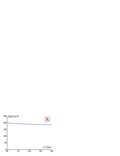
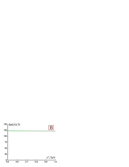
Figure 2: The relative difference (55) between the effect of inclusion of the $\pi^{2}$–terms discarded in the four–loop approximate expression $R^{(4)}_{{\rm appr}}(s)$ (24) and the effect of inclusion of the five–loop perturbative correction into Eq. (24) on the resulting value of the strong running coupling in $n_{f}=5$ energy range (plot A) and the future ILC experiment energy range [3] ($n_{f}=6$, plot B).

Specifically, to illustrate the convergence of the approximate form of the $R$–ratio (24), it is worth noting that at the four–loop level ($\ell=4$) at the scale of the $Z$ boson mass ($M_{{\rm Z}}=91.1876\,$GeV [60]) its third–order ($j=3$) and fourth–order ($j=4$) terms comprise, respectively, $34.2\,\%$ and $8.1\,\%$ of its second–order ($j=2$) term. As for the proper expression for the $R$–ratio (48), at the same loop level and energy scale its third–order ($j=3$) and fourth–order ($j=4$) terms comprise, respectively, only $1.8\,\%$ and $0.8\,\%$ of its second–order ($j=2$) term, thereby displaying much better convergence than that of Eq. (24). In particular, this exemplifies the fact that (as argued in Refs. [25, 26]) the $j$–th order contribution to the function $R(s)$ appears to be redistributed over the higher–order terms in its re–expansion (2.3). The reported findings also imply that the uncertainty of the resulting value of the strong running coupling associated with truncation of the proper expression for the $R$–ratio (48) at a given loop level is considerably less than that of its approximate form (24).

Additionally, Fig. 2 presents the relative difference between the impact of the higher–order $\pi^{2}$–terms omitted in the four–loop approximation $R^{(4)}_{{\rm appr}}(s)$ (24) and the impact of the five–loop perturbative correction to Eq. (24) on the evaluation of the strong running coupling. Namely, this figure displays the quantity

$$\Delta\alpha(|s|)=\left|\frac{\bar{\alpha}^{(4)}_{\text{s}}(|s|)-\alpha^{(4)}_{\text{s}}(|s|)}{\bar{\alpha}^{(4)}_{\text{s}}(|s|)-\bar{\alpha}^{(5)}_{\text{s}}(|s|)}\right|\!\times 100\%,$$ (55)

where $\alpha^{(\ell)}_{\text{s}}(|s|)$ and $\bar{\alpha}^{(\ell)}_{\text{s}}(|s|)$ stand for the $\ell$–loop strong running coupling evaluated at the energy scale $|s|$ by making use of, respectively, the proper expression $R^{(\ell)}(s)$ (48) and its approximate form $R^{(\ell)}_{{\rm appr}}(s)$ (24). In particular, as one can infer from Fig. 2, the effect of inclusion of the $\pi^{2}$–terms ignored in the four–loop approximate expression $R^{(4)}_{{\rm appr}}(s)$ (24) on the resulting value of the strong running coupling (likewise a similar impact on the $R$–ratio itself, see Refs. [25, 26]) is either prevailing over or comparable to the effect of inclusion of the five–loop perturbative correction into Eq. (24) even at high energies. Specifically, the former effect exceeds the latter one by a factor of two in $n_{f}=5$ energy range (plot A) and by a factor of $1.2$ in the energy range planned for the future ILC experiment [3] ($n_{f}=6$, plot B).

Table 1: The values of the strong running coupling and the QCD scale parameter at the first five loop levels $(\ell=1,\ldots,5)$ extracted from the mean value of the experimental data $R(s_{0})=1.18$ [61] by making use of the proper expression for the $R$–ratio (48) $\bigl{[}\alpha^{(\ell)}_{\text{s}}(|s_{0}|),\,\Lambda^{\!(\ell)}\bigr{]}$ and its approximate form (24) $\bigl{[}\bar{\alpha}^{(\ell)}_{\text{s}}(|s_{0}|),\,\bar{\Lambda}^{\!(\ell)}\bigr{]}$ at the energy scale of $\sqrt{s_{0}}=2\,$GeV.

	$\ell=1$	$\ell=2$	$\ell=3$	$\ell=4$	$\ell=5$
$\alpha^{(\ell)}_{\text{s}}(|s_{0}|)$	0.3283	0.3168	0.2955	0.2955	0.2924
$\Lambda^{\!(\ell)}$(MeV)	238	417	336	331	331
$\bar{\alpha}^{(\ell)}_{\text{s}}(|s_{0}|)$	0.2827	0.2501	0.2655	0.2881	0.3278
$\bar{\Lambda}^{\!(\ell)}$(MeV)	169	263	269	315	408

To elucidate the impact of the higher–order $\pi^{2}$–terms, discarded in the approximate expression for the $R$–ratio (24), on the evaluation of the strong running coupling itself, it is worthwhile to note the following. At the energy scale of $\sqrt{s_{0}}=2\,$GeV the four–loop strong running coupling assumes the value $\alpha^{(4)}_{\text{s}}(|s_{0}|)=0.2960\pm 0.0080$, the world average of the QCD scale parameter $\Lambda^{\!(4)}=(332\pm 17)\,$MeV [60] being employed. At the same time, the values of the strong running coupling and the QCD scale parameter at the first five loop levels $(\ell=1,\ldots,5)$ extracted from the corresponding mean value of the experimental data $R(s_{0})=1.18$ [61] are presented in Tab. 1. As earlier, the quantities $\bigl{[}\alpha^{(\ell)}_{\text{s}}(|s_{0}|),\,\Lambda^{\!(\ell)}\bigr{]}$ and $\bigl{[}\bar{\alpha}^{(\ell)}_{\text{s}}(|s_{0}|),\,\bar{\Lambda}^{\!(\ell)}\bigr{]}$ are evaluated by making use of the proper expression for the $R$–ratio (48) and its approximate form (24), respectively. As one can infer from Tab. 1, starting from the three–loop level ($\ell\geq 3$) the inclusion of the higher–order perturbative corrections into the proper expression for the $R$–ratio (48) yields a rather mild variation of the resulting values of the strong running coupling and the QCD scale parameter, thereby reflecting the aforementioned enhanced convergence of $R(s)$ (48). On the contrary, the use of an approximate form of the $R$–ratio (24) results in the values of $\bar{\alpha}^{(\ell)}_{\text{s}}(|s_{0}|)$ and $\bar{\Lambda}^{\!(\ell)}$, which show no sign of convergence and swerve away from the corresponding values of $\alpha^{(\ell)}_{\text{s}}(|s_{0}|)$ and $\Lambda^{\!(\ell)}$. In turn, this clearly demonstrates the fact that the approximation (24) is rather rough at the energy scale on hand and the higher–order $\pi^{2}$–terms omitted in $R^{(\ell)}_{{\rm appr}}(s)$ (24) play a significant role in the evaluation of the strong running coupling and the QCD scale parameter.

4 Conclusions

The explicit expression for the $R$–ratio of electron–positron annihilation into hadrons, which properly accounts for all the effects due to continuation of the spacelike perturbative results into the timelike domain, is obtained at an arbitrary loop level [Eqs. (48)–(50)]. Several equivalent ways to derive a commonly employed approximation of the $R$–ratio are recapped and the impact of the discarded in the latter higher–order $\pi^{2}$–terms on the evaluation of the strong running coupling is elucidated. The obtained results substantially facilitate the theoretical study of electron–positron annihilation into hadrons and the related strong interaction processes.

Acknowledgements

The author is grateful to Prof. A.B. Arbuzov for the stimulating discussions and useful comments.

Appendix A RG relations for the coefficients $\Pi_{j,k}$

As noted in Sect. 2.2, at any given order $j$ the hadronic vacuum polarization function perturbative expansion coefficients $\Pi_{j,k}$ $(k=1,\ldots,j+1)$ entering Eq. (8) can be expressed in terms of the coefficients $\gamma_{i}$ $(i=0,\ldots,j)$ appearing in Eq. (10) and (if $j\geq 2$) $\Pi_{i,0}$ $(i=1,\ldots,j-1)$ by making use of the renormalization group equation (9). The corresponding relations for the coefficients $\Pi_{j,k}$ at the first eight loop levels $(j=0,\ldots,8)$, which are needed for the purposes of Sect. 3.2, are presented in the following.

First of all, for $j=0$

$$\Pi_{0,1}=\gamma_{0}.$$ (56)

Then, for $j\geq 1$

$$\Pi_{j,j}=\frac{1}{j}\gamma_{1},\qquad\Pi_{j,j+1}=0.$$ (57)

In turn, for $j\geq 2$

$$\Pi_{j,1}=\gamma_{j}+\sum_{k=1}^{j-1}k\,\Pi_{k,0}\,B_{j-k-1},\qquad B_{j}=\frac{\beta_{j}}{\beta_{0}^{j+1}}.$$ (58)

For $j\geq 3$

$$\Pi_{j,2}=\Gamma_{j-1}+\!\sum_{k=1}^{j-2}k(j+k)\Pi_{k,0}\mathfrak{B}_{j-k-2},$$ (59)

where

$$\Gamma_{j}=\frac{1}{2}\sum_{k=1}^{j}k\gamma_{k}\,B_{j-k},\qquad\mathfrak{B}_{j}=\frac{1}{4}\sum_{k=0}^{j}B_{k}B_{j-k}.$$ (60)

For $j\geq 4$

$$\Pi_{j,3}=\frac{1}{3}\sum_{k=1}^{j-2}k(j+k)\Pi_{k,1}\mathfrak{B}_{j-k-2}.$$ (61)

The rest of the relations are given below:

$$\Pi_{5,4}=\Pi_{1,0}+\frac{13}{12}\gamma_{1}B_{1}+\gamma_{2}.$$ (62)

$$\Pi_{6,4} =\frac{77}{12}\Pi_{1,0}B_{1}+5\Pi_{2,0}+\gamma_{1}\biggl{(}\frac{35}{24}B_{1}^{2}+\frac{3}{2}B_{2}\!\biggr{)}\!+\frac{47}{12}\gamma_{2}B_{1}+\frac{5}{2}\gamma_{3},$$ (63)

$$\Pi_{6,5} =\Pi_{1,0}+\frac{77}{60}\gamma_{1}B_{1}+\gamma_{2}.$$ (64)

$$\Pi_{7,4} =\Pi_{1,0}\biggl{(}\frac{85}{6}B_{1}^{2}+10B_{2}\!\biggr{)}+\frac{57}{2}\Pi_{2,0}B_{1}+15\Pi_{3,0}+$$

$$+\gamma_{1}\biggl{(}\frac{5}{8}B_{1}^{3}+\frac{23}{6}B_{1}B_{2}+2B_{3}\!\biggr{)}+\gamma_{2}\biggl{(}\frac{59}{12}B_{1}^{2}+5B_{2}\!\biggr{)}+\frac{37}{4}\gamma_{3}B_{1}+5\gamma_{4},$$ (65)

$$\Pi_{7,5} =\frac{87}{10}\Pi_{1,0}B_{1}+6\Pi_{2,0}+\gamma_{1}\biggl{(}\frac{17}{6}B_{1}^{2}+2B_{2}\!\biggr{)}+\frac{57}{10}\gamma_{2}B_{1}+3\gamma_{3},$$ (66)

$$\Pi_{7,6} =\Pi_{1,0}+\frac{29}{20}\gamma_{1}B_{1}+\gamma_{2}.$$ (67)

$$\Pi_{8,4} =\Pi_{1,0}\biggl{(}\!\frac{105}{8}B_{1}^{3}+\frac{165}{4}B_{1}B_{2}+15B_{3}\!\biggr{)}\!\!+\Pi_{2,0}\biggl{(}\!\frac{695}{12}B_{1}^{2}+40B_{2}\!\biggr{)}\!\!+\frac{319}{4}\Pi_{3,0}B_{1}+35\Pi_{4,0}+$$

$$+\gamma_{1}\biggl{(}\frac{19}{8}B_{1}^{2}B_{2}+\frac{59}{12}B_{1}B_{3}+\frac{29}{12}B_{2}^{2}+\frac{31}{12}B_{4}\!\biggr{)}+\gamma_{2}\biggl{(}2B_{1}^{3}+\frac{73}{6}B_{1}B_{2}+\frac{25}{4}B_{3}\!\biggr{)}+$$

$$+\gamma_{3}\biggl{(}\frac{89}{8}B_{1}^{2}+\frac{45}{4}B_{2}\!\biggr{)}+\frac{107}{6}\gamma_{4}B_{1}+\frac{35}{4}\gamma_{5},$$ (68)

$$\Pi_{8,5} =\Pi_{1,0}\biggl{(}\frac{413}{15}B_{1}^{2}+15B_{2}\!\biggr{)}+\frac{459}{10}\Pi_{2,0}B_{1}+21\Pi_{3,0}+\gamma_{1}\biggl{(}\frac{21}{8}B_{1}^{3}+\frac{33}{4}B_{1}B_{2}+3B_{3}\!\biggr{)}+$$

$$+\gamma_{2}\biggl{(}\frac{139}{12}B_{1}^{2}+8B_{2}\!\biggr{)}+\frac{319}{20}\gamma_{3}B_{1}+7\gamma_{4},$$ (69)

$$\Pi_{8,6} =\frac{223}{20}\Pi_{1,0}B_{1}+7\Pi_{2,0}+\gamma_{1}\biggl{(}\frac{413}{90}B_{1}^{2}+\frac{5}{2}B_{2}\!\biggr{)}+\frac{153}{20}\gamma_{2}B_{1}+\frac{7}{2}\gamma_{3},$$ (70)

$$\Pi_{8,7} =\Pi_{1,0}+\frac{223}{140}\gamma_{1}B_{1}+\gamma_{2}.$$ (71)

References

- [1] FCC Collaboration, Eur. Phys. J. C 79, 474 (2019); Eur. Phys. J. ST 228, 261 (2019); 228, 755 (2019); report CERN–ACC–2018–0059 (2018); A. Blondel et al., arXiv:1906.02693 [hep-ph].
- [2] CEPC Study Group, arXiv:1809.00285 [physics.acc-ph]; arXiv:1811.10545 [hep-ex].
- [3] ILC Collaboration, arXiv:1306.6327 [physics.acc-ph]; arXiv:1306.6328 [physics.acc-ph]; arXiv:1306.6329 [physics.ins-det]; arXiv:1306.6352 [hep-ph]; arXiv:1306.6353 [physics.acc-ph].
- [4] CLICdp and CLIC Collaborations, CERN Yellow Rep. Monogr. Vol. 2 (2018); Vol. 3 (2018); Vol. 4 (2018); Vol. 1 (2019).
- [5] Muon g–2 Collaboration, arXiv:1501.06858 [physics.ins-det]; SciPost Phys. Proc. 1, 033 (2019).
- [6] E34 Collaboration, JPS Conf. Proc. 8, 025008 (2015); Y. Sato, PoS (KMI2017), 006 (2017); M. Abe et al., PTEP 5, 053C02 (2019).
- [7] C.M. Carloni Calame, M. Passera, L. Trentadue, and G. Venanzoni, Phys. Lett. B 746, 325 (2015); G. Abbiendi et al., Eur. Phys. J. C 77, 139 (2017); P. Mastrolia, M. Passera, A. Primo, and U. Schubert, JHEP 11, 198 (2017); S. Di Vita, S. Laporta, P. Mastrolia, A. Primo, and U. Schubert, ibid. 09, 016 (2018); M. Fael, ibid. 02, 027 (2019); M. Alacevich et al., ibid. 02, 155 (2019); G. Venanzoni, arXiv:1811.11466 [hep-ex]; U. Marconi, EPJ Web Conf. 212, 01003 (2019); G. Ballerini et al., Nucl. Instrum. Meth. A 936, 636 (2019); M. Fael and M. Passera, Phys. Rev. Lett. 122, 192001 (2019).
- [8] G.S. Bali, Phys. Rept. 343, 1 (2001); C. Gattringer and C.B. Lang, Lect. Notes Phys. 788, 1 (2010); P. Hagler, Phys. Rept. 490, 49 (2010); S. Aoki et al., Eur. Phys. J. C 77, 112 (2017); H.B. Meyer and H. Wittig, Prog. Part. Nucl. Phys. 104, 46 (2019).
- [9] M. Della Morte, B. Jaeger, A. Juttner, and H. Wittig, JHEP 03, 055 (2012); A. Francis, B. Jaeger, H.B. Meyer, and H. Wittig, Phys. Rev. D 88, 054502 (2013); M. Della Morte et al., JHEP 10, 020 (2017); C.A. Dominguez et al., Phys. Rev. D 96, 074016 (2017); A. Gerardin et al., arXiv:1904.03120 [hep-lat]; K. Miura, PoS (LATTICE 2018), 010 (2019).
- [10] C.D. Roberts, Prog. Part. Nucl. Phys. 61, 50 (2008); D. Binosi and J. Papavassiliou, Phys. Rept. 479, 1 (2009).
- [11] A.C. Aguilar, D. Binosi, and J. Papavassiliou, Phys. Rev. D 78, 025010 (2008); 86, 014032 (2012); 95, 034017 (2017); A.C. Aguilar, D. Binosi, J. Papavassiliou, and J. Rodriguez–Quintero, ibid. 80, 085018 (2009); A.C. Aguilar and J. Papavassiliou, ibid. 83, 014013 (2011); A.C. Aguilar, D. Ibanez, V. Mathieu, and J. Papavassiliou, ibid. 85, 014018 (2012); A.C. Aguilar, D. Binosi, D. Ibanez, and J. Papavassiliou, ibid. 90, 065027 (2014).
- [12] H.M. Fried, Modern functional Quantum Field Theory: summing Feynman graphs, Singapore, World Scientific, 266 p. (2014); H.M. Fried, Y. Gabellini, T. Grandou, and Y.-M. Sheu, Eur. Phys. J. C 65, 395 (2010); Annals Phys. 338, 107 (2013); H.M. Fried, T. Grandou, and Y.-M. Sheu, ibid. 327, 2666 (2012); 344, 78 (2014); H.M. Fried, P.H. Tsang, Y. Gabellini, T. Grandou, and Y.-M. Sheu, ibid. 359, 1 (2015).
- [13] U. Vogl and W. Weise, Prog. Part. Nucl. Phys. 27, 195 (1991); S.P. Klevansky, Rev. Mod. Phys. 64, 649 (1992); J. Bijnens, C. Bruno, and E. de Rafael, Nucl. Phys. B 390, 501 (1993); M. Buballa, Phys. Rept. 407, 205 (2005).
- [14] A.B. Arbuzov, E.A. Kuraev, and M.K. Volkov, Phys. Rev. C 82, 068201 (2010); 83, 048201 (2011); Eur. Phys. J. A 47, 103 (2011); M.K. Volkov, A.B. Arbuzov, and D.G. Kostunin, Phys. Rev. D 86, 057301 (2012); Phys. Rev. C 89, 015202 (2014); M.K. Volkov and A.B. Arbuzov, Phys. Part. Nucl. 47, 489 (2016); Phys. Usp. 60, 643 (2017).
- [15] A.E. Dorokhov and W. Broniowski, Eur. Phys. J. C 32, 79 (2003); Phys. Rev. D 78, 073011 (2008); A.E. Dorokhov, ibid. 70, 094011 (2004); A.E. Dorokhov, A.E. Radzhabov, and A.S. Zhevlakov, Eur. Phys. J. C 71, 1702 (2011); 72, 2227 (2012); 75, 417 (2015).
- [16] G. Colangelo, M. Hoferichter, A. Nyffeler, M. Passera, and P. Stoffer, Phys. Lett. B 735, 90 (2014); G. Colangelo, M. Hoferichter, B. Kubis, M. Procura, and P. Stoffer, ibid. 738, 6 (2014); G. Colangelo, M. Hoferichter, M. Procura, and P. Stoffer, JHEP 09, 091 (2014); 09, 074 (2015); 04, 161 (2017); Phys. Rev. Lett. 118, 232001 (2017); EPJ Web Conf. 175, 01025 (2018).
- [17] R. Garcia–Martin, R. Kaminski, J.R. Pelaez, and J. Ruiz de Elvira, Phys. Rev. Lett. 107, 072001 (2011); R. Garcia–Martin, R. Kaminski, J.R. Pelaez, J. Ruiz de Elvira, and F.J. Yndurain, Phys. Rev. D 83, 074004 (2011); S. Dubnicka, A.Z. Dubnickova, R. Kaminski, and A. Liptaj, ibid. 94, 054036 (2016); P. Bydzovsky, R. Kaminski, and V. Nazari, ibid. 94, 116013 (2016); E. Bartos, S. Dubnicka, A. Liptaj, A.Z. Dubnickova, and R. Kaminski, ibid. 96, 113004 (2017).
- [18] F. Guerrero and A. Pich, Phys. Lett. B 412, 382 (1997); A. Pich and J. Portoles, Phys. Rev. D 63, 093005 (2001); D. Gomez Dumm and P. Roig, Eur. Phys. J. C 73, 2528 (2013); P. Roig, A. Guevara, and G. Lopez Castro, Phys. Rev. D 89, 073016 (2014).
- [19] V. Bernard and E. Passemar, Phys. Lett. B 661, 95 (2008); V. Bernard, M. Oertel, E. Passemar, and J. Stern, Phys. Rev. D 80, 034034 (2009); G. Colangelo, E. Passemar, and P. Stoffer, Eur. Phys. J. C 75, 172 (2015); J. Phys. Conf. Ser. 800, 012026 (2017).
- [20] R.G. Moorhouse, M.R. Pennington, and G.G. Ross, Nucl. Phys. B 124, 285 (1977); M.R. Pennington and G.G. Ross, Phys. Lett. B 102, 167 (1981); M.R. Pennington, R.G. Roberts, and G.G. Ross, Nucl. Phys. B 242, 69 (1984).
- [21] A.V. Radyushkin, report JINR E2–82–159 (1982); JINR Rapid Commun. 78, 96 (1996); arXiv:hep-ph/9907228.
- [22] N.V. Krasnikov and A.A. Pivovarov, Phys. Lett. B 116, 168 (1982).
- [23] J.D. Bjorken, report SLAC–PUB–5103 (1989).
- [24] G.M. Prosperi, M. Raciti, and C. Simolo, Prog. Part. Nucl. Phys. 58, 387 (2007).
- [25] A.V. Nesterenko, Strong interactions in spacelike and timelike domains: Dispersive approach, Elsevier, Amsterdam, 222 p. (2017).
- [26] A.V. Nesterenko, Eur. Phys. J. C 77, 844 (2017).
- [27] R.P. Feynman, Photon–hadron interactions, Benjamin, Massachusetts, 282 p. (1972).
- [28] S.L. Adler, Phys. Rev. D 10, 3714 (1974).
- [29] T. Appelquist and H. Georgi, Phys. Rev. D 8, 4000 (1973).
- [30] A.A. Pivovarov, Nuovo Cim. A 105, 813 (1992).
- [31] A.V. Nesterenko and J. Papavassiliou, J. Phys. G 32, 1025 (2006).
- [32] A.V. Nesterenko, Phys. Rev. D 88, 056009 (2013).
- [33] A.V. Nesterenko, J. Phys. G 42, 085004 (2015).
- [34] A.V. Nesterenko and J. Papavassiliou, Phys. Rev. D 71, 016009 (2005); Int. J. Mod. Phys. A 20, 4622 (2005); Nucl. Phys. B (Proc. Suppl.) 152, 47 (2005); 164, 304 (2007).
- [35] A.V. Nesterenko, Nucl. Phys. B (Proc. Suppl.) 186, 207 (2009); 234, 199 (2013); Nucl. Part. Phys. Proc. 258, 177 (2015); 270, 206 (2016); SLAC eConf C0706044, 25 (2008); C1106064, 23 (2011); PoS (ConfinementX), 350 (2012); AIP Conf. Proc. 1701, 040016 (2016); EPJ Web Conf. 137, 05021 (2017).
- [36] P.A. Baikov, K.G. Chetyrkin, and J.H. Kuhn, Nucl. Phys. B (Proc. Suppl.) 189, 49 (2009); P.A. Baikov, K.G. Chetyrkin, J.H. Kuhn, and J. Rittinger, JHEP 07, 017 (2012).
- [37] K.A. Milton and I.L. Solovtsov, Phys. Rev. D 55, 5295 (1997); 59, 107701 (1999).
- [38] A.V. Nesterenko, Phys. Rev. D 62, 094028 (2000); 64, 116009 (2001).
- [39] A.V. Nesterenko, Int. J. Mod. Phys. A 18, 5475 (2003).
- [40] A.V. Nesterenko, Mod. Phys. Lett. A 15, 2401 (2000); A.V. Nesterenko and I.L. Solovtsov, ibid. 16, 2517 (2001); A.V. Nesterenko, Nucl. Phys. B (Proc. Suppl.) 133, 59 (2004).
- [41] A.C. Aguilar, A.V. Nesterenko, and J. Papavassiliou, J. Phys. G 31, 997 (2005); Nucl. Phys. B (Proc. Suppl.) 164, 300 (2007).
- [42] C. Contreras, G. Cvetic, O. Espinosa, and H.E. Martinez, Phys. Rev. D 82, 074005 (2010); C. Ayala, C. Contreras, and G. Cvetic, ibid. 85, 114043 (2012).
- [43] C. Ayala, G. Cvetic, and R. Kogerler, J. Phys. G 44, 075001 (2017); C. Ayala, G. Cvetic, R. Kogerler, and I. Kondrashuk, ibid. 45, 035001 (2018).
- [44] D.V. Shirkov and I.L. Solovtsov, Phys. Rev. Lett. 79, 1209 (1997); Theor. Math. Phys. 150, 132 (2007).
- [45] G. Cvetic and C. Villavicencio, Phys. Rev. D 86, 116001 (2012); C. Ayala and G. Cvetic, ibid. 87, 054008 (2013); P. Allendes, C. Ayala, and G. Cvetic, ibid. 89, 054016 (2014); C. Ayala, Nucl. Part. Phys. Proc. 294, 135 (2018); G. Cvetic, PoS (EPS–HEP2017), 367 (2017); Phys. Rev. D 99, 014028 (2019).
- [46] M. Baldicchi and G.M. Prosperi, Phys. Rev. D 66, 074008 (2002); AIP Conf. Proc. 756, 152 (2005); M. Baldicchi, G.M. Prosperi, and C. Simolo, ibid. 892, 340 (2007); M. Baldicchi, A.V. Nesterenko, G.M. Prosperi, and C. Simolo, Phys. Rev. D 77, 034013 (2008).
- [47] G. Cvetic and C. Valenzuela, Phys. Rev. D 74, 114030 (2006); 84, 019902(E) (2011); Braz. J. Phys. 38, 371 (2008); G. Cvetic and A.V. Kotikov, J. Phys. G 39, 065005 (2012).
- [48] G. Cvetic, A.Y. Illarionov, B.A. Kniehl, and A.V. Kotikov, Phys. Lett. B 679, 350 (2009); A.V. Kotikov, PoS (Baldin ISHEPP XXI), 033 (2013); PoS (Baldin ISHEPP XXII), 028 (2015); A.V. Kotikov, V.G. Krivokhizhin, and B.G. Shaikhatdenov, J. Phys. G 42, 095004 (2015); A.V. Kotikov, B.G. Shaikhatdenov, and P. Zhang, Phys. Rev. D 96, 114002 (2017); C. Ayala, G. Cvetic, A.V. Kotikov, and B.G. Shaikhatdenov, J. Phys. Conf. Ser. 938, 012055 (2017); Eur. Phys. J. C 78, 1002 (2018).
- [49] N. Christiansen, M. Haas, J.M. Pawlowski, and N. Strodthoff, Phys. Rev. Lett. 115, 112002 (2015); N. Mueller and J.M. Pawlowski, Phys. Rev. D 91, 116010 (2015); R. Lang, N. Kaiser, and W. Weise, Eur. Phys. J. A 51, 127 (2015); A. Dubla, S. Masciocchi, J.M. Pawlowski, B. Schenke, C. Shen, and J. Stachel, Nucl. Phys. A 979, 251 (2018).
- [50] K.A. Milton, I.L. Solovtsov, and O.P. Solovtsova, Phys. Lett. B 415, 104 (1997); 439, 421 (1998); Phys. Rev. D 60, 016001 (1999).
- [51] G. Ganbold, Phys. Rev. D 79, 034034 (2009); 81, 094008 (2010); Phys. Part. Nucl. 43, 79 (2012).
- [52] G. Cvetic, R. Kogerler, and C. Valenzuela, Phys. Rev. D 82, 114004 (2010); J. Phys. G 37, 075001 (2010); G. Cvetic and R. Kogerler, Phys. Rev. D 84, 056005 (2011).
- [53] B. Schrempp and F. Schrempp, Z. Phys. C 6, 7 (1980).
- [54] A.V. Nesterenko and C. Simolo, Comput. Phys. Commun. 181, 1769 (2010); 182, 2303 (2011).
- [55] C. Ayala and G. Cvetic, Comput. Phys. Commun. 190, 182 (2015); 199, 114 (2016); 222, 413 (2018).
- [56] A.V. Nesterenko and S.A. Popov, Nucl. Part. Phys. Proc. 282, 158 (2017).
- [57] A.L. Kataev and V.V. Starshenko, Mod. Phys. Lett. A 10, 235 (1995).
- [58] H. Bateman, Higher transcendental functions, Vols. I–III. McGraw–Hill, New York (1953).
- [59] P.A. Baikov, K.G. Chetyrkin, and J.H. Kuhn, Phys. Rev. Lett. 118, 082002 (2017); F. Herzog, B. Ruijl, T. Ueda, J.A.M. Vermaseren, and A. Vogt, JHEP 02, 090 (2017); T. Luthe, A. Maier, P. Marquard, and Y. Schroder, ibid. 10, 166 (2017).
- [60] M. Tanabashi et al. [Particle Data Group], Phys. Rev. D 98, 030001 (2018).
- [61] J.Z. Bai et al. [BES Collaboration], Phys. Rev. Lett. 88, 101802 (2002).