Fluctuation-dominated phase ordering at a mixed order transition

Abstract

Mixed order transitions are those which show a discontinuity of the order parameter as well as a divergent correlation length. We show that the behaviour of the order parameter correlation function along the transition line of mixed order transitions can change from normal critical behaviour with power law decay, to fluctuation-dominated phase ordering as a parameter is varied. The defining features of fluctuation-dominated order are anomalous fluctuations which remain large in the thermodynamic limit, and correlation functions which approach a finite value through a cusp singularity as the separation scaled by the system size approaches zero. We demonstrate that fluctuation-dominated order sets in along a portion of the transition line of an Ising model with truncated long-range interactions which was earlier shown to exhibit mixed order transitions, and also argue that this connection should hold more generally.

I Introduction

The locus which separates an ordered state from a disordered state with a diverging correlation length is usually characterized by power-law decays of correlation functions, indicative of critical behaviour. However, a growing number of systems show a related but distinct behaviour, termed fluctuation-dominated phase ordering (FDPO), along the critical line. (We continue to refer to the order-disorder separatrix as a critical line, even if the behaviour along it sometimes departs from traditional critical behaviour.) The crucial distinction is that in FDPO, the two-point correlation function of the order parameter $G(r|L)$ does not decay as a simple power, but rather is a scaling function of separation $r$ scaled by the system size $L$, in the limit $r\rightarrow\infty,L\rightarrow\infty$ with the ratio $\frac{r}{L}$ held constant; as this ratio approaches zero, the scaling function approaches a constant value in a singular fashion, through a cusp singularity:

$$G(r|L)\approx m_{0}^{2}-a\,\left|\frac{r}{L}\right|^{\alpha}+\cdots$$ (1)

where $m_{0}$ is the order parameter along the critical line, defined through the asymptotic behaviour of the two-point correlation function in an infinite system. The cusp exponent $\alpha$ lies between 0 and 1 and varies from system to system. This signature of FDPO has been found in several non-equilibrium models, ranging from particles on fluctuating surfaces DB ; DBM to active nematics MR ; DDR , granular collisions SDR and proteins on a cell surface DPR . A cusp in the correlation function also arises in disordered systems such as porous solids PZW , rough films AB1 and random-field Ising systems AB2 . The cusp singularity implies that the Porod Law ($\alpha=1$), familiar in the study of phase ordering dynamics AJB , does not hold; its breakdown is associated with the formation of anomalously large interfacial regions between ordered phases. The other principal characteristic of FDPO is the occurrence of very large fluctuations DBM ; DDR , leading to a broad distribution of the order parameter DBM ; KBB as well as some other observables DBM ; CB .

In this paper we explore the connection between FDPO and mixed order transitions (MOTs). These transitions are characterized by a discontinuity of the order parameter as in first order phase transitions together with a diverging correlation length as in second order transitions. Examples of mixed order transitions include some discrete spin models with long-range interactions DM1 ; DM2 ; DM3 ; DM4 ; DM5 , models of depinning transitions such as DNA denaturation PS ; MF and wetting transitions WT1 ; WT2 . More recent studies of glass and jamming transitions JT1 ; JT2 ; JT3 ; JT4 ; JT5 , evolution of complex networks CN1 ; CN2 ; CN3 ; CN4 and active polymer gels AP have shown that mixed order transitions take place in such systems as well. While all these systems do exhibit MOT, they differ in some of their features. In particular two broad classes of systems have been observed. In one class the correlation length diverges rather sharply, with essential singularity, as the transition is approached while in the other the divergence is algebraic. A prototypical model of the first class is the one- dimensional Ising model with ferromagnetic interactions decaying with distance $r$ as $r^{-2}$. It exhibits a Kosterlitz-Thouless (KT) vortex unbinding transition and it is dubbed IDSI for inverse distance squared Ising model. A paradigmatic model of the other class is the Poland-Scheraga model of DNA denaturation whereby the two strands of the DNA molecule separate from each other at a melting, or denaturation, temperature. It exhibits a condensation transition similar to the Bose Einstein condensation (BEC) transition of free bosons. In order to establish a link between these two classes of systems a modified version of the IDSI model has recently been introduced whereby the long-range interactions between the spins are restricted to exist only within domains of spins parallel to each other BM1 ; BM2 ; BMSM . This model is dubbed TIDSI for truncated inverse distance squared Ising model. The model is exacly soluble and it exhibits a mixed order transition of the second class with algebraically diverging correlation length. The transition separates a totally ordered, non-fluctuating ferromagnetic phase from a disordered phase. Specific properties of this model have been studied and characterized, including the partition function, the distributions of cluster sizes, and the distribution of the length of the longest cluster.

We show below that part of the critical line of the TIDSI exhibits FDPO, characterized by extensive fluctuations and a cusp in the scaled correlation function as in Eq. (1). A key parameter in the model is the ratio of the strength of the inverse squared interaction to the temperature, denoted by $c$. Recent work on the distribution of the length $l_{\rm max}$ of the largest domain in various phases of this model has revealed BMSM that along the critical line and for $1<c<2$, while a typical domain is subextensive, the maximal domain is extensive. Moreover, the exact form of the distribution BMSM of $l_{\rm max}$ on the critical line indicates the existence of large fluctuations for $1<c<2$. This naturally raises the possibility that on the critical line and for $1<c<2$, the TIDSI model may exhibit FDPO. One good test would be to see if the spin-spin correlation function also exhibits the signature of FDPO in this regime. In this paper, we calculate exactly the spin-spin correlation functions $G(r|L)$ for the TIDSI model and show that along the critical line, there is a change from normal critical behaviour $G(r)\approx A/r^{c-2}\text{~{}~{}as~{}~{}}\,r\rightarrow\infty$ for $c>2$, to a size-dependent scaling function with a cusp singularity in the region $1<c<2$. Our result thus demonstrates very clearly that indeed the region $1<c<2$ on the critical line exhibits FDPO.

The occurrence of FDPO in the TIDSI model brings out several interesting points. First, the TIDSI is an equilibrium system in contrast to the nonequilibrium systems studied in DB ; DBM ; KBB ; CB . It appears that the long-range interaction in the TIDSI model is the key element which induces FDPO, suggesting that FDPO may well occur in other settings where interactions are sufficiently long-ranged. Secondly, we find that the cusp exponent $\alpha$ varies continuously along the critical line, as a function of a parameter. Such a variation of the cusp exponent has not been observed in earlier studies of FDPO, within a single model. Thirdly, the onset of FDPO coincides with the point at which the maximal domain becomes extensive. This interesting correlation between FDPO and extreme value statistics has been observed before in the context of a coarse-grained depth (CD) model DBM ; CB which mimics particles sliding down fluctuating surfaces in the adiabatic limit. Lastly, our study brings into focus the general question of the relation between FDPO and MOTs, as there are several other examples of MOTs which are associated with FDPO.

The remainder of the paper is organized as follows. In Section II, we define the TIDSI model, and show that when domain sizes are large, for instance near the critical line, one may represent configurations in terms of domains. In Section III we compute the asymptotic behavior of the partition function and derive the phase diagram. The Section also contains the computation of the marginal domain size distribution in different regions of the phase boundary. Section IV discusses FDPO in the TIDSI model in terms of the two-point spin-spin correlation function. In the concluding Section IV, we discuss the issues set out in the previous paragraph, along with some open questions. Some details and an alternative derivation of the correlation function are presented in Appendix A.

II The Model and the Domain Representation

The TIDSI model is an Ising model defined on a one-dimensional lattice where on each site $i$ there is a spin variable $\sigma_{i}=\pm 1$. The interaction between spins is composed of a nearest neighbor term $-J_{NN}\sigma_{i}\sigma_{i+1}$ together with a long-range interaction term $-J(i-j)\sigma_{i}\sigma_{j}I(i\sim j)$, where $I(i\sim j)=1$ as long as sites $i$ and $j$ are in the same domain of either all up or all down spins and $I(i\sim j)=0$ otherwise. The long-range coupling is taken to be of the form

$$J(r)\approx\frac{C}{r^{2}}\quad\,\text{for}\,\,r\gg 1$$ (2)

The indicator function $I(i\sim j)$ may be expressed in terms of the spin variables

$$I(i\sim j)=\prod^{j-1}_{k=i}\delta_{\sigma_{k}\sigma_{k+1}}=\prod^{j-1}_{k=i}\frac{1+\sigma_{k}\sigma_{k+1}}{2}$$ (3)

The TIDSI Hamiltonian may thus be written as

$$\mathcal{H}=-J_{NN}\sum_{i=1}^{N}\sigma_{i}\sigma_{i+1}-\sum_{i<j}J(i-j)\sigma_{i}\sigma_{j}\prod^{j}_{k=i}\frac{1+\sigma_{k}\sigma_{k+1}}{2}$$ (4)

It is convenient to express the Hamiltonian in terms of the domain length representation, where a domain is defined as a stretch of successive parallel spins (see Fig. 1). This representation has been described in (BM2 ; BMSM ) but a brief account is included here for completeness. The long-range interaction in the second term operates only between pairs of spins which belong to the same domain, while the nearest neighbor interaction in the first term results in an energy cost for each domain wall. A typical configuration $\mathcal{C}$ is thus described by a set of domains with lengths $\{l_{1},\,l_{2},\,\cdots,\,l_{N}\}$ where the number of domains $N$ can vary from one configuration to another. The total system size $L$ and Hamiltonian can be expressed as

$$\sum^{N}_{n=1}l_{n}=L$$ (5)

$$\mathcal{H}=\sum^{N}_{n=1}\mathcal{H}_{n}-J_{NN}$$ (6)

where

$$\mathcal{H}_{n}=-J_{NN}(l_{n}-2)-\sum^{l_{n}}_{r=1}(l_{n}-r)J(r)$$ (7)

Using the form of $J(r)$ in Eq. (2), one can estimate the sum via replacing it by an integral as

$$\sum J(r) \approx a_{0}-\frac{C}{l_{n}}$$

$$\sum rJ(r) \approx b_{0}+C\,\ln(l_{n})\,,$$ (8)

where we have assumed $l_{n}$ is large and kept the two leading order terms for large $l_{n}$. This is justified since we are interested in phenomena close to the critical line where domains are typically large. Dropping an overall unimportant constant, one obtains an the effective Hamiltonian

$$\mathcal{H}=C\sum_{n}\ln(l_{n})+\Delta N$$ (9)

where the constant $C$ is the amplitude of the long-range interaction and $\Delta=2J_{NN}+C+b_{0}$ acts as a chemical potential for the number of domains. It is useful to define the parameter $c=\beta C$, as it enters in an important way in the subsequent development.

Figure 1: A typical configuration of the domains in the TIDSI model, where the number of domains $N=5$ with domain lengths $l_{1}$, $l_{2}$, $l_{3}$, $l_{4}$ and $l_{5}$. They satisfy the sum rule $\sum_{i=1}^{N}l_{i}=L$ with $L$ denoting the system size.

As mentioned before, a configuration $\mathcal{C}$ of the system is now specified by the domain sizes, as well as the number of domains $N$: $\mathcal{C}\equiv\{l_{1},\,l_{2},\,\cdots,\,l_{N},\,N\}$. The probability of such a configuration $\mathcal{C}$ is given by its Boltzmann weight

$$P(l_{1},\,l_{2},\,\cdots,\,l_{N},\,N|L)=\frac{y^{N}}{Z_{y}(L)}\,\prod^{N}_{n=1}\,\frac{1}{l_{n}^{c}}\,\delta_{\sum^{N}_{n=1}l_{n},\,L}$$ (10)

where $y=e^{-\beta\Delta}$ and $\delta_{i,j}$ is the Kronecker delta function that enforces the sum rule. The normalization constant $Z_{y}(L)$ is indeed the partition function given by

$$Z_{y}(L)=\sum^{\infty}_{N=1}y^{N}\sum^{\infty}_{l_{1}=1}\ldots\sum_{l_{N}=1}^{\infty}\prod^{N}_{n=1}\frac{1}{l_{n}^{c}}\,\,\,\delta_{\sum^{N}_{n=1}l_{n},\,L}\,.$$ (11)

As we will see below, the way in which $Z_{y}(L)$ scales with system size $L$ changes depending on the value of the two parameters $c$ and $y$. We will thus consider $c$ and $y$ as independent parameters and discuss the behaviour of the system in different regimes in the $(c-y)$ plane. Even though the joint distribution in Eq. (10) is well defined for any $c>0$, it turns out that for $0<c\leq 1$, there is no phase transition as a function of $y$ and the system is always in a paramagnetic phase. In contrast, for $c>1$, there is a phase transition in the $(c-y)$ plane across the critical line $y_{c}=1/\zeta(c)$ where $\zeta(c)=\sum_{l=1}^{\infty}l^{-c}$ is the Riemann zeta function. For $c>1$, the system is in a paramagnetic phase for $y>y_{c}$, while it is ferromagnetic for $y<y_{c}$ (see the phase diagram in Fig. (2)). Hence, in the rest of the paper, we will restrict ourselves to the case $c>1$.

III Partition function, phase diagram and domain size distribution

The partition function and the phase diagram of this model has been analysed before in the $(c-T)$ plane in Refs BM1 ; BM2 . In this section, we re-derive some of these results in the $(c-y)$ plane (the details are slightly different from those in the $(c-T)$ plane). Some of these results will be useful later for computing the marginal domain size distribution, as well as the spin-spin correlation function.

III.1 Partition function and phase diagram

To analyse the behaviour of the partition function $Z_{y}(L)$ in Eq. (11) in different regimes in the $(c-y)$ plane, let us define its generating function

$$\tilde{Z}_{y}(s)=\sum^{\infty}_{L=1}e^{-sL}Z_{y}(L)\,.$$ (12)

The generating function corresponding to Eq. (11) is

$$\tilde{Z}_{y}(s)=\sum^{\infty}_{L=1}e^{-sL}Z_{y}(L)=\frac{y\phi(s)}{1-y\phi(s)}$$ (13)

with

$$\phi(s)=\sum^{\infty}_{l=1}\frac{e^{-sl}}{l^{c}}={\rm Li}_{c}\left(e^{-s}\right)\,,$$ (14)

where ${\rm Li}_{c}(z)=\sum_{l=1}^{\infty}\frac{z^{l}}{l^{c}}$ is the polylogarithmic function. Thus, to extract the large $L$ asymptotic behavior of $Z_{y}(L)$, we need to analyse the singularities of the right hand side (rhs) of Eq. (13) as a function of $s$.

Clearly $\phi(s)$ in Eq. (14) decreases monotonically as $s$ increases from $0$ to $\infty$, starting from $\phi(0)=\zeta(c)$. Near $s=0$, using the known asymptotic behavior of polylogarithms, one can show that $\phi(s)$ has the asymptotic expansion

$$\phi(s)=\sum_{k=0}^{n-1}\frac{(-s)^{k}}{k!}\zeta(c-k)+\Gamma(1-c)\,s^{c-1}+\dots$$ (15)

where $n={\rm int}[c]$ (for integer $c$, the first non-analytic term gets additional multiplicative logarithmic corrections). In contrast, as $s\to\infty$, the leading behavior of $\phi(s)$ comes from the $l=1$ term in Eq. (14), implying $\phi(s)\approx e^{-s}$ for large $s$. Thus, as a function of $s$, the rhs of Eq. (13) has a pole at some $s=s^{*}>0$, provided $1/y<\phi(0)=\zeta(c)$. We will see later that this corresponds to the paramagnetic phase. As $y\to y_{c}=1/\zeta(c)$ from above, the pole $s^{*}\to 0$ and we need to analyse the rhs for small $s$ and we will see below that $y<y_{c}$ will correspond to the ferromagnetic phase. Below we analyse the large $L$ behavior of $Z_{y}(L)$ in the three regimes separately: (i) paramagnetic phase ($y>y_{c}$) (ii) critical point ($y=y_{c}$) and (iii) ferromagnetic phase ($y<y_{c}$).

Since the large $L$ behavior of $Z_{y}(L)$ corresponds to the small $s$ behavior of the generating function ${\tilde{Z}}_{y}(s)$, we first approximate, for small $s$, the sum in Eq. (12) by an integral, i.e., the generating function coincides with the Laplace transform

$$Z_{y}(s)\approx\int_{0}^{\infty}Z_{y}(L)\,e^{-sL}\,dL=\frac{y\phi(s)}{1-y\phi(s)}\,.$$ (16)

Inverting the Laplace transform, we can express $Z_{y}(L)$ as a Bromwich integral in the complex $s$ plane

$$Z_{y}(L)=\int_{\Gamma_{0}}\frac{ds}{2\pi i}\,e^{sL}\,\frac{y\phi(s)}{1-y\phi(s)}$$ (17)

where $\Gamma_{0}$ is a vertical contour whose real part is to the right of all singularities of the integrand in the complex $s$ plane. Below we analyse the large $L$ behavior of this Bromwich integral in the three regimes.

(i) Paramagnetic phase ($y>y_{c}$): In this case, the integrand in Eq. (17) has a pole at $s=s^{*}>0$, where $y\phi(s^{*})=1$. As argued above, this happens provided $y>y_{c}=1/\phi(0)=1/\zeta(c)$. In this case, the leading large $L$ behavior of the Bromwich integral comes from this pole $s^{*}$ in the $s$ plane. Evaluating the residue, we obtain

$$Z_{y}(L)\approx B_{0}\,e^{s^{*}L}\,;\quad{\rm where}\quad B_{0}=\frac{1}{-y\phi^{\prime}(s^{*})}$$ (18)

Thus the free energy $-\ln Z_{y}(L)\sim s^{*}L$ is extensive in $L$, clearly indicating that we are in a paramagnetic phase. As $y\to y_{c}$ from above, for fixed $c>1$, the pole $s^{*}\to 0$, and we need to analyse the nonanalytic behavior of the integrand near its branch cut at $s=0$.

(ii) Critical line ($y=y_{c}$): We set $y=y_{c}$ on the rhs of Eq. (16) and replace $\phi(s)$ by its small $s$ behavior in Eq. (15). For the leading $s$ behavior, in the numerator $y_{c}\phi(s)$ on the rhs in Eq. (16), we can just keep the leading term $\phi(s)=\zeta(c)$ (the higher order corrections lead to only subleading behavior). Hence $y\phi(s)\approx 1$. In contrast, using $y_{c}=1/\zeta(c)$, the leading term for small $s$ in the denominator depends crucially on whether $c>2$ or $1<c<2$.

• $c>2$: For $c>2$, the leading order term in the denominator of the rhs of Eq. (16) is the analytic term, $1-y_{c}\phi(s)\approx y_{c}\zeta(c-1)s$. Hence, $Z_{y}(s)\approx 1/[y_{c}\zeta(c-1)s]$, whose Laplace inversion gives trivially

  $$Z_{y}(L)\approx\frac{1}{y_{c}\zeta(c-1)}=\frac{\zeta(c)}{\zeta(c-1)}=B_{1}\,.$$ (19)

  Thus, the partition function approaches a constant $B_{1}$ as $L\to\infty$.

• $1<c<2$: In this case, the leading order term in the denominator of the rhs of Eq. (16) for small $s$ is the non-analytic term in the small $s$ expansion of $\phi(s)$ in Eq. (15), i.e., $1-y_{c}\phi(s)\approx-y_{c}\Gamma(1-c)\,s^{c-1}$. Hence, $Z_{y}(s)\approx-1/[y_{c}\Gamma(1-c)s^{c-1}]$ as $s\to 0$. Inverting the Laplace transform in a straightforward way and simplifying, we get

  $$Z_{y}(L)\approx B_{2}\,L^{c-2}\,;\quad{\rm where}\quad B_{2}=\frac{1}{\pi}\zeta(c)(c-1)\sin(\pi(c-1))\,.$$ (20)

  Thus, for $1<c<2$, the partition function decays algebraically for large $L$ as $L^{c-2}$.

(iii) Ferromagnetic phase ($y<y_{c}$): Finally, we turn to the ferromagnetic phase $y<y_{c}=1/\zeta(c)$. In this case, substituting the small $s$ behavior of $\phi(s)$ from Eq. (15) in the rhs of Eq. (16), we find the following leading small $s$ behavior for the Laplace transform

$$\int_{0}^{\infty}Z_{y}(L)\,e^{-sL}\,dL\approx\frac{y\zeta(c)}{1-y\zeta(c)}+``{\rm analytic\,\,terms}^{\prime\prime}+\frac{y\Gamma(1-c)}{(1-y\zeta(c))^{2}}\,s^{c-1}+\cdots$$ (21)

Note that the leading constant term is positive if and only if $y<y_{c}=1/\zeta(c)$, clearly indicating that this expansion makes sense only in the ferromagnetic phase. The leading nonanalytic term for small $s$ in the Laplace transform in Eq.(21) fixes the leading large $L$ behavior of $Z_{y}(L)$ uniquely via a Tauberian theorem and we get

$$Z_{y}(L)\approx B_{3}\,L^{-c}\,;\quad{\rm where}\quad B_{3}=\frac{y}{(1-y\zeta(c))^{2}}\,.$$ (22)

Thus, in the ferromagnetic phase, for any $c>1$, the partition function decays as $L^{-c}$ for large $L$.

Let us then just summarize the behavior of the partition function $Z_{y}(L)$ for large $L$ in the $(c-y)$ plane in Fig. (2):

$$Z_{y}(L)\approx\begin{cases}&B_{0}\,e^{s^{*}\,L}\quad{\rm for}\quad y>y_{c}=1/\zeta(c)\quad(\rm PARA)\\ &B_{1}\quad\quad\quad\,{\rm for}\quad y=y_{c}\,\,{\rm and}\,\,c>2\quad(\rm CRITICAL\,\,LINE)\\ &B_{2}\,L^{c-2}\quad{\rm for}\quad y=y_{c}\,\,{\rm and}\,\,1<c<2\quad(\rm CRITICAL\,\,LINE)\\ &B_{3}\,L^{-c}\quad\,\,{\rm for}\quad y<y_{c}=1/\zeta(c)\quad(\rm FERRO)\\ \end{cases}$$ (23)

where $s^{*}$ is the solution of $y\phi(s^{*})=1$ for $y>y_{c}$ and the four constants $B_{0}$, $B_{1}$, $B_{2}$ and $B_{3}$ are given respectively in Eqs. (18), (19), (20) and (22). This also leads to the phase diagram in Fig. (2). We emphasize that on the critical line $y=y_{c}$, the partition function behaves rather differently as a function of $L$ for $c>2$ and $1<c<2$ (shown respectively by the dashed line and the soild (red) line in the phase diagram in Fig. (2).

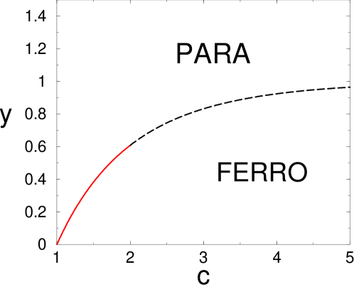
Figure 2: Phase diagram in the $(c-y)$ plane, where $c>1$. The critical line $y_{c}=1/\zeta(c)$ separates the paramagnetic phase ($y>y_{c}$) from the ferromagnetic phase ($y<y_{c}$). The system exhibits FDPO on the part $1<c\leq 2$ of the critical line (shown by the solid (red) line).

III.2 Distribution of the domain sizes

In this subsection, we compute the marginal domain size distribution $P_{y}(l|L)$, i.e., the probability that a randomly picked domain has size $l$, given the total system size $L$ and for fixed $c$ and $y$. This is done as follows. We start from the joint distribution of domain lengths and the number of domains in Eq. (10), keep one of the domain lengths fixed at $l$ (say $l_{1}=l$), and sum over all other $l_{i}$’s as well as $N$. This gives

$$P(l|L)=\frac{y}{l^{c}}\,\frac{1}{Z_{y}(L)}\,\sum_{N=1}^{\infty}\,\sum_{l_{2}\geq 1,\cdots,l_{N}\geq 1}\frac{y^{N-1}}{l_{2}^{c}\,l_{3}^{c}\cdots l_{N}^{c}}\,\delta_{l_{2}+l_{3}+\cdots+l_{N},L-l}\,.$$ (24)

Note that, using the partition function $Z_{y}(L)$ in Eq. (11), the marginal distribution satisfies, by construction, the normalization condition $\sum_{l\geq 1}P(l|L)=1$. Indeed, $P(l|L)$ can also be interpreted as follows: given that a domain wall occurs, $P(l|L)$ is the probability that the next domain wall to the right occurs at a distance $l$.

To proceed, we consider the sum over $N=1,2\cdots$ in Eq. (24), and separate the $N=1$ term (only one domain in the whole system) and $N\geq 2$ terms. The sum over $N\geq 2$ can be reexpressed in terms of the partition function $Z_{y}(L)$ in Eq. (11). This gives

$$P(l|L)=\frac{y}{L^{c}\,Z_{y}(L)}\,\delta_{l,\,L}+\frac{y}{l^{c}}\,\frac{Z_{y}(L-l)}{Z_{y}(L)}\,$$ (25)

where the first term corresponds to $N=1$. Note that Eq. (25) is exact for all $l\geq 1$ and $L\geq 1$. The next step is to analyse this marginal distribution $P(l|L)$ for large $L$ in different regions of the phase diagram in the $(c-y)$ plane in Fig. (2). For this, we will use the asymptotic properties of the partition function $Z_{y}(L)$ derived in the previous subsection that are summarized in Eq. (23).

(i) Paramagnetic phase ($y>y_{c}=1/\zeta(c)$): In this regime, $Z_{y}(L)\sim e^{s^{*}\,L}$ for large $L$ from Eq. (23), where $s^{*}>0$ is the root of $y\,\phi(s^{*})=1$ with $y>y_{c}$ (recall that $\phi(s)$ is given in Eq. (14)). The first term in Eq. (25), i.e., the delta peak behaves as $\approx\frac{y}{L^{c}}\,e^{-s^{*}\,L}\,\delta_{l,L}$. Hence, its amplitude vanishes exponentially as $L\to\infty$ and hence this first term can be dropped in the thermodynamic limit. In the second term in Eq. (25), assuming $L-l\gg 1$ in the numerator, we get

$$P(l|L)\approx\frac{y}{l^{c}}\,\frac{Z_{y}(L-l)}{Z_{y}(L)}\approx\frac{y}{l^{c}}\,e^{-s^{*}\,l}\,.$$ (26)

Hence, as $L\to\infty$, we obtain a domain size distribution independent of $L$

$$P(l|L)\approx\frac{y}{l^{c}}\,e^{-s^{*}\,l}$$ (27)

that has an exponential tail for large $l$. Consequently, the average domain length is a constant of $O(1)$ in the thermodynamic limit $L\to\infty$ and is given by

$$\langle l\rangle=\sum_{l=1}^{L}l\,P(l|L)\approx\sum_{l=1}^{\infty}\frac{y}{l^{c-1}}\,e^{-s^{*}\,l}\sim O(1)\,.$$ (28)

(ii) Critical line ($y=y_{c}$): We have seen before that the partition function on the critical line $y=y_{c}$ behaves differently for $c>2$ and $1<c<2$ (see Eq. (23). Consequently, the domain size distribution $P(l|L)$ on the critical line also has different behaviors respectively for $c>2$ and $1<c<2$. Below, we consider these two cases separately.

• $c>2$: In this case, for large $L$, $Z_{y}(L)\approx B_{1}$ from Eq. (23), where $B_{1}=\zeta(c)/\zeta(c-1)$ is a constant. Substituting this in Eq. (25), the first term behaves as $\approx\frac{y_{c}}{L^{c}B_{1}}\,\delta_{l,\,L}$. Thus the amplitude of the delta peak again vanishes as $L\to\infty$, albeit algebraically. Dropping this term, assuming $L-l\gg 1$ in the numerator of the second term in Eq. (25) we get a power law distribution, independent of $L$ for large $L$

  $$P(l|L)\approx\frac{y_{c}}{l^{c}}\,\frac{Z_{y}(L-l)}{Z_{y}(L)}\approx\frac{y_{c}}{l^{c}}\,.$$ (29)

  Thus the distribution $P(l|L)$ has the same power law tail as the Lévy stable distribution ${\cal L}_{\mu}(l)$ with Lévy index $\mu=c-1>1$. Consequently, the average domain length is finite, i.e., of $O(1)$ as $L\to\infty$

  $$\langle l\rangle=\sum_{l=1}^{L}l\,P(l|L)\approx y_{c}\sum_{l=1}^{\infty}\frac{1}{l^{c-1}}=y_{c}\,\zeta(c-1)\sim O(1)\,.$$ (30)

• $1<c<2$: In this case, $Z_{y}(L)\approx B_{2}\,L^{c-2}$ from Eq. (23), where $B_{2}$ is a constant given in Eq. (20). Substituting this in Eq. (25), the first term behaves as $\approx\frac{y_{c}}{B_{2}\,L^{2(c-1)}}\,\delta_{l,\,L}$. Once again, the amplitude of the delta peak decays algebraically as $L^{-2(c-1})$ for large $L$ and vanishes in the thermodynamic limit. Furthermore, assuming that we can use this asymptotic form of $Z_{y}(L)$ also in the numerator $Z_{y}(L-l)$ in the second term of Eq. (25), we get

  $$P(l|L)\approx\frac{y_{c}}{l^{c}}\,\frac{Z_{y}(L-l)}{Z_{y}(L)}\approx\frac{y_{c}}{l^{c}}\left(1-\frac{l}{L}\right)^{c-2}\,.$$ (31)

  Note that there is still a nontrivial $L$ dependence in $P(l|L)$ even for large $L$–the distribution still depends on $L$ for $l\sim L$. As $L\to\infty$, the part of the distribution for $l<<L$ does become independent of $L$

  $$P(l|L)\sim\frac{y_{c}}{l^{c}}\,;\quad{\rm for}\quad l<<L\,.$$ (32)

  However, when $l$ approaches its upper cut-off $L$, the distribution $P(l|L)$ diverges as $(1-l/L)^{c-2}$, though it still remains integrable. As a result, while the distribution itself converges to a power law form as in Eq. (32) for $l\ll L$, all its moments (including the average) diverges algebraically with $L$ as $L\to\infty$. This is because, the moments are dominated by contributions coming from the upper cut-off region $l\sim L$. For example, the average domain size, using Eq. (32) behaves as

  $$\langle l\rangle=\sum_{l=1}^{L}l\,P(l|L)\approx\frac{y_{c}}{2-c}L^{2-c}\,.$$ (33)

  Similarly, all higher moments also diverge algebraically. Thus, for large $L$, the distribution $P(l|L)$ decays with the same power as the Lévy stable distribution ${\cal L}_{\mu}(l)$ with Lévy index $0<\mu=c-1<1$, for which all positive integer moments diverge, even though the distribution itself is normalizable. We will see later that this strong fat tail of the domain size distribution for the $1<c<2$ case, with moments diverging with increasing $L$ (leading to extremely large fluctuations), also affects the $L$ dependence of the spin-spin correlation in a manner consistent with the FDPO scenario.

(iii) Ferromagnetic phase ($y<y_{c}$): In this phase, from Eq. (23), we have $Z_{y}(L)\approx B_{3}\,L^{-c}$ for large $L$, where $B_{3}=y/(1-y\zeta(c))^{2}$ from Eq. (22). We recall that in this phase $y<y_{c}=1/\zeta(c)$. Substituting this behavior in the first term of Eq. (25), we find that, in contrast to the para phase or the critical line, the amplitude of the delta peak approaches a constant $y/B_{3}=(1-y\zeta(c))^{2}=(1-y/y_{c})^{2}$, as $L\to\infty$–this is the typical signature of the ferromagnetic phase where with a nonzero probability the system has one single domain of size $L$. This is akin to the condensation phenomenon where a single term $l=L$ carries a finite fraction of the probability weight, leading to an ordered state. Hence we get

$$P(l|L)\approx\left(1-\frac{y}{y_{c}}\right)^{2}\,\delta_{l,L}+\frac{y}{l^{c}}\,\frac{Z_{y}(L-l)}{Z_{y}(L)}\,.$$ (34)

When $y\to y_{c}$ from below, the amplitude of the delta peak vanishes. Since $P(l|L)$ is normalized to unity, the non-delta peak part carries a total weight of $1-(1-y/y_{c})^{2}$. Now, for $l\ll L$, this second term can be approximated by substituting $Z_{y}(L)\approx B_{3}\,L^{-c}$ and taking $L\to\infty$ limit leads to a power law tail

$$\frac{y}{l^{c}}\,\frac{Z_{y}(L-l)}{Z_{y}(L)}\approx\frac{y_{c}}{l^{c}}\,;\quad{\rm for}\quad l\ll L$$ (35)

In the regime where $L-l\sim O(1)$, it is a bit complicated to estimate the precise form of $P(l,L)$. Thus summarizing, in the ferro phase, the distribution has a (i) power law part, $P(l|L)\sim y\,l^{-c}$ for $l<<L$, (ii) has a genuine delta peak at its upper cut-off $l=L$, i.e., $P(l=L|L)=(1-y/y_{c})^{2}$ and (iii) has a nontrivial form in the intermediate regime $1<<l<L$, i.e., when $L-l\sim O(1)$. Note that when we sum over $l$, the third regime (iii) contributes a finite amount to the normalization. These three regimes in the ferro phase are very similar to the distribution of the mass at a fixed site in the well studied mass transport models such as the zero range process, in its condensed phase MEZ05 ; EMZ06 . Finally, the average domain length is given by

$$\langle l\rangle=\sum_{l=1}^{L}l\,P(l|L)\approx\left(1-\frac{y}{y_{c}}\right)^{2}\,L+O(L^{2-c})\,,$$ (36)

where the leading $\sim O(L)$ term comes from the delta peak at $l=L$, while the rest of the distribution contributes to the subleading term $O(L^{2-c})$ (note that for any $c>1$, $L^{2-c}\ll L$ for large $L$).

Summarizing, the average domain length scales with system size $L$ for large $L$ in the following manner in the four different regimes in the $(c-y)$ plane (see Fig. (2))

$$\langle l\rangle\sim\begin{cases}&O(1)\quad{\rm for}\quad y>y_{c}=1/\zeta(c)\quad(\rm PARA)\\ &O(1)\quad{\rm for}\quad y=y_{c}\,\,{\rm and}\,\,c>2\quad(\rm CRITICAL\,\,LINE)\\ &L^{2-c}\quad{\rm for}\quad y=y_{c}\,\,{\rm and}\,\,1<c<2\quad(\rm CRITICAL\,\,LINE)\\ &L\quad\quad\,\,\,{\rm for}\quad y<y_{c}=1/\zeta(c)\quad(\rm FERRO)\\ \end{cases}$$ (37)

Consequently, the typical number of domains $N\sim L/{\langle l\rangle}$ scales as: $N\sim L$ (Para), $N\sim L$ (Critical line where $c>2$), $N\sim L^{c-1}$ (Critical line where $1<c<2$) and $N\sim O(1)$ (Ferro). Thus, both in the para phase, as well as on the critical line where $c>2$, the number of domains is extensive. On the critical line where $1<c<2$, the number of domains still grows with $L$, but only subextensively since $L^{c-1}<<L$ for large $L$. Finally in the ferro phase, condensation takes place and the system essentially consists of a single large domain with size proportional to $L$.

We conclude this subsection with one final remark. In the discussion above, we have computed the marginal size distribution of a single domain $P(l|L)$, i.e., the one point domain size distribution function. One can also compute, in a similar fashion, the marginal $m$-point domain size distribution $P(l_{1},\,l_{2},\,\cdots,\,l_{m})$ by keeping the sizes of $m\geq 1$ domains fixed at $\{l_{1},\,l_{2},\,\cdots,\,l_{m}\}$ and summing over the rest. It is easy to see that both in the paramagnetic side ($y>y_{c}$) as well as on the critical line ($y=y_{c}$ and for any $c>1$), the $m$-point size distribution factorises into a product of one-point distribution in the limit of large $L$

$$P(l_{1},\,l_{2},\,\cdots,\,l_{m}|L)\approx P(l_{1}|L)\,P(l_{2}|L)\cdots P(l_{m}|L)\,.$$ (38)

In other words, for $y\geq y_{c}$ (para phase and the critical line) the global constraint imposed by the delta function in the joint distribution in Eq. (10) does not induce any correlation between domains in the large $L$ limit, and the independent interval approximation (IIA) becomes exact. In contrast, in the ferro phase $y<y_{c}$, this factorisation no longer holds as the system is essentially dominated by a single large domain and the global constraint induces significant correlations between domains.

IV FDPO in the TIDSI model via the spin-spin correlation function

There are two principal hallmarks of the FDPO state, namely (a) correlations of the order parameter which persist at a distance that scales with the system size $L$ and do not damp down in the thermodynamic limit $L\to\infty$ and (b) a cusp singularity in the correlation function of the order parameter at small values of the scaled separation $r$ (when $r$ is small compared to $L$ but large compared to any microscopic scale, i.e. for $1\ll r\ll L$). In this section we show that both (a) and (b) are manifest in the TIDSI model, along the critical line in the region $1<c<2$.

Various quantities show anomalously large fluctuations in FDPO. Thus for instance, for the system of particles sliding down fluctuating surfaces, each of the multiple order parameters that characterize the FDPO state asymptotes to a broad distribution as the system size $L\rightarrow\infty$ KBB . Likewise, $l_{\rm max}$, the length of the largest connected domain of particles scales with the system size $L$, and the corresponding probability distribution of the scaled variable $y=l_{max}/L$ approaches an asymptotic form in the thermodynamic limit DBM ; CB .

In the TIDSI model, the statistics of $l_{\rm max}$ has been studied in detail, and the corresponding probability density (PDF) has been derived in BMSM . The MOT involves a transition from a disordered state with multiple domains (where the centered and scaled distribution of $l_{\rm max}$ follows a Gumbel distribution), to an ordered state consisting of essentially one single macroscopically large domain. The distribution of $l_{\rm max}$ along the critical curve is interesting. For $c>2$, the PDF of $l_{\rm max}$ is a Frèchet distribution with argument $l_{\rm max}/L^{1/(c-1)}$. But for $1<c<2$, the PDF is a function of $y=l_{\rm max}/L$. The corresponding scaling function approaches a broad limiting function of the ratio $l_{\rm max}/L$ which was found analytically and shown to have a succession of ever weakening singularities at a denumerable set of points BMSM . That the limiting form of the distribution is not a delta function indicates FDPO.

Thus, along the critical line and for $1<c<2$ (shown the solid (red) line in Fig. (2)), the FDPO must be manifest also in the spin-spin correlation function. We now demonstrate that indeed this is the case by computing the spin-spin correlation function $G(r|L)=\langle\sigma_{i}\sigma_{i+r}\rangle$ along the critical line $y=y_{c}$. Consider two spins $\sigma_{i}$ and $\sigma_{i+r}$ separated by $r$ sites. Since $\sigma_{i}=\pm 1$ for any $i$, in any spin configuration the product $\sigma_{i}\sigma_{i+r}$ is also either $+1$ (if there are even number of domain walls between $i$ and $i+r$) or $-1$ (if there are odd number of domain walls between $i$ and $i+r$). Consequently, taking the average over all spin configurations one can write a very general exact expression

$$G(r|L)=\sum_{n=0}^{\infty}(-1)^{n}\,p_{n}(r|L)\,,$$ (39)

where $p_{n}(r|L)$ denotes the probability of having exactly $n$ domain walls between $i$ and $i+r$. Now, along the critical line $y=y_{c}$ where the IIA holds (see Eq. (38)), i.e., when the domains are statistically independent, then for $r\ll L$ and large $L$, one can show that the dominant contribution to $G(r|L)$ in the sum in Eq. (39) comes from the $n=0$ term and the terms $n\geq 1$ provide only subleading corrections for large $L$ (see Appendix A). Hence, the correlation function in this regime, for large $L$, can be well approximated by

$$G(r|L)\approx p_{0}(r|L)\,.$$ (40)

Thus, we need to estimate $p_{0}(r|L)$, i.e., the probability that a random selected interval of size $r$ is free of any domain wall. In other words, $p_{0}(r|L)$ is just the probability that both sites $i$ and $i+r$ belong to the same domain.

Now $p_{0}(r|L)$ can be estimated in terms of the marginal domain size distribution $P(l|L)$ derived in the previous section. To see this, we first compute the probability ${\cal P}_{0}(l|L)$ that a randomly selected site $i$ belongs to a domain of size $l$. This is simply given in terms of the domain size distribution $P(l|L)$ by the following relation

$${\cal P}_{0}(l|L)=\frac{1}{\langle l\rangle}\,l\,P(l|L)\,,$$ (41)

where $\langle l\rangle=\sum_{l=1}^{L}lP(l|L)$. This is easily understood. The chosen site may be any one of the $l$ sites of a domain of size $l$ explaining the factor $l$ multiplying $P(l|L)$, and the overall factor $1/\langle l\rangle$ ensures that ${\cal P}_{0}(l|L)$ is normalized to unity: $\sum_{l=1}^{L}{\cal P}_{0}(l|L)=1$. In the previous section we have estimated both $P(l|L)$ as well as $\langle l\rangle$ (see Eq. (37)). Hence, we have a precise estimate of ${\cal P}_{0}(l|L)$ for large $L$ in all regimes of the phase diagram in the $(c-y)$ plane. Given the probability ${\cal P}_{0}(l|L)$ that a randomly selected site belongs to a domain of size $l$, the conditional probability that a site at a distance $r$ falls within the same domain of size $l$ is simply the ratio $\frac{(l-r)}{l}$. The latter is just the probability that a stick of size $r$ fits fully within a domain of size $l$. Thus multiplying and summing over $l$ from $r$ to $L$, the probability $p_{0}(r|L)$ that sites $i$ and $i+r$ both belong to the same domain is given by

$$p_{0}(r|L)=\sum_{r}^{L}{\cal P}_{0}(l|L)\,\frac{l-r}{l}=\frac{1}{\langle l\rangle}\sum_{l=r}^{L}P(l|L)(l-r)\,,$$ (42)

where in establishing the last equality, we used Eq. (41). Next we use the result from the previous section that on the critical line $y=y_{c}$, $P(l|L)\approx y_{c}/l^{c}$ for all $c>1$ and $l\ll L$ (see e.g. Eq. (29) for $c>2$ and Eq. (32) for $1<c<2$). This gives,

$$G(r|L)\approx p_{0}(r|L)\approx\frac{y_{c}}{\langle l\rangle}\sum_{l=r}^{L}\frac{(l-r)}{l^{c}}\,.$$ (43)

To estimate the sum in Eq. (43), we consider $r\gg 1$ which enables us to replace the sum by an integral

$$G(r|L)\approx\frac{y_{c}}{\langle l\rangle}\int_{r}^{L}\frac{l-r}{l^{c}}\,dl\,,$$ (44)

that can be performed easily giving

$$G(r|L)\approx\frac{y_{c}}{\langle l\rangle}\,\left[\frac{L^{2-c}}{2-c}-\frac{r^{2-c}}{(c-1)(2-c)}+\frac{r\,L^{1-c}}{c-1}\right]\,.$$ (45)

Since $c>1$, we can drop the last term $\sim L^{c-1}$ for large $L$ for any $c>1$, leading to

$$G(r|L)\approx\frac{y_{c}}{\langle l\rangle}\left[\frac{L^{2-c}}{2-c}-\frac{r^{2-c}}{(c-1)(2-c)}\right]\,.$$ (46)

We now show that $G(r|L)$ for large $L$ in Eq. (46) behaves very differently respectively for $c>2$ and $1<c<2$.

• $c>2$: Consider first the regime $c>2$. In that case the first term in Eq. (46) scales as $\sim L^{2-c}$ for large $L$ and hence also be dropped since $c>2$, leaving us with only the second term in the thermodynamic limit

  $$G(r|L)\approx\frac{y_{c}}{\langle l\rangle\,(c-1)(c-2)}\frac{1}{r^{c-2}}\quad{\rm for}\quad 1\ll r\ll L$$ (47)

  Finally, in this regime $y=y_{c}$ and $c>2$, Eq. (30) yields $\langle l\rangle\approx y_{c}\zeta(c-1)$. Hence, we obtain an $L$ independent correlation function that decays algebraically for large $r$

  $$G(r|L)\approx\frac{1}{\zeta(c-1)(c-1)(c-2)}\,\frac{1}{r^{c-2}}\quad{\rm for}\quad r\gg 1$$ (48)

  Thus, in the case the correlation function is independent of system size $L$ as $L\to\infty$, and behaves as in a standard critical point with a power law decay of the correlation function, except that the decay exponent $c-2$ depends continuously on the parameter $c$. We therefore conclude that for $c>2$, the system does not exhibit FDPO.

• $1<c<2$: The large $L$ behavior of $G(r|L)$ for $1<c<2$ is drastically different from the $c>2$ case. In this case, we have to keep both terms in Eq. (46) for large $L$. Furthermore, we see from Eq. (33) that in this case $\langle l\rangle\approx\frac{y_{c}}{2-c}L^{2-c}$. Substituting this in Eq. (46) and simplifying we get

  $$G(r|L)\approx 1-\frac{1}{c-1}\,\left(\frac{r}{L}\right)^{2-c}\,.$$ (49)

  In Appendix A, we will provide an alternative derivation of this main result in Eq. (49) using IIA. From Eq. (49) we see that the correlation function, instead of becoming $L$ independent for large $L$ as in the case $c>2$, emerges as a function of the scaled distance $u=r/L$ only. Indeed, the result in Eq. (49) is consistent with this scaling picture. Eq. (49) indicates that for large $r$, large $L$ but with the ratio $u=r/L$ fixed, the correlation function has a scaling form: $G(r|L)\approx Y(u)$ where the scaling function $Y(u)$, for $u\ll 1$, behaves as

  $$Y(u)\approx 1-\frac{1}{c-1}\,u^{2-c}\quad{\rm for}\quad u\ll 1$$ (50)

  Thus, the scaling function $Y(u)$ displays a cusp singularity of the form in Eq. 1 with the cusp exponent

  $$\alpha=(2-c)\,;\quad 0<\alpha<1$$ (51)

  A similar relation between the cusp exponent and the exponent characterizing the decay of the cluster size distribution was found also in the CD model DBM . The variation of the cusp exponent with the value of the TIDSI coupling constant should be noted. For $c$ close to 2, the cusp is extremely sharp while as $c\rightarrow 1$, the scaling function morphs into $Y(u)\approx 1-u\,\ln u$. Thus, our main conclusion is that the TDSI model, along the critical line $y=y_{c}$ and $1<c<2$, exhibits FDPO with a cusp exponent $2-c$ that varies continuously with $c$, as $c$ varies between $1$ and $2$.

V Conclusion

In our study of the critical line of the TIDSI model, evidence of FDPO comes from the occurrence of anomalously large fluctuations, as well as a characteristic scaling form of the correlation function. For a range of the parameter $c$, ($1<c<2$), the length of the longest cluster $l_{max}$ is of order system size $L$, and the distribution of the ratio $l_{max}/L$ approaches an asymptotic form as $L\rightarrow\infty$, implying fluctuations of $l_{max}$ are anomalous and do not damp out in the thermodynamic limit. Analogous fluctuations are expected in other quantities as well, as we will discuss below. The other signature of FDPO seen in the model is the cusp singularity in the scaled correlation function (Eq. 1).

Two points are worth noting. First, within the TIDSI model, the value of the cusp exponent $\alpha$ is found to vary continuously with $c$, along a portion of the critical line. While it is known that critical exponents may vary with parameters along a normal line of critical points in certain cases, this is the first example of a similar variation in FDPO. Secondly, the TIDSI model represents an equilibrium system, in contrast to the driven, nonequilibrium systems in which FDPO was found and studied earlier DB ; DBM ; MR ; DDR ; SDR ; DPR ; KBB ; CB . Thus it is not the fact of equilibrium or otherwise that is primarily responsible for FDPO; rather, it appears to be the existence of long-ranged interactions, which are manifest in the TIDSI spin Hamiltonian, and can be induced between particles through surface fluctuations, in the sliding particle model.

It is interesting to compare the results obtained for the TIDSI model with those obtained for a coarse-grained (CD) depth model. The CD model corresponds to the extreme adiabatic limit for hard-core particles sliding passively on a fluctuating surface DB ; DBM , and can be interpreted as a tied down renewal process on a Brownian bridge, for which analytic calculations can be performed CG1 ; CG2 . For this model, the distribution of $l_{max}$ can be calculated exactly; as for the TIDSI model, it is a function of $l_{max}/L$, with multiple mild singularities CG1 . Further, the domain-size distribution also follows a power law in both models. Finally, the correlation function is a scaling function of $l_{max}/L$ and displays the signature cusp singularity in both CD CG2 and TIDSI models.

The perspective provided by FDPO suggests some natural questions for investigation within the TIDSI model. For instance, order parameter distributions for the sliding particle and CD models are known to be broad in the thermodynamic limit DBM ; KBB suggesting that a similar result should hold for the magnetization in the TIDSI model as well. Further, interesting questions arise for the dynamics. The approach to a steady state displaying FDPO follows coarsening dynamics, with the correlation function following a scaling form as in the steady state, except that $L$ is replaced by a characteristic length scale which grows as $\sim t^{1/z}$, where $z$ is the dynamical exponent. It would be interesting to check this within the TIDSI model, and to see whether the dynamical exponent $z$ depends on $c$. Finally, the scaled two-time autocorrelation function was shown to have a cusp singularity in the sliding particle context, and was found analytically in the CD model CB , suggesting a similar behavior may hold in the TIDSI model as well. It would be valuable to investigate and understand these dynamical issues in the TIDSI model.

Finally, given our results for FDPO within the TIDSI model, the question arises whether there is a relationship between FDPO and MOTs in a broader context. Indeed, examination of the phases of sliding particles with hard-core interactions interacting with a surface reveal an interesting scenario. The symmetric Lahiri-Ramaswamy (LR) model, in which the particle-surface interactions act synergetically to produce a macroscopically large valley, shows a fluctuationless strongly phase separated (SPS) state LBR . This state is separated from a disordered state by a critical line along which the sliding particles are passive and do not influence the surface DB ; DBM ; the full phase diagram is discussed in RBDB . The order parameter shows a corresponding 0-1 jump from the disordered to ordered phase, while the passive particle problem along the critical line exhibits FDPO. From the disordered side, a divergence of the correlation length appears to be likely, but has not yet been established. Likewise, a recent study of the Light-Heavy (LH) model of particles on a surface CPCB ; CCB has revealed a rich phase diagram with a disordered phase, and several types of ordered phases. Interestingly, the separatrix between disordered and ordered phases again reduces to a passive scalar problem, except that the driving surface follows Kardar Parisi Zhang (KPZ) dynamics in this case, rather than the Edwards-Wilkinson driving which operates in the symmetric LR model. Thus the state along the critical line is again characterized by FDPO, and it would be interesting to check whether there is a MOT in the LH model.

Appendix A Independent Interval Approximation (IIA)

We have seen in Section 3 that for $y\geq y_{c}$, the joint $m$-point distribution function of domain sizes $P(l_{1},\,l_{2},\,\cdots,l_{m})$ becomes factorised in the thermodynamic limit (see Eq. (38)). This means that asymptotically for large $L$, the domains become statistically independent. In other words, the independent interval approximation (IIA) is actually asymptotically exact. Using IIA, many quantities can be computed analytically IIA , as for the CD model DBM . Here we briefly recall this method and use it to estimate the spin-spin correlation function in our model on the critical line $y=y_{c}$. Even though in our problem we have a lattice of finite size $L$, if we are interested in distance scales much bigger than the lattice spacing, we can approximate our lattice by a continuous line. Moreover, we will assume that the line is infinite in the thermodynamic limit. The line consists of intervals (domains) separated by the domain walls and we assume that each interval is drawn independently from a normalized PDF $P(l)$ with a finite first moment $\langle l\rangle=\int_{0}^{\infty}l\,P(l)\,dl$. Note that $1/{\langle l\rangle}$ is just the density of domain walls per unit length. Let us also define $p_{n}(r)$ as the probability that a segment of length $r$ contains exactly $n$ domain walls. The goal is to estimate $p_{n}(r)$ using IIA and then use it to estimate the spin-spin correlation function using the exact identity in Eq. (39) namely,

$$G(r)=\sum_{n=0}^{\infty}(-1)^{n}\,p_{n}(r)\,,$$ (52)

We now outline the derivation of $p_{n}(r)$ that was worked out in detail in Ref. IIA in a different context. It is useful to first define the cumulative interval size distribution

$$Q(l)=\int_{l}^{\infty}P(l^{\prime})\,dl^{\prime}\,.$$ (53)

Thus $dQ/dl=-P(l)$. Consider a segment of total length $r$ with $n$ domain walls. Hence there are $n+1$ intervals of lengths say $\{l_{1},\,l_{2},\,\cdots\,l_{n},\,l_{n+1}\}$ such that $l_{1}+l_{2}+\cdots+l_{n}+l_{n+1}=r$. Now, for $n\geq 1$, treating the domains as statistically independent, the probability $p_{n}(r)$ can be expressed in terms of $P(l)$ and $Q(l)$ as follows IIA

$$p_{n}(r)=\frac{1}{\langle l\rangle}\int_{0}^{\infty}dl_{1}\int_{0}^{\infty}dl_{2}\cdots\int_{0}^{\infty}dl_{n+1}\,Q(l_{1})\,P(l_{2})\,P(l_{3})\cdots P(l_{n})\,Q(l_{n+1})\,\delta(l_{1}+l_{2}+\cdots+l_{n}+l_{n+1}-r)\,.$$ (54)

The interpretation is straightforward: Given that a domain wall occurs in the interval $r$ (which happens with probability $1/\langle l\rangle$ per unit length), only the leftmost and the rightmost intervals are incomplete, explaining the $Q(l)$ at the two ends. In between, $n-1$ intervals are complete, each independently with probability density $P(l)$. The presence of the delta function ensures that the sum of interval lengths is $r$. The integral can be performed readily in the Laplace space. We define ${\tilde{p}}_{n}(s)=\int_{0}^{\infty}p_{n}(r)\,e^{-s\,r}\,dr$ and ${\tilde{P}}(s)=\int_{0}^{\infty}P(l)e^{-s\,l}\,dl$. Next we take Laplace transform of Eq. (53) and use the relation $Q^{\prime}(l)=-P(l)$ that gives, after straightforward algebra IIA

$${\tilde{p}}_{n}(s)=\frac{1}{{\langle l\rangle}s^{2}}\left[1-{\tilde{P}}(s)\right]^{2}\left[{\tilde{P}}(s)\right]^{n-1}\quad{\rm for}\quad n\geq 1$$ (55)

The probability $p_{0}(r)$ can be estimated from the normalization: $\sum_{n=0}^{\infty}p_{n}(r)=1$ which gives $\sum_{n=0}^{\infty}{\tilde{p}}_{n}(s)=1/s$. Using the results for ${\tilde{p}}_{n}(s)$ for $n\geq 1$ in Eq. (55), we get our desired expression

$${\tilde{p}}_{0}(s)=\frac{1}{{\langle l\rangle}s^{2}}\,\left[\langle l\rangle s-1+{\tilde{P}}(s)\right]$$ (56)

Let us now focus on the critical line $y=y_{c}$ with $1<c<2$, where we expect FDPO to manifest. In this regime, we have from Eq. (32), $P(l)\sim y_{c}/l^{c}$ for $1\ll l\ll L$. Consequently, $\langle l\rangle\approx y_{c}L^{2-c}/(2-c)$ from Eq. (33). Hence, its Laplace transform ${\tilde{P}}(s)$ has the small $s$ behavior

$${\tilde{P}}(s)\approx 1+y_{c}\,\Gamma(1-c)\,s^{c-1}+\cdots$$ (57)

Substituting this result in Eq. (55), we get the leading small $s$ behavior for $n\geq 1$

$${\tilde{p}}_{n}(s)\sim\frac{1}{\langle l\rangle}\,\frac{1}{s^{4-2c}}\quad{\rm for\,\,all}\quad n\geq 1\,.$$ (58)

Inverting the Laplace transform, we then get the following power law tail for $p_{n}(r)$ for $r\gg 1$ and for any $n\geq 1$

$$p_{n}(r)\sim\frac{1}{\langle l\rangle}\,\frac{1}{r^{2c-3}}\,.$$ (59)

Using $\langle l\rangle\approx y_{c}L^{2-c}/(2-c)$ for large $L$, we get for $n\geq 1$

$$p_{n}(r)\sim L^{1-c}\left(\frac{r}{L}\right)^{3-2c}\,.$$ (60)

Hence, in the scaling regime with $r$ large, $L$ large, but the ratio $u=r/L$ held fixed, we see from the prefactor $L^{1-c}$ (recall $c>1$) that all $p_{n}(r)$’s with $n\geq 1$ decay to $0$ as $L\to\infty$. Hence, the $n\geq 1$ terms do not contribute to the correlation function $G(r)$ in Eq. (52), as we had argued in the main text to obtain Eq. (40).

We now turn to $p_{0}(r)$ and provide an alternative derivation of our result in Eq. (49) using this IIA method. Substituting the small $s$ behavior of ${\tilde{P}}(s)$ from Eq. (57) into Eq. (56) we get the following small $s$ behavior of ${\tilde{p}}_{0}(s)$

$${\tilde{p}}_{0}(s)\approx\frac{1}{s}+\frac{y_{c}\,\Gamma(1-c)}{\langle l\rangle}\,s^{c-3}+\cdots$$ (61)

Inverting this Laplace transform and using $\langle l\rangle\approx y_{c}L^{2-c}/(2-c)$ we get for $1\ll l\ll L$

$$p_{0}(r)\approx 1-\frac{1}{c-1}\,\left(\frac{r}{L}\right)^{2-c}\,.$$ (62)

Using $G(r)\approx p_{0}(r)$ then leads to the result exhibiting FDPO

$$G(r)\approx 1-\frac{1}{c-1}\,\left(\frac{r}{L}\right)^{2-c}\,.$$ (63)

This thus provides an alternative derivation of our main result on FDPO (for $y=y_{c}$ and $1<c<2$), that was derived by a different method in Section IV.

Acknowledgements

MB acknowledges useful discussions with C. Godrèche. This work was supported by a research grant from the Center for Scientific Excellence at the Weizmann Institute of Science. SNM acknowledges the visiting Weston fellowship, and MB and SNM acknowledge the hospitality of the Weizmann Institute during the SRITP workshop “Correlations, Fluctuations and anomalous transport in systems far from equilibrium” held at the Weizmann Institute in January 2018.

References

- (1) D. Das and M. Barma Phys. Rev. Lett. 85, 1602 (2000).
- (2) D. Das, M. Barma and S. N. Majumdar Phys. Rev. E 64, 046126 (2001).
- (3) S. Mishra and S. Ramaswamy Phys. Rev. Lett. 97, 090602 (2006).
- (4) S. Dey, D. Das and R. Rajesh Phys. Rev. Lett. 108, 238001 (2012).
- (5) M. Shinde, D. Das and R. Rajesh Phys. Rev. E 99, 234505 (2007).
- (6) A. Das, A. Polley and Madan Rao Phys. Rev. Lett. 116, 068306 (2016).
- (7) P-z. Wong Phys. Rev. B 32, 7417 (1985).
- (8) A. Bupathy, R. Verma, V. Banerjee and S. Puri J. Phys. Chem. Solids 103, 33 (2017).
- (9) A. Bupathy, M. Kumar, V. Banerjee and S. Puri J. Phys.: Conf. Series 905 012025 (2017).
- (10) A. J. Bray Advances in Physics, 43 357, (1994).
- (11) R. R. Kapri, M. Bandyopadhyay and M. Barma Phys. Rev. E 93, 012117 (2016).
- (12) S. Chatterjee and M. Barma Phys. Rev. E 73, 011107 (2006).
- (13) G. P. Shrivastav, M. Kumar, V. Banerjee and S. Puri Phys. Rev. E 90, 032140 (2014).
- (14) P. W. Anderson and G. Yuval Phys. Rev. Lett. 23, 89 (1969).
- (15) D. Thouless Phys. Rev. 187, 732 (1969).
- (16) F. J. Dyson Commun. Math. Phys. 21, 269 (1971).
- (17) J. L. Cardy J. Phys. A: Math. Gen. 14, 1407 (1981).
- (18) M. Aizenman, J. Chayes, L. Chayes and C. Newman J. Stat. Phys. 50, 1 (1988).
- (19) D. Poland and H. A. Scheraga J. Chem. Phys. 45, 1456 (1966).
- (20) M. E. Fisher J. Chem. Phys. 45, 1469 (1966).
- (21) R. Blossy and J. O. Indekeu Phys. Rev. E 52, 1223 (1995).
- (22) M. E. Fisher J. Stat. Phys. 34, 667 (1984).
- (23) D. Gross, I. Kanter and H. Sompolinsky Phys.Rev. Lett. 55, 304 (1985).
- (24) C. Toninelli, G. Biroli and D. S. Fisher Phys. Rev. Lett. 96, 035702 (2006).
- (25) C. Toninelli, G. Biroli and D. S. Fisher Phys. Rev. Lett. 98, 129602 (2007).
- (26) J. Schwartz, A. J. Liu and L. Chayes Europhys. Lett. 73, 560 (2006)
- (27) Y. Y. Liu, E. Csáka, H. Zhou and M. Pósfai Phys. Rev. Lett. 109, 205703 (2012).
- (28) W. Liu, B. Schmittmann and R. K. P. Zia Eurohys. Lett. 100, 660077 (2012)
- (29) R. K. P. Zia, W. Liu and B. Schmittmann Phys. Proc. 34, 124 (2012).
- (30) L. Tian and D. N. Shi Phys. Lett A 376, 286 (2012).
- (31) G. Bizhani, M. Paczuski and P. Grassberger Phys. Rev. E 86, 011128 (2012).
- (32) M. Sheinman, A. Sharma, J. Alvarado, G. H. Koendrink and F. C. MacKintosh Phys. Rev. Lett. 114, 098104 (2015).
- (33) A. Bar and D. Mukamel Phys. Rev. Lett. 112, 015701 (2014).
- (34) A. Bar and D. Mukamel J. Stat. Mech.: Theor. Exp. (2014) P11001.
- (35) A. Bar, S. N. Majumdar, G. Schehr, and D. Mukamel Phys. Rev. E 93, 052130 (2016).
- (36) S. N. Majumdar, M. R. Evans and R. K. P. Zia Phys. Rev. Lett. 94, 180601 (2005).
- (37) M. R. Evans, S. N. Majumdar and R. K. P. Zia J. Stat. Phys. 123, 357 (2006).
- (38) C. Godrèche J. Phys. A 50 iopscience.iop.org/article/10.1088/1751-8121/aa6a6e (2016).
- (39) C. Godrèche J. Stat. Mech. 073205 (2017).
- (40) R. Lahiri, M. Barma and S. Ramaswamy Phys. Rev. E 61, 1648 (2000).
- (41) S. Ramaswamy, M. Barma, D. Das and A. Basu Phase Transitions 75, 263 (2002).
- (42) S. Chakraborty, S. Pal, S. Chatterjee and M. Barma Phys. Rev. E 93, 050102 (2016).
- (43) S. Chakraborty, S. Chatterjee and M. Barma Phys. Rev. E 96, 022127 (2017).
- (44) S. N. Majumdar, C. Sire, A. J. Bray and S. J. Cornell Phys. Rev. Lett., 77, 2867 (1996).