AuxBlocks: Defense Adversarial Example via Auxiliary Blocks

Abstract

Deep learning models are vulnerable to adversarial examples, which poses an indisputable threat to their applications. However, recent studies observe gradient-masking defenses are self-deceiving methods if an attacker can realize this defense. In this paper, we propose a new defense method based on appending information. We introduce the Aux Block model to produce extra outputs as a self-ensemble algorithm and analytically investigate the robustness mechanism of Aux Block. We have empirically studied the efficiency of our method against adversarial examples in two types of white-box attacks, and found that even in the full white-box attack where an adversary can craft malicious examples from defense models, our method has a more robust performance of about 54.6% precision on Cifar10 dataset and 38.7% precision on Mini-Imagenet dataset. Another advantage of our method is that it is able to maintain the prediction accuracy of the classification model on clean images, and thereby exhibits its high potential in practical applications.

I Introduction

Breakthroughs in deep neural networks (DNN) learning have achieved exceptional performance across a wide range of applications, such as in image classification [11] and in speech recognition [9]. However, recent studies showed that neural networks are vulnerable to adversarial examples, and attackers can design maliciously perturbed inputs to mislead a model at the test phase [2, 20, 12]. Furthermore, these inputs can transfer across different models, and one example can attack several models without knowing model structures or parameters [20]. This threats DNN applications in security-sensitive systems such as in self-driving cars and in identity authentication.

Specifically, the phenomenon of adversarial examples has inspired researchers to defense adversarial examples as a defender; meanwhile others play the part in attackers to design threatening attacks with slight perturbations. For example, a natural image $x$ is correctly classified by a machine learning model, while an adversarial example $x^{\prime}$ is similar to $x$ but has been predicted as belonging to a different category. To produce such an $x^{\prime}$, an algorithm can be designed by minimizing the perturbation and making adversarial samples imperceptible to a human (ref. Fig. 1).

Figure 1: Set of legitimate and adversarial samples from MNIST and CIFAR10 datasets: For each dataset, legitimate samples, which are correctly classified by DNNs, are found on the top row. Adversarial samples, which are misclassified by DNNs, are on the bottom row.

Adversarial examples are constructed to mislead the predicted output. To tackle the problem, a natural idea is to output multiple results instead of one. In this paper, we follow this idea and introduce the Aux Block model. In our model, a new block expands the original model; and we propose several Aux Blocks, which is like a self-ensemble model (ref. Fig. 2). We propose applicable Aux Block structures and show that Aux Block improves the network robustness against white-box attacks. Additionally, we cogitate the full white-box attacks (called as adaptive white-box attack), with which an adversary knows defense details thoroughly. Our algorithm can still work against the irresistible adversarial examples.

Specifically in our work, we have made the following contributions:

1. We propose a novel information-appending defense method for improving the robustness of neural networks to perturbation. The key idea is to affix Aux Blocks in some convolution layers. This algorithm can be regarded as building a self-ensemble model.

2. We propose two Aux Block algorithms: a basic one and a score-based one. We show empirically that Aux Blocks could improve the robustness of model against static white-box attacks compared to the adversarial training model.

3. We investigate the method’s appearances in adaptive white-box attacks. Our method still has a robust performance even when facing with the Adp-FGSM attack to bypass defenses.

The motivation of our method is straightforward and intuitive. In practice, the method can be easily implemented and applied in different scenarios. To evaluate the performance of the proposed models, we have carried out a variety of experiments. Simple as it is, our approach has reported significantly improved results over a number state-of-the-art solutions, and therefore exhibited its high potential as a practical and effective solution to real problems.

The paper is organized as follows. Section 2 introduces the background and related work. Section 3 presents our model. Section 4 reports our experimental results, followed by conclusions and discussions in Section 5.

II Background

II-A Neural Networks

For a clean image $x$, denote by $f\left(\cdot\right)$ a neural network, and $y$ the class label. The feature vector $f^{i-1}$ is an input of the $i$-th layer for a feed-forward network. Activation functions such as ReLU [16] mix in some layers to make model non-linear. Thus the $i$-th layer computes:

$$f^{i}(x)=\mathrm{ReLU}(w^{i}f^{i-1}(x)+b^{i}),$$

where $w^{i}$ is a matrix and $b^{i}$ is a vector. In the final layer, the predicted probability of $y_{i}$ is $p(y_{i}|x)$ and the predicted class is given by

$$y=\arg\max_{i}p(y_{i}|x).$$

The loss function of a classifier for input $x$ and target $y$ is $J\left(x,y\right)$.

II-B Adversarial Examples

Adversarial examples [20] are inputs crafted by attackers to mislead machine learning models. The malicious input $x^{\prime}=x+\sigma$ and $\sigma$ is a slightly perturbation with $\|\sigma\|<\epsilon$, where $\epsilon$ is so small that it makes no visual difference between $x$ and $x^{\prime}$ for human being but deep neural networks will be fooled such that $f\left(x^{\prime}\right)\neq y_{true}$.

Most attacks use $L_{p}$-norm distance matrix to define the magnitude of $\sigma$, i.e.: $L_{0}$, the number of permuted pixels [17]; $L_{2}$, the Euclidean distance between $x$ and $x^{\prime}$ [6, 20, 15]; $L_{\infty}$, a measure of the maximum absolute change in any pixel [12]. A permuted image will be similar to clean image visually if any of three distance metrics is small.

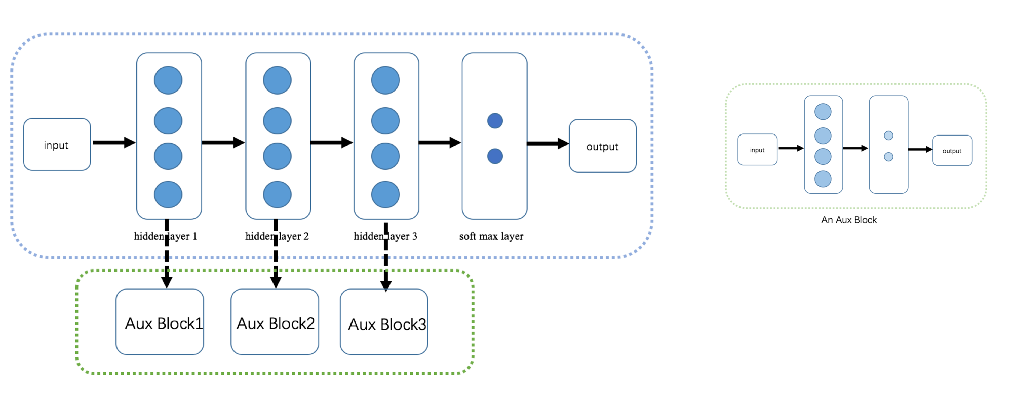
Figure 2: (Left) Blue dotted circular frame is the private of an original model, while green dotted frame is the private of Aux Blocks, an Aux Block can be any function.(right) An example of an Aux Block, an one hidden layer CNN.

Szegedy [20] first proposed to find adversarial examples in DNN models, he used L-BFGS algorithm to find them and observed that they catastrophically destroyed DNN models. They also observed that the transferability property of adversarial perturbations, one generated from an arbitrary model can also fool other models to produce incorrect outputs even if they are trained on different datasets with completely different structures. This phenomenon makes black-box attacks feasible.

Next, we discuss several attacking methods in our experiments.

Fast Gradient Sign Method: FGSM

Goodfellow er al. [7] proposed the FGSM method for crafting adversarial examples. FGSM is un-targeted and uses the same attack strength at every dimension:

$$x_{FGSM}=x+\epsilon\operatorname{sign}(\nabla_{x}J(x,y))$$

The above equation increases the loss function $J(\cdot)$ by adding a transformed gradient to input $x$, where $\epsilon$ is small enough to be undetectable.

There are several variants such as R+FGSM [21], BIM[12], and so on.

Projected Gradient Descent:PGD

Madry et al.[14] reviewed adversarial robustness in a max-min saddle point problem and suggested that BIM (Basic Iterative Method applies FGSM multiple times with small step size)[12] is a projected gradient descent method essentially. In the following sections, we will replace BIM by PGD. They conjectured that Projected Gradient Descent (PGD) is the strongest attack utilizing the local first order information about the network [14].

$$x_{N+1}=\Pi_{x+S}(x_{N}+\alpha(\nabla_{x}J(x,y)))$$

where $\alpha$ controls the magnitude of the perturbation in each iteration.

Carlini and Wagner’s Attacks

Carlini and Wagner proposed a high success rate method – optimization-based attack algorithms [6] to craft adversarial with low distortion. There are three versions based on different measures: $L_{2}$, $L_{0}$ and $L_{\infty}$. However, Carlini and Wagner’s attack is computationally expensive compared to FGSM. In our paper, we select Carlini and Wagner’s $L_{2}$ attack.

Boundary Attacks

Wieland et al.[3] introduced a decision-based attack which dose not rely on gradient of the model but the final decision boundary of the model. A random perturbation are crafted at first, reduced iteratively in the adversarial region. We will use this algorithm as a gradient-free attack.

II-C Defenses Methods

Adversarial Training is one of the most popular defense strategies, which is to train a model using both clean data and adversarial data [20, 7] to improve robustness. We study the adversarial training algorithm in [14] which solves a min-max problem:

$$\theta^{*}=\arg\min_{\theta}\mathop{\mathbb{E}}\limits_{x,y\in\mathcal{X}}\left[\max_{\sigma\in[-\epsilon,\epsilon]^{N}}J(x+\sigma,y)\right].$$

The authors solved the inner problem by crafting adversarial examples with projected gradient descent attacks.

Previous work has observed the phenomenon of gradient masking[1], which refers to a defense model with useless gradients by proposing a non-differentiable model [4] or representing data with less details [24]. Some defenses such as BRELU and MagNet are experimentally defeated with a small distortion[5]. Defensive Distillation[18] is also one of the most famous attack-agnostic techniques, which aims to make NN models more robust against all attacks but this method is not robust under Carlini and Wagner’s attack[6]. Moreover, most defenses obfuscate gradients somewhat, which indicate that the adversarial attack is still an unsolved problem and open for study.

II-D Threat Model

In our setting, we assume that an attacker have all knowledge of a model, such as the model parameters and model architectures in white-box attacks. Moreover, we introduce a clever attacker who is assumed to be aware of defenses that may be used.

As in Warren et al. [8], we consider two white-box attacks (ref. Table I):

Static Adversary

Attackers know everything about the model itself but do not realize any protection defense. A static Adversary is called partial white-box attacks in adversarial machine learning.

Adaptive Adversary

An adversarial examples are crafted and tailored for specific defenses by attackers. This is more difficult to resist compared with static adversary. In this paper, we consider both static and adaptive adversaries.

TABLE I: Threat model: adversary knows $\theta_{original}$ and/or $\theta_{defense}$

	$\theta_{original}$	$\theta_{defense}$
Black-box attack	unknown	unknown
Static attack	known	unknown
Adaptive attack	known	known

III Method

In this section, we illustrate our Aux Block model to improve neural network’s robustness. We will first introduce our algorithm and motivations, and then discuss some observations behind our algorithm.

Ensemble of several different models can improve robustness against malicious inputs. However, the straits of conventional ensemble methods are also apparent: storing and reloading $k$ different models is a huge burden on memory consumption, and tuning parameters in each model is a tricky task. In this paper, we propose an algorithm that is able to generate several auxiliary classifiers in one model with less memory cost and can avoid additional parameter tuning process.

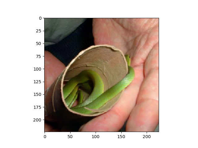
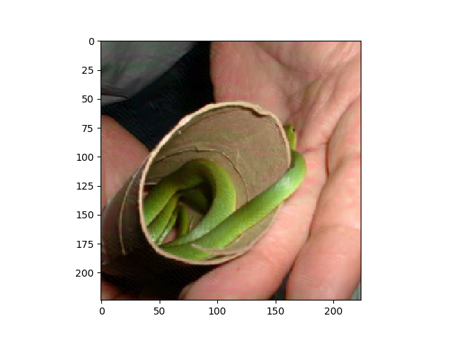
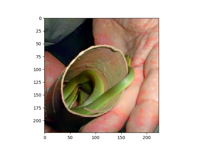
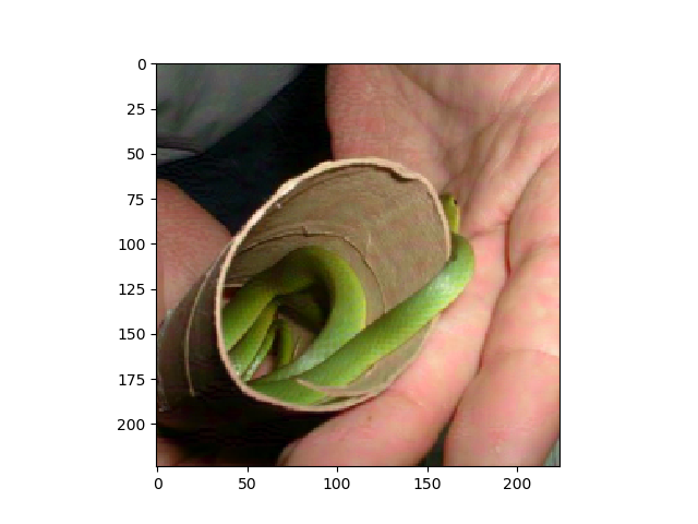
Figure 3: The first row shows the adp-inputs in the non-defense model, adversarial training model and our model on Mini-Imagenet dataset. The second row shows the perturbation images from Adp-PGD attacks in the three models.

III-A Model

Our main idea is to introduce Aux Block and then divide the model into two versions: a $public$ model and a $private$ model. More specifically, the $public$ model is a standard convolutional neural network and the $private$ is several branching auxiliary models as shown in Fig. 2. The $public$ model can be revealed to attackers while the $private$ model is confidential to them, so malicious hackers cannot create valid examples easily. An aux Block can be any structure, and in this paper we propose a tiny neural network.

Algorithm 1 Training and Testing of Aux Block

0:  $m$ Aux Blocks as $f_{A_{1}},f_{A_{2}},\cdots,f_{A_{m}}$ and an original CNN model as $f$.

  Training Phase:

  for $i=1,2,\cdots$ do

     Randomly sample $(x_{i},y_{i})$ in dataset

     Compute $loss=\sum\limits_{j=1}^{m}l(f_{A_{j}}(x_{i}),y_{i})+l(f(x_{i}),y_{i})$

     Compute $\Delta{w}=\nabla_{w}loss$

     Update $w\leftarrow w-\Delta{w}$

  end for

   Testing Phase:

  A testing image $x$

  for $j=1,2,\cdots,m+1$ do

     Calculate probability output of each Aux Block and the original model:

      $p_{j}=f_{A_{j}}(x)$, $\mathrm{if}\ j<m+1$ or $p_{j}=f(x)$, $\mathrm{if}\ j=m+1$

     Calculate each output $y^{j}=\arg\max_{k}p_{k}$

  end for

  Predict the class:

  for each label $k=1,2,\cdots,n$ do

     $Y_{k}=\sum\limits_{j=1}^{m+1}\ 1$,if $y^{j}=k$

  end for

  Predict the class $\hat{y}$,with $\hat{y}=\arg\max_{k}{Y_{k}}$.

Auxiliary network architectures are well-designed for several different datasets in the context of image classification. Details about the architectures will be discussed concretely in the next section. We denote an integral model as $f$, $x$ is the input image, and the output is an n-dimensional vector instead of a single value: $y=[y_{1},y_{2},y_{3},\dots,y_{m+1}],y\ \mathrm{in}\ \Re^{m}$ ($m$ is the number of Aux Blocks ), $y_{1}$ is the output of the $public$ network, while $y_{2},y_{3},\dots,y_{m+1}$ is from Aux Blocks. Since the malevolent examples are crafted without auxiliary information, predicted outputs are less likely to be misled in Aux Blocks. Therefore our model can be deployed in security-sensitive areas.

The new cross-entropy loss function is rewritten as:

$$Loss=-\sum\limits_{i=1}^{n}\alpha_{i}(\sum\limits_{j=1}^{T}y_{ij}\cdot\log P_{ij}),$$

where $T$ is the number of class labels, $y_{ij}$ denotes the value of label $j$ in classifier $i$ and $P_{ij}$ is classifying possibility for $y_{ij}$. Since the new loss function is an aggregation function from each classifier, $\alpha_{i}\in\Re$ is a parameter which controls the relative weight of $i$ classifier in the total loss, as the confidence of an Aux Block in the final decision. In this paper, we use $\alpha=1$ for all Aux Blocks.

Algorithm 2 A score-based Aux Block algorithm

  Similar steps as Algorithm 1

  Predict the class:

  We have the Aux Block weight $\alpha_{i}$ and the probability of class $k$ in Aux Block $j$ as $p_{jk}$.

  for $j=1,2,\cdots,m+1$  do

     Calculate softmax values from probability outputs in each Aux Block $s_{j}=[\frac{e^{p_{j0}}}{\sum\limits_{k=1}^{n}e^{{p}_{jk}}},\frac{e^{p_{j1}}}{\sum\limits_{k=1}^{n}e^{{p}_{jk}}},\cdots,\frac{e^{p_{jn}}}{\sum\limits_{k=1}^{n}e^{{p}_{jk}}}]$.

  end for

  Sum up the probability of all Aux Blocks and the original network $s=\sum\limits_{j=1}^{m+1}{\alpha_{i}s_{j}}$.

  Predict the class $\hat{y}$,with $\hat{y}=\arg\max{s}$.

Our algorithm is listed in Algorithm1. In the algorithm, we select the class $k$ which most Aux Blocks support as the final output. There are also other measures, such as a score-based algorithm with which the only difference is on selecting the final output. In Algorithm 2, we implement the same training phase but in the testing phase. We calculate values of each class and select the maximum value. Compared with Algorithm 1, Algorithm 2 evaluates probability of each class more discretely and considers that an Aux Block with larger $\alpha$ has a large weight in testing. We apply Algorithm 1 when $\alpha_{i}=1,\left(i=1,\cdots,m\right)$. Algorithm 1 becomes equivalent to Algorithm 2 .

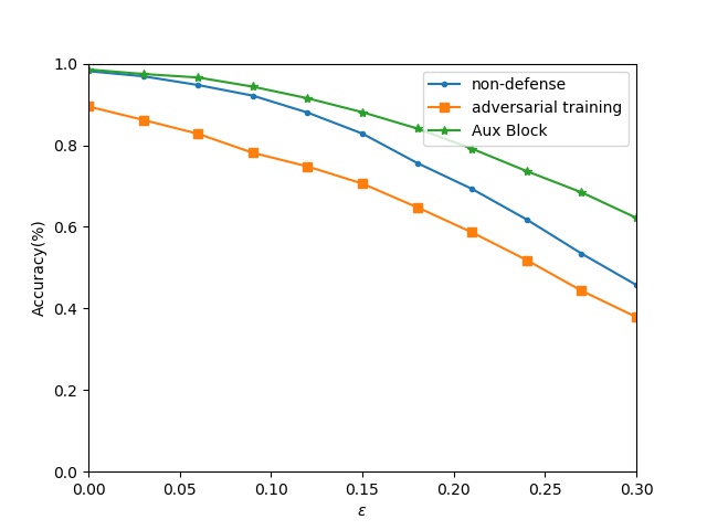
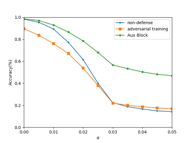
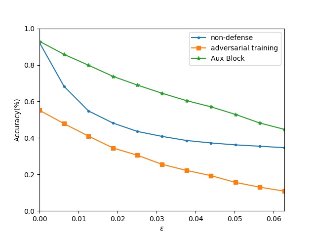
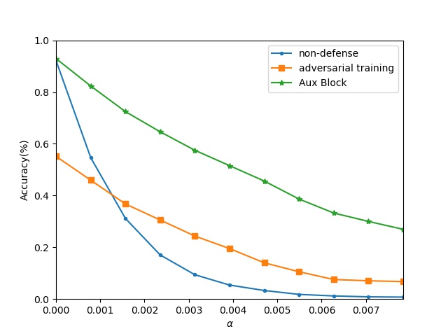
Figure 4: The first row shows the accuracy curves of Adp-FGSM and Adp-PGD on MNIST dataset. The second row shows the curves on CIFAR10 dataset.

III-B Discussion

In the static adversary, adversarial examples are crafted based on the non-defense model. So there can be two totally different approaches to defense these attacks. One is to reduce some necessary information, with which some existing defenses have used [23]. However, a defense performs well in a static adversary may be stock in the gradient masking phenomenon. Anish and Nicholas [1] observed that defending models based on gradient obfuscation is a false orientation.

Instead of information-reducing algorithms, our method increases the information by a combination output from all Aux Blocks and the original network. We do not obfuscate gradients in the original model, but an adversarial example crafted from the original model are blind to the extra knowledge in Aux Blocks.

In the adaptive adversary, masking gradient methods are like self-deceived. When an attacker realizes the defense, he or she can bypass the defense effortless then the defense has no any effect for adversarial examples. We propose a new attack Adp-FGSM to craft malicious examples from defense models straight. Our method can still improve robustness in this adversary. Though an attack crafts an adversarial image for our approach, the perturbation aims to mislead one Aux Block can be right classified by other Aux Blocks. We will give more explanations about this in Section 4.4.

IV Experiments

TABLE II: Comparisons of accuracies on MNIST, CIFAR10 and Mini-Imagenet datasets,

Dataset	Method	Clean	PGD	CW	Boundary Attack
MNIST	NA	98.88	21.26	0.0	0.2
	Adversarial Training	98.76	89.63	58.2	97.9
	Aux Block(all)	98.49	88.2	68.4	96.6
	Aux Block(private)	98.21	89.59	76.8	97.7
CIFAR10	NA	92.53	12.30	0.0	5.4
	Adversarial Training	83.89	78.82	76.7	83.5
	Aux Block(all)	91.72	74.44	77.1	87.1
	Aux Block(private)	89.74	77.72	77.5	90.0
Mini-Imagenet	NA	87.8	4.6	0.0	-
	Adversarial Training	72.9	68.5	75.2	-
	Aux Block(all)	86.7	67.9	84.9	-
	Aux Block(private)	85.2	71.6	86.0	-

IV-A Experiments setups

IV-A1 Datasets

Our experiments are performed on three datasets:

1. MNIST[13] contains 70,000 samples: 60,000 training samples and 10,000 testing samples. Each sample is a grayscale image with $28\times 28$ pixels. The number of possible classes is 10.

2. CIFAR10[10] contains 60,000 images in 10 classes: 50,000 training images and 10,000 testing images with $32\times 32$ pixels in RGB color channels.

3. We also test on Mini-Imagenet dataset with 10 classes randomly chosen from the 100 MiniImagenet classes [22] (each class with 600 images), on which a VGG16 model has been trained on 5000 images (500 images in each class) with 87.8 % top-1 accuracy.

We consider two convolutional neural networks: LeNet5 [13] and VGG16 [19]. The activation function in each network is RELU and loss function is cross-entropy function.

IV-A2 Defense

Adversarial training (AT) with adversarial examples crafted by PGD attacks [14]. On the MNIST dataset, we pre-train an AT model with the maximum perturbation $\epsilon=0.2$, step size $\alpha=0.02$, while on both CIFAR10 dataset and Mini-Imagenet dataset, $\epsilon$ is $8/255$ and $\alpha=2/255$.

IV-A3 Attacking Methods

In the static white-box adversary, we use the following attacks.

1. We implement PGD with 5 iterations: $\alpha=0.1,\epsilon=0.3$ on MNIST ,$\alpha=2/255,\epsilon=8/255$ on CIFAR10 and $\alpha=3/255,\epsilon=10/255$ on Mini-Imagenet.

2. We implement Carlini and Wagner’s $L_{2}$ attack as a targeted attack.

3. We implement Boundary attacks as a gradient-free attack.

While in the adaptive adversarial, we use the adaptive attacks. We modify FGSM and PGD to Adp-FGSM and Adp-PGD for the adaptive adversary, $x_{adv}$ are crafted from:

$$x_{adv}=x_{adp}+\epsilon(\nabla_{x_{adp}}J_{adp}(x_{adp},y)),$$

where $x_{adp}$ and $J_{adp}$ are re-designed on this particular defense.

Adversarial Training. We reassess that this algorithm transforms the original inputs to adversarial inputs, therefore we use the new input $x_{adp}=x+\Delta x$, where $\Delta x$ is the perturbation for Adversarial Training.

Aux Block. We use the loss function defined in Section 3 to fool all Aux Blocks and the original model together:

$$J_{adp}(x,y)=\sum\limits_{j=1}^{m}l(f_{A_{j}}(x),y)+l(f(x),y).$$

Fig.3 shows the adversarial examples from Adp-PGD.

TABLE III: Overview of Training Parameters: the MNIST converges after about 20 epochs; the CIFAR10 and Mini-Imagenet uses parameter decay and multi-step scheduler to ensure model convergence.

Parameter	MNIST	CIFAR10	Mini-Imagenet
Learning Rate	0.01	0.01	0.01
Momentum	0.5	0.9	0.9
Decay Delay	0	0.0005	0.0005
Batch Size	128	128	32
Epochs	20	100	100
Multi-step Scheduler	-	0.1 (50 epochs)	0.1 (50 epochs)

IV-A4 Implementation Details

The training hyper-parameters for all models selected are in Table III. We use a SGD optimizer during the training phase. Especially, we run pre-trained models for 5 epochs to get adversarial training models.

IV-B Aux Block Details

In this section, We review VGG16 structures as [64,64,M, 128,128,M, 256 ,256, 256, M, 512, 512, 512, M, 512,512, 512, M], one Aux Block model as Block.

The first question: Where is the suitable position of a Block?

The instinct is that features in high layers are easy to be contaminated and a small perturbation in one pixel is an accumulation of the large region, since features are more abstract and the receptive field of one pixel is large. In our experiment, we insert 3 Aux Blocks in three different position: [64,64,’Block1’, M, 128,128, M, 256,’Block2’,256, 256, M, 512, 512, 512, M, 512,’Block3’,512, 512, M]. We craft our Aux Block in Table IV.

Feature maps in each convolution layer are our inputs in an Aux Block. Since the feature size shrinks after filtering each maxpooling layer, we use a flexible Aux Block structure: the number of our Aux Block layer decreases if the size of a feature map diminishes.

TABLE IV: Aux Block

Layer	Parameters
Convolution + BatchNorm + ReLU	$7\times 7\times 96$, stride=2
MaxPool	$2\times 2$
Convolution + BatchNorm +ReLU	$3\times 3\times 192$
MaxPool	$2\times 2$
Convolution + BatchNorm +ReLU	$3\times 3\times 384$
MaxPool	$2\times 2$
Convolution + BatchNorm +ReLU	$3\times 3\times 512$
MaxPool	$2\times 2$
Fully Connected	$10$

As mentioned above, the three Aux Blocks have different structures: Block1 is same as Aux Block in TableIV, while Block2,Block3 is in TableV. Block3 only has a max pooling layer since the feature size is $2\times 2$.

TABLE V: The structure of Block2,Block3.

Layer	Parameters
MaxPool	$2\times 2$
Convolution + BatchNorm +ReLU	$3\times 3\times 384$
MaxPool	$2\times 2$
Convolution + BatchNorm +ReLU	$3\times 3\times 512$
MaxPool	$2\times 2$
Fully Connected	$10$
MaxPool	$2\times 2$
Fully Connected	$10$

TABLE VI: The accuracy of three different Block in different positions, Block1 has a highest rate.

private				public
	Block1	Block2	Block3	VGG16
PGD Attack	60.96	53.58	53.92	53.99

We use a two-iteration PGD to craft adversarial examples from the $public$ model and observe each Aux Block’s accuracy to investigate whether the position of an Aux Block will influence its robustness. The result in Table VI proposes that Block2 and Block3 have a same performance compared to the original result, while Block1 improves robustness to some extent. Therefore, we propose that deep layers are not a wise election for an Aux Block.

The second question: What is the number of Aux Blocks?

If we create a large number of Aux Blocks, it is inescapable to select feature maps in deep layers as inputs, which will not increase the robustness of our model but aggravate the weight of incorrect output for a score-based Aux Block model and make the model become too complicated. In our experiments, we choose the first three layers to add Aux Blocks.

The third question: What structure is suitable for an Aux Block?

A rough Aux Block will decrease the model accuracy of clean data, while the model will look overstaffed if an Aux Block is too meticulous. In this paper, we design three Aux Blocks as Aux1,Aux2,Aux3 for three datasets.

For MNIST, we use the model in Table:VIII and an Aux Bolck model in Table IX. For CIFAR10, the Aux Block structure is in Table X. For Mini-Imagenet, the structure is in Table XI.

IV-C Static Adversary Results

We show our method improves the test accuracy of adversarial examples in the static adversary. We randomly select 1000 samples for the boundary attack in the testing set and do not use this algorithm in Mini-Imagenet due to the shortage of computation.

In Table II, our model outputs two values: one is the result from the whole system and the other is only from Aux Blocks as private results. Compared to adversarial training, Aux Block(private) has a better or equivalent performance, which illustrates that adversarial examples from the original non-defense model can be resisted by the Aux Block model. Particularly, our method’s performance is better than adversarial training against Carlini and Wagner’s attack on all datasets。

IV-D Adaptive Adversary Results

Compared with the static adversary, an adaptive adversary is a more challenging circumstance to defense. The attacker bypasses the original no-defense model and crafts specific examples from defense models straightforward.

IV-D1 Results

Table VII shows the accuracy on the Adp-PGD attacks. In this table, our model outperforms the adversarial training model remarkably 56.55% and 54.6% on Mnist and Cifar10 dataset, while adversarial training models only have about 20% accuracy.

TABLE VII: The accuracy in an adaptive adversary, with Adp-PGD attacks

	MNIST	CIFAR10	Mini-Imagenet
NA	21.30	6.95	6.24
Adversarial Training	22.10	22.05	25.5
Aux Block	56.55	54.6	38.7

Fig. 4 also shows Aux Block model helps to improve the accuracy of adversarial examples. For small perturbation, even if the attacker know how to craft adversarial examples for our Aux Block model, it is still able to improve robustness compared to adversarial training models. However, as observed in the experiments, if the perturbation is large enough, our Aux Block model will also be collapsed.

Although the experiment concerns with un-targeted attacks, it does not mean targeted attacks are not covered. As we know, targeted attacks are harder to attack and easier to defense.

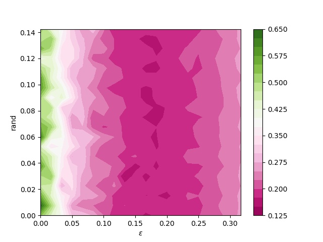
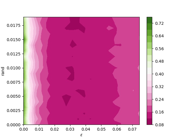
Figure 5: Left: In the MNIST dataset, the ratio of the average value $l_{avg}$ to the loss value $l_{i}$ from the Adp-FGSM perturbation with a random initial. A small ratio value represents the average loss value is less than the targeted loss. Right: A figure in the CIFAR10 dataset.

IV-D2 Interpretation

An adversarial example should fool most of Aux Blocks to mislead our method. We assume an attack for one Block is not sufficient to fool other Blocks and crafting an example to fool all Blocks together is more difficult than fooling one. Therefore, our model is less likely to be collapsed than non-defense one.

To prove an attack for one Block is not sufficient to fool other Blocks, we investigate the loss value in our Aux Block model. We craft the specific perturbation targeted to one Aux Block, and then observe the loss value of this adversarial example in the selected classifier and also the average value in others. For example, the adversarial example $x_{adv}=x+\sigma_{i}$, where $\sigma_{i}$ is the perturbation for Aux Block $i$. Therefore, the first loss value is $l_{i}=l\left(f_{i}(x_{adv}),y\right)$ and the second value is $l_{avg}=\frac{1}{m}\sum_{k=1,k\neq i}^{m+1}l\left(f_{k}\left(x_{adv}\right),y\right)$.

Other auxiliary classifiers are not sensitive to the perturbation from the targeted classifier in Fig. 5, since the ratio is less than 1 especially when the perturbation is not very large. One severe attack for an Aux Block has only slight influence to other Aux Blocks. We can see that random value do not effect the ratio. Moreover, it is obvious that crafting an example to fool all Blocks together is more difficult than fooling one. Therefore our method is still robust in the presence of adaptive white-box adversaries.

V Conclusion and outlook

TABLE VIII: MNIST Model

Layer	Parameters
Convolution + ReLU	$5\times 5\times 6$
MaxPool	$2\times 2$
Convolution + ReLU	$5\times 5\times 16$
MaxPool	$2\times 2$
Fully Connected	$120$
Fully Connected	$10$

TABLE IX: Aux Block in MNIST Model

Layer	Parameters
Fully Connected	$200$
Fully Connected	$10$

In this paper, we propose a new defense technique called the Aux Block model to improve the robustness of neural networks against adversarial perturbations. We show that our algorithm is a self-ensemble model and the experimental results demonstrates that our model is robust in both two adversaries and reports significantly improved empirical results in real applications. Hence, our work lays out a new framework for adversarial machine learning.

We suggest two lines of work for future study of the model. On one hand, more applications are expected other than the image classification applications that has been investigated in this paper. On the other hand, a theoretical analysis of the method is necessary to better understand the application scopes of the proposed model.

TABLE X: Aux Block in Cifar10

Layer	Parameters
Convolution + BatchNorm + ReLU	$9\times 9\times 64$ (stride=4)
Convolution + BatchNorm +ReLU	$3\times 3\times 256$
MaxPool	$2\times 2$
Convolution + BatchNorm +ReLU	$3\times 3\times 256$
MaxPool	$2\times 2$
Fully Connected	$200$
Fully Connected	$10$

TABLE XI: Aux Block in Mini-Imagenet

Layer	Parameters
Convolution + BatchNorm + ReLU	$9\times 9\times 64$ (stride=4)
Convolution + BatchNorm +ReLU	$3\times 3\times 256$ (stride=2)
MaxPool	$2\times 2$
Convolution + BatchNorm +ReLU	$3\times 3\times 256$
MaxPool	$2\times 2$
Convolution + BatchNorm +ReLU	$3\times 3\times 512$
MaxPool	$2\times 2$
Fully Connected	$512$
Fully Connected	$10$

References

- [1] A. Athalye, N. Carlini, and D. Wagner. Obfuscated gradients give a false sense of security: Circumventing defenses to adversarial examples. arXiv preprint arXiv:1802.00420, 2018.
- [2] B. Biggio, I. Corona, D. Maiorca, B. Nelson, N. Šrndić, P. Laskov, G. Giacinto, and F. Roli. Evasion attacks against machine learning at test time. In Joint European conference on machine learning and knowledge discovery in databases, pages 387–402. Springer, 2013.
- [3] W. Brendel, J. Rauber, and M. Bethge. Decision-based adversarial attacks: Reliable attacks against black-box machine learning models. arXiv preprint arXiv:1712.04248, 2017.
- [4] J. Buckman, A. Roy, C. Raffel, and I. Goodfellow. Thermometer encoding: One hot way to resist adversarial examples, 2018.
- [5] N. Carlini and D. Wagner. Magnet and “efficient defenses against adversarial attacks” are not robust to adversarial examples. arXiv preprint arXiv:1711.08478, 2017.
- [6] N. Carlini and D. Wagner. Towards evaluating the robustness of neural networks. In 2017 IEEE Symposium on Security and Privacy (SP), pages 39–57. IEEE, 2017.
- [7] I. Goodfellow, J. Shlens, and C. Szegedy. Explaining and harnessing adversarial examples. In International Conference on Learning Representations, 2015.
- [8] W. He, J. Wei, X. Chen, N. Carlini, and D. Song. Adversarial example defenses: Ensembles of weak defenses are not strong. arXiv preprint arXiv:1706.04701, 2017.
- [9] G. Hinton, L. Deng, D. Yu, G. E. Dahl, A.-r. Mohamed, N. Jaitly, A. Senior, V. Vanhoucke, P. Nguyen, T. N. Sainath, et al. Deep neural networks for acoustic modeling in speech recognition: The shared views of four research groups. IEEE Signal processing magazine, 29(6):82–97, 2012.
- [10] A. Krizhevsky and G. Hinton. Learning multiple layers of features from tiny images. Technical report, Citeseer, 2009.
- [11] A. Krizhevsky, I. Sutskever, and G. E. Hinton. Imagenet classification with deep convolutional neural networks. In Advances in neural information processing systems, pages 1097–1105, 2012.
- [12] A. Kurakin, I. Goodfellow, and S. Bengio. Adversarial examples in the physical world. arXiv preprint arXiv:1607.02533, 2016.
- [13] Y. LeCun, L. Bottou, Y. Bengio, and P. Haffner. Gradient-based learning applied to document recognition. Proceedings of the IEEE, 86(11):2278–2324, 1998.
- [14] A. Madry, A. Makelov, L. Schmidt, D. Tsipras, and A. Vladu. Towards deep learning models resistant to adversarial attacks. arXiv preprint arXiv:1706.06083, 2017.
- [15] S.-M. Moosavi-Dezfooli, A. Fawzi, and P. Frossard. Deepfool: a simple and accurate method to fool deep neural networks. In Proceedings of the IEEE Conference on Computer Vision and Pattern Recognition, pages 2574–2582, 2016.
- [16] V. Nair and G. E. Hinton. Rectified linear units improve restricted boltzmann machines. In Proceedings of the 27th international conference on machine learning (ICML-10), pages 807–814, 2010.
- [17] N. Papernot, P. McDaniel, S. Jha, M. Fredrikson, Z. B. Celik, and A. Swami. The limitations of deep learning in adversarial settings. In Security and Privacy (EuroS&P), 2016 IEEE European Symposium on, pages 372–387. IEEE, 2016.
- [18] N. Papernot, P. McDaniel, X. Wu, S. Jha, and A. Swami. Distillation as a defense to adversarial perturbations against deep neural networks. In 2016 IEEE Symposium on Security and Privacy (SP), pages 582–597. IEEE, 2016.
- [19] K. Simonyan and A. Zisserman. Very deep convolutional networks for large-scale image recognition. arXiv preprint arXiv:1409.1556, 2014.
- [20] C. Szegedy, W. Zaremba, I. Sutskever, J. Bruna, D. Erhan, I. Goodfellow, and R. Fergus. Intriguing properties of neural networks. arXiv preprint arXiv:1312.6199, 2013.
- [21] F. Tramèr, A. Kurakin, N. Papernot, I. Goodfellow, D. Boneh, and P. McDaniel. Ensemble adversarial training: Attacks and defenses. arXiv preprint arXiv:1705.07204, 2017.
- [22] O. Vinyals, C. Blundell, T. Lillicrap, D. Wierstra, et al. Matching networks for one shot learning. In Advances in neural information processing systems, pages 3630–3638, 2016.
- [23] W. Xu, D. Evans, and Y. Qi. Feature squeezing: Detecting adversarial examples in deep neural networks. arXiv preprint arXiv:1704.01155, 2017.
- [24] V. Zantedeschi, M.-I. Nicolae, and A. Rawat. Efficient defenses against adversarial attacks. In Proceedings of the 10th ACM Workshop on Artificial Intelligence and Security, pages 39–49. ACM, 2017.