Abstract

In this work, we present an algorithm for the design of $n\times n$-bits substitution boxes (S-boxes) based on time series of a discrete dynamical system with chaotic behavior. The elements of a $n\times n$-bits substitution box are given by binary sequences generated by time series with uniform distribution. Particularly, time series with uniform distribution are generated via two lag time chaotic series of the logistic map. The aim of using these two lag time sequences is to hide the map used, and thus U-shape distribution of the logistic map is avoided and uncorrelated S-box elements are obtained. The algorithm proposed is simple and guarantees the generation of S-boxes, which are the main component in block cipher, fulfill the strong S-box criteria: bijective; nonlinearity; strict avalanche criterion; output bits independence criterion; criterion of equiprobable input/output XOR distribution and; maximum expected linear probability. The S-boxes that fulfill these criteria are commonly known as “good S-boxes”. Finally, an application based on polyalphabetic ciphers principle is developed to obtain uniform distribution of the plaintext via dynamical S-boxes.

S-box; block cipher; dynamical S-Box; chaos; lag time chaotic series.

1 Introduction

Nowadays, we are in the era of informatics and due to the large number of attacks, it is important to adequately protect the information to avoid possible misuse of it. The aforementioned comment motivates the generation of different approaches to have secure cryptographic systems. In general cryptosystems can be divided in two classes: stream cipher and block cipher. The stream cipher combines bit to bit, the sequences of bits generated by plaintext and pseudorandom numbers. The block cipher takes blocks of plaintext which are encrypted by substitution using an S-box and cyclic shifting. The substitution box (S-box) is the core component of block cipher. The S-boxes give the cryptosystems the confusion property described by Shannon [1], used in conventional block ciphers such as the Data Encryption Standard (DES) and the Advanced Encryption Standard (AES). In these cryptosystems the security depends mainly on the S-box properties that are used. The criteria that a strong S-box fulfill, also known as “good S-boxes”, are: bijection; nonlinearity; strict avalanche criterion (SAC); the output bit independence criterion (BIC) [2]. Other desirable characteristics are to be resistant to linear and differential cryptanalysis attacks. The construction of cryptographically secure S-boxes is a field of interest in the cryptography area.

In recent years, many papers have been reported and are focused on studying cryptosystems based on chaos [3, 4, 5, 6, 7, 8, 9, 10, 11, 12], this is, because of the relationship that exists between the chaotic system properties and the cryptosystem properties. In [13] the relationship between these properties are given, for instance, confusion is related with ergodicity, the diffusion property with sensitivity to initial conditions and the deterministic dynamic with the deterministic pseudo-randomness. Taking advantage of the properties of chaotic systems, we propose a strong and dynamic S-Box that complies with the different criteria of good S-boxes.

Regarding the generation of S-box based on chaos, some algorithms have been developed using discrete dynamical systems. For example, in [3, 4, 5, 6, 7], the generation of substitution boxes were introduced through a single time series of a map or by combining two time series of different maps. Nevertheless, these algorithms do not guarantee that the series used have a uniform distribution, as in our approach based on two lag time chaotic series derived from the logistic map. In the same way, there are algorithms based on continuous chaotic dynamical systems [8, 9, 10]. Also there are algorithms based on the mixing of time series of continuous and discrete dynamical systems [11, 12] and in [14] the algorithm is build via time-delay series. The advantage of using discrete chaotic dynamical systems is that from one iteration to another the elements of the time series are de-correlated, however this does not happen if a continuous chaotic dynamical system is used, the elements of the time series are strong correlated. Therefore, many iterations are needed and the calculation of the mutual information between elements of the time series is necessary to be able to say when they are de-correlated, which implies higher computational cost.

In chaos-based encryption schemes, pseudo-random sequences based on chaotic maps are generally used as one time pad for encrypting messages. Since encryption schemes, based on low dimensional chaotic map, have low computational complexity, they can be analyzed with low computational cost using iteration and correlation functions [15]. Time-delay chaotic series have complex behavior and erase the trace of the mapping that generates them. Using these aforementioned time series, S-boxes can be designed and provide better nonlinearity criterion, that ensure good statistical properties in the generators.

In this paper, a method to obtain dynamical good S-boxes is presented based on the generation of lag time series from the logistic map. Using this kind of lag time series, it is possible to generate S-boxes that have the capability of hiding the map used to build them. With this approach, based on these lag time series, pseudo-random series are generated with good statistical properties, more details can be found in [16]. This novel algorithm for S-box generation is based on cryptographically secure pseudo-random number generator. The rest of the paper is organized as follows: In Section 2, the criteria for a “good” $n\times n$ bit S-box are described. In Section 3, it is presented a dynamical analysis of logistics map. In Section 4, the proposed scheme to generate dynamical S-box based on pseudo-random bit generator is presented. In Section 5, the performance analysis of an obtained S-box and its comparison with other S-box reported in the literature is given. An application of the obtained S-boxes to hide an image is presented in Section 6. Finally conclusions are drawn in Section 7.

2 Criteria for a good n$\times$n bit S-box

A collection of six criteria reported in the literature for generate cryptographically good S-boxes has been made. These criteria are: bijective; nonlinearity; strict avalanche criterion; output bits independence criterion, equiprobable input/output XOR distribution; and maximum expected linear probability. Before addressing these properties it is necessary to give some preliminaries about Boolean functions.

Let $\mathbb{B}=\{0,1\}$ be a binary set which is endowed with two binary operations, called addition (denoted by $\oplus$ XOR operation) and multiplication (denoted by $\cdot$ AND operation). Let $(\mathbb{B},\oplus,\cdot)$ be a field which will be denoted by $\mathbb{F}$, where the binary operations are given by the table 1.

$\oplus$	0	1
0	0	1
1	1	0

$\cdot$	0	1
0	0	0
1	0	1

Table 1: Addition and multiplication binary operations.

An $n\times n$ S-box is a vectorial Boolean function $S:\mathbb{F}^{n}\to\mathbb{F}^{n}$, where $\mathbb{F}^{n}$ is a vectorial space, and is defined as:

(1) $$S(x)=(f_{1}(x),f_{2}(x),\cdots,f_{n}(x)),$$

where $x=(x_{1},x_{2},\cdots,x_{n})^{\top}\in\mathbb{F}^{n}$ and each of $f_{i}^{\prime}$s for $1\leq i\leq n$ is a Boolean function. A Boolean function is a mapping $f:\mathbb{F}^{n}\to\mathbb{F}$ by considering all inputs in $f$, $f_{i}$ can be seen as a column vector of $2^{n}$ elements. The functions $f_{i}^{\prime}$s are component functions of $S$.

Some basic definitions can be found in [17].

Definition 2.1.

A Boolean function with algebraic expression, where the degree is at most one is called an affine Boolean function. The general form for n-variable affine function is:

$$f_{affine}(x_{1},x_{2},x_{3},\ldots,x_{n})=w_{n}\cdot x_{n}\oplus w_{n-1}\cdot x_{n-1}\oplus\ldots\oplus w_{2}\cdot x_{2}\oplus w_{1}\cdot x_{1}\oplus w_{0},$$

where $w_{i}\in\mathbb{B}$ are coefficients, and $x_{i}\in\mathbb{B}$ are variables, with $i=0,1,\ldots,n$.

Definition 2.2.

A linear Boolean function is defined as follows

$$L_{w}(x)=w_{n}\cdot x_{n}\oplus w_{n-1}\cdot x_{n-1}\oplus\ldots\oplus w_{1}\cdot x_{1},$$

where $x_{i},w_{i}\in\mathbb{B}$, with $i=1,\ldots,n$.

The set of affine Boolean functions is comprised by the set of linear Boolean functions and their complements,i.e., all functions of the form

$$A_{w,c}(x)=L_{w}(x)\oplus c,\;c\in\mathbb{B}.$$

A useful representation of a Boolean function $f_{i}$, with $i=1,\ldots,n$, is given by the polarity truth table defined as follows.

Definition 2.3.

A polarity truth table is defined as follows

$$\hat{f}(x)=(-1)^{f(x)},$$

where $x\in\mathbb{F}^{n}$, $\hat{f}$ maps the output values of the Boolean function from the set $\{0,1\}$ to the set $\{-1,1\}$, $i.e.$,

$$\hat{f}:\{0,1\}\to\{-1,1\}.$$

A linear Boolean function in polarity form is denoted as $\hat{L}_{w}(x)$.

Definition 2.4.

The Walsh Hadamard transform (WHT) of a Boolean function $f$ is defined as

$$\hat{F}_{f}(w)=\sum_{x\in\mathbb{B}^{n}}{\hat{f}(x)\hat{L}_{w}(x)}.$$

The WHT measures the correlation between the Boolean function $f$ and the linear Boolean function $\hat{L}_{w}$ with $x\in\mathbb{F}^{n}$.

2.1 Bijective Criterion

Let $S(x)$ be an S-box, which is bijective if and only if their Boolean functions $f_{i}$ satisfy the following condition:

(2) $$wt(a_{1}\cdot f_{1}\oplus a_{2}\cdot f_{2}\oplus\cdots\oplus a_{n}\cdot f_{n})=2^{n-1},$$

where $a_{i}\in\mathbb{F}$, $(a_{1},a_{2},\cdots,a_{n})\neq(0,0,\cdots,0)$ and $wt(\cdot)$ is the Hamming weight [2, 18], the corresponding S-box is guaranteed to be bijective.

2.2 Nonlinearity criterion

Definition 2.5.

[19] The nonlinearity of a Boolean function $f:\mathbb{F}^{n}\to\mathbb{F}$ is denoted by

(3) $$N_{f}=\min_{l\in A_{w,c}(x)}d_{H}(f,l),$$

where $A_{w,c}(x)$ is an affine function set, $d_{H}(f,l)$ is the Hamming distance between $f$ and $l$.

The minimum distance between two Boolean functions can be described by means of the Walsh spectrum [20]:

(4) $$\min_{l\in A_{w,c}(x)}d_{H}(f,l)=2^{n-1}(1-2^{-n}\max_{\omega\in\mathbb{F}^{n}}|\hat{S}_{(f)}(\omega)|),$$

where the Walsh spectrum of $f(x)$ is defined as follows:

(5) $$\hat{S}_{(f)}(\omega)=|\hat{F}_{f}(w)|_{w\in\mathbb{B}^{n}}=\sum_{x\in\mathbb{F}^{n}}(-1)^{f(x)\oplus x\bullet\omega},$$

with $\omega\in\mathbb{F}^{n}$ and $x\bullet\omega$ is the dot product between $x$ and $\omega$ as:

(6) $$x\bullet\omega=x_{1}\cdot\omega_{1}\oplus\cdots\oplus x_{n}\cdot\omega_{n}.$$

2.3 Strict Avalanche Criterion (SAC)

This criterion was first introduced by Webster and Tavares [21]. A Boolean function $f$ satisfies SAC if complementing any single input bit changes the output bit with the probability one half. So, more formally, a Boolean function $f$ satisfies SAC, if and only if

(7) $$\sum_{x\in\mathbb{F}^{n}}f(x)\oplus f(x\oplus e_{i})=2^{n-1},~{}~{}~{}\forall i:1\leq i\leq n,$$

where $e_{i}\in\mathbb{F}^{n}$ such that $wt(e_{i})=1$.

2.4 Output Bits Independence Criterion (BIC)

Output Bit Independence Criterion is another desirable criterion for an S-box that should be satisfied, introduced by Webster and Tavares [21]. It means that all the avalanche variables should be pairwise independent for a given set of avalanche vectors generated by the complementing of a single plaintext bit.

Adam and Tavares introduced another method to measure the BIC that for the Boolean functions, $f_{i}$ and $f_{j}$ $(i\neq j)$ of two output bits in a S-box, if $f_{i}\oplus f_{j}$ is highly nonlinear and come as close as possible to satisfy SAC [2]. Additionally, $f_{i}\oplus f_{j}$ can be tested with a Dynamic Distance (DD). The DD of a function $f$ can be defined as:

(8) $$DD(f)=\max_{\begin{subarray}{c}d\in\mathbb{F}^{n}\\ wt(d)=1\end{subarray}}\frac{1}{2}\left|2^{n-1}-\sum_{x=0}^{2^{n}-1}f(x)\oplus f(x\oplus d)\right|.$$

If the value of DD is a small integer and close to zero, the function $f$ satisfies the SAC.

2.5 Criterion of equiprobable Input/Output XOR Distribution

Biham and Shamir [22] introduced differential cryptanalysis which attacks S-boxes faster than brute-force attack. It is desirable for an S-box to have differential uniformity. This can be measured by the maximum expected differential probability (MEDP). Differential probability for a given map $S$ can be calculated by measuring differential resistance and is defined as follows:

(9) $$DP_{f}=\max_{\Delta x\neq 0,\Delta y}\left(\frac{\#\{x\in\mathbb{F}^{n}|S(x)\oplus S(x\oplus\Delta x)=\Delta y\}}{2^{m}}\right),$$

where $2^{n}$ is the cardinality of all the possible input values ($x$), $\Delta x$ and $\Delta y$ are called input and output differences, respectively, for the $S$. Thus, the smaller value of $DP_{f}$ gives better cryptographic property, i.e., its resistance to differential cryptanalysis.

2.6 Maximum Expected Linear Probability

The Maximum Expected Linear Probability (MELP) is the maximum value of the unbalance of an event. Given two randomly selected masks $a$ and $b$, and $a$ is used to calculate the mask of all possible values of an input $x$, and use $b$ to calculate the mask of the output values of the corresponding S-box. The parity of the input bits mask $a$ is equal to the parity of the output bits the mask $b$. MELP of a given S-box can be computed by the following equation:

(10) $$LP_{f}=\max_{a,b\in\mathbb{F}^{n}\backslash\{0\}}\left(2^{-n}\sum_{x\in\mathbb{F}^{n}}(-1)^{a\cdot x+b\cdot f(x)}\right)^{2}.$$

The closer is MELP to zero, the higher the resistance against linear cryptanalysis attack will be.

3 Analysis of the Logistic map

The logistic map is a discrete-time demographic model analogous to the logistic equation first created by Pierre François Verhulst, which is described by the following differential equation

$$\frac{dx}{dt}=rx\left(1-\frac{x}{K}\right),$$

where $x$ is the state variable of the system, $r$ is a parameter related with the rate of maximum population growth and $K$ is the so-called carrying capacity (i.e., the maximum sustainable population). So $x\leq K$, when $x=K$ the population stops growing. Robert May [23] popularized this differential equation to one of the most famous discrete dynamical systems, the logistic map, which is defined as follows:

(11) $$f_{\alpha}(x_{i})=\alpha x_{i}(1-x_{i}),$$

where $x$ is the state variable of the logistic map and, $\alpha$ is the only parameter of the system instead of two as its analogous continuous model. The use of a single parameter was possible because the logistic map was normalized, i.e., $f_{\alpha}:[0,1]\to[0,1]$, for the bifurcation parameter $\alpha\in[0,4]$ and $x_{0}\in[0,1]$. Nevertheless, in the context of mathematics, the values of the parameter $\alpha$ are not restricted to the interval $[0,4]$, so mathematically, it is possible to consider negative values [24]. As mentioned above, the logistic map is now studied in the interval $[-2,0)$ for cryptographic purposes. Now, we study the mapping behavior in the two intervals and they assured with $\alpha\in[-2,4]$ the orbits do not scape to infinity for some initial conditions.

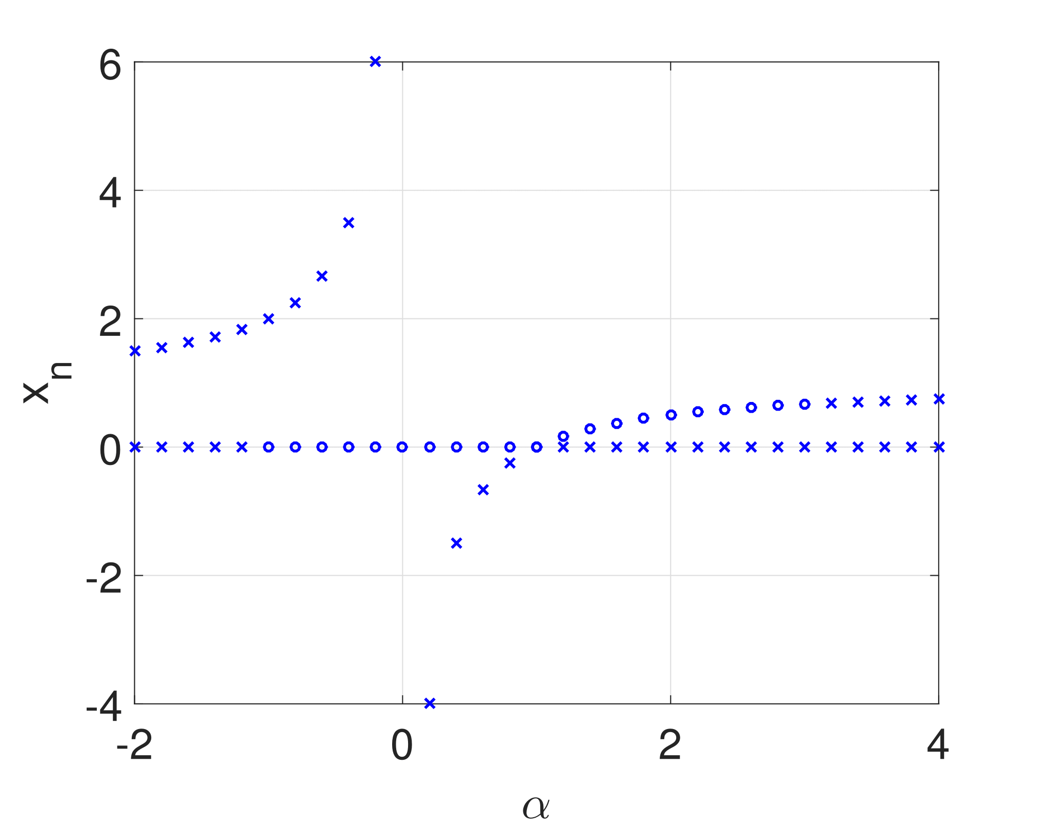
Figure 1: Fixed points stability where an asterisk and a circle denote repulsive and attracting fixed points, respectively.

The dynamical system (11) presents one or two fixed points located at $x^{*}_{1}=0$ and at $x^{*}_{2}=\frac{\alpha-1}{\alpha}$, for $\alpha\neq 0$. Figure 1  depicts the stability of the fixed points where an asterisk and a circle denote repulsive and attracting fixed points, respectively. These fixed points change their stability according to the parameter $\alpha$, i.e., when $|f^{\prime}(x^{*}_{1})|<1$ and $|f^{\prime}(x^{*}_{2})|<1$ then the fixed points $x^{*}_{1}$ and $x^{*}_{2}$ are stable, respectively, and they are unstable when $|f^{\prime}(x^{*}_{1})|>1$ and $|f^{\prime}(x^{*}_{2})|>1$. We are interested in the last case because the system presents complex behavior, this is, both fixed points are repulsive, $|f^{\prime}(x^{*}_{1})|=|\alpha|>1$ and $|f^{\prime}(x^{*}_{2})|=|-\alpha+2|>1$. The $x^{*}_{1}$ fixed point is repulsive for $\alpha<-1$ and $\alpha>1$. On the other hand, the $x^{*}_{2}$ fixed point is repulsive for $\alpha<1$ but $\alpha\neq 0$, and $\alpha>3$. So the interested values are $\alpha\in[-2,-1]\cup[3,4]$, this is the condition to have both repulsive fixed points.

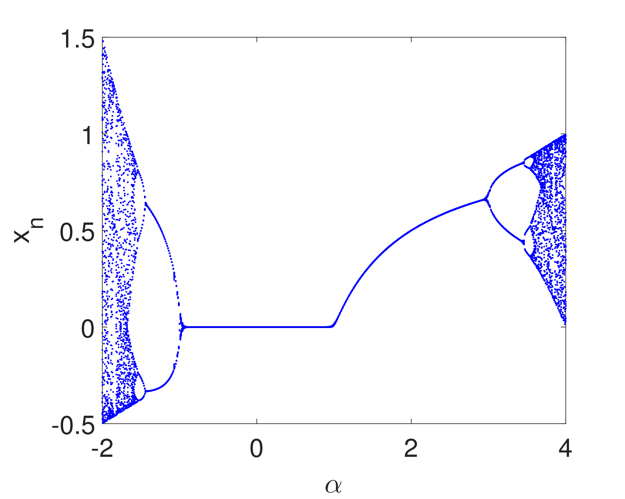
Figure 2: Bifurcation diagram for the logistic map given by Eq. (11).

The dynamical system (11) bifurcates when $|f^{\prime}(x^{*}_{1})|=1$ and $|f^{\prime}(x^{*}_{2})|=1$, this happens for $x^{*}_{1}$ when $\alpha=-1$ or $1$, and for $x^{*}_{2}$ the bifurcations values are given by $\alpha=1$ and $3$. It is possible to analyze the behavior of the system by means of a bifurcation diagram, which is shown in Figure 2. This diagram shows orbits as a function of $\alpha$ parameter and the route to chaos are period-doubling bifurcations at $\alpha=3$ and period-halving bifurcations at $\alpha=-1$. There are intervals for the parameter $\alpha$ near to $-2$ and $4$ where the logistic map $f_{\alpha}(x)$ behaves chaotically.

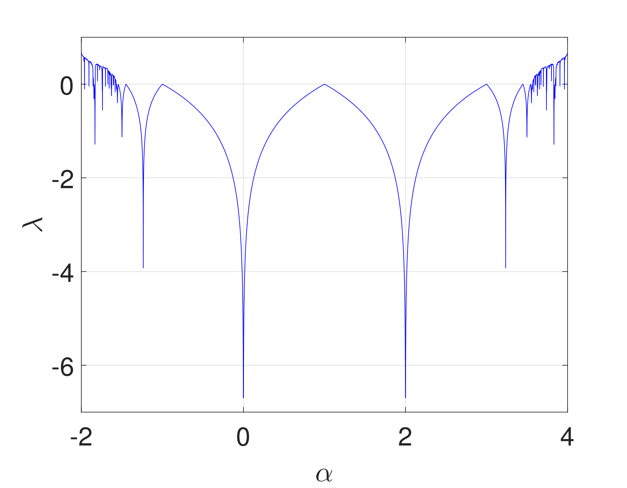
Figure 3: Lyapunov exponent as a function of parameter $\alpha$.

There are several approaches to demonstrate that a system is chaotic, one of them is prove that the dynamical systems fulfills the definition given by Devaney [25], other approach is based on the Lyapunov exponent [26],[27]. In the same sense, the Lyapunov exponent of Eq. 11 it is shown in Fig. 3. The graph of Lyapunov exponents is symmetric with respect to $\alpha=1$, the chaotic behavior of the logistic map appears for values of the parameter $\alpha$ near $-2$ and $4$. The local stability of the fixed points are in accordance with the Lyapunov exponent values, for example, when $\alpha\in(-1,3)$ the orbits of the system converge at a fixed point and, when the bifurcations occurs the orbits converge at periodic orbits up to chaos appears.

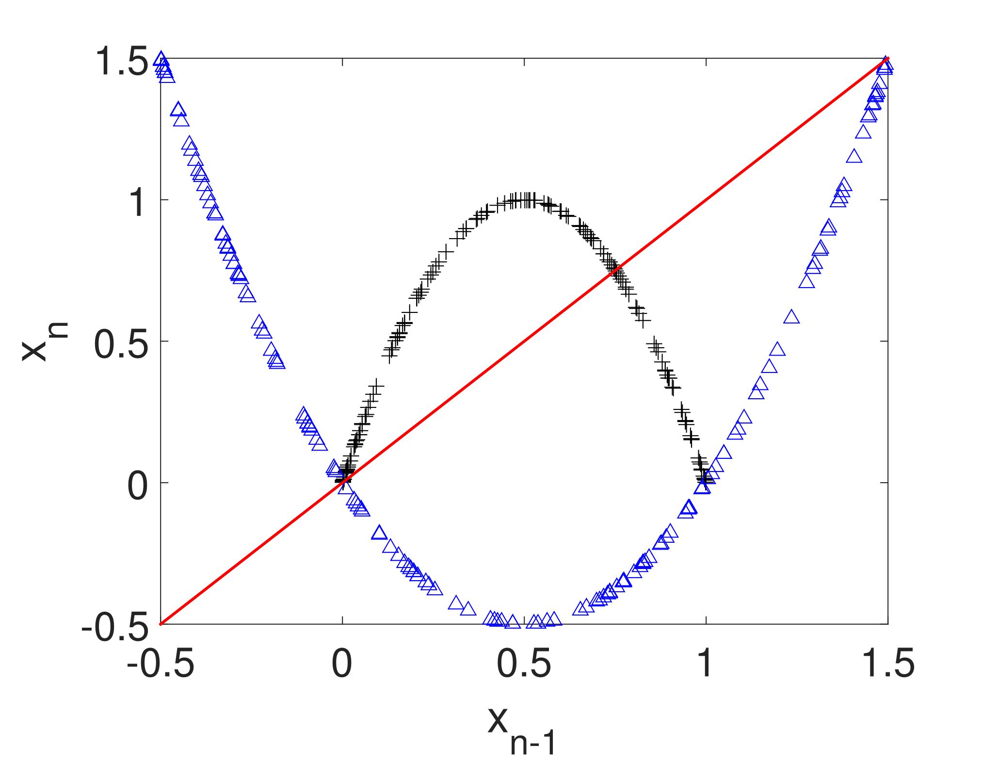
Figure 4: Logistic map for $\alpha=-2$ in blue triangles and for $\alpha=4$ in black crosses.

The aim is to use the logistic map to generate a time series with uniform distribution and without evidencing the mapping used. To achieve this, it is proposed an approach based on two chaotic time series of the logistic map. Based on Lyapunov exponents analysis, the $\alpha$ values are arbitrarily selected within the chaos region, so it is consider $\alpha=-2$ and $4$. In Figure 4 is presented the shape of the logistic map for both parameter values $\alpha=-2$ and $\alpha=4$ in blue triangles and in black crosses, respectively. The logistic map for these parameter values is invariant in different intervals as follows

(12) $$\begin{array}[]{rl}f_{-2}&:[-0.5,1.5]\to[-0.5,1.5];\\ f_{4}&:[0,1]\to[0,1].\end{array}$$

It is worth saying that the time series generated with both parameter values have a U-shape distribution.

4 Proposed algorithm to generate dynamical S-boxes

The main idea of the proposed algorithm to generate dynamical S-boxes is based on a Cryptographically Secure Pseudo-Random Number Generator (CSPRNG) via a discrete dynamical system $f_{\alpha}:I\to I$. García Martínez and Campos Cantón [16] proposed a CSPRNG using two lag time series generated with the logistic map (11).

An orbit $x_{0},x_{1},x_{2},\ldots$ of the logistic map (11) is defined by giving an initial condition $x_{0}\in I$. The interval $I$ is determined by the parameter $\alpha\in\{-2,4\}$, $f_{\alpha}:I\to I$. Let $M1$ and $M2$ two time series generated with the logistic map by means of the following considerations: i) given two arbitrary initial conditions $x_{01}$, $x_{02}$, such that, $x_{01}\neq x_{02}$; ii) two different bifurcation parameters $\alpha_{1}$ and $\alpha_{2}$; and iii) $l$-units of memory for each time series $x_{(i-k_{l-1})1}$, $\ldots$, $x_{(i-k_{2})1},x_{(i-k_{1})1},x_{i1}$ and $x_{(i-k_{l-1})1}$, $\ldots$, $x_{(i-k^{\prime}_{2})2},x_{(i-k^{\prime}_{1})2},x_{i2}$. So the orbits have uniform distribution independently the U-shape distribution of the logistic map. In order to illustrate the algorithm, we have chosen the bifurcation parameter values as $\alpha_{1}=-2$ and $\alpha_{2}=4$ for the time series $M1$ and $M2$, respectively. These parameter values ensure that the system (11) has chaotic behavior in both cases.

To guarantee that the generator will present good statistical properties is necessary to generate time series with uniform distribution and also it is desirable to eliminate the logistic map shape in these new time series. This is achieved by means of the number of lags involved. There are a lot of combinations of delays that are able to de-correlate the shape of the logistic map and the time series, but each delay unit needs memory and processing time.

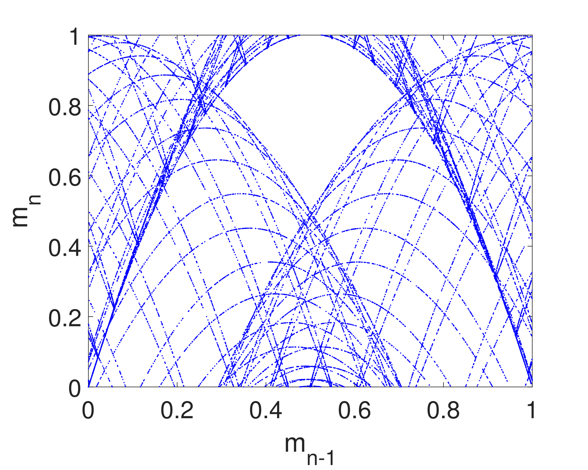
Figure 5: $(m_{(n-1)2},m_{n2})$ from the time series $M2(x_{(i-k1)2},x_{i2})$ considering two memory units.

If we analyze time series $M2=m_{02},m_{12},m_{22},\ldots$ with two memory units, for $\alpha=4$. The elements $m_{i2}$ of the time series $M2(x_{(i-k1)2},x_{i2})$ are obtained in the following way:

(13) $$m_{i2}=M2(x_{(i-k1)2},x_{i2})=x_{(i-k1)2}+x_{i2},\mbox{mod 1},$$

where $k1=5$. In the plot of $m_{(n-1)2}$ against $m_{n2}$, it is possible to distinguish that the time series $M2$ are generated with the logistic map. Figure 5 shows $(m_{(n-1)2},m_{n2})$ using two memory units. Because the length of the delay does not matter, the shape of the logistic map always remains, so it is necessary to consider more memory units.

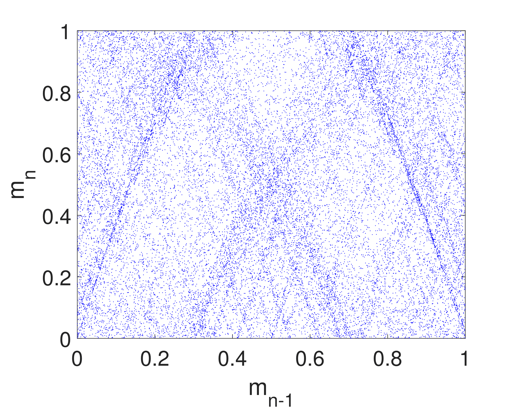
Figure 6: $(m_{(n-1)2},m_{n2})$ from the time series $M2(x_{(i-k2)2},x_{(i-k1)2},x_{i2})$ considering three memory units.

Now, if we consider three memory units to obtain the elements of the time series $M2(x_{(i-k2)2},x_{(i-k1)2},x_{i2})$ given as follows

(14) $$m_{i2}=M2(x_{(i-k2)2},x_{(i-k1)2},x_{i2})=x_{(i-k2)2}+x_{(i-k1)2}+x_{i2},\mbox{mod 1},$$

where $k1=10$ and $k2=5$. Now, for this case of three memory units, which are the minimum amount to obtain cloud of points in $(m_{(n-1)2},m_{n2})$, see Figure 6. The shape of the logistic map almost disappears, so three memory units are enough. The problem with considering more memory units has a computational price of information storage. For this reason two delays $k1$ and $k2$ and the present state of the time series of the logistic map are used. Also the lags must not be contiguous in order to avoid regular patterns which directly affect the test results.

It is considered different delays, i.e., $k_{2}=k^{\prime}_{2}=10$, $k_{1}=6$ and $k^{\prime}_{1}=5$ for both time series $M1$ and $M2$. Thus, these series are conformed by the sum of two delay states $x_{(i-10)1}$ and $x_{(i-5)1}$ with the actual state $x_{i1}$ of the orbit $x_{01},x_{11},x_{21},\ldots$, for $M1$. In the same way for $M2$, $x_{(i-10)2}$, $x_{(i-6)2}$ and $x_{i2}$ of the orbit $x_{02},x_{12},x_{22},\ldots$. The values of the time series are limited by the operation mod 1, this guarantees that $M1,M2\in[0,1)\subset\Re$. Explicitly $M1(x_{(i-10)1},x_{(i-5)1},x_{i1})$ and $M2(x_{(i-10)2},x_{(i-6)2},x_{i2})$ are expressed in the following way:

(15) $$m_{i1}=M1(x_{(i-10)1},x_{(i-5)1},x_{i1})=x_{(i-10)1}+x_{(i-5)1}+x_{i1},\mbox{mod 1},$$

(16) $$m_{i2}=M2(x_{(i-10)2},x_{(i-6)2},x_{i2})=x_{(i-10)2}+x_{(i-6)2}+x_{i2},\mbox{mod 1}.$$

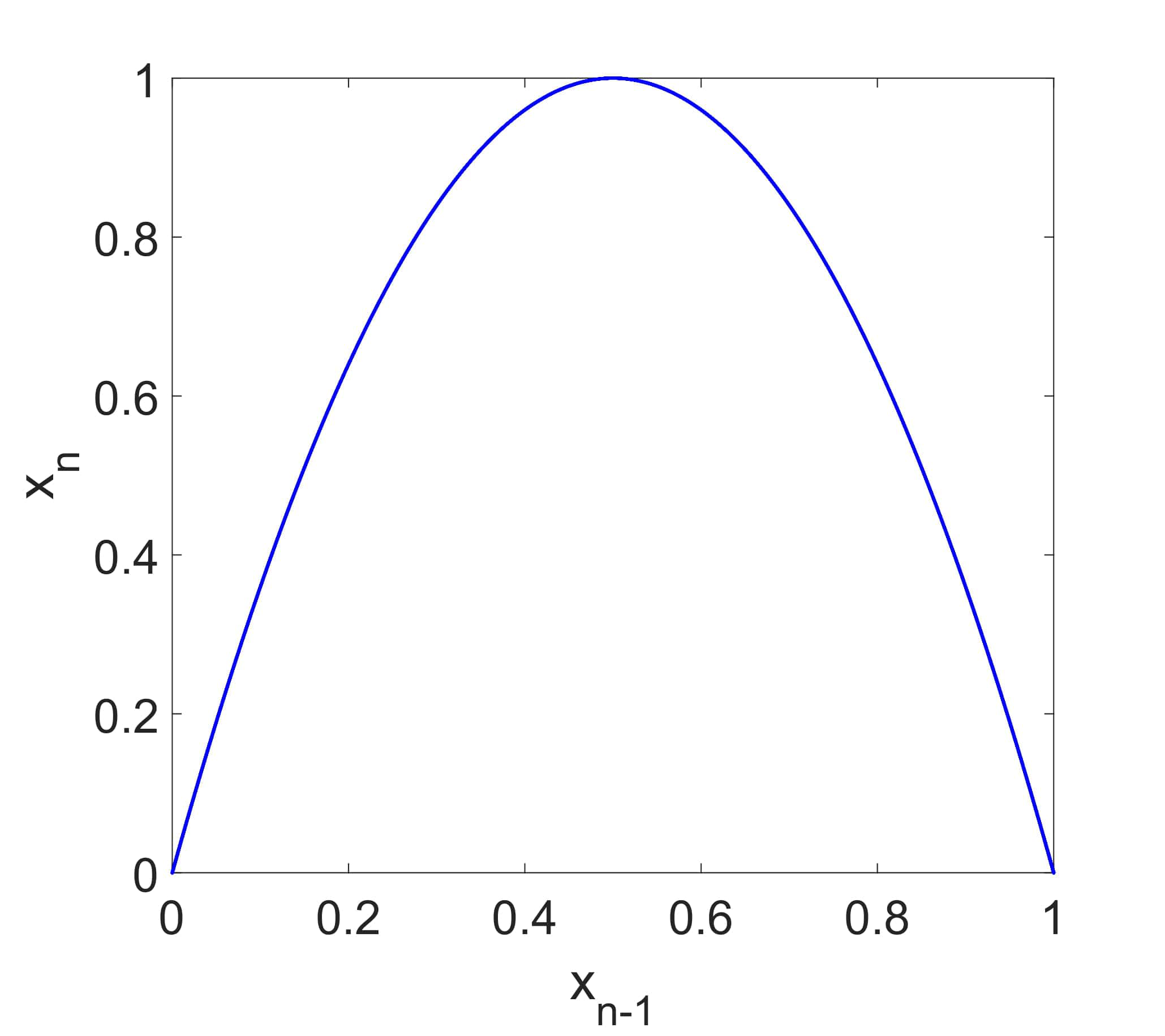
(a)

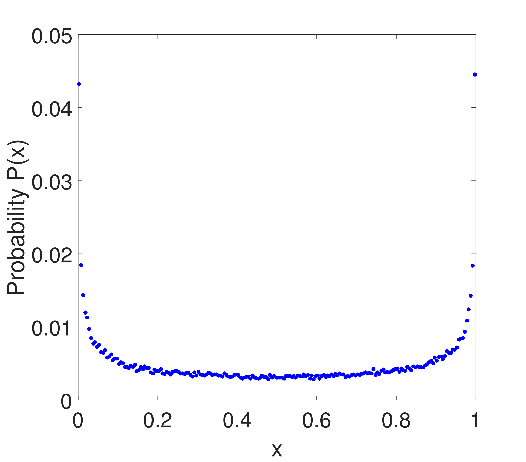
(b)

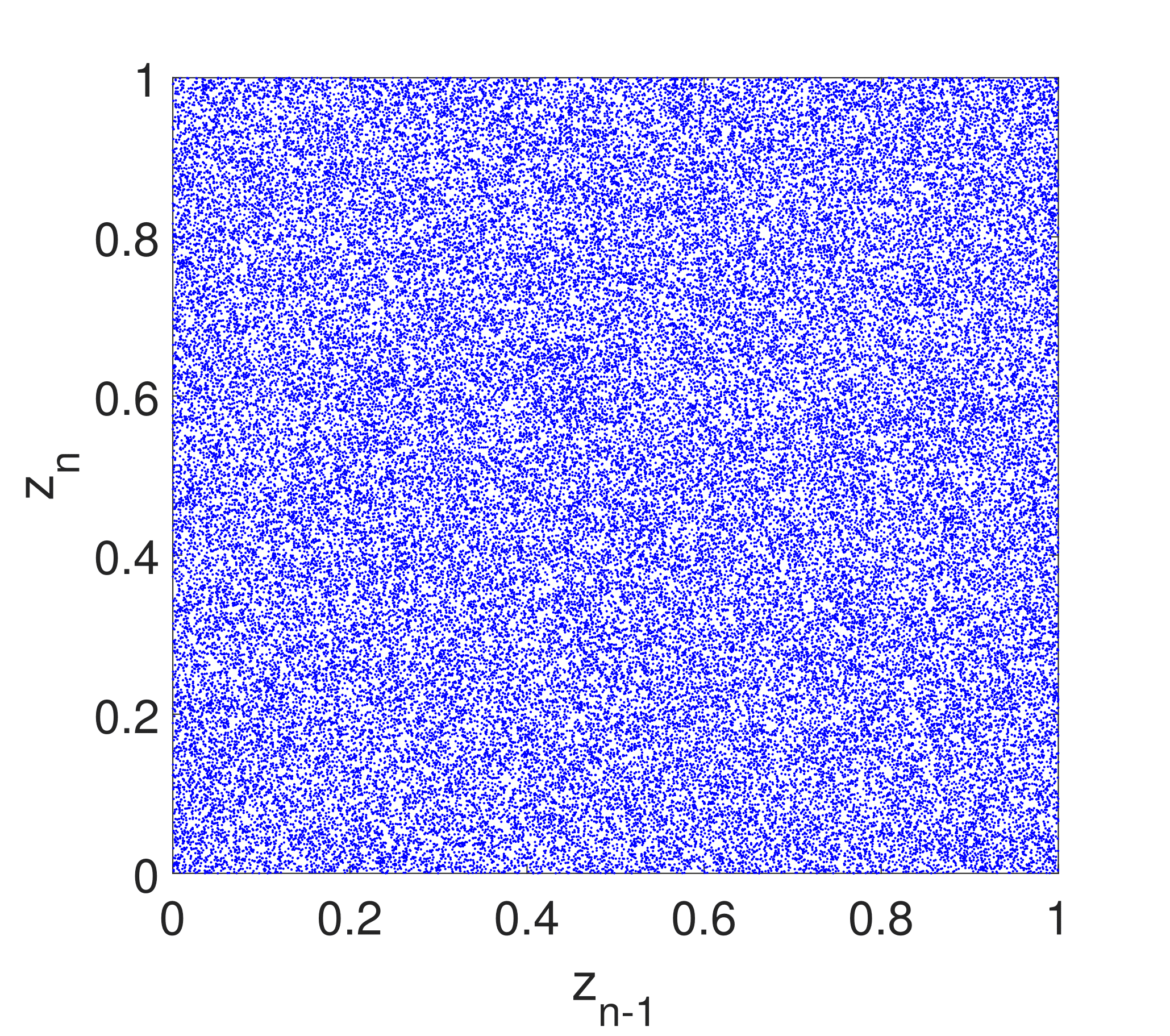
(c)

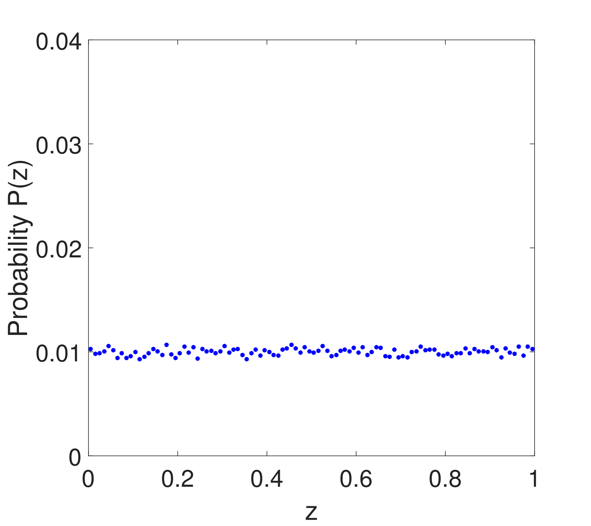
(d)

Figure 7: (a) Logistic map given by $x_{n}$ against $x_{n-1}$; (b) “U-shaped” probability distribution of the logistic map; (c) Delayed map given by $z_{n}$ against $z_{n-1}$; (d) Uniform probability distribution of the delayed map.

Finally, these time series $M1={m_{01},m_{11},m_{21},\ldots}$ and $M2={m_{02},m_{12},m_{22},\ldots}$ given by (15) and (16), respectively, are mixed and the operation mod 1 is applied again, this process generates a new time series $Z_{i}$ given as follows:

(17) $$Z_{i}=m_{i1}+m_{i2},\mbox{mod 1}.$$

From now on, Eq. (17) is referred as the delayed map. Note that $Z_{i}\in[0,1)\subset\Re$. The aim to use this approach is that with the combination of two time series with delays represented by $Z_{i}$, it is possible to dismiss the structure of the chaotic map used. For instance, the time series $x_{n}$ can reveal the map whether $x_{n}$ against $x_{n-1}$ is plotted as is shown in Figure 7 (a), the logistic map appears. In contrast, the time series $z_{n}$ can not reveal the map whether $z_{n}$ against $z_{n-1}$ is plotted as is shown in Figure 7 (c), the delays used are not reveled neither does the logistic map appear. As well as, this allows us to change the characteristic “U-shaped” probability distribution [28] by a uniform probability distribution in the obtained time series $x_{n}$ and $z_{n}$, see Figure 7 (b) and (d), respectively. This is an important characteristic that, in comparison with the chaos based schemes approach, makes easier the construction of S-box since all values has the same probability of occurrence in contrast with a single chaotic based schemes.

To obtain a binary time series $s$ useful for cryptosystems, it is constructed the symbolic dynamics of $Z_{i}$. So the elements of $s$ are binary numbers, i.e., $s_{i}(Z_{i})\in\{0,1\}$. One necessary requirement for the symbolic dynamic is to obtain zeros or ones with the same probability, thus the process for getting the binary series is as follows:

(18) $$s_{i}=\left\{\begin{array}[]{l}0,~{}~{}\mbox{for}~{}~{}0<Z_{i}\leq 0.5,\\ 1,~{}~{}\mbox{for}~{}~{}0.5<Z_{i}<1.\end{array}\right.$$

A CSPRNG based on a discrete dynamical system is given from equations (11) to (18).

4.1 The algorithm for s-box design via CSPRNG

In this subsection, we propose a novel design algorithm for the creation of $n\times n$ S-boxes based on CSPRNG. The steps of the algorithm are simple as shown below.

Step 1

Select initial conditions $x_{01}$ and $x_{02}$ for CSPRNG in order to generate the stream of bits $s_{0},s_{1},s_{2},\ldots$

Step 2

Generate the block sequence of $n$-bits each, $C_{0}=(s_{0},s_{1},\ldots,s_{n-1})$, $C_{1}=(s_{n},s_{n+1},\ldots,s_{2n-1})$, $C_{2}=(s_{2n},s_{2n+1},\ldots,s_{3n-1})$, $\ldots$

Step 3

Convert the blocks $C_{0},C_{1},C_{2},\ldots$ of $n$-bits to integer numbers $D_{0}$, $D_{1}$, $D_{2}$,$\ldots$.

Step 4

Discard the repeated elements $D$’s to select $2^{n}$ different values. The rule to discard an element is as follows: if $D_{i}=D_{j}$ with $i<j$ then discard $D_{j}$.

Step 5

Create the S-Box with the $2^{n}$ different elements of $D$’s.

Once the procedure is over, the proposed algorithm returns a $n\times n$ S-box with distinct $2^{n}$ values. Note that $D_{0}$ is the first element of the S-box, but the second element could be not $D_{1}$ if $D_{0}=D_{1}$. However, has been generated the enough $2^{n}$ elements to build the S-box. Each block $C$’s is comprised by $n$ bits, $s_{j},s_{j+1},\ldots,s_{j+n-1}$, which are related with the functions $f_{i}$, with $i=1,\ldots,n$.

For example, if $n=8$, $x_{01}=0.8147$, $x_{02}=0.9058$, $\alpha_{1}=4$ and $\alpha_{2}=-2$ then the $8\times 8$ S-Box is obtained in Table 2. This proposed substitution box has the properties of confusion and diffusion, which are of vital importance for the block ciphers.

64	46	150	174	220	26	233	224	148	170	143	247	225	212	90	124
44	204	59	61	43	121	129	2	109	164	103	249	16	237	27	35
216	184	81	213	161	169	89	199	140	38	239	48	163	193	21	147
222	217	70	196	195	192	234	41	47	15	14	42	98	190	186	36
242	51	60	87	24	104	189	55	118	111	231	120	8	226	7	141
85	9	73	101	3	197	12	66	82	110	65	25	165	176	80	181
125	31	218	74	68	52	149	95	182	19	112	5	136	79	214	34
158	50	188	137	28	191	155	84	105	126	92	179	162	152	200	0
171	142	240	203	88	160	32	202	99	18	100	97	145	53	194	93
245	119	185	20	235	123	134	139	128	116	173	76	17	132	209	135
83	168	57	56	223	30	91	4	22	122	102	221	208	131	71	86
39	114	252	10	172	201	177	77	94	246	54	175	183	108	156	45
219	210	40	130	113	153	13	166	58	23	253	215	238	33	198	248
229	227	96	206	107	144	67	254	115	167	244	106	180	157	255	241
207	243	228	187	49	78	251	37	62	1	205	117	29	178	75	236
11	250	146	6	151	69	138	133	72	232	211	127	159	63	154	230

Table 2: The S-box generated by proposed algorithm.

In the next section, is examined the performances of the proposed algorithm for the generation of S-Boxes to confirm their immunity especially against differential and linear cryptanalysis.

5 Performance test of S-box

In this section we compute six important and well-known cryptographic criteria of the $8\times 8$ S-boxes. Lastly, we present our results which are contrasted with some results presented in different published papers using other approaches.

5.1 Bijectivity criterion

The computed value of proposed S-box is the desired value of $2^{n-1}=128$, with $n=8$, according to the formula (2). So the bijectivity criterion is satisfied and the S-box proposed is a one-to-one, surjective and balance; which is a primary cryptographic criterion.

5.2 Nonlinearity Criterion

Nonlinearity is the major requirement of any S-box design due to ensure that an S-box is not a linear function between input vectors and output vectors. The nonlinearity symbolizes the degree of dissimilarity between the Boolean function $f$ and n-bit linear function $l$. If the function have high minimum Hamming distance is said to have high nonlinearity, i.e., by reducing the Walsh spectrum in (4). A S-box contains $n$ Boolean functions and the nonlinearity of each Boolean function must be calculated. The nonlinearities of the proposed S-box are $104$, $104$, $102$, $104$, $96$, $102$, $100$ and $102$, respectively. High nonlinearity ensures the strongest ability to resist powerful modern attacks such as linear cryptanalysis.

5.3 Strict Avalanche Criterion (SAC)

The Avalanche effect is used to indicate the randomness of an S-box when an input has a change. The matrix of the generated S-box can be found in Table 3. For the S-box proposed, it is obtained a maximum SAC equal to $0.5781$, the minimum is $0.3906$, and its average value $0.5012$ is close to the desired value $0.5$. Based on these results, it can be concluded that the S-box generated by our proposed method fulfills the property of SAC.

0.5781	0.4844	0.5000	0.4219	0.4844	0.5156	0.4063	0.5469
0.5156	0.5000	0.4688	0.5156	0.5469	0.3906	0.5469	0.4375
0.5469	0.5000	0.5000	0.5469	0.4063	0.5156	0.4531	0.5313
0.4531	0.5156	0.5000	0.4531	0.5313	0.5313	0.4844	0.4688
0.5156	0.5469	0.4844	0.5313	0.5313	0.5625	0.5625	0.5469
0.4063	0.4844	0.5000	0.4063	0.5625	0.5625	0.4844	0.5313
0.4219	0.4063	0.5313	0.5313	0.4219	0.5625	0.4844	0.4844
0.5469	0.5156	0.5469	0.5625	0.4531	0.5625	0.5781	0.4531

Table 3: SAC criterion result of the generated S-box.

5.4 Output Bits Independence Criterion (BIC)

The BIC criterion guarantees that there is no statistic pattern or dependency between output vectors. The BIC of the S-box generated by the proposed method is tested as described in Subsection 2.4, the results obtained are shown in Tables 4, 5 and 6. The mean value of BIC-nonlinearity is $103.8571$, the mean value of BIC-SAC is $0.5066$ and maximum value of DD is $8$ which indicates that S-box approximately satisfies the BIC criterion.

0	104	104	106	104	106	106	102
104	0	106	98	102	104	102	104
104	106	0	104	102	96	104	104
106	98	104	0	106	100	106	104
104	102	102	106	0	102	100	102
106	104	96	100	102	0	104	108
106	102	104	106	100	104	0	106
102	104	104	104	102	108	106	0

Table 4: BIC-nonlinearity criterion result of the generated S-box.

0	0.5020	0.5176	0.5137	0.5293	0.5098	0.4727	0.5059
0.5020	0	0.4980	0.4844	0.5039	0.5313	0.5156	0.5000
0.5176	0.4980	0	0.5039	0.4941	0.5313	0.5000	0.5020
0.5137	0.4844	0.5039	0	0.5117	0.4980	0.5020	0.5020
0.5293	0.5039	0.4941	0.5117	0	0.5234	0.5000	0.5137
0.5098	0.5313	0.5313	0.4980	0.5234	0	0.5039	0.5000
0.4727	0.5156	0.5000	0.5020	0.5000	0.5039	0	0.5156
0.5059	0.5000	0.5020	0.5020	0.5137	0.5000	0.5156	0

Table 5: BIC-SAC criterion result of the generated S-box.

0	2	6	2	4	6	4	6
2	0	2	2	2	2	4	2
6	2	0	6	8	2	6	4
2	2	6	0	4	2	8	4
4	2	8	4	0	2	0	2
6	2	2	2	2	0	2	8
4	4	6	8	0	2	0	0
6	2	4	4	2	8	0	0

Table 6: The DD of the generated S-box (BIC–SAC criterion).

5.5 Criterion of equiprobable Input/Output XOR Distribution

The equiprobable Input/Output XOR Distribution is a criterion which analyzes the effect in particular differences in input pairs of the resultant output pairs to discover the key bits. The idea is to find the high probability difference pairs for an S-Box under attack. The equiprobable input/output XOR distribution of generated S-box calculated by (12) is presented in Table 7. Maximal value of S-box generated by the proposed method is $5$, which indicates that our S-box satisfies bound for the equiprobable Input/Output XOR Distribution criterion.

4	3	3	4	3	3	3	3	4	3	3	3	3	3	4	4
3	3	4	3	3	4	3	3	4	3	3	4	4	4	4	3
4	3	4	3	4	4	3	3	3	3	3	3	3	4	3	3
4	3	3	3	4	4	4	4	3	4	5	4	3	2	3	3
5	4	4	3	3	3	4	4	4	3	5	3	3	3	3	3
3	3	3	4	4	3	5	4	3	3	3	5	5	3	3	3
3	3	3	3	3	4	4	3	3	3	4	3	3	2	3	3
3	2	3	3	3	4	3	3	3	3	3	4	3	3	3	3
3	3	3	5	5	3	3	4	3	4	3	2	5	3	3	3
3	3	3	4	3	4	3	3	3	4	3	3	4	3	4	3
4	3	4	3	2	3	3	4	3	3	3	3	3	4	3	3
3	4	3	3	3	3	3	3	3	4	3	3	3	3	4	4
3	3	3	3	3	4	3	3	2	4	3	3	4	4	3	3
4	3	4	3	4	4	3	4	4	3	4	4	3	3	3	3
3	4	3	3	3	3	3	3	3	4	4	3	3	3	3	3
3	3	3	5	4	5	4	3	3	5	3	3	4	3	5	-

Table 7: Equiprobable Input/Output XOR Distribution approach table for the generated S-box.

5.6 MELP criterion of the generated S-box

The MELP value is calculated via linear approximations to model nonlinear steps. The final goal is to recover the key bits or part of the key bits. MELP studies the statistical correlation between the input and the output. This criterion of proposed S-Box is computed according to equation (9) and the average value is $0.0176$.

5.7 Comparative results

In this section a performance comparison of the S-box created using the algorithm described in Subsection 4.1 is presented. In the Table 8 the criteria values for our S-box and a set of widely known boxes (standard and chaos based S-box) are shown. From this Table 8, it can be seen that the generated S-box fulfills the most important condition, bijectivity, and accomplish a good similarity to the rest of the test values expected [3, 7, 10, 29, 30, 31, 32, 33, 34, 35, 36]. Mainly it shows better performance in the tests related to attacks (MELP and equiprobable Input/Output XOR Distribution). Also is a methodology based on a system with simple operations that generates sequences with complex behavior.

	Bijective	Nonlinearity			SAC			BIC			I/O XOR	MELP
		min	max	avg	min	max	avg	SAC	Nonlinearity	DD
Skipjack S-Box [37]	123	100	108	105.1250	0.3906	0.5938	0.5027	0.5003	104.03	109	0.0469	0.0137
APA S-Box [29]	128	112	112	112	0.4375	0.5625	0.5007	0.4997	112	112	0.0156	0.0039
Gray S-Box [30]	128	112	112	112	0.4375	0.5625	0.4998	0.5026	112	112	0.0156	0.0039
AES S-Box [31]	128	112	112	112	0.4531	0.5625	0.5049	0.5046	112	112	0.0156	0.0039
Ref. [3]	128	98	107	103.25	0.3828	0.5938	0.5059	0.5033	104.21	108	0.0469	0.0166
Ref. [32]	129	103	109	104.875	0.3984	0.5703	0.4966	0.5044	102.96	109	0.0391	0.0176
Ref. [33]	128	96	106	103	0.3906	0.6250	0.5039	0.5010	100.35	106	0.5000	0.0220
Ref. [34]	128	112	112	112	0.4219	0.5469	0.5115	0.4982	108.71	112	0.0313	0.0120
Ref. [7]	128	102	108	105.25	0.4375	0.5781	0.5056	0.5019	103.78	108	0.0391	0.0244
Ref. [10]	128	104	110	106.25	0.4219	0.5938	0.5039	0.5059	103.35	108	0.0391	0.0198
Ref. [35]	128	102	108	106	0.4219	0.5938	0.5002	0.5016	104.42	108	0.0391	0.0220
Ref. [36]-1	128	106	108	106.75	0.3906	0.6094	0.4941	0.5013	104.28	108	0.0391	0.0156
Ref. [36]-2	128	106	108	106.75	0.4063	0.5938	0.4971	0.5008	102.92	106	0.0391	0.0198
The proposed S-box	128	96	104	101.75	0.3906	0.5781	0.5012	0.5066	103.42	108	0.0391	0.0176

Table 8: Comparison of recent chaos-base designed S-Boxes and S-boxes used in typical block ciphers.

6 Dynamical generation of S-boxes and its application

The Alberti cipher was one of the first polyalphabetic ciphers where the principle is based on substitution, using multiple substitution alphabets such that the output has a uniform distribution. Taking this idea of polyalphabetic ciphers, it is presented an application of dynamical generation of S-boxes, i.e., a particular intensity of a pixel given can be substituted by different intensities in the same round. Usually an S-box is used to substitute all the pixels of an image of size $p\times q$ in the same way. The idea of polyalphabetic ciphers is to use a dynamical S-box to achieve this aim looking for a uniform distribution. For instance, our dynamical S-box belongs to a class of S-boxes given by $p$ elements (S-boxes) generated by the algorithm presented in the Subsection 4.1. The approach to get uniform distribution is given by applying dynamical S-box which changes with each pixel row, i.e., the dynamical S-box is modified with a different S-box. Figure 8 shows the original Lena image and the codified Lena image alone with their gray scale pixels distribution.

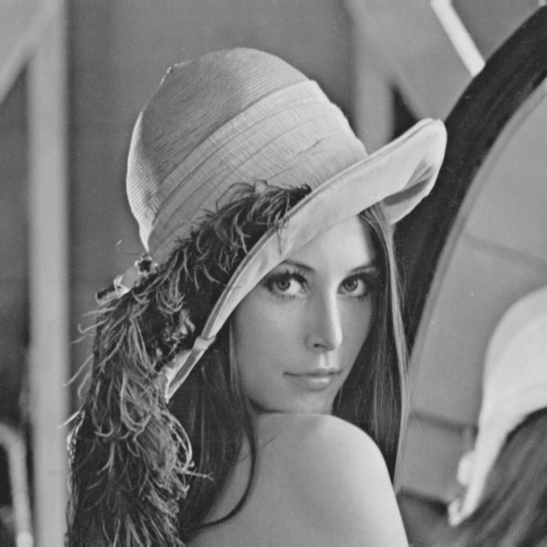
(a)

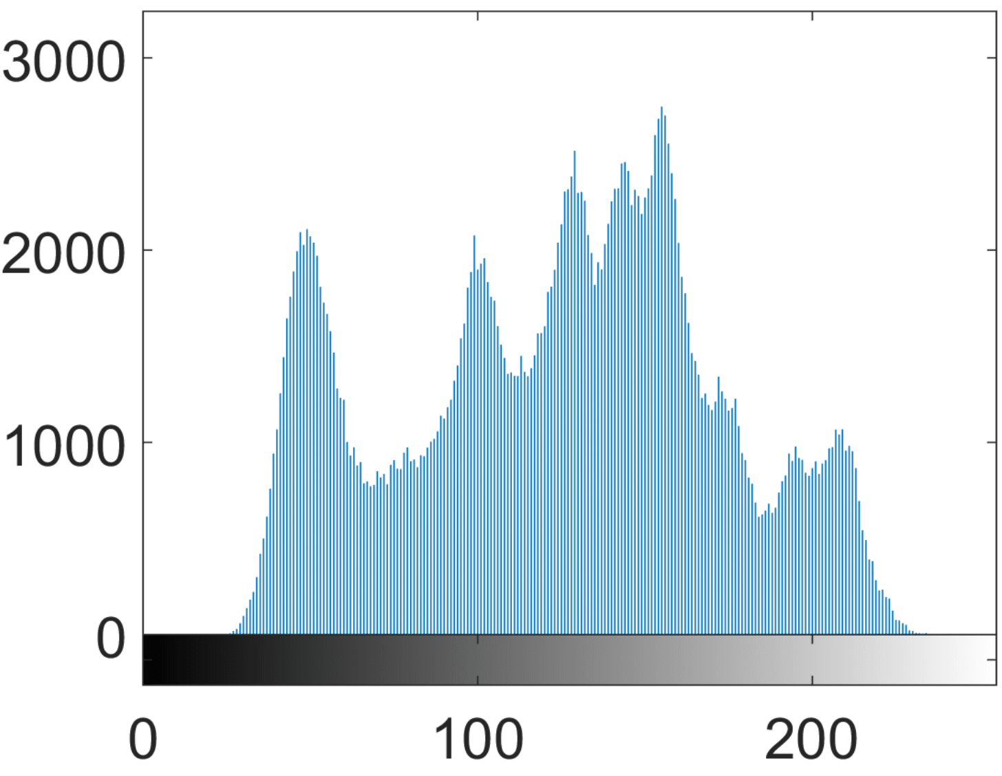
(b)

(c)

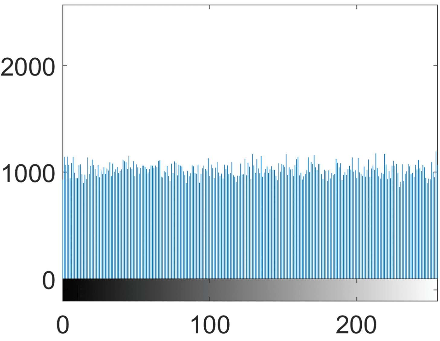
(d)

Figure 8: Plain image of Lena, encrypted image and their histograms.

In crypthography a uniform distribution is always desired, since this property was achieved by simple substitution of our S-boxes, a good result is spected for a full cryptographic algorithm based on our S-boxes.

It is important to point out that this is not an encryption algorithm, but a simple and useful approach intended to bring to light possible applications of our dynamical S-boxes.

7 Concluding remarks

In this work, a simple algorithm was proposed to generate $n\times n$ S-boxes by means of using a pseudo-random bit generator (PRBG) based on two lag time series of the logistic map. The mixed of this two time series favors a uniform distribution in addition to hide the chaotic map used. To evaluate performance of the proposed S-box, several statistical tests were carried out. The results of numerical analysis of these cryptographic strong S-box generated by the algorithm have also shown that all criteria for a good S-box were fulfilled and with high immunity to resist differential cryptanalysis and linear cryptanalysis. The performance test result was compared with other S-Boxes which were reported in the literature. Finally, an application based on simple and useful approach to bring uniform distribution was presented.

References

- [1] C. E. Shannon, Communication theory of secrecy systems, Bell System Technical Journal 28 (4) (1949) 656–715.
- [2] C. Adams, S. Tavares, The structured design of cryptographically good s-boxes, Journal of Cryptology 3 (1) (1990) 27–41.
- [3] G. Jakimoski, L. Kocarev, Chaos and cryptography: block encryption ciphers based on chaotic maps, IEEE Transactions on Circuits and Systems I: Fundamental Theory and Applications 48 (2) (2001) 163–169.
- [4] G. Chen, A novel heuristic method for obtaining s-boxes, Chaos, Solitons & Fractals 36 (4) (2008) 1028 – 1036.
- [5] Y. Wang, K.-W. Wong, X. Liao, T. Xiang, A block cipher with dynamic s-boxes based on tent map, Communications in Nonlinear Science and Numerical Simulation 14 (7) (2009) 3089 – 3099.
- [6] D. Lambić, A novel method of s-box design based on chaotic map and composition method, Chaos, Solitons & Fractals 58 (2014) 16 – 21.
- [7] A. Belazi, M. Khan, A. A. A. El-Latif, S. Belghith, Efficient cryptosystem approaches: S-boxes and permutation–substitution-based encryption, Nonlinear Dynamics 87 (1) (2017) 337–361.
- [8] F. Özkaynak, A. B. Özer, A method for designing strong s-boxes based on chaotic Lorenz system, Physics Letters A 374 (36) (2010) 3733 – 3738.
- [9] G. Liu, W. Yang, W. Liu, Y. Dai, Designing s-boxes based on 3-d four-wing autonomous chaotic system, Nonlinear Dynamics 82 (4) (2015) 1867–1877.
- [10] Ü. Çavuşoğlu, A. Zengin, I. Pehlivan, S. Kaçar, A novel approach for strong s-box generation algorithm design based on chaotic scaled Zhongtang system, Nonlinear Dynamics 87 (2) (2017) 1081–1094.
- [11] R. Guesmi, M. A. B. Farah, A. Kachouri, M. Samet, A novel design of chaos based s-boxes using genetic algorithm techniques, in: 2014 IEEE/ACS 11th International Conference on Computer Systems and Applications (AICCSA), 2014, pp. 678–684.
- [12] Y. Tian, Z. Lu, S-box: Six-dimensional compound hyperchaotic map and artificial bee colony algorithm, Journal of Systems Engineering and Electronics 27 (1) (2016) 232–241.
- [13] G. Alvarez, S. Li, Some basic cryptographic requirements for chaos-based cryptosystems, International Journal of Bifurcation and Chaos 16 (08) (2006) 2129–2151.
- [14] F. Özkaynak, S. Yavuz, Designing chaotic s-boxes based on time-delay chaotic system, Nonlinear Dynamics 74 (3) (2013) 551–557.
- [15] Y. Zhou, L. Bao, C. P. Chen, Image encryption using a new parametric switching chaotic system, Signal Processing 93 (11) (2013) 3039 – 3052.
- [16] M. García-Martínez, E. Campos-Cantón, Pseudo-random bit generator based on lag time series, International Journal of Modern Physics C 25 (04) (2014) 1350105.
- [17] D. Souravliasa, K. E. Parsopoulos, G. C. Meletiou, Designing bijective s-boxes using algorithm portfolios with limitedtime budgets, Applied Soft Computing 59 (1) (2017) 475–486.
- [18] C. Adams, S. Tavares, Good s-boxes are easy to find, in: G. Brassard (Ed.), Advances in Cryptology — CRYPTO’ 89 Proceedings, Springer New York, New York, NY, 1990, pp. 612–615.
- [19] Y. Tian, Z. Lu, Chaotic s-box: Intertwining logistic map and bacterial foraging optimization, Mathematical Problems in Engineering (2017) 1–11.
- [20] W. Millan, How to improve the nonlinearity of bijective s-boxes, in: C. Boyd, E. Dawson (Eds.), Information Security and Privacy, Springer Berlin Heidelberg, Berlin, Heidelberg, 1998, pp. 181–192.
- [21] A. F. Webster, S. E. Tavares, On the design of s-boxes, in: H. C. Williams (Ed.), Advances in Cryptology — CRYPTO ’85 Proceedings, Springer Berlin Heidelberg, Berlin, Heidelberg, 1986, pp. 523–534.
- [22] E. Biham, A. Shamir, Differential cryptanalysis of DES-like cryptosystems, in: A. J. Menezes, S. A. Vanstone (Eds.), Advances in Cryptology-CRYPT0’ 90, Springer Berlin Heidelberg, Berlin, Heidelberg, 1991, pp. 2–21.
- [23] R. M. May, Simple mathematical models with very complicated dynamics, Nature 261 (5560) (1976) 459.
- [24] D. S. Dendrinos, M. Sonis, Socio-spatial stocks and antistocks; the logistic map in real space, The Annals of Regional Science 27 (4) (1993) 297–313.
- [25] R. L. Devaney, An introduction to chaotic dynamical systems, Westview Press.
- [26] C. Li, G. Chen, Estimating the lyapunov exponents of discrete systems, Chaos 14 (2) (2004) 343–346.
- [27] C. Yang, C. Q. Wu, P. Zhang, Estimation of lyapunov exponents from a time series for n-dimensional state space using nonlinear mapping, Nonlinear Dynamics 69 (4) (2012) 1493–1507.
- [28] J. Urías, E. Campos, N. F. Rulkov, Random Finite Approximations of Chaotic Maps, Springer, New York, NY, 2006, pp. 231–242.
- [29] L. Cui, Y. Cao, A new s-box structure named affine-power-affine, International Journal of Innovative Computing, Information and Control 3 (3) (2007) 751–759.
- [30] M. T. Tran, D. K. Bui, A. D. Duong, Gray s-box for advanced encryption standard, in: 2008 International Conference on Computational Intelligence and Security, Vol. 1, IEEE, 2008, pp. 253–258.
- [31] J. Daemen, V. Rijmen, AES proposal: Rijndael, available: http://csrc.nist.gov/archive/aes/rijndael/Rijndael-ammended.pdf (1999).
- [32] G. Tang, X. Liao, A method for designing dynamical s-boxes based on discretized chaotic map, Chaos, Solitons & Fractals 23 (5) (2005) 1901–1909.
- [33] M. Khan, T. Shah, H. Mahmood, M. A. Gondal, I. Hussain, A novel technique for the construction of strong s-boxes based on chaotic Lorenz systems, Nonlinear Dynamics 70 (3) (2012) 2303–2311.
- [34] A. Belazi, A. A. A. El-Latif, A.-V. Diaconu, R. Rhouma, S. Belghith, Chaos-based partial image encryption scheme based on linear fractional and lifting wavelet transforms, Optics and Lasers in Engineering 88 (2017) 37–50.
- [35] F. ul Islam, G. Liu, Designing s-box based on 4D-4wing hyperchaotic system, 3D Research 8 (1) (2017) 1–9.
- [36] F. Özkaynak, Construction of robust substitution boxes based on chaotic systems, Neural Computing and Applications (2017) 1–10.
- [37] I. Hussain, T. Shah, M. A. Gondal, Y. Wang, Analyses of SKIPJACK s-box, World Appl. Sci. J. 13 (11) (2011) 2385–2388.