Large thermal anisotropy in monoclinic niobium trisulfide: A thermal expansion tensor study

Abstract

We present a method based on the Grüneisen formalism to calculate the thermal expansion coefficient (TEC) tensor that is applicable to any crystal system, where the number of phonon calculations associated with different deformations scales linearly with the number of lattice parameters. Compared to simple high-symmetry systems such as cubic or hexagonal systems, a proper consideration of low-symmetry systems such as monoclinic or triclinic crystals demands a clear distinction between the TEC tensor and the lattice-parameter TECs along the crystallographic directions. The latter is more complicated and it involves integrating the equations of motion for the primitive lattice vectors, with input from the TEC tensor. A first-principles study of the TEC is carried out for the first time on a monoclinc crystal, where we unveil high TEC anisotropies in a recently reported monoclinic phase of niobium trisulfide (NbS₃) crystal with a relatively large primitive cell (32 atoms per cell) using density-functional theory. We find the occurrence of a negative TEC tensor component is largely due to the mechanical property rather than the anharmonic effect, contrary to the common belief. Our theoretical treatment of the monoclinic system with a single off-diagonal tensor element could be routinely generalized to any crystal system, including the lowest-symmetry triclinic system with three off-diagonal tensor elements.

I Introduction

Thermal expansion of materials is a direct manifestation of the anharmonic effects inherent in a solid. A good understanding of the phonon dynamics affected by temperature-induced crystal deformations is often required for improved device applicationsGoodwin et al. (2008); Lin et al. (2011); Kim et al. (2012). So far ab initio studies of anharmonic effects in high-symmetry crystals such as cubic and hexagonal systems have been carried out via the quasiharmonic approximation (QHA) Mounet and Marzari (2005); Stoffel et al. (2015). The application of QHA on low-symmetry crystals is extremely challenging because many sets of time-consuming phonon calculations are required to search for the free energy minimum in a much larger lattice-parameter space, which may explain why, to the best of our knowledge, no studies have been carried out on, say, a monoclinic system. Even if a direct free energy minimization via QHA could be carried out, it may be still difficult to understand the underlying physics without interpreting the phonon frequency shifts due to a crystal deformation, phonon density of states, mechanical properties such as elastic constants and elastic compliances, and heat capacities. Since many technologically important materials are also found in low crystal symmetries, e.g., hybrid perovskitesCalabrese et al. (1991); Du et al. (2017); Giovanni et al. (2018) and ceramicsZhao and Vanderbilt (2002); Haggerty et al. (2014), it is desirable to be able to address the anharmonicity in these materials through other means. Recently, the Grüneisen approach has between applied to high-symmetry crystal systems and good agreements between theoretical predictions and experimental results Ding and Xiao (2015); Liu et al. (2017); Gan and Lee (2018). In this work, we extend the utility of the Grüneisen formalismGrüneisen (1926); Schelling and Keblinski (2003) to handle low-symmetry crystals. As will be shown later in this paper, dealing with low-symmetry crystals requires a clear distinction to be made between the thermal expansion coefficient (TEC) tensor and the lattice-parameter TECs. These two concepts, unfortunately, coincide with each other in high-symmetry crystals such as the cubic crystal. Other methods to calculate TECs are the vibrational self-consistent-field methodMonserrat et al. (2013) and the self-consistent quasiharmonic approximationHuang et al. (2016). We should note that the knowledge of the third-order interatomic force constantsBarron and Klein (1974); Shiomi et al. (2011) can be used directly to calculate the Grüneisen parameters for the evaluation of TECs. Another recent work Lee and Gan (2017) outlines a reverse process where numerically computed Grüneisen parameters could be used to extract the third-order interatomic force constants for the calculations of thermal conductivity.

The monoclinic NbS₃-IVBloodgood et al. (2018) (with four lattice parameters) belongs to a class of semiconducting transition metal chalcogenides. Transition metal chalcogenides have received attention due to their potential to replace traditional semiconductor technologies. They have been investigated for their electronic and optical properties, and their potential use in electronic devicesRibeiro et al. (2018). The extensive interest in metal chalcogenidesZhao et al. (2011); Chong et al. (2014) arises from the low-dimensionality of the structure. As a prototypical example of metal trichalcogenides (MX₃), niobium trisulfide (NbS₃) comprises of [NbS₆] units, where the sulfur atoms are arranged in a triangular prism around a central Nb atomvan Smaalen (1988). Neighboring trigonal prisms share a triangle face, thus fusing individual units to form an infinite chain along the $b$ axis. The chains are held together by additional covalent bonds to form bilayer sheets which interact via van der Waals forces. Experimentally, NbS₃ has been found to crystallize in six polymorphs: I, II, III, IV, V and a high-pressure phase. The first polymorph of NbS₃, NbS₃-I, first identified using single crystal x-ray diffractionJellinek (1960); Rijnsdorp and Jellinek (1978), belongs to space group $P\bar{1}$. Using electron diffraction studies, NbS₃-II was the second polymorph to be identified, although the structure remains unknown to date. Both NbS₃-II and NbS₃-III exhibit charge density wave (CDW) transitionsZettl et al. (1982); Zybtsev et al. (2017). Recently, Bloodgood et al.Bloodgood et al. (2018) reported the synthesis of new monoclinic polymorphs of NbS₃, where structural information was obtained via single crystal x-ray diffraction, electron microscopy, and Raman spectroscopy studiesBloodgood et al. (2018). The new polymorphs, NbS₃-IV and NbS₃-V, were found to crystallize in the space groups $P12_{1}/c1$ and $P12_{1}/m1$, respectively. Presently, first-principles studies of the anharmonic effects that account for thermal expansion are lacking for these compounds.

The outline of this paper is as follows: Sec. II.1 discusses the concepts of a TEC tensor and lattice-parameter TECs and the distinction between them. Sec. II.2 presents the Grüneisen formalism for the computation of the TEC tensors. For efficient implementation and a good physical interpretation, Sec. II.3 shows how the tensorial expression can be turned into a simple matrix expression. Sec. II.4 discusses the deformations that are to be applied to the crystal for the calculations of elastic constants and Grüneisen parameters. The procedure for elastic constant calculations is outlined in Sec. II.5 where we observe that all required elastic constants for the TEC calculations can be obtained from symmetry-preserving deformations. In Sec. II.6, we describe how the lattice-parameter TECs may be obtained from a TEC tensor by solving a set of coupled differential equations. The reverse of this process is presented in Appendix A. The results are presented in Sec. III. Finally Sec. IV contains the conclusions.

II Methodology

II.1 TEC tensor versus lattice-parameter TECs

Thermal expansion of a crystal can generally be described by the thermal expansion coefficient (TEC) tensor with components $\alpha_{ij}(T)$ that depend on temperature $T$. When the temperature changes, the crystal will change its shape according to a strain tensor $\epsilon_{ij}$ induced by the TEC tensor where

$$\frac{d\epsilon_{ij}}{dT}=\alpha_{ij}(T)$$ (1)

In three dimensions, the most general $\alpha_{ij}(T)$ is a $3\times 3$ symmetric tensor with six independent parameters. For a cubic crystal, it turns out that $\alpha_{11}(T)=\alpha_{22}(T)=\alpha_{33}(T)$ while all crossed terms $\alpha_{ij}(T)=0$, $i\neq j$, which means that only one independent parameter is needed to describe the TEC. Also it does not matter how the cubic crystal is oriented in space since the expansion is isotropic. Specifically, the TEC tensor components $\alpha_{ii}(T)$ are all equal for $i=1,2,3$, and they coincide with the meaning of the $a$ lattice-parameter TEC, denoted by $\alpha_{a}(T)=\frac{1}{a(T)}{\frac{da(T)}{dT}}$ for the cubic crystal where $a$ is the lattice constant. In another example, the hexagonal crystal is described by two independent TEC tensor components $\alpha_{a}(T)=\alpha_{11}(T)=\alpha_{22}(T)$, and $\alpha_{c}(T)=\alpha_{33}(T)$ where we must tacitly assume that the $c$ axis is pointing in the $z$ Cartesian direction. However, for a low-symmetry monoclinic crystal (with lattice parameters $a\neq b\neq c$ and $\beta\neq 90^{\circ}$), the matter becomes slightly more complicated. It is usually convenient to choose a crystal orientation where the $b$ lattice parameter is parallel to the $y$ Cartesian direction (the so-called ‘unique axis $b$’ in Ref. [Hahn, Ed.]). Symmetry considerations and Neumann’s principle dictates that the TEC tensor of a monoclinic crystal is of the following formSchlenker et al. (1975); Nye (1985)

$$\begin{pmatrix}\alpha_{11}&0&\alpha_{31}\\ 0&\alpha_{22}&0\\ \alpha_{31}&0&\alpha_{33}\end{pmatrix}$$ (2)

Here, there are four independent components of the TEC tensor. Similar to the basic definition of the lattice-parameter TEC $\alpha_{a}(T)$ for a cubic crystal, we define a lattice-parameter TEC of a monoclinic crystal according to

$$\alpha_{\ell}(T)=\frac{1}{\ell(T)}\frac{d\ell(T)}{dT}$$ (3)

where $\ell$ equals to one of the monoclinic lattice parameters $a$, $b$, $c$, and $\beta$. Since the $b$ axis is unique by choice, the $\alpha_{22}(T)$ component is decoupled from the other three components and coincides with the $b$ lattice-parameter TEC, where $\alpha_{b}(T)=\alpha_{22}(T)$. With a ‘unique axis b’ choice, it is still necessary to clearly state the crystal orientation before reporting the other three TEC tensor components $\alpha_{11}(T)$, $\alpha_{33}(T)$, and $\alpha_{31}(T)$. Unless the $a$ lattice parameter happens to be aligned along the $x$ Cartesian axis, $\alpha_{11}(T)$ is not same as the lattice-parameter TEC for $a$. It is then apparent that the temperature dependence of $a$, $c$, and $\beta$ collectively depend on $\alpha_{11}(T)$, $\alpha_{33}(T)$, and $\alpha_{31}(T)$, and vice versa. In Sec. II.6 and Appendix A we derive the relations between these two TEC descriptions. Throughout this work, we assume the orientation of a monoclinic crystal in equilibrium at $T=0$ K is as follows:

$${\boldsymbol{a}}=a{\boldsymbol{i}},$$

$${\boldsymbol{b}}=b{\boldsymbol{j}},$$

$${\boldsymbol{c}}=c\cos\beta{\boldsymbol{i}}+c\sin\beta{\boldsymbol{k}}.$$ (4)

The Cartesian unit vectors are ${\boldsymbol{i}}$, ${\boldsymbol{j}}$, and ${\boldsymbol{k}}$. It is important to note that for $T>0$ K, ${\boldsymbol{a}}$ may have a nonzero component along ${\boldsymbol{k}}$ due to presence of the off-diagonal $\alpha_{31}(T)$ component.

We shall now comment on the nonuniqueness of the choice of $a$, $c$, and $\beta$ of a monoclinic primitive cell, even within a ‘unique axis $b$’ choice. With the specific choice adopted in Eq. 4, we may derive from it a second set of primitive lattice vectors such as

$${\boldsymbol{a}}^{\prime}={\boldsymbol{a}}=a{\boldsymbol{i}},$$

$${\boldsymbol{b}}^{\prime}={\boldsymbol{b}}=b{\boldsymbol{j}},$$

$${\boldsymbol{c}}^{\prime}={\boldsymbol{c}}-{\boldsymbol{a}}=c^{\prime}\cos\beta^{\prime}{\boldsymbol{i}}+c^{\prime}\sin\beta^{\prime}{\boldsymbol{k}},$$ (5)

This will in general have the consequence that $\alpha_{c^{\prime}}\neq\alpha_{c}$ and $\alpha_{\beta^{\prime}}\neq\alpha_{\beta}$. We shall see the effect of such a choice on the results in Section III.

We may calculate the volumetric TEC $\alpha_{v}$ (with suppressed $T$ dependence for clarity) from

$$\alpha_{v}=\left|\begin{array}[]{ccc}\ 1+\alpha_{11}&0&\alpha_{31}\\ 0&1+\alpha_{22}&0\\ \alpha_{31}&0&1+\alpha_{33}\end{array}\right|-1$$ (6)

The same $\alpha_{v}$ can also be calculated from the lattice-parameter TECs where

$$\alpha_{v}=\alpha_{a}+\alpha_{b}+\alpha_{c}+\frac{\beta\cos\beta}{\sin\beta}\alpha_{\beta}$$ (7)

This can be derived from the expression for the volume of the primitive cell $\Omega$ where $\Omega=abc\sin\beta$.

II.2 Grüneisen formalism

The TEC tensor components $\alpha_{ij}(T)$ for any crystal at temperature $T$ may be calculated from first-principles via a Grüneisen formalismGrüneisen (1926); Schelling and Keblinski (2003) expressed in a tensorial form:

$$\alpha_{ij}(T)=\frac{1}{\Omega}\sum_{k=1}^{3}\sum_{l=1}^{3}S_{ijkl}I_{kl}(T)$$ (8)

The elastic compliance tensor and equilibrium volume of the primitive cell are denoted by $S_{ijkl}$ and $\Omega$, respectively.

Central to the Grüneisen formalism are the integrated quantities $I_{ij}(T)$ given by

$$I_{ij}(T)=\frac{\Omega}{\left(2\pi\right)^{3}}\sum_{\lambda}\int_{\rm BZ}d{\boldsymbol{q}}\,\gamma_{ij,\lambda{\boldsymbol{q}}}\,c(\nu_{\lambda{\boldsymbol{q}}},T)$$ (9)

Here $\nu_{\lambda{\boldsymbol{q}}}$ denotes the frequency of a phonon mode with mode index $\lambda$ and wave-vector ${\boldsymbol{q}}$. The heat capacity of a phonon mode of frequency $\nu$ is given by $c(\nu,T)=k_{{\scriptscriptstyle B}}(r/\sinh r)^{2}$, with $r=h\nu/2k_{{\scriptscriptstyle B}}T$, where $h$ and $k_{{\scriptscriptstyle B}}$ are the Planck and Boltzmann constants, respectively. The bandstructure-like deformation-dependent Grüneisen parameter is defined by

$$\gamma_{ij,\lambda{\boldsymbol{q}}}=-\frac{1}{\nu_{\lambda{\boldsymbol{q}}}}\frac{\partial\nu_{\lambda{\boldsymbol{q}}}}{\partial\epsilon_{ij}}$$ (10)

which measures the fractional change in phonon mode frequency with respect to a small strain $\epsilon_{ij}$ applied to the crystal. Phonon frequencies may be calculated accurately either from a density-functional perturbation theory (DFPT) approachBaroni et al. (2001) or a supercell force-constant methodKresse et al. (1995); Ackland et al. (1997); Alfè (2009). The Grüneisen parameters are calculated based on Eq. 10 from phonon frequency shifts using a central-difference scheme with the help of changes in the dynamical matrices and a perturbation theoryGan et al. (2015). In this work, we apply strains of $\epsilon=\pm 0.01$ for all deformations to determine the Grüneisen parameters.

The integrated quantity $I_{ij}(T)$ in Eq. 9 is seen as an integral over the Brillouin zone (BZ) of the product of the mode-dependent heat capacities and mode-dependent Grüneisen parameters. It can also be written as an integral over the phonon frequencies

$$I_{ij}(T)=\int_{\nu_{min}}^{\nu_{max}}d\nu\ \Gamma_{ij}(\nu)c(\nu,T)$$ (11)

where $\nu_{min}$ ($\nu_{max}$) is the minimum (maximum) frequency in the phonon spectrum. Here we have introduced a quantity called the density of the phonon states weighted by the Grüneisen parameters

$$\Gamma_{ij}(\nu)=\frac{\Omega}{\left(2\pi\right)^{3}}\sum_{\lambda}\int_{\rm BZ}d{\boldsymbol{q}}\ \gamma_{ij,\lambda{\boldsymbol{q}}}\delta(\nu-\nu_{\lambda{\boldsymbol{q}}})$$ (12)

With the definition in Eq. 12, we turn the direct summation in Eq. 9 into an integral given in Eq. 11 involving the two quantities $c(\nu,T)$, which has a form that is easily understood, and $\Gamma_{ij}(\nu)$, which captures the net effect of anharmonicities of all phonon modes with the same frequency $\nu$.

II.3 Compact matrix expression

We find it convenient to use the analogy of the strain-stress relationshipNye (1985) $\epsilon_{i}=S_{ij}\sigma_{j}$ to cast Eq. 8 into

$$\alpha_{i}(T)=\frac{1}{\Omega}S_{ij}I_{j}(T)$$ (13)

with the prescription

$$\begin{pmatrix}\alpha_{11}(T)&\alpha_{12}(T)&\alpha_{31}(T)\\ \alpha_{12}(T)&\alpha_{22}(T)&\alpha_{23}(T)\\ \alpha_{31}(T)&\alpha_{23}(T)&\alpha_{33}(T)\end{pmatrix}\rightarrow\begin{pmatrix}\alpha_{1}(T)&{\frac{1}{2}}\alpha_{6}(T)&{\frac{1}{2}}\alpha_{5}(T)\\ {\frac{1}{2}}\alpha_{6}(T)&\alpha_{2}(T)&{\frac{1}{2}}\alpha_{4}(T)\\ {\frac{1}{2}}\alpha_{5}(T)&{\frac{1}{2}}\alpha_{4}(T)&\alpha_{3}(T)\end{pmatrix}$$ (14)

and

$$\begin{pmatrix}I_{11}(T)&I_{12}(T)&I_{31}(T)\\ I_{12}(T)&I_{22}(T)&I_{23}(T)\\ I_{31}(T)&I_{23}(T)&I_{33}(T)\end{pmatrix}\rightarrow\begin{pmatrix}I_{1}(T)&I_{6}(T)&I_{5}(T)\\ I_{6}(T)&I_{2}(T)&I_{4}(T)\\ I_{5}(T)&I_{4}(T)&I_{3}(T)\end{pmatrix}$$ (15)

Now, we need to discuss how to obtain $S_{ij}$ from the elastic constants. In general, the $6\times 6$ symmetric elastic constant matrix $C$ with matrix elements $C_{ij}$ consists of $21$ independent matrix elementsNye (1985).

For a monoclinic crystal with ‘a unique axis $b$’ choice, the matrix $C$ with $13$ independent matrix elements is

$$C=\begin{pmatrix}C_{11}&C_{12}&C_{13}&0&C_{15}&0\\ C_{12}&C_{22}&C_{23}&0&C_{25}&0\\ C_{13}&C_{32}&C_{33}&0&C_{35}&0\\ 0&0&0&C_{44}&0&C_{46}\\ C_{15}&C_{25}&C_{35}&0&C_{56}&0\\ 0&0&0&C_{46}&0&C_{66}\\ \end{pmatrix}$$ (16)

We will give more details on the calculation of elastic constants in Sec. II.5. The elastic compliance matrix $S$ with matrix elements $S_{ij}$ is simply the inverse of $C$, i.e., $S=C^{-1}$.

II.4 Crystal deformation

We describe how to perform a deformation to the monoclinic crystal with lattice parameters $a$, $b$, $c$, and $\beta$. Deformations are required for the elastic constants and the mode-dependent Grüneisen parameters according to Eq. 10. At $0$ K, we use a matrix $A$ obtained from the primitive lattice vectors (see Eq. 4)

$$A=\begin{pmatrix}a&0&c\cos\beta\\ 0&b&0\\ 0&0&c\sin\beta\end{pmatrix}$$ (17)

Next we let the deformation matrixNye (1985) be

$$E=\begin{pmatrix}\epsilon_{11}&\epsilon_{12}&\epsilon_{31}\\ \epsilon_{12}&\epsilon_{22}&\epsilon_{23}\\ \epsilon_{31}&\epsilon_{23}&\epsilon_{33}\end{pmatrix}=\begin{pmatrix}\epsilon_{1}&{\frac{1}{2}}\epsilon_{6}&{\frac{1}{2}}\epsilon_{5}\\ {\frac{1}{2}}\epsilon_{6}&\epsilon_{2}&{\frac{1}{2}}\epsilon_{4}\\ {\frac{1}{2}}\epsilon_{5}&{\frac{1}{2}}\epsilon_{4}&\epsilon_{3}\end{pmatrix}$$ (18)

so that the primitive lattice vectors ${\boldsymbol{a}}$, ${\boldsymbol{b}}$, and ${\boldsymbol{c}}$ after a deformation are described by $A^{\prime}=(I+E)A$, where $I$ is the identity matrix. The full $3\times 3$ matrix $E$ can be equivalently characterized by a strain vector ${\boldsymbol{\epsilon}}=(\epsilon_{1},\epsilon_{2},\epsilon_{3},\epsilon_{4},\epsilon_{5},\epsilon_{6})$. In this notation ${\boldsymbol{\epsilon}}=(\epsilon_{1},0,0,0,0,0)$ describes a uniaxial strain of $\epsilon_{1}$ in the $x$ Cartesian direction, while ${\boldsymbol{\epsilon}}=(0,0,0,0,e_{5},0)$ describes a shear strain of $\epsilon_{31}={\frac{1}{2}}\epsilon_{5}$ in the $x$ and $z$ Cartesian directions. Since we use the strain vector ${\boldsymbol{\epsilon}}$ with single-index entries to describe a deformation, care should be exercised when dealing with the off-diagonal term

$$\gamma_{31,\lambda{\boldsymbol{q}}}=-\frac{1}{\nu_{\lambda{\boldsymbol{q}}}}\frac{\partial\nu_{\lambda{\boldsymbol{q}}}}{\partial\epsilon_{31}}=-\frac{2}{\nu_{\lambda{\boldsymbol{q}}}}\frac{\partial\nu_{\lambda{\boldsymbol{q}}}}{\partial\epsilon_{5}}$$ (19)

We find it is necessary to define

$$\gamma_{5,\lambda{\boldsymbol{q}}}\equiv-\frac{2}{\nu_{\lambda{\boldsymbol{q}}}}\frac{\partial\nu_{\lambda{\boldsymbol{q}}}}{\partial\epsilon_{5}}$$ (20)

so to make $\gamma_{5,\lambda{\boldsymbol{q}}}=\gamma_{31,\lambda{\boldsymbol{q}}}$. Note that this is different from the ‘bare’ Grüneisen parameter (which holds for the diagonal elements $\gamma_{1}$, $\gamma_{2}$, and $\gamma_{3}$) where

$$\gamma^{b}_{5,\lambda{\boldsymbol{q}}}=-\frac{1}{\nu_{\lambda{\boldsymbol{q}}}}\frac{\partial\nu_{\lambda{\boldsymbol{q}}}}{\partial\epsilon_{5}}$$ (21)

and hence $\gamma_{5,\lambda{\boldsymbol{q}}}=2\gamma^{b}_{5,\lambda{\boldsymbol{q}}}$. We then have from Eq. 12

$$\Gamma_{5}(\nu)=\Gamma_{31}(\nu)=\frac{\Omega}{\left(2\pi\right)^{3}}\sum_{\lambda}\int_{\rm BZ}d{\boldsymbol{q}}\ \gamma_{5,\lambda{\boldsymbol{q}}}\delta(\nu-\nu_{\lambda{\boldsymbol{q}}})$$ (22)

and from Eq. 15

$$I_{5}(T)=I_{31}(T)=\frac{\Omega}{\left(2\pi\right)^{3}}\sum_{\lambda}\int_{\rm BZ}d{\boldsymbol{q}}\ \gamma_{5,\lambda{\boldsymbol{q}}}\,c(\nu_{\lambda{\boldsymbol{q}}},T)$$ (23)

II.5 Elastic constant calculation

In this subsection, we describe how to determine the $13$ elastic constants $C_{ij}$ for a monoclinic crystal. We follow the approach in Refs. Beckstein et al., 2001; Dal Corso, 2016 due to its simplicity.

To further simplify notations we express the elastic constants in Eq. 16 as

$$C=\begin{pmatrix}c_{1}&c_{2}&c_{3}&0&c_{4}&0\\ c_{2}&c_{5}&c_{6}&0&c_{7}&0\\ c_{3}&c_{6}&c_{8}&0&c_{9}&0\\ 0&0&0&c_{10}&0&c_{11}\\ c_{4}&c_{7}&c_{9}&0&c_{12}&0\\ 0&0&0&c_{11}&0&c_{13}\\ \end{pmatrix}$$ (24)

These constants can be obtained by performing thirteen independent deformation types according to Table 1. For each deformation type, a set of strains $\epsilon$ ranging from $-0.01$ to $0.01$ is used to obtain an energy $\Delta E/\Omega$ versus strain $\epsilon$ curve. A quadratic least-square fit is used to obtain the curvature $k$ for the parabola. Each curvature is in general a linear combination of a few elastic constants, e.g., for the deformation type $7$, since $\frac{\Delta E}{\Omega}={\frac{1}{2}}(c_{1}+2c_{2}+c_{5})\epsilon^{2}$ (see Table 1), $k_{7}={\frac{1}{2}}(c_{1}+2c_{2}+c_{5})$. The values of $c_{i}$, $i=1,2,\ldots,13$ can be obtained from $k_{i}$ by a matrix inversion.

We note that of all the thirteen deformations, ten of them preserve the space group of the crystal after a deformation is applied. These are the deformation types $1$, $2$, $3$, $5$, $7$, $8$, $9$, $10$, $11$, and $12$. Since the effect of temperature does not change the crystal type (i.e., the crystal remains monoclinic upon heating or cooling), we expect that $I_{4}(T)=I_{6}(T)=0$, and Eq. 13 is thus reduced to

$$\begin{pmatrix}\alpha_{1}\\ \alpha_{2}\\ \alpha_{3}\\ \alpha_{5}\end{pmatrix}=\frac{1}{\Omega}\begin{pmatrix}c_{1}&c_{2}&c_{3}&c_{4}\\ c_{2}&c_{5}&c_{6}&c_{7}\\ c_{3}&c_{6}&c_{8}&c_{9}\\ c_{4}&c_{7}&c_{9}&c_{12}\end{pmatrix}^{-1}\begin{pmatrix}I_{1}\\ I_{2}\\ I_{3}\\ I_{5}\end{pmatrix}$$ (25)

For a monoclinic crystal, we observe that all ten deformations needed for the TEC calculation can be chosen to be strictly space-group preserving. This is important for an accurate determination of elastic constants because we can maintain the same number of ${\boldsymbol{k}}$ points throughout all self-consistent density-functional theory calculations, which minimizes possible total-energy fluctuation. The existence of a minimum yet sufficient number of symmetry-preserving deformation types to calculate just all relevant elastic constants for the sole purpose of TEC determination is also observed in other crystal types: cubic with one uniform deformation, orthorhombicGan et al. (2015) with six deformations, hexagonal and trigonal with three deformationsGan and Liu (2016); Gan and Lee (2018), and of course, the triclinic system with the full 21 deformations for all 21 elastic constants (the space group of a triclinic crystal is either $P1$ or $P{\overline{1}}$).

Deformation	Strain	$\Delta E/\Omega$ to $O(\epsilon^{2})$
type	vector ${\boldsymbol{\epsilon}}$
1	$(\epsilon,0,0,0,0,0)$	$\frac{1}{2}c_{1}\epsilon^{2}$
2	$(0,\epsilon,0,0,0,0)$	$\frac{1}{2}c_{5}\epsilon^{2}$
3	$(0,0,\epsilon,0,0,0)$	$\frac{1}{2}c_{8}\epsilon^{2}$
4	$(0,0,0,\epsilon,0,0)$	$\frac{1}{2}c_{10}\epsilon^{2}$
5	$(0,0,0,0,\epsilon,0)$	$\frac{1}{2}c_{12}\epsilon^{2}$
6	$(0,0,0,0,0,\epsilon)$	$\frac{1}{2}c_{13}\epsilon^{2}$
7	$(\epsilon,\epsilon,0,0,0,0)$	$\frac{1}{2}(c_{1}+2c_{2}+c_{5})\epsilon^{2}$
8	$(\epsilon,0,\epsilon,0,0,0)$	$\frac{1}{2}(c_{1}+2c_{3}+c_{8})\epsilon^{2}$
9	$(0,\epsilon,\epsilon,0,0,0)$	$\frac{1}{2}(c_{5}+2c_{6}+c_{8})\epsilon^{2}$
10	$(\epsilon,0,0,0,\epsilon,0)$	$\frac{1}{2}(c_{1}+2c_{4}+c_{12})\epsilon^{2}$
11	$(0,\epsilon,0,0,\epsilon,0)$	$\frac{1}{2}(c_{5}+2c_{7}+c_{12})\epsilon^{2}$
12	$(0,0,\epsilon,0,\epsilon,0)$	$\frac{1}{2}(c_{8}+2c_{9}+c_{12})\epsilon^{2}$
13	$(0,0,0,\epsilon,0,\epsilon)$	$\frac{1}{2}(c_{10}+2c_{11}+c_{13})\epsilon^{2}$

Table 1: Thirteen deformation types for the calculation of all thirteen elastic constant for a monoclinic crystal. The strain vector ${\boldsymbol{\epsilon}}$ defines a deformation applied to the crystal in equilibrium according to Eq. 18. The third column describes the increase of the total energy $\Delta E$ as a quadratic dependence on $\epsilon$.

II.6 Calculation of the lattice-parameter TECs

Having obtained the TEC tensor $\alpha_{i}(T)$, we still need a recipe to find the lattice-parameter TECs as defined in Eq. 3. Since $b$ is not coupled to $a$, $c$, and $\beta$, we have immediately $\alpha_{b}(T)=\alpha_{2}(T)$. To find the other three lattice-parameter TECs $\alpha_{a}$, $\alpha_{c}$, and $\alpha_{\beta}$, we need to know how the lattice parameters $a,c,\beta$ vary with $T$ and then use a simple numerical difference scheme (such as forward difference) to extract $\alpha_{\ell}$ according to Eq. 3. Here we need to derive a set of differential equations for numerical integration. We assume the primitive lattice vectors at temperature $T$ are ${\boldsymbol{a}}(T)=a_{1}(T){\boldsymbol{i}}+a_{3}(T){\boldsymbol{k}}$, ${\boldsymbol{b}}(T)=b_{2}(T){\boldsymbol{j}}$, and ${\boldsymbol{c}}(T)=c_{1}(T){\boldsymbol{i}}+c_{3}(T){\boldsymbol{k}}$. At $T=0$ K, we have the initial conditions ${\boldsymbol{a}}(0)=(a,0,0)$, ${\boldsymbol{b}}(0)=(0,b,0)$, ${\boldsymbol{c}}(0)=(c\cos\beta,0,c\sin\beta)$. From Eq. 14 we let

$${\widetilde{\alpha}}(T)=\begin{pmatrix}\alpha_{1}(T)&{\frac{1}{2}}\alpha_{6}(T)&{\frac{1}{2}}\alpha_{5}(T)\\ {\frac{1}{2}}\alpha_{6}(T)&\alpha_{2}(T)&{\frac{1}{2}}\alpha_{4}(T)\\ {\frac{1}{2}}\alpha_{5}(T)&{\frac{1}{2}}\alpha_{4}(T)&\alpha_{3}(T)\end{pmatrix}$$ (26)

When $T$ changes to $T^{\prime}=T+\Delta T$, we have

$$\begin{pmatrix}a_{1}(T^{\prime})&0&c_{1}(T^{\prime})\\ 0&b_{2}(T^{\prime})&0\\ a_{3}(T^{\prime})&0&c_{3}(T^{\prime})\end{pmatrix}=D\begin{pmatrix}a_{1}(T)&0&c_{1}(T)\\ 0&b_{2}(T)&0\\ a_{3}(T)&0&c_{3}(T)\end{pmatrix}$$ (27)

where the deformation matrix $D$ is given by

$$D=I+{\widetilde{\alpha}}(T)\Delta T$$ (28)

As $\Delta T$ goes to zero, we obtain five differential equations:

$$\frac{d}{dT}a_{1}(T) = \alpha_{1}(T)a_{1}(T)+{\frac{1}{2}}\alpha_{5}(T)a_{3}(T)$$ (29)

$$\frac{d}{dT}a_{3}(T) = {\frac{1}{2}}\alpha_{5}(T)a_{1}(T)+\alpha_{3}(T)a_{3}(T)$$ (30)

$$\frac{d}{dT}b_{2}(T) = \alpha_{2}(T)b_{2}(T)$$ (31)

$$\frac{d}{dT}c_{1}(T) = \alpha_{1}(T)c_{1}(T)+{\frac{1}{2}}\alpha_{5}(T)c_{3}(T)$$ (32)

$$\frac{d}{dT}c_{3}(T) = {\frac{1}{2}}\alpha_{5}(T)c_{1}(T)+\alpha_{3}(T)c_{3}(T)$$ (33)

Since $b(T)=|{\boldsymbol{b}}(T)|=b_{2}(T)$, we have immediately $\alpha_{b}(T)=\alpha_{2}(T)$ from Eq. 31, which is expected since the primitive lattice vector ${\boldsymbol{b}}$ is not coupled to ${\boldsymbol{a}}$ and ${\boldsymbol{c}}$. With the initial conditions $a_{1}(0)=a$, $a_{3}(0)=0$, $c_{1}(0)=c\cos\beta$, and $c_{3}(0)=c\sin\beta$, we use a robust fourth-order Runge-Kutta integration scheme to numerically integrate the differential equations. From $a(T)=\sqrt{a_{1}(T)^{2}+a_{3}(T)^{2}}$, and $c(T)=\sqrt{c_{1}(T)^{2}+c_{3}(T)^{2}}$, we obtain the lattice-parameter TECs $\alpha_{a}$ and $\beta_{c}$, and $\alpha_{\beta}$. Now we have outlined a procedure to obtain the lattice-parameter TECs from the TEC tensor. In Appendix A, we outline a procedure to reverse the process, which may be more applicable in experimental settings since lattice-parameter TECs are usually measured first.

III Results and discussions

We carry out density-functional theory (DFT) calculations within the local-density approximation, with projector augmented-wave (PAW) pseudopotentials as implemented in the Vienna Ab initio Simulation Package (VASP)Kresse and Furthmüller (1996) on NbS₃-IV. The initial structure of NbS₃-IV is taken from Ref. [Bloodgood et al., 2018] where $\beta=90.12^{\circ}$, $a=6.752$, $b=4.974$, and $c=18.132$ Å. This corresponds to the $P12_{1}/c1$ setting of the space group #14. The primitive cell consists of $32$ atoms, $8$ of which are inequivalent. A large cutoff energy of $400$ eV is used throughout this work. A $12\times 12\times 4$ Monkhorst-Pack mesh is used for the ${\boldsymbol{k}}$-point sampling for the relaxation of the lattice parameters of the primitive cell and atomic positions as well as for the calculations of elastic constants. Atomic relaxation is stopped when the maximum force on all atoms is less than $10^{-3}$ eV/Å. To fully optimize the monoclinic lattice parameters, we successively carry out deformations of types $1$, $2$, $3$, and $5$ in Table 1. For each type of deformation, we vary the strain $\epsilon$ from $-0.01$ to $0.01$ to locate the minimum in the energy $E$ versus $\epsilon$ curve. The predicted minimum in the $E$-$\epsilon$ curve allows us to adjust the lattice parameters before a deformation of another type is carried out. At the end of the procedure, we obtain $\beta=89.98^{\circ}$, $a=6.673$, $b=4.870$, and $c=17.837$ Å, which compare favorably with the experimental resultsBloodgood et al. (2018).

We then perform the calculations for the elastic constants as outlined in Sec. II.5. For each type of deformation, we also vary $\epsilon$ from $-0.01$ to $0.01$. The elastic constants $C_{ij}$ of NbS₃-IV are $183.64$, $20.49$, $26.32$, $-0.58$, $158.08$, $7.99$, $0.81$, $47.79$, $1.21$, $7.20$, $0.13$, $23.47$, and $33.38$ GPa, for $ij=11$, $12$, $13$, $15$, $22$, $23$, $25$, $33$, $35$, $44$, $46$, $55$, and $66$, respectively. Subsequently, we obtain the elastic compliance matrix $S$ (in $10^{-3}$/GPa) where

$$S=\begin{pmatrix}5.97&-0.61&-3.20&0.00&0.33&0.00\\ -0.61&6.44&-0.73&0.00&-0.20&0.00\\ -3.20&-0.73&22.84&0.00&-1.23&0.00\\ 0.00&0.00&0.00&138.90&0.00&-0.54\\ 0.33&-0.20&-1.23&0.00&42.69&0.00\\ 0.00&0.00&0.00&-0.54&0.00&29.96\end{pmatrix}$$ (34)

Next we perform the phonon calculations using the supercell force-constant methodGan et al. (2010); Liu et al. (2014). We use a $3\times 3\times 1$ supercell (with $288$ atoms) with a $4\times 4\times 4$ Monkhorst-Pack mesh for the ${\boldsymbol{k}}$-point sampling. A small $0.015$ Å atomic displacement is used to induce forces on all atoms in the supercell. Due to a relatively low symmetry of the space group #14, a total of $48$ independent self-consistent DFT calculations are to be performed for a complete set of phonon calculations.

For the equilibrium structure, we plot the phonon dispersions along a few high-symmetry directions as shown in Fig. 1(a). The phonon spectrum has a highest frequency of $577$ cm^-1 and a phonon gap between $407$ and $519$ cm^-1. The phonon density of states $\rho(\nu)=\frac{\Omega}{(2\pi)^{3}}\sum_{\lambda}\int_{\rm BZ}d{\boldsymbol{q}}\ \delta(\nu-\nu_{\lambda{\boldsymbol{q}}})$ shown in Fig. 1(b) does not exhibit imaginary modes, implying that NbS₃-IV is stable.

Figure 1: (a) The phonon dispersions of the NbS₃-IV along the high-symmetry directions. The selected ${\boldsymbol{q}}$ points are (in ${\boldsymbol{b}}_{1}$, ${\boldsymbol{b}}_{2}$, and ${\boldsymbol{b}}_{3}$): $\Gamma=[0,0,0]$, $Y=[0,{\frac{1}{2}},0]$, $A_{1}=[r^{\prime},{\frac{1}{2}},r]$, $A_{2}=[s,{\frac{1}{2}},s^{\prime}]$, $A_{3}=[-s,{\frac{1}{2}},r]$, $A^{\prime}_{3}=[-s,0,r]$. Here $r=(a-c\cos\beta)/(2a\sin^{2}\beta)$, $r^{\prime}={\frac{1}{2}}+(ar\cos\beta)/c$, $s=(c-a\cos\beta)/(2c\sin^{2}\beta)$, and $s^{\prime}={\frac{1}{2}}+(cs\cos\beta)/a$. (b) The phonon density of states $\rho(\nu)$, obtained with a ${\boldsymbol{q}}$-point sampling by a $30\times 30\times 10$ mesh.

To obtain all the necessary Grüneisen parameters for calculation of the TEC tensor, we apply deformations of types $1$, $2$, $3$, and $5$ in Table 1 with $\epsilon=\pm 0.01$. This entails a total of eight sets of phonon calculations, with each set involves $48$ independent self-consistent DFT calculations on a large $3\times 3\times 1$ supercell. From the frequency changes, we obtain the Grüneisen parameters as shown in Fig. 2(a)-(d). We see that Grüneisen parameters with large magnitudes tend to be found near $\Gamma$, where low-frequency phonons are found. We calculate the density of Grüneisen parameters according to $g_{i}(\gamma)=\frac{\Omega}{(2\pi)^{3}}\sum_{\lambda}\int_{\rm BZ}d{\boldsymbol{q}}\ \delta(\gamma-\gamma_{i,\lambda{\boldsymbol{q}}})$ for each $i$, and the right panels of Fig. 2 indicate that most Grüneisen parameters are concentrated in the $-2$ to $2$ range.

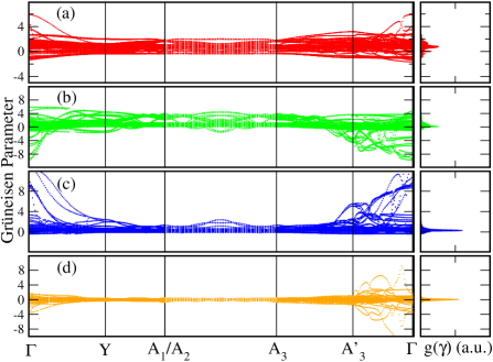
Figure 2: The Grüneisen parameters $\gamma_{i,\lambda{\boldsymbol{q}}}$ of NbS₃-IV along the high-symmetry directions for (a) type $1$ ($x$ uniaxial), (b) type $2$ ($y$ uniaxial), (c) type $3$ ($z$ uniaxial), and (d) type $5$ ($xz$ strain). The selected ${\boldsymbol{q}}$ points are the same as in Fig. 1. The right panels are the corresponding densities of Grüneisen parameters $g_{i}(\gamma)$.

We then evaluate $\Gamma_{i}(\nu)$, the phonon density of states weighted by the Grüneisen parameters, for $i=1,2,3,5$. A $30\times 30\times 10$ mesh is used for the ${\boldsymbol{q}}$-point sampling. Fig. 3(b) shows very high anisotropies of the Grüneisen parameters associated with different deformations. There is a gap between $407$ to $519$ cm^-1 in all $\Gamma_{i}(\nu)$, which is similar to that of the phonon density of states shown in Fig. 1(b). The results show that high-frequency modes (around $550$ cm^-1) are dominated by negative Grüneisen parameters. The dependency of the heat capacity on temperature shown in Fig. 3(a) tells us that these modes contribute to $I_{i}(T)$ (via Eq. 11) only at high temperatures. The deformation due to an $xz$ shear strain gives $\Gamma_{5}(\nu)$ which is only slightly anharmonic relative to that of the diagonal deformations (i.e., $\Gamma_{1}(\nu)$, $\Gamma_{2}(\nu)$, and $\Gamma_{3}(\nu)$). These diagonal deformations are mostly positive, except for $\Gamma_{2}(\nu)$ in the range of $50$ to $75$ cm^-1.

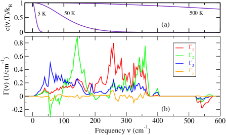
Figure 3: (a) The heat capacity $c(\nu,T)$ as a function of phonon frequency $\nu$ at $5$, $50$, $500$ K. (b) $\Gamma_{i}(\nu)$, the phonon density of states weighted by the Grüneisen parameters as a function of frequency $\nu$ corresponding to type $i$ deformation, for $i=1,2,3,5$.

The integrated quantities $I_{i}(T)$ for $i=1$, $2$, $3$, and $5$ are shown in Fig. 4 may be obtained through either a direct summation in the ${\boldsymbol{q}}$-space according to Eq. 9 or through an integral over the frequencies according to Eq. 11. It is seen that $I_{1}(T)$ is larger than $I_{2}(T)$ and $I_{3}(T)$ at high temperatures above $100$ K, which is consistent with the data in Fig. 3(b). It is seen that $I_{5}(T)$ is indeed small compared to the diagonal quantities $I_{1}(T)$, $I_{2}(T)$, and $I_{3}(T)$ over the entire temperature range, which is again consistent with the small values of $\Gamma_{5}(\nu)$ shown in Fig. 3(b).

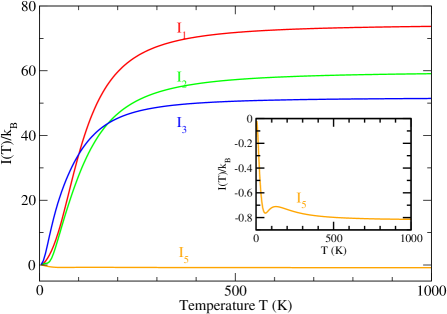
Figure 4: Integrated quantities $I_{i}(T)$ for different deformations. The insert shows the detailed variations of $I_{5}(T)$.

The TEC tensor components $\alpha_{i}$, $i=1,2,3,5$ are displayed as solid lines in Fig. 5. It is somewhat surprising that $\alpha_{1}(T)$ is the smallest among all diagonal TEC tensor components, despite the fact that $I_{1}(T)$ is the dominant diagonal component, at least for $T>100$ K as shown in Fig. 4. We can rationalize this result as follows. According to Eq. 13, $\alpha_{1}(T)$ is a linear combination of $I_{i}(T)$, weighted by coefficients taken from the first row of the elastic compliance matrix $S$ in Eq. 34. Since $S_{13}=-3.20\times 10^{-3}$/GPa is negative and large in magnitude compared to $S_{11}=5.97\times 10^{-3}$/GPa, and $I_{1}(T)$ and $I_{3}(T)$ are comparable in magnitudes, this makes $\alpha_{1}(T)$ the smallest among all diagonal $\alpha_{i}(T)$. It should be noted that $\alpha_{1}(T)$ is negative between $0$ and $50$ K (shown in the inset of Fig. 5) partly because $I_{3}(T)$ is dominant for temperatures below $100$ K. On the other hand, the dominant value of $S_{33}=22.84\times 10^{-3}$/GPa over $S_{31}$ and $S_{32}$ makes $\alpha_{3}(T)$ the dominant diagonal TEC tensor component. Thus, we conclude that the value of a TEC depends on not only on the anharmonic effects measured by the Grüneisen parameters, as commonly believed, but also on the mechanical properties such as the elastic constants (or equivalently, the elastic compliance matrix). The volumetric TEC of NbS₃-IV is $\alpha_{v}=34\times 10^{-6}$ K^-1 at high temperatures.

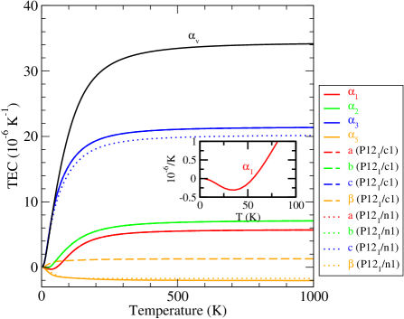
Figure 5: The TEC tensor components $\alpha_{i}$ for $i=1,2,3,5$, the lattice parameter TECs for $P12_{1}/c1$ and $P12_{1}/n1$ settings are shown as functions of temperature. Note that $\alpha_{2}(T)=\alpha_{\beta}(T)=\alpha_{\beta^{\prime}}(T)$. $\alpha_{a}(T)=\alpha_{a^{\prime}}(T)\approx\alpha_{1}(T)$. $\alpha_{c}(T)\approx\alpha_{3}(T)$.

Next, we turn to the discussion of the lattice-parameter TECs for the crystal in a $P12_{1}/c1$ setting with $\beta=89.98^{\circ}$. Firstly, $\alpha_{b}(T)=\alpha_{2}(T)$ by the choice of the unique axis. From Fig. 5, we find that $\alpha_{a}(T)$ is indistinguishable from $\alpha_{1}(T)$ since the primitive lattice vector ${\boldsymbol{a}}$ is parallel to the $x$ axis at $0$ K and it is always almost parallel to the $x$ axis even at higher $T$ due to small values of $\alpha_{5}(T)$. For this setting in which $\beta$ is very close to $90^{\circ}$, the primitive lattice vector ${\boldsymbol{c}}$ remains almost parallel to the $z$-axis at all temperatures, causing $\alpha_{c}(T)$ to be indistinguishable from $\alpha_{3}(T)$. We find that $\alpha_{\beta}(T)$ can be approximated very well (not shown) by $-\frac{2}{\pi}\alpha_{5}(T)$, since $\beta(T)$ is always very close to ${\frac{1}{2}}\pi$ and that $\beta={\frac{1}{2}}\pi-\epsilon_{5}$ (the physical meaning of $\epsilon_{5}$ is the decrease in angle between two elements in the $x$ and $z$ directions, see, e.g., Ref. Nye, 1985), and hence $\alpha_{\beta}=\frac{1}{\beta}{\frac{d\beta}{dT}}=-\frac{1}{\beta}\alpha_{5}(T)\approx-\frac{2}{\pi}\alpha_{5}(T)$.

We discuss next the lattice-parameter TECs of a new primitive cell derived from the $P12_{1}/c1$ setting with $\beta=89.98^{\circ}$, using the transformation rule as shown in Eq. 5. It turns out that this corresponds to a $P12_{1}/n1$ settingNespolo and Aroyo (2016) with $\beta^{\prime}=110.50^{\circ}$, $a^{\prime}=a=6.673$, $b^{\prime}=b=4.870$, $c^{\prime}=19.042$ Å. Since this setting also describes the same unrotated crystal as the $P12_{1}/c1$ setting, the TEC tensor components remain the same. For this new $P12_{1}/n1$ setting, we evolve the monoclinic lattice parameters as previously performed for the $P12_{1}/c1$ setting. It is not surprising to find that $\alpha_{b^{\prime}}(T)=\alpha_{b}(T)=\alpha_{2}(T)$. In addition, $\alpha_{a^{\prime}}(T)=\alpha_{a}(T)$, both of which are essentially the same as $\alpha_{1}(T)$. However, we do find that $\alpha_{c^{\prime}}(T)$ is somewhat different from $\alpha_{3}(T)$ as a result of the primitive lattice vector ${\boldsymbol{c}}^{\prime}$ being oriented away from $z$ axis. Finally, $\alpha_{\beta^{\prime}}(T)$ has an opposite sign compared to $\alpha_{\beta}(T)$ and agrees fortuitously with $\alpha_{5}(T)$.

IV Summary

With an extension of the Grüneisen formalism, we have, for the first time, studied the thermal expansion properties of a monoclinic phase of niobium trisulfide (NbS₃) using density-functional theory calculations. Large anisotropies in the thermal expansion coefficient (TEC) tensor components in the $x$, $y$, $z$ directions have been found. A negative TEC tensor component $\alpha_{11}$ is found at low temperatures, the occurence of which is mainly due to the mechanical property characterized by the elastic compliance. This is somewhat surprising since a negative TEC is usually associated with the occurence of many phonon modes with negative Grüneisen parameters. We expect that the Grüneisen parameters generated in this work could be used to provide a good estimate of the thermal conductivity based on a Slack’s expressionToher et al. (2014); Slack (1979); Blanco et al. (2004). The obtained Grüneisen parameters can be further used to extract third-order interatomic force constants for the determination of thermal conductivity by solving the Boltzmann transport equationLi et al. (2014); Lindsay (2016). Our developed method can be applied to any crystal classes, which opens the door to studying many important materials at the level of accurate density-functional theory.

V Acknowledgments

We thank the National Supercomputing Center, Singapore (NSCC) and A*STAR Computational Resource Center, Singapore (ACRC) for computing resources. This work is supported in part by RIE2020 Advanced Manufacturing and Engineering (AME) Programmatic Grant No A1898b0043.

Appendix A Obtaining the TEC tensor from the lattice-parameter TECs

Given the lattice-parameter TECs $\alpha_{a}(T)$ $\alpha_{b}(T)$, $\alpha_{c}(T)$, and $\alpha_{\beta}(T)$, and temperature dependence of the primitive lattice vectors ${\boldsymbol{a}}$, ${\boldsymbol{b}}$, and ${\boldsymbol{c}}$ where ${\boldsymbol{a}}(T)=a_{1}(T){\boldsymbol{i}}+a_{3}(T){\boldsymbol{k}}$, ${\boldsymbol{b}}(T)=b_{2}(T){\boldsymbol{j}}$, and ${\boldsymbol{c}}=c_{1}(T){\boldsymbol{i}}+c_{3}(T){\boldsymbol{k}}$, we seek to obtain the TEC tensor components $\alpha_{i}(T)$, for $i=1,2,3,5$. As mentioned before, we have immediately $\alpha_{2}(T)=\alpha_{b}(T)$. In the following we present a method to calculate $\alpha_{i}(T)$ for $i=1,3,5$.

Consider $a(T)=\sqrt{a_{1}(T)^{2}+a_{3}(T)^{2}}$, we have

$$a^{\prime}=\frac{a_{1}a_{1}^{\prime}+a_{3}a_{3}^{\prime}}{a}$$ (35)

where $y^{\prime}$ means the derivative of $y$ with respect to $T$. We have suppressed the explicit dependence of all quantities on temperature in Eq. 35 for clarity. Replacing $a_{1}^{\prime}$ and $a_{3}^{\prime}$ using Eqs. 29 and 30 we have

$$a_{1}^{2}\alpha_{1}+a_{3}^{2}\alpha_{3}+a_{1}a_{3}\alpha_{5}=a^{2}\alpha_{a}$$ (36)

The three unknowns $\alpha_{1}$, $\alpha_{3}$, and $\alpha_{5}$ are seen to appear in a linear equation. Therefore we need two other linear equations to enable a matrix inversion. A second relation is obtained by considering $c(T)=\sqrt{c_{1}(T)^{2}+c_{3}(T)^{2}}$ that gives

$$c_{1}^{2}\alpha_{1}+c_{3}^{2}\alpha_{3}+c_{1}c_{3}\alpha_{5}=c^{2}\alpha_{c}$$ (37)

The third relation is obtained by differentiating ${\boldsymbol{a}}\cdot{\boldsymbol{c}}=a_{1}c_{1}+a_{3}c_{3}=ac\cos\beta$ with respect to $T$. Collecting all three relations, we have

$$\begin{pmatrix}a_{1}^{2}&a_{3}^{2}&a_{1}a_{3}\\ c_{1}^{2}&c_{3}^{2}&c_{1}c_{3}\\ 2a_{1}c_{1}&2a_{3}c_{3}&a_{1}c_{3}+a_{3}c_{1}\end{pmatrix}\begin{pmatrix}\alpha_{1}\\ \alpha_{3}\\ \alpha_{5}\end{pmatrix}=R$$ (38)

where

$$R^{T}=[a^{2}\alpha_{a},c^{2}\alpha_{c},ac(\alpha_{a}+\alpha_{c})\cos\beta-ac\beta\alpha_{\beta}\sin\beta]$$ (39)

An inversion of Eq. 38 leads to

$$\begin{pmatrix}\alpha_{1}\\ \alpha_{3}\\ \alpha_{5}\end{pmatrix}=\frac{1}{(ac\sin\beta)^{2}}\begin{pmatrix}c_{3}^{2}&a_{3}^{2}&-a_{3}c_{3}\\ -2c_{1}c_{3}&-2a_{1}a_{3}&a_{1}c_{3}+a_{3}c_{1}\\ c_{1}^{2}&a_{1}^{2}&-a_{1}c_{1}\end{pmatrix}R$$ (40)

Recall all quantities on the right hand side of Eq. 40 depend on $T$, we then have explicit (albeit complicated) expressions for $\alpha_{1}(T)$, $\alpha_{3}(T)$, and $\alpha_{5}(T)$. It may be pointed out that these expressions for TEC tensor components are somewhat different from that found in Ref. 31, presumably due to the fact that they always orient the $c$ lattice parameter so that it is pointing in the $z$ Cartesian direction. Specifically they have $\alpha_{2}(T)=\alpha_{b}(T)$ and $\alpha_{3}(T)=\alpha_{c}(T)$. However, we do not impose such condition but to allow the crystal to freely change its shape under the effect of temperature while keeping the Cartesian coordinates fixed.

References

- Goodwin et al. [2008] A. L. Goodwin, M. Calleja, M. J. Conterio, M. T. Dove, J. S. O. Evans, D. A. Keen, L. Peters, and M. G. Tucker, Science 319, 794 (2008).
- Lin et al. [2011] J. Lin, L. Guo, Q. Huang, Y. Jia, K. Li, X. Lai, and X. Chen, Phys. Rev. B 83, 125430 (2011).
- Kim et al. [2012] Y. Kim, X. Chen, J. Shi, I. Miotkowski, Y. P. Chen, P. A. Sharma, A. L. L. Sharma, M. A. Hekmaty, Z. Jiang, and D. Smirnov, Appl. Phys. Lett. 100, 071907 (2012).
- Mounet and Marzari [2005] N. Mounet and N. Marzari, Phys. Rev. B 71, 205214 (2005).
- Stoffel et al. [2015] R. P. Stoffel, V. L. Deringer, R. E. Simon, R. P. Hermann, and R. Dronskowski, J. Phys.: Condens. Matter 27, 085402 (2015).
- Calabrese et al. [1991] J. Calabrese, N. L. Jones, R. L. Harlow, N. Herron, D. L. Thorn, and Y. Wang, J. Am. Chem. Soc. 91, 2328 (1991).
- Du et al. [2017] K.-Z. Du, Q. Tu, X. Zhang, Q. Han, J. Liu, S. Zauscher, and D. B. Mitzi, Inorg. Chem. 56, 9291 (2017).
- Giovanni et al. [2018] D. Giovanni, W. K. Chong, Y. Y. F. Liu, H. A. Dewi, T. Yin, Y. Lekina, Z. X. Shen, N. Mathews, C. K. Gan, and T. C. Sum, Adv. Sci. 5, 1800664 (2018).
- Zhao and Vanderbilt [2002] X. Zhao and D. Vanderbilt, Phys. Rev. B 65, 075195 (2002).
- Haggerty et al. [2014] R. P. Haggerty, P. Sarin, Z. D. Apostolov, P. E. Driemeyer, and W. M. Kriven, Journal of the American Ceramic Society 97, 2213 (2014).
- Ding and Xiao [2015] Y. Ding and B. Xiao, RSC Adv. 5, 18391 (2015).
- Liu et al. [2017] G. Liu, H. M. Liu, J. Zhou, and X. G. Wan, J. Appl. Phys. 121, 045104 (2017).
- Gan and Lee [2018] C. K. Gan and C. H. Lee, Comput. Mater. Sci. 151, 49 (2018).
- Grüneisen [1926] E. Grüneisen, Handb. Phys. 10, 1 (1926).
- Schelling and Keblinski [2003] P. K. Schelling and P. Keblinski, Phys. Rev. B 68, 035425 (2003).
- Monserrat et al. [2013] B. Monserrat, N. D. Drummond, and R. J. Needs, Phys. Rev. B 87, 144302 (2013).
- Huang et al. [2016] L.-F. Huang, X.-Z. Lu, E. Tennessen, and J. M. Rondinelli, Comput. Mater. Sci. 120, 84 (2016).
- Barron and Klein [1974] T. H. K. Barron and M. L. Klein, in Dynamical Properties of Solids, edited by G. K. Horton and A. A. Maradudin (North-Holland, Amsterdam, 1974) p. 391.
- Shiomi et al. [2011] J. Shiomi, K. Esfarjani, and G. Chen, Phys. Rev. B 84, 104302 (2011).
- Lee and Gan [2017] C. H. Lee and C. K. Gan, Phys. Rev. B 96, 035105 (2017).
- Bloodgood et al. [2018] M. A. Bloodgood, P. Wei, E. Aytan, K. N. Bozhilov, A. A. Balandin, and T. T. Salguero, APL Materials 6, 026602 (2018).
- Ribeiro et al. [2018] G. A. S. Ribeiro, L. Paulatto, R. Bianco, I. Errea, F. Mauri, and M. Calandra, Phys. Rev. B 97, 014306 (2018).
- Zhao et al. [2011] Y. Y. Zhao, K. T. E. Chua, C. K. Gan, J. Zhang, B. Peng, Z. P. Peng, and Q. H. Xiong, Phys. Rev. B 84, 205330 (2011).
- Chong et al. [2014] W. K. Chong, G. Xing, Y. Liu, E. L. Gui, Q. Zhang, Q. Xiong, N. Mathews, C. K. Gan, and T. C. Sum, Phys. Rev. B 90, 035208 (2014).
- van Smaalen [1988] S. van Smaalen, Phys. Rev. B 38, 9594 (1988).
- Jellinek [1960] F. Jellinek, Nature 185, 376 (1960).
- Rijnsdorp and Jellinek [1978] J. Rijnsdorp and F. Jellinek, J. Solid State Chem. 25, 325 (1978).
- Zettl et al. [1982] A. Zettl, C. Jackson, A. Janossy, G. Grüner, A. Jacobsen, and A. Thompson, Solid State Commun. 43, 345 (1982).
- Zybtsev et al. [2017] S. G. Zybtsev, V. Y. Pokrovskii, V. F. Nasretdinova, S. V. Zaitsev-Zotov, V. V. Pavlovskiy, A. B. Odobesco, W. W. Pai, M.-W. Chu, Y. G. Lin, E. Zupanič, H. J. P. van Midden, S. Šturm, E. Tchernychova, A. Prodan, J. C. Bennett, I. R. Mukhamedshin, O. V. Chernysheva, A. P. Menushenkov, V. B. Loginov, B. A. Loginov, A. N. Titov, and M. Abdel-Hafiez, Phys. Rev. B 95, 035110 (2017).
- Hahn [Ed.] T. Hahn(Ed.), International Tables for Crystallography (2006). Vol. A, Space-group symmetry (Chester, International Union of Crystallography, 2006).
- Schlenker et al. [1975] J. L. Schlenker, G. V. Gibbs, and M. B. Boisen, Jr., American Mineralogist 60, 828 (1975).
- Nye [1985] J. F. Nye, Physical Properties of Crystals: Their Representations by Tensors and Matrices (Clarendon, Oxford, 1985).
- Baroni et al. [2001] S. Baroni, S. de Gironcoli, A. Dal Corso, and P. Giannozzi, Rev. Mod. Phys. 73, 515 (2001).
- Kresse et al. [1995] G. Kresse, J. Furthmüller, and J. Hafner, Europhys. Lett. 32, 729 (1995).
- Ackland et al. [1997] G. J. Ackland, M. C. Warren, and S. J. Clark, J. Phys.: Condens. Matter 9, 7861 (1997).
- Alfè [2009] D. Alfè, Comp. Phys. Comm. 180, 2622 (2009).
- Gan et al. [2015] C. K. Gan, J. R. Soh, and Y. Liu, Phys. Rev. B 92, 235202 (2015).
- Beckstein et al. [2001] O. Beckstein, J. E. Klepeis, G. L. W. Hart, and O. Pankratov, Phys. Rev. B 63, 134112 (2001).
- Dal Corso [2016] A. Dal Corso, J. Phys.: Condens. Matter 28, 075401 (2016).
- Gan and Liu [2016] C. K. Gan and Y. Y. F. Liu, Phys. Rev. B 94, 134303 (2016).
- Kresse and Furthmüller [1996] G. Kresse and J. Furthmüller, Comput. Mater. Sci. 6, 15 (1996).
- Gan et al. [2010] C. K. Gan, X. F. Fan, and J.-L. Kuo, Comput. Mater. Sci. 49, S29 (2010).
- Liu et al. [2014] Y. Liu, K. T. E. Chua, T. C. Sum, and C. K. Gan, Phys. Chem. Chem. Phys. 16, 345 (2014).
- Nespolo and Aroyo [2016] M. Nespolo and M. I. Aroyo, Acta Cryst. A 72, 523 (2016).
- Toher et al. [2014] C. Toher, J. J. Plata, O. Levy, M. de Jong, M. Asta, M. BuongiornoNardelli, and S. Curtarolo, Phys. Rev. B 90, 174107 (2014).
- Slack [1979] G. A. Slack, in Solid State Physics, edited by H. Ehrenreich, F. Seitz, and D. Turnbull (Academic, New York, 1979) p. 1.
- Blanco et al. [2004] M. A. Blanco, E. Francisco, and V. Luaña, Comp. Phys. Comm. 158, 57 (2004).
- Li et al. [2014] W. Li, J. Carrete, N. A. Katcho, and N. Mingo, Comp. Phys. Comm. 185, 1747 (2014).
- Lindsay [2016] L. Lindsay, Nano. Micro. Thermo. Eng. 20, 67 (2016).