Statistical signature of vortex filaments in classic turbulence: dog or tail?

Abstract

The title of this paper echoes the title of a paragraph in the famous book by Frisch on classical turbulence. In the relevant chapter, the author discusses the role of the statistical dynamics of vortex filaments in the fascinating problem of turbulence and the possibility of a breakthrough in constructing an advanced theory. This aspect arose due to the large amount of evidence, both experimental and numerical, that the vorticity field in turbulent flows has a pronounced filamentary structure. In fact, there is unquestionably a strong relationship between the dynamics of chaotic vortex filaments and turbulent phenomena. However, the question arises as to whether the basic properties of turbulence (cascade, scaling laws. etc.) are a consequence of the dynamics of the vortex filaments (the ‘dog’ concept), or whether the latter have only a marginal significance (the ‘tail’ concept). Based on well-established results regarding the dynamics of quantized vortex filaments in superfluids, we illustrate how these dynamics can lead to the main elements of the theory of turbulence. We cover key topics such as the exchange of energy between different scales, the possible origin of Kolmogorov-type spectra and the free decay behavior.

I Introduction

I.1 Quantum turbulence vs classical turbulence

The idea that classical turbulence (CT) can be modeled by the dynamics of a set of slim vortex tubes (or vortex sheets) has been discussed for quite a long time (a good exposition of the prehistory of that question can be found in the famous books by Frisch Frisch (1995), and by Chorin Chorin (1994) ). The main motivation for this idea is related to incredible complexity in the traditional formulation of this tantalizing problem. Indeed, as Migdal Migdal (1986) wrote: ”Hydrodynamics over the centuries has been described by partial differential equations. This description turned out to be adequate for laminar flows, but faced difficulties in the phenomena of turbulence. The source of these difficulties is the choice of velocity field components $\mathbf{v(r},t)$ as dynamic variables. This field behaves stochastically in turbulent flows, which makes the differential equations useless. The required number of degrees of freedom exceeds the capabilities of any computer. The vortex filaments can be considered as elementary excitations of the turbulent flow. Their dynamics, although unusual, is actually more simple than the dynamics of waves and particles, and requires less computer resources”.

Beside this motivation regarding new breakthrough methods in the theory of CT, there are also numerous observations that the vorticity field in turbulent flows has a pronounced filamentary structure. The range of evidences extends from 500-year-old drawings of eddy motion made by Leonardo da Vinci (see e.g., Frisch (1995) or Tsubota and Kobayashi (2009)) up to modern powerful numerical simulations (see, e.g. Vincent and Meneguzzi (1991)). In fact, there is unquestionably a relationship between the dynamics of a chaotic vortex filament and turbulent phenomena. However, the question arises as to whether the properties of turbulence are a consequence of the dynamics of the vortex filaments, or whether the latter have only a marginal significance. To highlight this issue, Frisch Frisch (1995) entitled a chapter in his book devoted to this topic as ”Statistical signature of vortex filaments: Dog or tail?”

In classical fluids, the concept of thin vortex tubes is rather the fruitful mathematical model. Quantum fluids, where vortex filaments are real objects, provide an excellent opportunity for studying the question of whether the chaotic dynamics of a set of quantized vortex lines (quantum turbulence or QT) can reproduce the properties of real hydrodynamic turbulence. This feature of QT is usually referred as the quasi-classical regime.

In principle, there is large huge amount of scientific researches on quantum turbulence and its relation to classic turbulence (CT) in conventional fluids, the according material is summarized in series of recent review articles Vinen (2000), Kobayashi and Tsubota (2005),Vinen (2010),Skrbek and Sreenivasan (2012),Tsubota et al. (2013),Barenghi et al. (2014),Walmsley et al. (2007). However, the vast majority of research in this area uses the ideas and results of CT to explain phenomena in QT, i.e. CT $\rightarrow$ QT. It can be said that the relationship between QT and CT is such that the former is a recipient and the latter is a donor. In the current article the, opposite direction is chosen, it is we who are trying to state what properties of QT phenomena can be used to explain some features of CT, i.e. QT $\rightarrow$ CT. This statement corresponds to the question submitted in the manuscript title – DOG OR TAIL.

I.2 What this article is and is not about

The main goal of this paper is to discuss which elements of the quantized vortex dynamics, established and studied recently, would lead to the main ingredients of theory of classic turbulence. Before proceeding with the content of the work, it seems useful to make some appropriate reservations, based on preliminary discussions.

First of all this work does not claim that the chaotic dynamics of discrete (quantized) vortex filaments can simulate classical turbulence. Indeed, as it was written above this idea had been discussed by other scientists, who observed, or supposed, or obtained from numerical experiments, that the vorticity field has a filamentary structure. I pursue a more modest goal, which is simply to disclose the “dog’s concept” on the basis of well-known facts from the researches of discrete quantum vortices in superfluids. And this is not a review article, rather it is application of the well established results on dynamics of quantized vortices to concrete physical problem.

Secondly, in order to clarify the question formulated by Frisch Frisch (1995) concerning only vortex filaments, I did not consider the possible role of other vortex structures, such as vortex sheets or vortex bundles.

Furthermore, in order to concentrate on the main goal (without distracting the readers from the basic ideas), I avoid a detailed description of complicated mathematical calculations. Instead, I refer to the original papers in which the detailed technique is presented.

In addition, since our primary purpose was to understand the essence of turbulent phenomena in terms of vortex filaments, I confined myself to analytical studies that have quantitative conclusions. Indeed, although numerical modeling also leads to results that are relevant to the quasiclassical QT regime (for example, the Kolmogorov spectra), the origin of these phenomena is hidden behind a numerical procedure.

Finally, I also confine myself to the most pronounced features of the turbulent flow, such as the exchange of energy between different scales (Sec. II), Kolmogorov’s energy spectra (Section III), and the free decay of QT (Section IV).

II Exchange of energy between different scales.

II.1 Kinetics of vortex loops

The first topic that we will discuss concerns a basic feature of turbulent flows, i.e. the exchange of energy between different scales. In the case of QT this effect is quite expected, since the dynamics of quantized vortex filaments is essentially nonlinear. However, the concrete implementation of this phenomenon in terms of lines is not clear. In this Section, we will consider one of the possible mechanisms that leads to the energy cascade, this is the kinetics of colliding vortex loop, constituting the QT.

This model assumes that the vortex tangle consists of a set of many closed vortex loops, which undergo an enormous number of reconnections and self-reconnections, involving (for typical experiments) several millions of collisions per second (per cm³). Thus, in the full statement of the problem, we are dealing with a set of objects (vortex loops) which do not have a fixed number of elements and which can be born and die. Additionally the objects (vortex loops) themselves possess an infinite number of degrees of freedom with very involved dynamics. Clearly, this problem can hardly be resolved in the near future, and substantial simplifications are required. One of the possible treatments of this problem is to impose a condition whereby the vortex loops have a pre-defined structure, namely the random walking structure. The idea that one-dimensional topological defects have a random walking structure is widely used (see, e.g., books by Kleinert Kleinert (1990)). For vortex loops in superfluid helium this idea is realized in form of the so-called generalized Wiener distribution, which takes into account the anisotropy, polarization and finite curvature Nemirovskii (1998).

It is assumed here that the “own” dynamics of the vortex loop are omitted; to some extent, this is absorbed by the random walk model and the parameters of the generalized Wiener distribution. We can then consider the evolution of the vortex tangle as the free motion of vortex loops that have a predetermined random walk structure. All interactions are reduced to collisions (self-collisions) and recombinations of loops, as shown in Fig. 1. This approach allows for a detailed investigation of the kinetics of vortex tangle, corresponding studies have been performed in Nemirovskii (2006, 2008, 2013a).

To demonstrate the existence of energy cascade in space of scales, the usual variant of the Wiener distribution had been chosen with an elementary step $\xi_{0}$ of the order of the intervortex distance $\xi_{0}\sim\delta=$ $\mathcal{L}^{-1/2}$, where $\mathcal{L}$ is the vortex line density (VLD).

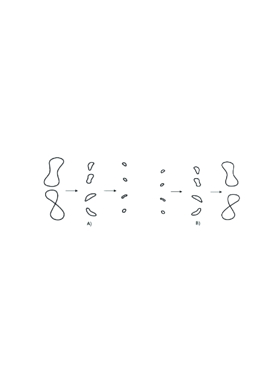
Figure 1: The cascade -like breaking down and merging of Gaussian vortex loops due to reconnection and self-reconnection processes.

Then, the only degree of freedom which exists is the length $l$ of the loop, and it is natural to introduce the distribution function of of time dependent number density of loops $n(l,t)$ (per unit volume) with length$\ l$. The temporal evolution of the quantity $n(l,t)$ can be studied on the basis of the Boltzmann-type “balance equation”, which is a highly nonlinear integral equation. Using a special and elegant technique developed by Zakharov (see, e.g. Zakharov et al. (1992)), it was demonstrated that the stationary balance equation has an exact power-like solution for the distribution function $n(l)$, namely $n(l)=const\ast l^{-5/2}$ Nemirovskii (2006, 2008, 2013a). This is not equilibrium solution; it describes the flux of the length of loops in space of their sizes. The term ”flux”  here means just the redistribution of length among the loops due to reconnections. The stated approach generates a number of predictions that can be associated with the quasiclassical behavior of quantum turbulence.

The main prediction related to the topic of this paper concerns the constant flux of energy in the space of scales. The solution described above corresponds to a non-equilibrium state, and describes a flux $P^{L}(l)$ of length density $L(l,t)=ln(l,t)$, which represents length accumulated in loops of size $l$ in $l-$space. Furthermore we assume that due to the extremely small core radius of the vortex filament the length of vortex line does not change during reconnection event. Conservation of the vortex line density can be expressed in the form of a continuity equation for the length density $L(l,t)$

$$\frac{\partial L(l,t)}{\partial t}+\frac{\partial P^{L}(l)}{\partial l}=0.$$ (1)

In the stationary case, the expression for the $l$-independent flux $P^{L}$ can be directly derived from the balance equation, again with the use of the Zakharov technique Zakharov et al. (1992). The according calculations were performed in the papers cited above Nemirovskii (2006, 2008, 2013a) and suggest the following result for the flux of energy $P^{E}$

$$P^{E}=C_{F}\kappa(\kappa\mathcal{L})^{2}.$$ (2)

Constant $C_{F}$ was named in honor of Richard Feynman, who was the first to discuss the decay of superfluid turbulence due to the cascade-like breaking down of vortex loops Feynman (1955). We changed the $l$ independent flux $P^{L}$  of the length of loops by the energy flux $P^{E}$, since in the local induction approximation (LIA) the energy $E$ of a line (up to factor $\rho_{s}\kappa$, where $\rho_{s}$ is the superfluid density and $\kappa$ is quantum of circulation of vortex filament) is equal to its length $L$. Therefore Eq. (1) describes the constant flux of the vortex energy $P^{E}(l)=const$ in the space of scales (which is here just the space loop sizes $l$).

The flux $P^{E}$ consists of two contributions: the first, positive one is related to the merging of loops, and is responsible for delivering the energy to large scales, while the second, negative contribution appears to be due to the breaking-down of loops (see Fig. 1), and describes a flux of energy to small scales. Depending on the temperature, either one can prevail; this depends just on the temperature behavior of structure constants of the vortex tangle. In particular, at very low temperature $C_{F}\ \approx-0.25$ (see Nemirovskii (2006, 2008, 2013a)), the energy flux is negative, i.e. $P^{E}<0$, and the energy is transferred into the region of small scales. This corresponds to the direct cascade in classical turbulence.

A relation of type (2) is also known as a Vinen equation. It describes attenuation of the vortex line density after switching off the counterflow of He II. It was obtained in a purely phenomenological way using experimental data. For low temperatures, $C_{F}\$ is of the order of $0.1$, which agrees by the order of the quantity with our estimation.

Each vortex loop induces a three-dimensional velocity field. The whole ensemble of loops generates a random velocity field that can be considered turbulent motion. It is clear that large vortex loops create a three-dimensional velocity field that can be associated with large-scale motion. Thus, it can be argued that the process of the cascade-like breaking down of vortex loops can be associated with the main feature of turbulence – the constant Kolmogorov-Richardson flux of energy in the space of scales with the consequent dissipation of kinetic energy at very small scales. As Feynman wrote ”a vortex ring can break up into smaller and smaller rings. The eventual small rings may be identical to rotons. Then all the energy of the vortex will eventually end by forming large numbers of rotons, that is, heat” (see Feynman (1955), citation is slightly adapted)

II.2   Stochastic deformation of loops

Another mechanism for the exchange of energy between scales, inherent for turbulent phenomena, is related to the nonlinear dynamics of a single vortex filament (neglecting the reconnections). We can describe the solution to the problem of nonlinear chaotic distortions of a vortex loop Nemirovskii and Baltsevich (2001) as follows. The chaotic motion of a quantized vortex filament obeys a Langevin type equation

$${\frac{{\partial~{}}\mathbf{s}{(\xi,t)}}{{\partial~{}t}}}~{}={\frac{\kappa}{{4\pi}}}\int{\frac{[\mathbf{s}(\xi^{\prime},t)-\mathbf{s}(\xi,t)]\times\mathbf{s}_{\xi^{\prime}}^{\prime}}{{|\mathbf{s}(\xi^{\prime},t)-\mathbf{s}(\xi,t)|^{3}}}}d\xi^{\prime}+\mathbf{\eta}(\xi,t)+\mathbf{\zeta}(\xi,t).$$ (3)

Here $\mathbf{s}{(\xi,t)}$ is the position vector of the line points labelled by the arc length ${\xi}$, which varies in the interval $0<\xi<l,\ \$. The quantity $\mathbf{\eta}(\xi,t)$ stands for dissipation, which acts for marginally small scales; and the quantity $\mathbf{s}^{\prime}{(\xi,t)}$ is the tangent vector. The stirring Langevin force $\mathbf{\zeta}(\xi,t)$ is assumed to be Gaussian with a space correlator concentrated at large scales (of order of the loop size $l$). Explicit forms of both $\eta(\xi,t)$ and $\zeta(\xi,t)$ are not essential, since their action is realized at the extreme ends of the interval, namely at very small and large scales, respectively. In the intermediate region, the so called the inertial interval, the influence of both $\eta(\xi,t)$ and $\zeta(\xi,t)$ is imperceptible and everything is determined by the Biot-Savart law, as expressed by the first term on the right-hand side of Eq. (3). This term controls nonlinear processes and determines spectral characteristics and flux of energy The role of the Langevin force $\zeta(\xi,t)$ and dissipation $\eta(\xi,t)$  is reduced to the creation of additional length (energy) in the large scale region and dissipation of this excessive length in very small scales. That implies that the length generated by random force is transferred along the spectrum to be dissipated at small scales.

An example of the evolution of an initially smooth vortex ring, which obeys the equation (3), obtained in direct numerical simulation (see Nemirovskii et al. (1991)), is depicted in Fig. 2.

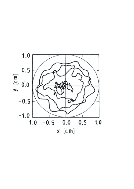
Figure 2: Evolution of a vortex ring under the influence of an external random force in the local approach (Eq. 3); as predicted, a consequent emergence of higher harmonics takes place leading eventually to an entanglement of the initially smooth vortex loop.

An analytical study was performed in Nemirovskii and Baltsevich (2001)  on the basis of the so-called local induction approximation (LIA), which allows us to reformulate the Biot-Savart integral in Eq. (3) in a local nonlinear form. The reduced LIA problem in Eq. (3) can be formulated in the $p$ space, where $p$ is the one-dimensional wave vector, conjugated to the variable $\xi$. In this form it has an analytical solution Nemirovskii and Baltsevich (2001), based on a theoretical trick known as the direct interaction approximation (DIA) for diagramming technique, elaborated for classical turbulence by Wyld Wyld (1961).

One of the results arising from this solution concerns the energy conservation in the $p$ space, which obviously coincides with the space of scales (and which to some extent is equivalent the three-dimensional space of scales)

$${\frac{{\partial E_{p}}}{{\partial t}}}~{}+~{}{\frac{{\partial}P_{p}^{E}}{{\partial p}}}~{}=I_{+}(p)~{}-~{}I_{-}(p).$$ (4)

Here $E_{p}={\frac{1}{\sqrt{2\pi}}}\int_{0}^{l}\mathbf{s}_{p}^{\prime}\mathbf{s}_{-p}^{\prime}e^{-ip\xi}d\xi$ is the one dimensional energy spectrum in the LIA (up to factor $\rho_{s}\kappa^{2}$), and $P_{p}^{E}$ is the flux of energy in Fourier space. The right-hand side of Eq. (4) describes the creation of additional length (energy) at a rate of $I_{+}^{K}(p)$ due to the stirring force and its annihilation due to the dissipative mechanism (at a rate of $-I_{-}^{K}(p)$). In a region of wave numbers $p$, remote from both the scale of pumping $p_{+}$ and the sink $p_{-},\;\;p_{+}~{}\ll~{}p~{}\ll~{}p_{-}$ , the so called inertial interval, the derivative (in stationary situation) $\partial P_{p}^{E}/\partial p=0$ , so $P_{p}^{E}$ is constant. It has therefore been shown that the evolution of a quantized vortex filament due to its “own” nonlinear dynamics results in a constant flux of energy in the space of harmonics  $p$.

As in the previous subsection we assume that small $p$ harmonics, corresponding to large scales (in space of the label variable $\xi$) induce a velocity field associated with large scale motion in real three-dimensional space. Accordingly, large $p$ harmonics generate a small scale three-dimensional motion. Therefore the nonlinear exchange of energy between different harmonics can be associated with the Kolmogorv-Richardson flux of energy in a real turbulent flow.

Based on the results presented in this section, it can be argued that the chaotic dynamics of vortex filaments indeed results in a constant flux of energy of three-dimensional flow, which is the main feature of turbulence. Thus, in the question “dog or tail?”, these examples weigh in favor of the “dog”.

III Kolmogorov-type spectra generated by vortex filaments

Probably, the strongest argument in favour of the quasi-classical behavior of QT is the $k$ dependence ($k=\left|\mathbf{k}\right|$, $\mathbf{k}$ is the wave number) of the energy spectra$\ E(k)$ of the three-dimensional velocity field, induced by quantized vortices. Many numerical simulations, which have been performed both for vortex filament method for superfluid helium (see, e.g. Araki et al. (2002),Kivotides et al. (2002); Kivotides et al. (2001a), Procaccia and Sreenivasan (2008)) and with the use of the Gross-Pitaevskii equation for Bose-Einstein condensate (Nore et al. (1997a, b), Kobayashi and Tsubota (2005),Tsubota and Kobayashi (2009); Sasa et al. (2011), Nemirovskii (2014)), have demonstrated a Kolmogorov-type dependence $E(k)\varpropto\,k^{-5/3}$. The origin of this phenomenon in terms of vortex line dynamics is unclear, details are hidden behind a numerical procedure.

We now discuss how the dynamics of vortex filaments can result in a Kolmogorov type spectrum. The energy $E$ of the vortex line configuration $\{\mathbf{s}(\xi)\}$ is an integral over the wave vectors $\mathbf{k}$ (see Nemirovskii et al. (2002)),

$$E(\mathbf{k)}=\frac{{\rho}_{s}{\kappa}^{2}}{2(2\pi)^{3}}\int\limits_{\mathbf{k}}\frac{d^{3}\mathbf{k}}{\mathbf{k}^{2}}\int\limits_{0}^{L}\int\limits_{0}^{L}\mathbf{s}^{\prime}(\xi_{1})\cdot\mathbf{s}^{\prime}(\xi_{2})d\xi_{1}d\xi_{2}\exp\left[i\int\limits_{\xi_{1}}^{\xi_{2}}\mathbf{k\cdot s}^{\prime}(\tilde{\xi})d\tilde{\xi}\right].$$ (5)

Note that the energy spectrum $E\left(\mathbf{k}\right)$ can be easily derived from the expression for the Fourier transform of the velocity field $v_{\mathbf{k}}=$ $\mathbf{k}\times\mathbf{\omega}_{\mathbf{k}}/k^{2}$. Taking into account that $\mathbf{k\cdot\omega}_{\mathbf{k}}=0$, and that the vorticity field $\mathbf{\omega(r)}$ can be written as

$$\mathbf{\omega}(\mathbf{r})=\nabla\times\mathbf{v}_{s}=\kappa\int\mathbf{s}^{\prime}(\xi)\;\delta(\mathbf{r}-\mathbf{s}(\xi,t))d\xi,$$ (6)

one easily obtains equation (5). In the isotropic case, the spectral density depends on the absolute value of the wave number $k$. Integrating over solid angle leads to formula (see Kondaurova and Nemirovskii (2005)):

$$E(k)=\frac{\rho_{s}\kappa^{2}}{(2\pi)^{2}}\int\limits_{0}^{L}\int\limits_{0}^{L}\mathbf{s}^{\prime}(\xi_{1})\cdot\mathbf{s}^{\prime}(\xi_{2})\frac{\sin(k\left|\mathbf{s}(\xi_{1})-\mathbf{s}(\xi_{2})\right|)}{k\left|\mathbf{s}(\xi_{1})-\mathbf{s}(\xi_{2})\right|}d\xi_{1}d\xi_{2}.$$ (7)

Equations (5)-(5) are key relations, which relate the vortex line configuration $\{\mathbf{s}(\xi)\}$ with the spectrum of energy. On this ground there was investigated a number of various configurations of a set of vortex filament appeared on superfluid flows (see brief review Nemirovskii (2013b)). These results were obtained using a straight line and vortex ring. We also studied uniform and non-uniform vortex arrays, a fractal vortex filament, a straight line with excited Kelvin waves on it, and the case of reconnecting vortex filaments. Among of the listed above cases there is two configurations $\{\mathbf{s}(\xi)\}$,which indeed lead to the Kolmogorov spectrum. These are the reconnecting vortex filaments  and Kelvin waves on straight (smooth) line. Let’s follow how they generate the spectrum $E(k)\varpropto\,k^{-5/3}$ and give some comments

III.1 Reconnecting Vortex Filaments

During evolution of the quantum turbulence, vortex filaments undergo an enormous number of collisions and reconnection events. The dynamics of the line in the process of reconnection possesses many features that have a universal character (see e.g. de Waele and Aarts (1994)). This occurs as a collapse of the approaching vortex filaments, concentrating large amounts of energy at the points of connection of the line. The idea that collapsing singular solutions can play a significant role in formation of turbulent spectra is currently being intensively discussed (see e.g. Kuznetsov and Ruban (2000), Kerr (2013)). The classical examples of this type of spectra are the Phillips spectrum for water-wind waves, created by white caps/wedges on the surface of water, and the Kadomtsev-Petviashvili spectrum for acoustic turbulence, created by shock waves. An attractive direction for research is to elaborate this idea for the case of reconnection of vortex filaments in superfluids. In our view, the situation discussed below is a further example confirming the value of this idea.

Over a series of publications (see e.g. Siggia (1985),de Waele and Aarts (1994), Kerr (2013),Boué et al. (2013),Andryushchenko et al. (2017)), it has been shown that very near to the point of collision, the vortex filaments have a universal form (see. Fig. 3, left). An analytical expression for the shape of the curves was proposed in Boué et al. (2013). This expression for the two lines $\{s(\xi_{1})\},\{s(\xi_{2})\}$ was used by the author Nemirovskii (2014) to calculate an energy spectrum $E(k)$ on the basis of (angle averaged) Eq. (5). An investigation was carried out using a method of asymptotic expansion of integrals containing rapidly oscillating functions, which arise in equations (5)-(5) (see e.g. Fedoryuk (1977)).

From Fig. 3 (Right) it can be seen that for reconnecting lines the spectrum is close to $E(k)\propto k^{-5/3}$. The interval of wave numbers in which the spectrum $E(k)$ $\approx k^{-5/3}$ (straight line) is observed is regulated by the curvature of the kink and the intervortex space $\delta$, which is chosen to be equal to unity. In reality this spectrum covers a maximum of about $\ 1.5$ decades around $k\approx$ $2\pi/\delta$. It should be stressed, however, that in the key numerical works (see the references above), the ranges for wave number are also of the order of one decade around $k\approx$ $2\pi/\delta$.

In a real vortex tangle, where the number of reconnection is large, the quantity $\delta$ can vary for different events, This can lead to an effective enlarging of the interval over which the Kolmogorov spectrum is realized.

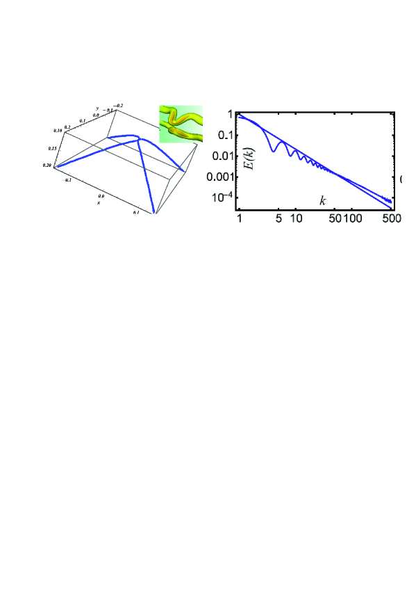
Figure 3: (Color online) Left. Touching quasi-hyperbolae describing collapsing lines Boué et al. (2013). The inset shows, as an example, the kinks on the anti-parallel collapsing vortex tubes obtained from numerical simulation Bustamante and Kerr (2008). The figure from numerics of Bustamante and Kerr is taken to illustrate that the both classical and quantum vortices implement reconnection in very similar manner. Right. The energy spectrum $E(k)$ of the three-dimensional velocity field, induced by this configuration.

III.2 1D Kelvin waves spectrum and 3D velocity spectrum

In the literature there is discussed the idea of obtaining the 3D velocity spectrum just by putting it equal to the energy spectrum $E_{KW}(k)$ of 1D Kelvin waves. For instance, as stated in Kivotides et al. (2001b):”We notice that, because the fluctuations of the velocity field are induced by the Kelvin wave fluctuations on the filaments, it is reasonable  to expect that

$$E(k)\sim E_{KW}(k).$$ (8)

The same conjecture was used in papers by L’vov et al.(see e.g., L’vov et al. (2008)). Details of this activity can be read in a series of papers by L’vov, Nazarenko and coauthors L’vov et al. (2007).L’vov et al. (2008); Sasa et al. (2011); Boué et al. (2011)

Consider the exact solution to this problem on the basis of the general Eqs. (5)-(7). A straight line (along the $z$ axis) with running Kelvin waves on it can be represented in terms of a vector $s(\xi,t)$ in the following form: $s(\xi,t)=(x(z,t),y(z,t),z)$. We introduce the two-dimensional vector $a\rho(z,t)=(x(z,t),y(z,t))$, where the amplitude $a$ is assumed to be much smaller than the wave length $\lambda$. Substituting it into (7) and expanding in powers of $a$, we get,

$$E(k) = \frac{{\rho}_{s}{\kappa}^{2}}{4\pi^{2}}\int\limits_{0}^{L}\int\limits_{0}^{L}dz_{1}dz_{2}{\LARGE\{}\frac{\sin\left(k\left|z_{2}-z_{1}\right|\right)}{k\left|z_{2}-z_{1}\right|}+\frac{a^{2}\cos\left(k\left|z_{2}-z_{1}\right|\right)(\mathbf{\rho}(z_{2})-\mathbf{\rho}(z_{1}))^{2}}{2\left|z_{2}-z_{1}\right|^{2}}$$ (9)

$$-\frac{a^{2}\sin\left(k\left|z_{2}-z_{1}\right|\right)(\mathbf{\rho}(z_{2})-\mathbf{\rho}(z_{1}))^{2}}{2k\left|z_{2}-z_{1}\right|^{3}}+\frac{a^{2}(\mathbf{\rho}^{\prime}(z_{1})\cdot\mathbf{\rho}^{\prime}(z_{2})\sin\left(k\left|z_{2}-z_{1}\right|\right)}{k\left|z_{2}-z_{1}\right|}{\LARGE\}}$$

The first term of the zero-order in amplitude $a$ exactly coincides with the energy spectrum induced by the unperturbed straight line, as it should be. Correspondingly it gives $E_{straight}(k)\sim\rho_{s}\kappa^{2}/k$.

To move further we have to find the correlation characteristics for the fluctuating vector of displacement $\rho(z_{2})$. The main contribution in the theory of stochastic nonlinear Kelvin waves and their role in superfluid turbulence was made in a series of works by Svistunov Svistunov (1995), Kozik & Svistunov Kozik and Svistunov (2004, 2005, 2009, 2010) and in papers by L’vov & Nazarenko with coauthors L’vov et al. (2008); Laurie et al. (2010); Boué et al. (2011); Lebedev and L’vov (2010). Following these works we accept that the Kelvin waves ensemble has the following power-like spectrum:

$$\left\langle\mathbf{\rho}(p)\cdot\mathbf{\rho}(-p)\right\rangle=Ap^{-s}.$$ (10)

We take here the notation $p$ for the one-dimensional vector, conjugated to $z$, reserving the notation $k$ for the absolute value of the wave vector of the 3D field. The formula (10) implies that (see, e.g., Frisch (1995), Eqs. (4.60),(4.61)) the squared increment for the vector of displacement scales as, $\left\langle(\mathbf{\rho}(z_{2})-\mathbf{\rho}(z_{1}))^{2}\right\rangle\varpropto(z_{2}-z_{1})^{s-1}$. Then the second order correlator $\left\langle(\mathbf{\rho}^{\prime}(z_{2})\mathbf{\rho}^{\prime}(z_{1}))\right\rangle$ scales as $\left\langle(\mathbf{\rho}^{\prime}(z_{2})\mathbf{\rho}^{\prime}(z_{1}))\right\rangle\varpropto(z_{2}-z_{1})^{s-3}$. Substituting it into (10) and counting the powers of quantity $k$, we conclude that the correction $E_{KW}(k)$ to the spectrum $E(k)$, due to the ensemble of Kelvin waves has a form:

$$E_{KW}(k)\varpropto{a}^{2}k^{-s+2}.$$ (11)

It is remarkable fact that this quantity coincides formally with the one-dimensional spectrum of KW $\delta E(p)\varpropto a^{2}p^{-s+2}$. In series papers L’vov, Nazarenko and coauthors L’vov et al. (2008); Sasa et al. (2011); L’vov et al. (2007); Boué et al. (2011)it was proposed the spectrum for Kelvin waves of shape (10) with $s=11/3$, therefore the 3D spectrum of velocity field $\delta E(k)\varpropto k^{-5/3}$, i.e. the Kolmogorov type energy spectrum.

Thus, the 3D motion of superfluid helium induced by chaotic nonlinear Kelvin waves, indeed possesses the Kolmogorov type spectrum. The contribution $E_{KW}(k)$ is small in comparison with the energy accumulated in the term $E_{straight}(k)$, by virtue of the smallness of the wave amplitudes $a$, and disappears with the KW. There is a view, however, that just like in the 2D case, when the ”own” energy of point vortices, no matter how huge, does not affect the collective dynamics of the vortex ensemble Nazarenko (2013).

In this section, it was demonstrated that the dynamics of the lines generate the vortex

filament configurations $\{\mathbf{s}(\xi)\}$, which induce a three-dimensional velocity field with a

Kolmogorov-type spectrum. Thus, again, in the question of whether the vortices are the “dog” or the “tail”, these examples weigh in favor of the “dog”.

IV Free decay of quantum turbulence.

In this section, we consider another line of evidence regarding the quasi-classical character of quantum turbulence, which relates to the free decay of QT. This subject is of particular interest, since it has been properly studied using experimental measurements. Arguments have been put forward that if quantum turbulence behaves in a similar way to classic turbulence, then the long-term dependence of the VLD $\mathcal{L}(t)$ is the power-like function $t^{-3/2}$ Skrbek and Sreenivasan (2012),Vinen (2010),Bradley et al. (2006),Walmsley et al. (2007). The basis for this result was the belief that at large scales, the flow of the superfluid component obeys the laws of classical turbulence. This results in the obsevation that the dissipation rate $\varepsilon$ (coinciding with flux of energy $P^{E}$, see Eq. (2) ) scales as $t^{-3}$, $\varepsilon\propto t^{-3}$. Combining this result with Eq. (2), we arrive at $L(t)\propto t^{-3/2}$.

There is a number of experimental works in which this dependence is indeed observed. One convincing result of an experiment of this type, performed by the Manchester group Walmsley et al. (2007) is depicted in the upper right-hand section of Fig 4. It can clearly be seen that the long-term dependence is indeed $\mathcal{L}(t)\propto t^{-3/2}$.

Again, despite the exposed above ideas on the origin of the dependence $\mathcal{L}(t)\propto t^{-3/2}$, it is not clear how this arises directly from the dynamics of vortex lines.

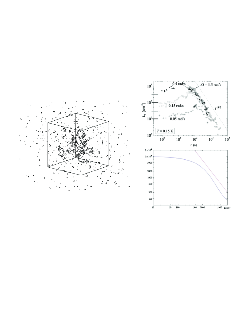
Figure 4: Left: The emission of small loops from the bulk; results of direct numerical simulation (see, Kondaurova and Nemirovskii (2012)). Right: Comparison with experiment; the upper section shows the temporal attenuation of the vortex line density, obtained from experiment Walmsley et al. (2007). The temporal behavior of the same quantity calculated on the basis of the diffusion mechanism in (Eq.12) Nemirovskii (2010).

We now discuss the mechanism of free decay of quantum turbulence which is based on the dynamics of vortex filaments and which predicts the dependence $\mathcal{L}(t)\propto t^{-3/2}$. This mechanism is related to the emission of small loops from the bulk. As discussed earlier, a large number of very small loops appear during the reconnection cascade. However, due to their small size, these loops have high mobility and escape from the volume. An example of this behavior, obtained by direct numerical simulation (see, Kondaurova and Nemirovskii (2012)), is shown in the left-hand section of Fig. 4. This process occurs in a diffusion-like manner.

The quantitative theory of the diffusion-like spreading of the VT, with the consequent decay of quantum turbulence, was developed by the author, and details can be found in Nemirovskii (2010). The vortex loops composing the vortex tangle can move as a whole, with a drift velocity $V_{l}$ depending on their structure and their length. The loops moving in space carry the length of the line, the energy, the momentum, and so on. In the case of an inhomogeneous vortex tangle, the net flux $\mathbf{J}$ of the vortex length appears due to the gradient of concentration of the vortex line density $\mathcal{L}(x,t)$. The situation here is exactly the same as in classical kinetic theory, with the difference being that the “carriers” are not point particles but extended objects (vortex loops), which themselves possess an infinite number of degrees of freedom with very involved dynamics. It is possible to carry out an investigation based on the supposition that vortex loops have a Brownian or random walk structure with a generalized Wiener distribution. To develop a theory of transport processes fulfilled by vortex loops (in the spirit of classical kinetic theory), we need to calculate the drift velocity $V_{l}$ and the free path $\lambda(l)$ for a loop of size $l$. The free path $\lambda(l)$ is very small, implying that only very small loops make a significant contribution to transport processes, e.g. a loop of size equal to the interline space $\delta=\mathcal{L}^{-1/2}$ can fly (on average) about $2-3$ times the distance $\delta$. However, when the vortex tangle becomes sufficiently dilute, the larger loops can move a distance comparable with the size of the bulk. Referring to Nemirovskii (2010) we write down here the final result. The flux $\mathbf{J}$ of vortex lines is proportional to $\nabla\mathcal{L}$; $\mathbf{J}=D_{v}\nabla\mathcal{L}$; and, correspondingly, the spatial-temporal evolution of quantity $\mathcal{L}$ obeys the diffusion-type equation

$$\frac{\partial\mathcal{L}}{\partial t}=D_{v}\nabla^{2}\mathcal{L}.$$ (12)

Here the diffusion constant $D_{v}\approx 2\kappa$. To clarify whether this mechanism is able to sustain the decay of the QT observed in the Manchester experiments Walmsley et al. (2007), we calculated the evolution of the VLD $\mathcal{L}(t)$ solving the diffusion equation, for the cases corresponding to these experimental conditions. The results are shown in the lower right-hand section of Fig. 4. It is evident that this theoretical result based on the diffusion model, is in very good agreement with the experimental data.

Thus, based on a theoretical analysis of the vortex line dynamics, we have demonstrated how processes occurring in the ensemble of vortex loops lead to the behavior observed in classical turbulence that again supports the “dog” concept.

V Conclusion and Discussion

We therefore demonstrate that certain results obtained for quantum fluids, which have been considered to be arguments in favor of the idea of modeling classical turbulence using a set of chaotic quantized vortices, can be explained using the frame of theoretical models dealing with the dynamics of vortex filaments.

Of course, one can object that the current arguments are not strong enough to claim that the issue has been definitively settled, and that the phenomena described above have nothing to do with the real turbulence. Nevertheless, taking into account the tantalizing problem of classical turbulence, the hope of solving it using a new breakthrough approach seems very attractive. Thus, the following bifurcation arise. An optimistic view is that these approaches do indeed relate to the real turbulence, and that we have new insight into processes occurring in turbulent flow. A pessimistic view is that the phenomena described above have nothing to do with the real turbulence, and that this effect is a coincidence. However, we hope in any event that this paper will have a stimulating effect on related activity.

The study of Sections II-A, III, IV was carried out under state contract with IT SB RAS (АААА-А17-117022850027-5), the study of subsections II-B III-B was financially supported by RFBR / Russian Science Foundation (Project No. 18-08-00576).

References

- Frisch (1995) U. Frisch, Turbulence (Cambridge University Press, Cambridge, 1995).
- Chorin (1994) A. Chorin, Vorticity and turbulence, Applied mathematical sciences (Springer-Verlag, 1994).
- Migdal (1986) A. Migdal, Voprosi Kibernetiki p. 122 (1986).
- Tsubota and Kobayashi (2009) M. Tsubota and M. Kobayashi, in Progress in Low TEMPERATURE PHYSICS: QUANTUM TURBULENCE, edited by M. Tsubota and W. Halperin (Elsevier, 2009), vol. 16 of Progress in Low Temperature Physics, pp. 1 – 43.
- Vincent and Meneguzzi (1991) A. Vincent and M. Meneguzzi, Journal of Fluid Mechanics 225, 1 (1991).
- Vinen (2000) W. F. Vinen, Phys. Rev. B 61, 1410 (2000).
- Kobayashi and Tsubota (2005) M. Kobayashi and M. Tsubota, Phys. Rev. Lett. 94, 065302 (2005).
- Vinen (2010) W. Vinen, Journal of Low Temperature Physics 161, 419 (2010).
- Skrbek and Sreenivasan (2012) L. Skrbek and K. R. Sreenivasan, Physics of Fluids 24, 011301 (pages 48) (2012).
- Tsubota et al. (2013) M. Tsubota, M. Kobayashi, and H. Takeuchi, Physics Reports 522, 191 (2013), ISSN 0370-1573, quantum hydrodynamics.
- Barenghi et al. (2014) C. F. Barenghi, L. Skrbek, and K. R. Sreenivasan, Proceedings of the National Academy of Sciences 111, 4647 (2014).
- Walmsley et al. (2007) P. M. Walmsley, A. I. Golov, H. E. Hall, A. A. Levchenko, and W. F. Vinen, Phys. Rev. Lett. 99, 265302 (2007).
- Kleinert (1990) H. Kleinert, Gauge Fields in Condenced Matter Physics (World Scientific, Singapore, 1990).
- Nemirovskii (1998) S. K. Nemirovskii, Phys. Rev. B 57, 5972 (1998).
- Nemirovskii (2006) S. K. Nemirovskii, Phys. Rev. Lett. 96, 015301 (2006).
- Nemirovskii (2008) S. K. Nemirovskii, Phys. Rev. B 77, 214509 (2008).
- Nemirovskii (2013a) S. K. Nemirovskii, Physics Reports 524, 85 (2013a).
- Zakharov et al. (1992) V. E. Zakharov, V. S. L’vov, and G. Falkovich, Kolmogorov Spectra of Turbulence I (Springer-Verlag, Berlin, 1992).
- Feynman (1955) R. P. Feynman, Progress in Low Temperature Physics, Vol. 1 (North-Holland, Amsterdam, 1955), p. 17.
- Nemirovskii and Baltsevich (2001) S. Nemirovskii and A. Baltsevich, in Quantized Vortex Dynamics and Superfluid Turbulence, edited by C. Barenghi, R. Donnelly, and W. Vinen (Springer Berlin Heidelberg, 2001), vol. 571 of Lecture Notes in Physics, pp. 219–225, ISBN 978-3-540-42226-6.
- Nemirovskii et al. (1991) S. K. Nemirovskii, J. Pakleza, and W. Poppe, Notes et Documents LIMSI (Laboratoire d’Informatique pour la Mecanique et les Sciences de l’Ingenieur) No. 91-14, 1991).
- Wyld (1961) H. W. Wyld, Annals of Physics 14, 143 (1961).
- Araki et al. (2002) T. Araki, M. Tsubota, and S. K. Nemirovskii, Phys. Rev. Lett. 89, 145301 (2002).
- Kivotides et al. (2002) D. Kivotides, C. J. Vassilicos, D. C. Samuels, and C. F. Barenghi, EPL (Europhysics Letters) 57, 845 (2002).
- Kivotides et al. (2001a) D. Kivotides, C. F. Barenghi, and D. C. Samuels, Europhys. Lett. 54, 771 (2001a).
- Procaccia and Sreenivasan (2008) I. Procaccia and K. Sreenivasan, Physica D: Nonlinear Phenomena 237, 2167 (2008), euler Equations: 250 Years On - Proceedings of an international conference.
- Nore et al. (1997a) C. Nore, M. Abid, and M. E. Brachet, Phys. Rev. Lett. 78, 3896 (1997a).
- Nore et al. (1997b) C. Nore, M. Abid, and M. E. Brachet, Physics of Fluids 9, 2644 (1997b).
- Sasa et al. (2011) N. Sasa, T. Kano, M. Machida, V. S. L’vov, O. Rudenko, and M. Tsubota, Phys. Rev. B 84, 054525 (2011).
- Nemirovskii (2014) S. K. Nemirovskii, Physical Review B 90, 104506 (2014).
- Nemirovskii et al. (2002) S. K. Nemirovskii, M. Tsubota, and T. Araki, Journal of Low Temperature Physics 126, 1535 (2002).
- Kondaurova and Nemirovskii (2005) L. Kondaurova and S. K. Nemirovskii, Journal of Low Temperature Physics 138, 555 (2005).
- Nemirovskii (2013b) S. Nemirovskii, Journal of Low Temperature Physics 171, 504 (2013b).
- de Waele and Aarts (1994) A. T. A. M. de Waele and R. G. K. M. Aarts, Phys. Rev. Lett. 72, 482 (1994).
- Kuznetsov and Ruban (2000) E. Kuznetsov and V. Ruban, Journal of Experimental and Theoretical Physics 91, 775 (2000).
- Kerr (2013) R. M. Kerr, Physics of Fluids 25, 065101 (2013).
- Siggia (1985) E. D. Siggia, Phys. Fluids 28, 794 (1985).
- Boué et al. (2013) L. Boué, D. Khomenko, V. S. L’vov, and I. Procaccia, Phys. Rev. Lett. 111, 145302 (2013).
- Andryushchenko et al. (2017) V. A. Andryushchenko, L. P. Kondaurova, and S. K. Nemirovskii, Journal of Low Temperature Physics 187, 523 (2017), ISSN 1573-7357.
- Fedoryuk (1977) M. V. Fedoryuk, Method of Saddle Points. (Nauka, Moscow, 1977).
- Bustamante and Kerr (2008) M. D. Bustamante and R. M. Kerr, Physica D: Nonlinear Phenomena 237, 1912 (2008).
- Kivotides et al. (2001b) D. Kivotides, J. C. Vassilicos, D. C. Samuels, and C. F. Barenghi, Phys. Rev. Lett. 86, 3080 (2001b).
- L’vov et al. (2008) V. L’vov, S. Nazarenko, and O. Rudenko, J. Low Temp. Phys. 153, 140 (2008).
- L’vov et al. (2007) V. S. L’vov, S. V. Nazarenko, and O. Rudenko, Phys. Rev. B 76, 024520 (2007).
- Boué et al. (2011) L. Boué, R. Dasgupta, J. Laurie, V. L’vov, S. Nazarenko, and I. Procaccia, Phys. Rev. B 84, 064516 (2011).
- Svistunov (1995) B. V. Svistunov, Phys. Rev. B 52, 3647 (1995).
- Kozik and Svistunov (2004) E. Kozik and B. Svistunov, Phys. Rev. Lett. 92, 035301 (2004).
- Kozik and Svistunov (2005) E. Kozik and B. Svistunov, Phys. Rev. Lett. 94, 025301 (2005).
- Kozik and Svistunov (2009) E. Kozik and B. Svistunov, Journal of Low Temperature Physics 156, 215 (2009).
- Kozik and Svistunov (2010) E. Kozik and B. Svistunov, Phys. Rev. B 82, 140510 (2010).
- Laurie et al. (2010) J. Laurie, V. S. L’vov, S. Nazarenko, and O. Rudenko, Phys. Rev. B 81, 104526 (2010).
- Lebedev and L’vov (2010) V. Lebedev and V. L’vov, Journal of Low Temperature Physics 161, 548 (2010).
- Nazarenko (2013) S. Nazarenko (2013), Private communication.
- Bradley et al. (2006) D. I. Bradley, D. O. Clubb, S. N. Fisher, A. M. Guénault, R. P. Haley, C. J. Matthews, G. R. Pickett, V. Tsepelin, and K. Zaki, Phys. Rev. Lett. 96, 035301 (2006).
- Kondaurova and Nemirovskii (2012) L. Kondaurova and S. K. Nemirovskii, Phys. Rev. B 86, 134506 (2012).
- Nemirovskii (2010) S. K. Nemirovskii, Phys. Rev. B 81, 064512 (2010).