A partition of unity approach to fluid mechanics and fluid-structure interaction

Abstract

For problems involving large deformations of thin structures, simulating fluid-structure interaction (FSI) remains challenging largely due to the need to balance computational feasibility, efficiency, and solution accuracy. Overlapping domain techniques have been introduced as a way to combine the fluid-solid mesh conformity, seen in moving-mesh methods, without the need for mesh smoothing or re-meshing, which is a core characteristic of fixed mesh approaches. In this work, we introduce a novel overlapping domain method based on a partition of unity approach. Unified function spaces are defined as a weighted sum of fields given on two overlapping meshes. The method is shown to achieve optimal convergence rates and to be stable for steady-state Stokes, Navier-Stokes, and ALE Navier-Stokes problems. Finally, we present results for FSI in the case of a 2D mock aortic valve simulation. These initial results point to the potential applicability of the method to a wide range of FSI applications, enabling boundary layer refinement and large deformations without the need for re-meshing or user-defined stabilization.

1 Introduction

Fluid-structure interaction (FSI) problems involving thin solids which undergo large deformations and translations can be encountered in a significant number of engineering applications. In industry, we have examples such as the design of parachutes [1, 2, 3] and wind-turbines [4, 5]. In cardiovascular research, the simulation of valves [6, 7] and implanted devices [8] holds a great potential for better understanding and treatment of a number of pathologies such as valve stenosis, regurgitation, heart failure and outflow obstruction. Building such models, however, remains challenging due to the need to balance computational costs and solution accuracy. In the case of cardiac valves, for example, studies typically require simplifications of the domain’s geometry [9] or the fluid models [10].

FSI approaches for this class of problems can be grouped into three main categories: interface-tracking, interface-capturing and overlapping domains methods [11, 12]. In the case of interface-tracking, the fluid problem is typically based on the Arbitrary Lagrangian-Eulerian (ALE) [13, 14, 15] formulation. This allows for the fluid domain to deform with the solid and enables adjusting the element resolution close to surfaces in order to more accurately represent boundary layers. In [16], an ALE based method is shown to produce superior results when considering moderate deformations to three variations of fictitious domain (examples of interface-capturing) for similar mesh resolutions. However, for large deformations, it is known that the distortion of the fluid mesh can diminish the quality of elements and negatively impact the accuracy of solutions [11]. While multiple re-meshing techniques [17] have been proposed, the process introduces grid interpolation errors and its computational cost effectiveness is linked to the frequency at which the mesh needs to be adjusted. As shown in [18], where the particular case of cardiac valves is discussed, the ALE based simulations take more time to run than competing interface-capturing methods.

In contrast, interface-capturing methods do not require boundary fitted meshes for the fluid and solid and thus avoid the need for re-meshing. Examples include the Fictitious Domain Method [19, 20] (FDM), where the coupling between the solid and fluid is achieved via additional Lagrange multiplier terms [21], and the Immersed Finite Element method (IFEM) [22, 23, 24, 25], where the kinematic constraints between the fluid and solid is imposed through interpolation and distribution of local body forces. While both FDM and IFEM require the construction of a solid mesh, in the Immersed Structural Potential Method (ISPM) [26] both problems are solved on the same mesh, with the solid being represented as a moving collection of quadrature points. However, these methods lack a conforming interface between the fluid and solid and can result in poor approximations of pressure jumps and surface stresses [27, 28]. For this reason, mesh-adaptation [29] and XFEM enrichment [30, 31, 32, 33, 34, 35, 36, 37] techniques have been proposed in order to overcome these issues. Also a significant challenge for interface-capturing, as noted in [38], remains the fact the resolution of the fluid flow around the structural surface is limited by the local element size of the fluid mesh. In practice, this leads to over-refinement of the fluid mesh along the moving trajectory of the solid and to significant increases of the computational costs.

Overlapping domain techniques [39, 40, 41, 42, 43, 44, 45, 46, 12, 47] have been proposed with the aim of combining the advantages of interface-tracking and interface capturing techniques: fluid-solid mesh conformity, boundary layer tracking and eliminating re-meshing. The crux of these methods is the decomposition of the fluid problem into a background coarse component and solution-enriching embedded component that envelops the structures. A challenging aspect, however, is the coupling of the two fluid domains which has to be done weakly due the non-matching fluid-fluid interface. The use of Lagrange multipliers for example, see [30], is impeded by the need to properly choose function spaces in order to guarantee that the inf-sup condition holds for arbitrary moving interfaces. Alternatively, stabilization techniques can be employed to circumvent the inf-sup condition [48, 49, 50]. Overlapping mesh methods for the Stokes problem [51, 52, 46] which use Nitsche’s method [53] avoid introducing an additional Lagrange multiplier field, but nevertheless they require additional, parameter-dependent stabilization terms for the velocity and pressure jump in the vicinity of the fluid-fluid interface to guarantee optimal convergence rates and good system conditioning irrespective of the particular overlap configuration.

In this paper, we propose a new flexible and robust overlapping domain method which uses the partition of unity (PUFEM) approach [54, 55] to decompose the fluid domain into a background mesh and an embedded mesh which can overlap in an arbitrary manner. On each mesh, standard mixed and inf-sup stable velocity-pressure function spaces using Taylor-Hood elements are defined. In the final finite element formulation of the fluid problem, a unified global function space is then used which is defined by taking a properly weighted sum of the function spaces associated with each mesh. To avoid ill-conditioning of the resulting system, additional constraints are introduced in (parts of) the overlap region.

The rest of this paper is structured as follows. After briefly recalling the classical mixed finite element approach for the Stokes problem in Section 2.1, we introduce its PUFEM based overlapping domain formulation including a detailed description of the domain set-up, weighted function spaces, and imposed constraints, see Section 2.2, followed by a short discussion of some computational aspects in Section 2.3. Then in Section 3, we explain how to combine the PUFEM approach with an ALE formulation of the Navier-Stokes problem to treat moving fluid domain and fluid–structure interaction problems. In Section 4, a number of numerical experiments are conducted. First, we investigate the stability and accuracy of our PU approach for a number of fluid flow problems posed on fixed static domains, see Section 4.1–4.3. To demonstrate the capability to handle large changes in the fluid domain geometry, we then consider a fluid flow driven by a oscillating cylinder in Section 4.4 before we turn to a full FSI problem in Section 4.5, where we compare a classical ALE-based approach with our novel combined ALE-PUFEM discretization for a two-dimensional mock aortic valve simulation. Finally in Section 5, we summarize our results and discuss potential future developments.

2 A Partition of unity finite element method for the Stokes problem

In this section, we introduce the main concepts and the basic setup for PUFEM. We begin by reviewing the classic mixed FEM approach to Stokes flow (Section 2.1) and present the key differences introduced in the PUFEM approach (Section  2.2). Finally, in Section 2.3, we describe the process by which we identify the polygonal intersections of overlapping elements and perform the necessary integrations.

2.1 Classical mixed FEM approach to Stokes problems

Let $\Omega_{f}\subset\mathbb{R}^{d}$ be an arbitrary fluid domain on which we solve our problem. Since our focus is oriented towards FSI simulations, we also introduce a solid domain $\Omega_{s}$ which for now, we consider to be fixed and rigid. The boundary of the fluid problem, $\Gamma$, is composed of three, non-overlapping regions: the portions where Dirichlet and Neumann boundary conditions are applied, ($\Gamma_{D}$ and $\Gamma_{N}$, respectively), and the fluid-solid interface, $\Gamma_{fs}$. We then can write Stokes problem as: find the $(\textbf{v},p)$ such that,

$$\mu\nabla^{2}\textbf{v}-\nabla p =\mathbf{0} \text{ in }\Omega_{f},$$ (1a)

$$\nabla\cdot\textbf{v} =0 \text{ in }\Omega_{f},$$ (1b)

$$\left(\mu\nabla\textbf{v}-p\textit{{I}}\right)\cdot\textbf{n} =\textbf{t}_{N} \text{ on }\Gamma_{N},$$ (1c)

v $$=\textbf{v}_{D} \text{ on }\Gamma_{D},$$ (1d)

v $$=\mathbf{0} \text{ on }\Gamma_{\mathit{fs}},$$ (1e)

where $\mu$ is the fluid dynamic viscosity constant. For simplicity, we consider that the Neumann boundary condition tractions are null, i.e. $\textbf{t}_{N}=\mathbf{0}$.

In the case of the Stokes problem in (1), the classic continuous weak form can be written as: find $(\textbf{v},p)\in\boldsymbol{\mathcal{V}}_{D}\times\mathcal{W}$ such that,

$$\int_{\Omega}\mu\nabla\textbf{v}:\nabla\textbf{w}-p\nabla\cdot\textbf{w}+q\nabla\cdot\textbf{v}\hskip 2.84526ptd\Omega=0,\hskip 14.22636pt\forall\hskip 2.84526pt(\textbf{w},q)\in\boldsymbol{\mathcal{V}}_{0}\times\mathcal{W},$$ (2)

where $\boldsymbol{\mathcal{V}}_{D}$, $\boldsymbol{\mathcal{V}}_{0}\subset\textit{{H}}^{1}(\Omega_{f})$ and $\mathcal{W}=L^{2}(\Omega_{f})$. Here the subscripts $D$ and $0$ indicate that the $\boldsymbol{\mathcal{V}}_{D}$, $\boldsymbol{\mathcal{V}}_{0}\subset\boldsymbol{\mathcal{V}}$ subspaces are built such that they incorporate the Dirichlet and zero boundary value conditions on $\Gamma_{D}$. Proofs of the well-posedness of this problem can be found in [56] and [57]. In the discrete setting, the resulting weak form is: find $(\textbf{v}^{h},p^{h})\in\boldsymbol{\mathcal{V}}^{h}_{D}\times\mathcal{W}^{h}$ such that,

$$\int_{\Omega^{h}_{f}}\mu\nabla\textbf{v}^{h}:\nabla\textbf{w}^{h}-p^{h}\nabla\cdot\textbf{w}^{h}+q^{h}\nabla\cdot\textbf{v}^{h}\hskip 2.84526ptd\Omega=0,\hskip 14.22636pt\forall\hskip 2.84526pt(\textbf{w}^{h},q^{h})\in\boldsymbol{\mathcal{V}}^{h}_{0}\times\mathcal{W}^{h}.$$ (3)

In this study, we will use the classic approach in (3) to compare with the PUFEM approach. In this case, we use the LBB stable $\mathbb{P}^{2}-\mathbb{P}^{1}$ Taylor-Hood elements [58]. Thus, the discrete test and trial function spaces can be defined as:

$$\boldsymbol{\mathcal{V}}^{h} =\{\textbf{v}^{h}\in\textit{{C}}^{0}(\Omega^{h}_{f})\hskip 2.84526pt|\hskip 2.84526pt\textbf{v}|_{\tau}\in\left[\mathbb{P}^{2}(\tau)\right]^{d}\text{ for }\tau\in\mathcal{T}_{f}\},$$ (4a)

$$\mathcal{W}^{h} =\{p^{h}\in C^{0}(\Omega^{h}_{f})\hskip 2.84526pt|\hskip 2.84526ptp|_{\tau}\in\mathbb{P}^{1}(\tau)\text{ for }\tau\in\mathcal{T}_{f}\}.$$ (4b)

Here $\Omega^{h}_{f}$ is a discrete equivalent of $\Omega_{f}$, defined by a tessellation $\mathcal{T}_{f}$. $h$ denotes the element size defined as the diameter of the circumcircle. In preparation for the PUFEM discussion, we can also define $\Omega^{h}_{s}$ as the discrete solid domain. $\mathbb{P}^{k}$ designates the set of polynomial function of order $k$.

Previous works [56, 57] derive a priori error estimates where:

$$||\textbf{v}-\textbf{v}^{h}||_{1}+||p-p^{h}||_{0} \leq C_{1}\inf_{\textbf{w}^{h}\in\boldsymbol{\mathcal{V}}^{h}}||\textbf{v}-\textbf{w}^{h}||_{1}+C_{2}\inf_{q^{h}\in\mathcal{W}^{h}}||p-q^{h}||_{0},$$ (5)

where $C_{1}$ and $C_{2}$ are positive constants independent of $h$, and $||\cdot||_{0}$ and $||\cdot||_{1}$ denote the $L^{2}$ and $\textit{{H}}^{1}$ norms, respectively. Using $\mathbb{P}^{2}-\mathbb{P}^{1}$ elements, if $(\textbf{v},p)\in\textit{{H}}^{3}(\Omega)\times H^{2}(\Omega)$, then from interpolation theory [56]:

$$||\textbf{v}-\textbf{v}^{h}||_{1}+||p-p^{h}||_{0}\leq Ch^{2}\left(|\textbf{v}|_{3}+|p|_{2}\right).$$ (6)

2.2 PUFEM approach to Stokes problems

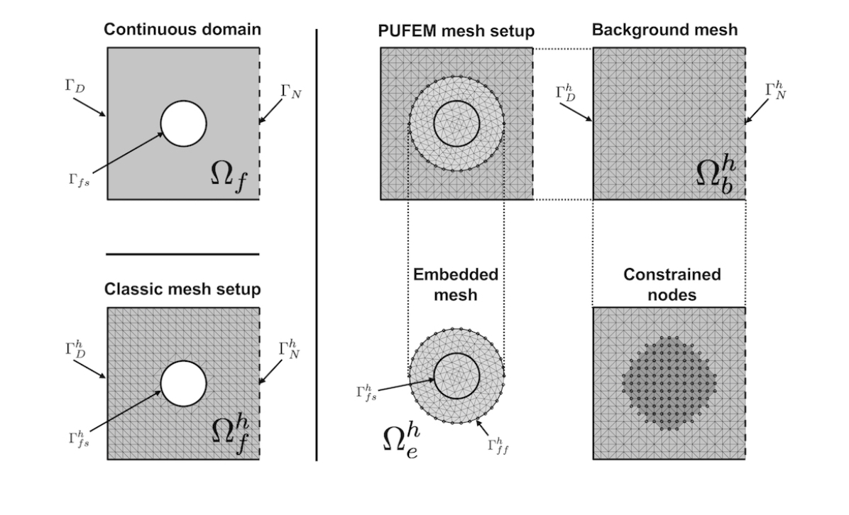
Figure 1: The problem domain in three instances: continuous, classical, single mesh setup and PUFEM setup. In the later, the discrete domain is subdivided into the embedded and background overlapping meshes. Both meshes contain a set of constrained nodes used to avoid ill-conditioning. Here we mark them with circles.

The core difference between the classic approach and the PUFEM setup is that the latter is composed of two overlapping meshes: background and embedded (see Fig. 1), and both have a corresponding discrete domain over which they are defined. Thus, we assume the background domain, $\Omega^{h}_{b}=\Omega^{h}_{f}\cup\Omega^{h}_{s}$, encompasses the entirety of the discrete fluid and solid domains. The embedded domain, $\Omega^{h}_{e}$, which satisfies $\Omega^{h}_{s}\subset\Omega^{h}_{e}\subseteq\Omega^{h}_{b}$, is designed to incorporate the solid and extends into fluid domains providing a boundary layer. The fluid and solid regions of $\Omega^{h}_{e}$ are separated by the $\Gamma^{h}_{\mathit{fs}}$ interface. Additionally, $\Gamma_{\mathit{ff}}^{h}$ is the outer boundary of $\Omega^{h}_{e}$ and serves as its interface with $\Omega^{h}_{b}$. The two meshes each have a corresponding tessellation, $\mathcal{T}_{b}$ and $\mathcal{T}_{e}$, and element sizes denoted by $h_{b}$ and $h_{e}$, respectively. Let $N^{v}_{b}$ and $N^{p}_{b}$ be the set of nodes defining the background mesh in the case of quadratic and linear interpolations. $N^{v}_{e}$ and $N^{p}_{e}$ are their embedded analogues. For the remainder of this paper, we consider the case where the meshes are 2D and triangular.

The discrete weak form for the PUFEM approach can be written as: find $(\textbf{v}^{h},p^{h})\in\textbf{{V}}^{h}_{D}\times W^{h}$ such that,

$$\int_{\Omega^{h}_{b}}\mu\nabla\textbf{v}^{h}:\nabla\textbf{w}^{h}-p^{h}\nabla\cdot\textbf{w}^{h}+q^{h}\nabla\cdot\textbf{v}^{h}\hskip 2.84526ptd\Omega=0,\hskip 14.22636pt\forall\hskip 2.84526pt(\textbf{w}^{h},q^{h})\in\textbf{{V}}^{h}_{0}\times W^{h}$$ (7)

where $\textbf{{V}}^{h}_{D}$, $\textbf{{V}}^{h}_{0}$ and $W^{h}$ are PUFEM function spaces that represent the counterparts of $\boldsymbol{\mathcal{V}}_{D}^{h}$, $\boldsymbol{\mathcal{V}}_{0}^{h}$ and $\mathcal{W}^{h}$ introduced in Section 2.1. The PUFEM function spaces are defined as the weighted sums of function spaces with support on the background and embedded meshes. Thus, based on the same notation of Melenk and Babuska [54], the spaces can be written as:

$$\textbf{{V}}^{h} =\left(1-\psi^{h}\right)\textbf{{V}}^{h}_{{b},*}+\psi^{h}\textbf{{V}}^{h}_{{e},*}$$ (8a)

$$W^{h} =\left(1-\psi^{h}\right)W^{h}_{{b},*}+\psi^{h}W^{h}_{{e},*}$$ (8b)

where the local spaces are defined as:

$$\textbf{{V}}^{h}_{{k},*} =\{\textbf{v}_{k}^{h}\in\textbf{{V}}^{h}_{k}\hskip 2.84526pt|\hskip 2.84526pt\textbf{v}_{k}|_{\textbf{x}}=\textbf{v}_{m}|_{\textbf{x}}\text{ for }\textbf{x}\in\textbf{{X}}^{v}_{k}\}$$ (9a)

$$W^{h}_{k,*} =\{p_{k}^{h}\in W^{h}_{k}\hskip 2.84526pt|\hskip 2.84526ptp_{k}|_{\textbf{x}}=p_{m}|_{\textbf{x}}\text{ for }\textbf{x}\in\textbf{{X}}^{p}_{k}\}$$ (9b)

for $k,m\in\{b,e\}$, $k\neq m$, and

$$\textbf{{V}}^{h}_{{k}} =\{\textbf{v}^{h}\in\textit{{C}}^{0}(\Omega^{h}_{k})\hskip 2.84526pt|\hskip 2.84526pt\textbf{v}^{h}|_{\tau}\in\left[\mathbb{P}^{2}(\tau)\right]^{d}\hskip 2.84526pt\forall\tau\in\mathcal{T}_{k}\}\text{ for }k\in\{b,e\}$$ (10a)

$$W^{h}_{b} =\{p^{h}\in C^{0}(\Omega^{h}_{g})\hskip 2.84526pt|\hskip 2.84526ptp^{h}|_{\tau}\in\mathbb{P}^{1}(\tau)\hskip 2.84526pt\forall\tau\in\mathcal{T}_{b}\}$$ (10b)

$$W^{h}_{e} =\{p^{h}\in L^{2}(\Omega^{h}_{e})\cap\left[C^{0}(\Omega^{h}_{s})\oplus C^{0}(\Omega^{h}_{e}\cap\Omega^{h}_{f})\right]\hskip 2.84526pt|\hskip 2.84526ptp^{h}|_{\tau}\in\mathbb{P}^{1}(\tau)\hskip 2.84526pt\forall\tau\in\mathcal{T}_{e}\}$$ (10c)

Note that with the exception of $W^{h}_{e}$, all the discrete local spaces are continuous.

We allow the functions in $W^{h}_{e}$ to be discontinuous across $\Gamma^{h}_{\mathit{fs}}$ in order to be able to represent the pressure jump between the fluid and embedded solid. The $\textbf{{X}}^{v}_{k}$ and $\textbf{{X}}^{p}_{k}$ sets contain nodes that are constrained in order to avoid ill-conditioning. More details on how these sets are constructed can be found in Section 2.2.1.

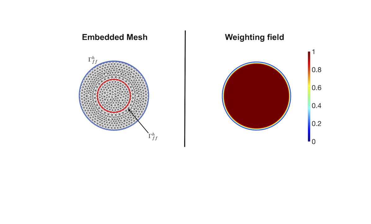
Figure 2: (Left) An example of the embedded mesh with marked fluid-fluid and fluid-solid interfaces. (Right) The resulting weighting field ($\psi^{h}$)

We define the field $\psi^{h}\in V^{h}_{e}$ ($V^{h}_{e}$ is the scalar equivalent of $\textbf{{V}}^{h}_{e}$) such that $\operatorname{supp}(\psi^{h})\subset\Omega^{h}_{e}$, its codomain is $[0,1]$ and $\psi^{h}=0$ on $\Gamma_{\mathit{ff}}^{h}$. For notational simplicity, we consider that all fields defined on the embedded mesh (i.e. $\psi^{h}$, $\textbf{v}^{h}_{e}$ and $p^{h}_{e}$) are zero outside the region of overlap. In practice, we built $\psi^{h}$ using the following series of steps. First, we solved a diffusion problem on the embedded mesh, where we constrain the field to be zero on $\Gamma_{\mathit{ff}}^{h}$ and ten on $\Gamma_{\mathit{fs}}^{h}$. Subsequently, we apply a upper boundary threshold such that the maximum node value is one. Finally, we smoothen the field using the hermitian polynomial $f(u)=-2u^{3}+3u^{2}$. An example of the resulting field in the case of circular mesh can be seen Fig. 2. This approach was used irrespective of element size for consistency. Note however, that this process was chosen on an ad hoc basis. A full investigation on the effects of the support area and shape of $\psi$ remain to be investigated.

One of the benefits that we derive from the weighted form of the PUFEM is that it guarantees a smooth transition across $\Gamma_{\mathit{ff}}^{h}$, irrespective of the mesh size used in either background or embedded mesh. As a result, this should always prevent having mismatched fluxes (i.e. when computed on both sides of the boundary) and the loss of mass across the interface.

2.2.1 Potential sources of ill-conditioning and constraints

Previously we introduced four sets of nodes that we want to constrain $\textbf{{X}}^{v}_{b}$, $\textbf{{X}}^{v}_{e}$, $\textbf{{X}}^{p}_{b}$ and $\textbf{{X}}^{p}_{e}$ and in this subsection we will discuss both their necessity and how we decide which nodes belong to them. With the introduction of the weighting field, the standard basis function support concept becomes insufficient to understand the contribution of each DOF to the total solution. Thus, we introduce a new metric of effective support fraction which for an embedded DOF we define as:

$$E(\textbf{x}_{i})=\left[\int_{\Omega_{f}^{h}}(\psi^{h}\hat{\phi}^{i})^{2}d\Omega\right]\left[\int_{\Omega_{f}^{h}}(\hat{\phi}^{i})^{2}d\Omega\right]^{-1}$$ (11)

where $\hat{\phi}^{i}$ is the basis function of a degree of freedom corresponding to the $\textbf{x}_{i}$ node coordinate. Note that in the case of a background DOF we replace $\psi^{h}$ with $1-\psi^{h}$. As $E(\textbf{x}_{i})\rightarrow 0$ due to a particular overlap configuration, the contribution of DOFs corresponding to $\textbf{x}_{i}$ become very small. If $E=0$ then the contribution to the PUFEM solution is null and the system matrix becomes singular. Thus, we define the four sets of constrained nodes as follows:

$$\textbf{{X}}^{v}_{e} =\{\textbf{x}_{i}\in N^{v}_{e}\hskip 2.84526pt|\hskip 2.84526pt\textbf{x}_{i}\in\Gamma^{h}_{\mathit{ff}}\},$$ (12a)

$$\textbf{{X}}^{p}_{e} =\{\textbf{x}_{i}\in N^{p}_{e}\hskip 2.84526pt|\hskip 2.84526pt\textbf{x}_{i}\in\Gamma^{h}_{\mathit{ff}}\},$$ (12b)

$$\textbf{{X}}^{v}_{b} =\{\textbf{x}_{i}\in N^{v}_{b}\hskip 2.84526pt|\hskip 2.84526pt\textbf{x}_{i}\in\bar{\Omega}^{h}_{cut}\text{, }\textbf{x}_{i}\notin\Gamma^{h}_{\mathit{ff}}\},$$ (12c)

$$\textbf{{X}}^{p}_{b} =\{\textbf{x}_{i}\in N^{p}_{b}\hskip 2.84526pt|\hskip 2.84526pt\ E(\textbf{x}_{i})<\epsilon\}.$$ (12d)

In the case of the constraints on $\Gamma_{\mathit{ff}}$, i.e. (12a) and (12b), we have not observed particularly small values of the $E$ metric. However, we decided to include these nodes in order to obtain a smoother solution for the embedded mesh. $\bar{\Omega}^{h}_{cut}$ refers to the area of the background domain comprised of elements completely covered by the embedded mesh. The definition in (12c) is meant to prevent any ill-conditioning, due to having a non-unique solution. The second condition, that the background nodes do not lie on fluid-fluid interface, is meant to prevent a circular definition (e.g. $\textbf{v}_{b}(\textbf{x}_{i})=\textbf{v}_{e}(\textbf{x}_{i})$, therefore $\textbf{v}_{e}(\textbf{x}_{i})=\textbf{v}_{b}(\textbf{x}_{i})$). In the case of (12d), we chose to reduce the number of constrained DOF compared to $\textbf{{X}}^{v}_{b}$ and generally assigned $\epsilon$ to be 0.1. In tests which are not shown here, we saw that increasing the number of constrained pressure nodes can lead to a deterioration of the incompressibility condition at the domain level. While this effect can be lowered by decreasing $\epsilon$, the trade off is an increase in the system’s condition number.

2.2.2 Fully discrete form of PUFEM for Stokes problems

Following the definition in Eq. (8), (10) and (9), the discrete fields $\textbf{v}^{h}$ and $p^{h}$ can be expanded into the sum of weighted basis functions:

$$\textbf{v}^{h}(\textbf{x}) =\sum_{I}\left[1-\psi^{h}(\textbf{x})\right]\hat{\phi}_{v}^{I}(\textbf{x})\tilde{\textbf{v}}^{I}_{b}+\sum_{J}\psi^{h}(\textbf{x})\hat{\zeta}^{J}_{v}(\textbf{x})\tilde{\textbf{v}}^{J}_{e},$$ (13a)

$$p^{h}(\textbf{x}) =\sum_{K}\left[1-\psi^{h}(\textbf{x})\right]\hat{\phi}_{p}^{K}(\textbf{x})\tilde{p}^{K}_{b}+\sum_{L}\psi^{h}(\textbf{x})\hat{\zeta}^{L}_{p}(\textbf{x})\tilde{p}^{L}_{e}.$$ (13b)

$\hat{\phi}$ and $\hat{\zeta}$ denote the piecewise polynomial functions defined on global and embedded meshes, respectively. Their subscripts are used in order to differentiate between first order ($p$) and second order ($v$) functions, while the superscript marks the degree of freedom (DOF) index. Thus, the four sets of basis functions can be written as: $\{\hat{\phi^{I}_{v}}\}_{1\leq I\leq N_{v,b}}$, $\{\hat{\phi}^{K}_{p}\}_{1\leq K\leq N_{p,b}}$, $\{\hat{\zeta}^{J}_{v}\}_{1\leq J\leq N_{v,e}}$ and $\{\hat{\zeta}^{L}_{p}\}_{1\leq L\leq N_{p,e}}$. $N_{v,b}$, $N_{v,e}$, $N_{p,b}$ and $N_{p,e}$ are the total numbers of DOFs corresponding to the $\textbf{{V}}^{h}_{b}$, $\textbf{{V}}^{h}_{e}$, $W^{h}_{b}$ and $W^{h}_{e}$ spaces. The nodal DOF vectors $\tilde{\textbf{v}}^{I}_{b}$ and $\tilde{\textbf{v}}^{J}_{e}$ contain $d$ entries each (e.g. $\tilde{\textbf{v}}^{I}_{b}=\left[v^{I}_{b,1},\cdots,v^{I}_{b,d}\right]^{T}$). Note that, by design, this definition varies according to where we evaluate the field. Thus, for $\textbf{x}\in\Omega^{h}_{e}$ we have the definition in Equation (13a), while for $\textbf{x}\in\Omega^{h}_{b}\backslash\Omega^{h}_{e}$ the expansion simplifies to:

$$\textbf{v}^{h}(\textbf{x})=\sum_{I}\hat{\phi}_{v}^{I}(\textbf{x})\tilde{\textbf{v}}^{I}_{b}\hskip 14.22636pt\text{ and }\hskip 14.22636ptp^{h}(\textbf{x})=\sum_{K}\hat{\phi}_{p}^{K}(\textbf{x})\tilde{p}^{K}_{b}.$$

We can re-arrange the DOFs into four distinct vectors of unknown. For the background mesh, for example, we have:

$$\tilde{V}_{b}=\left[{v}^{1}_{b,1},\ldots,{v}^{N_{v,b}}_{b,1},\ldots,{v}^{1}_{b,d},\ldots,{v}^{N_{v,b}}_{b,d}\right]^{T}\text{ and }\tilde{P}_{b}=\left[p_{b}^{1},\ldots p_{b}^{N_{p,b}}\right]^{T}$$

The $\tilde{V}_{e}$ and $\tilde{P}_{e}$ vectors are defined analogously.

Algebraically, we can re-write the PUFEM weak form in Eq. (7) as:

$$\left[\begin{array}[]{cccc}\textit{{A}}_{bb}&\textit{{A}}_{be}&\textit{{B}}_{bb}&\textit{{B}}_{be}\\ \textit{{A}}_{eb}&\textit{{A}}_{ee}&\textit{{B}}_{eb}&\textit{{B}}_{ee}\\ -\textit{{B}}^{T}_{bb}&-\textit{{B}}^{T}_{eb}&\mathbf{0}&\mathbf{0}\\ -\textit{{B}}^{T}_{be}&-\textit{{B}}^{T}_{bb}&\mathbf{0}&\mathbf{0}\end{array}\right]\left[\begin{array}[]{c}\tilde{V}_{b}\\ \tilde{V}_{e}\\ \tilde{P}_{b}\\ \tilde{P}_{e}\end{array}\right]=\left[\begin{array}[]{c}\textbf{d}_{b}\\ \textbf{d}_{e}\\ \mathbf{0}\\ \mathbf{0}\end{array}\right]$$ (14)

Here the A and B blocks result from the Laplacian and incompressibility terms, respectively. Their general structure takes the form:

$$\textit{{A}}_{\alpha\beta}=\left[\begin{array}[]{ccc}\textit{{A}}_{\alpha\beta}&\mathbf{0}&\mathbf{0}\\ \mathbf{0}&\ddots&\mathbf{0}\\ \mathbf{0}&\mathbf{0}&\textit{{A}}_{\alpha\beta}\end{array}\right]\text{ and }\textit{{B}}_{\alpha\beta}=\left[\begin{array}[]{c}\textit{{B}}_{\alpha\beta}^{1}\\ \vdots\\ \textit{{B}}_{\alpha\beta}^{d}\end{array}\right]$$

where $\alpha$ and $\beta$ are placeholders for any $b$ and $e$ permutation. The inner sub-blocks are defined as:

$$(\textit{{A}}_{bb})_{mn} =\int_{\Omega^{h}_{b}}\mu\nabla\left[(1-\psi^{h})\hat{\phi}^{m}_{v}\right]\cdot\nabla\left[(1-\psi^{h})\hat{\phi}^{n}_{v}\right]\hskip 2.84526ptd\Omega$$ (15a)

$$(\textit{{A}}_{be})_{mn} =\int_{\Omega^{h}_{e}}\mu\nabla\left[(1-\psi^{h})\hat{\phi}^{m}_{v}\right]\cdot\nabla\left[\psi^{h}\hat{\zeta}^{n}_{v}\right]\hskip 2.84526ptd\Omega$$ (15b)

$$(\textit{{A}}_{eb})_{mn} =\int_{\Omega^{h}_{e}}\mu\nabla\left[\psi^{h}\hat{\zeta}_{v}^{m}\right]\cdot\nabla\left[(1-\psi^{h})\hat{\phi}^{n}_{v}\right]\hskip 2.84526ptd\Omega$$ (15c)

$$(\textit{{A}}_{ee})_{mn} =\int_{\Omega^{h}_{e}}\mu\nabla\left[\psi^{h}\hat{\zeta}^{m}_{v}\right]\cdot\nabla\left[\psi^{h}\hat{\zeta}^{n}_{v}\right]\hskip 2.84526ptd\Omega$$ (15d)

$$(\textit{{B}}_{bb}^{i})_{mn} =-\int_{\Omega^{h}_{b}}\left[(1-\psi^{h})\hat{\phi}^{n}_{p}\right]\frac{\partial}{\partial x_{i}}\left[(1-\psi^{h})\hat{\phi}^{m}_{v}\right]\hskip 2.84526ptd\Omega$$ (15e)

$$(\textit{{B}}_{be}^{i})_{mn} =-\int_{\Omega^{h}_{e}}\left[\psi^{h}\hat{\zeta}^{n}_{p}\right]\frac{\partial}{\partial x_{i}}\left[(1-\psi^{h})\hat{\phi}^{m}_{v}\right]\hskip 2.84526ptd\Omega$$ (15f)

$$(\textit{{B}}_{eb}^{i})_{mn} =-\int_{\Omega^{h}_{e}}\left[(1-\psi^{h})\hat{\phi}_{p}^{n}\right]\frac{\partial}{\partial x_{i}}\left[\psi^{h}\hat{\zeta_{v}^{m}}\right]\hskip 2.84526ptd\Omega$$ (15g)

$$(\textit{{B}}_{ee}^{i})_{mn} =-\int_{\Omega^{h}_{e}}\left[\psi^{h}\hat{\zeta}_{p}^{n}\right]\frac{\partial}{\partial x_{i}}\left[\psi^{h}\hat{\zeta_{v}^{m}}\right]\hskip 2.84526ptd\Omega$$ (15h)

Vectors $\textbf{d}_{g}$ and $\textbf{d}_{e}$ are the right hand side vectors resulting from imposed Dirichlet conditions. In order to apply the constraints on the system matrix, we need to distinguish between the Dirichlet condition and the constraints defined in Section 2.2.1. While the former is trivial, in the case of the latter, the original system matrix line is replaced with a set of local basis functions evaluated at the constrained coordinate. For example, if we wanted to constrain an arbitrary background velocity degree of freedom, $v^{m}_{b,n}$, with the spatial coordinate $\textbf{x}_{b,n}$, the new line of the system of equation would be equivalent to:

$$v^{m}_{b,n}-\sum_{i\in X_{m}}\hat{\zeta}^{i}_{v}(\textbf{x}_{b,n})v^{i}_{b,n}=0$$ (16)

All other nodes, whether background or embedded, velocity or pressure, are fixed analogously.We use $\textbf{{X}}_{m}$ to denote the set of nodes of embedded element in which we find $\textbf{x}_{b,n}$. We use $\textbf{{X}}_{m}$ to denote the set of nodes of embedded element in which we find $\textbf{x}_{b,n}$. In the next section, we expound the process involve in computing the weighted weak form integral defined in  (15).

2.3 Computing the PUFEM weak form

We will start by illustrating this process with $\textit{{A}}_{bb}$. The definition of this block, as defined in Eq. (15a) can be rewritten as the sum of a classic weak form matrix, defined on the background mesh, and a mixed classic-PUFEM matrix defined on the overlap:

$$\left(\textit{{A}}_{bb}\right)_{mn} =\int_{\Omega^{h}_{b}}\mu\nabla\hat{\phi}^{m}_{v}:\nabla\hat{\phi}^{n}_{v}~{}d\Omega$$

$$+\int_{\Omega^{h}_{e}}-\mu\nabla\hat{\phi}^{m}_{v}:\nabla\hat{\phi}^{n}_{v}+\mu\nabla\left[\left(1-\psi^{h}\right)\hat{\phi}^{m}_{v}\right]:\nabla\left[\left(1-\psi^{h}\right)\hat{\phi}^{n}_{v}\right]$$ (17)

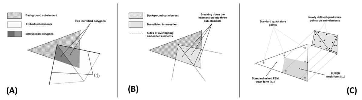
Figure 3: The intersection of one background element and two embedded elements at different stages of computing the PUFEM weak form. (A) Identifying the intersection polygons. B Creating a new tessellation for the overlap area. (C) Defining new set quadrature points for the sub-elements and re-evaluating the basis functions.

Thus we can separate the construction of $\textit{{A}}_{bb}$ into two stages: first building a Laplacian block using classic FEM and second subtracting the classic weak form from the overlap area and replacing it with the PUFEM version. While the former is trivial, the later is more challenging as the fields and integration area are defined on non-matching meshes. In order to overcome this, we construct an intersection or tertiary mesh of sub-elements which allows us relate the background and embedded meshes. Thus, at the start of the second stage, for each background element we want to identify all potentially intersecting embedded elements. This can be achieved optimally by adapting one of several approaches found in the literature [59, 60, 61]. We then test the pairs of background and embedded candidates for intersection and we identify the area of overlap, see Fig. 3. If the area is non-zero, then the resulting intersection will be a convex polygon with up to 6 sides. Each area is subdivided into up to 4 subelements using a Delauney triangulation algorithm and these are stored in the tertiary mesh. The quality of this new mesh is not relevant since it is used for integration exclusively. To finalize the process, we loop over the intersection mesh and we update the block by subtracting the overlap classic weak form and replacing it with the PUFEM one.

Both $\textit{{A}}_{be}$ and $\textit{{A}}_{eb}$ are defined exclusively on $\Omega_{e}$ and thus do not require the first stage introduced $\textit{{A}}_{bb}$. Since both are defined using fields from both meshes, the blocks are constructed by looping over the intersection mesh. In the case of $\textit{{A}}_{ee}$, the block can built using the classic approach due to matching topologies for the space and fields.

The B blocks are generated following an analogous procedure.

3 A PUFEM approach to ALE Navier-Stokes and FSI problems

Building on the foundations of Section 2, in this section, we present the application of PUFEM in the case of more complex settings, namely for ALE Navier-Stokes and FSI problems. Similarly to the Stokes flow case, we begin with a short review of the classic ALE approach (Section 3.1), followed by a presentation of the PUFEM version (Section 3.3), where the focus is on how the method is adapted to deal with having a transient overlap between the two meshes. Finally, in Section 3.5 we outline a method of coupling the fluid solver with a hyper-elastic solid problem.

3.1 Classic FEM approach to the ALE Navier-Stokes problem

Let us consider a time dependent physical domain $\Omega_{f}\subset\mathbb{R}^{d}\times\left[0,T\right]$. At each time point $t\in[0,T]$, we use the $\Omega_{f}(t)$ notation to refer to the current spatial configuration of the fluid domain and let boundary $\Gamma(t)$ be its boundary. We also define the reference domain $\Lambda_{f}\subset\mathbb{R}^{d}$ which can be bijectively mapped to $\Omega_{f}(t)$, for all $t\in\left[0,T\right]$. Hence, $\mathcal{P}:\Lambda_{f}\times\left[0,T\right]\rightarrow\Omega_{f}$ denotes a mapping function used to relate the reference and spatial domains. The non-conservative incompressible Navier-Stokes equation in arbitrary Lagrangian-Eulerian (ALE) form can be written as follows [11, 62]: find $(\textbf{v},p)$ such that

$$\rho\partial_{t}\textbf{v}+\rho(\textbf{v}-\hat{\textbf{v}})\cdot\nabla\textbf{v}-\nabla\cdot\boldsymbol{\sigma}_{f} =\mathbf{0} \text{ in }\Omega_{f}(t),$$ (18a)

$$\nabla\cdot\textbf{v} =0 \text{ in }\Omega_{f}(t),$$ (18b)

v $$=\textbf{v}_{D} \text{ on }\Gamma_{f}^{D}(t),$$ (18c)

v $$=\textbf{v}_{S} \text{ on }\Gamma_{fs}^{D}(t),$$ (18d)

$$\boldsymbol{\sigma}_{f}\cdot\textbf{n} =\textbf{t}_{N} \text{ on }\Gamma^{N}_{f}(t),$$ (18e)

$$\textbf{v}(\cdot,0) =\textbf{v}_{0} \text{ in }\Omega_{f}(0),$$ (18f)

for all $t\in\left[0,T\right]$. Compared to the Stokes flow in (1), the fluid model is augmented with a series of additional elements. The stress tensor is replaced by the symmetric Cauchy stress tensor:

$$\boldsymbol{\sigma}_{f}(\textbf{v})=\mu\left(\nabla\textbf{v}+\nabla\textbf{v}^{T}\right)-p\textit{{I}}$$ (19)

Inertial effects are introduced using the time derivative and nonlinear advection terms. The $\partial_{t}(\cdot)$ operator is the time derivative with respect to a fixed point in $\Lambda_{f}$. The ALE advection term is used to account for the arbitrary motion of the domain, where the arbitrary domain velocity field is defined as $\hat{\textbf{v}}=\partial_{t}\mathcal{P}$ [62, 11]. Finally, we continue to assume that $\textbf{t}_{n}=\mathbf{0}$.

Using BDF(2) discretization, the classic non-conservative FEM problem for equation (18) at a given time step $n$ can be written as [62]: find $(\textbf{v}^{h}_{n},p^{h}_{n})\in\boldsymbol{\mathcal{V}}^{h}_{D}\times\mathcal{W}^{h}$ such that $\forall\hskip 2.84526pt(\textbf{w}^{h},q^{h})\in\boldsymbol{\mathcal{V}}^{h}_{0}\times\mathcal{W}^{h}$ we have

$$\int_{\Omega_{f}^{h}(t_{n})}\rho\left[\frac{3\textbf{v}^{h}_{n}-4\textbf{v}_{n-1}^{h}+\textbf{v}_{n-2}^{h}}{2\Delta t}+\left(\textbf{v}^{h}_{n}-\hat{\textbf{v}}^{h}_{n}\right)\cdot\nabla\textbf{v}_{n}^{h}\right]\cdot\textbf{w}^{h}\hskip 2.84526ptd\Omega+$$

$$\int_{\Omega_{f}^{h}(t_{n})}\boldsymbol{\sigma}_{f}(\textbf{v}^{h}):\nabla\textbf{w}^{h}+q^{h}\nabla\cdot\textbf{v}^{h}_{n}\hskip 2.84526ptd\Omega= 0$$ (20)

Here, we consider the $\textbf{v}_{n-1}^{h},\textbf{v}_{n-2}^{h}\in\boldsymbol{\mathcal{V}}^{h}$ to be the velocity fields at times $t_{n-1}$ and $t_{n-2}$, respectively, which have been transported via ALE mapping into the current spatial configuration.

Due to the non-linearity of the system, we approximate the solution using a Newton-Raphson (NR) based algorithm [63, 64]. The problem is solved semi-monolithically in that the mesh velocity field, $\hat{\textbf{v}}^{h}_{n}$, is solved separately. If $\textbf{v}_{s}$ is provided analytically or is obtained from a weakly-coupled solid solver, then this process can be done at the beginning of each time step. If the fluid and solid solvers are coupled in a monolithic system, then the mesh velocity is recomputed prior to each NR iteration in order to account for the current estimate of the solid deformation.

3.2 Computing mesh velocity

The deformation of the mesh can be determined by an arbitrary problem which is guided by the known deformations on portions of the boundary. It is also well known that the choice of the problem can significantly impact mesh quality over time. For this reason, we propose to propagate the deformation of the boundary onto the entire mesh by solving a solid mechanics problem based on the nearly-incompressible neo-Hookean material model. In order to prevent an excessive deterioration of the mesh we consider the material to be heterogeneous as we allow each element to stiffen in a squared inverse relationship with a metric of its relative element quality. A similar idea has been successfully implemented in [65].

Let us consider the case where we want to compute the mesh deformation for time $n$. We choose $\Lambda_{f}$ to be the reference undeformed domain. Thus the solid problem can be written as follows: find the arbitrary domain deformation field $\hat{\textbf{u}}$ such that

$$\nabla_{0}\cdot\textit{{P}}_{g} =\mathbf{0} \text{in }\Lambda_{f},$$ (21a)

$$\hat{\textbf{u}} =\hat{\textbf{u}}_{D} \text{on }\Gamma^{D}_{ref},$$ (21b)

$$\textit{{P}}_{g}\cdot\textit{{N}} =\mathbf{0} \text{on }\Gamma^{N}_{ref}.$$ (21c)

This relates to the domain deformation velocity as $\hat{\textbf{v}}=\partial_{t}\hat{\textbf{u}}$. Here, the $(0)$ subscript indicates that the divergence operator is defined in the Lagrangian coordinates and the first Piola-Kirchhoff tensor $(\textit{{P}}_{g})$ is given as:

$$\textit{{P}}_{g}=\mu_{g}\left[\frac{1}{J}\left(\textit{{F}}-\frac{\textit{{F}}:\textit{{F}}}{2}\textit{{F}}^{-T}\right)+\kappa J(J-1)\textit{{F}}^{-T}\right]$$ (22)

where $\textit{{F}}=\nabla_{0}\hat{\textbf{u}}$ is the deformation gradient and $J=\det(\textit{{F}})$. The heterogeneous stiffness parameter , $\mu_{g}$, is defined as:

$$\mu_{g}(\tau)=\mu_{ref}\left(\frac{Q(\tau_{0})}{Q(\tau)}\right)^{2}\hskip 14.22636pt\text{ where }\hskip 14.22636ptQ(\tau)=\frac{r}{R}$$

Here $\mu_{ref}$ is the reference stiffness; $Q:\mathcal{T}\rightarrow\mathbb{R}_{+}$ is an element quality metric defined as the ratio between the incircle ($r$) and circumcircle ($R$) of input triangular element; $\tau_{0}$ and $\tau$ denote the original and current shape of the element, respectively. As the quality of the element deteriorates, $Q(\tau)$ decreases, making it stiffer and, thus, less likely to further deform. $\kappa=10$ is a penalty factor on volumetric deformation. This choice was done heuristically and it aims to penalize excessive decreases in element size.

In the discrete time setting, we chose to use the previous time step configuration as the reference, undeformed domain. For the normalization factor $Q(\tau_{0})$, we use the element at time zero as our reference. Given a discrete time point $t_{n}$, we use the deformation field to compute the current space mapping function follows:

$$\mathcal{P}^{h}(\textbf{{X}}^{h},t_{n})=\mathcal{P}^{h}(\textbf{{X}}^{h},t_{n-1})+\hat{\textbf{u}}_{n}^{h}(\textbf{{X}}^{h})$$ (23)

Based on this, the mesh velocity is defined as $\hat{\textbf{v}}^{h}_{n}=\frac{\hat{\textbf{u}}_{n}^{h}}{\Delta t}$.

3.3 PUFEM approach to the ALE Navier-Stokes problem

In Section 2.2 we discussed the setup of PUFEM for flow around a rigid solid. Now we expand these original concepts in order to treat the case where the two meshes are allowed to move independently from each other.

A key requirement for the extension of PUFEM to ALE is the treatment of the material time derivative. Let $\Lambda_{b}^{h}$ and $\Lambda_{e}^{h}$ be the two reference domains for the background and embedded components. $\mathcal{P}_{b}:\Lambda_{b}^{h}\times\left[0,T\right]\rightarrow\Omega_{b}^{h}$ and $\mathcal{P}_{e}:\Lambda_{e}^{h}\times\left[0,T\right]\rightarrow\Omega_{e}^{h}$ are the two arbitrary mapping functions, where $\Omega_{b}^{h}$, $\Omega_{e}^{h}\in\mathbb{R}^{d}\times[0,T]$ are the respective physical domains. We also introduce the $\partial^{b}_{t}(\cdot)$ and $\partial^{e}_{t}(\cdot)$ as the partial time derivatives with respect to fixed points the global and embedded reference domains, respectively. For ease, we consider the ALE expansion of the material time derivative on an arbitrary semi-discrete (in space) scalar field $f^{h}(t)\in\textbf{{V}}^{h}$ which can be written in PUFEM form as $f^{h}=(1-\psi^{h})f^{h}_{b}+\psi^{h}f^{h}_{e}$, where $f_{k}^{h}(t)\in V^{h}_{k,*}$, $k\in\{e,b\}$. Based on this, we can split the time material derivative of $f$ into three terms:

$$\frac{Df^{h}}{Dt}=\frac{D\left[(1-\psi^{h})f_{b}^{h}+\psi^{h}f_{e}^{h}\right]}{Dt}=(1-\psi^{h})\frac{Df_{b}^{h}}{Dt}+\psi^{h}\frac{Df_{e}^{h}}{Dt}+(f_{e}^{h}-f_{b}^{h})\frac{D\psi^{h}}{Dt}$$

Furthermore, we choose $\Lambda_{b}^{h}$ to be the reference domain of $f_{b}^{h}$ and $\Lambda_{e}^{h}$ for $f_{e}^{h}$ and $\psi^{h}$.

Thus, we can continue to expand the first term into its ALE form such that:

$$\left.\frac{Df_{b}^{h}}{Dt}\right|_{\textbf{x}} =\left.\frac{\partial f_{b}^{h}}{\partial t}\right|_{\textbf{x}}+\textbf{v}^{h}\cdot\nabla f_{b}^{h}=\left(\partial^{b}_{t}f_{b}^{h}-\frac{\partial\mathcal{P}^{h}_{b}}{\partial t}\cdot\nabla f_{b}^{h}\right)+\textbf{v}^{h}\cdot\nabla f_{b}^{h}$$

$$=\partial^{b}_{t}f_{b}^{h}+(\textbf{v}^{h}-\hat{\textbf{v}}_{b}^{h})\cdot\nabla f_{b}^{h}$$

Similarly, we also get:

$$\left.\frac{Df_{e}^{h}}{Dt}\right|_{\textbf{x}}=\partial_{t}^{e}f_{e}^{h}+\left(\textbf{v}^{h}-\hat{\textbf{v}}_{e}^{h}\right)\cdot\nabla f_{b}^{h}\hskip 14.22636pt\text{and}\hskip 14.22636pt\left.\frac{D\psi^{h}}{Dt}\right|_{\textbf{x}}=\left(\textbf{v}^{h}-\hat{\textbf{v}}_{e}^{h}\right)\cdot\nabla\psi^{h}$$

In the last case, we assumed that $\partial_{t}^{e}\psi^{h}=0$. The total material time derivative can thus be expressed as:

$$\frac{Df^{h}}{Dt} =(1-\psi^{h})\partial_{t}^{b}f_{b}^{h}+\psi^{h}\partial_{t}^{e}f_{e}^{h}+\textbf{v}^{h}\cdot\nabla f^{h}$$

$$-(1-\psi^{h})\hat{\textbf{v}}_{b}^{h}\cdot\nabla f_{b}^{h}-\psi^{h}\hat{\textbf{v}}_{e}^{h}\cdot\nabla f_{e}^{h}-(f_{e}^{h}-f_{b}^{h})(\hat{\textbf{v}}_{e}^{h}\cdot\nabla\psi^{h})$$

Moving to the discrete form, let us define $\Omega^{h}_{b,n}$ and $\Omega^{h}_{e,n}$, the global and embedded meshes, respectively, for a given time step $n$. Given that $\textbf{{X}}^{v}_{b}$, $\textbf{{X}}^{v}_{e}$, $\textbf{{X}}^{p}_{b}$ and $\textbf{{X}}^{p}_{e}$ change with the alignment of the meshes with respect to each other at each time step, let us define $\textbf{{V}}^{h}_{D,n}$, $\textbf{{V}}^{h}_{0,n}$ and $W^{h}_{n}$ as the test and trial spaces at discrete time $t_{n}$. Thus the new discrete weak form of the ALE Navier-Stokes problem can be written as follows: find $(\textbf{v}^{h}_{n},p^{h}_{n})\in\textbf{{V}}^{h}_{D,n}\times W^{h}_{n}$ such that for any $(\textbf{w}^{h},q^{h})\in\textbf{{V}}^{h}_{0,n}\times W^{h}_{n}$ we have that

$$\int_{\Omega^{h}_{b}(t_{n})}\rho\left(\frac{3\textbf{v}^{h}_{n}-4\textbf{v}^{h}_{n-1}+\textbf{v}^{h}_{n-2}}{2\Delta t}+\textbf{v}^{h}_{n}\cdot\nabla\textbf{v}^{h}_{n}\right)\cdot\textbf{w}^{h}~{}d\Omega+$$

$$\int_{\Omega^{h}_{b}(t_{n})}-\rho\left[(1-\psi^{h}_{n})(\hat{\textbf{v}}^{h}_{b,n}\cdot\nabla)\textbf{v}^{h}_{b,n}+\psi^{h}_{n}(\hat{\textbf{v}}^{h}_{e,n}\cdot\nabla)\textbf{v}^{h}_{e}\right]\cdot\textbf{w}^{h}\hskip 2.84526ptd\Omega+$$

$$\int_{\Omega^{h}_{b}(t_{n})}-\rho(\hat{\textbf{v}}^{h}_{e}\cdot\nabla\psi^{h}_{n})(\textbf{v}^{h}_{e,n}-\textbf{v}^{h}_{b,n})\cdot\textbf{w}^{h}+\boldsymbol{\sigma}^{h}_{f,n}:\nabla\textbf{w}^{h}-q^{h}\nabla\cdot\textbf{v}^{h}_{n}~{}d\Omega= 0$$ (24)

where $\textbf{v}^{h}_{n}=(1-\psi^{h})\textbf{v}^{h}_{b,n}+\psi^{h}\textbf{v}^{h}_{e,n}$. Both partial derivatives $\partial^{g}_{t}(\cdot)$ and $\partial^{e}_{t}(\cdot)$ have been approximated using the BDF(2) scheme. In order to solve this system of equations, we again employ the technique described in [64] and [63]. The structure of the resulting Jacobian matrix is largely based on that of system matrix described in Eq. (14). The changes arise in the sub-block A where in addition to the Laplacian we also have mass and advection terms resulting from linearisation of the residual:

$$\left(\textit{{A}}^{ij}_{bb}\right)_{MN} =\int_{\Omega^{h}_{b,n}}\rho\delta_{ij}\left[\frac{3}{2\Delta t}\psi^{h}_{b}\psi^{h}_{b}\hat{\phi}^{M}_{v}\hat{\phi}^{N}_{v}+\psi^{h}_{b}\hat{\phi}^{M}_{v}\left(\textbf{v}_{n}^{h}\cdot\nabla\right)\left(\psi^{h}_{b}\hat{\phi}^{N}_{v}\right)\right]~{}d\Omega$$

$$+\int_{\Omega^{h}_{b,n}}\rho\psi^{h}_{b}\psi^{h}_{b}\left[\hat{\phi}^{M}_{v}\hat{\phi}^{N}_{v}\frac{\partial\left(\textbf{v}^{h}_{n}\right)_{i}}{\partial x_{j}}-\delta_{ij}\hat{\phi}^{M}_{v}\left(\hat{\textbf{v}}^{h}_{b,n}\cdot\nabla\right)\hat{\phi}^{h}_{v}\right]~{}d\Omega$$

$$-\int_{\Omega^{h}_{b,n}}\rho\delta_{ij}\hat{\phi}^{M}_{v}\hat{\phi}^{N}_{v}\left(\hat{\textbf{v}}^{h}_{e}\cdot\nabla\psi^{h}_{b}\right)-\mu\delta_{ij}\nabla\left(\psi^{h}_{b}\hat{\phi}^{M}_{v}\right):\nabla\left(\psi^{h}_{b}\hat{\phi}^{N}_{v}\right)~{}d\Omega$$

$$+\int_{\Omega^{h}_{b,n}}\mu\frac{\partial\psi^{h}_{b}\hat{\phi}^{M}_{v}}{\partial x_{j}}\frac{\partial\psi^{h}_{b}\hat{\phi}^{N}_{v}}{\partial x_{i}}~{}d\Omega$$ (25)

The other blocks resulting from permutations of background/embedded test and trial functions are obtained analogously. Here, $i$ and $j$ correspond to the spatial orientation of test and trial DOF, respectively. $M$ and $N$ represent the indexes of the mesh nodes. For ease, $\psi^{h}_{b}$ is used as shorthand for $(1-\psi^{h})$. The application of Dirichlet boundary conditions and additional constraints is largely the same as the one described in Section 2.2. The exception is that while the Jacobian is re-used for multiple time iterations, the constraints such as $\textbf{v}_{b}=\textbf{x}_{e}$ for $\textbf{x}\in\textbf{{X}}^{v}_{b}$ need to be re-adjusted based on the new overlap configuration.

3.4 Transient fixed nodes in ALE context

Moving the background and embedded meshes independently from each other introduces new challenges: having a different area of overlap in consecutive time steps and, by extension, having transient sets $\textbf{{X}}^{v}_{b}$ and $\textbf{{X}}^{p}_{b}$. While the latter is of less importance, the former can be significant factor of instability due to the need to use previous time step solutions in order to approximate the velocity time derivative, as shown in Eq. 24. Thus, if a node is fixed at one time $t_{n}$ and subsequently active at time $t_{n+2}$, our estimation of the acceleration is dependent on what we chose to assign $t_{n}$. While, this concern has been partly addressed in Section 2.2.1, it only covers the case of background nodes which are found under the fluid area of the embedded mesh. Thus, in this case we can assign them a meaningful value through interpolation. This leaves, however, the case of background nodes found under the solid. Here there are two scenarios. In the first case our area of enrichment is sufficiently thick and the time step is sufficiently small such that when a background node, after it leaves solid, remains in the overlap area for at least two more time steps. This would allow for sufficient time for the node to obtain meaningful data in order to compute the derivative. However, this would be difficult to control, particularly in FSI. An alternative solution that we propose is to constrain the value of background nodes in the solid to be equal to the interpolated solid velocity field, which is generally continuous to that of the fluid flow. If this field is provided or is computed as part of the FSI solution, then this new task is trivial. If however, only the surface motion is provided, one can potentially create a field by solving an artificial problem, such as a diffusion one. It should be noted though that this last approach is only theoretical and was never implemented for this work.

3.5 PUFEM for FSI

To illustrate the efficacy of the PUFEM approach for FSI, in this section we elaborate on a monolithic approach to coupling the ALE Navier-Stokes solver described in Section 3.3 with a generic quasi-static non-linear solid. Let $\Omega_{s,0}$ and $\Omega_{s,t}\subset\mathbb{R}^{d}$ be our reference and deformed (at time $t$) solid domains. Thus, the strong form of the FSI and ALE mesh problems can be written as: find $(\textbf{v}_{f},p_{f},\textbf{u}_{s},p_{s},\hat{\textbf{u}}_{e})$ such that

$$\begin{aligned} \rho\partial_{t}\textbf{v}_{f}+\rho(\textbf{v}_{f}-\hat{\textbf{v}})\cdot\nabla\textbf{v}_{f}-\nabla\cdot\boldsymbol{\sigma}_{f}&\\ \nabla\cdot\textbf{v}_{f}&\\ \textbf{v}_{f}&\\ \boldsymbol{\sigma}_{f}\cdot\textbf{n}&\\ \textbf{v}_{f}(\cdot,0)&\end{aligned} \begin{aligned} &=\mathbf{0}\\ &=0\\ &=\textbf{v}_{f,D}\\ &=\textbf{t}_{f,N}\\ &=\textbf{v}_{0}\end{aligned} \begin{aligned} &\text{in }\Omega_{f},\\ &\text{in }\Omega_{f},\\ &\text{on }\Gamma_{f}^{D}\\ &\text{on }\Gamma^{N}_{f},\\ &\text{in }\Omega_{f,0},\end{aligned}$$ (26)

$$\begin{aligned} \nabla_{0}\cdot\textit{{P}}_{s}(\textbf{u}_{s},p_{s})&\\ J-1&\\ \textbf{u}_{s}&\\ \textit{{P}}_{s}(\textbf{u}_{s},p_{s})\cdot\textit{{N}}&\end{aligned} \begin{aligned} &=\mathbf{0}\\ &=0\\ &=\textbf{u}_{s,D}\\ &=\textbf{t}_{s,N}\end{aligned} \begin{aligned} &\text{in }\Omega_{s,0}\\ &\text{in }\Omega_{s,0}\\ &\text{on }\Gamma^{D}_{s,0}\\ &\text{on }\Gamma^{N}_{s,0}\end{aligned}$$ (27)

$$\begin{aligned} \boldsymbol{\sigma}_{f}\cdot\textbf{n}+J^{-1}\textit{{P}}_{s}(\textbf{u}_{s},p_{s})\cdot\textit{{N}}&\\ \textbf{v}_{f}&\\ \end{aligned} \begin{aligned} &=\mathbf{0}\\ &=\dot{\textbf{u}}_{s}\\ \end{aligned} \begin{aligned} &\text{on}~{}\Gamma_{\mathit{fs}}\\ &\text{on}~{}\Gamma_{\mathit{fs}}\\ \end{aligned}$$ (28)

$$\begin{aligned} \nabla_{0}\cdot\textit{{P}}_{g}(\hat{\textbf{u}}_{e})&\\ \hat{\textbf{u}}_{e}&\\ \textit{{P}}_{g}(\hat{\textbf{u}}_{e})\cdot\textit{{N}}&\end{aligned} \begin{aligned} &=\mathbf{0}\\ &=\textbf{u}_{f}\\ &=\mathbf{0}\end{aligned} \begin{aligned} &\text{in }\Omega_{e,0}\\ &\text{on }\Gamma_{\mathit{fs},0}\\ &\text{on }\Gamma_{\mathit{ff},0}\end{aligned}$$ (29)

The FSI problem can be divided into four parts: the fluid problem in (26), the quasi-static solid problem in (27), the coupling conditions in (28) and the ALE mesh problem in (29). For illustrative purposes, we chose to use the neo-Hookean model for the solid, resulting in the following form of the first Piola-Kirchhoff stress tensor:

$$\textit{{P}}_{s}=\frac{\mu_{s}}{J_{s}}\left[\textit{{F}}_{s}-\frac{\textit{{F}}_{s}:\textit{{F}}_{s}}{2}\textit{{F}}_{s}^{-T}\right]-p_{s}J_{s}\textit{{F}}_{s}^{-T}$$ (30)

where $\textit{{F}}_{s}=\nabla_{0}\textbf{u}_{s}$ and $J_{s}=det(\textit{{F}}_{s})$. Note, we chose to simplify the solid problem by considering the loading process to be quasi-static. The constitutive law used for the arbitrary mesh deformation problem has been previously described in Section 3.2. The PUFEM discrete setting is elaborated on in the next section.

3.5.1 Discrete weak form

The main difference compared to the ALE Navier-Stokes set-up described in Section 3.3 is that now we also need to solve the deformation/translation of the solid, rather than it being given. In order to take advantage of the definition of the PUFEM spaces in (7), (10) and (9) which extend into both $\Omega_{f}^{h}$ and $\Omega_{s}^{h}$, for each time step we compute the solid’s velocity $\textbf{v}^{h}_{n}$, rather than its displacement. The deformation is obtained using the backward Euler scheme ($\textbf{u}^{h}_{s,n}=\textbf{u}^{h}_{s,n-1}+\textbf{v}^{h}_{s,n}\Delta t$). Thus, the problem coupling is ensured by the fact that the fluid and solid velocity DOF are identical on $\Gamma_{fs}$.

The fully discrete weak form can be written as: find $(\textbf{v}^{h}_{n},p_{n}^{h})\in\textbf{{V}}^{h}_{D,n}\times W^{h}_{n}$ such that $\forall\hskip 2.84526pt(\textbf{w}^{h},q^{h})\in\textbf{{V}}^{h}_{0,n}\times W^{h}_{n}$

$$\int_{\Omega^{h}_{f,n}}\rho\left(\frac{3\textbf{v}^{h}_{n}-4\textbf{v}^{h}_{n-1}+\textbf{v}^{h}_{n-2}}{2\Delta t}+\textbf{v}^{h}_{n}\cdot\nabla\textbf{v}^{h}_{n}\right)\cdot\textbf{w}^{h}~{}d\Omega +$$

$$\int_{\Omega^{h}_{f,n}}-\rho\left[\left(1-\psi^{h}_{n}\right)\hat{\textbf{v}}_{b,n}^{h}\cdot\nabla\textbf{v}^{h}_{b,n}+\psi^{h}_{n}\hat{\textbf{v}}^{h}_{e,n}\cdot\nabla\textbf{v}^{h}_{e,n}\right]\cdot\textbf{w}^{h}\hskip 2.84526ptd\Omega +$$

$$\int_{\Omega^{h}_{f,n}}-\rho(\hat{\textbf{v}}^{h}_{e}\cdot\nabla\psi^{h}_{n})(\textbf{v}^{h}_{e,n}-\textbf{v}^{h}_{b,n})\cdot\textbf{w}^{h}\hskip 2.84526ptd\Omega +$$

$$\int_{\Omega^{h}_{f,n}}\boldsymbol{\sigma}_{f,n}^{h}:\nabla\textbf{w}^{h}_{n}+q^{h}\nabla\cdot\textbf{v}^{h}_{n}\hskip 2.84526ptd\Omega +$$

$$\int_{\Omega^{h}_{s,0}}\textit{{P}}_{s}:\nabla_{0}\textbf{w}^{h}+q^{h}(J_{s}-1)\hskip 2.84526ptd\Omega =0$$ (31)

The structure of the system of equations which has to be solved during each Newton-Raphson remains largely the same. Note, the pressure is allowed to be discontinuous across $\Gamma_{\mathit{fs}}$

3.6 Implementation

In order to examine the performance of PUFEM against the classic mixed FEM technique, we implemented both approaches in the MATLAB 2017b language. The meshes used for the test were produced using the MESH2D package [66, 67]. All the simulation where run on MacBook pro 2017 running on macOS Sierra, with an Intel Core i7-7820HQ processors and 16 GB of 2133 MHz LPDDR3 RAM.

4 Numerical Results

4.1 Stokes flow convergence test

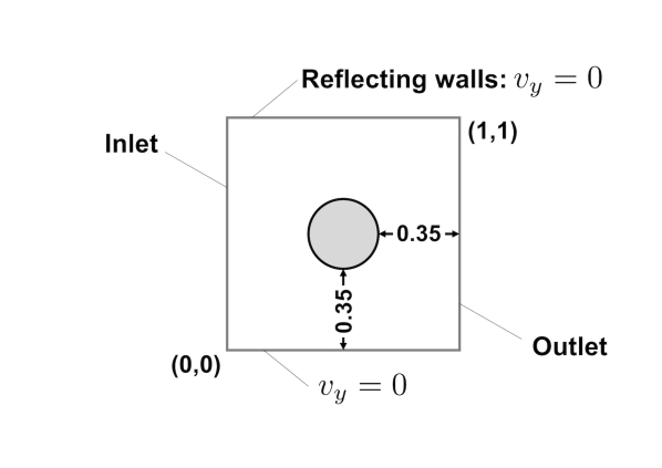
Figure 4: Domain used in the steady-state Stokes and Navier-Stokes problems.

In order to illustrate the comparable accuracy of PUFEM to that of standard boundary fitted FEM, we consider a basic steady-state incompressible Stokes flow problem, where we compute the errors in the velocity and pressure fields on series of meshes. More specifically, we consider a total domain $\Omega_{f}\cup\Omega_{s}=\left[0,1\right]^{2}$ where a rigid cylindrical obstacle (with a radius of 0.15) is placed in the centre, see Fig. 4. The inflow (left side) is constrained using the Dirichlet condition, $\textbf{v}_{inflow}=[1;0]^{T}$, which is constant throughout the boundary patch. On the side walls, we apply a reflection Dirichlet condition on the velocity field, such that $v_{y}=0$, and on the outflow we impose a zero traction condition. Fluid viscosity was set to 1.0. The purpose of this arrangement is to concentrate the boundary layer flow to the vicinity of cylinder, which coincides with the area enriched by the embedded mesh.

To ease comparison, we try to use meshes with small variations in element size. For both approaches, we consider five refinement levels, with $h$ ranging from approximately $0.1$ to $0.00625$. In the case of PUFEM we paired the background and embedded meshes such that $h_{g}\approx h_{e}$. The latter mesh is composed of two regions: the cylinder, which is only used to define the solid surface, and the fluid enrichment area, which forms a ring with a thickness 0.161. We shall refer to this grid as M1. More details about their statistics and that of the classic mesh set can be found in Table 1.

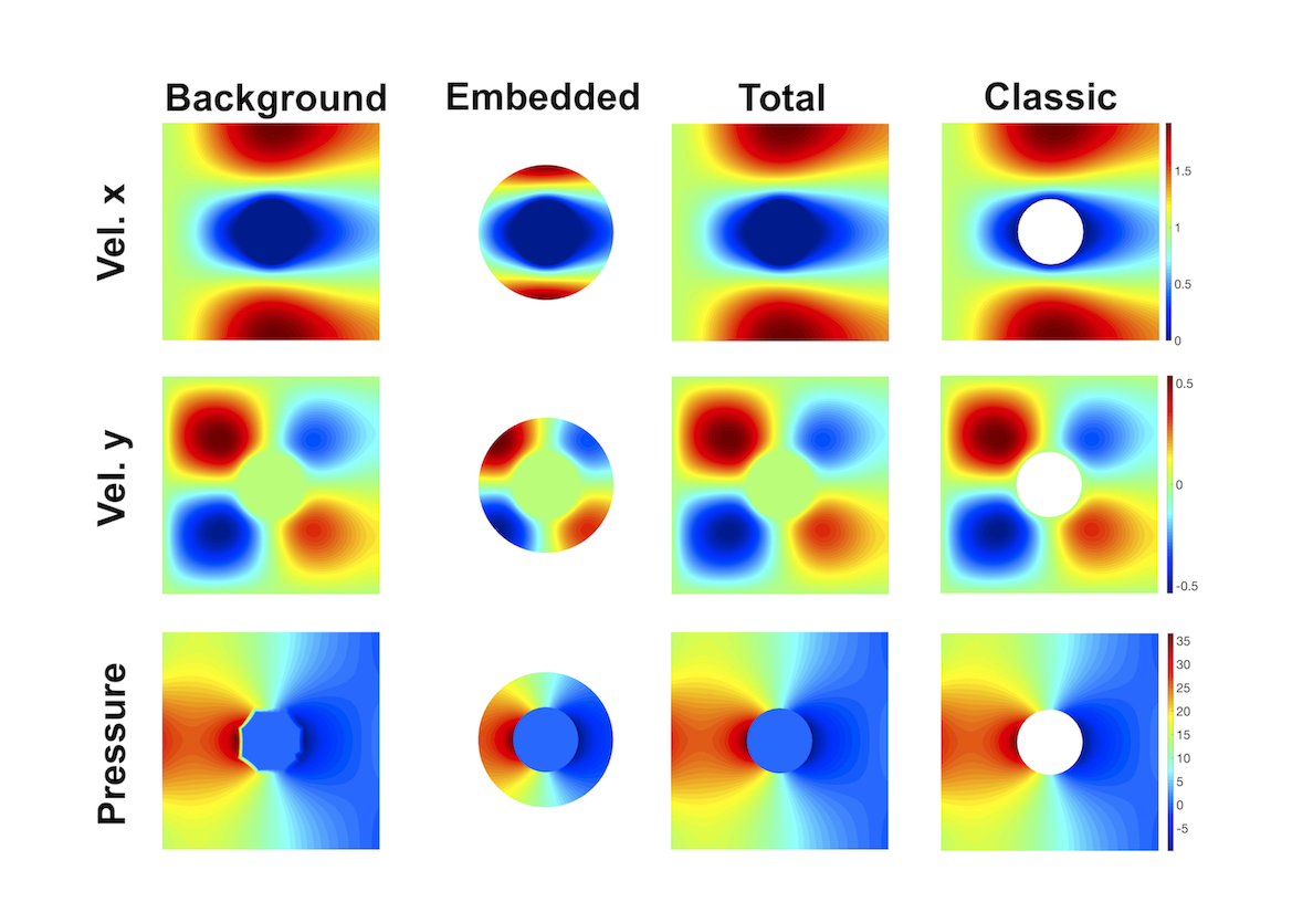
Figure 5: Example of solution fields for the Stokes problem obtained using the PUFEM and classic approaches. The PUFEM figures include the background and embedded components, as well as the total (resulting from the weighted sum).

The resulting velocity and pressure fields and their subcomponents can be seen in Fig. 5. The PUFEM weighted sum result and the classic solution appear to be very similar. Additionally, there are no obvious non-physical behaviours, such as field jumps, which might have been generated by the coupling.

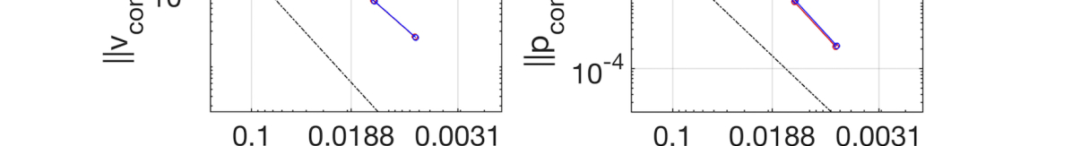
Figure 6: Plot showing the errors in the velocity and pressure fields for the Stokes flow problem obtained with the classical and PUFEM approaches. The dotted line indicates the optimal convergence rate.

The results of the convergence test are shown in Fig.  6. Note, that we did not rely on an analytical reference solution to compute the error. In order to obtain a reference, the flow field was computed using the classic approach and a very fine, boundary fitted grid with an element size of $h=0.0016$. We observe that velocity and pressure fields seem to converge in the case of both PUFEM and boundary fitted approach, with rates which closely follow the the a priori estimate in Eq. 6. We observe that the velocity produces slightly suboptimal results, however, this is likely due to both projection errors and non-conformity between solutions. We also notice that the difference in errors across the approaches are very small. Given the mesh size similarity among the methods, PUFEM was not expected to exceed the performance of the classical approach. Thus, the accuracy of the new method is ultimately capped by the local approximation capability of the background and embedded grids. Furthermore, the coupling, representing the main potential error source, appears to have little deteriorating impact.

4.2 Steady-state Navier-Stokes convergence test

To examine PUFEM performance for steady-state Navier-Stokes, we consider the problem outlined in Fig 4 for Reynolds numbers of 30 and 100. We keep using the $[0,1]^{2}$ domain with $R=0.15$ cylindrical obstacle in the middle. The fluid parameters are set to: $\rho=1.0$ and $\mu=0.01$. The boundary conditions are kept largely the same with the exception of the inflow velocity. Thus, the $x$ direction component is set to $1.0$ or $10/3$, depending on whether we want to compute the $Re$ 30 or 100 cases. Again, our errors estimates are based on flow results computed using the classic approach and a fine grid with $h=0.0016$. This test allows us to look at any potential deterioration in the accuracy of PUFEM due to introduction of non-linearity. Moreover, by increasing the Reynolds number we reduce the size of the boundary layer, which enables us to better assess the benefit of using the embedded mesh to enrich the total solution space. For PUFEM, we introduce a second mesh set, denoted M2, where $h_{b}\approx 2h_{e}$. See Table 1 for the corresponding mesh statistics.

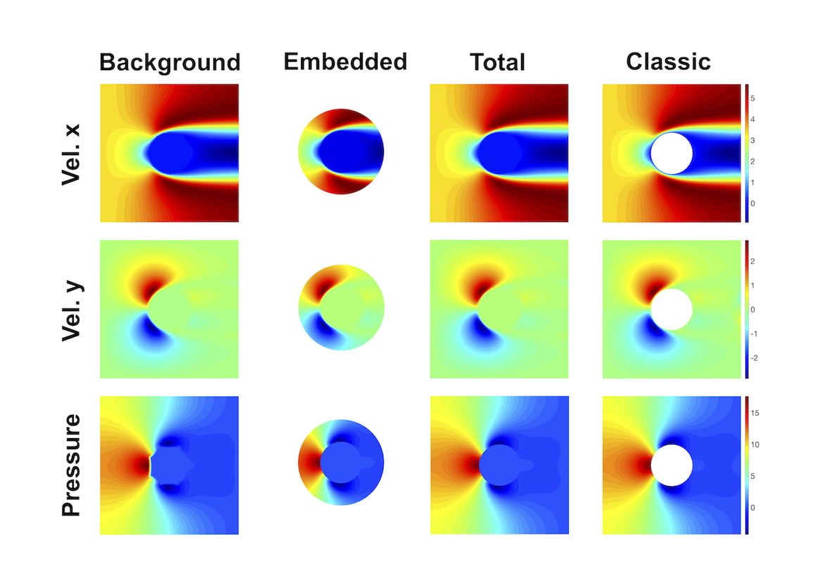
Figure 7: Example of solution fields for the Navier Stokes problem at $Re$ 100 obtained using the PUFEM and classic approaches. The PUFEM figures include the background and embedded components, as well as the total (resulting from the weighted sum).

A set of sample results for the velocity and pressure at $Re$ 100 can be seen in Fig. 7. Despite the increase in flow complexity, the quality of the PUFEM solution remains comparable to that of the classic result.

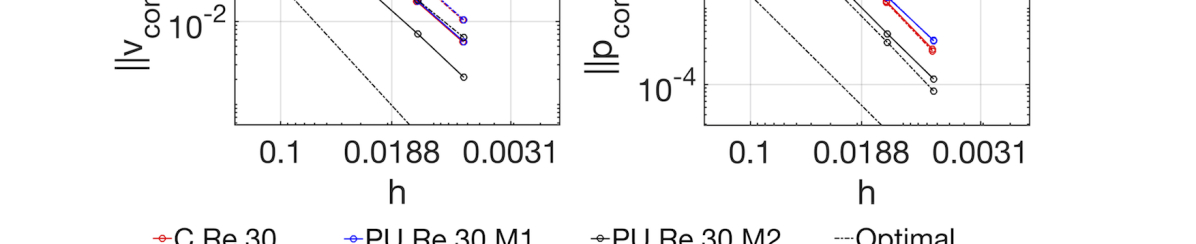
Figure 8: The error plots for steady state incompressible Navier-Stokes. Both classic (C) and PUFEM (PU) methods are run at Reynolds number of 30 and 100.

The error plots for the different cases are found in Fig. 8. A first observation is that the convergence behaviour for $Re$ 30 and 100 remains relatively unchanged from that observed in Stokes flow problem. Furthermore, the differences in accuracy between classic and PUFEM (M1) approaches remain small. As previously noted in the Stokes case, when using similar spatial discretization, we do not expect the new approach present a significant advantage. It continues to perform well in these circumstances and is seemingly unaffected by the rise in $Re$. Switching to M2, we see an overall decrease in error. This suggest that PUFEM can potentially leverage local solution enrichment to improve overall accuracy. While a similar behaviour can be replicated in the case of boundary fitted grids using adaptive meshing, the main strength of the new method resides in its ability to better withstand large deformations.

4.3 Schäfer-Turek benchmark

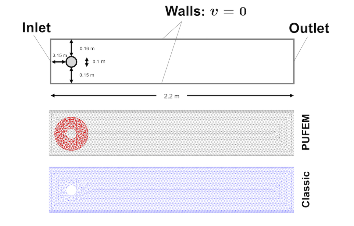
Figure 9: The domain of the Schäfer-Turek benchmark problem with boundary labels as well as example meshes used in PUFEM and classic approaches.

In order to evaluate the stability of the PUFEM method in the case of time dependent problems and also to compare it to other published flow results, we considered the Schäfer-Turek benchmark [68], case 2D-2 with $Re=100$ (see Fig. 9).

The inflow constraint is imposed on the velocity using the following Dirichlet condition:

$$\textbf{v}=\left[\begin{array}[]{c}\frac{4Uy(W-y)}{W^{2}}\min(t,1)\\ 0\end{array}\right]$$

After linearly ramping up, the inflow profile remains constant and we run the problem for $10$ $s$ in simulation time, enough to initiate the characteristic shedding and also to reach steady state oscillations. Here $U=1.5~{}m/s$ is the reference flow speed and $W=0.41~{}m$ is the width of the tube. We also impose a no slip condition on the side walls and zero traction on the outflow. In order to achieve the correct Reynolds number, density ($\rho$) and viscosity ($\mu$) are set to $1~{}kg/m^{3}$ and $0.001~{}Pa\cdot s$, respectively.

In total, six solutions are produced using PUFEM based on two mesh sets (PU1 and PU2) and three time steps (i.e. 0.01, 0.002 and 0.001 $s$). Each mesh set consists of a regular background grid and a boundary fitted embedded grid. The fluid region of the latter forms a ring with a thickness of 0.1 $m$ around the cylinder, see Fig. 9. For simplicity, each set uses a constant $h$ for both background and embedded grids, with the value set to 0.025 and 0.0125 $cm$ in the case of PU1 and PU2, respectively. Additional mesh statistics are found in Table 2. To aid the comparison, we have also produced a set of flow results using the classical approach using a quasi-regular grid with $h=0.025$ and a time step of 0.01 $s$.

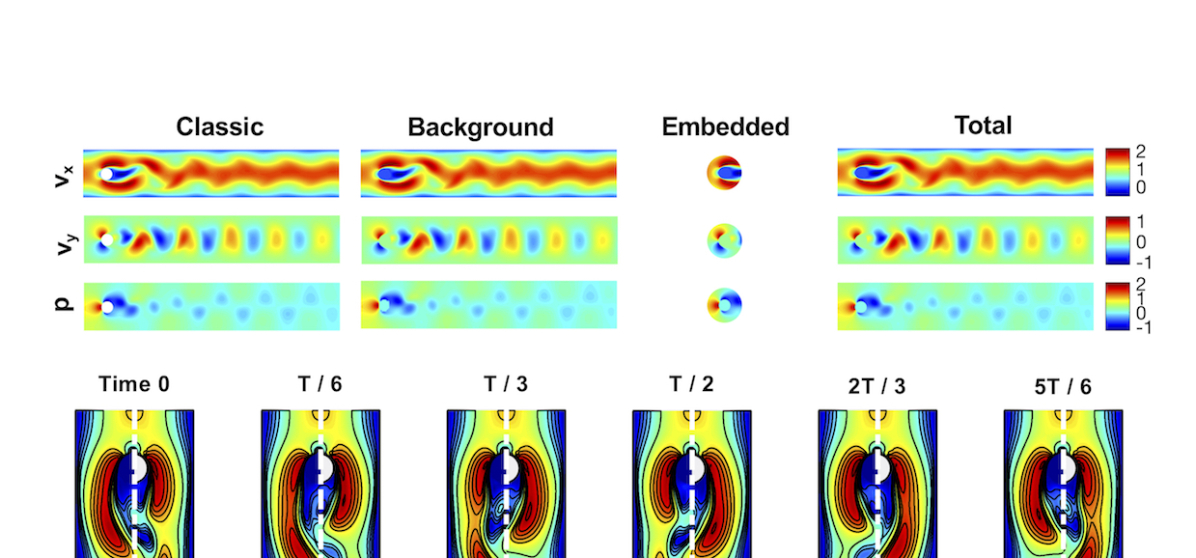
Figure 10: Compiled results for the Turek benchmark. (Top) A breakdown of the PUFEM solution at peak $c_{l}$ (9.57 $s$ in simulation time) into background, embedded and total fields for each component of the solution. The classic result is introduced for comparison. (Bottom) Velocity magnitude over a cycle in both PUFEM and classical simulations. Contour lines where added to aid comparison.

Fig. 10 shows an example set of flow results (i.e. velocity components and pressure) computed using classic and PUFEM approaches. In the top part, we have a snapshot of the flow at one of the time points of maximum lift (i.e. 9.57 $s$ in simulation time for PUFEM). The results are split into subcomponents corresponding to the boundary fitted mesh, background, embedded meshes and the weighted sum. In the second half of the figure, we include six velocity magnitude snapshots at the different stages of the shedding process. Each frame is split in two, with the right side showing the PUFEM field and the left displaying the classic, showing the wake patterns are in good agreement. Furthermore, the transition between the embedded and background grids retains its smoothness, despite the transient behaviour of the solution.

From a quantitative perspective, we also computed the coefficients of drag ($c_{d}$), lift ($c_{l}$), Strouhal number($St$) and pressure drop across the cylinder ($\Delta p$), defined as:

$$c_{d} =\frac{2F_{d}}{\rho\bar{U}^{2}D},\hskip 14.22636ptF_{d}=\int_{\Gamma_{\mathit{fs}}}\mu\frac{\partial v_{t}}{\partial n}n_{y}-pn_{x}~{}d\Gamma$$

$$c_{l} =\frac{2F_{l}}{\rho\bar{U}^{2}D},\hskip 14.22636ptF_{l}=-\int_{\Gamma_{\mathit{fs}}}\mu\frac{\partial v_{t}}{\partial n}n_{x}+pn_{y}~{}d\Gamma$$

$$St =\frac{fD}{\bar{U}},$$

where $D$ is the diameter and $v_{t}$ is the tangential fluid velocity. These values have been compiled in Table 3, which contains all the PUFEM and classic results, as well as those from literature. For similar space and time discretization, i.e. entries two and three of the table, the new and classic approaches provide similar estimations of the with errors of: $0.03\%$ for $c_{d}$, $0.22\%$ for $c_{l}$, $3\%$ for $St$, and $0.16\%$ for $\Delta p$. By comparing to the literature values [68], we see that the PUFEM estimations of $St$ and $\Delta p$ are converging inside the recommended interval. However, $c_{d}$ and $c_{l}$ are generally underestimated, with minimum errors of $1.18\%$ and $1.41\%$, respectively, achieved using the PU2 mesh set and 5000 time steps. Generally, though, the trend suggests that all four parameters would converge provided sufficient spatial and temporal discretization.

Given the initial stage of the development, it has not been our aim to produce an optimal implementation of PUFEM. However, this has represented a significant obstacle to running very large problems. For example, the total solving time for the classic and new approaches using the mesh sets FEM1 and PU1, respectively, and a time step of 0.01 $s$ were approx. 1.9 and 2.9 hours, respectively. In this case, where the mesh overlap is fixed, the main factor responsible PUFEM’s lag appears to be the residual’s assembly, with an average running time 0.42 $s$, compared to 0.097 $s$ for the classic. While not addressed in this work, there are multiple avenues which could be used to reduce the this disparity: restricting the interface mesh to the area where $\psi$ is strictly between 0 and 1, contracting this area to a thinner strip close to $\Gamma_{\mathit{ff}}^{h}$ and optimizing the quadrature rule being used, to name a few.

4.4 ALE: An oscillating rigid cylinder

Moving towards moving domain applications, we define a simple ALE benchmark problem. Using a similar to setup to that of the Turek benchmark, we now place the cylinder in the middle of the domain, and we oscillate it along the long axis of the tube, while we allow for free outflow at the left and right ends. The cylinder displacement as a function of time is defined as:

$$d(t)=\left\{\begin{array}[]{cc}A\frac{\sin(\omega t)}{\omega}-At\text{ }\cos(\omega t),&t\leq 1\\ -A\text{ }\cos(\omega t),&t>1\end{array}\right.$$ (32)

where $A$ is the maximum amplitude and $\omega$ is the frequency. We chose to set $A~{}=~{}0.2$ m and $\omega=2\pi\hskip 2.84526pts^{-1}$ , resulting in a maximum velocity of approx $1.25\hskip 2.84526ptms^{-1}$ and a $Re\approx 100$. We are interested in the first 2 seconds of the simulations. The goal of this test is to verify the stability of the PUFEM approach in the context of a transient overlap area. For this reason, the amplitude of the displacement was chosen large enough to cause multiple sharp changes in $\Omega_{cut}$.

For the spatial discretization, we define a new ALE-PU1 mesh set to be consistent with the new geometry (i.e. in accordance to the repositioned cylinder) and with identical mesh statistics as PU1 (i.e. due to recycled connectivity matrices). For the classical approach, a new boundary fitted mesh (ALE-FEM1) was constructed with 14708 elements and $h=2.5\text{ cm}$. A step size of $\Delta t=0.01~{}s$ was used for the temporal discretization.

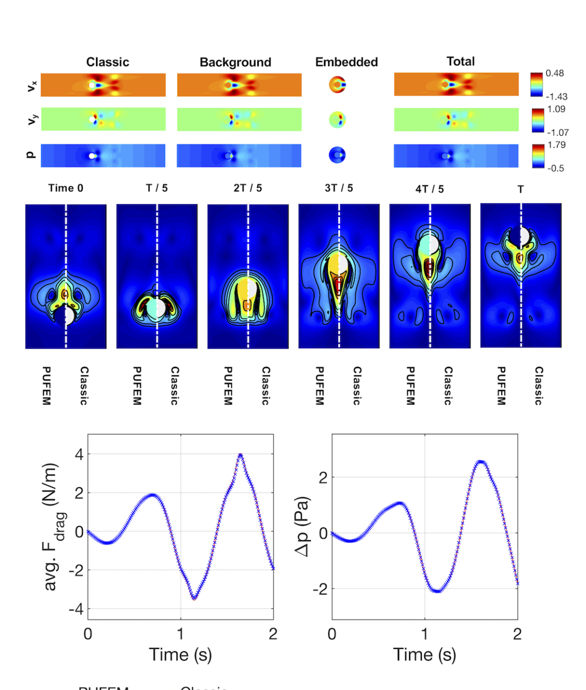
Figure 11: Compiled results for the ALE problem. (Top) A breakdown of the PUFEM solution into background(global), embedded and total. Classical result is introduced for comparison. (Middle) The $x$ component of the velocity as it evolves between the two points of maximum displacement from the centre. Contour lines were added to aid comparison. (Bottom) Estimated drag force and pressure difference across the cylinder for the PUFEM and classical (BF1) methods.

For a qualitative comparison between methods, we maintained the same format for displaying the flow results as in the case of the Schäfer-Turek benchmark, see Fig. 11. The top part of the figure is a snapshot at $t=2\hskip 2.84526pts$ showing the velocity components and pressure field as computed on the boundary fitted, the background and embedded grids. The corresponding PUFEM total field is also included. The middle part displays snapshots of the velocity magnitude at different stages of a transition from right to left. In general, the two methods seem to be in agreement, with only minor differences. In contrast to previous examples, the ALE problem is the first case in this work which includes the concept of transient fixed nodes, see Fig. 12 .Thus, the good quality of our solution now also suggests the effectiveness of using the interpolation strategy on providing nodes with a meaningful solution while they are temporarily fixed.

We also computed the mean surface drag force ($F_{d}$) and pressure across the left and right ends of the cylinder ($\Delta p$). Fig. 11 (bottom) shows the values of these coefficients at all time points of the simulation. The maximum overall errors that we obtain are $4.0\%$ for the mean $F_{d}$ and $0.8\%$ for $\Delta p$. Potential sources which may influence the error (excluding PUFEM) include mesh deterioration in the case of the classic approach and also the fact that we did not aim to minimize the errors through spatial and temporal refinement. Despite this, these results suggest that PUFEM can be used in an ALE context to obtain reasonably accurate estimations of surface stresses and pressure experienced by the solid. This quality is particularly relevant in the case FSI, where the balance of tractions is part of the coupling conditions.

4.5 Valve simulation

To examine the suitability of PUFEM for FSI applications, we present an example of an idealised 2D aortic valve, see Fig. 13. The FSI domain consists of two components: one half of the lumen and one leaflet. In order to reduce computation cost, we assume to have rigid aortic walls and symmetry along the long axis. We also do not include coronary flow. The fluid is modelled as an incompressible Navier-Stokes fluid, while the solid is assumed to behave as an incompressible neo-Hookean material [69]. The main domain characteristics and constitutive law parameters can be found in Table 4. At the inflow we impose a single pulse with parabolic a profile:

$$\textbf{v}(y,t)=\left[\begin{array}[]{c}V_{max}\frac{y(2W-y)}{W^{2}}\sin^{2}(\pi t)\\ 0\end{array}\right]$$ (33)

where $V_{max}=0.5\text{ }m/s$ is the maximum velocity, $W$ is the width of the inflow and $y$ is the spatial coordinate. The total in-simulation duration is $T=1\text{ }s$, or one pulse, which we discretise using constant time steps of $\Delta t=0.01\text{ }s$. Thus we can observe, the flow fields both during valve deflection as well as relaxation. On the surface of the wall and leaflet we impose a no-slip condition, while on the long axis we apply a symmetry condition. For the outflow, we impose a zero traction Neumann condition.

In order to reduce the element deterioration and the loss of accuracy which may derive from it, the mesh used in the classic approach is built as follows. First, a mesh is constructed on the reference domain and we run the simulation up to the $t_{mid}=0.15\text{ }s$. The time point was chosen heuristically in order to capture the configuration of the domain during mid valve deflection. This data is then used to construct a second mesh. Using the connectivity matrix of this grid, a final mesh is defined by interpolating the $t=0.15\text{ }s$ node coordinates onto the space at $t=0\text{ }s$. Thus, the classic grid is comprised of 8248 elements, with mean and maximum $h$ values of $0.4$ mm and $2.8mm$, respectively.

For PUFEM, the two grids are generated in the initial domain configuration. We used a background mesh with 4380 element and an average $h$ of 0.7 mm. The embedded grid is formed of 844 elements with mean $h$ of 0.5 mm.

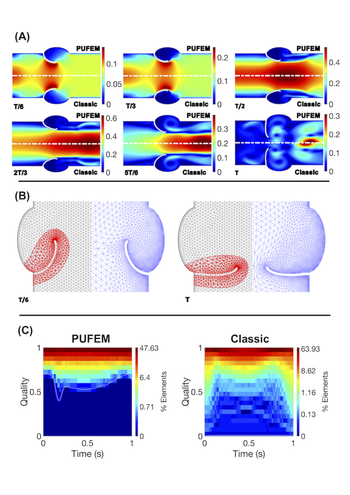
Figure 14: (A) Six snapshots of the velocity magnitude as computed by the PUFEM and classical approaches. (B) The PUFEM and ALE mesh setups at the medium and minimum mesh deflection. At minimum deflection, the ALE mesh reaches a point of almost maximum deterioration. (C) The distribution in time of elements as a function of quality for both approaches.

The main flow results are summarized in Fig. 14: the velocity magnitude fields at different stages of the pulse (A); the grid deformation at half-way deflection and end time point (B); and the element quality distribution as it evolves in time (C). From a qualitative perspective, the flow physics appear to be quite similar at all time stages. While significant differences appear in the second part of the simulation, we believe that these are generally due to a combination of the grid deterioration in the case of the classic approach and decelerating flows, which are more sensitive to its effects. In fact, without the use midway meshing, to try to attenuate these effects, we observed much more striking difference between methods (results not shown here). The deterioration of grid quality for the classic approach can be clearly seen in (B). Thus, while at $T/6$ (midway deflection), the boundary fitted mesh typically displays good quality elements, at $T$ (end of relaxation) many of the elements close to the tip of the leaflet appear to be squeezed against the axis of symmetry. On the other hand PUFEM does not show such clear signs, suggesting that mesh can undergo even more significant deformation. This is also reflected in (C), where for PUFEM’s embedded grid the minimum element quality only temporarily drops bellow 0.5. In the case of the classic approach, the element population is selected from the interval $[1.5,3.7]$ cm on the $x$ axis, as shown in (B). Here we see that while a majority number of elements retains an excellent quality, for many the value is very low, close to collapsing. The reason for having a much wider population spread at the start and end of the simulation is a result of using the midway meshing strategy. In return, the population appears to be much more skewed towards one in the middle half of the simulation, when the we experience the highest inflow velocity.

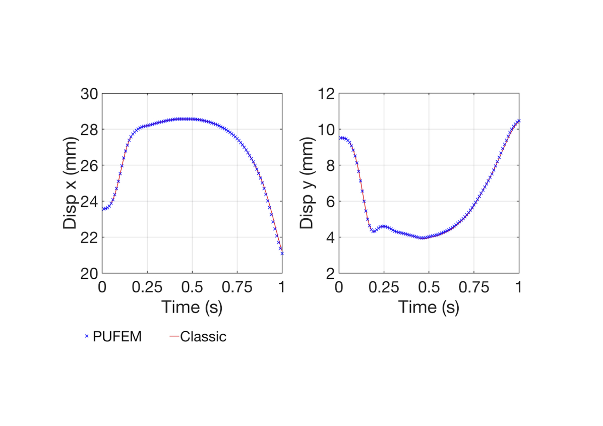
Figure 15: The $x$ and $y$ displacements of the valve tip as it evolved in the classic and PUFEM approaches. The reference nodes where chosen such that they have identical coordinates at $t=0~{}s$.

From the solid mechanics perspective, a good agreement can also be observed for the valve tip deflection, see Fig. 15, with maximum absolute errors of $0.21$ and $0.1\text{ }mm$ in $x$ and $y$ directions, respectively.

Combined, these preliminary results on FSI suggest not only show a good level of accuracy for PUFEM, comparable to that of the classic approach, but also to a greater degree of flexibility, where we can better retain element quality while undergoing significant mesh deformation.

5 Conclusion

In this work we have presented a novel approach to solving fluid flow and FSI problems based on the partition of unity (PUFEM). Thus, the total flow solution is defined as weighted sum of background and embedded fields. The weighting field, which is defined on the embedded mesh, is used to facilitate a smooth transition between areas where the solution is dominated by one mesh or the other.

The accuracy and stability of the method has been assessed on a range of 2D tests with an increasing level complexity. For comparison, all tests were replicated using a classic boundary fitted FEM approach which served as our golden standard. Using steady-state results for flow around the cylinder, we showed that PUFEM displayed nearly optimal convergence rates for both Stokes and Navier-Stokes, and that the the accuracy of the two approaches is nearly indistinguishable for similar spatial discretization. This suggests that PUFEM can leverage the approximation power of both meshes with little deterioration as a result of the coupling process.

In the case of the Schäfer-Turek, the flow results produced by PUFEM where shown to be in good agreement with the classic approach. Additionally, the estimation of surface stresses, pressure and wake frequency appeared to be in accord with literature values.

To assess the accuracy and stability of PUFEM in the ALE setting, we designed a problem where flow is generated in an open-ended channel by an oscillating, rigid cylinder. The method appeared robust to the changing of the overlapping area and the set of constrained nodes. Additionally, a good agreement was maintained between approaches in the estimation of surface drag forces and pressure drop.

An idealised aortic valve FSI problem was chosen for testing of realistic applications. Given the set up the problem, the resulting flow is complex with the occurrence of recirculation and small vortexes during relaxation. In addition to displaying a high level of similarity between the physical behaviour obtained using the two approaches, we where able to gauge the evolution of mesh quality over the course of the simulation. Thus, the use of overlapping meshes appears to produce the desired effect of reducing the well known mesh degradation associated with large deformations.

Combined, these results indicate the potential applicability of PUFEM to a wide range of FSI applications, allowing for boundary fitted fluid-solid interface and targeted solution space enrichment, in the absence of the need for re-meshing or the need for user-defined stabilization parameters.

Future work will focus on providing a theoretical analysis on the stability and convergence of the PUFEM solver. Other extensions of this work will include porting it into a parallel 3D implementation [70] and the study of different approaches to include contact mechanics.

Additional Information

Declarations of interest: none.

References

	Level 1	Level 2	Level 3	Level 4	Level 5
Classic
h	0.1	0.05	0.025	0.0125	$0.1/2^{4}$
element no.	225	880	3488	13774	54746
nodes (P1)	136	488	1840	7079	27757
M1	Level 1	Level 2	Level 3	Level 4	Level 5
$h$	0.1	0.05	0.025	0.0125	$0.1/2^{4}$
B. element no.	232	926	3704	14816	59264
E. element no.	76	296	1196	4454	17310
B. nodes (P1)	137	504	1933	7569	29953
E. nodes (P1)	48	166	630	2295	8789
M2
Background $h$	0.1	0.05	0.025	0.0125	$0.1/2^{4}$
Embedded $h$	0.05	0.025	0.0125	$0.1/2^{4}$	$0.1/2^{5}$
E. element no.	296	1196	4454	17310	69110
E. nodes (P1)	166	630	2295	8789	34822

Table 1: Statistics corresponding to the mesh sets used in the steady Stokes and Navier-Stokes convergence tests.

	FEM	PUFEM
Label	FEM1	PU1		PU2
		Background	Embedded	Background	Embedded
Elements	14684	14816	1106	56362	4390
DOF	67208	67745	5189	255742	20171
${h}$ (cm)	2.5	2.5	2.5	1.25	1.25

Table 2: Number of elements, DOF and average element size for the meshes used in the Turek benchmark.

	Time steps	$c_{d}$	$c_{l}$	$St$	$\Delta p$
Lit. [68]	-	$3.22-3.24$	$0.99-1.01$	$0.295-0.305$	$2.46-2.50$
FEM1	1000	$3.054$	$0.906$	$0.2941$	$2.4950$
PU1	1000	$3.053$	$0.904$	$0.3030$	$2.4911$
PU1	2000	$3.060$	$0.926$	$0.3030$	$2.4981$
PU1	5000	$3.061$	$0.929$	$0.3030$	$2.4988$
PU2	1000	$3.175$	$0.950$	$0.2941$	$2.4801$
PU2	2000	$3.179$	$0.970$	$0.3030$	$2.4870$
PU2	5000	$3.182$	$0.976$	$0.3030$	$2.4820$

Table 3: Coefficient estimates from PUFEM and classic FEM for the Turek benchmark.

Figure 12: An example of transient fixed nodes on the background mesh. The red arrows point to free nodes, while the blue ones point to their constrained counterpart at different time. The element colour coding indicates the following: element cut by $\Gamma^{h}_{\mathit{ff}}$ (deep grey), element completely weighed out by $\psi^{h}$ (light grey).

Domain dimensions
	Inflow width	Max width	Aortic length	Sinus length	Valve height
Distance (mm)	14	17.9	55.3	15.8	9.8
Fluid parameters			Solid parameters
$\mu_{f}\text{ }(Pa\cdot s)$	$3\times 10^{-3}$		$\mu_{s}\text{ }(Pa\cdot s)$	$20\times 10^{3}$
$\rho\text{ }(kg/m^{3})$	1030

Table 4: (Top) The main domain dimensions in the aortic valve problem. (Bottom) The constitutive law parameters for the fluid and solid problems.

Figure 13: (Left) Illustration of the fluid and valve domains used in the FSI test. A summary of the domain dimensions is found in Table 4. (Right) The meshes used in the classic and PUFEM approaches. For visualization purposes the solid mesh was excluded.

References

- [1] K. Stein, R. Benney, V. Kalro, A. Johnson, T. Tezduyar, K. Stein, R. Benney, V. Kalro, A. Johnson, T. Tezduyar, Parallel computation of parachute fluid-structure interactions, in: 14th Aerodynamic Decelerator Systems Technology Conference, 1997, p. 1505.
- [2] V. Kalro, T. E. Tezduyar, A parallel 3D computational method for fluid–structure interactions in parachute systems, Computer Methods in Applied Mechanics and Engineering 190 (3-4) (2000) 321–332.
- [3] K. Takizawa, T. Spielman, T. E. Tezduyar, Space–time FSI modeling and dynamical analysis of spacecraft parachutes and parachute clusters, Computational Mechanics 48 (3) (2011) 345.
- [4] Y. Bazilevs, M.-C. Hsu, I. Akkerman, S. Wright, K. Takizawa, B. Henicke, T. Spielman, T. Tezduyar, 3D simulation of wind turbine rotors at full scale. Part I: Geometry modelling and aerodynamics, International Journal for Numerical Methods in Fluids 65 (1-3) (2011) 207–235.
- [5] Y. Bazilevs, M.-C. Hsu, J. Kiendl, R. Wüchner, K.-U. Bletzinger, 3D simulation of wind turbine rotors at full scale. Part II: Fluid–structure interaction modelling with composite blades, International Journal for Numerical Methods in Fluids 65 (1-3) (2011) 236–253.
- [6] M.-C. Hsu, D. Kamensky, F. Xu, J. Kiendl, C. Wang, M. C. Wu, J. Mineroff, A. Reali, Y. Bazilevs, M. S. Sacks, Dynamic and fluid–structure interaction simulations of bioprosthetic heart valves using parametric design with T-splines and Fung-type material models, Computational mechanics 55 (6) (2015) 1211–1225.
- [7] H. Gao, L. Feng, N. Qi, C. Berry, B. E. Griffith, X. Luo, A coupled mitral valve–left ventricle model with fluid–structure interaction, Medical engineering & physics 47 (2017) 128–136.
- [8] M. McCormick, D. Nordsletten, P. Lamata, N. P. Smith, Computational analysis of the importance of flow synchrony for cardiac ventricular assist devices, Computers in biology and medicine 49 (2014) 83–94.
- [9] K. Lau, V. Diaz, P. Scambler, G. Burriesci, Mitral valve dynamics in structural and fluid–structure interaction models, Medical engineering & physics 32 (9) (2010) 1057–1064.
- [10] B. Baillargeon, I. Costa, J. R. Leach, L. C. Lee, M. Genet, A. Toutain, J. F. Wenk, M. K. Rausch, N. Rebelo, G. Acevedo-Bolton, et al., Human cardiac function simulator for the optimal design of a novel annuloplasty ring with a sub-valvular element for correction of ischemic mitral regurgitation, Cardiovascular engineering and technology 6 (2) (2015) 105–116.
- [11] Y. Bazilevs, K. Takizawa, T. E. Tezduyar, Computational fluid-structure interaction: methods and applications, John Wiley & Sons, 2013.
- [12] A. Verkaik, M. Hulsen, A. Bogaerds, F. van de Vosse, An overlapping domain technique coupling spectral and finite elements for fluid flow, Computers & Fluids 100 (2014) 336–346.
- [13] C. W. Hirt, A. A. Amsden, J. Cook, An arbitrary Lagrangian-Eulerian computing method for all flow speeds, Journal of computational physics 14 (3) (1974) 227–253.
- [14] J. Donea, S. Giuliani, J.-P. Halleux, An arbitrary Lagrangian-Eulerian finite element method for transient dynamic fluid-structure interactions, Computer methods in applied mechanics and engineering 33 (1-3) (1982) 689–723.
- [15] T. J. Hughes, W. K. Liu, T. K. Zimmermann, Lagrangian–Eulerian finite element formulation for incompressible viscous flows, Computer methods in applied mechanics and engineering 29 (3) (1981) 329–349.
- [16] R. Van Loon, P. Anderson, F. Van de Vosse, S. Sherwin, Comparison of various fluid–structure interaction methods for deformable bodies, Computers & structures 85 (11-14) (2007) 833–843.
- [17] T. E. Tezduyar, S. Sathe, Modelling of fluid–structure interactions with the space–time finite elements: solution techniques, International Journal for Numerical Methods in Fluids 54 (6-8) (2007) 855–900.
- [18] A. M. Bavo, G. Rocatello, F. Iannaccone, J. Degroote, J. Vierendeels, P. Segers, Fluid-structure interaction simulation of prosthetic aortic valves: comparison between immersed boundary and arbitrary Lagrangian-Eulerian techniques for the mesh representation, PloS one 11 (4) (2016) e0154517.
- [19] R. Glowinski, T.-W. Pan, J. Periaux, A fictitious domain method for Dirichlet problem and applications, Computer Methods in Applied Mechanics and Engineering 111 (3-4) (1994) 283–303.
- [20] R. Glowinski, T.-W. Pan, T. I. Hesla, D. D. Joseph, A distributed Lagrange multiplier/fictitious domain method for particulate flows, International Journal of Multiphase Flow 25 (5) (1999) 755–794.
- [21] I. Babuška, The finite element method with Lagrangian multipliers, Numerische Mathematik 20 (3) (1973) 179–192.
- [22] L. Zhang, A. Gerstenberger, X. Wang, W. K. Liu, Immersed finite element method, Computer Methods in Applied Mechanics and Engineering 193 (21-22) (2004) 2051–2067.
- [23] L. Zhang, M. Gay, Immersed finite element method for fluid-structure interactions, J. Fluids Struct. 23 (6) (2007) 839–857.
- [24] D. Boffi, N. Cavallini, L. Gastaldi, The finite element immersed boundary method with distributed lagrange multiplier, SIAM J. Numer. Anal. 53 (6) (2015) 2584–2604.
- [25] D. Boffi, L. Gastaldi, A fictitious domain approach with lagrange multiplier for fluid-structure interactions, Numer. Math. 135 (3) (2017) 711–732.
- [26] A. J. Gil, A. A. Carreño, J. Bonet, O. Hassan, The immersed structural potential method for haemodynamic applications, Journal of Computational Physics 229 (22) (2010) 8613–8641.
- [27] N. D. Dos Santos, J.-F. Gerbeau, J.-F. Bourgat, A partitioned fluid–structure algorithm for elastic thin valves with contact, Computer Methods in Applied Mechanics and Engineering 197 (19-20) (2008) 1750–1761.
- [28] D. Kamensky, M.-C. Hsu, D. Schillinger, J. A. Evans, A. Aggarwal, Y. Bazilevs, M. S. Sacks, T. J. Hughes, An immersogeometric variational framework for fluid–structure interaction: Application to bioprosthetic heart valves, Computer methods in applied mechanics and engineering 284 (2015) 1005–1053.
- [29] R. Van Loon, P. D. Anderson, J. De Hart, F. P. Baaijens, A combined fictitious domain/adaptive meshing method for fluid–structure interaction in heart valves, International Journal for Numerical Methods in Fluids 46 (5) (2004) 533–544.
- [30] A. Gerstenberger, W. A. Wall, An extended finite element method/Lagrange multiplier based approach for fluid–structure interaction, Computer Methods in Applied Mechanics and Engineering 197 (19-20) (2008) 1699–1714.
- [31] F. Alauzet, B. Fabrèges, M. A. Fernández, M. Landajuela, Nitsche-XFEM for the coupling of an incompressible fluid with immersed thin-walled structures, Computer Methods in Applied Mechanics and Engineering 301 (2016) 300–335.
- [32] M. Landajuela, Coupling schemes and unfitted mesh methods for fluid-structure interaction, Ph.D. thesis, Université Pierre et Marie Curie, Paris, France (2016).
- [33] B. Schott, Stabilized cut finite element methods for complex interface coupled flow problems, Ph.D. thesis, Technical University of Munich (2017).
- [34] A. Massing, B. Schott, W. Wall, A stabilized Nitsche cut finite element method for the Oseen problem, Comput. Methods Appl. Mech. Engrg. 328 (2018) 262–300.
- [35] M. Winter, B. Schott, A. Massing, W. Wall, A Nitsche cut finite element method for the Oseen problem with general Navier boundary conditions, Comput. Methods Appl. Mech. Engrg. 330 (2017) 220–252.
- [36] S. Zonca, L. Formaggia, C. Vergara, An unfitted formulation for the interaction of an incompressible fluid with a thick structure via an xfem/dg approach, SIAM J. Sci. Comput. 40 (1) (2016) B59–B84.
- [37] L. Formaggia, C. Vergara, S. Zonca, Unfitted extended finite elements for composite grids, Comput. Math. Appl. 76 (4) (2018) 893–904.
- [38] T. E. Tezduyar, Computation of moving boundaries and interfaces and stabilization parameters, International Journal for Numerical Methods in Fluids 43 (5) (2003) 555–575.
- [39] J. Steger, F. Dougherty, J. Benek, A chimera grid scheme, in: Advances in Grid Generation, Vol. ASME FED-5, 1983, pp. 59–69.
- [40] J. L. Steger, J. A. Benek, On the use of composite grid schemes in computational aerodynamics, Computer Methods in Applied Mechanics and Engineering 64 (1-3) (1987) 301–320.
- [41] G. Chesshire, W. D. Henshaw, Composite overlapping meshes for the solution of partial differential equations, J. Comput. Phys. 90 (1) (1990) 1–64.
- [42] G. Houzeaux, R. Codina, A Chimera method based on a Dirichlet/Neumann(Robin) coupling for the Navier–Stokes equations, Comput. Methods Appl. Mech. Engrg. 192 (31-32) (2003) 3343–3377.
- [43] W. A. Wall, P. Gamnitzer, A. Gerstenberger, Fluid–structure interaction approaches on fixed grids based on two different domain decomposition ideas, International Journal of Computational Fluid Dynamics 22 (6) (2008) 411–427.
- [44] A. Hansbo, P. Hansbo, M. G. Larson, A finite element method on composite grids based on Nitsche’s method, ESAIM: Mathematical Modelling and Numerical Analysis 37 (3) (2003) 495–514.
- [45] A. Massing, M. G. Larson, A. Logg, M. Rognes, A Nitsche-based cut finite element method for a fluid-structure interaction problem, Commun. Appl. Math. Comput. Sci. 10 (2) (2015) 97–120.
- [46] B. Schott, S. Shahmiri, R. Kruse, W. Wall, A stabilized nitsche-type extended embedding mesh approach for 3d low-and high-reynolds-number flows, Int. J. Numer. Methods Fluids.
- [47] A. Koblitz, S. Lovett, N. Nikiforakis, W. D. Henshaw, Direct numerical simulation of particulate flows with an overset grid method, Journal of Computational Physics 343 (2017) 414–431.
- [48] E. Burman, Projection stabilization of lagrange multipliers for the imposition of constraints on interfaces and boundaries, Numerical Methods for Partial Differential Equations (2013) n/a–n/a.
- [49] E. Burman, P. Hansbo, Fictitious domain finite element methods using cut elements: I. A stabilized Lagrange multiplier method, Comput. Methods Appl. Mech. Engrg. 199 (2010) 2680–2686.
- [50] M. Puso, E. Kokko, R. Settgast, J. Sanders, B. Simpkins, B. Liu, An embedded mesh method using piecewise constant multipliers with stabilization: mathematical and numerical aspects, Int. J. Numer. Methods Eng.
- [51] A. Massing, M. G. Larson, A. Logg, M. E. Rognes, A stabilized Nitsche overlapping mesh method for the Stokes problem, Numerische Mathematik 128 (1) (2014) 73–101.
- [52] A. Johansson, M. G. Larson, A. Logg, High order cut finite element methods for the Stokes problem, Advanced Modeling and Simulation in Engineering Sciences 2 (1) (2015) 24.
- [53] J. Nitsche, Über ein Variationsprinzip zur Lösung von Dirichlet-Problemen bei Verwendung von Teilräumen, die keinen Randbedingungen unterworfen sind. InAbhandlungen aus dem mathematischen Seminar der Universität Hamburg 1971 Jul 1 (Vol. 36, No. 1, pp. 9-15).
- [54] J. M. Melenk, I. Babuška, The partition of unity finite element method: basic theory and applications, Computer methods in applied mechanics and engineering 139 (1-4) (1996) 289–314.
- [55] Y. Huang, J. Xu, A conforming finite element method for overlapping and nonmatching grids, Math. Comp. 72 (243) (2003) 1057–1066.
- [56] A. Quarteroni, A. Valli, Numerical approximation of Partial Differential Equations, Springer, 1994, Ch. 9, pp. 297–337.
- [57] V. Girault, P.-A. Raviart, Finite element methods for Navier-Stokes equations: theory and algorithms, Vol. 5, Springer Science & Business Media, 2012.
- [58] C. Taylor, P. Hood, A numerical solution of the Navier-Stokes equations using the finite element technique, Computers & Fluids 1 (1) (1973) 73–100.
- [59] A. Massing, M. G. Larson, A. Logg, Efficient implementation of finite element methods on nonmatching and overlapping meshes in three dimensions, SIAM Journal on Scientific Computing 35 (1) (2013) C23–C47.
- [60] U. M. Mayer, A. Gerstenberger, W. A. Wall, Interface handling for three-dimensional higher-order XFEM-computations in fluid–structure interaction, International Journal for Numerical Methods in Engineering 79 (7) (2009) 846–869.
- [61] K. Wang, J. Grétarsson, A. Main, C. Farhat, Computational algorithms for tracking dynamic fluid–structure interfaces in embedded boundary methods, International Journal for Numerical Methods in Fluids 70 (4) (2012) 515–535.
- [62] D. Nordsletten, N. Smith, D. Kay, A preconditioner for the finite element approximation to the arbitrary Lagrangian–Eulerian Navier–Stokes equations, SIAM Journal on Scientific Computing 32 (2) (2010) 521–543.
- [63] A. Hessenthaler, O. Röhrle, D. Nordsletten, Validation of a non-conforming monolithic fluid-structure interaction method using phase-contrast MRI, International journal for numerical methods in biomedical engineering 33 (8) (2017) e2845.
- [64] V. Shamanskii, A modification of Newton’s method, Ukrainian Mathematical Journal 19 (1) (1967) 118–122.
- [65] J. H. Spühler, J. Jansson, N. Jansson, J. Hoffman, 3D Fluid-Structure Interaction Simulation of Aortic Valves Using a Unified Continuum ALE FEM Model, Frontiers in physiology 9.
- [66] D. Engwirda, Unstructured mesh methods for the Navier-Stokes equations, Undergraduate Thesis, School of Engineering, University of Sidney.
- [67] D. Engwirda, Locally optimal Delaunay-refinement and optimisation-based mesh generation, PhD thesis, School of Mathematics and Statistics, University of Sydney.
- [68] Schäfer, Michael and Turek, Stefan and Durst, Franz and Krause, Egon and Rannacher, Rolf, Benchmark computations of laminar flow around a cylinder, in: Flow simulation with high-performance computers II, Springer, 1996, pp. 547–566.
- [69] M. Hadjicharalambous, J. Lee, N. P. Smith, D. A. Nordsletten, A displacement-based finite element formulation for incompressible and nearly-incompressible cardiac mechanics, Computer methods in applied mechanics and engineering 274 (2014) 213–236.
- [70] J. Lee, A. Cookson, I. Roy, E. Kerfoot, L. Asner, G. Vigueras, T. Sochi, S. Deparis, C. Michler, N. P. Smith, et al., Multiphysics computational modeling in CHeart, SIAM Journal on Scientific Computing 38 (3) (2016) C150–C178.