Vison Crystals in an Extended Kitaev Model on the Honeycomb Lattice

Abstract

We introduce an extension of the Kitaev honeycomb model by including four-spin interactions that preserve the local gauge structure and hence the integrability of the original model. The extended model has a rich phase diagram containing five distinct vison crystals, as well as a symmetric $\pi$-flux spin liquid with a Fermi surface of Majorana fermions and a sequence of Lifshitz transitions. We discuss possible experimental signatures and, in particular, present finite-temperature Monte Carlo calculations of the specific heat and the static vison structure factor. We argue that our extended model emerges naturally from generic perturbations to the Kitaev honeycomb model.

Introduction. The famous Kitaev model on the honeycomb lattice Kitaev (2006) is an exactly solvable yet experimentally realistic model of a quantum spin liquid. In contrast to more conventional magnetic phases, quantum spin liquids retain extensive (quantum) fluctuations all the way down to zero temperature Balents (2010), where the spins appear to fractionalize into deconfined “spinon” quasiparticles coupled to appropriate gauge fields Savary and Balents (2016).

The Kitaev model is approximately realized in a family of strongly spin-orbit-coupled honeycomb materials, where its anisotropic spin interactions emerge between effective $J=1/2$ angular momenta in the $t_{2g}$ orbitals of $4d$ or $5d$ ions Jackeli and Khaliullin (2009); Rau et al. (2016); Trebst (2017); Hermanns et al. (2018). To determine the most accurate microscopic spin models for these Kitaev materials, including (Na,Li)₂IrO₃ Singh and Gegenwart (2010); Liu et al. (2011); Singh et al. (2012); Choi et al. (2012); Ye et al. (2012); Comin et al. (2012); Hwan Chun et al. (2015); Williams et al. (2016); Kitagawa et al. (2018) and $\alpha$-RuCl₃ Plumb et al. (2014); Sandilands et al. (2015); Sears et al. (2015); Majumder et al. (2015); Johnson et al. (2015); Sandilands et al. (2016); Banerjee et al. (2016); Sears et al. (2017); Banerjee et al. (2017); Baek et al. (2017); Do et al. (2017); Banerjee et al. (2018); Hentrich et al. (2018); Kasahara et al. (2018), various extensions of the Kitaev model have been considered and analyzed with a wide range of techniques Chaloupka et al. (2010); Jiang et al. (2011); Reuther et al. (2011); Price and Perkins (2012); Rau et al. (2014); Yamaji et al. (2014); Sizyuk et al. (2014); Sela et al. (2014); Rousochatzakis et al. (2015); Kim et al. (2015); Yadav et al. (2016); Kim and Kee (2016); Winter et al. (2016); Kim et al. (2016); Janssen et al. (2016); Hou et al. (2017); Winter et al. (2017); Samarakoon et al. (2017); Ran et al. (2017); Samarakoon et al. (2018); Gordon et al. (2019). While these models are experimentally realistic and have rich phase diagrams in the classical limit, it is challenging to identify and characterize quantum phases in them. For a start, the honeycomb lattice may harbor many different quantum spin liquids Lu and Ran (2011); You et al. (2012), and the Kitaev spin liquid, captured by the Kitaev model, is only one among these many candidates. In addition, a quantum spin liquid may also remain “hidden” by appearing on top of classical symmetry-breaking order Savary and Balents (2012).

From a more phenomenological point of view, the low-energy physics of the Kitaev spin liquid is described by Majorana fermions (spinons) with Dirac nodes, coupled to an emergent $\mathbb{Z}_{2}$ gauge field Kitaev (2006). At each plaquette of the honeycomb lattice, the $\mathbb{Z}_{2}$ gauge field may form a $\pi$ flux, corresponding to a “vison” excitation. In turn, the presence of such a vison affects the kinetic energy of the spinons via the Berry phase $\pi$ picked up by each spinon moving around it. For the pure Kitaev model, the spinons are governed by a nearest-neighbor hopping problem (cf. electrons in graphene) and, due to the lack of frustration, the ground state has no visons at any plaquettes Kitaev (2006); Lieb (1994). However, if the hopping problem is frustrated by competing hopping amplitudes, the presence of a vison may reduce the frustration and thus lower the kinetic energy of the spinons. Such a frustration in the hopping amplitudes is known to stabilize crystals of topological solitons, such as baby skyrmions or merons, in itinerant magnets Ozawa et al. (2016); Batista et al. (2016); Ozawa et al. (2017), and one may thus expect it to stabilize analogous vison crystals in the Kitaev spin liquid.

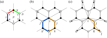
Figure 1: Extended Kitaev model. (a) Honeycomb lattice with two sublattices $A$ and $B$ (black and white dots), three bond types $x$, $y$, and $z$ (red, green, and blue bonds), and the site-labeling convention around a plaquette $p$. (b)-(c) Representative (orange) paths $\langle ijkl\rangle_{yzx}$ (b) and $\langle ijkl\rangle_{yzy}$ (c) associated with the $K_{3}$ and $K_{3}^{\prime}$ terms in Eq. (2), respectively; four-spin interactions along such paths give rise to Majorana hopping from any site $i$ to all its third neighbors not , as indicated by the dashed arrows. For the path $\langle ijkl\rangle_{yzx}$ (b), the symmetry-related path $\langle ij^{\prime}k^{\prime}l\rangle_{xzy}$ is marked by blue.

In this Letter, we extend the Kitaev model by including four-spin interactions that preserve the exact solution of the model and emerge naturally from generic perturbations. By introducing frustrated further-neighbor hopping for the Majorana fermions, these additional interactions stabilize a rich variety of vison crystals, as well as a symmetric $\pi$-flux spin liquid with a vison at every plaquette. Interestingly, the $\pi$-flux spin liquid exhibits a Fermi surface of Majorana fermions undergoing two subsequent Lifshitz transitions. On a technical level, we first use a simple variational treatment to compute the zero-temperature phase diagram of our extended model. The validity of this approach is then confirmed by unbiased Monte Carlo (MC) simulations that also reveal the finite melting temperatures of the vison crystals.

Model. We consider a generalized Kitaev Hamiltonian on the honeycomb lattice:

$${\cal H}={\cal H}_{K_{1}}+{\cal H}_{K_{3}},$$ (1)

where ${\cal H}_{K_{1}}=-K_{1}\sum_{\langle ij\rangle_{\alpha}}\sigma^{\alpha}_{i}\sigma^{\alpha}_{j}$ is the usual Kitaev (2006) isotropic Kitaev Hamiltonian with ferromagnetic ($K_{1}>0$) Ising interactions between the spin components $\sigma^{\alpha}$ along each $\alpha=\{x,y,z\}$ bond $\langle ij\rangle_{\alpha}$ [see Fig. 1(a)], and

$${\cal H}_{K_{3}}=K_{3}\sum_{\langle ijkl\rangle_{\alpha\beta\gamma}}\sigma_{i}^{\alpha}\sigma_{j}^{\gamma}\sigma_{k}^{\alpha}\sigma_{l}^{\gamma}-K_{3}^{\prime}\sum_{\langle ijkl\rangle_{\alpha\beta\alpha}}\sigma_{i}^{\alpha}\sigma_{j}^{\gamma}\sigma_{k}^{\gamma}\sigma_{l}^{\alpha},$$ (2)

where $(\alpha\beta\gamma)$ is a permutation of $(xyz)$ in each term, and $\langle ijkl\rangle_{\alpha\beta\gamma}$ is a path of length $3$ consisting of bonds $\langle ij\rangle_{\alpha}$, $\langle jk\rangle_{\beta}$, and $\langle kl\rangle_{\gamma}$. Each term in ${\cal H}_{K_{3}}$ is the product of the three terms in ${\cal H}_{K_{1}}$ that correspond to the three bonds along the appropriate path. Different $K_{3}$ and $K_{3}^{\prime}$ terms are related by space-group symmetries, simultaneously transforming the lattice and the spins; particular examples of their respective paths, with $(\alpha\beta\gamma)=(yzx)$, are depicted in Figs. 1(b) and 1(c). We remark that, for each path $\langle ijkl\rangle_{\alpha\beta\gamma}$ going around one “half” of a hexagon, connecting opposite vertices $i$ and $l$, there is a symmetry-related path $\langle lk^{\prime}j^{\prime}i\rangle_{\alpha\beta\gamma}=\langle ij^{\prime}k^{\prime}l\rangle_{\gamma\beta\alpha}$ going around the other “half” of the hexagon [see Fig. 1(b)].

Importantly, the exact solution of ${\cal H}_{K_{1}}$ Kitaev (2006) is preserved by the additional terms in Eq. (2). Indeed, since ${\cal H}$ commutes with the flux operator $W_{p}=\sigma_{1}^{x}\sigma_{2}^{y}\sigma_{3}^{z}\sigma_{4}^{x}\sigma_{5}^{y}\sigma_{6}^{z}$ at each plaquette $p$ [see Fig. 1(a)], one can identify static $\mathbb{Z}_{2}$ flux or “vison” degrees of freedom at these plaquettes, each being present (absent) if the corresponding $W_{p}$ takes eigenvalue $-1$ ($+1$). Following the Majorana fermionization $\sigma_{j}^{\alpha}=ib^{\alpha}_{j}c_{j}^{\phantom{{\dagger}}}$, the Hamiltonian takes the form sup

$${\cal H} =iK_{1}\sum_{\langle ij\rangle_{\alpha}}u_{ij}^{\alpha}\,c_{i}^{\phantom{{\dagger}}}c_{j}^{\phantom{{\dagger}}}+iK_{3}\sum_{\langle ijkl\rangle_{\alpha\beta\gamma}}u_{ij}^{\alpha}u_{kj}^{\beta}u_{kl}^{\gamma}\,c_{i}^{\phantom{{\dagger}}}c_{l}^{\phantom{{\dagger}}}$$

$$\quad+iK_{3}^{\prime}\sum_{\langle ijkl\rangle_{\alpha\beta\alpha}}u_{ij}^{\alpha}u_{kj}^{\beta}u_{kl}^{\alpha}\,c_{i}^{\phantom{{\dagger}}}c_{l}^{\phantom{{\dagger}}},$$ (3)

where $u_{ij}^{\alpha}=-u_{ji}^{\alpha}\equiv ib_{i}^{\alpha}b_{j}^{\alpha}$ is a $\mathbb{Z}_{2}$ gauge field along the $\alpha$ bond $\langle ij\rangle_{\alpha}$. Since these gauge fields are conserved quantities, $u_{ij}^{\alpha}=\pm 1$, providing a redundant description of the conserved gauge fluxes, $W_{p}=u_{12}^{z}u_{32}^{x}u_{34}^{y}u_{54}^{z}u_{56}^{x}u_{16}^{y}=\pm 1$, Eq. (3) is quadratic in the Majorana fermions $c_{i}$, thus giving rise to free fermion (“spinon”) excitations after a straightforward diagonalization sup . From the perspective of the Majorana fermions, the $K_{1}$ terms describe first-neighbor hopping, while the additional $K_{3}$ and $K_{3}^{\prime}$ terms describe third-neighbor hopping not .

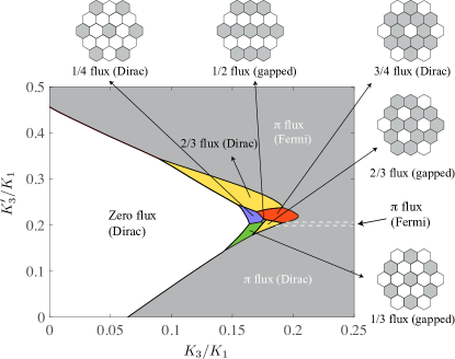
Figure 2: Phase diagram of the extended Kitaev model. Flux configurations of distinct vison crystals (colored phases) are depicted in separate panels; the presence (absence) of a flux is marked at each plaquette by gray (white) filling.

In analogy with how three-spin interactions may be obtained from a Zeeman field Kitaev (2006), the four-spin interactions in Eq. (2) can in principle be generated by a perturbative treatment of Heisenberg and/or symmetric off-diagonal ($\Gamma$) interactions on top of the pure Kitaev model. Taking a more universal approach and considering Eq. (3) as an effective low-energy theory for the Majorana fermions Song et al. (2016), we know that generic time-reversal-symmetric perturbations to ${\cal H}_{K_{1}}$ must generate all Majorana terms that are consistent with the projective symmetries of the Kitaev spin liquid You et al. (2012). Given that all interaction terms are irrelevant and second-neighbor hopping terms are forbidden by time reversal, Eq. (3) is the most natural effective theory beyond the pure Kitaev model.

Phase diagram. The ground state of ${\cal H}_{K_{1}}$ belongs to the zero-flux sector, characterized by $W_{p}=+1$ for all $p$ Kitaev (2006); Lieb (1994). In the presence of the additional interactions, however, the ground state may belong to a wide range of different flux sectors, as shown by the $T=0$ phase diagram in Fig. 2. This phase diagram is obtained from a simple variational analysis, by comparing the energies of the seven flux sectors appearing in the diagram on finite lattices of $48\times 48$ unit cells . Furthermore, it is fully consistent with unbiased finite-temperature MC simulations, discussed in a later section .

We first concentrate on the two fully symmetric non-crystal phases occupying most of the phase diagram: the zero-flux phase, which has no fluxes at any plaquettes, and the $\pi$-flux phase, which has a $\mathbb{Z}_{2}$ flux at each plaquette. For $K_{3}=K_{3}^{\prime}=0$, the creation of each $\mathbb{Z}_{2}$ flux with $W_{p}=-1$ costs a finite energy $\Delta\approx 0.15K_{1}$, and the ground state thus belongs to the zero-flux sector. For $K_{3}/K_{1}>0$, the $K_{1}$ and $K_{3}$ terms in Eq. (3) give rise to a frustrated Majorana hopping and hence an increase in the ground-state energy. However, due to the two paths between any two opposite sites $i$ and $l$ around a plaquette $p$ [see Fig. 1(b)], there are two equivalent hopping terms $\propto iK_{3}c_{i}c_{l}$ in Eq. (3), which interfere constructively for $W_{p}=+1$ and destructively for $W_{p}=-1$. Consequently, as $K_{3}/K_{1}$ is increased, fluxes are effective in relieving frustration from the Majorana hopping and thus become energetically favorable. Since the effective interaction between nearby fluxes is attractive for small $K_{3}^{\prime}/K_{1}$ Kitaev (2006), the corresponding phase transition between the zero-flux and the $\pi$-flux phases is strongly first order.

Increasing $K_{3}^{\prime}/K_{1}$, one can modify this interaction and stabilize various intermediate phases with nontrivial flux configurations. Indeed, there are five distinct translation-symmetry-breaking vison-crystal phases in Fig. 2, with their ordering wave vectors ${\bm{Q}}$ corresponding to either the $\mathrm{K}$ point or the $\mathrm{M}$ point(s) of the Brillouin zone (BZ). The two ${\bm{Q}}={\bm{Q}}_{\mathrm{K}}$ crystals have supercells of three plaquettes, containing one vison (“$1/3$ flux crystal”) and two visons (“$2/3$ flux crystal”), respectively. Since there are three different $\mathrm{M}$ points, ${\bm{Q}}={\bm{Q}}_{\mathrm{M}}$ crystals can exhibit single-${\bm{Q}}$ or multi-${\bm{Q}}$ ordering. The single-${\bm{Q}}$ crystal is a stripy configuration, corresponding to a supercell of two plaquettes containing one vison (“$1/2$ flux crystal”), while the two triple-${\bm{Q}}$ crystals have supercells of four plaquettes, containing one vison (“$1/4$ flux crystal”) and three visons (“$3/4$ flux crystal”), respectively.

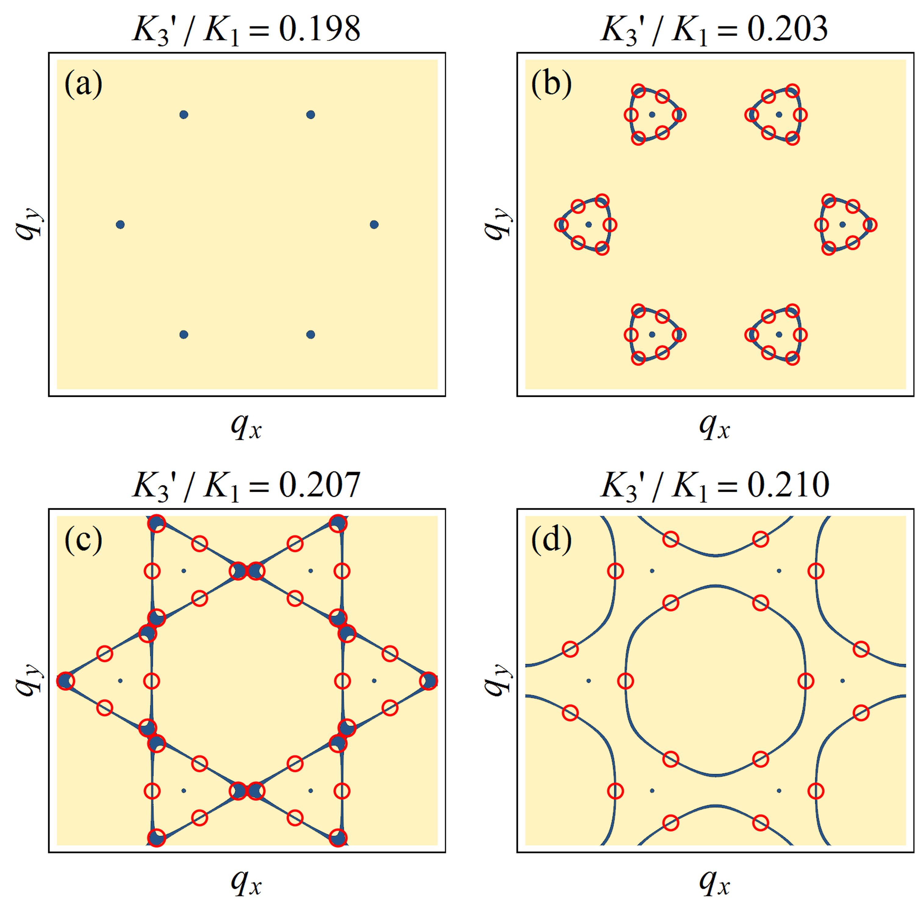
Figure 3: Majorana nodal structures (dark blue) in the various $\pi$-flux phases: the Dirac phase (a), the first Fermi phase (b), the Lifshitz transition between the two Fermi phases (c), and the second Fermi phase (d). In the presence of generic further-neighbor Majorana hopping terms not , each Fermi surface is gapped out into six Dirac points (red circles).

Majorana problems. For the different ground-state flux sectors discussed above, distinct configurations of the gauge fields $u_{ij}^{\alpha}=\pm 1$ lead to different Majorana Hamiltonians in Eq. (3). Consequently, each phase in Fig. 2 has its own Majorana band dispersion and a corresponding density of states. The low-energy physics, giving rise to universal signatures in experiments, is determined by the nodal structures of the Majorana fermions. For the zero-flux phase, including the pure Kitaev model, as well as for the $1/4$ and $3/4$ flux crystals, the Majorana fermions are gapless at Dirac points and thus have linear density of states at low energies. For the $1/3$ and $1/2$ flux crystals, the Majorana fermions are fully gapped and thus have zero density of states below the energy gap. For the $2/3$ flux crystal, there are two disconnected phases where the Majorana fermions are gapless at Dirac points and fully gapped, respectively (see Fig. 2).

Interestingly, the Majorana fermions have more complex nodal structures in the $\pi$-flux phase. This phase is amenable to a full analytic understanding as, due to the perfect cancelation of all $K_{3}$ terms in Eq. (3), the Majorana problem has only one dimensionless parameter ratio $\kappa\equiv K_{3}^{\prime}/K_{1}$. With a simple calculation sup , we find that there are in fact three distinct $\pi$-flux phases characterized by different Majorana nodal structures.

In particular, there is a $\pi$-flux phase where the Majorana fermions are gapless at Dirac points only, and another two $\pi$-flux phases where these Dirac points coexist with Fermi surfaces (i.e., nodal lines) of distinct topologies (see Fig. 3). The dashed lines in Fig. 2 indicate two subsequent Lifshitz transitions Volovik (2003) separating these three phases as a function of increasing $\kappa$. For $\kappa<1/5$, the only nodal structures are Dirac points. At the first Lifshitz transition, $\kappa=1/5$, small pockets of Fermi surfaces appear around these Dirac points and gradually expand as $\kappa$ is further increased. At the second Lifshitz transition, $\kappa=(\sqrt{2}-1)/2\approx 0.207$, these small pockets then connect with each other to form larger pockets. We remark that the Dirac points are located at exactly the same momenta for all values of $\kappa$.

Such a coexistence of Dirac points and Fermi surfaces is rather surprising and is not expected to be stable. Instead, due to the nature of the time-reversal and particle-hole symmetries in the Majorana problem Hermanns and Trebst (2014), one would anticipate only Dirac points to be generically present, as in all the other phases of Fig. 2. Indeed, we find that the Fermi surfaces exist due to the particular simplicity of the problem up to third-neighbor hopping terms sup and that each Fermi surface is gapped out into six Dirac points (see Fig. 3) when generic fifth-neighbor hopping terms not , respecting the projective symmetries of the system, are included in Eq. (3). However, assuming that such terms are small enough, approximate Fermi surfaces are still expected to be observable in experiments.

Experimental signatures. The phase diagram in Fig. 2 contains a rich variety of phases with all possible Majorana nodal structures in two dimensions, including Fermi surfaces, Dirac points, and fully gapped scenarios. Due to their distinct low-energy physics, these phases are characterized by different experimental signatures. First, we expect the low-temperature specific heat to behave as $C\propto T$ for Fermi phases, $C\propto T^{2}$ for Dirac phases, and $C\propto e^{-\Delta_{\text{v}}/T}$ for fully gapped phases, where the activated behavior should be controlled by the vison gap $\Delta_{\text{v}}$ as it is actually smaller than the Majorana gap. Second, the various Majorana nodal structures may be distinguished by their low-energy fingerprints in spectroscopic probes, such as resonant inelastic x-ray scattering Halász et al. (2016, 2017). Third, the Majorana Fermi surface in the $\pi$-flux phase leads to impurity-induced Friedel oscillations in the magnetic energy density sup . In turn, such magnetic Friedel oscillations should be measurable with nuclear magnetic resonance (NMR) as they induce an oscillatory bond-length modulation via magnetostriction.

For the vison-crystal phases in Fig. 2, the spontaneous breaking of translation symmetry leads to further experimental signatures. First of all, due to magnetostriction, each vison crystal generates a characteristic bond-length modulation throughout the lattice, which can be picked up with NMR or elastic x-ray scattering. Moreover, the enlarged unit cell results in a larger number of distinct bands for the Majorana fermions and therefore, in contrast to the pure Kitaev model Knolle et al. (2014, 2015), the dynamical spin structure factor sup , directly measurable by inelastic neutron scattering, has multiple peaks as a function of energy (see Fig. 4). Finally, unlike the fully symmetric phases, each vison-crystal phase has a finite-temperature phase transition at a critical temperature $T_{c}$.

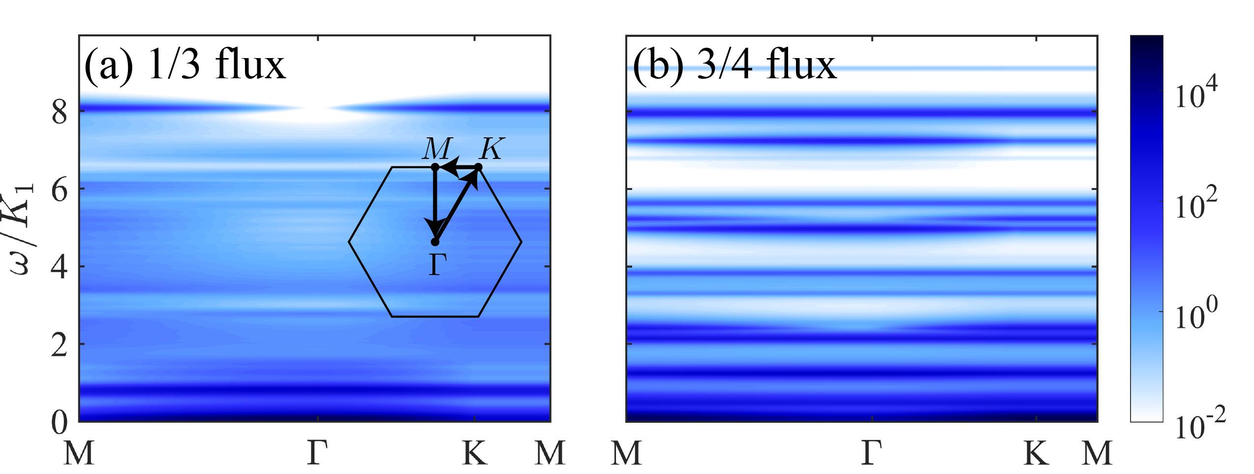
Figure 4: Dynamical spin structure factor $S_{zz}({\bm{q}},\omega)$ sup for the 1/3 flux crystal (a) and the 3/4 flux crystal (b) along the path $\mathrm{M}$-$\Gamma$-$\mathrm{K}$-$\mathrm{M}$ in the Brillouin zone [see inset of panel (a)] via the single-particle approximation of Ref. Knolle et al., 2015.

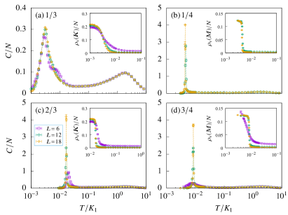
Figure 5: Temperature dependence of the specific heat and the appropriate static vison structure factor for (a) the $1/3$ flux crystal with $K_{3}=0.165K_{1}$ and $K_{3}^{\prime}=0.19K_{1}$, (b) the $1/4$ flux crystal with $K_{3}=0.165K_{1}$ and $K_{3}^{\prime}=0.22K_{1}$, (c) the $2/3$ flux crystal with $K_{3}=0.165K_{1}$ and $K_{3}^{\prime}=0.26K_{1}$, and (d) the $3/4$ flux crystal with $K_{3}=0.19K_{1}$ and $K_{3}^{\prime}=0.22K_{1}$ on $L\times L$ lattices ($L=6,12,18$) containing $N=2L^{2}$ sites.

Monte Carlo simulations. To verify the phase diagram in Fig. 2 and to extract the melting temperatures $T_{c}$ of the vison crystals, we perform MC simulations of ${\cal H}$ based on a Metropolis algorithm to update the “classical” $\mathbb{Z}_{2}$ fields $\{u_{ij}^{\alpha}=\pm 1\}$. The energy of each field configuration is computed by diagonalizing the quadratic Majorana Hamiltonian in Eq. (3) Nasu et al. (2014, 2015) on $L\times L$ lattices with $L=\{6,12,18\}$ sup . For each temperature, a single run contains 10000 MC sweeps for equilibration and another 20000 MC sweeps for measurement .

Figure 5 shows our results for the heat capacity $C(T)$ and the static vison structure factor,

$$\rho_{\text{v}}({\bm{k}})=\frac{1}{L^{2}}\sum_{p,p^{\prime}}e^{i{\bm{k}}\cdot({\bm{X}}_{p}-{\bm{X}}_{p^{\prime}})}\,\langle W_{p}W_{p^{\prime}}\rangle,$$ (4)

for representative parameters of four different vison crystals, where ${\bm{X}}_{p}$ is the position of plaquette $p$, and ${\bm{k}}$ is the ordering wave vector of each vison crystal, corresponding to either the $\mathrm{K}$ or the $\mathrm{M}$ point of the BZ. We first observe that, as for the pure Kitaev model, $C(T)$ exhibits both a high- and a low-temperature peak, which correspond to spinon and vison excitations, respectively (Nasu et al., 2014, 2015). However, the low-temperature peak signals the onset of vison-crystal ordering at $T=T_{c}$, as confirmed by the sharp growth of the corresponding Bragg peak in $\rho_{\text{v}}({\bm{k}})$. While the three lattice sizes $L=\{6,12,18\}$ do not facilitate a rigorous finite-size scaling analysis, the results in Fig. 5 suggest a first-order crystallization transition for all vison crystals, except for the $1/3$ flux crystal . Assuming that the transition into the $1/3$ flux crystal is continuous, it is conjectured to be in the universality class of the two-dimensional $3$-state Potts model, which in turn suggests that the height of the peak in $C(T)/L^{2}$ should be $\propto L^{\alpha/\nu}$ with critical exponents $\alpha=1/3$, $\nu=5/6$, and $\alpha/\nu=2/5$ den Nijs (1979). We note that, for each vison crystal, the critical temperature is $T_{c}\sim 10^{-2}K_{1}$.

Discussion. By considering a natural extension of the honeycomb Kitaev model, we have found a rich spectrum of novel spin-liquid phases that are not adiabatically connected to the original Kitaev model, including a fully symmetric $\pi$-flux spin liquid, and five distinct symmetry-breaking spin liquids with various degrees of vison crystallization. In the future, it would be interesting to study how an external magnetic field affects our spin liquids. For the Dirac phases, it may generate non-Abelian gapped spin liquids with distinct Chern numbers of the Majorana fermions Kitaev (2006). For the gapped phases, it may lead to nontrivial finite-field phase transitions between topologically distinct spin liquids.

We thank Arnab Banerjee, Hiroaki Ishizuka, and Johannes Knolle for useful comments on the manuscript. S.-S.Z., Z.W., and C.D.B. are supported by funding from the Lincoln Chair of Excellence in Physics. The work of G.B.H. at ORNL was supported by Laboratory Director’s Research and Development funds. This research used resources of the Oak Ridge Leadership Computing Facility, which is a DOE Office of Science User Facility supported under Contract DE-AC05-00OR22725.

.1 Supplemental Material

I Derivation of the Majorana Hamiltonian

The spin Hamiltonian $\mathcal{H}$ in Eq. (1) of the main text is exactly solvable by means of a standard procedure described in Ref. 1 of the main text. The first step is to introduce four Majorana fermions $b_{j}^{x}$, $b_{j}^{y}$, $b_{j}^{z}$, and $c_{j}^{\phantom{{\dagger}}}$ at each site $j$ of the honeycomb lattice, and express the spin components $\sigma_{j}^{x,y,z}$ in terms of these Majorana fermions as

$$\sigma_{j}^{x}=ib_{j}^{x}c_{j}^{\phantom{{\dagger}}},\qquad\sigma_{j}^{y}=ib_{j}^{y}c_{j}^{\phantom{{\dagger}}},\qquad\sigma_{j}^{z}=ib_{j}^{z}c_{j}^{\phantom{{\dagger}}}.$$ (S1)

Due to the resulting enlargement of the local Hilbert space, the four Majorana fermions must be reconciled with the original spin degree of freedom via the local gauge constraint

$${-}i\sigma_{j}^{x}\sigma_{j}^{y}\sigma_{j}^{z}=b_{j}^{x}b_{j}^{y}b_{j}^{z}c_{j}^{\phantom{{\dagger}}}=1.$$ (S2)

In turn, the corresponding gauge redundancy means that the expressions in Eq. (S1) for the spin components are not unique; for example, one can use Eq. (S2) to obtain the following equivalent expressions:

$$\sigma_{j}^{x}=-ib_{j}^{y}b_{j}^{z},\qquad\sigma_{j}^{y}=-ib_{j}^{z}b_{j}^{x},\qquad\sigma_{j}^{z}=-ib_{j}^{x}b_{j}^{y}.$$ (S3)

Employing Eqs. (S1) and/or (S3) appropriately, the two terms ${\cal H}_{K_{1}}$ and ${\cal H}_{K_{3}}$ of the spin Hamiltonian $\mathcal{H}$ then become

$${\cal H}_{K_{1}} = -K_{1}\sum_{\langle ij\rangle_{\alpha}}\sigma^{\alpha}_{i}\sigma^{\alpha}_{j}=-K_{1}\sum_{\langle ij\rangle_{\alpha}}\big{(}ib_{i}^{\alpha}c_{i}^{\phantom{{\dagger}}}\big{)}\big{(}ib_{j}^{\alpha}c_{j}^{\phantom{{\dagger}}}\big{)}=iK_{1}\sum_{\langle ij\rangle_{\alpha}}\big{(}ib_{i}^{\alpha}b_{j}^{\alpha}\big{)}\,c_{i}^{\phantom{{\dagger}}}c_{j}^{\phantom{{\dagger}}},$$

$${\cal H}_{K_{3}} = K_{3}\sum_{\langle ijkl\rangle_{\alpha\beta\gamma}}\sigma_{i}^{\alpha}\sigma_{j}^{\gamma}\sigma_{k}^{\alpha}\sigma_{l}^{\gamma}-K_{3}^{\prime}\sum_{\langle ijkl\rangle_{\alpha\beta\alpha}}\sigma_{i}^{\alpha}\sigma_{j}^{\gamma}\sigma_{k}^{\gamma}\sigma_{l}^{\alpha}$$

$$= K_{3}\sum_{\langle ijkl\rangle_{\alpha\beta\gamma}}\big{(}ib_{i}^{\alpha}c_{i}^{\phantom{{\dagger}}}\big{)}\big{(}{-}ib_{j}^{\alpha}b_{j}^{\beta}\big{)}\big{(}{-}ib_{k}^{\beta}b_{k}^{\gamma}\big{)}\big{(}ib_{l}^{\gamma}c_{l}^{\phantom{{\dagger}}}\big{)}-K_{3}^{\prime}\sum_{\langle ijkl\rangle_{\alpha\beta\alpha}}\big{(}ib_{i}^{\alpha}c_{i}^{\phantom{{\dagger}}}\big{)}\big{(}{-}ib_{j}^{\alpha}b_{j}^{\beta}\big{)}\big{(}{-}ib_{k}^{\alpha}b_{k}^{\beta}\big{)}\big{(}ib_{l}^{\alpha}c_{l}^{\phantom{{\dagger}}}\big{)}$$

$$= iK_{3}\sum_{\langle ijkl\rangle_{\alpha\beta\gamma}}\big{(}ib_{i}^{\alpha}b_{j}^{\alpha}\big{)}\big{(}ib_{k}^{\beta}b_{j}^{\beta}\big{)}\big{(}ib_{k}^{\gamma}b_{l}^{\gamma}\big{)}\,c_{i}^{\phantom{{\dagger}}}c_{l}^{\phantom{{\dagger}}}+iK_{3}^{\prime}\sum_{\langle ijkl\rangle_{\alpha\beta\alpha}}\big{(}ib_{i}^{\alpha}b_{j}^{\alpha}\big{)}\big{(}ib_{k}^{\beta}b_{j}^{\beta}\big{)}\big{(}ib_{k}^{\alpha}b_{l}^{\alpha}\big{)}\,c_{i}^{\phantom{{\dagger}}}c_{l}^{\phantom{{\dagger}}}.$$

Substituting Eq. (I) into Eq. (1) of the main text, and introducing the $\mathbb{Z}_{2}$ gauge fields $u_{ij}^{\alpha}\equiv ib_{i}^{\alpha}b_{j}^{\alpha}$, one immediately recovers the Majorana Hamiltonian in Eq. (3) of the main text. Since the $\mathbb{Z}_{2}$ gauge fields are mutually commuting conserved quantities, $u_{ij}^{\alpha}=\pm 1$, this Majorana Hamiltonian is quadratic and hence exactly solvable.

II Quadratic Majorana problems

For each phase in Fig. 2 of the main text, the ground-state flux configuration can be represented with an appropriate gauge configuration $u_{ij}^{\alpha}=\pm 1$ (see Fig. S1). For all phases other than the zero-flux phase, the effective unit cell of the Majorana fermions is enlarged with respect to the honeycomb unit cell as a result of physical symmetry breaking (flux crystallization) and/or ostensible symmetry breaking (gauge freedom in representing each $\pi$ flux). We label each site of the honeycomb lattice as $i\equiv(\Theta,{\bm{R}},\lambda)$, where $\Theta=\{A,B\}$ is a sublattice index, ${\bm{R}}$ is the lattice vector of the enlarged unit cell, and $\lambda=1,\dots,n$ specifies the particular honeycomb unit cell within the enlarged unit cell. Note that $n=1$ for the zero-flux phase, $n=2$ for the $\pi$-flux phase, and $n>2$ for the flux-crystal phases.

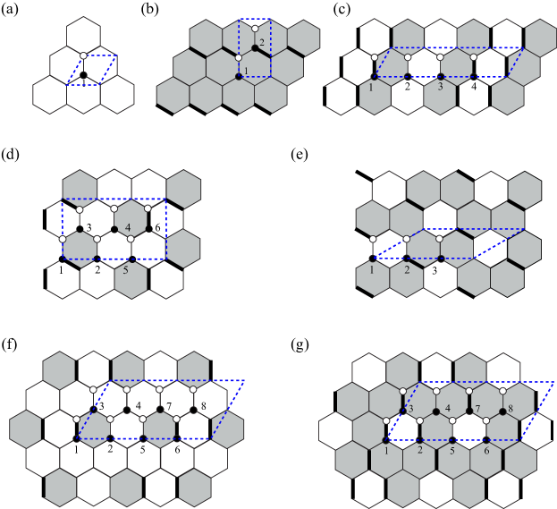
Figure S1: Gauge representation of the flux configuration for the zero-flux phase (a), the $\pi$-flux phase (b), the $1/2$ flux crystal (c), the $1/3$ flux crystal (d), the $2/3$ flux crystal (e), the $1/4$ flux crystal (f), and the $3/4$ flux crystal (g). In each case, bonds with $u_{ij}^{\alpha}=-1$ are denoted by thick lines. Note that the effective unit cell (blue dashed parallelogram) may contain several honeycomb unit cells, labeled by $\lambda=1,\dots,n$, each containing one $A$ site (black dot) and one $B$ site (white dot).

Using this notation, the quadratic Majorana Hamiltonian in Eq. (3) of the main text takes the general form

$$\mathcal{H}=\sum_{{\bm{R}},{\bm{R}}^{\prime}}\sum_{\lambda,\lambda^{\prime}}i\mathcal{M}_{{\bm{R}}^{\prime}-{\bm{R}},\lambda,\lambda^{\prime}}^{\phantom{{\dagger}}}\,c_{A,{\bm{R}},\lambda}^{\phantom{{\dagger}}}\,c_{B,{\bm{R}}^{\prime},\lambda^{\prime}}^{\phantom{{\dagger}}},$$ (S5)

where each $\mathcal{M}_{{\bm{R}}^{\prime}-{\bm{R}},\lambda,\lambda^{\prime}}$ is a product of gauge fields $u_{ij}^{\alpha}=\pm 1$ along a path connecting the sites $(A,{\bm{R}},\lambda)$ and $(B,{\bm{R}}^{\prime},\lambda^{\prime})$ occupied by the Majorana fermions $c_{A,{\bm{R}},\lambda}^{\phantom{{\dagger}}}$ and $c_{B,{\bm{R}}^{\prime},\lambda^{\prime}}^{\phantom{{\dagger}}}$. In terms of the momentum-space complex fermions

$$\psi_{A(B),{\bm{q}},\lambda}^{\phantom{{\dagger}}}=\frac{1}{\sqrt{N}}\sum_{{\bm{R}}}c_{A(B),{\bm{R}},\lambda}^{\phantom{{\dagger}}}\,e^{-i{\bm{q}}\cdot{\bm{R}}},\qquad\psi_{A(B),{\bm{q}},\lambda}^{{\dagger}}=\psi_{A(B),-{\bm{q}},\lambda}^{\phantom{{\dagger}}}=\frac{1}{\sqrt{N}}\sum_{{\bm{R}}}c_{A(B),{\bm{R}},\lambda}^{\phantom{{\dagger}}}\,e^{i{\bm{q}}\cdot{\bm{R}}},$$ (S6)

where $N$ is the number of sites, the Hamiltonian in Eq. (S5) assumes the standard Bogoliubov–de Gennes form

$$\mathcal{H}=2\sum_{\pm{\bm{q}}}\sum_{\lambda,\lambda^{\prime}}\left(i\hat{\mathcal{M}}_{{\bm{q}},\lambda,\lambda^{\prime}}^{\phantom{*}}\,\psi_{A,{\bm{q}},\lambda}^{{\dagger}}\,\psi_{B,{\bm{q}},\lambda^{\prime}}^{\phantom{{\dagger}}}+i\hat{\mathcal{M}}_{{\bm{q}},\lambda,\lambda^{\prime}}^{*}\,\psi_{A,{\bm{q}},\lambda}^{\phantom{{\dagger}}}\,\psi_{B,{\bm{q}},\lambda^{\prime}}^{{\dagger}}\right)=2\sum_{\pm{\bm{q}}}\left(\begin{array}[]{cc}\psi_{A,{\bm{q}}}^{{\dagger}}&\psi_{B,{\bm{q}}}^{{\dagger}}\end{array}\right)\left(\begin{array}[]{cc}0&i\hat{\mathcal{M}}_{{\bm{q}}}^{\phantom{{\dagger}}}\\ -i\hat{\mathcal{M}}_{{\bm{q}}}^{{\dagger}}&0\end{array}\right)\left(\begin{array}[]{c}\psi_{A,{\bm{q}}}^{\phantom{{\dagger}}}\\ \psi_{B,{\bm{q}}}^{\phantom{{\dagger}}}\end{array}\right),$$ (S12)

$$\qquad\qquad\hat{\mathcal{M}}_{{\bm{q}},\lambda,\lambda^{\prime}}^{\phantom{{\dagger}}}=\sum_{{\bm{r}}}\mathcal{M}_{{\bm{r}},\lambda,\lambda^{\prime}}^{\phantom{{\dagger}}}\,e^{i{\bm{q}}\cdot{\bm{r}}},\qquad\qquad\psi_{A(B),{\bm{q}}}^{\phantom{{\dagger}}}\equiv\left(\psi_{A(B),{\bm{q}},1}^{\phantom{{\dagger}}},\dots,\psi_{A(B),{\bm{q}},n}^{\phantom{{\dagger}}}\right)^{T},$$ (S13)

where the summation is over pairs of momenta $\pm{\bm{q}}$ due to the particle-hole redundancy $\psi_{A(B),{\bm{q}}}^{\phantom{{\dagger}}}=\psi_{A(B),-{\bm{q}}}^{{\dagger}}$. Using the particular structure of this quadratic Hamiltonian, reflecting time-reversal symmetry, the Majorana energies at each momentum $\pm{\bm{q}}$ are then given by the singular values of the $n\times n$ matrix $\hat{\mathcal{M}}_{{\bm{q}}}^{\phantom{{\dagger}}}$.

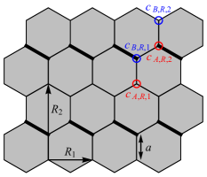
Figure S2: Labeling convention for the $\pi$-flux phase, including the lattice constant $a$, the lattice vectors ${\bm{R}}_{1,2}$, and the four sites within each unit cell. The gauge configuration is also specified; bonds with $u_{ij}^{\alpha}=-1$ are denoted by thick lines.

III Majorana nodal structures

From Eq. (S13), the nodal structures of the Majorana fermions are characterized by vanishing singular values of $\hat{\mathcal{M}}_{{\bm{q}}}^{\phantom{{\dagger}}}$ or, equivalently, by $\det\hat{\mathcal{M}}_{{\bm{q}}}^{\phantom{{\dagger}}}=0$. Since $\det\hat{\mathcal{M}}_{{\bm{q}}}^{\phantom{{\dagger}}}$ is generically complex, $\det\hat{\mathcal{M}}_{{\bm{q}}}^{\phantom{{\dagger}}}=0$ translates into two independent equations for its real and imaginary parts. Consequently, for each phase in Fig. 2 of the main text, any nodal structures are anticipated to be of codimension $2$, corresponding to point nodes in two dimensions. Indeed, we generically find that the Majorana fermions are either fully gapped or gapless at discrete points only.

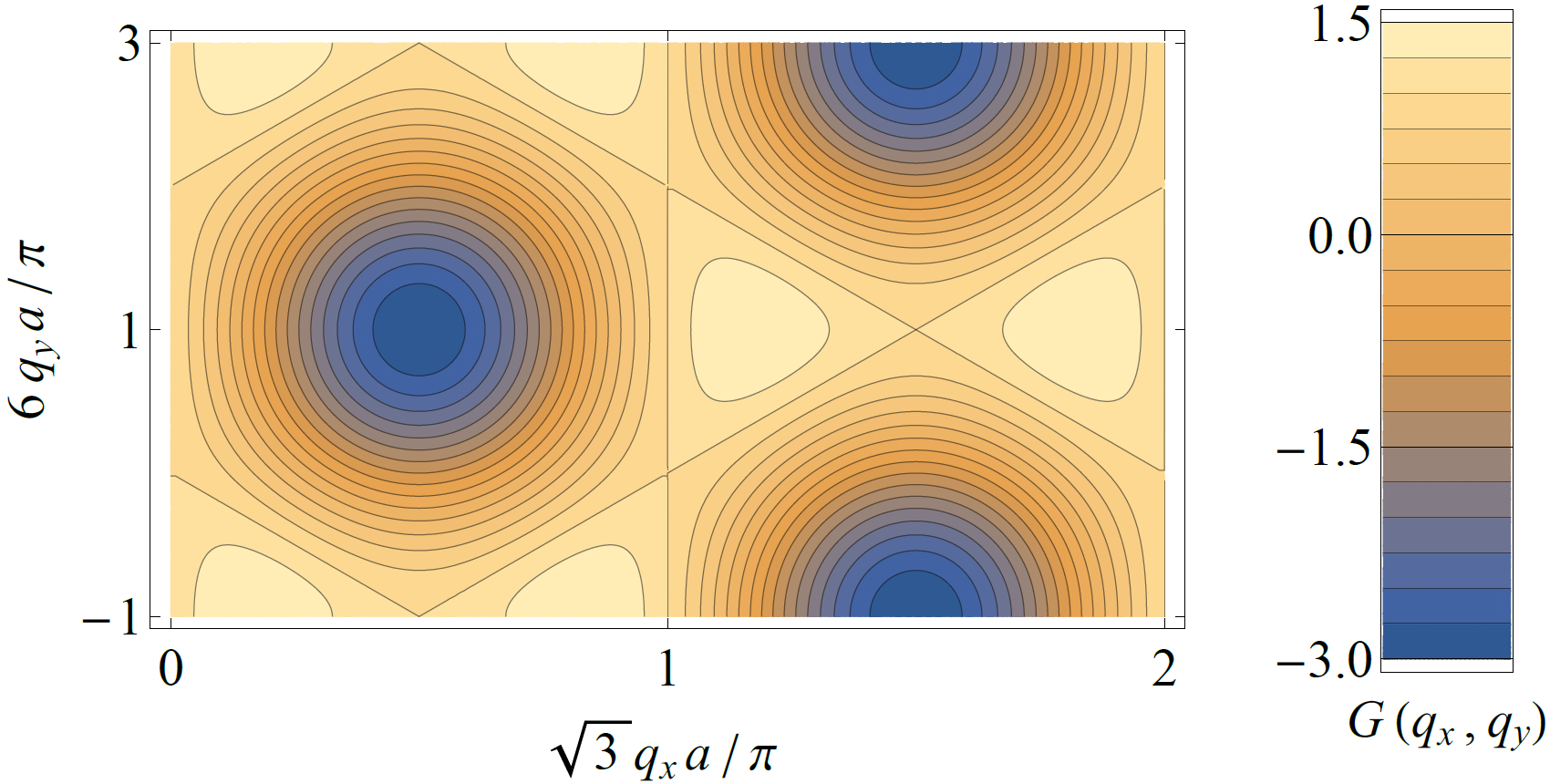
Figure S3: Contour plot of the function $G({\bm{q}})$ as a function of the momentum components $q_{x}$ and $q_{y}$.

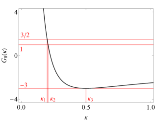
Figure S4: Plot of the function $G_{0}(\kappa)$ as a function of the dimensionless parameter $\kappa=K_{3}^{\prime}/K_{1}$.

However, for the $\pi$-flux phase, if we only consider first-neighbor and third-neighbor Majorana hopping with amplitudes $K_{1}$ and $K_{3}^{\prime}$, respectively, the Majorana problem takes a particularly simple form. Using the labeling convention in Fig. S2, the matrix elements of the $2\times 2$ matrix $\hat{\mathcal{M}}_{{\bm{q}}}^{\phantom{{\dagger}}}$ in Eq. (S13) are given by

$$\hat{\mathcal{M}}_{{\bm{q}},1,1}^{\phantom{{\dagger}}}=\hat{\mathcal{M}}_{{\bm{q}},2,2}^{\phantom{{\dagger}}}=K_{1}+K_{3}^{\prime}e^{-i{\bm{q}}\cdot({\bm{R}}_{1}+{\bm{R}}_{2})}-K_{3}^{\prime}e^{i{\bm{q}}\cdot({\bm{R}}_{1}-{\bm{R}}_{2})},$$

$$\hat{\mathcal{M}}_{{\bm{q}},1,2}^{\phantom{{\dagger}}}=K_{1}e^{-i{\bm{q}}\cdot({\bm{R}}_{1}+{\bm{R}}_{2})}+K_{1}e^{-i{\bm{q}}\cdot{\bm{R}}_{2}}+K_{3}^{\prime}e^{-i{\bm{q}}\cdot(2{\bm{R}}_{1}+{\bm{R}}_{2})}-K_{3}^{\prime}e^{-i{\bm{q}}\cdot{\bm{R}}_{1}}+K_{3}^{\prime}+K_{3}^{\prime}e^{i{\bm{q}}\cdot({\bm{R}}_{1}-{\bm{R}}_{2})},\qquad$$ (S14)

$$\hat{\mathcal{M}}_{{\bm{q}},2,1}^{\phantom{{\dagger}}}=K_{1}-K_{1}e^{i{\bm{q}}\cdot{\bm{R}}_{1}}-K_{3}^{\prime}e^{-i{\bm{q}}\cdot{\bm{R}}_{1}}+K_{3}^{\prime}e^{i{\bm{q}}\cdot{\bm{R}}_{2}}+K_{3}^{\prime}e^{i{\bm{q}}\cdot({\bm{R}}_{1}+{\bm{R}}_{2})}+K_{3}^{\prime}e^{2i{\bm{q}}\cdot{\bm{R}}_{1}},$$

and the determinant of $\hat{\mathcal{M}}_{{\bm{q}}}^{\phantom{{\dagger}}}$ readily factorizes into the product form

$$\det\hat{\mathcal{M}}_{{\bm{q}}}^{\phantom{{\dagger}}}=K_{1}^{2}F({\bm{q}})\left[1-2\kappa(2+\kappa)-2\kappa^{2}G({\bm{q}})\right],$$ (S15)

where $\kappa\equiv K_{3}^{\prime}/K_{1}$ is the dimensionless third-neighbor hopping amplitude, and the two functions $F({\bm{q}})$ and $G({\bm{q}})$ are

$$F({\bm{q}}) = 1+2ie^{-3iq_{y}a}\sin\left(\sqrt{3}q_{x}a\right),$$

$$G({\bm{q}}) = \cos\left(2\sqrt{3}q_{x}a\right)-2\sin\left(2\sqrt{3}q_{x}a\right)\sin\left(3q_{y}a\right).$$ (S16)

While the function $F({\bm{q}})$ is complex, and the solutions of $F({\bm{q}})=0$ thus give point nodes at $q_{x}a=\pm\pi/(6\sqrt{3})+2\pi n_{x}/\sqrt{3}$ and $q_{y}a=\mp\pi/6+2\pi n_{y}/3$ as well as at $q_{x}a=\pm 5\pi/(6\sqrt{3})+2\pi n_{x}/\sqrt{3}$ and $q_{y}a=\mp\pi/6+2\pi n_{y}/3$ (with $n_{x},n_{y}\in\mathbb{Z}$), the function $G({\bm{q}})$ plotted in Fig. S3 is real, with a minimum value $G_{\mathrm{min}}=-3$, a maximum value $G_{\mathrm{max}}=3/2$, and a critical value $G_{\mathrm{vH}}=1$ corresponding to a van Hove singularity. Consequently, the solutions of $1-2\kappa(2+\kappa)-2\kappa^{2}G({\bm{q}})=0$ generically correspond to nodal lines along the contours of Fig. S3 given by

$$G({\bm{q}})=G_{0}(\kappa)\equiv\frac{1-2\kappa(2+\kappa)}{2\kappa^{2}}\,.$$ (S17)

To analyze these nodal lines, we plot $G_{0}(\kappa)$ in Fig. S4 and find three critical values of $\kappa$ between $0$ and $1$:

$$\kappa_{1}=0.2,\qquad\kappa_{2}=\frac{1}{2}\big{(}\sqrt{2}-1\big{)}\approx 0.207,\qquad\kappa_{3}=0.5.$$ (S18)

For $\kappa<\kappa_{1}$, we obtain $G_{0}(\kappa)>G_{\mathrm{max}}$, and Eq. (S17) has no solutions. For $\kappa_{1}<\kappa<\kappa_{2}$, we obtain $G_{\mathrm{vH}}<G_{0}(\kappa)<G_{\mathrm{max}}$, and the solutions of Eq. (S17) are nodal lines surrounding the maxima of $G({\bm{q}})$. Interestingly, these maxima coincide with the point nodes characterized by $F({\bm{q}})=0$. Finally, for $\kappa>\kappa_{2}$, we obtain $G_{\mathrm{min}}\leq G_{0}(\kappa)<G_{\mathrm{vH}}$, and the solutions of Eq. (S17) are nodal lines surrounding the minima of $G({\bm{q}})$. In particular, for $\kappa=\kappa_{3}$, these nodal lines contract to point nodes as $G_{0}(\kappa)=G_{\mathrm{min}}$.

IV Magnetic Friedel oscillations

In principle, a non-magnetic impurity, such as a spin vacancy [see Fig. S5(a)], can be used as a “physical probe” to distinguish between the $\pi$-flux phases with Dirac points and Fermi surfaces of Majorana fermions. Such an impurity induces a local modulation of the bond energy $E_{\langle ij\rangle_{\alpha}}\propto\langle\sigma_{i}^{\alpha}\sigma_{j}^{\alpha}\rangle$, which decays with a power law as a function of distance; Friedel oscillations are expected to be present (absent) in this decay if the Majorana fermions are gapless at Fermi surfaces (Dirac points). We therefore calculate the radial Fourier transform of the bond-energy modulation,

$$\Delta E(p)=\frac{1}{N}\sum_{\langle ij\rangle_{\alpha}}e^{-ipr_{\langle ij\rangle_{\alpha}}}\left[E_{\langle ij\rangle_{\alpha}}^{\phantom{(0)}}-E_{\langle ij\rangle_{\alpha}}^{(0)}\right],$$ (S19)

in both phases [see Fig. S5(b)], where $r_{\langle ij\rangle_{\alpha}}$ is the distance of the bond $\langle ij\rangle_{\alpha}$ from the impurity, and $E_{\langle ij\rangle_{\alpha}}^{(0)}$ is the bond energy in the absence of the impurity. As expected, in the Dirac phase, $\Delta E(p)$ is peaked at $p=0$, while in the Fermi phase, its peak is shifted to $p\approx 2q_{F}$, where $q_{F}$ is the radius of the Fermi surface [see Fig. S5(c)].

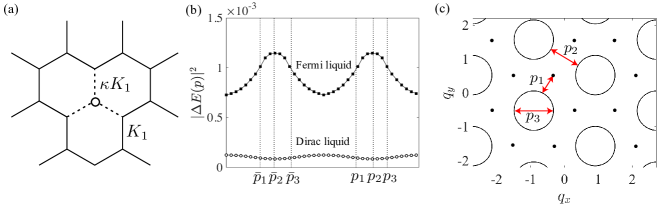
Figure S5: (a) Local distortion of the Kitaev interactions ($\kappa\neq 1$) around a nonmagnetic impurity; the particular case of a spin vacancy corresponds to $\kappa=0$. (b) Radial Fourier transform of the bond-energy modulation around the impurity for the $\pi$-flux phases with Dirac nodes (white circles) and Fermi surfaces (black squares) of Majorana fermions. (c) For the Fermi phase, the peak wave vector of Friedel oscillations is compared with the characteristic dimensions of the Fermi surfaces.

V Dynamical spin structure factor

The dynamical spin structure factor $S_{\mu\nu}({\bm{q}},\omega)$ is probed experimentally by inelastic neutron scattering. At $T=0$, it is given by the spatial and temporal Fourier transform of the spin-spin correlation function in the ground state:

$$S_{\mu\nu}({\bm{q}},\omega)=\frac{1}{2\pi N}\sum_{i,j}\int_{-\infty}^{+\infty}dt\,e^{i\omega t-i{\bm{q}}\cdot({\bm{r}}_{j}-{\bm{r}}_{i})}\,\big{\langle}\sigma_{i}^{\mu}(t)\sigma_{j}^{\nu}(0)\big{\rangle},$$ (S20)

where $\sigma_{i}^{\mu}(t)\equiv e^{i\mathcal{H}t}\sigma_{i}^{\mu}e^{-i\mathcal{H}t}$, and ${\bm{r}}_{i}$ is the position of site $i$. For the general Hamiltonian $\mathcal{H}$ in Eq. (1) of the main text, the spin-spin correlation function $\langle\sigma_{i}^{\mu}(t)\sigma_{j}^{\nu}(0)\rangle$ vanishes unless $\mu=\nu$. Moreover, its has an extremely limited range: $\langle\sigma_{i}^{\mu}(t)\sigma_{j}^{\mu}(0)\rangle$ is only nonzero if $i$ and $j$ are the same site ($i=j$) or if they are nearest-neighbor sites connected by a $\mu$ bond $\langle ij\rangle_{\mu}$. The structure factor in Eq. (S20) is thus generally given by

$$S_{\mu\nu}({\bm{q}},\omega)=\delta_{\mu\nu}\left[S_{\mu\mu}^{(0)}(\omega)+2\cos({\bm{q}}\cdot{\bm{n}}_{\mu})\,S_{\mu\mu}^{(1)}(\omega)\right],$$ (S21)

where $S_{\mu\mu}^{(0)}(\omega)$ and $S_{\mu\mu}^{(1)}(\omega)$ are on-site and nearest-neighbor contributions,

$$S_{\mu\mu}^{(0)}(\omega)=\frac{1}{N}\sum_{i}S_{\mu\mu,i}^{(0)}(\omega),\qquad\qquad S_{\mu\mu,i}^{(0)}(\omega)=\frac{1}{2\pi}\int_{-\infty}^{+\infty}dt\,e^{i\omega t}\,\big{\langle}\sigma_{i}^{\mu}(t)\sigma_{i}^{\mu}(0)\big{\rangle},$$ (S22)

$$S_{\mu\mu}^{(1)}(\omega)=\frac{1}{N}\sum_{\langle ij\rangle_{\mu}}S_{\mu\mu,\langle ij\rangle_{\mu}}^{(1)}(\omega),\qquad\,S_{\mu\mu,\langle ij\rangle_{\mu}}^{(1)}(\omega)=\frac{1}{2\pi}\int_{-\infty}^{+\infty}dt\,e^{i\omega t}\,\big{\langle}\sigma_{i}^{\mu}(t)\sigma_{j}^{\mu}(0)\big{\rangle},$$

and ${\bm{n}}_{\mu}$ is the vector connecting the two sites $i$ and $j$ along any $\mu$ bond $\langle ij\rangle_{\mu}$. Note that $\langle\sigma_{i}^{\mu}(t)\sigma_{j}^{\mu}(0)\rangle=\langle\sigma_{j}^{\mu}(t)\sigma_{i}^{\mu}(0)\rangle$ and, consequently, $S_{\mu\mu,\langle ij\rangle_{\mu}}^{(1)}(\omega)$ is real due to time-reversal symmetry.

The general results in Eqs. (S21) and (S22) are simplified by the unbroken space-group symmetries in each phase of Fig. 2 in the main text. First of all, due to translation symmetry, there are only a finite number of inequivalent sites $i$ and inequivalent $\mu$ bonds $\langle ij\rangle_{\mu}$, and the infinite averages in Eq. (S22) can thus be substituted with finite averages over the $n_{(0)}$ inequivalent sites and the $n_{(1)}$ inequivalent $\mu$ bonds. In particular, $n_{(0)}=n_{(1)}=1$ for each symmetric phase, while $n_{(0)}=n_{(1)}=r$ for each flux crystal with a supercell of $r$ plaquettes. Moreover, for all phases other than the $1/2$ flux crystal, there is a threefold rotation symmetry around the center of some plaquette, which permutes the spin components as $z\rightarrow x\rightarrow y\rightarrow z$ and therefore implies $S_{xx}^{(0,1)}(\omega)=S_{yy}^{(0,1)}(\omega)=S_{zz}^{(0,1)}(\omega)$. For the $1/2$ flux crystal, this rotation symmetry is spontaneously broken; if the flux stripes are perpendicular to the $y$ bonds, as in Fig. S1(c), the remaining point-group symmetries still imply $S_{xx}^{(0,1)}(\omega)=S_{zz}^{(0,1)}(\omega)$.

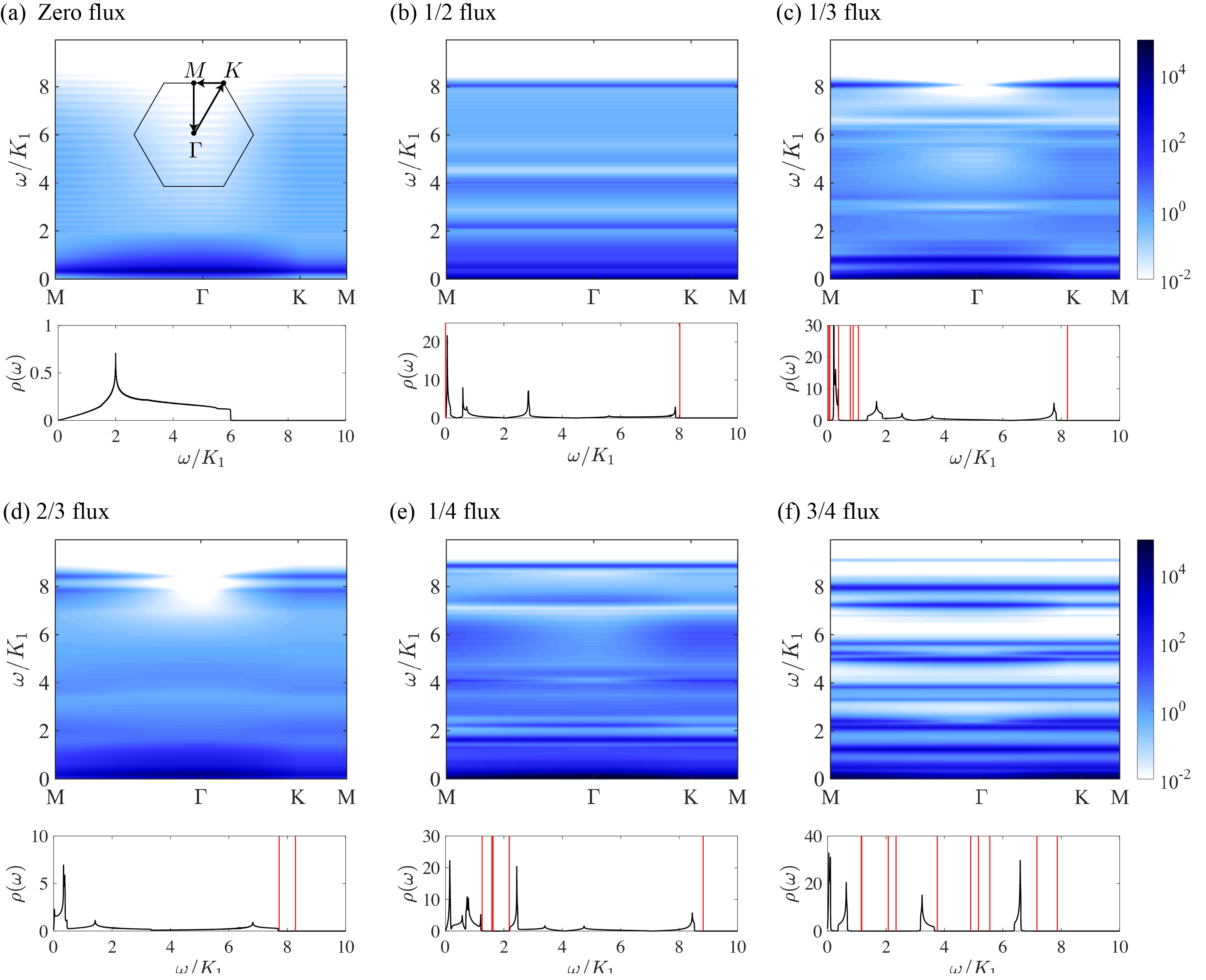
Figure S6: Upper panel of (a)-(f): Dynamical spin structure factor $S_{zz}({\bm{q}},\omega)$ at $T=0$ along the path $\mathrm{M}$-$\Gamma$-$\mathrm{K}$-$\mathrm{M}$ [see inset of (a)] for various phases in Fig. 2 of the main text. Each response is convolved, as a function of energy, with a Lorentzian broadening function of width $\eta=0.05K_{1}$. Lower panel of (a)-(f): Majorana density of states $\rho(\omega)$ for each phase. Red vertical lines are $\delta$ peaks corresponding to additional localized states that appear in the intermediate flux sector of the Lehmann representation.

In Fig. S6, we present the dynamical spin structure factor $S_{zz}({\bm{q}},\omega)$ at $T=0$ for each flux-crystal phase along the high-symmetry path $\mathrm{M}$-$\Gamma$-$\mathrm{K}$-$\mathrm{M}$ in the Brillouin zone [see inset of panel (a)]. Following the few-particle approach in Ref. Knolle et al., 2015, we take the Lehmann representation of $S_{zz}(\bm{q},\omega)$ and restrict our attention to intermediate states containing a single Majorana excitation. If this approximation is valid, the calculated response should approximately satisfy the sum rule $\int d\omega\,S_{zz}^{(0)}(\omega)=1$; for all of the results in Fig. S6, we find that $\int d\omega\,S_{zz}^{(0)}(\omega)>0.6$.

The energy dependence of the dynamical spin structure factor reflects the Majorana density of states in the intermediate flux sector of the Lehmann representation (see Fig. S6). Due to the two fluxes created (or destroyed) by the spin operator $\sigma_{l}^{z}$, the Majorana fermions in the intermediate flux sector are perturbed with respect to the ground-state flux sector, and they may even form localized states around the site $l$. Such a localized state corresponds to a delta peak in the density of states and thus gives rise to a sharp feature in $S_{zz}({\bm{q}},\omega)$. Physically, it can be understood as a magnon bound state, $\sigma_{l}^{z}=ib_{l}^{z}c_{l}^{\phantom{{\dagger}}}$, of a bond Majorana fermion $b_{l}^{z}$ and a matter Majorana fermion $c_{l}^{\phantom{{\dagger}}}$.

VI Monte Carlo implementation

The Monte Carlo (MC) simulations are implemented on an $L\times L$ honeycomb lattice with dimensions $\bm{L}_{1}=L\bm{a}_{1}$ and $\bm{L}_{2}=L\bm{a}_{2}$ and periodic boundary conditions (PBC) in both directions (see Fig. S7). However, using these boundary conditions, a naive numerical implementation would be extremely tedious, and we therefore simplify the procedure by removing a single bond from the lattice.

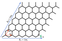
Figure S7: Honeycomb lattice for the Monte Carlo simulations. We employ periodic boundary conditions in both directions but remove a single $y$ bond (marked by the cross) to avoid a tedious numerical procedure.

Indeed, since the Hilbert space is enlarged by the introduction of the Majorana fermions, any state in the Majorana representation must be projected back into the physical Hilbert space. Due to this projection, distinct states in the Majorana representation may correspond to the same physical state, and certain states in the Majorana representation may not correspond to any physical state at all. In fact, each physical state can be represented by $2^{N-1}$ distinct Majorana states, and the total fermion number, $N_{b}+N_{c}$, including bond and matter fermions, is even for all of them:

$$(-1)^{N_{b}}(-1)^{N_{c}}=\Bigg{[}\prod_{\langle jk\rangle_{\alpha}}u_{jk}^{\alpha}\Bigg{]}\Bigg{[}\prod_{\langle jk\rangle_{z}}w_{jk}\Bigg{]}=+1,$$ (S23)

where $u_{jk}^{\alpha}\equiv ib_{j}^{\alpha}b_{k}^{\alpha}$ (as in the main text) and $w_{jk}\equiv ic_{j}c_{k}$. The remaining Majorana states with odd fermion number do not correspond to any physical state as they are annihilated by the projection. The partition function is then

$$Z=\frac{1}{2^{N-1}}\,\text{Tr}_{\{u_{jk}^{\alpha}\}_{\text{even}}}\text{Tr}_{\{w_{jk}\}_{\text{even}}}e^{-\beta\mathcal{H}}+\frac{1}{2^{N-1}}\,\text{Tr}_{\{u_{jk}^{\alpha}\}_{\text{odd}}}\text{Tr}_{\{w_{jk}\}_{\text{odd}}}e^{-\beta\mathcal{H}},$$ (S24)

where $\text{Tr}_{\{u_{jk}^{\alpha}\}_{\text{even}}}$ ($\text{Tr}_{\{u_{jk}^{\alpha}\}_{\text{odd}}}$) sums over all bond-fermion configurations $\{u_{jk}^{\alpha}\}$ with $\prod_{\langle jk\rangle_{\alpha}}u_{jk}^{\alpha}=+1$ ($-1$), while $\text{Tr}_{\{w_{jk}\}_{\text{even}}}$ ($\text{Tr}_{\{w_{jk}\}_{\text{odd}}}$) sums over all matter-fermion configurations $\{w_{jk}\}$ with $\prod_{\langle jk\rangle_{z}}w_{jk}=+1$ ($-1$).

For the relatively small system sizes accessible with MC, it is important to take proper care of the even/odd projections, which in turn makes the MC implementation extremely tedious. However, the computation is simplified tremendously if we remove a single bond $\langle gh\rangle_{y}$ from the lattice (see Fig. S7) by switching off all interactions that involve both sites $g$ and $h$ Nasu et al. (2014). In this case, the Hamiltonian $\mathcal{H}$ does not depend on $u_{gh}^{y}$ and, by switching between $u_{gh}^{y}=\pm 1$, one can switch the bond-fermion parity $\prod_{\langle jk\rangle_{\alpha}}u_{jk}^{\alpha}$ without affecting the spectrum of the matter fermions at all. The partition function in Eq. (S24) can then be written as

$$Z=\frac{1}{2^{N-1}}\,\text{Tr}_{\{u_{jk}^{\alpha}\}^{\prime}}\Big{[}\text{Tr}_{\{w_{jk}\}_{\text{even}}}e^{-\beta\mathcal{H}}+\text{Tr}_{\{w_{jk}\}_{\text{odd}}}e^{-\beta\mathcal{H}}\Big{]}=\frac{1}{2^{N-1}}\,\text{Tr}_{\{u_{jk}^{\alpha}\}^{\prime}}\text{Tr}_{\{w_{jk}\}}e^{-\beta\mathcal{H}},$$ (S25)

where $\text{Tr}_{\{u_{jk}^{\alpha}\}^{\prime}}$ sums over all configurations of those bond fermions that do not correspond to the removed bond $\langle gh\rangle_{y}$, and $\text{Tr}_{\{w_{jk}\}}$ sums over all configurations of the matter fermions. Finally, the partition function takes the form

$$Z=\frac{1}{2^{N-1}}\,\text{Tr}_{\{u_{jk}^{\alpha}\}^{\prime}}\prod_{n}\left(e^{\beta\epsilon_{n}[\{u_{jk}^{\alpha}\}^{\prime}]/2}+e^{-\beta\epsilon_{n}[\{u_{jk}^{\alpha}\}^{\prime}]/2}\right)\equiv\frac{1}{2^{N-1}}\,\text{Tr}_{\{u_{jk}^{\alpha}\}^{\prime}}e^{-\beta F_{w}[\{u_{jk}^{\alpha}\}^{\prime}]}\equiv\frac{Z^{\prime}}{2^{N-1}}\,,$$ (S26)

where $\epsilon_{n}[\{u_{jk}^{\alpha}\}^{\prime}]$ are the non-negative single-particle energies of the matter fermions for a given configuration $\{u_{jk}^{\alpha}\}^{\prime}$ of the bond fermions. From this simplified partition function, all other thermodynamic quantities can then be obtained as described in Ref. Nasu et al., 2014. In particular, the internal energy and the heat capacity are given by

$$U=\left\langle E_{w}[\{u_{jk}^{\alpha}\}^{\prime}]\right\rangle,\qquad E_{w}[\{u_{jk}^{\alpha}\}^{\prime}]\equiv-\sum_{n}\frac{\epsilon_{n}[\{u_{jk}^{\alpha}\}^{\prime}]}{2}\tanh\frac{\beta\epsilon_{n}[\{u_{jk}^{\alpha}\}^{\prime}]}{2}\,,$$

$$C=\beta^{2}\left[\left\langle E_{w}[\{u_{jk}^{\alpha}\}^{\prime}]^{2}-\frac{\partial E_{w}[\{u_{jk}^{\alpha}\}^{\prime}]}{\partial\beta}\right\rangle-\left\langle E_{w}[\{u_{jk}^{\alpha}\}^{\prime}]\right\rangle^{2}\right],$$ (S27)

where $\langle\cdots\rangle$ denotes the thermal average over all bond-fermion configurations $\{u_{jk}^{\alpha}\}^{\prime}$:

$$\left\langle O_{w}[\{u_{jk}^{\alpha}\}^{\prime}]\right\rangle\equiv\frac{1}{Z^{\prime}}\,\text{Tr}_{\{u_{jk}^{\alpha}\}^{\prime}}\Big{[}O_{w}[\{u_{jk}^{\alpha}\}^{\prime}]\,e^{-\beta F_{w}[\{u_{jk}^{\alpha}\}^{\prime}]}\Big{]}.$$ (S28)

Note that the same simplification in the partition function could also be achieved by removing several bonds from the lattice; we remove only one bond to minimize any accompanying finite-size effects.

References

- Kitaev (2006) A. Kitaev, Ann. Phys. 321, 2 (2006).
- Balents (2010) L. Balents, Nature 464, 199 (2010).
- Savary and Balents (2016) L. Savary and L. Balents, Rep. Prog. Phys. 80, 016502 (2016).
- Jackeli and Khaliullin (2009) G. Jackeli and G. Khaliullin, Phys. Rev. Lett. 102, 017205 (2009).
- Rau et al. (2016) J. G. Rau, E. K.-H. Lee, and H.-Y. Kee, Annu. Rev. Condens. Matter Phys. 7, 195 (2016).
- Trebst (2017) S. Trebst, ArXiv e-prints (2017), arXiv:1701.07056 [cond-mat.str-el] .
- Hermanns et al. (2018) M. Hermanns, I. Kimchi, and J. Knolle, Annu. Rev. Condens. Matter Phys. 9, 17 (2018).
- Singh and Gegenwart (2010) Y. Singh and P. Gegenwart, Phys. Rev. B 82, 064412 (2010).
- Liu et al. (2011) X. Liu, T. Berlijn, W.-G. Yin, W. Ku, A. Tsvelik, Y.-J. Kim, H. Gretarsson, Y. Singh, P. Gegenwart, and J. P. Hill, Phys. Rev. B 83, 220403 (2011).
- Singh et al. (2012) Y. Singh, S. Manni, J. Reuther, T. Berlijn, R. Thomale, W. Ku, S. Trebst, and P. Gegenwart, Phys. Rev. Lett. 108, 127203 (2012).
- Choi et al. (2012) S. K. Choi, R. Coldea, A. N. Kolmogorov, T. Lancaster, I. I. Mazin, S. J. Blundell, P. G. Radaelli, Y. Singh, P. Gegenwart, K. R. Choi, S.-W. Cheong, P. J. Baker, C. Stock, and J. Taylor, Phys. Rev. Lett. 108, 127204 (2012).
- Ye et al. (2012) F. Ye, S. Chi, H. Cao, B. C. Chakoumakos, J. A. Fernandez-Baca, R. Custelcean, T. F. Qi, O. B. Korneta, and G. Cao, Phys. Rev. B 85, 180403 (2012).
- Comin et al. (2012) R. Comin, G. Levy, B. Ludbrook, Z.-H. Zhu, C. N. Veenstra, J. A. Rosen, Y. Singh, P. Gegenwart, D. Stricker, J. N. Hancock, D. van der Marel, I. S. Elfimov, and A. Damascelli, Phys. Rev. Lett. 109, 266406 (2012).
- Hwan Chun et al. (2015) S. Hwan Chun, J.-W. Kim, J. Kim, H. Zheng, C. C. Stoumpos, C. D. Malliakas, J. F. Mitchell, K. Mehlawat, Y. Singh, Y. Choi, T. Gog, A. Al-Zein, M. M. Sala, M. Krisch, J. Chaloupka, G. Jackeli, G. Khaliullin, and B. J. Kim, Nat. Phys. 11, 462 (2015).
- Williams et al. (2016) S. C. Williams, R. D. Johnson, F. Freund, S. Choi, A. Jesche, I. Kimchi, S. Manni, A. Bombardi, P. Manuel, P. Gegenwart, and R. Coldea, Phys. Rev. B 93, 195158 (2016).
- Kitagawa et al. (2018) K. Kitagawa, T. Takayama, Y. Matsumoto, A. Kato, R. Takano, Y. Kishimoto, R. Dinnebier, G. Jackeli, and H. Takagi, Nature 554, 341 (2018).
- Plumb et al. (2014) K. W. Plumb, J. P. Clancy, L. J. Sandilands, V. V. Shankar, Y. F. Hu, K. S. Burch, H.-Y. Kee, and Y.-J. Kim, Phys. Rev. B 90, 041112 (2014).
- Sandilands et al. (2015) L. J. Sandilands, Y. Tian, K. W. Plumb, Y.-J. Kim, and K. S. Burch, Phys. Rev. Lett. 114, 147201 (2015).
- Sears et al. (2015) J. A. Sears, M. Songvilay, K. W. Plumb, J. P. Clancy, Y. Qiu, Y. Zhao, D. Parshall, and Y.-J. Kim, Phys. Rev. B 91, 144420 (2015).
- Majumder et al. (2015) M. Majumder, M. Schmidt, H. Rosner, A. A. Tsirlin, H. Yasuoka, and M. Baenitz, Phys. Rev. B 91, 180401 (2015).
- Johnson et al. (2015) R. D. Johnson, S. C. Williams, A. A. Haghighirad, J. Singleton, V. Zapf, P. Manuel, I. I. Mazin, Y. Li, H. O. Jeschke, R. Valentí, and R. Coldea, Phys. Rev. B 92, 235119 (2015).
- Sandilands et al. (2016) L. J. Sandilands, Y. Tian, A. A. Reijnders, H.-S. Kim, K. W. Plumb, Y.-J. Kim, H.-Y. Kee, and K. S. Burch, Phys. Rev. B 93, 075144 (2016).
- Banerjee et al. (2016) A. Banerjee, C. A. Bridges, J.-Q. Yan, A. A. Aczel, L. Li, M. B. Stone, G. E. Granroth, M. D. Lumsden, Y. Yiu, J. Knolle, S. Bhattacharjee, D. L. Kovrizhin, R. Moessner, D. A. Tennant, M. D. G., and S. E. Nagler, Nature materials (2016), 10.1038/nmat4604.
- Sears et al. (2017) J. A. Sears, Y. Zhao, Z. Xu, J. W. Lynn, and Y.-J. Kim, Phys. Rev. B 95, 180411 (2017).
- Banerjee et al. (2017) A. Banerjee, J. Yan, J. Knolle, C. A. Bridges, M. B. Stone, M. D. Lumsden, D. G. Mandrus, D. A. Tennant, R. Moessner, and S. E. Nagler, Science 356, 1055 (2017).
- Baek et al. (2017) S.-H. Baek, S.-H. Do, K.-Y. Choi, Y. S. Kwon, A. U. B. Wolter, S. Nishimoto, J. van den Brink, and B. Büchner, Phys. Rev. Lett. 119, 037201 (2017).
- Do et al. (2017) S.-H. Do, S.-Y. Park, J. Yoshitake, J. Nasu, Y. Motome, Y. S. Kwon, D. T. Adroja, D. J. Voneshen, K. Kim, T.-H. Jang, J.-H. Park, K.-Y. Choi, and S. Ji, Nat. Phys. 13, 1079 (2017).
- Banerjee et al. (2018) A. Banerjee, P. Lampen-Kelley, J. Knolle, C. Balz, A. A. Aczel, B. Winn, Y. Liu, D. Pajerowski, J. Yan, C. A. Bridges, A. T. Savici, B. C. Chakoumakos, M. D. Lumsden, D. A. Tennant, R. Moessner, D. G. Mandrus, and S. E. Nagler, npj Quantum Materials 3, 8 (2018), arXiv:1706.07003 [cond-mat.mtrl-sci] .
- Hentrich et al. (2018) R. Hentrich, A. U. B. Wolter, X. Zotos, W. Brenig, D. Nowak, A. Isaeva, T. Doert, A. Banerjee, P. Lampen-Kelley, D. G. Mandrus, S. E. Nagler, J. Sears, Y.-J. Kim, B. Büchner, and C. Hess, Phys. Rev. Lett. 120, 117204 (2018).
- Kasahara et al. (2018) Y. Kasahara, T. Ohnishi, Y. Mizukami, O. Tanaka, S. Ma, K. Sugii, N. Kurita, H. Tanaka, J. Nasu, Y. Motome, T. Shibauchi, and Y. Matsuda, Nature 559, 227 (2018).
- Chaloupka et al. (2010) J. Chaloupka, G. Jackeli, and G. Khaliullin, Phys. Rev. Lett. 105, 027204 (2010).
- Jiang et al. (2011) H.-C. Jiang, Z.-C. Gu, X.-L. Qi, and S. Trebst, Phys. Rev. B 83, 245104 (2011).
- Reuther et al. (2011) J. Reuther, R. Thomale, and S. Trebst, Phys. Rev. B 84, 100406 (2011).
- Price and Perkins (2012) C. C. Price and N. B. Perkins, Phys. Rev. Lett. 109, 187201 (2012).
- Rau et al. (2014) J. G. Rau, E. K.-H. Lee, and H.-Y. Kee, Phys. Rev. Lett. 112, 077204 (2014).
- Yamaji et al. (2014) Y. Yamaji, Y. Nomura, M. Kurita, R. Arita, and M. Imada, Phys. Rev. Lett. 113, 107201 (2014).
- Sizyuk et al. (2014) Y. Sizyuk, C. Price, P. Wölfle, and N. B. Perkins, Phys. Rev. B 90, 155126 (2014).
- Sela et al. (2014) E. Sela, H.-C. Jiang, M. H. Gerlach, and S. Trebst, Physical Review B 90, 035113 (2014).
- Rousochatzakis et al. (2015) I. Rousochatzakis, J. Reuther, R. Thomale, S. Rachel, and N. B. Perkins, Phys. Rev. X 5, 041035 (2015).
- Kim et al. (2015) H.-S. Kim, V. V., A. Catuneanu, and H.-Y. Kee, Phys. Rev. B 91, 241110 (2015).
- Yadav et al. (2016) R. Yadav, N. A. Bogdanov, V. M. Katukuri, S. Nishimoto, J. Van Den Brink, and L. Hozoi, Scientific reports 6, 37925 (2016).
- Kim and Kee (2016) H.-S. Kim and H.-Y. Kee, Physical Review B 93, 155143 (2016).
- Winter et al. (2016) S. M. Winter, Y. Li, H. O. Jeschke, and R. Valentí, Phys. Rev. B 93, 214431 (2016).
- Kim et al. (2016) B. H. Kim, T. Shirakawa, and S. Yunoki, Physical review letters 117, 187201 (2016).
- Janssen et al. (2016) L. Janssen, E. C. Andrade, and M. Vojta, Physical Review Letters 117, 277202 (2016).
- Hou et al. (2017) Y. S. Hou, H. J. Xiang, and X. G. Gong, Phys. Rev. B 96, 054410 (2017).
- Winter et al. (2017) S. M. Winter, A. A. Tsirlin, M. Daghofer, J. van den Brink, Y. Singh, P. Gegenwart, and R. Valentí, Journal of Physics: Condensed Matter 29, 493002 (2017).
- Samarakoon et al. (2017) A. M. Samarakoon, A. Banerjee, S.-S. Zhang, Y. Kamiya, S. E. Nagler, D. A. Tennant, S.-H. Lee, and C. D. Batista, Phys. Rev. B 96, 134408 (2017).
- Ran et al. (2017) K. Ran, J. Wang, W. Wang, Z.-Y. Dong, X. Ren, S. Bao, S. Li, Z. Ma, Y. Gan, Y. Zhang, et al., Physical Review Letters 118, 107203 (2017).
- Samarakoon et al. (2018) A. M. Samarakoon, G. Wachtel, Y. Yamaji, D. A. Tennant, C. D. Batista, and Y. B. Kim, Phys. Rev. B 98, 045121 (2018).
- Gordon et al. (2019) J. S. Gordon, A. Catuneanu, E. S. Sørensen, and H.-Y. Kee, arXiv e-prints , arXiv:1901.09943 (2019), arXiv:1901.09943 [cond-mat.str-el] .
- Lu and Ran (2011) Y.-M. Lu and Y. Ran, Phys. Rev. B 84, 024420 (2011).
- You et al. (2012) Y.-Z. You, I. Kimchi, and A. Vishwanath, Phys. Rev. B 86, 085145 (2012).
- Savary and Balents (2012) L. Savary and L. Balents, Phys. Rev. Lett. 108, 037202 (2012).
- Lieb (1994) E. H. Lieb, Phys. Rev. Lett. 73, 2158 (1994).
- Ozawa et al. (2016) R. Ozawa, S. Hayami, K. Barros, G.-W. Chern, Y. Motome, and C. D. Batista, J. Phys. Soc. Jpn. 85, 103703 (2016).
- Batista et al. (2016) C. D. Batista, S.-Z. Lin, S. Hayami, and Y. Kamiya, Reports on Progress in Physics 79, 084504 (2016).
- Ozawa et al. (2017) R. Ozawa, S. Hayami, and Y. Motome, Phys. Rev. Lett. 118, 147205 (2017).
- (59) In this Letter, “-th-neighbor” means that the shortest path connecting the two sites consists of bonds.
- (60) See Supplemental Material for extended descriptions of the quadratic Majorana problems and the corresponding nodal structures in the various phases, for detailed results on the magnetic Friedel oscillations and the dynamical spin structure factor, as well as for implementation details of the Monte Carlo simulations.
- Song et al. (2016) X.-Y. Song, Y.-Z. You, and L. Balents, Phys. Rev. Lett. 117, 037209 (2016).
- Note (1) We verified that fluctuations in the phase boundaries due to finite-size effects become negligibly small for lattices larger than unit cells.
- Note (2) We verified this statement by running unbiased MC simulations for multiple randomly chosen points within each phase on finite lattices of unit cells.
- Volovik (2003) G. E. Volovik, The Universe in a Helium Droplet (Oxford University Press, New York, USA, 2003).
- Hermanns and Trebst (2014) M. Hermanns and S. Trebst, Phys. Rev. B 89, 235102 (2014).
- Halász et al. (2016) G. B. Halász, N. B. Perkins, and J. van den Brink, Phys. Rev. Lett. 117, 127203 (2016).
- Halász et al. (2017) G. B. Halász, B. Perreault, and N. B. Perkins, Phys. Rev. Lett. 119, 097202 (2017).
- Knolle et al. (2014) J. Knolle, D. L. Kovrizhin, J. T. Chalker, and R. Moessner, Phys. Rev. Lett. 112, 207203 (2014).
- Knolle et al. (2015) J. Knolle, D. L. Kovrizhin, J. T. Chalker, and R. Moessner, Phys. Rev. B 92, 115127 (2015).
- Nasu et al. (2014) J. Nasu, M. Udagawa, and Y. Motome, Phys. Rev. Lett. 113, 197205 (2014).
- Nasu et al. (2015) J. Nasu, M. Udagawa, and Y. Motome, Phys. Rev. B 92, 115122 (2015).
- Note (3) We average over 8 independent runs to estimate the errors.
- Note (4) The height of the peak in is proportional to the system volume, , for first-order transitions and to for second-order transitions.
- den Nijs (1979) M. P. M. den Nijs, Journal of Physics A: Mathematical and General 12, 1857 (1979).