Faster Gradient-Free Proximal Stochastic Methods for
Nonconvex Nonsmooth Optimization

Abstract

Proximal gradient method has been playing an important role to solve many machine learning tasks, especially for the nonsmooth problems. However, in some machine learning problems such as the bandit model and the black-box learning problem, proximal gradient method could fail because the explicit gradients of these problems are difficult or infeasible to obtain. The gradient-free (zeroth-order) method can address these problems because only the objective function values are required in the optimization. Recently, the first zeroth-order proximal stochastic algorithm was proposed to solve the nonconvex nonsmooth problems. However, its convergence rate is $O(\frac{1}{\sqrt{T}})$ for the nonconvex problems, which is significantly slower than the best convergence rate $O(\frac{1}{T})$ of the zeroth-order stochastic algorithm, where $T$ is the iteration number. To fill this gap, in the paper, we propose a class of faster zeroth-order proximal stochastic methods with the variance reduction techniques of SVRG and SAGA, which are denoted as ZO-ProxSVRG and ZO-ProxSAGA, respectively. In theoretical analysis, we address the main challenge that an unbiased estimate of the true gradient does not hold in the zeroth-order case, which was required in previous theoretical analysis of both SVRG and SAGA. Moreover, we prove that both ZO-ProxSVRG and ZO-ProxSAGA algorithms have $O(\frac{1}{T})$ convergence rates. Finally, the experimental results verify that our algorithms have a faster convergence rate than the existing zeroth-order proximal stochastic algorithm.

Introduction

Proximal gradient (PG) methods (Mine and Fukushima, 1981; Nesterov, 2004; Parikh, Boyd, and others, 2014) are a class of powerful optimization tools in artificial intelligence and machine learning. In general, it considers the following nonsmooth optimization problem:

$$\min_{x\in\mathbb{R}^{d}}f(x)+\psi(x),$$ (1)

where $f(x)$ usually is the loss function such as hinge loss and logistic loss, and $\psi(x)$ is the nonsmooth structure regularizer such as $\ell_{1}$-norm regularization. In recent research, Beck and Teboulle (2009); Nesterov (2013) proposed the accelerate PG methods to solve convex problems by using the Nesterov’s accelerated technique. After that, Li and Lin (2015) presented a class of accelerated PG methods for nonconvex optimization. More recently, Gu, Huo, and Huang (2018) introduced inexact PG methods for nonconvex nonsmooth optimization. To solve the big data problems, the incremental or stochastic PG methods (Bertsekas, 2011; Xiao and Zhang, 2014) were developed for large-scale convex optimization. Correspondingly, Ghadimi, Lan, and Zhang (2016); Reddi et al. (2016) proposed the stochastic PG methods for large-scale nonconvex optimization.

However, in many machine learning problems, the explicit expressions of gradients are difficult or infeasible to obtain. For example, in some complex graphical model inference (Wainwright, Jordan, and others, 2008) and structure prediction problems (Sokolov, Hitschler, and Riezler, 2018), it is difficult to compute the explicit gradients of the objective functions. Even worse, in bandit (Shamir, 2017) and black-box learning (Chen et al., 2017) problems, only the objective function values are available (the explicit gradients cannot be calculated). Clearly, the above PG methods will fail in dealing with these scenarios. The gradient-free (zeroth-order) optimization method (Nesterov and Spokoiny, 2017) is a promising choice to address these problems because it only uses the function values in optimization process. Thus, the gradient-free optimization methods have been increasingly embraced for solving many machine learning problems (Conn, Scheinberg, and Vicente, 2009).

Table 1: Comparison of representative zeroth-order stochastic algorithms for finding an $\epsilon$-approximate stationary point of nonconvex problem, i.e., $\mathbb{E}\|\nabla f(x)\|^{2}\leq\epsilon$ or $\mathbb{E}\|g_{\eta}(x)\|^{2}\leq\epsilon$. (S, NS, C and NC are the abbreviations of smooth, nonsmooth, convex and nonconvex, respectively. $T$ is the whole iteration number, $d$ is the dimension of data and $n$ denotes the sample size.) $B(\leq n)$ is a mini-batch size.

Algorithm	Reference	Gradient estimator	Problem	Convergence rate
RSGF	Ghadimi and Lan (2013)	GauSGE	S(NC)	$O(\sqrt{\frac{d}{T}})$
ZO-SVRG	Liu et al. (2018c)	CooSGE	S(NC)	$O(\frac{d}{T})$
SZVR-G	Liu et al. (2018a)	GauSGE	S(NC)	$O(\max(d^{\frac{2}{3}}B^{\frac{1}{3}},d^{\frac{1}{3}}B^{\frac{2}{3}})/T)$
		GauSGE	NS(NC)	$O(d^{\frac{5}{\sqrt{33}}}B^{\frac{1}{\sqrt{33}}}/T^{\sqrt{\frac{3}{11}}})$
RSPGF	Ghadimi, Lan, and Zhang (2016)	GauSGE	S(NC) + NS(C)	$O(\sqrt{\frac{d}{T}})$
ZO-ProxSVRG	Ours	CooSGE	S(NC) + NS(C)	$O(\frac{d}{T})$
		GauSGE	S(NC) + NS(C)	$O(\frac{d}{T}+d\sigma^{2})$
ZO-ProxSAGA	Ours	CooSGE	S(NC) + NS(C)	$O(\frac{d}{T})$
		GauSGE	S(NC) + NS(C)	$O(\frac{d}{T}+d\sigma^{2})$

Although many gradient-free methods have recently been developed and studied (Agarwal, Dekel, and Xiao, 2010; Nesterov and Spokoiny, 2017; Liu et al., 2018b), they often suffer from the high variances of zeroth-order gradient estimates. In addition, these algorithms are mainly designed for smooth or convex settings, which will be discussed in the below related works, thus limiting their applicability in a wide range of nonconvex nonsmooth machine learning problems such as involving the nonconvex loss functions and nonsmooth regularization.

In this paper, thus, we propose a class of faster gradient-free proximal stochastic methods for solving the nonconvex nonsmooth problem as follows:

$$\min_{x\in\mathbb{R}^{d}}F(x)=:f(x)+\psi(x),\ f(x)=:\frac{1}{n}\sum_{i=1}^{n}f_{i}(x)$$ (2)

where each $f_{i}(x)$ is a nonconvex and smooth loss function, and $\psi(x)$ is a convex and nonsmooth regularization term. Until now, there are few zeroth-order stochastic methods for solving the problem (2) except a recent attempt proposed in (Ghadimi, Lan, and Zhang, 2016). Specifically, Ghadimi, Lan, and Zhang (2016) have proposed a randomized stochastic projected gradient-free method (RSPGF), i.e., a zeroth-order proximal stochastic gradient method. However, due to the large variance of zeroth-order estimated gradient generated from randomly selecting the sample and the direction of derivative, the RSPGE only has a convergence rate $O(\frac{1}{\sqrt{T}})$ , which is significantly slower than $O(\frac{1}{T})$, the best convergence rate of the zeroth-order stochastic algorithm. To accelerate the RSPGF algorithm, we use the variance reduction strategies in the first-order methods, i.e., SVRG (Xiao and Zhang, 2014) and SAGA (Defazio, Bach, and Lacoste-Julien, 2014), to reduce the variance of estimated stochastic gradient.

Although SVRG and SAGA have shown good performances, applying these strategies to the zeroth-order method is not a trivial task. The main challenge arises due to that both SVRG and SAGA rely on the assumption that a stochastic gradient is an unbiased estimate of the true full gradient. However, it does not hold in the zeroth-order algorithms. In the paper, thus, we will fill this gap between zeroth-order proximal stochastic method and the classic variance reduction approaches (SVRG and SAGA).

Main Contributions

In summary, our main contributions are summarized as follows:

• We propose a class of faster gradient-free proximal stochastic methods (ZO-ProxSVRG and ZO-ProxSAGA), based on the variance reduction techniques of SVRG and SAGA. Our new algorithms only use the objective function values in the optimization process.

• Moreover, we provide the theoretical analysis on the convergence properties of both new ZO-ProxSVRG and ZO-ProxSAGA methods. Table 1 shows the specifical convergence rates of the proposed algorithms and other related ones. In particular, our algorithms have faster convergence rate $O(\frac{1}{T})$ than $O(\frac{1}{\sqrt{T}})$ of the RSPGF (Ghadimi, Lan, and Zhang, 2016) (the existing stochastic PG algorithm for solving nonconvex nonsmoothing problems).

• Extensive experimental results and theoretical analysis demonstrate the effectiveness of our algorithms.

Related Works

Gradient-free (zeroth-order) methods have been effectively used to solve many machine learning problems, where the explicit gradient is difficult or infeasible to obtain, and have also been widely studied. For example, Nesterov and Spokoiny (2017) proposed several random gradient-free methods by using Gaussian smoothing technique. Duchi et al. (2015) proposed a zeroth-order mirror descent algorithm. More recently, Yu et al. (2018); Dvurechensky, Gasnikov, and Gorbunov (2018) presented the accelerated zeroth-order methods for the convex optimization. To solve the nonsmooth problems, the zeroth-order online or stochastic ADMM methods (Liu et al., 2018b; Gao, Jiang, and Zhang, 2018) have been introduced.

The above zeroth-order methods mainly focus on the (strongly) convex problems. In fact, there exist many nonconvex machine learning tasks, whose explicit gradients are not available, such as the nonconvex black-box learning problems (Chen et al., 2017; Liu et al., 2018c). Thus, several recent works have begun to study the zeroth-order stochastic methods for the nonconvex optimization. For example, Ghadimi and Lan (2013) proposed the randomized stochastic gradient-free (RSGF) method, i.e., a zeroth-order stochastic gradient method. To accelerate optimization, more recently, Liu et al. (2018c, a) proposed the zeroth-order stochastic variance reduction gradient (ZO-SVRG) methods. Moreover, to solve the large-scale machine learning problems, some asynchronous parallel stochastic zeroth-order algorithms have been proposed in (Gu, Huo, and Huang, 2016; Lian et al., 2016; Gu et al., 2018).

Although the above zeroth-order stochastic methods can effectively solve the nonconvex optimization, there are few zeroth-order stochastic methods for the nonconvex nonsmooth composite optimization except the RSPGF method presented in (Ghadimi, Lan, and Zhang, 2016). In addition, Liu et al. (2018a) have also studied the zeroth-order algorithm for solving the nonconvex nonsmooth problem, which is different from problem (2).

Zeroth-Order Proximal Stochastic Method Revisit

In this section, we briefly review the zeroth-order proximal stochastic gradient (ZO-ProxSGD) method to solve the problem (2). Before that, we first revisit the proximal gradient descent (ProxGD) method (Mine and Fukushima, 1981).

ProxGD is an effective method to solve the problem (2) via the following iteration:

$$x_{t+1}=\mbox{Prox}_{\eta\psi}\big{(}x_{t}-\eta\nabla f(x_{t})\big{)},\ t=0,1,\cdots,$$ (3)

where $\eta>0$ is a step size, and $\mbox{Prox}_{\eta\psi}(\cdot)$ is a proximal operator defined as:

$$\mbox{Prox}_{\eta\psi}(x)=\mathop{\arg\min}_{y\in\mathbb{R}^{d}}\big{\{}\psi(y)+\frac{1}{2\eta}\|y-x\|^{2}\big{\}}.$$ (4)

As discussed above, because ProxGD needs to compute the gradient at each iteration, it cannot be applied to solve the problems, where the explicit gradient of function $f(x)$ is not available. For example, in the black-box machine learning model, only function values (e.g., prediction results) are available Chen et al. (2017). To avoid computing explicit gradient, we use the zeroth-order gradient estimators (Nesterov and Spokoiny, 2017; Liu et al., 2018c) to estimate the gradient only by function values.

• Specifically, we use the Gaussian Smoothing Gradient Estimator (GauSGE) (Nesterov and Spokoiny, 2017; Ghadimi, Lan, and Zhang, 2016) to estimate the gradients as follows:

  $$\hat{\nabla}f_{i}(x)=\frac{f_{i}(x+\mu u_{i})-f_{i}(x)}{\mu}u_{i},\;\;i\in[n]\,,$$ (5)

  where $\mu$ is a smoothing parameter, and $\{u_{i}\}_{i=1}^{n}$ denote i.i.d. random directions drawn from a zero-mean isotropic multivariate Gaussian distribution $\mathcal{N}(0,I)$.

• Moreover, to obtain better estimated gradient, we can use the Coordinate Smoothing Gradient Estimator (CooSGE) (Gu, Huo, and Huang, 2016; Gu et al., 2018; Liu et al., 2018c) to estimate the gradients as follows:

  $$\hat{\nabla}f_{i}(x)=\sum_{j=1}^{d}\frac{f_{i}(x+\mu_{j}e_{j})-f_{i}(x-\mu_{j}e_{j})}{2\mu_{j}}e_{j},\;\;i\in[n]\,,$$ (6)

  where $\mu_{j}$ is a coordinate-wise smoothing parameter, and $e_{j}$ is a standard basis vector with $1$ at its $j$-th coordinate, and $0$ otherwise. Although the CooSGE need more function queries than the GauSGE, it can get better estimated gradient, and even can make the algorithms to obtain a faster convergence rate.

Finally, based on these estimated gradients, we give a zeroth-order proximal gradient descent (ZO-ProxGD) method, which performs the following iteration:

$$x_{t+1}=\mbox{Prox}_{\eta\psi}\big{(}x_{t}-\eta\hat{\nabla}f(x_{t})\big{)},\ t=0,1,\cdots,$$ (7)

where $\hat{\nabla}f(x)=\frac{1}{n}\sum_{i=1}^{n}\hat{\nabla}f_{i}(x)$.

Since ZO-ProxGD needs to estimate full gradient $\hat{\nabla}f(x)=\frac{1}{n}\sum_{i=1}^{n}\nabla f_{i}(x)$, when $n$ is large in the problem (2), its high cost per iteration is prohibitive. As a result, Ghadimi, Lan, and Zhang (2016) proposed the RSPGF (i.e., ZO-ProxSGD) with performing the following iteration:

$$x_{t+1}=\mbox{Prox}_{\eta\psi}\big{(}x_{t}-\eta\hat{\nabla}f_{\mathcal{I}_{t}}(x_{t})\big{)},\ t=0,1,\cdots,$$ (8)

where $\hat{\nabla}f_{\mathcal{I}_{t}}(x_{t})=\frac{1}{b}\sum_{i\in\mathcal{I}_{t}}\hat{\nabla}f_{i}(x)$, $\mathcal{I}_{t}\in\{1,2,\cdots,n\}$ and $b=|\mathcal{I}_{t}|$ is the mini-batch size.

New Faster Zeroth-Order Proximal Stochastic Methods

In this section, to efficiently solve the large-scale nonconvex nonsmooth problems, we propose a class of faster zeroth-order proximal stochastic methods with the variance reduction (VR) techniques of SVRG and SAGA, respectively.

ZO-ProxSVRG

In the subsection, we propose the zeroth-order proximal SVRG (ZO-ProxSVRG) method by using VR technique of SVRG in (Xiao and Zhang, 2014; Reddi et al., 2016).

The corresponding algorithmic framework is described in Algorithm 1, where we use a mixture stochastic gradient $\hat{v}_{t}^{s}=\hat{\nabla}f_{\mathcal{I}_{t}}(x_{t}^{s})-\hat{\nabla}f_{\mathcal{I}_{t}}(\tilde{x}^{s})+\hat{\nabla}f(\tilde{x}^{s})$. Note that $\mathbb{E}_{\mathcal{I}_{t}}[\hat{v}_{t}^{s}]=\hat{\nabla}f(x_{t}^{s})\neq\nabla f(x_{t}^{s})$, i.e., this stochastic gradient is a biased estimate of the true full gradient. Although the SVRG has shown a great promise, it relies upon the assumption that the stochastic gradient is an unbiased estimate of the true full gradient. Thus, adapting the similar ideas of SVRG to zeroth-order optimization is not a trivial task. To address this issue, we analyze the upper bound for the variance of the estimated gradient $\hat{v}_{t}^{s}$, and choose the appropriate step size $\eta$ and smoothing parameter $\mu$ to control this variance, which will be in detail discussed in the below theorems.

Next, we derive the upper bounds for the variance of estimated gradient $\hat{v}_{t}^{s}$ based on the CooSGE and the GauSGE, respectively.

Lemma 1.

In Algorithm 1 using the CooSGE, given the mixture estimated gradient $\hat{v}^{s}_{t}=\hat{\nabla}f_{\mathcal{I}_{t}}(x_{t}^{s})-\hat{\nabla}f_{\mathcal{I}_{t}}(\tilde{x}^{s})+\hat{\nabla}f(\tilde{x}^{s})$, then the following inequality holds

$$\mathbb{E}\|\hat{v}^{s}_{t}-\nabla f(x^{s}_{t})\|^{2}\leq\frac{2\delta_{n}L^{2}d}{b}\mathbb{E}\|x^{s}_{t}-\tilde{x}^{s}\|^{2}+\frac{L^{2}d^{2}\mu^{2}}{2},$$ (9)

where $0\leq\delta_{n}\leq 1$.

Remark 1.

Lemma 1 shows that variance of $\hat{v}^{s}_{t}$ has an upper bound. As the number of iterations increases, both $x_{t}^{s}$ and $\tilde{x}^{s}$ will approach the same stationary point $x^{*}$, then the variance of stochastic gradient decreases, but does not vanishes, due to using the zeroth-order estimated gradient.

Lemma 2.

In Algorithm 1 using the GauSGE, given the estimated gradient $\hat{v}^{s}_{t}=\hat{\nabla}f_{\mathcal{I}_{t}}(x_{t}^{s})-\hat{\nabla}f_{\mathcal{I}_{t}}(\tilde{x}^{s})+\hat{\nabla}f(\tilde{x}^{s})$, then the following inequality holds

$$\mathbb{E}\|\hat{v}^{s}_{t}-\nabla f(x_{t})\|^{2}\leq(2+\frac{12\delta_{n}}{b})(d+6)^{3}L^{2}\mu^{2}$$

$$\quad+\frac{6\delta_{n}L^{2}}{b}\mathbb{E}\|x^{s}_{t}-\tilde{x}^{s}\|^{2}+(4+\frac{24\delta_{n}}{b})(2d+9)\sigma^{2}.$$ (10)

Remark 2.

Lemma 2 shows that variance of $\hat{v}^{s}_{t}$ has an upper bound. As the number of iterations increases, both $x_{t}^{s}$ and $\tilde{x}^{s}$ will approach the same stationary point $x^{*}$, then the variance of stochastic gradient decreases.

Algorithm 1 ZO-ProxSVRG for Nonconvex Optimization

1:  Input: mini-batch size $b$, $S$, $m$ and step size $\eta>0$;

2:  Initialize: $x_{0}^{1}=\tilde{x}^{1}\in\mathbb{R}^{d}$;

3:  for $s=1,2,\cdots,S$ do

4:      $\hat{\nabla}f(\tilde{x}^{s})=\frac{1}{n}\sum_{i=1}^{n}\hat{\nabla}f_{i}(\tilde{x}^{s})$;

5:     for $t=0,1,\cdots,m-1$ do

6:         Uniformly randomly pick a mini-batch $\mathcal{I}_{t}\subseteq\{1,2,\cdots,n\}$ such that $|\mathcal{I}_{t}|=b$;

7:         Using (5) or (6) to estimate mixture stochastic gradient $\hat{v}_{t}^{s}=\hat{\nabla}f_{\mathcal{I}_{t}}(x_{t}^{s})-\hat{\nabla}f_{\mathcal{I}_{t}}(\tilde{x}^{s})+\hat{\nabla}f(\tilde{x}^{s})$;

8:         $x^{s}_{t+1}=\mbox{Prox}_{\eta\psi}(x_{t}^{s}-\eta\hat{v}_{t}^{s})$;

9:     end for

10:      $\tilde{x}^{s+1}=x_{m}^{s}$ and $x_{0}^{s+1}=x_{m}^{s}$;

11:  end for

12:  Output: Iterate $x$ chosen uniformly random from $\{(x_{t}^{s})_{t=1}^{m}\}_{s=1}^{S}$.

ZO-ProxSAGA

In the subsection, we propose the zeroth-order proximal SAGA (ZO-ProxSAGA) method via using VR technique of SAGA in (Defazio, Bach, and Lacoste-Julien, 2014; Reddi et al., 2016).

The corresponding algorithmic description is given in Algorithm 2, where we use a mixture stochatic gradient $\hat{v}_{t}=\frac{1}{b}\sum_{i_{t}\in\mathcal{I}_{t}}\big{(}\hat{\nabla}f_{i_{t}}(x_{t})-\nabla f_{i_{t}}(z^{t}_{i_{t}})\big{)}+\hat{\phi}_{t}$. Similarly, $\mathbb{E}_{\mathcal{I}_{t}}[\hat{v}_{t}]=\hat{\nabla}f(x_{t}^{s})\neq\nabla f(x_{t}^{s})$, i.e., this stochastic gradient is a biased estimate of the true full gradient. Note that in Algorithm 2, due to $\sum_{i_{t}\in\mathcal{I}_{t}}\hat{\nabla}f_{i_{t}}(z^{t+1}_{i_{t}})=\sum_{i_{t}\in\mathcal{I}_{t}}\hat{\nabla}f_{i_{t}}(x_{t})$, the step 8 can use directly the term $\sum_{i_{t}\in\mathcal{I}_{t}}\big{(}\hat{\nabla}f_{i_{t}}(x_{t})-\hat{\nabla}f_{i_{t}}(z^{t}_{i_{t}})\big{)}$, which is computed in the step 5, to avoid unnecessary calculations. Next, we give the upper bounds for the variance of stochastic gradient $\hat{v}_{t}$ based on the CooSGE and the GauSGE, respectively.

Lemma 3.

In Algorithm 2 using the CooSGE, given the estimated gradient $\hat{v}_{t}=\frac{1}{b}\sum_{i_{t}\in\mathcal{I}_{t}}\big{(}\hat{\nabla}f_{i_{t}}(x_{t})-\hat{\nabla}f_{i_{t}}(z^{t}_{i_{t}})\big{)}+\hat{\phi}_{t}$ with $\hat{\phi}_{t}=\frac{1}{n}\sum_{i=1}^{n}\hat{\nabla}f_{i}(z^{t}_{i})$, then the following inequality holds

$$\mathbb{E}\|\hat{v}_{t}-\nabla f(x_{t})\|^{2}\leq\frac{2L^{2}d}{nb}\sum_{i=1}^{n}\mathbb{E}\|x_{t}-z^{t}_{i}\|^{2}_{2}+\frac{L^{2}d^{2}\mu^{2}}{2}.$$ (11)

Remark 3.

Lemma 3 shows that variance of $\hat{v}_{t}$ has an upper bound. As the number of iterations increases, both $x_{t}$ and $\{z^{t}_{i}\}_{i=1}^{n}$ will approach the same stationary point, then the variance of stochastic gradient decreases.

Lemma 4.

In Algorithm 2 using GauSGE, given the estimated gradient $\hat{v}_{t}=\frac{1}{b}\sum_{i_{t}\in\mathcal{I}_{t}}\big{(}\hat{\nabla}f_{i_{t}}(x_{t})-\hat{\nabla}f_{i_{t}}(z^{t}_{i_{t}})\big{)}+\hat{\phi}_{t}$ with $\hat{\phi}_{t}=\frac{1}{n}\sum_{i=1}^{n}\hat{\nabla}f_{i}(z^{t}_{i})$, then the following inequality holds

$$\mathbb{E}\|\hat{v}_{t}-\nabla f(x_{t})\|^{2}\leq(2+\frac{12}{b})(d+6)^{3}L^{2}\mu^{2}$$

$$\quad+\frac{6L^{2}}{nb}\sum_{i=1}^{n}\mathbb{E}\|x_{t}-z^{t}_{i}\|^{2}+(4+\frac{24}{b})(2d+9)\sigma^{2}.$$ (12)

Remark 4.

Lemma 4 shows that variance of $\hat{v}_{t}$ has an upper bound. As the number of iterations increases, both $x_{t}$ and $\{z^{t}_{i}\}_{i=1}^{n}$ will approach the same stationary point $x^{*}$, then the variance of stochastic gradient decreases.

Algorithm 2 ZO-ProxSAGA for Nonconvex Optimization

1:  Input: mini-batch size $b$, $T$ and step size $\eta>0$;

2:  Initialize: $x_{0}\in\mathbb{R}^{d}$, and $z_{i}^{0}=x_{0}$ for $i\in\{1,2,\cdots,n\}$, $\hat{\phi}_{0}=\frac{1}{n}\sum_{i=1}^{n}\hat{\nabla}f_{i}(z^{0}_{i})$;

3:  for $t=0,1,\cdots,T-1$ do

4:      Uniformly randomly pick a mini-batch $\mathcal{I}_{t}\subseteq\{1,2,\cdots,n\}$ (with replacement) such that $|\mathcal{I}_{t}|=b$;

5:      Using (5) or (6) to estimate mixture stochastic gradient $\hat{v}_{t}=\frac{1}{b}\sum_{i_{t}\in\mathcal{I}_{t}}\big{(}\hat{\nabla}f_{i_{t}}(x_{t})-\hat{\nabla}f_{i_{t}}(z^{t}_{i_{t}})\big{)}+\hat{\phi}_{t}$;

6:      $x_{t+1}=\mbox{Prox}_{\eta\psi}(x_{t}-\eta\hat{v}_{t})$;

7:      $z^{t+1}_{i_{t}}=x_{t}$ for $i\in\mathcal{I}_{t}$ and $z^{t+1}_{i}=z^{t}_{i}$ for $i\notin\mathcal{I}_{t}$;

8:      $\hat{\phi}_{t+1}=\hat{\phi}_{t}-\frac{1}{n}\sum_{i_{t}\in\mathcal{I}_{t}}\big{(}\hat{\nabla}f_{i_{t}}(z^{t}_{i_{t}})-\hat{\nabla}f_{i_{t}}(z^{t+1}_{i_{t}})\big{)}$;

9:  end for

10:  Output: Iterate $x$ chosen uniformly random from $\{x_{t}\}_{t=1}^{T}$.

Convergence Analysis

In this section, we conduct the convergence analysis of both ZO-ProxSVRG and ZO-ProxSAGA. First, we give some mild assumptions regarding problem (2) as follows:

Assumption 1.

For $\forall i\in\{1,2,\cdots,n\}$, gradient of the function $f_{i}$ is Lipschitz continuous with a Lipschitz constant $L>0$, such that

$$\|\nabla f_{i}(x)-\nabla f_{i}(y)\|\leq L\|x-y\|,\ \forall x,y\in\mathbb{R}^{d},$$

which implies

$$f_{i}(x)\leq f_{i}(y)+\nabla f_{i}(y)^{T}(x-y)+\frac{L}{2}\|x-y\|^{2}.$$

Assumption 2.

The gradient is bounded as $\|\nabla f_{i}(x)\|^{2}\leq\sigma^{2}$ for all $i=1,2,\cdots,n$.

The first assumption is standard for the convergence analysis of the zeroth-order algorithms (Ghadimi, Lan, and Zhang, 2016; Nesterov and Spokoiny, 2017; Liu et al., 2018c). The second assumption gives the bounded gradient used in (Nesterov and Spokoiny, 2017; Liu et al., 2018b), which is relatively stricter than the bounded variance of gradient in (Lian et al., 2016; Liu et al., 2018c, a), due to that we need to analyze more complex problem (2) including a non-smooth part. Next, we introduce the standard gradient mapping (Parikh, Boyd, and others, 2014) used in the convergence analysis as follows:

$$g_{\eta}(x)=\frac{1}{\eta}\big{(}x-\mbox{Prox}_{\eta\psi}(x-\eta\nabla f(x))\big{)}.$$ (13)

For the nonconvex problems, if $g_{\eta}(x)=0$, the point $x$ is a critical point (Parikh, Boyd, and others, 2014). Thus, we can use the following definition as the convergence metric.

Definition 1.

(Reddi et al., 2016) A solution $x$ is called $\epsilon$-accurate, if $\mathbb{E}\|g_{\eta}(x)\|^{2}\leq\epsilon$ for some $\eta>0$.

Convergence Analysis of ZO-ProxSVRG

In the subsection, we show the convergence analysis of the ZO-ProxSVRG with the CooSGE (ZO-ProxSVRG-CooSGE) and the GauSGE (ZO-ProxSVRG-GauSGE), respectively.

Theorem 1.

Assume the sequence $\{(x^{s}_{t})_{t=1}^{m}\}_{s=1}^{S}$ generated from Algorithm 1 using the CooSGE, and define a sequence $\{c_{t}\}_{t=1}^{m}$ as follows: for $s=1,2,\cdots,S$

$$c_{t}=\left\{\begin{aligned} &\frac{\delta_{n}L^{2}d\eta}{b}+c_{t+1}(1+\beta),\ 0\leq t\leq m-1;\\ &0,\ t=m\end{aligned}\right.$$ (14)

where $\beta>0$. Let $T=mS$, $\eta=\frac{\rho}{dL}\ (0<\rho<\frac{1}{2})$ and $b$ satisfies the following inequality:

$$\frac{8\rho^{2}m^{2}}{b}+\rho\leq 1,$$ (15)

then we have

$$\mathbb{E}\|g_{\eta}(x^{s}_{t})\|^{2}\leq\frac{\mathbb{E}[F(x^{1}_{0})-F(x_{*})]}{T\gamma}+\frac{L^{2}d^{2}\mu^{2}\eta}{4\gamma},$$ (16)

where $\gamma=\frac{\eta}{2}-L\eta^{2}$ and $x^{*}$ is an optimal solution of the problem (2). Further let $b=[n^{\frac{2}{3}}]$, $m=[n^{\frac{1}{3}}]$, $\rho=\frac{1}{4}$ and $\mu=O(\frac{1}{\sqrt{dT}})$, we have

$$\mathbb{E}\|g_{\eta}(x^{s}_{t})\|^{2}\leq\frac{16dL\mathbb{E}[F(x^{1}_{0})-F(x_{*})]}{T}+O(\frac{d}{T}).$$ (17)

Remark 5.

Theorem 1 shows that, given $\mu=O(\frac{1}{\sqrt{dT}})$, $b=[n^{\frac{2}{3}}]$ and $m=[n^{\frac{1}{3}}]$, the ZO-ProxSVRG-CooSGE has $O(\frac{d}{T})$ convergence rate.

Theorem 2.

Assume the sequence $\{(x^{s}_{t})_{t=1}^{m}\}_{s=1}^{S}$ generated from Algorithm 1 using the GauSGE, and define a sequence $\{c_{t}\}_{t=1}^{m}$ as follows: for $s=1,2,\cdots,S$

$$c_{t}=\left\{\begin{aligned} &\frac{3\delta_{n}L^{2}\eta}{b}+c_{t+1}(1+\beta),\ 0\leq t\leq m-1;\\ &0,\ t=m\end{aligned}\right.$$ (18)

where $\beta>0$. Let $\eta=\frac{\rho}{L}\ (0<\rho<\frac{1}{2})$ and $b$ satisfies the following inequality:

$$\frac{24\rho^{2}m^{2}}{b}+\rho\leq 1,$$ (19)

then we have

$$\mathbb{E}\|g_{\eta}(x^{s}_{t})\|^{2}\leq \frac{\mathbb{E}[F(x^{1}_{0})-F(x_{*})]}{T\gamma}+(1+\frac{6\delta_{n}}{b})(d+6)^{3}\frac{L^{2}\mu^{2}\eta}{\gamma}$$

$$+(2+\frac{12\delta_{n}}{b})(2d+9)\frac{\sigma^{2}\eta}{\gamma},$$ (20)

where $\gamma=\frac{\eta}{2}-\eta^{2}L$ and $x^{*}$ is an optimal solution of the problem (2). Further let $b=[n^{\frac{2}{3}}]$, $m=[n^{\frac{1}{3}}]$, $\rho=\frac{1}{6}$ and $\mu=O(\frac{1}{d\sqrt{T}})$, we have

$$\mathbb{E}\|g_{\eta}(x^{s}_{t})\|^{2}\leq \frac{18L\mathbb{E}[F(x^{1}_{0})-F(x_{*})]}{T}+O(\frac{d}{T})$$

$$+O(d\sigma^{2}).$$ (21)

Remark 6.

Theorem 2 shows that given $\mu=O(\frac{1}{d\sqrt{T}})$, $b=[n^{\frac{2}{3}}]$ and $m=[n^{\frac{1}{3}}]$, the ZO-ProxSVRG-GauSGE has $O(\frac{d}{T}+d\sigma^{2})$ convergence rate, in which the part $O(d\sigma^{2})$ generates from the GauSGE.

Convergence Analysis of ZO-ProxSAGA

In this subsection, we provide the convergence analysis of the ZO-ProxSAGA with the CooSGE (ZO-ProxSAGA-CooSGE) and the GauSGE (ZO-ProxSAGA-GauSGE), respectively.

Theorem 3.

Assume the sequence $\{x_{t}\}_{t=1}^{T}$ generated from Algorithm 2 using the CooSGE, and define a positive sequence $\{c_{t}\}_{t=1}^{T}$ as follows:

$$c_{t}=\frac{L^{2}d\eta}{b}+c_{t+1}(1-p)(1+\beta)$$ (22)

where $\beta>0$. Let $c_{T}=0$, $\eta=\frac{\rho}{Ld}\ (0<\rho<\frac{1}{2})$, and $b$ satisfies the following inequality:

$$\frac{32\rho^{2}n^{2}}{b^{3}}+\rho\leq 1,$$ (23)

then we have

$$\mathbb{E}\|g_{\eta}(x_{t})\|^{2}\leq\frac{\mathbb{E}[F(x_{0})-F(x_{*})]}{T\gamma}+\frac{L^{2}d^{2}\mu^{2}\eta}{4\gamma},$$ (24)

where $\gamma=\frac{\eta}{2}-L\eta^{2}$ and $x^{*}$ is an optimal solution of the problem (2). Further let $b=[n^{\frac{2}{3}}]$, $\rho=\frac{1}{8}$ and $\mu=O(\frac{1}{\sqrt{dT}})$, we have

$$\mathbb{E}\|g_{\eta}(x_{t})\|^{2}\leq\frac{64dL\mathbb{E}[F(x_{0})-F(x_{*})]}{3T}+O(\frac{d}{T}).$$ (25)

Remark 7.

Theorem 3 shows that given $\mu=O(\frac{1}{\sqrt{dT}})$ and $b=[n^{\frac{2}{3}}]$, the ZO-ProxSAGA-CooSGE has $O(\frac{d}{T})$ convergence rate.

Theorem 4.

Assume the sequence $\{x_{t}\}_{t=1}^{T}$ generated from Algorithm 2 using the GauSGE, and define a positive sequence $\{c_{t}\}_{t=1}^{T}$ as follows:

$$c_{t}=\frac{3L^{2}\eta}{b}+c_{t+1}(1-p)(1+\beta),$$ (26)

where $\beta>0$. Let $c_{T}=0$, $\eta=\frac{\rho}{L}(0<\rho<\frac{1}{2})$ and $b$ satisfies the following inequality:

$$\frac{96\rho^{2}n^{2}}{b^{3}}+\rho\leq 1,$$ (27)

then we have

$$\mathbb{E}\|g_{\eta}(x_{t})\|^{2}\leq \frac{\mathbb{E}[F(x_{0})-F(x_{*})]}{T\gamma}+\frac{(2+\frac{12}{b})(2d+9)\sigma^{2}\eta}{\gamma}$$

$$+\frac{(1+\frac{6}{b})(d+6)^{3}L^{2}\mu^{2}\eta}{\gamma},$$ (28)

where $\gamma=\frac{1}{2\eta}-L\eta^{2}$ and $x^{*}$ is an optimal solution of the problem (2). Further given $b=[n^{\frac{2}{3}}]$, $\rho=\frac{1}{12}$ and $\mu=O(\frac{1}{d\sqrt{T}})$, we have

$$\mathbb{E}\|g_{\eta}(x_{t})\|^{2}\leq \frac{144L\mathbb{E}[F(x_{0})-F(x_{*})]}{5T}+O(\frac{d}{T})+O(d\sigma^{2}).$$ (29)

Remark 8.

Theorem 4 shows that given $\mu=O(\frac{1}{d\sqrt{T}})$ and $b=[n^{\frac{2}{3}}]$, the ZO-ProxSAGA-GauSGE has $O(\frac{d}{T}+d\sigma^{2})$ convergence rate, in which the part $O(d\sigma^{2})$ generates from the GauSGE.

All related proofs are in the supplementary document.

Experiments

In this section, we will compare the proposed algorithms (ZO-ProxSVRG-CooSGE, ZO-ProxSVRG-GauSGE, ZO-ProxSAGA-CooSGE, ZO-ProxSAGA-GauSGE) with the RSPGF method (Ghadimi, Lan, and Zhang, 2016) on two applications: black-box binary classification and adversarial attacks on black-box deep neural networks (DNNs). Note that the RSPGF uses the GauSGE to estimate gradient.

Black-Box Binary Classification

Experimental Setup

In this experiment, we apply our algorithms to learn the black-box binary classification problem. Specifically, given a set of training samples $\{a_{i},l_{i}\}_{i=1}^{n}$, where $a_{i}\in\mathbb{R}^{d}$ and $l_{i}\in\{-1,1\}$, we find the optimal predictor $x\in\mathbb{R}^{d}$ by solving the following problem:

$$\min_{x\in\mathbb{R}^{d}}\frac{1}{n}\sum_{i=1}^{n}f_{i}(x)+\lambda_{1}\|x\|_{1}+\lambda_{2}\|x\|_{2}^{2},$$ (30)

where $f_{i}(x)$ is the black-box loss function, that only returns the function value given an input. Here, we specify the non-convex sigmoid loss function $f_{i}(x)=\frac{1}{1+\exp(l_{i}a_{i}^{T}x)}$ in the black-box setting.

In the experiment, we use the publicly available real datasets, which are summarized in Table 2. In the algorithms, we fix the mini-batch size $b=20$, the smoothing parameters $\mu=\frac{1}{d\sqrt{t}}$ in the GauSGE and $\mu=\frac{1}{\sqrt{dt}}$ in the GooSGE. Meanwhile, we fix $\lambda_{1}=\lambda_{2}=10^{-5}$, and use the same initial solution $x_{0}$ from the standard normal distribution in each experiment. For each dataset, we use half of the samples as training data, and the rest as testing data.

Table 2: Real data for black-box binary classification

datasets	$\#samples$	$\#features$	$\#classes$
20news	16,242	100	2
a9a	32,561	123	2
w8a	64,700	300	2
covtype.binary	581,012	54	2

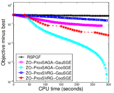
(a) 20news

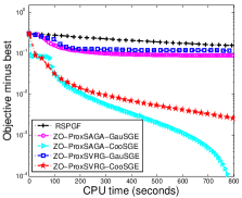
(b) a9a

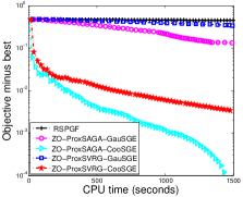
(c) w8a

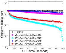
(d) covtype.binary

Figure 1: Objective value versus CPU time on black-box binary classification.

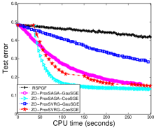
(a) 20news

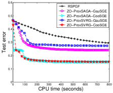
(b) a9a

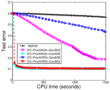
(c) w8a

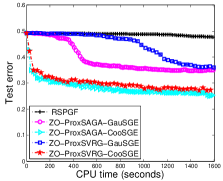
(d) covtype.binary

Figure 2: Test loss versus CPU time on black-box binary classification.

Experimental Results

Figures 1 and 2 show that both objective values and test losses of the proposed methods faster decrease than the RSPGF method, as the time increases. In particular, both the ZO-ProxSVRG and ZO-ProxSAGA using the CooSGE show the better performances than the counterparts using the GauSGE. From these results, we find that the CooSGE shows the better performances than the CauSGE in estimating gradients. Moreover, these results also demonstrate that both the ZO-ProxSVRG and ZO-ProxSAGA using the CooSGE have a relatively faster convergence rate than the counterparts using the GauSGE. Since the ZO-ProxSAGA has less function query complexity than the ZO-ProxSVRG, it shows the better performances than the ZO-ProxSVRG. For example, the ZO-ProxSVRG-CooSGE needs $O(ndS+bdT)$ function queries, while ZO-SAGA-CooSGE needs $O(bdT)$ function queries.

Adversarial Attacks on Black-Box DNNs

In this experiment, we apply our methods to generate adversarial examples to attack a pre-trained neural network model. Following (Chen et al., 2017; Liu et al., 2018c), the parameters of given model are hidden from us and only its outputs are accessible. In this case, we can not compute the gradients by using back-propagation algorithm. Thus, we use the zeroth-order algorithms to find an universal adversarial perturbation $x\in\mathbb{R}^{d}$ that could fool the samples $\{a_{i}\in\mathbb{R}^{d},\ l_{i}\in\mathbb{N}\}_{i=1}^{n}$, which can be specified as the following elastic-net attacks to black-box DNNs problem:

$$\min_{x\in\mathbb{R}^{d}} \frac{1}{n}\sum\limits_{i=1}^{n}\max\big{\{}F_{l_{i}}(a_{i}+x)-\max\limits_{j\neq l_{i}}F_{j}(a_{i}+x),0\big{\}}$$

$$+\lambda_{1}\left\|x\right\|_{1}+\lambda_{2}\left\|x\right\|_{2}^{2},$$ (31)

where $\lambda_{1}$ and $\lambda_{2}$ are nonnegative parameters to balance attack success rate, distortion and sparsity. Here $F(a)=[F_{1}(a),\cdots,F_{K}(a)]\in[0,1]^{K}$ represents the final layer output of neural network, which is the probabilities of $K$ classes.

Following (Liu et al., 2018c), we use a pre-trained DNN on the MNIST dataset as the target black-box model, which achieves 99.4$\%$ test accuracy. In the experiment, we select $n=10$ examples from the same class, and set the batch size $b=5$ and a constant step size $\eta=1/d$ for the zeroth-order algorithms, where $d=28\times 28$. In addition, we set $\lambda_{1}=10^{-3}$ and $\lambda_{2}=1$ in the experiment.

Figure 3 shows that both objective values and black-box attack losses (i.e. the first part of the problem (Adversarial Attacks on Black-Box DNNs)) of the proposed algorithms faster decrease than the RSPGF method, as the number of iteration increases. Here, we add the ZO-ProxSGD-CooSGE method for comparison, which is obtained by combining the ZO-ProxSGD method with the CooSGE. Interestingly, the ZO-ProxSGD-CooSGE shows better performance than both the ZO-ProxSVRG-GauSGE and ZO-ProxSAGA-GauSGE, which further demonstrates that the CooSGE can have better performance than the CauSGE in estimating gradient. Although having a relatively good performance in generating the adversarial samples, the ZO-ProxSGD still shows worse performance than both the ZO-ProxSVRG-CooSGE and ZO-ProxSAGA-CooSGE, due to not using the VR technique.

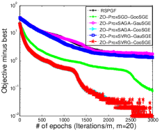
(a) Objective function value

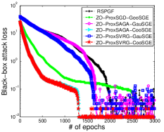
(b) Black-box attack loss

Figure 3: Objective value and attack loss on generating adversarial samples from black-box DNNs.

Conclusions

In this paper, we proposed a class of faster gradient-free proximal stochastic methods based on the zeroth-order gradient estimators, i.e., the GauSGE and the CooSGE, which only use the objective function values in the optimization. Moreover, we provided the theoretical analysis on the convergence properties of the proposed algorithms (ZO-ProxSVRG and ZO-ProxSAGA) based on the CooSGE and the GauSGE, respectively. In particular, both the ZO-ProxSVRG and ZO-ProxSAGA using the CooSGE have relatively faster convergence rates than the counterparts using the GauSGE, since the CooSGE has better performance than the CauSGE in estimating gradients.

Appendix A Supplementary Materials for “Faster Gradient-Free Proximal Stochastic Methods for Nonconvex Nonsmooth Optimization”

In this section, we provide the detailed proofs of the above lemmas and theorems. First, we give some useful properties of the CooSGE and the GauSGE, respectively.

Lemma 5.

(Liu et al., 2018c) Assume that the function $f(x)$ is $L$-smooth. Let $\hat{\nabla}f(x)$ denote the estimated gradient defined by the CooSGE. Define $f_{\mu_{j}}=\mathbb{E}_{u\sim U[-\mu_{j},\mu_{j}]}f(x+ue_{j})$, where $U[-\mu_{j},\mu_{j}]$ denotes the uniform distribution at the interval $[-\mu_{j},\mu_{j}]$. Then we have

• $f_{\mu_{j}}$ is $L$-smooth, and

  $$\hat{\nabla}f(x)=\sum_{j=1}^{d}\frac{\partial f_{\mu_{j}}(x)}{\partial x_{j}}e_{j},$$ (32)

  where $\partial f/\partial x_{j}$ denotes the partial derivative with respect to the $j$th coordinate.

• For $j\in[d]$,

  $$|f_{\mu_{j}}(x)-f(x)|\leq\frac{L\mu_{j}^{2}}{2},$$ (33)

  $$|\frac{\partial f_{\mu_{j}}(x)}{\partial x_{j}}|\leq\frac{L\mu_{j}^{2}}{2}.$$ (34)

• If $\mu=\mu_{j}$ for $j\in[d]$, then

  $$\|\hat{\nabla}f(x)-\nabla f(x)\|^{2}_{2}\leq\frac{L^{2}d^{2}\mu^{2}}{4}.$$ (35)

Lemma 6.

Assume that the function $f(x)$ is $L$-smooth. Let $\hat{\nabla}f(x)$ denote the estimated gradient defined by the GauSGE. Define $f_{\mu}(x)=\mathbb{E}_{u\sim\mathcal{N}(0,I)}[f(x+\mu u)]$. Then we have

• For any $x\in\mathbb{R}^{d}$, $\nabla f_{\mu}(x)=\mathbb{E}_{u}[\hat{\nabla}f(x)]$.

• For any $x\in\mathbb{R}^{d}$,

  $$|f_{\mu}(x)-f(x)|\leq\frac{Ld\mu^{2}}{2},$$

  $$|\nabla f_{\mu}(x)-\nabla f(x)|\leq\frac{L\mu(d+3)^{\frac{3}{2}}}{2},$$

  $$\mathbb{E}_{u}\|\hat{\nabla}f(x)\|^{2}\leq 2(d+4)\|\nabla f(x)\|^{2}+\frac{\mu^{2}L^{2}(d+6)^{3}}{2}.$$ (36)

• For any $x\in\mathbb{R}^{d}$,

  $$\mathbb{E}_{u}\|\hat{\nabla}f(x)-\nabla f(x)\|^{2}\leq 2(2d+9)\|\nabla f(x)\|^{2}+\mu^{2}L^{2}(d+6)^{3}.$$ (37)

Proof.

The first and second parts of the above results can be obtain from Lemma 5 in (Ghadimi, Lan, and Zhang, 2016). Using the inequality (36), we have

$$\|\hat{\nabla}f(x)-\nabla f(x)\|^{2} \leq 2\|\hat{\nabla}f(x)\|^{2}+2\|\nabla f(x)\|^{2}$$

$$\leq 2(2d+9)\|\nabla f(x)\|^{2}+\mu^{2}L^{2}(d+6)^{3},$$

where the first inequality holds by the Cauchy-Schwarz and Young’s inequality. ∎

Notations: To make the paper easier to follow, we give the following notations:

• $\|\cdot\|$ denotes the vector $\ell_{2}$ norm and the matrix spectral norm, respectively.

• $\mu$ denotes the smooth parameter of the gradient estimators (i.e., the CooSGE and GauSGE ).

• $\eta$ denotes the step size of updating variable $x$.

• $L$ denotes the Lipschitz constant of $\nabla f(x)$.

• $b$ denotes the mini-batch size of stochastic gradient.

• $T$, $m$ and $S$ are the total number of iterations, the number of iterations in the inner loop, and the number of iterations in the outer loop, respectively.

• For notational simplicity, $\mathbb{E}$ denotes $\mathbb{E}_{\mathcal{I}_{t},u}$.

Convergence Analysis of ZO-ProxSVRG-CooSGE

In this section, we give the convergence analysis of the ZO-ProxSVRG-CooSGE. First, we give an useful lemma about the upper bound of the variance of estimated gradient.

Lemma 7.

In Algorithm 1 using the CooSGE, given the estimated gradient $\hat{v}^{s}_{t}=\hat{\nabla}f_{\mathcal{I}_{t}}(x_{t}^{s})-\hat{\nabla}f_{\mathcal{I}_{t}}(\tilde{x}^{s})+\hat{\nabla}f(\tilde{x}^{s})$, then the following inequality holds

$$\mathbb{E}\|\hat{v}^{s}_{t}-\nabla f(x^{s}_{t})\|^{2}\leq\frac{2\delta_{n}L^{2}d}{b}\mathbb{E}\|x^{s}_{t}-\tilde{x}^{s}\|^{2}_{2}+\frac{L^{2}d^{2}\mu^{2}}{2}.$$ (38)

Proof.

Since

$$\mathbb{E}_{\mathcal{I}_{t}}[\hat{\nabla}f_{\mathcal{I}_{t}}(x_{t}^{s})-\hat{\nabla}f_{\mathcal{I}_{t}}(\tilde{x}^{s})]=\hat{\nabla}f(x_{t}^{s})-\hat{\nabla}f(\tilde{x}^{s}),$$ (39)

we have

$$\mathbb{E}\|\hat{v}^{s}_{t}-\nabla f(x^{s}_{t})\|^{2} =\mathbb{E}\|\hat{\nabla}f_{\mathcal{I}_{t}}(x_{t}^{s})-\hat{\nabla}f_{\mathcal{I}_{t}}(\tilde{x}^{s})+\hat{\nabla}f(\tilde{x}^{s})-\nabla f(x^{s}_{t})\|^{2}$$

$$=\mathbb{E}\|\hat{\nabla}f_{\mathcal{I}_{t}}(x_{t}^{s})-\hat{\nabla}f_{\mathcal{I}_{t}}(\tilde{x}^{s})+\hat{\nabla}f(\tilde{x}^{s})-\hat{\nabla}f(x_{t}^{s})+\hat{\nabla}f(x_{t}^{s})-\nabla f(x^{s}_{t})\|^{2}$$

$$=\mathbb{E}\|\hat{\nabla}f_{\mathcal{I}_{t}}(x_{t}^{s})-\hat{\nabla}f_{\mathcal{I}_{t}}(\tilde{x}^{s})-\mathbb{E}_{\mathcal{I}_{t}}(\hat{\nabla}f_{\mathcal{I}_{t}}(x_{t}^{s})-\hat{\nabla}f_{\mathcal{I}_{t}}(\tilde{x}^{s}))+\hat{\nabla}f(x_{t}^{s})-\nabla f(x^{s}_{t})\|^{2}$$

$$\leq 2\mathbb{E}\|\hat{\nabla}f_{\mathcal{I}_{t}}(x_{t}^{s})-\hat{\nabla}f_{\mathcal{I}_{t}}(\tilde{x}^{s})-\mathbb{E}_{\mathcal{I}_{t}}(\hat{\nabla}f_{\mathcal{I}_{t}}(x_{t}^{s})-\hat{\nabla}f_{\mathcal{I}_{t}}(\tilde{x}^{s}))\|^{2}+2\mathbb{E}\|\hat{\nabla}f(x_{t}^{s})-\nabla f(x^{s}_{t})\|^{2}$$

$$\leq 2\mathbb{E}\|\hat{\nabla}f_{\mathcal{I}_{t}}(x_{t}^{s})-\hat{\nabla}f_{\mathcal{I}_{t}}(\tilde{x}^{s})-\mathbb{E}_{\mathcal{I}_{t}}(\hat{\nabla}f_{\mathcal{I}_{t}}(x_{t}^{s})-\hat{\nabla}f_{\mathcal{I}_{t}}(\tilde{x}^{s}))\|^{2}+\frac{L^{2}d^{2}\mu^{2}}{2},$$ (40)

where the second inequality holds by Lemma 5. By the equality (39), we have

$$\sum_{i=1}^{n}\big{(}\hat{\nabla}f_{i}(x_{t}^{s})-\hat{\nabla}f_{i}(\tilde{x}^{s})-\mathbb{E}_{\mathcal{I}_{t}}(\hat{\nabla}f_{\mathcal{I}_{t}}(x_{t}^{s})-\hat{\nabla}f_{\mathcal{I}_{t}}(\tilde{x}^{s}))\big{)} =n\big{(}\hat{\nabla}f(x_{t}^{s})-\hat{\nabla}f(\tilde{x}^{s})\big{)}-n\big{(}\hat{\nabla}f(x_{t}^{s})-\hat{\nabla}f(\tilde{x}^{s})\big{)}$$

$$=0.$$ (41)

Based on (A), we have

$$\mathbb{E}\|\hat{\nabla}f_{\mathcal{I}_{t}}(x_{t}^{s})-\hat{\nabla}f_{\mathcal{I}_{t}}(\tilde{x}^{s})-\mathbb{E}_{\mathcal{I}_{t}}(\hat{\nabla}f_{\mathcal{I}_{t}}(x_{t}^{s})-\hat{\nabla}f_{\mathcal{I}_{t}}(\tilde{x}^{s}))\|^{2}$$

$$\leq\frac{\delta_{n}}{bn}\sum_{i=1}^{n}\mathbb{E}\|\hat{\nabla}f_{i}(x^{s}_{t})-\hat{\nabla}f_{i}(\tilde{x}^{s})-(\hat{\nabla}f(x^{s}_{t})-\hat{\nabla}f(\tilde{x}^{s}))\|^{2}$$

$$=\frac{\delta_{n}}{bn}\sum_{i=1}^{n}\mathbb{E}\|\hat{\nabla}f_{i}(x^{s}_{t})-\hat{\nabla}f_{i}(\tilde{x}^{s})\|^{2}\ -\|\hat{\nabla}f(x^{s}_{t})-\hat{\nabla}f(\tilde{x}^{s})\|^{2}$$

$$\leq\frac{\delta_{n}}{bn}\sum_{i=1}^{n}\mathbb{E}\|\hat{\nabla}f_{i}(x^{s}_{t})-\hat{\nabla}f_{i}(\tilde{x}^{s})\|^{2},$$ (42)

where the first inequality holds by Lemmas 4 and 5 in (Liu et al., 2018c), and

$$\delta_{n}=\left\{\begin{aligned} &1,\quad\mbox{if $\mathcal{I}_{t}$ contains i.i.d. samples with replacement}\\ &I(b<n),\mbox{if $\mathcal{I}_{t}$ contains i.i.d. samples without replacement},\end{aligned}\right.$$

$I(b<n)=1$ if $b<n$ and $0$ otherwise. Using (32), we have

$$\mathbb{E}\|\hat{\nabla}f_{i}(x^{s}_{t})-\hat{\nabla}f_{i}(\tilde{x}^{s})\|^{2} =\mathbb{E}\|\sum_{j=1}^{d}\frac{\partial f_{i,\mu_{j}}}{\partial x^{s}_{t,j}}e_{j}-\frac{\partial f_{i,\mu_{j}}}{\partial\tilde{x}^{s}_{j}}e_{j}\|^{2}$$

$$\leq d\sum_{j=1}^{d}\mathbb{E}\|\frac{\partial f_{i,\mu_{j}}}{\partial x^{s}_{t,j}}-\frac{\partial f_{i,\mu_{j}}}{\partial\tilde{x}^{s}_{j}}\|^{2}$$

$$\leq L^{2}d\sum_{j=1}^{d}\mathbb{E}\|x^{s}_{t,j}-\tilde{x}^{s}_{j}\|^{2}=L^{2}d\|x^{s}_{t}-\tilde{x}^{s}\|^{2},$$ (43)

where the first inequality holds by the Jensen’s inequality yielding $\|\frac{1}{n}\sum_{i=1}^{n}z_{i}\|^{2}\leq\frac{1}{n}\sum_{i=1}^{n}\|z_{i}\|^{2}$, and the second inequality holds due to that the function $f_{\mu_{j}}$ is $L$-smooth. Finally, combining the inequalities (A), (A) and (A), we have the above result.

∎

Next, based on the above lemma, we study the convergence property of the ZO-ProxSVRG-CooSGE.

Theorem 5.

Assume the sequence $\{(x^{s}_{t})_{t=1}^{m}\}_{s=1}^{S}$ generated from Algorithm 1 using the CooSGE, and given a sequence $\{c_{t}\}_{t=1}^{m}$ as follows: for $s=1,2,\cdots,S$

$$c_{t}=\left\{\begin{aligned} &\frac{\delta_{n}L^{2}d\eta}{b}+c_{t+1}(1+\beta),\ 0\leq t\leq m-1;\\ &0,\ t=m\end{aligned}\right.$$ (44)

where $\beta>0$. Let $T=mS$, $\eta=\frac{\rho}{dL}\ (0<\rho<\frac{1}{2})$ and $b$ satisfies the following inequality:

$$\frac{8\rho^{2}m^{2}}{b}+\rho\leq 1,$$ (45)

then we have

$$\mathbb{E}\|g_{\eta}(x^{s}_{t})\|^{2}\leq\frac{\mathbb{E}[F(x^{1}_{0})-F(x_{*})]}{T\gamma}+\frac{L^{2}d^{2}\mu^{2}\eta}{4\gamma},$$ (46)

where $\gamma=\frac{\eta}{2}-L\eta^{2}$ and $x^{*}$ is an optimal solution of the problem (2). Further let $b=[n^{\frac{2}{3}}]$, $m=[n^{\frac{1}{4}}]$, $\rho=\frac{1}{4}$ and $\mu=O(\frac{1}{\sqrt{dT}})$, we have

$$\mathbb{E}\|g_{\eta}(x^{s}_{t})\|^{2}\leq\frac{16dL\mathbb{E}[F(x^{1}_{0})-F(x_{*})]}{T}+O(\frac{d}{T}).$$ (47)

Proof.

We begin with defining an iteration by using the full true gradient:

$$\bar{x}^{s}_{t+1}=\mbox{Prox}_{\eta\psi}\big{(}x^{s}_{t}-\eta\nabla f(x^{s}_{t})\big{)}.$$ (48)

Then applying Lemma 2 of Reddi et al. (2016), we have

$$F(\bar{x}^{s}_{t+1})\leq F(z)+(\frac{L}{2}-\frac{1}{2\eta})\|\bar{x}^{s}_{t+1}-x^{s}_{t}\|^{2}+(\frac{L}{2}+\frac{1}{2\eta})\|z-x^{s}_{t}\|^{2}-\frac{1}{2\eta}\|\bar{x}^{s}_{t+1}-z\|^{2},\quad\forall z\in\mathbb{R}^{d}.$$ (49)

Since $x^{s}_{t+1}=\mbox{Prox}_{\eta\psi}\big{(}x^{s}_{t}-\eta\hat{v}^{s}_{t}\big{)}$, we have

$$F(x^{s}_{t+1})\leq F(z)+\langle x^{s}_{t+1}-z,\nabla f(x^{s}_{t})-\hat{v}^{s}_{t}\rangle+(\frac{L}{2}-\frac{1}{2\eta})\|x^{s}_{t+1}-x^{s}_{t}\|^{2}+(\frac{L}{2}+\frac{1}{2\eta})\|z-x^{s}_{t}\|^{2}-\frac{1}{2\eta}\|x^{s}_{t+1}-z\|^{2}.$$ (50)

Setting $z=x^{s}_{t}$ in (49) and $z=\bar{x}^{s}_{t+1}$ in (50), then summing them together and taking the expectations, we have

$$\mathbb{E}[F(x^{s}_{t+1})]\leq \mathbb{E}\big{[}F(x^{s}_{t})+\underbrace{\langle x^{s}_{t+1}-\bar{x}^{s}_{t+1},\nabla f(x^{s}_{t})-\hat{v}^{s}_{t}\rangle}_{T_{1}}+(\frac{L}{2}-\frac{1}{2\eta})\|x^{s}_{t+1}-x^{s}_{t}\|^{2}$$

$$+(L-\frac{1}{2\eta})\|\bar{x}^{s}_{t+1}-x^{s}_{t}\|^{2}-\frac{1}{2\eta}\|x^{s}_{t+1}-\bar{x}^{s}_{t+1}\|^{2}\big{]}.$$ (51)

Next, we give an upper bound of the term $T_{1}$ as follows:

$$T_{1} =\mathbb{E}\langle x^{s}_{t+1}-\bar{x}^{s}_{t+1},\nabla f(x^{s}_{t})-\hat{v}^{s}_{t}\rangle$$

$$\leq\frac{1}{2\eta}\mathbb{E}\|x^{s}_{t+1}-\bar{x}^{s}_{t+1}\|^{2}+\frac{\eta}{2}\mathbb{E}\|\nabla f(x^{s}_{t})-\hat{v}^{s}_{t}\|^{2}$$

$$\leq\frac{1}{2\eta}\mathbb{E}\|x^{s}_{t+1}-\bar{x}^{s}_{t+1}\|^{2}+\frac{\delta_{n}L^{2}d\eta}{b}\mathbb{E}\|x^{s}_{t}-\tilde{x}^{s}\|^{2}_{2}+\frac{L^{2}d^{2}\mu^{2}\eta}{4},$$ (52)

where the first inequality holds by Cauchy-Schwarz and Young’s inequality and the second inequality holds by Lemma 7. Combining (A) with (A), we have

$$\mathbb{E}[F(x^{s}_{t+1})]\leq \mathbb{E}\big{[}F(x^{s}_{t})+\frac{\delta_{n}L^{2}d\eta}{b}\mathbb{E}\|x^{s}_{t}-\tilde{x}^{s}\|^{2}_{2}+\frac{L^{2}d^{2}\mu^{2}\eta}{4}+(\frac{L}{2}-\frac{1}{2\eta})\|x^{s}_{t+1}-x^{s}_{t}\|^{2}$$

$$+(L-\frac{1}{2\eta})\|\bar{x}^{s}_{t+1}-x^{s}_{t}\|^{2}\big{]}.$$ (53)

Next, we define an useful Lyapunov function as follows:

$$R^{s}_{t}=\mathbb{E}\big{[}F(x^{s}_{t})+c_{t}\|x^{s}_{t}-\tilde{x}^{s}\|^{2}\big{]},$$ (54)

where $\{c_{t}\}$ is a nonnegative sequence. Considering the upper bound of $\|x^{s}_{t+1}-\tilde{x}^{s}\|^{2}$, we have

$$\|x^{s}_{t+1}-\tilde{x}^{s}\|^{2} =\|x^{s}_{t+1}-x^{s}_{t}+x^{s}_{t}-\tilde{x}^{s}\|^{2}$$

$$=\|x^{s}_{t+1}-x^{s}_{t}\|^{2}+2(x^{s}_{t+1}-x^{s}_{t})^{T}(x^{s}_{t}-\tilde{x}^{s})+\|x^{s}_{t}-\tilde{x}^{s}\|^{2}$$

$$\leq\|x^{s}_{t+1}-x^{s}_{t}\|^{2}+2\big{(}\frac{1}{2\beta}\|x^{s}_{t+1}-x^{s}_{t})\|^{2}+\frac{\beta}{2}\|x^{s}_{t}-\tilde{x}^{s}\|^{2}\big{)}+\|x^{s}_{t}-\tilde{x}^{s}\|^{2}$$

$$=(1+\frac{1}{\beta})\|x^{s}_{t+1}-x^{s}_{t}\|^{2}+(1+\beta)\|x^{s}_{t}-\tilde{x}^{s}\|^{2},$$ (55)

where $\beta>0$. Then we have

$$R^{s}_{t+1} =\mathbb{E}\big{[}F(x^{s}_{t+1})+c_{t+1}\|x^{s}_{t+1}-\tilde{x}^{s}\|^{2}\big{]}$$

$$\leq\mathbb{E}\big{[}F(x^{s}_{t+1})+c_{t+1}(1+\frac{1}{\beta})\|x^{s}_{t+1}-x^{s}_{t}\|^{2}+c_{t+1}(1+\beta)\|x^{s}_{t+1}-\tilde{x}^{s}\|^{2}\big{]}$$

$$\leq\mathbb{E}\big{[}F(x^{s}_{t})+\big{(}\frac{\delta_{n}L^{2}d\eta}{b}+c_{t+1}(1+\beta)\big{)}\|x^{s}_{t}-\tilde{x}^{s}\|^{2}+(L-\frac{1}{2\eta})\|\bar{x}^{s}_{t+1}-x^{s}_{t}\|^{2}$$

$$\quad+\big{(}\frac{L}{2}-\frac{1}{2\eta}+c_{t+1}(1+\frac{1}{\beta})\big{)}\|x^{s}_{t+1}-x^{s}_{t}\|^{2}+\frac{L^{2}d^{2}\mu^{2}\eta}{4}\big{]}$$

$$=R^{s}_{t}+(L-\frac{1}{2\eta})\|\bar{x}^{s}_{t+1}-x^{s}_{t}\|^{2}+\big{(}\frac{L}{2}-\frac{1}{2\eta}+c_{t+1}(1+\frac{1}{\beta})\big{)}\|x^{s}_{t+1}-x^{s}_{t}\|^{2}+\frac{L^{2}d^{2}\mu^{2}\eta}{4},$$ (56)

where $c_{t}=\frac{\delta_{n}L^{2}d\eta}{b}+c_{t+1}(1+\beta)$. Let $c_{m}=0$, $\beta=\frac{1}{m}$ and $\eta=\frac{\rho}{dL}(0<\rho<\frac{1}{2})$ , recursing on $t$, we have

$$c_{t}=\frac{\delta_{n}L^{2}d\eta}{b}\frac{(1+\beta)^{m-t}-1}{\beta} =\frac{\delta_{n}L\rho m}{b}\big{(}(1+\frac{1}{m})^{m-t}-1\big{)}$$

$$\leq\frac{\delta_{n}L\rho m}{b}(e-1)\leq\frac{2L\rho m}{b},$$ (57)

where the first inequality holds by $(1+\frac{1}{m})^{m}$ is an increasing function and $\lim_{m\rightarrow\infty}(1+\frac{1}{m})^{m}=e$; The second inequality holds by $0\leq\delta_{n}\leq 1$ and $e-1\leq 2$. It follows that

$$\frac{L}{2}+c_{t+1}(1+\frac{1}{\beta}) \leq\frac{L}{2}+\frac{2L\rho m}{b}(1+m)$$

$$\leq\frac{L}{2}+\frac{4L\rho m^{2}}{b}=(\rho+\frac{8\rho^{2}m^{2}}{b})\frac{L}{2\rho}\leq\frac{L}{2\rho}\leq\frac{1}{2\eta},$$ (58)

where the last inequality holds by $\rho+\frac{8\rho^{2}m^{2}}{b}\leq 1$. Thus, we have $\frac{L}{2}-\frac{1}{2\eta}+c_{t+1}(1+\frac{1}{\beta})\geq 0$. Then, we obtain

$$R^{s}_{t+1}\leq R^{s}_{t}+(L-\frac{1}{2\eta})\|\bar{x}^{s}_{t+1}-x^{s}_{t}\|^{2}+\frac{L^{2}d^{2}\mu^{2}\eta}{4}.$$ (59)

Telescoping inequality (59) over $t$ from $0$ to $m-1$, since $x^{s}_{0}=x^{s-1}_{m}=\tilde{x}^{s-1}$ and $x^{s}_{m}=\tilde{x}^{s}$, we have

$$\frac{1}{m}\sum_{t=1}^{m}\mathbb{E}\|g_{\eta}(x^{s}_{t})\|^{2}\leq\frac{\mathbb{E}[F(\tilde{x}^{s-1})-F(\tilde{x}^{s})]}{m\gamma}+\frac{L^{2}d^{2}\mu^{2}\eta}{4\gamma},$$ (60)

where $\gamma=\frac{\eta}{2}-\eta^{2}L$, and

$$g_{\eta}(x^{s}_{t})=\frac{1}{\eta}\big{[}x^{s}_{t}-\mbox{Prox}_{\eta\psi}(x^{s}_{t}-\eta\nabla f(x^{s}_{t}))\big{]}=\frac{1}{\eta}(x^{s}_{t}-\bar{x}^{s}_{t+1}).$$ (61)

Summing the inequality (60) over $s$ from $1$ to $S$, we have

$$\min_{t,s}\mathbb{E}\|g_{\eta}(x^{s}_{t})\|^{2}\leq\frac{1}{T}\sum_{s=1}^{S}\sum_{t=1}^{m}\mathbb{E}\|g_{\eta}(x^{s}_{t})\|^{2} \leq\frac{\mathbb{E}[F(\tilde{x}^{0})-F(\tilde{x}^{S})]}{T\gamma}+\frac{L^{2}d^{2}\mu^{2}\eta}{4\gamma}$$

$$\leq\frac{\mathbb{E}[F(\tilde{x}^{0})-F(x_{*})]}{T\gamma}+\frac{L^{2}d^{2}\mu^{2}\eta}{4\gamma},$$ (62)

where $x_{*}$ is an optimal solution of (2).

Given $m=[n^{\frac{1}{3}}]$, $b=[n^{\frac{2}{3}}]$ and $\rho=\frac{1}{4}$, it is easy verified that $\rho+\frac{8\rho^{2}m^{2}}{b}=\frac{3}{4}<1$. Using $d\geq 1$, we have $\gamma=\frac{\eta}{2}-L\eta^{2}=\frac{1}{8dL}-\frac{1}{16d^{2}L}\leq\frac{1}{8dL}-\frac{1}{16dL}=\frac{1}{16dL}$, we can obtain the above results.

∎

Convergence Analysis of ZO-ProxSVRG-GauSGE

In this section, we give the convergence analysis of the ZO-ProxSVRG-GauSGE. First, we give an useful lemma about the upper bound of the variance of estimated gradient.

Lemma 8.

In Algorithm 1 using GauSGE, given the estimated gradient $\hat{v}^{s}_{t}=\hat{\nabla}f_{\mathcal{I}_{t}}(x_{t}^{s})-\hat{\nabla}f_{\mathcal{I}_{t}}(\tilde{x}^{s})+\hat{\nabla}f(\tilde{x}^{s})$, then the following inequality holds

$$\mathbb{E}\|\hat{v}^{s}_{t}-\nabla f(x^{s}_{t})\|^{2}\leq \frac{6\delta_{n}L^{2}}{b}\mathbb{E}\|x^{s}_{t}-\tilde{x}^{s}\|^{2}+(2+\frac{12\delta_{n}}{b})L^{2}\mu^{2}(d+6)^{3}$$

$$+(4+\frac{24\delta_{n}}{b})(2d+9)\sigma^{2}.$$ (63)

Proof.

Since

$$\mathbb{E}_{\mathcal{I}_{t}}[\hat{\nabla}f_{\mathcal{I}_{t}}(x_{t}^{s})-\hat{\nabla}f_{\mathcal{I}_{t}}(\tilde{x}^{s})]=\hat{\nabla}f(x_{t}^{s})-\hat{\nabla}f(\tilde{x}^{s}),$$ (64)

we have

$$\mathbb{E}\|\hat{v}^{s}_{t}-\nabla f(x^{s}_{t})\|^{2} =\|\hat{\nabla}f_{\mathcal{I}_{t}}(x_{t}^{s})-\hat{\nabla}f_{\mathcal{I}_{t}}(\tilde{x}^{s})+\hat{\nabla}f(\tilde{x}^{s})-\nabla f(x^{s}_{t})\|^{2}$$ (65)

$$=\mathbb{E}\|\hat{\nabla}f_{\mathcal{I}_{t}}(x_{t}^{s})-\hat{\nabla}f_{\mathcal{I}_{t}}(\tilde{x}^{s})+\hat{\nabla}f(\tilde{x}^{s})-\hat{\nabla}f(x_{t}^{s})+\hat{\nabla}f(x_{t}^{s})-\nabla f(x^{s}_{t})\|^{2}$$

$$=\mathbb{E}\|\hat{\nabla}f_{\mathcal{I}_{t}}(x_{t}^{s})-\hat{\nabla}f_{\mathcal{I}_{t}}(\tilde{x}^{s})-\mathbb{E}_{\mathcal{I}_{t}}(\hat{\nabla}f_{\mathcal{I}_{t}}(x_{t}^{s})-\hat{\nabla}f_{\mathcal{I}_{t}}(\tilde{x}^{s}))+\hat{\nabla}f(x_{t}^{s})-\nabla f(x^{s}_{t})\|^{2}$$

$$\leq 2\mathbb{E}\|\hat{\nabla}f_{\mathcal{I}_{t}}(x_{t}^{s})-\hat{\nabla}f_{\mathcal{I}_{t}}(\tilde{x}^{s})-\mathbb{E}_{\mathcal{I}_{t}}(\hat{\nabla}f_{\mathcal{I}_{t}}(x_{t}^{s})-\hat{\nabla}f_{\mathcal{I}_{t}}(\tilde{x}^{s}))\|^{2}+2\mathbb{E}\|\hat{\nabla}f(x_{t}^{s})-\nabla f(x^{s}_{t})\|^{2}$$

$$\leq 2\mathbb{E}\|\hat{\nabla}f_{\mathcal{I}_{t}}(x_{t}^{s})-\hat{\nabla}f_{\mathcal{I}_{t}}(\tilde{x}^{s})-\mathbb{E}_{\mathcal{I}_{t}}(\hat{\nabla}f_{\mathcal{I}_{t}}(x_{t}^{s})-\hat{\nabla}f_{\mathcal{I}_{t}}(\tilde{x}^{s}))\|^{2}+4(2d+9)\|\nabla f(x^{s}_{t})\|^{2}+2\mu^{2}L^{2}(d+6)^{3},$$

$$\leq 2\mathbb{E}\|\hat{\nabla}f_{\mathcal{I}_{t}}(x_{t}^{s})-\hat{\nabla}f_{\mathcal{I}_{t}}(\tilde{x}^{s})-\mathbb{E}_{\mathcal{I}_{t}}(\hat{\nabla}f_{\mathcal{I}_{t}}(x_{t}^{s})-\hat{\nabla}f_{\mathcal{I}_{t}}(\tilde{x}^{s}))\|^{2}+4(2d+9)\sigma^{2}+2\mu^{2}L^{2}(d+6)^{3},$$

where the second inequality holds by Lemma 6 and the third inequality follows Assumption 2. By the equality (64), we have

$$\sum_{i=1}^{n}\big{(}\hat{\nabla}f_{i}(x_{t}^{s})-\hat{\nabla}f_{i}(\tilde{x}^{s})-\mathbb{E}_{\mathcal{I}_{t}}(\hat{\nabla}f_{\mathcal{I}_{t}}(x_{t}^{s})-\hat{\nabla}f_{\mathcal{I}_{t}}(\tilde{x}^{s}))\big{)} =n\big{(}\hat{\nabla}f(x_{t}^{s})-\hat{\nabla}f(\tilde{x}^{s})\big{)}-n\big{(}\hat{\nabla}f(x_{t}^{s})-\hat{\nabla}f(\tilde{x}^{s})\big{)}$$

$$=0.$$ (66)

It follows that

$$\mathbb{E}\|\hat{\nabla}f_{\mathcal{I}_{t}}(x_{t}^{s})-\hat{\nabla}f_{\mathcal{I}_{t}}(\tilde{x}^{s})-\mathbb{E}_{\mathcal{I}_{t}}(\hat{\nabla}f_{\mathcal{I}_{t}}(x_{t}^{s})-\hat{\nabla}f_{\mathcal{I}_{t}}(\tilde{x}^{s}))\|^{2}$$

$$\leq\frac{\delta_{n}}{bn}\sum_{i=1}^{n}\mathbb{E}\|\hat{\nabla}f_{i}(x^{s}_{t})-\hat{\nabla}f_{i}(\tilde{x}^{s})-(\hat{\nabla}f(x^{s}_{t})-\hat{\nabla}f(\tilde{x}^{s}))\|^{2}$$

$$=\frac{\delta_{n}}{bn}\sum_{i=1}^{n}\mathbb{E}[\|\hat{\nabla}f_{i}(x^{s}_{t})-\hat{\nabla}f_{i}(\tilde{x}^{s})\|^{2}\ -\|(\hat{\nabla}f(x^{s}_{t})-\hat{\nabla}f(\tilde{x}^{s}))\|^{2}$$

$$\leq\frac{\delta_{n}}{bn}\sum_{i=1}^{n}\mathbb{E}\|\hat{\nabla}f_{i}(x^{s}_{t})-\hat{\nabla}f_{i}(\tilde{x}^{s})\|^{2},$$ (67)

where the first inequality holds by Lemmas 4 and 5 in (Liu et al., 2018c). By (64), we have

$$\mathbb{E}\|\hat{\nabla}f_{i}(x^{s}_{t})-\hat{\nabla}f_{i}(\tilde{x}^{s})\|^{2} =\mathbb{E}\|\hat{\nabla}f_{i}(x^{s}_{t})-\nabla f_{i}(x^{s}_{t})+\nabla f_{i}(x^{s}_{t})-\nabla f_{i}(\tilde{x}^{s})+\nabla f_{i}(\tilde{x}^{s})-\hat{\nabla}f_{i}(\tilde{x}^{s})\|^{2}$$

$$\leq 3\mathbb{E}\|\hat{\nabla}f_{i}(x^{s}_{t})-\nabla f_{i}(x^{s}_{t})\|^{2}+3\|\nabla f_{i}(x^{s}_{t})-\nabla f_{i}(\tilde{x}^{s})\|^{2}+3\mathbb{E}\|\nabla f_{i}(\tilde{x}^{s})-\hat{\nabla}f_{i}(\tilde{x}^{s})\|^{2}$$

$$\leq 6(2d+9)\big{(}\|\nabla f_{i}(x^{s}_{t})\|^{2}+\|\nabla f_{i}(\tilde{x}^{s})\|^{2}\big{)}+3L^{2}\|x^{s}_{t}-\tilde{x}^{s}\|^{2}+6L^{2}\mu^{2}(d+6)^{3}$$

$$\leq 12(2d+9)\sigma^{2}+3L^{2}\|x^{s}_{t}-\tilde{x}^{s}\|^{2}+6L^{2}\mu^{2}(d+6)^{3},$$ (68)

where the first inequality holds by the Jensen’s inequality, the second inequality holds by the Lemma 6 and the third inequality follows Assumption 2. Finally, combining the inequalities (65), (A) and (A), we obtain the above result.

∎

Next, based on the above lemma, we study the convergence property of the ZO-ProxSVRG-GauSGE.

Theorem 6.

Assume the sequence $\{(x^{s}_{t})_{t=1}^{m}\}_{s=1}^{S}$ generated from Algorithm 1 using the GauSGE, and given a sequence $\{c_{t}\}_{t=1}^{m}$ as follows: for $s=1,2,\cdots,S$

$$c_{t}=\left\{\begin{aligned} &\frac{3\delta_{n}L^{2}\eta}{b}+c_{t+1}(1+\beta),\ 0\leq t\leq m-1;\\ &0,\ t=m\end{aligned}\right.$$ (69)

where $\beta>0$. Let $\eta=\frac{\rho}{L}\ (0<\rho<\frac{1}{2})$ and $b$ satisfies the following inequality:

$$\frac{24\rho^{2}m^{2}}{b}+\rho\leq 1,$$ (70)

then we have

$$\mathbb{E}\|g_{\eta}(x^{s}_{t})\|^{2}\leq\frac{\mathbb{E}[F(x^{1}_{0})-F(x_{*})]}{T\gamma}+(1+\frac{6\delta_{n}}{b})(d+6)^{3}\frac{L^{2}\mu^{2}\eta}{\gamma}+(2+\frac{12\delta_{n}}{b})(2d+9)\frac{\sigma^{2}\eta}{\gamma},$$ (71)

where $\gamma=\frac{\eta}{2}-\eta^{2}L$ and $x^{*}$ is an optimal solution of the problem (2). Further let $b=[n^{\frac{2}{3}}]$, $m=[n^{\frac{1}{3}}]$, $\rho=\frac{1}{6}$ and $\mu=O(\frac{1}{d\sqrt{T}})$, we have

$$\mathbb{E}\|g_{\eta}(x^{s}_{t})\|^{2}\leq\frac{18L\mathbb{E}[F(x^{1}_{0})-F(x_{*})]}{T}+O(\frac{d}{T})+O(d\sigma^{2}).$$ (72)

Proof.

This proof is the similar to the proof of Theorem 1. We start by defining an iteration by using the full true gradient:

$$\bar{x}^{s}_{t+1}=\mbox{Prox}_{\eta\psi}\big{(}x^{s}_{t}-\eta\nabla f(x^{s}_{t})\big{)},$$ (73)

then applying Lemma 2 of Reddi et al. (2016), we have

$$F(\bar{x}^{s}_{t+1})\leq F(z)+(\frac{L}{2}-\frac{1}{2\eta})\|\bar{x}^{s}_{t+1}-x^{s}_{t}\|^{2}+(\frac{L}{2}+\frac{1}{2\eta})\|z-x^{s}_{t}\|^{2}-\frac{1}{2\eta}\|\bar{x}^{s}_{t+1}-z\|^{2},\quad\forall z\in\mathbb{R}^{d}.$$ (74)

Since $x^{s}_{t+1}=\mbox{Prox}_{\eta\psi}\big{(}x^{s}_{t}-\eta\hat{v}^{s}_{t}\big{)}$, we have

$$F(x^{s}_{t+1})\leq F(z)+\langle x^{s}_{t+1}-z,\nabla f(x^{s}_{t})-\hat{v}^{s}_{t}\rangle+(\frac{L}{2}-\frac{1}{2\eta})\|x^{s}_{t+1}-x^{s}_{t}\|^{2}+(\frac{L}{2}+\frac{1}{2\eta})\|z-x^{s}_{t}\|^{2}-\frac{1}{2\eta}\|x^{s}_{t+1}-z\|^{2}.$$ (75)

Setting $z=x^{s}_{t}$ in (74) and $z=\bar{x}^{s}_{t+1}$ in (75), then summing them together and taking the expectations, we obtain

$$\mathbb{E}[F(x^{s}_{t+1})]\leq \mathbb{E}\big{[}F(x^{s}_{t})+\underbrace{\langle x^{s}_{t+1}-\bar{x}^{s}_{t+1},\nabla f(x^{s}_{t})-\hat{v}^{s}_{t}\rangle}_{T_{2}}+(\frac{L}{2}-\frac{1}{2\eta})\|x^{s}_{t+1}-x^{s}_{t}\|^{2}$$

$$+(L-\frac{1}{2\eta})\|\bar{x}^{s}_{t+1}-x^{s}_{t}\|^{2}-\frac{1}{2\eta}\|x^{s}_{t+1}-\bar{x}^{s}_{t+1}\|^{2}\big{]}.$$ (76)

Next, we give an upper bound of the term $T_{2}$ as follows:

$$T_{2} =\mathbb{E}\langle x^{s}_{t+1}-\bar{x}^{s}_{t+1},\nabla f(x^{s}_{t})-\hat{v}^{s}_{t}\rangle$$

$$\leq\frac{1}{2\eta}\mathbb{E}\|x^{s}_{t+1}-\bar{x}^{s}_{t+1}\|^{2}+\frac{\eta}{2}\mathbb{E}\|\nabla f(x^{s}_{t})-\hat{v}^{s}_{t}\|^{2}$$

$$\leq\frac{1}{2\eta}\mathbb{E}\|x^{s}_{t+1}-\bar{x}^{s}_{t+1}\|^{2}+\frac{3\delta_{n}L^{2}\eta}{b}\mathbb{E}\|x^{s}_{t}-\tilde{x}^{s}\|^{2}+(1+\frac{6\delta_{n}}{b})L^{2}(d+6)^{3}\mu^{2}\eta+(2+\frac{12\delta_{n}}{b})(2d+9)\sigma^{2}\eta,$$ (77)

where the first inequality holds by Cauchy-Schwarz and Young’s inequality and the second inequality holds by Lemma 8. Combining (A) with (A), we have

$$\mathbb{E}[F(x^{s}_{t+1})]\leq \mathbb{E}\big{[}F(x^{s}_{t})+\frac{3\delta_{n}L^{2}\eta}{b}\mathbb{E}\|x^{s}_{t}-\tilde{x}^{s}\|^{2}+(1+\frac{6\delta_{n}}{b})L^{2}(d+6)^{3}\mu^{2}\eta+(2+\frac{12\delta_{n}}{b})(2d+9)\sigma^{2}\eta$$

$$+(\frac{L}{2}-\frac{1}{2\eta})\|x^{s}_{t+1}-x^{s}_{t}\|^{2}+(L-\frac{1}{2\eta})\|\bar{x}^{s}_{t+1}-x^{s}_{t}\|^{2}\big{]}.$$ (78)

Next, we define an useful Lyapunov function as follows:

$$\Psi^{s}_{t}=\mathbb{E}\big{[}F(x^{s}_{t})+c_{t}\|x^{s}_{t}-\tilde{x}^{s}\|^{2}\big{]},$$ (79)

where $\{c_{t}\}$ is a nonnegative sequence. Considering the upper bound of $\|x^{s}_{t+1}-\tilde{x}^{s}\|^{2}$, we have

$$\|x^{s}_{t+1}-\tilde{x}^{s}\|^{2} =\|x^{s}_{t+1}-x^{s}_{t}+x^{s}_{t}-\tilde{x}^{s}\|^{2}$$

$$=\|x^{s}_{t+1}-x^{s}_{t}\|^{2}+2(x^{s}_{t+1}-x^{s}_{t})^{T}(x^{s}_{t}-\tilde{x}^{s})+\|x^{s}_{t}-\tilde{x}^{s}\|^{2}$$

$$\leq\|x^{s}_{t+1}-x^{s}_{t}\|^{2}+2\big{(}\frac{1}{2\beta}\|x^{s}_{t+1}-x^{s}_{t})\|^{2}+\frac{\beta}{2}\|x^{s}_{t}-\tilde{x}^{s}\|^{2}\big{)}+\|x^{s}_{t}-\tilde{x}^{s}\|^{2}$$

$$=(1+\frac{1}{\beta})\|x^{s}_{t+1}-x^{s}_{t}\|^{2}+(1+\beta)\|x^{s}_{t}-\tilde{x}^{s}\|^{2},$$ (80)

where $\beta>0$. Then we have

$$\Psi^{s}_{t+1} =\mathbb{E}\big{[}F(x^{s}_{t+1})+c_{t+1}\|x^{s}_{t+1}-\tilde{x}^{s}\|^{2}\big{]}$$

$$\leq\mathbb{E}\big{[}F(x^{s}_{t+1})+c_{t+1}(1+\frac{1}{\beta})\|x^{s}_{t+1}-x^{s}_{t}\|^{2}+c_{t+1}(1+\beta)\|x^{s}_{t+1}-\tilde{x}^{s}\|^{2}\big{]}$$

$$\leq\mathbb{E}\big{[}F(x^{s}_{t})+\big{(}\frac{3\delta_{n}L^{2}\eta}{b}+c_{t+1}(1+\beta)\big{)}\|x^{s}_{t}-\tilde{x}^{s}\|^{2}+(L-\frac{1}{2\eta})\|\bar{x}^{s}_{t+1}-x^{s}_{t}\|^{2}+\big{(}\frac{L}{2}-\frac{1}{2\eta}+c_{t+1}(1+\frac{1}{\beta})\big{)}\|x^{s}_{t+1}-x^{s}_{t}\|^{2}$$

$$\quad+(1+\frac{6\delta_{n}}{b})(d+6)^{3}L^{2}\mu^{2}\eta+(2+\frac{12\delta_{n}}{b})(2d+9)\sigma^{2}\eta\big{]}$$

$$=\Psi^{s}_{t}+(L-\frac{1}{2\eta})\|\bar{x}^{s}_{t+1}-x^{s}_{t}\|^{2}+\big{(}\frac{L}{2}-\frac{1}{2\eta}+c_{t+1}(1+\frac{1}{\beta})\big{)}\|x^{s}_{t+1}-x^{s}_{t}\|^{2}$$

$$\quad+(1+\frac{6\delta_{n}}{b})(d+6)^{3}L^{2}\mu^{2}\eta+(2+\frac{12\delta_{n}}{b})(2d+9)\sigma^{2}\eta,$$ (81)

where $c_{t}=\frac{3\delta_{n}L^{2}\eta}{b}+c_{t+1}(1+\beta)$. Let $c_{m}=0$, $\beta=\frac{1}{m}$ and $\eta=\frac{\rho}{L}(0<\rho<\frac{1}{2})$ , recursing on $t$, we have

$$c_{t}=\frac{3\delta_{n}L^{2}\eta}{b}\frac{(1+\beta)^{m-t}-1}{\beta} =\frac{3\delta_{n}L\rho m}{b}\big{(}(1+\frac{1}{m})^{m-t}-1\big{)}$$

$$\leq\frac{3\delta_{n}L\rho m}{b}(e-1)\leq\frac{6L\rho m}{b},$$ (82)

where the first inequality holds by $(1+\frac{1}{m})^{m}$ is an increasing function and $\lim_{m\rightarrow\infty}(1+\frac{1}{m})^{m}=e$.

It follows that

$$\frac{L}{2}+c_{t+1}(1+\frac{1}{\beta}) \leq\frac{L}{2}+\frac{6L\rho m}{b}(1+m)$$

$$\leq\frac{L}{2}+\frac{12L\rho m^{2}}{b}=(\rho+\frac{24\rho^{2}m^{2}}{b})\frac{L}{2\rho}\leq\frac{L}{2\rho}=\frac{1}{2\eta},$$ (83)

where the last inequality holds by $\rho+\frac{24\rho^{2}m^{2}}{b}\leq 1$. Then we obtain

$$\Psi^{s}_{t+1}\leq\Psi^{s}_{t}+(L-\frac{1}{2\eta})\|\bar{x}^{s}_{t+1}-x^{s}_{t}\|^{2}+(1+\frac{6\delta_{n}}{b})(d+6)^{3}L^{2}\mu^{2}\eta+(2+\frac{12\delta_{n}}{b})(2d+9)\sigma^{2}\eta.$$ (84)

Telescoping inequality (84) over $t$ from $0$ to $m-1$, since $x^{s}_{0}=x^{s-1}_{m}=\tilde{x}^{s-1}$ and $x^{s}_{m}=\tilde{x}^{s}$, we have

$$\frac{1}{m}\sum_{t=1}^{m}\mathbb{E}\|g_{\eta}(x^{s}_{t})\|^{2}\leq\frac{\mathbb{E}[F(\tilde{x}^{s-1})-F(\tilde{x}^{s})]}{m\gamma}+(1+\frac{6\delta_{n}}{b})(d+6)^{3}\frac{L^{2}\mu^{2}\eta}{\gamma}+(2+\frac{12\delta_{n}}{b})(2d+9)\frac{\sigma^{2}\eta}{\gamma},$$ (85)

where $\gamma=\frac{\eta}{2}-\eta^{2}L$, and

$$g_{\eta}(x^{s}_{t})=\frac{1}{\eta}\big{[}x^{s}_{t}-\mbox{Prox}_{\eta\psi}(x^{s}_{t}-\eta\nabla f(x^{s}_{t}))\big{]}=\frac{1}{\eta}(x^{s}_{t}-\bar{x}^{s}_{t+1}).$$ (86)

Summing the inequality (85) over $s$ from $1$ to $S$, we have

$$\frac{1}{T}\sum_{s=1}^{S}\sum_{t=1}^{m}\mathbb{E}\|g_{\eta}(x^{s}_{t})\|^{2} \leq\frac{\mathbb{E}[F(\tilde{x}^{0})-F(\tilde{x}^{S})]}{T\gamma}+(1+\frac{6\delta_{n}}{b})(d+6)^{3}\frac{L^{2}\mu^{2}\eta}{\gamma}+(2+\frac{12\delta_{n}}{b})(2d+9)\frac{\sigma^{2}\eta}{\gamma}$$

$$\leq\frac{\mathbb{E}[F(\tilde{x}^{0})-F(x_{*})]}{T\gamma}+(1+\frac{6\delta_{n}}{b})(d+6)^{3}\frac{L^{2}\mu^{2}\eta}{\gamma}+(2+\frac{12\delta_{n}}{b})(2d+9)\frac{\sigma^{2}\eta}{\gamma},$$ (87)

where $x_{*}$ is an optimal solution of (2).

Let $m=[n^{\frac{1}{3}}]$, $b=[n^{\frac{2}{3}}]$ and $\rho=\frac{1}{6}$, it is easy verified that $\rho+\frac{24\rho^{2}m^{2}}{b}=\frac{5}{6}<1$ and $\gamma=\frac{\eta}{2}-\eta^{2}L=\frac{1}{18L}$. Finally, given $\mu=O(\frac{1}{d\sqrt{T}})$, we can obtain the above results.

∎

Convergence Analysis of ZO-ProxSAGA-CooSGE

In this section, we give the convergence analysis of the ZO-ProxSAGA-CooSGE. First, we give an useful lemma about the upper bound of the variance of estimated gradient.

Lemma 9.

In Algorithm 2 using the CooSGE, given the estimated gradient $\hat{v}_{t}=\frac{1}{b}\sum_{i_{t}\in\mathcal{I}_{t}}\big{(}\hat{\nabla}f_{i_{t}}(x_{t})-\hat{\nabla}f_{i_{t}}(z^{t}_{i_{t}})\big{)}+\hat{\phi}_{t}$ with $\hat{\phi}_{t}=\frac{1}{n}\sum_{i=1}^{n}\hat{\nabla}f_{i}(z^{t}_{i})$, then the following inequality holds

$$\mathbb{E}\|\hat{v}_{t}-\nabla f(x_{t})\|^{2}\leq\frac{2L^{2}d}{nb}\sum_{i=1}^{n}\mathbb{E}\|x_{t}-z^{t}_{i}\|^{2}_{2}+\frac{L^{2}d^{2}\mu^{2}}{2}.$$ (88)

Proof.

By the definition of the estimated gradient $\hat{v}_{t}$, we have

$$\mathbb{E}\|\hat{v}_{t}-\nabla f(x^{s}_{t})\|^{2} =\mathbb{E}\|\frac{1}{b}\sum_{i_{t}\in\mathcal{I}_{t}}\big{(}\hat{\nabla}f_{i_{t}}(x_{t})-\hat{\nabla}f_{i_{t}}(z^{t}_{i_{t}})\big{)}+\hat{\phi}_{t}-\nabla f(x_{t})\|^{2}$$

$$=\mathbb{E}\|\frac{1}{b}\sum_{i_{t}\in\mathcal{I}_{t}}\big{(}\hat{\nabla}f_{i_{t}}(x_{t})-\hat{\nabla}f_{i_{t}}(z^{t}_{i_{t}})\big{)}+\hat{\phi}_{t}-\hat{\nabla}f(x_{t})+\hat{\nabla}f(x_{t})-\nabla f(x_{t})\|^{2}$$

$$\leq 2\mathbb{E}\|\frac{1}{b}\sum_{i_{t}\in\mathcal{I}_{t}}\big{(}\hat{\nabla}f_{i_{t}}(x_{t})-\hat{\nabla}f_{i_{t}}(z^{t}_{i_{t}})\big{)}+\hat{\phi}_{t}-\hat{\nabla}f(x_{t})\|^{2}+2\mathbb{E}\|\hat{\nabla}f(x_{t})-\nabla f(x_{t})\|^{2}$$

$$\leq 2\mathbb{E}\|\frac{1}{b}\sum_{i_{t}\in\mathcal{I}_{t}}\big{(}\hat{\nabla}f_{i_{t}}(x_{t})-\hat{\nabla}f_{i_{t}}(z^{t}_{i_{t}})\big{)}-(\hat{\nabla}f(x_{t})-\hat{\phi}_{t})\|^{2}+\frac{L^{2}d^{2}\mu^{2}}{2},$$ (89)

where the second inequality holds by Lemma 5. Using

$$\mathbb{E}_{\mathcal{I}_{t}}\big{[}\frac{1}{b}\sum_{i_{t}\in\mathcal{I}_{t}}\hat{\nabla}f_{i_{t}}(x_{t})-\hat{\nabla}f_{i_{t}}(z^{t}_{i_{t}})\big{]}=\hat{\nabla}f(x_{t})-\frac{1}{n}\sum_{i=1}^{n}\hat{\nabla}f_{i}(z^{t}_{i})=\hat{\nabla}f(x_{t})-\hat{\phi}_{t},$$ (90)

we have

$$\sum_{i=1}^{n}\big{(}\hat{\nabla}f_{i}(x_{t})-\hat{\nabla}f_{i}(z^{t}_{i_{t}})-(\hat{\nabla}f(x_{t})-\hat{\phi}_{t})\big{)}=n\big{(}\hat{\nabla}f(x_{t})-\hat{\phi}_{t}\big{)}-n\big{(}\hat{\nabla}f(x_{t})-\hat{\phi}_{t}\big{)}=0.$$ (91)

It follows that

$$\mathbb{E}\|\frac{1}{b}\sum_{i_{t}\in\mathcal{I}_{t}}\big{(}\hat{\nabla}f_{i_{t}}(x_{t})-\hat{\nabla}f_{i_{t}}(z^{t}_{i_{t}})\big{)}-(\hat{\nabla}f(x_{t})-\hat{\phi}_{t})\|^{2}$$

$$\leq\frac{1}{bn}\sum_{i=1}^{n}\mathbb{E}\|\hat{\nabla}f_{i}(x_{t})-\hat{\nabla}f_{i}(z^{t}_{i})-(\hat{\nabla}f(x_{t})-\hat{\phi}_{t})\|^{2}$$

$$=\frac{1}{bn}\sum_{i=1}^{n}\mathbb{E}\|\hat{\nabla}f_{i}(x_{t})-\hat{\nabla}f_{i}(z^{t}_{i})\|^{2}\ -\|\hat{\nabla}f(x_{t})-\hat{\phi}_{t}\|^{2}$$

$$\leq\frac{1}{bn}\sum_{i=1}^{n}\mathbb{E}\|\hat{\nabla}f_{i}(x_{t})-\hat{\nabla}f_{i}(z^{t}_{i})\|^{2},$$ (92)

where the first inequality holds by Lemmas 4 and 5 in (Liu et al., 2018c). By (32), we have

$$\mathbb{E}\|\hat{\nabla}f_{i}(x_{t})-\hat{\nabla}f_{i}(z^{t}_{i})\|^{2} =\mathbb{E}\|\sum_{j=1}^{d}\frac{\partial f_{i,\mu_{j}}}{\partial x_{t,j}}e_{j}-\frac{\partial f_{i,\mu_{j}}}{\partial z^{t}_{i,j}}e_{j}\|^{2}$$

$$\leq d\sum_{j=1}^{d}\mathbb{E}\|\frac{\partial f_{i,\mu_{j}}}{\partial x_{t,j}}-\frac{\partial f_{i,\mu_{j}}}{\partial z^{t}_{i,j}}\|^{2}$$

$$\leq L^{2}d\sum_{j=1}^{d}\mathbb{E}\|x_{t,j}-z^{t}_{i,j}\|^{2}=L^{2}d\|x_{t}-z^{t}_{i}\|^{2},$$ (93)

where the first inequality follows the Jensen’s inequality, and the second inequality holds due to that the function $f_{\mu_{j}}$ is $L$-smooth.

Finally, combining the inequalities (A), (A) and (A), we have the above result.

∎

Next, based on the above lemma, we study the convergence property of the ZO-ProxSAGA-CooSGE.

Theorem 7.

Assume the sequence $\{x_{t}\}_{t=1}^{T}$ generated from Algorithm 2 using the CooSGE, and given a positive sequence $\{c_{t}\}_{t=1}^{T}$ as follows:

$$c_{t}=\frac{L^{2}d\eta}{b}+c_{t+1}(1-p)(1+\beta)$$ (94)

where $\beta>0$. Let $c_{T}=0$, $\eta=\frac{\rho}{Ld}\ (0<\rho<\frac{1}{2})$, and $b$ satisfies the following inequality:

$$\frac{32\rho^{2}n^{2}}{b^{3}}+\rho\leq 1,$$ (95)

then we have

$$\mathbb{E}\|g_{\eta}(x_{t})\|^{2}\leq\frac{\mathbb{E}[F(x_{0})-F(x_{*})]}{T\gamma}+\frac{L^{2}d^{2}\mu^{2}\eta}{4\gamma},$$ (96)

where $\gamma=\frac{\eta}{2}-L\eta^{2}$ and $x^{*}$ is an optimal solution of the problem (2). Further let $b=[n^{\frac{2}{3}}]$, $\rho=\frac{1}{8}$ and $\mu=O(\frac{1}{\sqrt{dT}})$, we obtain

$$\mathbb{E}\|g_{\eta}(x_{t})\|^{2}\leq\frac{64dL\mathbb{E}[F(x_{0})-F(x_{*})]}{3T}+O(\frac{d}{T}).$$ (97)

Proof.

First, we define an iteration by using the full true gradient:

$$\bar{x}_{t+1}=\mbox{Prox}_{\eta\psi}\big{(}x_{t}-\eta\nabla f(x_{t})\big{)},$$ (98)

then applying Lemma 2 of Reddi et al. (2016), we have

$$F(\bar{x}_{t+1})\leq F(z)+(\frac{L}{2}-\frac{1}{2\eta})\|\bar{x}_{t+1}-x_{t}\|^{2}+(\frac{L}{2}+\frac{1}{2\eta})\|z-x_{t}\|^{2}-\frac{1}{2\eta}\|\bar{x}_{t+1}-z\|^{2},\quad\forall z\in\mathbb{R}^{d}.$$ (99)

Since $x_{t+1}=\mbox{Prox}_{\eta\psi}\big{(}x_{t}-\eta\hat{v}_{t}\big{)}$, we have

$$F(x_{t+1})\leq F(z)+\langle x_{t+1}-z,\nabla f(x_{t})-\hat{v}_{t}\rangle+(\frac{L}{2}-\frac{1}{2\eta})\|x_{t+1}-x_{t}\|^{2}+(\frac{L}{2}+\frac{1}{2\eta})\|z-x_{t}\|^{2}-\frac{1}{2\eta}\|x_{t+1}-z\|^{2}.$$ (100)

Setting $z=x_{t}$ in (99) and $z=\bar{x}_{t+1}$ in (100), then summing them together and taking the expectations, we obtain

$$\mathbb{E}[F(x_{t+1})]\leq \mathbb{E}\big{[}F(x_{t})+\underbrace{\langle x_{t+1}-\bar{x}_{t+1},\nabla f(x_{t})-\hat{v}_{t}\rangle}_{T_{3}}+(\frac{L}{2}-\frac{1}{2\eta})\|x_{t+1}-x_{t}\|^{2}$$

$$+(L-\frac{1}{2\eta})\|\bar{x}_{t+1}-x_{t}\|^{2}-\frac{1}{2\eta}\|x_{t+1}-\bar{x}_{t+1}\|^{2}\big{]}.$$ (101)

Next, we give an upper bound of the term $T_{3}$ as follows:

$$T_{3} =\mathbb{E}\langle x_{t+1}-\bar{x}_{t+1},\nabla f(x_{t})-\hat{v}_{t}\rangle$$

$$\leq\frac{1}{2\eta}\mathbb{E}\|x_{t+1}-\bar{x}_{t+1}\|^{2}+\frac{\eta}{2}\mathbb{E}\|\nabla f(x_{t})-\hat{v}_{t}\|^{2}$$

$$\leq\frac{1}{2\eta}\mathbb{E}\|x_{t+1}-\bar{x}_{t+1}\|^{2}+\frac{L^{2}d\eta}{nb}\sum_{i=1}^{n}\mathbb{E}\|x_{t}-z^{t}_{i}\|^{2}_{2}+\frac{L^{2}d^{2}\mu^{2}\eta}{4},$$ (102)

where the first inequality holds by Cauchy-Schwarz and Young’s inequality and the second inequality holds by Lemma 9.

Combining (A) with (A), we have

$$\mathbb{E}[F(x_{t+1})]\leq \mathbb{E}\big{[}F(x_{t})+\frac{L^{2}d\eta}{nb}\sum_{i=1}^{n}\mathbb{E}\|x_{t}-z^{t}_{i}\|^{2}_{2}+\frac{L^{2}d^{2}\mu^{2}\eta}{4}+(\frac{L}{2}-\frac{1}{2\eta})\|x_{t+1}-x_{t}\|^{2}$$

$$+(L-\frac{1}{2\eta})\|\bar{x}_{t+1}-x_{t}\|^{2}\big{]}.$$ (103)

Next, we define an useful Lyapunov function as follows:

$$\Phi_{t}=\mathbb{E}\big{[}F(x_{t})+c_{t}\frac{1}{n}\sum_{i=1}^{n}\|x_{t}-z^{t}_{i}\|^{2}\big{]},$$ (104)

where $\{c_{t}\}$ is a nonnegative sequence. By the step 7 of Algorithm 2, we have

$$\frac{1}{n}\sum_{i=1}^{n}\|x_{t+1}-z^{t+1}_{i}\|^{2} =\frac{1}{n}\sum_{i=1}^{n}\big{(}p\|x_{t+1}-x_{t}\|^{2}+(1-p)\|x_{t+1}-z^{t}_{i}\|^{2}\big{)}$$

$$=\frac{p}{n}\sum_{i=1}^{n}\|x_{t+1}-x_{t}\|^{2}+\frac{1-p}{n}\sum_{i=1}^{n}\|x_{t+1}-z^{t}_{i}\|^{2}$$

$$=p\|x_{t+1}-x_{t}\|^{2}+\frac{1-p}{n}\sum_{i=1}^{n}\|x_{t+1}-z^{t}_{i}\|^{2},$$ (105)

where $p$ denotes probability of an index $i$ being in $\mathcal{I}_{t}$. Here we have

$$p=1-(1-\frac{1}{n})^{b}\geq 1-\frac{1}{1+b/n}=\frac{b/n}{1+b/n}\geq\frac{b}{2n},$$ (106)

where the first inequality follows from $(1-a)^{b}\leq\frac{1}{1+ab}$, and the second inequality holds by $b\leq n$. Considering the upper bound of $\|x_{t+1}-z^{t}_{i}\|^{2}$, we have

$$\|x_{t+1}-z^{t}_{i}\|^{2} =\|x_{t+1}-x_{t}+x_{t}-z^{t}_{i}\|^{2}$$

$$=\|x_{t+1}-x_{t}\|^{2}+2(x_{t+1}-x_{t})^{T}(x_{t}-z^{t}_{i})+\|x_{t}-z^{t}_{i}\|^{2}$$

$$\leq\|x_{t+1}-x_{t}\|^{2}+2\big{(}\frac{1}{2\beta}\|x_{t+1}-x_{t}\|^{2}+\frac{\beta}{2}\|x_{t}-z^{t}_{i}\|^{2}\big{)}+\|x_{t}-z^{t}_{i}\|^{2}$$

$$=(1+\frac{1}{\beta})\|x_{t+1}-x_{t}\|^{2}+(1+\beta)\|x_{t}-z^{t}_{i}\|^{2},$$ (107)

where $\beta>0$. Combining (A) with (A), we have

$$\frac{1}{n}\sum_{i=1}^{n}\|x_{t+1}-z^{t+1}_{i}\|^{2}\leq(1+\frac{1-p}{\beta})\|x_{t+1}-x_{t}\|^{2}+\frac{(1-p)(1+\beta)}{n}\sum_{i=1}^{n}\|x_{t}-z^{t}_{i}\|^{2}.$$ (108)

It follows that

$$\Phi_{t+1} =\mathbb{E}\big{[}F(x_{t+1})+c_{t+1}\frac{1}{n}\sum_{i=1}^{n}\|x_{t+1}-z^{t+1}_{i}\|^{2}\big{]}$$

$$\leq\mathbb{E}\big{[}F(x_{t+1})+c_{t+1}(1+\frac{1-p}{\beta})\|x_{t+1}-x_{t}\|^{2}+c_{t+1}\frac{(1-p)(1+\beta)}{n}\sum_{i=1}^{n}\|x_{t}-z^{t}_{i}\|^{2}\big{]}$$

$$\leq\mathbb{E}\big{[}F(x_{t})+\big{(}\frac{L^{2}d\eta}{b}+c_{t+1}(1-p)(1+\beta)\big{)}\frac{1}{n}\sum_{i=1}^{n}\mathbb{E}\|x_{t}-z^{t}_{i}\|^{2}_{2}+\big{(}\frac{L}{2}-\frac{1}{2\eta}+c_{t+1}(1+\frac{1-p}{\beta})\big{)}\|x_{t+1}-x_{t}\|^{2}$$

$$\quad+(L-\frac{1}{2\eta})\|\bar{x}_{t+1}-x_{t}\|^{2}+\frac{L^{2}d^{2}\mu^{2}\eta}{4}\big{]}$$

$$\leq\Phi_{t}+\big{(}\frac{L}{2}-\frac{1}{2\eta}+c_{t+1}(1+\frac{1-p}{\beta})\big{)}\|x_{t+1}-x_{t}\|^{2}+(L-\frac{1}{2\eta})\|\bar{x}_{t+1}-x_{t}\|^{2}+\frac{L^{2}d^{2}\mu^{2}\eta}{4},$$ (109)

where $c_{t}=\frac{L^{2}d\eta}{b}+c_{t+1}(1-p)(1+\beta)$.

Let $c_{T}=0$ and $\beta=\frac{b}{4n}$. Since $(1-p)(1+\beta)=1+\beta-p-p\beta\leq 1+\beta-p$ and $p\geq\frac{b}{2n}$, we have

$$c_{t}\leq c_{t+1}(1-\theta)+\frac{L^{2}d\eta}{b},$$ (110)

where $\theta=p-\beta\geq\frac{b}{4n}$. Recursing on $t$, for $0\leq t\leq T-1$, we have

$$c_{t}\leq\frac{L^{2}d\eta}{b}\frac{1-\theta^{T-t}}{\theta}\leq\frac{L^{2}d\eta}{b\theta}\leq\frac{4nL^{2}d\eta}{b^{2}}.$$ (111)

Using $\eta=\frac{\rho}{dL}\ (0<\rho<\frac{1}{2})$, we obtain $c_{t}\leq\frac{4n\rho L}{b^{2}}$. It follows that

$$c_{t+1}(1+\frac{1-p}{\beta})+\frac{L}{2} \leq\frac{4n\rho L}{b^{2}}(1+\frac{4n-2b}{b})+\frac{L}{2}$$

$$=\frac{4n\rho L}{b^{2}}(\frac{4n}{b}-1)+\frac{L}{2}$$

$$\leq\frac{16\rho Ln^{2}}{b^{3}}+\frac{L}{2}=(\frac{32\rho^{2}n^{2}}{b^{3}}+\rho)\frac{L}{2\rho}\leq\frac{L}{2\rho}\leq\frac{1}{2\eta},$$ (112)

where the third inequality holds by $\frac{32\rho^{2}n^{2}}{b^{3}}+\rho\leq 1$. Thus, we obtain

$$\Phi_{t+1}\leq\Phi_{t}+(L-\frac{1}{2\eta})\|\bar{x}_{t+1}-x_{t}\|^{2}+\frac{L^{2}d^{2}\mu^{2}\eta}{4}.$$ (113)

Summing the inequality (113) across all the iterations, we have

$$\frac{1}{T}\sum_{t=1}^{T}(\frac{1}{2\eta}-L)\mathbb{E}\|x_{t}-\bar{x}_{t+1}\|^{2}\leq\frac{\Phi_{0}-\Phi_{T}}{T}+\frac{L^{2}d^{2}\mu^{2}\eta}{4}.$$ (114)

Since $c_{T}=0$ and $z^{i}_{0}=x_{0}$ for all $i=1,2,\cdots,n$, we have

$$\frac{1}{T}\sum_{t=1}^{T}(\frac{1}{2\eta}-L)\mathbb{E}\|g_{\eta}(x_{t})\|^{2}\leq\frac{\mathbb{E}[F(x_{0})-F(x_{T})]}{T\gamma}+\frac{L^{2}d^{2}\mu^{2}\eta}{4\gamma},$$ (115)

where $\gamma=\frac{\eta}{2}-L\eta^{2}$ and

$$g_{\eta}(x_{t})=\frac{1}{\eta}\big{[}x_{t}-\mbox{Prox}_{\eta\psi}(x_{t}-\eta\nabla f(x_{t}))\big{]}=\frac{1}{\eta}(x_{t}-\bar{x}_{t+1}).$$ (116)

Given $b=[n^{\frac{2}{3}}]$ and $\rho=\frac{1}{8}$, it is easy verified that $\frac{32\rho^{2}n^{2}}{b^{3}}+\rho=\frac{5}{8}\leq 1$. and $\gamma=\frac{\eta}{2}-L\eta^{2}=\frac{1}{16dL}-\frac{1}{64d^{2}L}\geq\frac{1}{16dL}-\frac{1}{64dL}=\frac{3}{64dL}$. Finally, let $\mu=O(\frac{1}{\sqrt{dT}})$, we can obtain the above result.

∎

Convergence Analysis of ZO-ProxSAGA-GauSGE

In this section, we give the convergence analysis of the ZO-ProxSAGA-GauSGE. First, we give an useful lemma about the upper bound of the variance of estimated gradient.

Lemma 10.

In Algorithm 2 using GauSGE, given the estimated gradient $\hat{v}_{t}=\frac{1}{b}\sum_{i_{t}\in\mathcal{I}_{t}}\big{(}\hat{\nabla}f_{i_{t}}(x_{t})-\hat{\nabla}f_{i_{t}}(z^{t}_{i_{t}})\big{)}+\hat{\phi}_{t}$ with $\hat{\phi}_{t}=\frac{1}{n}\sum_{i=1}^{n}\hat{\nabla}f_{i}(z^{t}_{i})$, then the following inequality holds

$$\mathbb{E}\|\hat{v}_{t}-\nabla f(x_{t})\|^{2}\leq \frac{6L^{2}}{nb}\sum_{i=1}^{n}\mathbb{E}\|x_{t}-z^{t}_{i}\|^{2}+(4+\frac{24}{b})(2d+9)\sigma^{2}+(2+\frac{12}{b})(d+6)^{3}L^{2}\mu^{2}.$$ (117)

Proof.

By the definition of the estimated gradient $\hat{v}_{t}$, we have

$$\mathbb{E}\|\hat{v}_{t}-\nabla f(x_{t})\|^{2} =\mathbb{E}\|\frac{1}{b}\sum_{i_{t}\in\mathcal{I}_{t}}\big{(}\hat{\nabla}f_{i_{t}}(x_{t})-\hat{\nabla}f_{i_{t}}(z^{t}_{i_{t}})\big{)}+\hat{\phi}_{t}-\nabla f(x_{t})\|^{2}$$

$$=\mathbb{E}\|\frac{1}{b}\sum_{i_{t}\in\mathcal{I}_{t}}\big{(}\hat{\nabla}f_{i_{t}}(x_{t})-\hat{\nabla}f_{i_{t}}(z^{t}_{i_{t}})\big{)}+\hat{\phi}_{t}-\hat{\nabla}f(x_{t})+\hat{\nabla}f(x_{t})-\nabla f(x_{t})\|^{2}$$

$$\leq 2\mathbb{E}\|\frac{1}{b}\sum_{i_{t}\in\mathcal{I}_{t}}\big{(}\hat{\nabla}f_{i_{t}}(x_{t})-\hat{\nabla}f_{i_{t}}(z^{t}_{i_{t}})\big{)}+\hat{\phi}_{t}-\hat{\nabla}f(x_{t})\|^{2}+2\mathbb{E}\|\hat{\nabla}f(x_{t})-\nabla f(x_{t})\|^{2}$$

$$\leq 2\mathbb{E}\|\frac{1}{b}\sum_{i_{t}\in\mathcal{I}_{t}}\big{(}\hat{\nabla}f_{i_{t}}(x_{t})-\hat{\nabla}f_{i_{t}}(z^{t}_{i_{t}})\big{)}-(\hat{\nabla}f(x_{t})-\hat{\phi}_{t})\|^{2}+4(2d+9)\mathbb{E}\|\nabla f(x_{t})\|^{2}+2\mu^{2}L^{2}(d+6)^{3},$$ (118)

where the second inequality holds by Lemma 6. Using

$$\mathbb{E}_{\mathcal{I}_{t}}\big{[}\frac{1}{b}\sum_{i_{t}\in\mathcal{I}_{t}}\hat{\nabla}f_{i_{t}}(x_{t})-\hat{\nabla}f_{i_{t}}(z^{t}_{i_{t}})\big{]}=\hat{\nabla}f(x_{t})-\frac{1}{n}\sum_{i=1}^{n}\hat{\nabla}f_{i}(z^{t}_{i})=\hat{\nabla}f(x_{t})-\hat{\phi}_{t},$$ (119)

then we have

$$\sum_{i=1}^{n}\big{(}\hat{\nabla}f_{i}(x_{t})-\hat{\nabla}f_{i}(z^{t}_{i_{t}})-(\hat{\nabla}f(x_{t})-\hat{\phi}_{t})\big{)}=n\big{(}\hat{\nabla}f(x_{t})-\hat{\phi}_{t}\big{)}-n\big{(}\hat{\nabla}f(x_{t})-\hat{\phi}_{t}\big{)}=0.$$ (120)

It follows that

$$\mathbb{E}\|\frac{1}{b}\sum_{i_{t}\in\mathcal{I}_{t}}\big{(}\hat{\nabla}f_{i_{t}}(x_{t})-\hat{\nabla}f_{i_{t}}(z^{t}_{i_{t}})\big{)}-(\hat{\nabla}f(x_{t})-\hat{\phi}_{t})\|^{2}$$

$$\leq\frac{1}{bn}\sum_{i=1}^{n}\mathbb{E}\|\hat{\nabla}f_{i}(x_{t})-\hat{\nabla}f_{i}(z^{t}_{i})-(\hat{\nabla}f(x_{t})-\hat{\phi}_{t})\|^{2}$$

$$=\frac{1}{bn}\sum_{i=1}^{n}\mathbb{E}\|\hat{\nabla}f_{i}(x_{t})-\hat{\nabla}f_{i}(z^{t}_{i})\|^{2}\ -\|\hat{\nabla}f(x_{t})-\hat{\phi}_{t}\|^{2}$$

$$\leq\frac{1}{bn}\sum_{i=1}^{n}\mathbb{E}\|\hat{\nabla}f_{i}(x_{t})-\hat{\nabla}f_{i}(z^{t}_{i})\|^{2},$$ (121)

where the first inequality holds by Lemmas 4 and 5 in (Liu et al., 2018c). By (32), we have

$$\mathbb{E}\|\hat{\nabla}f_{i}(x_{t})-\hat{\nabla}f_{i}(z^{t}_{i})\|^{2} =\mathbb{E}\|\hat{\nabla}f_{i}(x_{t})-\nabla f_{i}(x_{t})+\nabla f_{i}(x_{t})-\nabla f_{i}(z^{t}_{i})+\nabla f_{i}(z^{t}_{i})-\hat{\nabla}f_{i}(z^{t}_{i})\|^{2}$$

$$\leq 3\mathbb{E}\|\hat{\nabla}f_{i}(x_{t})-\nabla f_{i}(x_{t})\|^{2}+3\|\nabla f_{i}(x_{t})-\nabla f_{i}(z^{t}_{i})\|^{2}+3\mathbb{E}\|\nabla f_{i}(z^{t}_{i})-\hat{\nabla}f_{i}(z^{t}_{i})\|^{2}$$

$$\leq 6(2d+9)\big{(}\|\nabla f_{i}(x_{t})\|^{2}+\|\nabla f_{i}(z^{t}_{i})\|^{2}\big{)}+3L^{2}\|x_{t}-z^{t}_{i}\|^{2}+6L^{2}\mu^{2}(d+6)^{3},$$ (122)

where the first inequality follows the Jensen’s inequality, and the second inequality holds by the Lemma 6. Finally, combining the inequalities (A), (A) and (A), we obtain the above result.

∎

Next, based on the above lemma, we study the convergence property of the ZO-ProxSAGA-GauSGE.

Theorem 8.

Assume the sequence $\{x_{t}\}_{t=1}^{T}$ generated from Algorithm 2 using the GauSGE, and given a positive sequence $\{c_{t}\}_{t=1}^{T}$ as follows:

$$c_{t}=\frac{3L^{2}\eta}{b}+c_{t+1}(1-p)(1+\beta),$$ (123)

where $\beta>0$. Let $c_{T}=0$, $\eta=\frac{\rho}{L}(0<\rho<\frac{1}{2})$ and $b$ satisfies the following inequality:

$$\frac{96\rho^{2}n^{2}}{b^{3}}+\rho\leq 1,$$ (124)

then we have

$$\mathbb{E}\|g_{\eta}(x_{t})\|^{2}\leq\frac{\mathbb{E}[F(x_{0})-F(x_{*})]}{T\gamma}+\frac{(2+\frac{12}{b})(2d+9)\sigma^{2}\eta}{\gamma}+\frac{(1+\frac{6}{b})(d+6)^{3}L^{2}\mu^{2}\eta}{\gamma},$$ (125)

where $\gamma=\frac{1}{2\eta}-L\eta^{2}$ and $x^{*}$ is an optimal solution of the problem (2). Further given $b=[n^{\frac{2}{3}}]$, $\rho=\frac{1}{12}$ and $\mu=O(\frac{1}{d\sqrt{T}})$, we have

$$\mathbb{E}\|g_{\eta}(x_{t})\|^{2}\leq \frac{144L\mathbb{E}[F(x_{0})-F(x_{*})]}{5T}+O(\frac{d}{T})+O(d\sigma^{2}).$$ (126)

Proof.

This proof is the similar to the proof of Theorem 3. We begin with defining an iteration by using the full true gradient:

$$\bar{x}_{t+1}=\mbox{Prox}_{\eta\psi}\big{(}x_{t}-\eta\nabla f(x_{t})\big{)}.$$ (127)

Using Lemma 2 of Reddi et al. (2016), we have for any $z\in\mathbb{R}^{d}$

$$F(\bar{x}_{t+1})\leq F(z)+(\frac{L}{2}-\frac{1}{2\eta})\|\bar{x}_{t+1}-x_{t}\|^{2}+(\frac{L}{2}+\frac{1}{2\eta})\|z-x_{t}\|^{2}-\frac{1}{2\eta}\|\bar{x}_{t+1}-z\|^{2}.$$ (128)

Since $x_{t+1}=\mbox{Prox}_{\eta\psi}\big{(}x_{t}-\eta\hat{v}_{t}\big{)}$, similarly, we have

$$F(x_{t+1})\leq F(z)+\langle x_{t+1}-z,\nabla f(x_{t})-\hat{v}_{t}\rangle+(\frac{L}{2}-\frac{1}{2\eta})\|x_{t+1}-x_{t}\|^{2}+(\frac{L}{2}+\frac{1}{2\eta})\|z-x_{t}\|^{2}-\frac{1}{2\eta}\|x_{t+1}-z\|^{2}.$$ (129)

Setting $z=x_{t}$ in (128) and $z=\bar{x}_{t+1}$ in (129), then summing them together and taking the expectations, we obtain

$$\mathbb{E}[F(x_{t+1})]\leq \mathbb{E}\big{[}F(x_{t})+\underbrace{\langle x_{t+1}-\bar{x}_{t+1},\nabla f(x_{t})-\hat{v}_{t}\rangle}_{T_{4}}+(\frac{L}{2}-\frac{1}{2\eta})\|x_{t+1}-x_{t}\|^{2}$$

$$+(L-\frac{1}{2\eta})\|\bar{x}_{t+1}-x_{t}\|^{2}-\frac{1}{2\eta}\|x_{t+1}-\bar{x}_{t+1}\|^{2}\big{]}.$$ (130)

Next, we give an upper bound of the term $T_{4}$ as follows:

$$T_{4} =\mathbb{E}\langle x_{t+1}-\bar{x}_{t+1},\nabla f(x_{t})-\hat{v}_{t}\rangle$$

$$\leq\frac{1}{2\eta}\mathbb{E}\|x_{t+1}-\bar{x}_{t+1}\|^{2}+\frac{\eta}{2}\mathbb{E}\|\nabla f(x_{t})-\hat{v}_{t}\|^{2}$$

$$\leq\frac{1}{2\eta}\mathbb{E}\|x_{t+1}-\bar{x}_{t+1}\|^{2}+\frac{3L^{2}\eta}{nb}\sum_{i=1}^{n}\mathbb{E}\|x_{t}-z^{t}_{i}\|^{2}+(2+\frac{12}{b})(2d+9)\eta\sigma^{2}+(1+\frac{6}{b})(d+6)^{3}L^{2}\mu^{2}\eta,$$ (131)

where the first inequality holds by Cauchy-Schwarz and Young’s inequality and the second inequality holds by Lemma 10. Combining (A) with (A), we have

$$\mathbb{E}[F(x_{t+1})]\leq \mathbb{E}\big{[}F(x_{t})+\frac{3L^{2}\eta}{nb}\sum_{i=1}^{n}\mathbb{E}\|x_{t}-z^{t}_{i}\|^{2}+(2+\frac{12}{b})(2d+9)\eta\sigma^{2}+(1+\frac{6}{b})(d+6)^{3}L^{2}\mu^{2}\eta$$

$$+(\frac{L}{2}-\frac{1}{2\eta})\|x_{t+1}-x_{t}\|^{2}+(L-\frac{1}{2\eta})\|\bar{x}_{t+1}-x_{t}\|^{2}\big{]}.$$ (132)

Next, we define an useful Lyapunov function as follows:

$$\Omega_{t}=\mathbb{E}\big{[}F(x_{t})+c_{t}\frac{1}{n}\sum_{i=1}^{n}\|x_{t}-z^{t}_{i}\|^{2}\big{]},$$ (133)

where $\{c_{t}\}$ is a nonnegative sequence. By the step 7 of Algorithm 2, we have

$$\frac{1}{n}\sum_{i=1}^{n}\|x_{t+1}-z^{t+1}_{i}\|^{2} =\frac{1}{n}\sum_{i=1}^{n}\big{(}p\|x_{t+1}-x_{t}\|^{2}+(1-p)\|x_{t+1}-z^{t}_{i}\|^{2}\big{)}$$

$$=\frac{p}{n}\sum_{i=1}^{n}\|x_{t+1}-x_{t}\|^{2}+\frac{1-p}{n}\sum_{i=1}^{n}\|x_{t+1}-z^{t}_{i}\|^{2}$$

$$=p\|x_{t+1}-x_{t}\|^{2}+\frac{1-p}{n}\sum_{i=1}^{n}\|x_{t+1}-z^{t}_{i}\|^{2},$$ (134)

where $p$ denotes probability of an index $i$ being in $\mathcal{I}_{t}$. Here we have

$$p=1-(1-\frac{1}{n})^{b}\geq 1-\frac{1}{1+b/n}=\frac{b/n}{1+b/n}\geq\frac{b}{2n},$$ (135)

where the first inequality follows from $(1-a)^{b}\leq\frac{1}{1+ab}$, and the second inequality holds by $b\leq n$. Considering the upper bound of $\|x_{t+1}-z^{t}_{i}\|^{2}$, we have

$$\|x_{t+1}-z^{t}_{i}\|^{2} =\|x_{t+1}-x_{t}+x_{t}-z^{t}_{i}\|^{2}$$

$$=\|x_{t+1}-x_{t}\|^{2}+2(x_{t+1}-x_{t})^{T}(x_{t}-z^{t}_{i})+\|x_{t}-z^{t}_{i}\|^{2}$$

$$\leq\|x_{t+1}-x_{t}\|^{2}+2\big{(}\frac{1}{2\beta}\|x_{t+1}-x_{t}\|^{2}+\frac{\beta}{2}\|x_{t}-z^{t}_{i}\|^{2}\big{)}+\|x_{t}-z^{t}_{i}\|^{2}$$

$$=(1+\frac{1}{\beta})\|x_{t+1}-x_{t}\|^{2}+(1+\beta)\|x_{t}-z^{t}_{i}\|^{2},$$ (136)

where $\beta>0$. Combining (A) with (A), we have

$$\frac{1}{n}\sum_{i=1}^{n}\|x_{t+1}-z^{t+1}_{i}\|^{2}\leq(1+\frac{1-p}{\beta})\|x_{t+1}-x_{t}\|^{2}+\frac{(1-p)(1+\beta)}{n}\sum_{i=1}^{n}\|x_{t}-z^{t}_{i}\|^{2}.$$ (137)

It follows that

$$\Omega_{t+1} =\mathbb{E}\big{[}F(x_{t+1})+c_{t+1}\frac{1}{n}\sum_{i=1}^{n}\|x_{t+1}-z^{t+1}_{i}\|^{2}\big{]}$$

$$\leq\mathbb{E}\big{[}F(x_{t+1})+c_{t+1}(1+\frac{1-p}{\beta})\|x_{t+1}-x_{t}\|^{2}+c_{t+1}\frac{(1-p)(1+\beta)}{n}\sum_{i=1}^{n}\|x_{t}-z^{t}_{i}\|^{2}\big{]}$$

$$\leq\mathbb{E}\big{[}F(x_{t})+\big{(}\frac{3L^{2}\eta}{b}+c_{t+1}(1-p)(1+\beta)\big{)}\frac{1}{n}\sum_{i=1}^{n}\mathbb{E}\|x_{t}-z^{t}_{i}\|^{2}_{2}+\big{(}\frac{L}{2}-\frac{1}{2\eta}+c_{t+1}(1+\frac{1-p}{\beta})\big{)}\|x_{t+1}-x_{t}\|^{2}$$

$$\quad+(L-\frac{1}{2\eta})\|\bar{x}_{t+1}-x_{t}\|^{2}+(2+\frac{12}{b})(2d+9)\eta\sigma^{2}+(1+\frac{6}{b})(d+6)^{3}L^{2}\mu^{2}\eta\big{]}$$

$$\leq\Omega_{t}+\big{(}\frac{L}{2}-\frac{1}{2\eta}+c_{t+1}(1+\frac{1-p}{\beta})\big{)}\|x_{t+1}-x_{t}\|^{2}+(L-\frac{1}{2\eta})\|\bar{x}_{t+1}-x_{t}\|^{2}+(2+\frac{12}{b})(2d+9)\eta\sigma^{2}+(1+\frac{6}{b})(d+6)^{3}L^{2}\mu^{2}\eta,$$ (138)

where $c_{t}=\frac{3L^{2}\eta}{b}+c_{t+1}(1-p)(1+\beta)$.

Let $c_{T}=0$ and $\beta=\frac{b}{4n}$. Since $(1-p)(1+\beta)=1+\beta-p-p\beta\leq 1+\beta-p$ and $p\geq\frac{b}{2n}$, it follows that

$$c_{t}\leq c_{t+1}(1-\theta)+\frac{3L^{2}\eta}{b},$$ (139)

where $\theta=p-\beta\geq\frac{b}{4n}$. Then recursing on $t$, for $0\leq t\leq T-1$, we have

$$c_{t}\leq\frac{3L^{2}\eta}{b}\frac{1-\theta^{T-t}}{\theta}\leq\frac{3L^{2}\eta}{b\theta}\leq\frac{12nL^{2}\eta}{b^{2}}.$$ (140)

Let $\eta=\frac{\rho}{L}\ (0<\rho<\frac{1}{2})$, we have $c_{t}\leq\frac{12n\rho L}{b^{2}}$. It follows that

$$c_{t+1}(1+\frac{1-p}{\beta})+\frac{L}{2} \leq\frac{12n\rho L}{b^{2}}(1+\frac{4n-2b}{b})+\frac{L}{2}$$

$$=\frac{12n\rho L}{b^{2}}(\frac{4n}{b}-1)+\frac{L}{2}$$

$$\leq\frac{48\rho Ln^{2}}{b^{3}}+\frac{L}{2}=(\frac{96\rho^{2}n^{2}}{b^{3}}+\rho)\frac{L}{2\rho}\leq\frac{L}{2\rho}=\frac{1}{2\eta},$$ (141)

where the third inequality holds by $\frac{96\rho^{2}n^{2}}{b^{3}}+\rho\leq 1$. Thus, we obtain

$$\Omega_{t+1}\leq\Omega_{t}+(L-\frac{1}{2\eta})\|\bar{x}_{t+1}-x_{t}\|^{2}+(2+\frac{12}{b})(2d+9)\eta\sigma^{2}+(1+\frac{6}{b})(d+6)^{3}L^{2}\mu^{2}\eta.$$ (142)

Summing the inequality (142) across all the iterations, we have

$$\frac{1}{T}\sum_{t=1}^{T}(\frac{1}{2\eta}-L)\mathbb{E}\|x_{t}-\bar{x}_{t+1}\|^{2}\leq\frac{\Omega_{0}-\Omega_{T}}{T}+(2+\frac{12}{b})(2d+9)\eta\sigma^{2}+(1+\frac{6}{b})(d+6)^{3}L^{2}\mu^{2}\eta.$$ (143)

Since $c_{T}=0$ and $z^{i}_{0}=x_{0}$ for all $i=1,2,\cdots,n$, we have

$$\frac{1}{T}\sum_{t=1}^{T}(\frac{1}{2\eta}-L)\mathbb{E}\|g_{\eta}(x_{t})\|^{2}\leq\frac{\mathbb{E}[F(x_{0})-F(x_{T})]}{T\gamma}+(2+\frac{12}{b})(2d+9)\eta\sigma^{2}+(1+\frac{6}{b})(d+6)^{3}L^{2}\mu^{2}\eta,$$ (144)

where $\gamma=\frac{\eta}{2}-L\eta^{2}$ and

$$g_{\eta}(x_{t})=\frac{1}{\eta}\big{[}x_{t}-\mbox{Prox}_{\eta\psi}(x_{t}-\eta\nabla f(x_{t}))\big{]}=\frac{1}{\eta}(x_{t}-\bar{x}_{t+1}).$$ (145)

Given $b=[n^{\frac{2}{3}}]$ and $\rho=\frac{1}{12}$, it is easy verified that $\frac{96\rho^{2}n^{2}}{b^{3}}+\rho=\frac{3}{4}\leq 1$, and $\gamma=\frac{\eta}{2}-L\eta^{2}=\frac{5}{144L}$. Finally, let $\mu=O(\frac{1}{d\sqrt{T}})$, we can obtain the above result.

∎

References

- Agarwal, Dekel, and Xiao (2010) Agarwal, A.; Dekel, O.; and Xiao, L. 2010. Optimal algorithms for online convex optimization with multi-point bandit feedback. In COLT, 28–40. Citeseer.
- Beck and Teboulle (2009) Beck, A., and Teboulle, M. 2009. A fast iterative shrinkage-thresholding algorithm for linear inverse problems. SIAM journal on imaging sciences 2(1):183–202.
- Bertsekas (2011) Bertsekas, D. P. 2011. Incremental proximal methods for large scale convex optimization. Mathematical programming 129(2):163–195.
- Chen et al. (2017) Chen, P.-Y.; Zhang, H.; Sharma, Y.; Yi, J.; and Hsieh, C.-J. 2017. Zoo: Zeroth order optimization based black-box attacks to deep neural networks without training substitute models. In The 10th ACM Workshop on Artificial Intelligence and Security, 15–26. ACM.
- Conn, Scheinberg, and Vicente (2009) Conn, A. R.; Scheinberg, K.; and Vicente, L. N. 2009. Introduction to derivative-free optimization, volume 8. Siam.
- Defazio, Bach, and Lacoste-Julien (2014) Defazio, A.; Bach, F.; and Lacoste-Julien, S. 2014. Saga: A fast incremental gradient method with support for non-strongly convex composite objectives. In Advances in Neural Information Processing Systems, 1646–1654.
- Duchi et al. (2015) Duchi, J. C.; Jordan, M. I.; Wainwright, M. J.; and Wibisono, A. 2015. Optimal rates for zero-order convex optimization: The power of two function evaluations. IEEE Transactions on Information Theory 61(5):2788–2806.
- Dvurechensky, Gasnikov, and Gorbunov (2018) Dvurechensky, P.; Gasnikov, A.; and Gorbunov, E. 2018. An accelerated method for derivative-free smooth stochastic convex optimization. arXiv preprint arXiv:1802.09022.
- Gao, Jiang, and Zhang (2018) Gao, X.; Jiang, B.; and Zhang, S. 2018. On the information-adaptive variants of the admm: an iteration complexity perspective. Journal of Scientific Computing 76(1):327–363.
- Ghadimi and Lan (2013) Ghadimi, S., and Lan, G. 2013. Stochastic first- and zeroth-order methods for nonconvex stochastic programming. SIAM Journal on Optimization 23:2341–2368.
- Ghadimi, Lan, and Zhang (2016) Ghadimi, S.; Lan, G.; and Zhang, H. 2016. Mini-batch stochastic approximation methods for nonconvex stochastic composite optimization. Mathematical Programming 155(1-2):267–305.
- Gu et al. (2018) Gu, B.; Huo, Z.; Deng, C.; and Huang, H. 2018. Faster derivative-free stochastic algorithm for shared memory machines. In ICML, 1807–1816.
- Gu, Huo, and Huang (2016) Gu, B.; Huo, Z.; and Huang, H. 2016. Zeroth-order asynchronous doubly stochastic algorithm with variance reduction. arXiv preprint arXiv:1612.01425.
- Gu, Huo, and Huang (2018) Gu, B.; Huo, Z.; and Huang, H. 2018. Inexact proximal gradient methods for non-convex and non-smooth optimization. In AAAI.
- Li and Lin (2015) Li, H., and Lin, Z. 2015. Accelerated proximal gradient methods for nonconvex programming. In Advances in neural information processing systems, 379–387.
- Lian et al. (2016) Lian, X.; Zhang, H.; Hsieh, C. J.; Huang, Y.; and Liu, J. 2016. A comprehensive linear speedup analysis for asynchronous stochastic parallel optimization from zeroth-order to first-order. In Advances in Neural Information Processing Systems, 3054–3062.
- Liu et al. (2018a) Liu, L.; Cheng, M.; Hsieh, C.-J.; and Tao, D. 2018a. Stochastic zeroth-order optimization via variance reduction method. CoRR abs/1805.11811.
- Liu et al. (2018b) Liu, S.; Chen, J.; Chen, P.-Y.; and Hero, A. 2018b. Zeroth-order online alternating direction method of multipliers: Convergence analysis and applications. In The Twenty-First International Conference on Artificial Intelligence and Statistics, volume 84, 288–297.
- Liu et al. (2018c) Liu, S.; Kailkhura, B.; Chen, P.-Y.; Ting, P.; Chang, S.; and Amini, L. 2018c. Zeroth-order stochastic variance reduction for nonconvex optimization. arXiv preprint arXiv:1805.10367.
- Mine and Fukushima (1981) Mine, H., and Fukushima, M. 1981. A minimization method for the sum of a convex function and a continuously differentiable function. Journal of Optimization Theory & Applications 33(1):9–23.
- Nesterov and Spokoiny (2017) Nesterov, Y., and Spokoiny, V. G. 2017. Random gradient-free minimization of convex functions. Foundations of Computational Mathematics 17:527–566.
- Nesterov (2004) Nesterov, Y. 2004. Introductory Lectures on Convex Programming Volume I: Basic course. Kluwer, Boston.
- Nesterov (2013) Nesterov, Y. 2013. Gradient methods for minimizing composite functions. Mathematical Programming 140(1):125–161.
- Parikh, Boyd, and others (2014) Parikh, N.; Boyd, S.; et al. 2014. Proximal algorithms. Foundations and Trends® in Optimization 1(3):127–239.
- Reddi et al. (2016) Reddi, S.; Sra, S.; Poczos, B.; and Smola, A. J. 2016. Proximal stochastic methods for nonsmooth nonconvex finite-sum optimization. In Advances in Neural Information Processing Systems, 1145–1153.
- Shamir (2017) Shamir, O. 2017. An optimal algorithm for bandit and zero-order convex optimization with two-point feedback. Journal of Machine Learning Research 18(52):1–11.
- Sokolov, Hitschler, and Riezler (2018) Sokolov, A.; Hitschler, J.; and Riezler, S. 2018. Sparse stochastic zeroth-order optimization with an application to bandit structured prediction. arXiv preprint arXiv:1806.04458.
- Wainwright, Jordan, and others (2008) Wainwright, M. J.; Jordan, M. I.; et al. 2008. Graphical models, exponential families, and variational inference. Foundations and Trends® in Machine Learning 1(1–2):1–305.
- Xiao and Zhang (2014) Xiao, L., and Zhang, T. 2014. A proximal stochastic gradient method with progressive variance reduction. SIAM Journal on Optimization 24(4):2057–2075.
- Yu et al. (2018) Yu, X.; King, I.; Lyu, M. R.; and Yang, T. 2018. A generic approach for accelerating stochastic zeroth-order convex optimization. In IJCAI, 3040–3046.