Theoretical calculation of the $p-\,^{6}{\rm Li}$ radiative capture reaction

Abstract

We present a new calculation of the ${}^{6}{\rm Li}(p,\gamma)^{7}{\rm Be}$ radiative capture astrophysical $S$-factor in a cluster model framework. We consider several intercluster potentials, adjusted to reproduce the ${}^{7}{\rm Be}$ bound state properties and the $p-\,^{6}{\rm Li}$ elastic scattering phase shifts. Using these potentials, we calculate the astrophysical $S$-factor, obtaining a good agreement with available data, and the photon angular distribution. Finally, we discuss the consequences of a hypothetical resonance-like structure on the $S$-factor.

1 Introduction

The ${}^{6}{\rm Li}$ nucleus is not considered as one of the main Big Bang Nucleosynthesis (BBN) products, because it is believed to appear in very small percentages, being a weakly bound nucleus. However, a measurement of the primordial abundance, using the $\rm{Li}$ absorption line in old halo stars, has revealed an enhancement compared to standard BBN model predictions [1]. This is known as the second Lithium problem, the first one being the well known discrepancy between theory and experiment for the ${}^{7}{\rm Li}$ primordial abundance. A more recent analysis of the data, performed with more sophisticated models of the stellar atmosphere, seems to reduce this discrepancy [2, 3, 4, 5]. However, the second Lithium problem has pushed towards exotic scenarios, as possible SUSY modification of the BBN model [6]. In order to exclude or accept these scenarios, it is necessary to know with high accuracy the cross sections (expressed as astrophysical $S$-factor) of those reactions that according to BBN contribute to determine the ${}^{6}{\rm Li}$ abundance. Two of these reactions are the most important: the ${}^{4}{\rm He}(d,\gamma)^{6}{\rm Li}$ radiative capture, which creates ${}^{6}{\rm Li}$, and the ${}^{6}{\rm Li}(p,\gamma)^{7}{\rm Be}$ radiative capture, which contributes to destroy ${}^{6}{\rm Li}$. The first reaction has been recently studied in a framework similar to the one proposed here in Ref. [8]. The second reaction was extensively studied experimentally [9, 10, 11, 12, 13]. However, large uncertainties in the $S$-factor at the BBN energies (50–400 keV) remain. Furthermore, a recent work [13] has pointed out the possible presence of a resonance in the BBN energy window, with subsequent suppression at zero energy. In order to confirm or reject such possibility, the LUNA Collaboration has also performed a new campaign of measurements in the Spring of 2018.

The extrapolation of the astrophysical $S$-factor at zero-energy has been performed within the R-matrix approach in Refs. [14, 15], including somewhat by hand the resonance-like structure proposed in Ref. [13]. On the other hand, all theoretical calculations performed within the cluster model framework do not reproduce the claimed resonance. The most important theoretical studies were performed using different approaches, like a two-body phenomenological potential [16, 17], an optical potential [18], a four-cluster model [19] and the Gamow shell model [20], obtaining all quite consistent results with each other. All these studies, however, are lacking of an estimate of the theoretical uncertainty, especially that arising from model dependence. Therefore, we present here a new theoretical study within a cluster model of the ${}^{6}{\rm Li}(p,\gamma)^{7}{\rm Be}$, using also a two-body phenomenological potential similar to that of Ref. [17], but calculating not only the astrophysical $S$-factor, but also the angular distribution of the emitted photon, for which there are also available data [10]. This will allow us to further verify the agreement between this theoretical framework and experiment. We will also investigate on the possible presence of the resonance structure as suggested by the data of Ref. [13].

This work is organized as follows: in Sec. 2 we will present the main ingredients of the calculation, while in Sec. 3 we will present and discuss our results. Our conclusions are given in Sec. 4.

2 Theoretical formalism

The cluster model approach is based on the fact that the two colliding nuclei, $p$ $(J^{\pi}=1/2^{+})$ and ${}^{6}{\rm Li}$ $(J^{\pi}=1^{+})$, can be considered as structureless particle, which interacts through an ad hoc potential. This is tuned to reproduce the ${}^{7}{\rm Be}$ properties and the elastic scattering phase shifts. Following Ref. [17], we consider a $p-\,^{6}{\rm Li}$ potential of the form

$$V(r)=-V_{0}\exp{(-a_{0}r^{2})}\,,$$ (1)

where $V_{0}$ and $a_{0}$ are two parameters, to be chosen by reproducing the elastic scattering data. We add also a point-like Coulomb interaction,

$$V(r)=\alpha\frac{Z_{1}Z_{2}}{r}\ ,$$ (2)

where $\alpha=1.439975$ MeV fm. All the other coefficients entering the two-body Schrödinger equation which is solved in this framework are given for completeness in Table 1.

$m_{p}$	$1.00727647$ u
$m_{{}^{6}{\rm Li}}$	$6.01347746$ u
$\hbar c$	$197.3269788$ MeV fm

Table 1: Values of the parameters used in the Schrödinger equation. Note that we have used $1$ u $=931.4940954$ MeV.

All the results that will follow are obtained using the Numerov algorithm to solve the Schrödinger equation and then further tested using the R-matrix method (see Ref. [21] and references therein).

The parameters of the intercluster potential given in Eq. (1) are chosen in order to reproduce the elastic scattering phase shifts, which are derived from partial wave analysis of the experimental elastic scattering data of Ref. [17]. In Table 2 we report all possible partial waves up to orbital angular momentum $L=2$ that need to be considered, both for the doublet $S=1/2$ and quartet $S=3/2$ states, $S$ being the sum of the proton and ${}^{6}{\rm Li}$ spins, 1/2 and 1 respectively.

	$S=1/2$	$S=3/2$
$L=0$	${}^{2}S_{1/2}$	${}^{4}S_{3/2}$
$L=1$	${}^{2}P_{1/2}$ ${}^{2}P_{3/2}$	${}^{4}P_{1/2}$ ${}^{4}P_{3/2}$ ${}^{4}P_{5/2}$
$L=2$	${}^{2}D_{3/2}$ ${}^{2}D_{5/2}$	${}^{4}D_{1/2}$ ${}^{4}D_{3/2}$ ${}^{4}D_{5/2}$ ${}^{4}D_{7/2}$

Table 2: Partial waves of the $p(J^{\pi}=1/2^{+})-\,^{6}{\rm Li}(J^{\pi}=1^{+})$ system up to $L=2$. We indicate with $S$ the total spin.

While the value of $a_{0}$ has been fixed and kept as in Ref. [17], the values of $V_{0}$ has been obtained minimizing the $\chi^{2}$ function, defined as

$$\chi^{2}=\sum_{i}\frac{\left(\delta^{i}_{\rm{EXP}}(E)-\delta^{i}_{\rm{TH}}(V_{0},E)\right)^{2}}{(\Delta\delta^{i}_{\rm{EXP}})^{2}}\ .$$ (3)

Here $\delta^{i}_{\rm{EXP}}(E)$ are the experimental phase shifts and $\delta^{i}_{\rm{TH}}(V_{0},E)$ are the calculated ones. The minimization has been performed using the COBYLA algorithm [22]. The values of $V_{0}$ and $a_{0}$ for the various partial waves and the corresponding $\chi^{2}$/datum are listed in Table 3. To be noticed that the phase shift for the ${}^{2}P$ wave is given by $\delta_{{}^{2}P}=\delta_{{}^{2}P_{1/2}}+\delta_{{}^{2}P_{3/2}}$ as defined in Ref. [17]. In Fig. 1 we report the experimental values and the calculated phase shifts for the $S$ waves. As we can see from the figure, a nice agreement is found for the $S$-wave phase shifts, especially for the ${}^{2}S_{1/2}$.

wave	$V_{0}$ (MeV)	$a_{0}$ (fm-2)	$\chi^{2}/$datum
${}^{2}S_{1/2}$	124.63	0.15	0.4
${}^{4}S_{3/2}$	141.72	0.15	3.6
${}^{2}P$	67.44	0.1	1.9

Table 3: Values for the parameters of the Gaussian potential and $\chi^{2}/$datum for the different partial waves.

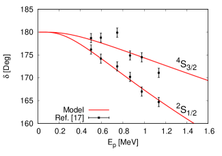
Figure 1: Phase shifts for the ${}^{2}S_{1/2}$ and the ${}^{4}S_{3/2}$ partial waves as function of the proton energy. The data are taken form Ref. [17]. The full red line are the calculated phase shifts with the potential parameters given in Table 3.

The $p-\,^{6}{\rm Li}$ potential of the form of Eq. (1) is used also in order to describe the ${}^{7}{\rm Be}$ nucleus. In this case we need to reproduce the binding energies of the two bound states, the ground state (GS) $J^{\pi}=3/2^{-}$ with $E=-5.6068$ MeV and the first excited state (FES) $J^{\pi}=1/2^{-}$ with $E=-5.1767$ MeV [23]. We fixed again the parameter $a_{0}$ as in Ref. [17], while in order to obtain $V_{0}$ we impose that the calculated binding energies reproduce the experimental ones up to the sixth digit. Moreover, we have evaluated also the asymptotic normalization coefficient (ANC), defined as

$${\rm{ANC}}=\frac{u_{LS}(r)}{\sqrt{2k}W_{L+1/2}(2kr,\eta)}\,,$$ (4)

where $u_{LS}(r)$ is the radial part of the wave function (see below), $r$ is the intercluster distance, $k=\sqrt{\frac{2\mu E}{\hbar^{2}}}$ with $\mu=\frac{m_{p}m_{{}^{6}{\rm Li}}}{m_{p}+m_{{}^{6}{\rm Li}}}$, $E$ the energy of the bound state, and $W_{L+1/2}(2kr,\eta)$ is the Whittaker function [24], with $\eta$ defined as

$$\eta=1.439975\times Z_{p}Z_{{}^{6}{\rm Li}}\frac{\mu}{2k\hbar^{2}}\,.$$ (5)

In Table 4 we report the values for $V_{0}$ and $a_{0}$, and the calculated value of the binding energies and ANCs for both the GS and FES. Note that, to our knowledge, there are no experimental data for the ANCs.

$J^{\pi}$	$V_{0}$ (MeV)	$a_{0}$ (fm-2)	$E$ (MeV)	ANC
$3/2^{-}$	254.6876510	0.25	-5.606800	2.654
$1/2^{-}$	252.7976803	0.25	-5.176700	2.528

Table 4: Values for the parameters of the Gaussian potential of Eq. (1) and the calculated binding energy and ANC for both the GS and the FES.

Having determined the ${}^{7}{\rm Be}$ and $p-\,^{6}{\rm Li}$ wave functions, we can proceed to evaluate the radiative capture cross section and angular distribution. Let us consider the generic reaction $A_{1}+A_{2}\rightarrow A_{3}+\gamma$. We write the scattering wave function as

$$\psi_{1,2}(\vec{r},p) = \frac{\sqrt{4\pi}}{p}\sum_{LSJJ_{z}}i^{L}\,\sqrt{2L+1}\,\langle J_{1}M_{1}J_{2}M_{2}|SJ_{z}\rangle$$ (6)

$$\langle SJ_{z}L0|JJ_{z}\rangle\,\psi_{1,2}^{LSJJ_{z}}(\vec{r},p)\,,$$

with

$$\psi_{1,2}^{LSJJ_{z}}(\vec{r},p)=R_{LSJ}(r,p)\,\Big{[}Y_{L}(\hat{r})\otimes\chi_{S}\Big{]}_{JJ_{z}}\,,$$ (7)

where $p$ is the relative momentum of the two particles, $\vec{r}$ the intercluster distance, $L$, $S$ and $J$ the total orbital, spin and angular momentum of the two nuclei, with $J_{1},M_{1}$ and $J_{2},M_{2}$ being the total angular momenta and third components of the two nuclei. The function $R_{LSJ}(r,p)$ is the scattering wave function, that has been determined solving the two-body Schrödinger equation similarly to what done in Ref. [8]. For the bound states of the final nucleus $A_{3}$ we write the wave function as

$$\psi_{3}^{J_{3}M_{3}}(\vec{r})=u_{L_{3}S_{3}}(r)\,\Big{[}Y_{L_{3}}(\hat{r})\otimes\chi_{S_{3}}\Big{]}_{J_{3}M_{3}}\,,$$ (8)

where $\vec{r}$ is again the intercluster distance. The function $u_{L_{3}S_{3}}(r)$ has also been determined as explained above. The total cross section for a radiative capture in a bound state with total angular momentum $J_{3}$ is written as

$$\sigma_{J_{3}}(E) = \frac{32\pi^{2}}{(2J_{1}+1)(2J_{2}+1)}\,\frac{\alpha}{v_{\rm rel}}\,\frac{q}{1+q/m_{3}}$$ (9)

$$\qquad\times\sum_{\Lambda\geq 1}\sum_{LSJ}\Big{(}|E_{\Lambda}^{LSJ,J_{3}}|^{2}+|M_{\Lambda}^{LSJ,J_{3}}|^{2}\Big{)}\,,$$

where $\alpha=e^{2}/4\pi$, $v_{\rm rel}$ is the relative velocity of the two incoming particles, $q$ is the photon momentum and $m_{3}$ is the mass of $A_{3}$ nucleus. Finally, $T_{\Lambda}^{LSJ,J_{3}}$, with $T=E/M$, are the reduced matrix element of the electromagnetic operator and $\Lambda$ is the multipole order. Using the Wigner-Eckart theorem, they are defined as

$$T^{LSJ,J_{3}}_{\Lambda}=\langle\psi_{1,2}^{LSJJ_{z}}(\vec{r},p)|T_{\Lambda\lambda}|\psi_{3}^{J_{3}M_{3}}(\vec{r})\rangle\frac{\sqrt{2J_{3}+1}}{\langle J_{3}M_{3}\Lambda\lambda|JJ_{z}\rangle}\,,$$ (10)

where $\lambda=\pm 1$ is the photon polarization. In our calculation we include only the electric operator, which is typically larger than the magnetic one. Then, in the long-wavelength approximation [25], by using Eqs. (7) and (8), it results

$$E_{\Lambda}^{LSJ,J_{3}} = (-1)^{2J_{f}+\Lambda+L+S-J}\hat{J}\hat{J_{3}}\hat{L_{3}}\hat{\Lambda}\,\langle L_{3}0\Lambda 0|L0\rangle$$ (11)

$$\times\begin{Bmatrix}J&L&S\\ L_{3}&J_{3}&\Lambda\end{Bmatrix}\frac{Z_{e}^{(\Lambda)}}{(2\Lambda+1)!!}\sqrt{\frac{\Lambda+1}{\Lambda}}\frac{q^{\Lambda}}{\sqrt{4\pi}p}$$

$$\times\int_{0}^{\infty}dr\,r^{2}\,u_{L_{3}S_{3}}(r)r^{\Lambda}R_{LSJ}(r,p)\delta_{S,S_{3}}\,.$$

Here we have defined $\hat{x}=\sqrt{2x+1}$ and

$$Z_{e}^{(\Lambda)}=Z_{1}\left(\frac{m_{2}}{m_{1}+m_{2}}\right)^{\Lambda}+Z_{2}\left(-\frac{m_{1}}{m_{1}+m_{2}}\right)^{\Lambda}\,$$ (12)

is the effective charge, in which $Z_{1}(Z_{2})$ is the charge and $m_{1}(m_{2})$ is the mass of the $A_{1}(A_{2})$ nucleus. Given the radial wave functions $u_{L_{3}S_{3}}(r)$ and $R_{LSJ}(r,p)$, the one-dimensional integral of Eq. (11) is simple and performed with standard numerical techniques. The astrophysical $S$-factor is then defined as

$$S_{J_{3}}(E)=E\exp(2\pi\eta)\sigma_{J_{3}}(E)\,,$$ (13)

where $\sigma_{J_{3}}(E)$ is the total cross section of Eq. (9) and $\eta$ is defined in Eq. (5).

The other observable of interest is the photon angular distribution, which can be written as

$$\sigma_{J_{3}}(E,\theta)=\sigma_{0}(E)\sum_{k}a_{k}^{J_{3}}(E)P_{k}(\cos\theta)\,,$$ (14)

where $\sigma_{0}(E)$ is a kinematic factor defined as

$$\sigma_{0}(E)=\frac{16\pi^{2}}{(2J_{1}+1)(2J_{2}+1)}\frac{\alpha}{v_{\rm rel}}\frac{q}{1+q/m_{3}}\,,$$ (15)

and $P_{k}(\cos\theta)$ are the Legendre polynomials. The coefficients $a_{k}$ are given by

$$a_{k}^{J_{3}}(E) = \sum_{LL^{\prime}SJJ^{\prime}\Lambda\Lambda^{\prime}}(-)^{J+J^{\prime}+J_{3}+L^{\prime}+\Lambda+S+1}\,i^{L+L^{\prime}+\Lambda+\Lambda^{\prime}}$$ (16)

$$\times\hat{L}\hat{L^{\prime}}\hat{\Lambda}\hat{\Lambda^{\prime}}\hat{J}\hat{J^{\prime}}\,\langle L0L^{\prime}0|k0\rangle\begin{Bmatrix}L&L^{\prime}&k\\ J^{\prime}&J&S\end{Bmatrix}$$

$$\times\begin{Bmatrix}J^{\prime}&J&k\\ \Lambda&\Lambda^{\prime}&J_{3}\end{Bmatrix}\sum_{\lambda=\pm 1}\langle\Lambda^{\prime}-\lambda\Lambda\lambda|k0\rangle$$

$$\times\left(\lambda M_{\Lambda^{\prime}}^{L^{\prime}SJ^{\prime},J_{3}}+E_{\Lambda^{\prime}}^{L^{\prime}SJ^{\prime},J_{3}}\right)\left(\lambda M_{\Lambda}^{LSJ,J_{3}}+E_{\Lambda}^{LSJ,J_{3}}\right)\,.$$

The photon angular distribution can be casted in the final form

$$\sigma_{J_{3}}(E,\theta)=\sigma_{J_{3}}(E)\left(1+\sum_{k\geq 1}A^{J_{3}}_{k}(E)P_{k}(\cos\theta)\right)\,,$$ (17)

where $\sigma_{J_{3}}(E)$ is defined in Eq. (9), and $A^{J_{3}}_{k}(E)=a_{k}^{J_{3}}(E)/a_{0}^{J_{3}}(E)$.

3 Results

In this section we compare our theoretical predictions for the astrophysical $S$-factor and the angular distribution of the emitted photon with the available experimental data. In the last subsection, we also discuss the possibility of introducing in our model the resonance proposed in Ref. [13].

Before discussing the results, we note that in the $p-\,^{6}{\rm Li}$ reaction the open ${}^{3}{\rm He}-\,^{4}{\rm He}$ channel should in principle be included. However, we do not consider this channel in our work. This can be done because the experimental phase shifts of Ref. [17] used to fit our potential were obtained considering only the $p-\,^{6}{\rm Li}$ channel. Therefore the ${}^{3}{\rm He}-\,^{4}{\rm He}$ channel results to be hidden in the experimental phase shifts that we reproduce with our potential. On the other hand, for the ${}^{7}{\rm Be}$ bound states, the ${}^{3}{\rm He}-\,^{4}{\rm He}$ component needs to be considered, and this is done phenomenologically, introducing in our calculation the spectroscopic factors, as explained in the next subsection.

3.1 The Astrophysical $S$-factor

The main contribution to the radiative capture reaction ${}^{6}{\rm Li}(p,\gamma)^{7}{\rm Be}$ cross section (and therefore astrophysical $S$-factor) comes from the electric dipole ($E1$) transition. The structure of the electric operator in the long wavelength approximation implies a series of selection rules due to the presence of the Wigner-6j coefficient as shown in Eq. (11). Therefore, the only waves allowed by the $E1$ transition operator up to $L=2$ are ${}^{2}S_{1/2}$, ${}^{2}D_{3/2}$ and ${}^{2}D_{5/2}$ for the GS, and ${}^{2}S_{1/2}$ and ${}^{2}D_{3/2}$ for the FES. To evaluate the ${}^{2}D$ waves, we use the same potential used for the ${}^{2}S_{1/2}$ wave, but we have changed only the angular momentum $L$ in the Schrödinger equation and we have imposed that the waves ${}^{2}D_{3/2}$ and ${}^{2}D_{5/2}$ are identical in the radial part. From the calculation, it turns out that up to energies of about 400 keV, the contribution of the ${}^{2}D$ waves is very small. However, for higher values of the energy, this contribution becomes significant.

In Fig. 2 we compare our results for the astrophysical $S$-factor with the experimental data of Ref. [9] and [13]. The calculation is performed summing up the contributions to both the GS and the FES. Since the data of Ref. [13] are still under debate, in discussing the results of Fig. 2 we will consider only the data of Ref. [9]. By inspection of the figure, we can conclude that our calculated (bare) $S$-factor is systematically lower than the data. The reason can be simply traced back to the fact that in our model we do not take into account the internal structure of ${}^{6}{\rm Li}$ and ${}^{7}{\rm Be}$. In order to overcome this limitation, we introduce the spectroscopic factor $\cal{S}$, for both bound states of ${}^{7}{\rm Be}$, so that the total cross section can be rewritten as

$$\sigma(E)={\cal{S}}_{0}^{2}\sigma^{\rm{bare}}_{0}(E)+{\cal{S}}_{1}^{2}\sigma^{\rm{bare}}_{1}(E)\,.$$ (18)

Here $\sigma^{\rm{bare}}_{0}(E)\,(\sigma^{\rm{bare}}_{1}(E))$ and ${\cal{S}}_{0}({\cal{S}}_{1})$ are the calculated bare cross section and spectroscopic factor for the transition to the GS (FES) of ${}^{7}{\rm Be}$.

In order to determine the two spectroscopic factors ${\cal{S}}_{0}$ and ${\cal{S}}_{1}$, we proceed as follows: we notice that in Ref. [9] there are two sets of data, which corresponds to the radiative capture to GS and FES, and the total $S$-factor is given by multiplying the data for the relative branching ratio (BR). Therefore, we divide the two data sets for the corresponding BR and we fit the spectroscopic factors, calculating the $S$-factor for GS and FES captures separately. In such a way we are able to reproduce not only the total $S$-factor but also the experimental BR for the FES radiative capture of $\sim 39\%$ [9], defined as ${\cal{S}}_{1}^{2}\sigma^{\rm{bare}}_{1}(E)/\sigma(E)$. The values of the spectroscopic factors and the $\chi^{2}/$datum defined according to Eq. (3), using the data of Ref. [9], before ($\chi^{2}_{0}/$datum) and after ($\chi^{2}_{\cal S}/$datum) adding the spectroscopic factors are given in Table 5. From the values of the $\chi^{2}_{0}/$datum given in Table 5, it is possible to conclude that the description of the radiative capture reaction to the GS using the bare wave function is quite accurate, while this is not the case for the FES.

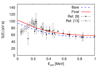
Figure 2: Total astrophysical $S$-factor for the ${}^{6}{\rm Li}(p,\gamma)^{7}{\rm Be}$ radiative capture reaction. The (blue) dashed line is the bare calculation, while the (red) full line is the obtained including the spectroscopic factors ${\cal{S}}_{0}$ and ${\cal S}_{1}$ of Table 5. The data are taken from Refs. [9] and [13].

$J^{\pi}$	${\cal S}$	$\chi_{0}^{2}/$datum	$\chi^{2}_{\cal{}_{S}}/$datum
$3/2^{-}$	1.003	0.064	0.064
$1/2^{-}$	1.131	2.096	0.219

Table 5: Spectroscopic factors ${\cal S}$ and $\chi^{2}/$datum obtained by fitting the data of Ref. [9], before ($\chi^{2}_{0}/$datum) and after ($\chi^{2}_{\cal S}/$datum) adding the spectroscopic factors themselves. With $J^{\pi}=3/2^{-}$ and $J^{\pi}=1/2^{-}$ we indicate the GS and FES of ${}^{7}{\rm Be}$.

In order to extrapolate the astrophysical $S$-factor at zero energy, we perform a polynomial fit of our calculated points up to second order, i.e. we rewrite the $S$-factor $S(E)$ in the energy range between $0$ and $300$ keV as

$$S(E)=S(0)+S_{1}(0)E+S_{2}(0)E^{2}\,.$$ (19)

In Table 6 we report the values obtained for $S(0)$, $S_{1}(0)$, and $S_{2}(0)$ in the cases of the GS, FES and the total GS+FES captures.

	GS	FES	GS+FES	Ref. [16]	Ref. [17]	Ref. [18]
$S(0)$ [eV b]	$\phantom{-}63.2$	$\phantom{-}40.7$	$\phantom{-}103.9$	$\phantom{-}98.5$	$\phantom{-}106$	$\phantom{-}108$
$S_{1}(0)$ [eV b/MeV]	$-63.9$	$-41.2$	$-105.1$	$-71.5$	$-215$	$-130$
$S_{2}(0)$ [eV b/MeV2]	$\phantom{-}27.3$	$\phantom{-}17.7$	$\phantom{-}45.0$	$\phantom{-}32.5$	$\phantom{-}312$	$\phantom{-}81.7$

Table 6: Expansion coefficients for the polynomial fit of the $S$-factor as defined in Eq. (19). For our work we report the expansion for the GS, the FES, and the sum of the two. For Refs. [16, 17, 18] we report the expansion obtained from the fit of digitalized curves of the total S-factor.

The results of the table can be compared with those obtained with other phenomenological models in Refs. [16, 17, 18]. In particular, we can conclude that our results for $S(0)$ is within $3\%$ compared to Refs. [16, 17, 18]. As regarding the shape of the $S$-factor, determined by $S_{1}(0)$ and $S_{2}(0)$, our results are quite in agreement with those of Ref. [16] and [18]. On the other hand, the results obtained in Ref. [17] with an approach similar to ours, give a higher value for $S_{1}(0)$ and $S_{2}(0)$. The origin of this discrepancy is still unknown. The results of Ref. [19], although obtained with a more sophisticated model than the one presented here, are consistent with ours, while those of Ref. [20] show a different energy dependence. All the theoretical calculations, except the studies of Refs. [11, 12], agree in a negative slope in the $S$-factor at low energies, and none of them predict a resonance structure, as suggested instead by the data of Ref. [13].

In order to estimate the theoretical uncertainty arising from a calculation performed in the phenomenological two-body cluster approach, we have reported in Fig. 3 within a (gray) band all the results available in the literature. As we can conclude by inspection of the figure, the theoretical error which can be estimated by the band is quite significant, but of the same order of the experimental errors on the data.

Figure 3: Comparison between our predictions (full red line) and the studies available in the literature. We show within a (gray) band the calculated astrophysical $S$-factors of Refs. [16, 17, 18], obtained with phenomenological potentials. For completeness we also report the results of Ref. [19] (blue dashed line) and of Ref. [20] (blue dot-dashed line).

If we take into account all the results obtained with the phenomenological potentials of Refs. [16, 17, 18] and the results of the present work, we obtain for the $S$-factor at zero energy the value

$$S(0)=(103.5\pm 4.5)\ {\rm eV\ b}\,.$$ (20)

We remark that also the value for $S(0)$ obtained in Ref. [21] is within this range.

3.2 Angular distribution of photons

We present in this section the photon angular distribution results obtained within the framework outlined in Sec. 2, and we compare our results with the data of Ref. [10]. This provides a further check on our model.

By using Eq. (17), we have found that the main contribution to the $A_{k}^{J_{3}}(E)$ coefficients comes from the interference of the $E1$ operator generated by the ${}^{2}S_{1/2}$ wave with the $E1$ operator generated by the ${}^{2}D$ waves and with the $E2$ operator generated by the ${}^{2}P$ waves. Note that for the ${}^{2}P$ and ${}^{2}D$ waves, we do not have a complete set of data for the phase shifts in all the possible total angular momentum $J^{\pi}$. Therefore we use the same radial function for the ${}^{2}D_{3/2}$ and ${}^{2}D_{5/2}$ waves, and also for the ${}^{2}P_{1/2}$ and ${}^{2}P_{3/2}$ waves. The relative phases for these waves, being arbitrary, are fixed in order to have the best description of the data of Ref. [10].

The results for the $A_{k}^{J_{3}}$ coefficients for various incident proton energies $(E_{p})$ are reported in Tables 7 and 8, where they are compared with the values fitted on the experimental data of Ref. [10].

$k\,(J_{3}=3/2)$	This work	Fit of Ref. [10]
$E_{p}=500$ keV
1	0.000	-
2	0.270	$0.299\pm 0.045$
3	0.000	-
$\chi^{2}/$datum	0.95	0.90
$E_{p}=800$ keV
1	0.000	-
2	0.375	$0.390\pm 0.031$
3	0.000	-
$\chi^{2}/$datum	0.79	1.17
$E_{p}=1000$ keV
1	0.000	-
2	0.422	$0.368\pm 0.036$
3	0.000	-
$\chi^{2}/$datum	1.61	1.21

Table 7: Values of the coefficients $A_{k}^{3/2}(E)$ for three proton energies compared with the fit to the data of Ref. [10]. The $\chi^{2}/$datum is also reported.

$k\,(J_{3}=1/2)$	This work	Fit of Ref. [10]
$E_{p}=500$ keV
1	0.214	$0.193\pm 0.055$
2	0.286	$0.159\pm 0.074$
3	0.043	-
$\chi^{2}/$datum	1.71	0.78
$E_{p}=800$ keV
1	0.263	$0.283\pm 0.042$
2	0.398	$0.257\pm 0.051$
3	0.085	-
$\chi^{2}/$datum	3.12	0.76
$E_{p}=1000$ keV
1	0.280	$0.205\pm 0.043$
2	0.448	$0.281\pm 0.054$
3	0.115	-
$\chi^{2}/$datum	6.10	1.67

Table 8: Same as Table 7, but for the coefficients $A_{k}^{1/2}(E)$.

In Figs. 4 and 5 we report the calculated angular distribution of the emitted photon for the capture to the GS and to the FES, respectively of $E_{p}=0.5$ MeV. The data of Ref. [10] are also shown.

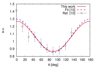
Figure 4: Photon angular distribution for the radiative capture to the GS for $E_{p}=0.5$ MeV. Our calculation (full red line) is compared to the fit (dashed blue line) and the data of Ref. [10].

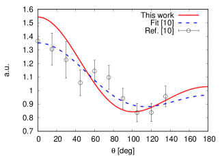
Figure 5: The same as Fig. 4 for the FES.

The theoretical values are in nice agreement with the fitted data for the GS. In particular, the $A_{1}^{3/2}$ coefficient, obtained using Eq. (16), results to be

$$A_{1}^{3/2}\propto E_{1}^{0\frac{1}{2}\frac{1}{2},\frac{3}{2}}\left(E_{2}^{1\frac{1}{2}\frac{1}{2},\frac{3}{2}}-E_{2}^{1\frac{1}{2}\frac{3}{2},\frac{3}{2}}\right)+\ldots\ ,$$ (21)

where the dots indicate the interference’s between the $E1$ generated by the $D$ waves, which give a negligible contribution. If now we suppose that $E_{2}^{1\frac{1}{2}\frac{1}{2},\frac{3}{2}}\simeq E_{2}^{1\frac{1}{2}\frac{3}{2},\frac{3}{2}}$, the value for $A_{1}^{3/2}$ goes to zero, explaining why we do not need this coefficient to reproduce the data. In our case the values of the coefficients $A_{1}^{3/2}$ are exactly zero because we use the same radial function for different $J^{\pi}$. The same happens also for $A_{3}^{3/2}$. As regarding to the capture to the FES, our calculation shows some disagreements compared to the values obtained by fit to the data of Ref. [10], although these are affected by significant uncertainties. In this case, in fact, there is no cancellation as in Eq. (21), and therefore the values of the coefficients $A_{k}^{1/2}$ are strongly dependent on the ${}^{2}P$ and ${}^{2}D$ waves, which are very uncertain. For this reason the disagreement with the data can be considered acceptable.

The photon angular distribution has a noticeable impact on the experimental measurements of the $S$-factor. Many experiments are done measuring the photon emitted at a fixed angle ($\theta$) respect to the beam axis. Therefore the measured cross section must be corrected by a factor related to the angular distribution. We take into account this effect writing the total cross section as

$$\sigma(E)=\frac{2\pi}{\phi_{2}-\phi_{1}}\,\,\frac{\sigma_{exp}(E;\theta_{1}\theta_{2};\phi_{1}\phi_{2})}{\int_{\theta_{1}}^{\theta_{2}}d\theta\,\sin\theta\,C(E,\theta)}\,,$$ (22)

where $\sigma_{exp}(E;\theta_{1}\theta_{2};\phi_{1}\phi_{2})$ is the measured cross section integrated over the solid angle covered by the detector and

$$C(E,\theta)=1+\sum_{k\geq 1}A_{k}(E)P_{k}(\cos\theta)\,.$$ (23)

In Eq. (22) we call with $\phi$ the other polar angle. Many experiments put the detector at $\theta\simeq 55^{\circ}$, since $P_{k}(\cos 55^{\circ})\simeq 0$ and therefore the contribution of $A_{2}(E)$ can be neglected. However, the contribution from the $A_{1}(E)$ coefficient can not be always neglected. Using our calculation, we can estimate the impact of the angular distribution of the photon to the measurement of the ${}^{6}{\rm Li}(p,\gamma)^{7}{\rm Be}$ reaction. In Fig. 6 we evaluated the coefficients $C(E,\theta=55^{\circ})$ for the capture to the GS and the FES, neglecting the physical dimension of the detector. By inspection of the figure we can conclude that the correction given by the photon angular distribution is negligible for capture in the GS. This can be traced back to the fact that the coefficient $A_{1}^{J_{3}}\simeq 0$. However, $A_{1}^{J_{3}}\simeq 6-9\%$ for the FES in the region of interest of the BBN. This can have consequences for the different experimental determinations, affecting their systematic error estimate.

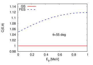
Figure 6: Correction coefficient $C(E,\theta)$ defined in Eq. (23) for the GS (full red line) and for the FES (dashed blue line) capture at $\theta=55^{\circ}$.

3.3 The “He”-resonance

In a recent work [13], He et al. considered the possibility of introducing a resonance-like structure in the ${}^{6}{\rm Li}(p,\gamma)^{7}{\rm Be}$ $S$-factor data at low energies, and they estimated the energy and width in the proton decay channel to be $E_{R}=195$ keV and $\Gamma_{p}=50$ keV, respectively. The total angular momentum of the resonance reported in Ref. [13] can be either $J^{\pi}=1/2^{+}$ or $J^{\pi}=3/2^{+}$. In this section we give for granted the existence of this resonance, and we explore the effects of introducing such a resonance structure in our model. The comparison with the available data will tell us whether this assumption is valid or not.

The first step of our study consists in constructing the nuclear potentials in such a way that we obtain $190$ keV $<E_{R}<$ $200$ keV and we reproduce the width of the resonance in the $S$-factor data. In a first calculation, we consider to introduce the resonance in the partial wave of spin 1/2. In particular we use the wave ${}^{2}S_{1/2}$ for $J^{\pi}=1/2^{+}$ and ${}^{2}D_{3/2}$ for $J^{\pi}=3/2^{+}$. In both the cases, we were not able to find parameters $V_{0}$ and $a_{0}$ (see Eq. (1)) that give a consistent description of all the available data. For the ${}^{2}S_{1/2}$ the introduction of such a resonance is completely inconsistent with the experimental phase shifts. For the ${}^{2}D_{3/2}$ we do not have experimental constrains on the experimental phase shifts, but we were not able to obtain the strength of the resonance as given in the data of Ref. [13]. The best result obtained adding the resonance in the ${}^{2}D_{3/2}$ wave is given in Fig. 7.

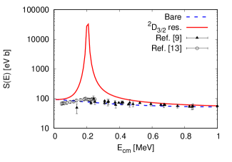
Figure 7: Bare astrophysical $S$-factor (blue dot-dashed line) to which it is summed a resonance structure in the ${}^{2}D_{3/2}$ wave (full red line). See text for more details.

In a second calculation, we considered the GS of ${}^{7}{\rm Be}$ to be a mixed state of spin $1/2$ and $3/2$. In this way the $E1$ operator can couple the scattering wave ${}^{4}S_{3/2}$ to the ${}^{4}P_{3/2}$ component of the GS. Therefore, we can introduce the $J^{\pi}=3/2^{+}$ resonance in the ${}^{4}S_{3/2}$ partial wave. In this calculation, we use the ${}^{2}P_{3/2}$ radial wave function for the ${}^{4}P_{3/2}$ component of the GS. We select as potential parameters for the ${}^{4}S_{3/2}$ component $V_{0}=438.7$ MeV and $a_{0}=0.2$ fm^-2. With this potential we get a resonance energy of $E_{R}=197$ keV and a width of the resonance $\Gamma\sim 15$ keV. The difference in the width compared to the value reported by Ref. [13] is mainly due to the fact we do not include interferences with the ${}^{3}{\rm He}-\,^{4}{\rm He}$ channel. Then we rewrite the total cross section as

$$\sigma(E)={\cal{S}}_{0}^{2}\sigma^{\rm{bare}}_{0}(E)+{\cal{S}}^{2}_{1}\sigma^{\rm{bare}}_{1}(E)+{\cal{S}}_{\rm{res}}^{2}\sigma^{\rm{bare}}_{\rm{res}}(E)\,,$$ (24)

where ${\cal{S}}_{\rm{res}}$ is the spectroscopic factor of the ${}^{4}P_{3/2}$ wave component in the GS and $\sigma^{\rm{bare}}_{\rm{res}}$ is the calculated capture reaction cross section in the resonance wave. The result obtained imposing ${\cal{S}}_{0}={\cal{S}}_{1}\sim 1$ and ${\cal{S}}_{\rm{res}}\sim 0.011$ is in good agreement with both the data set of Refs. [9] and [13] and it is shown in Fig. 8. The small value of ${\cal{S}}_{\rm{res}}$ reflects the small percentage of spin 3/2 component in the ${}^{7}{\rm Be}$ GS.

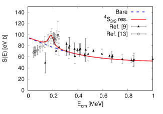
Figure 8: Bare astrophysical $S$-factor (blue dot-dashed line) to which it is summed a resonance structure in the ${}^{4}S_{3/2}$ wave (full red line). See text for more details.

To be noticed that our results are also consistent with the R-matrix fit reported in Ref. [13]. However, using the potential model which describes the resonance in the $S$-factor data, we were not able to reproduce the ${}^{4}S_{3/2}$ elastic phase shifts data. In fact, as shown in Fig. 9, the ${}^{4}S_{3/2}$ phase shift is badly underpredicted.

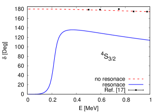
Figure 9: Elastic scattering phase shifts for the ${}^{4}S_{3/2}$ wave calculated in the case of resonance (blue full line) and no resonance (red dashed line), are compared with the data of Ref. [17].

Therefore we can conclude that by including the resonance structure in the ${}^{4}S_{3/2}$ wave, we obtain a nice description of the $S$-factor data, but we destroy the agreement between theory and experiment for the elastic phase shifts. This put under question the real existence of the resonance structure proposed in Ref. [13].

4 Summary and Conclusions

We have evaluated the astrophysical $S$-factor of the ${}^{6}{\rm Li}(p,\gamma)^{7}{\rm Be}$ radiative capture reaction using a two-body cluster approach. The intercluster potential parameters are fitted to reproduce the bound state properties of ${}^{7}{\rm Be}$ and the scattering phase shifts for all the partial waves of interest. The wave functions are calculated solving the Schrödinger equation with the Numerov method.

The theoretical $S$-factor underestimates, although not dramatically, the experimental values. This is not surprising, since we have neglected in this first step the internal structure of the involved nuclei. When we introduce a spectroscopic factor, which takes care of this, we obtain a nice agreement with the data. Furthermore, we have reviewed the phenomenological calculations present in literature, and this has allowed us to estimate the theoretical error on the $S$-factor calculated within this two-body approach.

We have also studied the photon angular distribution. Comparing our calculations with the available data, we obtain a good description of the angular distribution for the capture to the GS of ${}^{7}{\rm Be}$. For the capture to the FES, the description is less accurate, and this can be traced back to the poor knowledge of the $P$ and $D$ waves phase shifts. Furthermore, we have used our calculation of the photon angular distribution to study the effect on the experimental error budget for those experiments which measure the ${}^{6}{\rm Li}(p,\gamma)^{7}{\rm Be}$ cross section using a fixed angle apparatus.

Finally, we have introduced in our study the resonance-like structure proposed in Ref. [13]. If the resonance is introduced in the ${}^{2}S_{1/2}$ or in the ${}^{2}D_{3/2}$ waves, we obtain results completely inconsistent with the phase shifts and S-factor data. When the resonance is introduced in the ${}^{4}S_{3/2}$ wave, a nice description of the $S$-factor data is achieved. However, we are not able to reproduce consistently the ${}^{4}S_{3/2}$ elastic scattering phase shifts. We can conclude therefore that the presence of a resonant structure cannot be accepted in our theoretical framework.

References

- [1] M. Asplund et al., Astrophys. J. 644, 229 (2006).
- [2] R. Cayrel et al., Astron. Astrophys. 473, L37 (2007).
- [3] A.E.G. Perez, W. Aoki, S. Inoue, S.G. Ryan, T.K. Suzuki, and M. Chiba, Astron. Astrophys. 504, 213 (2009).
- [4] M. Steffen, R. Cayrel, P. Bonifacio, H.G. Ludwig, and E. Caffau, IAU Symposium 265, 2324 (2010).
- [5] K. Lind, J. Melendez, M. Asplund, R. Collet, and Z. Magic, Astron. Astrophys. 544, A96 (2013).
- [6] M. Kusukabe et al., Phys. Rev. D 74, 023526 (2006).
- [7] S. Bashkin and R. R. Carlson, Phys. Rev. Lett. 97, 5 (1995).
- [8] A. Grassi, G. Mangano, L.E. Marcucci, and O. Pisanti, Phys. Rev. C 96, 045807 (2017).
- [9] Z.E. Switkowski et al., Nucl. Phys. A 331, 50 (1979).
- [10] C.I. Tingwell, J. D. King and D.G. Sargood, Aust. J. Phys. 40, 319 (1987).
- [11] F.E. Cecil et al., Nucl. Phys. A 539, 75 (1992).
- [12] R.M. Prior et al., Phys. Rev. C 70, 055801 (2004).
- [13] J.J. He et al., Phys. Lett. B 725, 287 (2013).
- [14] S.B. Igamov et al., Bullettin NNC RK (2016).
- [15] Z.-H. Li et al., arXiv:1803.10946 (2018).
- [16] J.T. Huang, C.A. Bertulani, and V. Guimaraes, At. Data Nucl. Data Tables 96, 824 (2010).
- [17] S.B. Dubovichenko et al., Phys. Atom. Nucl. 74, 1013 (2011).
- [18] F.C. Barker, Aust. J. Phys. 33, 159 (1980).
- [19] K. Arai, D. Baye, and P. Descouvemont, Nucl. Phys. A 699, 963 (2002).
- [20] G.X. Dong et al., J. Phys. G: Nucl. Part. Phys. 44, 045201 (2017).
- [21] P. Descuvemont and D. Baye, Rep. Prog. Phys. 73, 036301 (2010).
- [22] M.J.D. Powell, Acta Numerica 7, 287 (1998).
- [23] D.R. Tilley et al., Nucl. Phys. A 708, 3 (2002).
- [24] M. Abramowitz and I. A. Stegun, Handbook of Mathematical Functions with Formulas, Graphs, and Mathematical Tables, (Dover, New York, 1965).
- [25] J.D. Walecka, Theoretical Nuclear and Subnuclear Physics, (Oxford University Press, New York Oxford, 1995).