Robot Co-design: Beyond the Monotone Case

Abstract

Recent advances in 3D printing and manufacturing of miniaturized robotic hardware and computing are paving the way to build inexpensive and disposable robots. This will have a large impact on several applications including scientific discovery (e.g., hurricane monitoring), search-and-rescue (e.g., operation in confined spaces), and entertainment (e.g., nano drones). The need for inexpensive and task-specific robots clashes with the current practice, where human experts are in charge of designing hardware and software aspects of the robotic platform. This makes the robot design process expensive and time consuming, and ultimately unsuitable for small-volumes low-cost applications. This paper considers the computational robot co-design problem, which aims to create an automatic algorithm that selects the best robotic modules (sensing, actuation, computing) in order to maximize the performance on a task, while satisfying given specifications (e.g., maximum cost of the resulting design). We propose a binary optimization formulation of the co-design problem and show that such formulation generalizes previous work based on strong modeling assumptions. We show that the proposed formulation can solve relatively large co-design problems in seconds and with minimal human intervention. We demonstrate the proposed approach in two applications: the co-design of an autonomous drone racing platform and the co-design of a multi-robot system.

I Introduction

Recent advances in sensor design and rapid prototyping are enabling the manufacturing of low-cost robots with advanced sensing and perception capabilities. For instance, one can implement high-precision visual-inertial navigation with inexpensive camera and MEMS inertial measurement units [1]. Similarly, modern embedded CPU-GPU [2] offer high-performance computing in a compact form-factor and at a relatively affordable cost. These trends, together with the availability of low-cost micro-motors are enabling fast and cheap production of robotic platforms. In these cases, the most expensive resource becomes the effort of the expert human designers who are in charge of designing all the aspects of the robotic platform, including hardware and software. While this solution is still acceptable in the case where low-cost robots must be produced in volumes (e.g., vacuum cleaning robots), it may not be desirable when only few robots need to be deployed. Consider, for instance, the design of a drone for hurricane monitoring [3]: the drone must be disposable, hence inexpensive, and it is not typically produced in volumes. In other contexts, one may need to devise a design quickly, in order to create a robot to be deployed in a time-sensitive mission. For instance, one may need to design a search-and-rescue robot tailored to a specific mission (e.g., search for survivors in a narrow cave with a given size of the entry point). Finally, human design does not necessarily lead to optimal solutions. Designers typically consider different robotics modules in isolation in order to tame the design complexity, and such decoupling usually leads to suboptimal performance.

These reasons motivate us to investigate computational robot co-design, which aims to create an automatic algorithm that selects the best robotic modules (sensing, actuation, computing) in order to maximize the performance on a task, while satisfying given specifications (e.g., maximum cost of the resulting design). Here the term “computational” refers to the fact that the design techniques can be implemented on a machine, and require minimal human intervention. Moreover, the term “co-design” refers to the attempt to consider the robotic system as a whole, rather than (sub-optimally) decoupling the design of each module.

Related Work. The problem of co-design in robotics touches a wide span of research topics. In the most general sense, it can be considered as the problem of designing both the mind (software) and the body (hardware) of the robot at the same time. A few seminal works tackle this problem from an evolutionary standpoint [4, 5, 6], with approaches that aim to either optimize specific behaviors (e.g., walking) or to explore catalogs of possible solutions to a general problem (e.g., locomotion). While related to the problem of computational co-design as discussed above, these approaches typically abstract away several practical aspects of hardware design, such as power consumption and material selection.

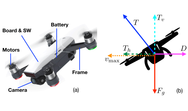
Figure 1: (a) We apply the proposed co-design framework to the design of the modules (motors, frame, computing, camera, battery pack) of an autonomous racing drone, (ii) Force diagram during forward motion (side view).

At the opposite side of the spectrum, a large body of work on software/hardware design exists in the embedded systems community, e.g. FPGA and ASIC design [1]. In this domain, the focus is on the synthesis of practical solutions that explicitly consider low-level aspects such as power optimization and real-time scheduling in electronic devices. Since Chinook [7], a highly influential early approach, the field of software/hardware co-design has flourished, reaching relevant applications in safety-critical fields such as the aerospace [8] and automotive industry. The inception of domain-specific languages such as the Architecture Analysis and Design Language (AADL) [9] has enabled a systems-of-systems approach in which co-design can be coupled with a wide array of tools for property verification, both at the software and hardware level. These tools, however, are thought to support human design.

The field of modular robotics attempts to bridge low-level embedded system design with high-level functionality specifications. In modular robotics, the challenge is to create a diverse set of composable, programmable modules that can be used to form robots with different capabilities. The recent, rapid development of 3D printing is offering increasingly powerful tools to streamline the automatic design of robotic platforms, and will arguably foster the development of modular robotics. In a seminal paper, Mehta et al. [10] demonstrate the feasibility of a procedure that takes a high-level human-defined specification of a robot and outputs the 3D description files of the components, along with instructions to assemble the robot, manufacture the electronics, and automatically generate the control firmware. To the best of our knowledge, no work exists in the automatic generation of specifications that can be input to this system.

A core issue in computational co-design is the conception of a suitable formalism to express the design problem. Ideally, an effective formalism for automatic design should combine adequate granularity along with guarantees of correctness. Evolutionary methods [4, 5, 6] combine a low-level parametric representation, such as rigid bodies connected by joints or voxel-based artifacts, with neural network-based control. The main issue of this representation is the amount of detail involved in the optimization process, which limits scalability, and the absence of correctness guarantees. Other formalisms closer to the human design process, such as the one from Mehta et al. [10] and AADL [9], achieve expressive power by naturally incorporating modularity. Both languages represent a co-design problem as a tree composed of heterogenous nodes which represent hardware and software aspects of a robot. AADL, in particular, offers a set of tools specifically designed for early analysis of candidate solutions, but without support for automatic exploration of the solution space. Correct-by-design compositional approaches have also been the focus of recent studies in control theory. For instance, Hussien et al. [11] proposed an automatic method to decompose a large control problem into a cascade of simpler problem, under the assumption that the latter are feedback linearizable, while Kim et al. [12] devised a method to arbitrarily construct system abstractions from simpler, well-posed components. Lastly, Censi [13, 14] proposed a powerful co-design approach that enables the automatic generation of solutions from a specification that includes recursive constraints. Censi’s approach assumes that a monotone mapping between resources and performance exists, thus casting computational co-design as a fixed-point problem in the solution space.

Contribution. This paper builds on recent work by Censi [13, 14] and pushes the boundary of computational co-design by relaxing its monotonicity assumption. Monotonicity implies that investing more resources leads to an increase in the performance. However, it is easy to find interesting examples for which this property does not hold. For instance, in the design if a drone frame, the fact that we increase the size of the frame (resource) does not imply that the drone will fly faster (performance). Similarly, in a collaborative transportation problem, deploying a larger number of robots (resources) does not necessarily lead to an increase in the overall performance of the system [15].

This paper presents a more general computational co-design approach. Our problem formulation is presented in Sec. II, where we discuss the characterization of the design space and classify the design specifications in terms of system-level performance, system-level constraints, and intrinsic constraints. Sec. II-C rephrases the resulting co-design problem in terms of a binary optimization problem, where each binary variable indicates whether a given component is chosen as part of the design or not. Sec. III discusses in which case we can expect to be able to solve the binary optimization problem using off-the-shelf optimization tools; in general, binary optimization is intractable, but there exist several algorithms and implementations that are able to solve moderate-sized problems efficiently as long as some property (e.g., linearity) holds. We show that our approach allows recasting several functions that are nonlinear in the properties (or features) of the robotic modules as linear functions. The proposed optimization framework also makes it possible to model other constraints found in practice, such as compatibility constraints (e.g., we cannot use a LIDAR-based algorithm to process data from a monocular camera), which was beyond reach for existing methods [13].

We conclude the paper by presenting two applications of the proposed co-design approach to the design of an autonomous drone racing platform and a multi-robot system. These examples are presented in Sec. IV. Drone design is an interesting topic per se, and has already received attention in the literature [16, 1], which however still lacks a computational design approach. New and untapped challenges arise in the co-design of multi-robot systems. We are not aware of approaches that specifically tackle this problem; however, a vast literature exist on the automatic generation of control systems for robots swarms, including evolutionary methods [17] and automatic generation of composable control structures [18].

II General Robot Co-design

The co-design problem consists in jointly designing robot software and hardware components to maximize task-dependent performance metrics (e.g., endurance, agility, payload) subject to constraints on the available resources (e.g., cost). The complexity of the problems stems from the fact that a robotic system involves an intertwining of modules. Each module contributes to the overall performance of the system while potentially consuming resources. In this paper, we consider the realistic case in which we have to choose each module (e.g., motor, embedded computer, camera) in the robotic system from a given catalog, and we formulate the co-design as the combinatorial selection of modules that maximize performance while satisfying given system-level and module-level constraints. In Sec. II-A we introduce our abstraction of the modules forming the overall robotic system. In Sec. II-B we describe the interactions among the modules and how they contribute to the overall system performance and resource utilization. In Sec. II-C we state the co-design problem as a binary optimization problem.

II-A Modules, Catalogs, Features

We consider the case in which the robotic system comprises a given set of modules ${\cal M}$. The modules may include, for instance, the actuators, the sensors, the computational board, the perception algorithms, the control algorithms, the planning algorithms, etc. For each module $i\in{\cal M}$, we have a catalog ${\cal C}_{i}$ of potential choices: for instance, we can purchase different motor models, or we can utilize different approaches and implementations of a planning algorithm.

Design vector. The goal of the co-design is to select an element $j\in{\cal C}_{i}$ (catalog for module $i$), for each module $i\in{\cal M}$. We can represent this selection using a binary vector ${\bm{x}}_{i}$ for each module, where the $j$-th entry of ${\bm{x}}_{i}$ is 1 if we select the $j$-th element in the catalog ${\cal C}_{i}$ or zero otherwise. Clearly, ${\bm{x}}_{i}\in\{0,1\}^{|{\cal C}_{i}|}$, where $|{\cal C}_{i}|$ is the cardinality (number of elements) of the catalog. Therefore, the design is fully specified by the design vector ${\bm{x}}$ obtained by stacking ${\bm{x}}_{i}$ for each $i\in{\cal M}$. The design vector has size $N\doteq\sum_{i\in{\cal M}}|{\cal C}_{i}|$, which we refer to as the dimension of the design space.

Feature matrix. Each module has a number of features describing the technical specifications of the module. For example, the features of a motor may include the cost, torque, weight, maximum speed, power consumption, size of the motor, among other technical data. In general, the features are a list of properties one would find in the datasheet of a component. Similarly, for an algorithm, the set of features may include information about the expected performance and computational cost of the algorithm.

Clearly, each element in the catalog of module $i$ (e.g., different motor models) will have different values of each feature. We can thus succinctly describe the list of features for each element in the catalog of module $i$ as a feature matrix ${\bm{F}}_{i}$, where each row correspond to a given feature, and different columns correspond to different elements in the catalog. For instance, in a toy problem, we can have the following feature matrix for the motor module:

$${\bm{F}}_{\text{m}}=\left[\begin{array}[]{ccc}W^{(1)}&W^{(2)}&W^{(3)}\\ V^{(1)}&V^{(2)}&V^{(3)}\\ A^{(1)}&A^{(2)}&A^{(3)}\\ C^{(1)}&C^{(2)}&C^{(3)}\\ T^{(1)}&T^{(2)}&T^{(3)}\end{array}\right]\begin{array}[]{l}\leftarrow\text{weight}\\ \leftarrow\text{voltage}\\ \leftarrow\text{current}\\ \leftarrow\text{cost}\\ \leftarrow\text{torque}\end{array}$$ (11)

where the $j$-th column describes the features of the $j$ element in the motor catalog. In practice, the values in the matrix are known from datasheet or from prior experiments.

Remark 1 (Beyond monotonicity)

A way to relate our approach (describing modules via catalogs and feature matrices) to the one of Censi [13] is as follows. Censi splits what we call features into resources and functionalities (imagine for instance, that the first $n_{r}$ rows or (11) are labeled as “resources” and the last $n_{p}$ as “functionalities”). Then, Censi assumes that the columns of (11) satisfy the monotonicity property, i.e., choices of components (columns) leading to better functionalities require more resources. This is not necessarily true in practice: if we design a drone system, choosing a larger frame (i.e., consuming more resources) does not necessarily imply that our drone will fly faster (i.e., better functionality). We go beyond [13] with two main innovations. First, the entries in our feature matrix (11) are completely arbitrary, hence relaxing the monotonicity assumption. We will further highlight the importance of relaxing monotonicity for multi-robot design in Sec. IV-B. Second, while resources and functionalities of each module may be problem-dependent, feature matrices are design-agnostic, as discussed in Remark 2 below.

Remark 2 (Feature matrices are design-agnostic)

The notion of “module” and “feature matrix” are agnostic of the co-design problem, which is only defined in Sec. II-C. Indeed, the notion of “features” is general—the same modules can be used in any co-design problem involving that module. This is in sharp contrast with [13], where the definition of “resources” and “functionalities” (or “performance”) for each module depends on the interactions between modules, hence it is problem-dependent. For instance: Fig. 21 in [13] classifies the battery capacity as a performance metric, but in other problems the battery capacity can be a resource. Our choice to create an intermediate abstraction, the feature matrix, resolves this dependence, enabling re-usability of modules across problems.

II-B Design Specifications: Performance and Constraints

In a robotic system, the different modules interact to contribute to the overall performance of the system and potentially consume resources. In particular, both the overall system as well as each module require a minimum amount of resources to operate properly, thus imposing constraints on the design.

In this context, we distinguish three main design specifications: system-level performance, system-level constraints, and module-level constraints. Intuitively, system-level performance defines a set of metrics the co-design has to maximize, while system-level (resp. module-level) constraints specify a set of constraints that need to be satisfied for the overall system (resp. each module) to operate correctly. These design specifications, which we discuss in more detail below, together with the catalogs of the modules we want to design, fully specify the co-design problem (Section II-C).

Explicit specifications: system-level performance and constraints. As an input to the co-design process, the user provides a set of performance metrics the design must maximize, as well as a set of constraints the overall system must satisfy. These specifications, which we refer to as explicit specifications, are at the system level, in the sense that they describe the task that the system must perform.

System-level Performance. The system-level performance is a vector-value function of a choice of components. Recalling that a design is fully characterized by the design vector ${\bm{x}}$, the system-level performance is a function:

$$\text{SP}({\bm{x}}):\{0,1\}^{N}\mapsto{{\mathbb{R}}^{N_{p}}},$$ (12)

where $N$ is the dimension of the design space and $N_{p}$ is the number of performance metrics the user specifies. To clarify (12), let us consider a simple example, in which the design must maximize the torque of the wheel motors of an autonomous race car. In this case, the system-level performance is described by:

$$\text{SP}({\bm{x}})=4\;[{\bm{F}}_{\text{m}}]_{T}\;{\bm{x}}_{\text{m}}$$ (13)

In (13), ${\bm{F}}_{\text{m}}$ is the motor feature matrix in (11), ${\bm{x}}_{\text{m}}$ is the design vector for the motor module, and $[{\bm{F}}_{\text{m}}]_{T}$ extracts the row of ${\bm{F}}_{\text{m}}$ corresponding to the motor torque. The factor “4” captures the fact that, for simplicity, we assumed four wheels mounting identical motors. We remark that the (linear) operator $[\cdot]_{T}$ selects the row corresponding to a specific feature from the feature matrix, while the multiplication by ${\bm{x}}_{\text{m}}$ has the effect of selecting a single column (i.e., choosing a motor model) from ${\bm{F}}_{\text{m}}$, due to the fact that ${\bm{x}}_{\text{m}}$ has a single non-zero element.

System-level Constraints. The system-level constraints are (scalar) equality or inequality constraints, describing hard requirements on the desired behavior of the system or constraints on the resources that can be used for the design. We express system-level constraints involving the design vector ${\bm{x}}$:

$$\text{SC}({\bm{x}})_{k}\leq 0 \text{for }k\in{\cal SC}_{\leq}$$ (14)

$$\text{SC}({\bm{x}})_{k^{\prime}}=0 \text{for }k^{\prime}\in{\cal SC}_{=}$$ (15)

where ${\cal SC}_{\leq}$ and ${\cal SC}_{=}$ are the sets of inequality and equality system-level constraints, respectively. For instance, we can have an upper bound on the overall cost of the design:

$$\sum_{i\in{\cal M}}\;[{\bm{F}}_{i}]_{C}\;{\bm{x}}_{i}\leq\text{budget}\Rightarrow\text{SC}({\bm{x}})_{k}=\sum_{i\in{\cal M}}\;[{\bm{F}}_{i}]_{C}\;{\bm{x}}_{i}-\text{budget}$$ (16)

where, as before, the linear operator $[\cdot]_{C}$ extracts the cost from the feature matrix of each module $i$. Note that the “budget” must be provided by the user and it is specific to the design instance, hence (16) is a system-level constraint.

An example of system-level equality constraint is the case in which the user wants to consider only a subset of elements in the catalog (e.g., within a catalog of motors, only two motors are available in-house). For instance, for the choice of module $i$ to be restricted to the subset ${\cal S}_{i}\subset{\cal C}_{i}$, the user can add the following system-level equality constraint:

$$\sum_{j\in{\cal S}_{i}}[{\bm{x}}_{i}]_{j}=1\quad\Rightarrow\quad\text{SC}({\bm{x}})_{k^{\prime}}=\sum_{j\in{\cal S}_{i}}[{\bm{x}}_{i}]_{j}-1$$ (17)

where again $[{\bm{x}}_{i}]_{j}$ selects the $j$-th element of ${\bm{x}}_{i}$; the constraint (17) enforces one element in ${\cal S}_{i}$ to be chosen, due to the binary nature of the vector ${\bm{x}}_{i}$.

Implicit specifications: module-level constraints. The user must provide explicit specifications to describe what the robotic system is required to do within which operational constraints. On the other hand, implicit specifications are transparent (or uninteresting) to the user and are only needed to guarantee that each module has sufficient resources to function as expected.

Similarly to the system-level performance, we express module-level (implicit) constraints as inequality or equality constraints involving the design vector ${\bm{x}}$:

$$\text{IC}({\bm{x}})_{k}\leq 0 \text{for }k\in{\cal IC}_{\leq}$$ (18)

$$\text{IC}({\bm{x}})_{k^{\prime}}=0 \text{for }k^{\prime}\in{\cal IC}_{=}$$ (19)

where ${\cal IC}_{\leq}$ and ${\cal IC}_{=}$ are the sets of inequality and equality module-level constraints, respectively. While the mathematical nature of the system-level and module-level constraints is similar, we believe it makes sense to distinguish them, since the user has control over system-level constraints (e.g., to increase the design budget in (16)), while he/she typically does not have control over the implicit constraints.

For instance, the user cannot change the fact that, for the system to function properly, the onboard battery “b” has to provide enough power for all the active modules (say, motors “m”, sensors “s”, and computing “c”), which indeed translates into an implicit inequality constraint:

$$\begin{array}[]{lll}A_{\text{b}}V_{\text{b}}\geq A_{\text{m}}V_{\text{m}}+A_{\text{s}}V_{\text{s}}+A_{\text{c}}V_{\text{c}}\quad\Rightarrow\!\!\!\!\\ \quad\text{IC}({\bm{x}})_{k}=\!\!\!\!\displaystyle\sum_{i=\{\text{m},\text{s},\text{c}\}}\!\!\!\!([{\bm{F}}_{i}]_{A}{\bm{x}}_{i})([{\bm{F}}_{i}]_{V}{\bm{x}}_{i})-([{\bm{F}}_{b}]_{A}{\bm{x}}_{b})([{\bm{F}}_{\text{b}}]_{V}{\bm{x}}_{\text{b}})\!\!\!\!\end{array}$$ (20)

where $A_{i}$ and $V_{i}$ are the current and voltage at module $i$, and ${\bm{F}}_{i}$ is again the feature matrix for module $i$.

Implicit constraints are also useful to model compatibility constraints, which, again, the user is not typically free to alter. For instance, we may want to model the fact that we cannot run a certain algorithm (e.g., designed for FPGA) on a certain hardware (e.g., CPU), or we cannot use a LIDAR-based signal processing front-end to process data from a monocular camera. Compatibility constraints can be expressed as follows, for a pair of modules “a” and “b”:

$$[{\bm{x}}_{a}]_{j}\leq\sum_{j^{\prime}\in{\cal S}_{j}}[{\bm{x}}_{b}]_{j^{\prime}}$$ (compatibility)

$$\;[{\bm{x}}_{a}]_{j}\leq 1-\sum_{j^{\prime}\in{\cal S}_{j}}[{\bm{x}}_{b}]_{j^{\prime}}$$ (incompatibility) (21)

The first inequality in (21) imposes that, when the $j$-th element in the catalog of module “a” is selected, we can only choose the module $b$ from the subset ${\cal S}_{j}$ (subset of compatible modules in the catalog of $b$). The second inequality in (21) imposes that, when the $j$-th element in the catalog of module “a” is selected, then we cannot choose the module $b$ from the subset ${\cal S}_{j}$ (subset of incompatible modules in the catalog).

II-C Co-design

The co-design problem can be now stated as follows.

Definition 3 (Robot Co-design)

Given the catalogs (and the corresponding feature matrices ${\bm{F}}_{i}$) for each module $i\in{\cal M}$ to be designed, given the system-level performance function $\text{SP}({\bm{x}})$ and the set of system-level inequality and equality constraints (${\cal SC}_{\leq},{\cal SC}_{=}$), as well as the set of module-level inequality and equality constraints (${\cal IC}_{\leq},{\cal IC}_{=}$), robot co-design searches for the choice of modules ${\cal M}$ that maximizes the system-level performance, while satisfying the constraints:

$$\max_{{\bm{x}}\in{\cal X}} \text{SP}({\bm{x}})$$ (22)

subject to $$\text{SC}({\bm{x}})_{k}\leq 0 \text{for }k\in{\cal SC}_{\leq}$$

$$\text{SC}({\bm{x}})_{k^{\prime}}=0 \text{for }k^{\prime}\in{\cal SC}_{=}$$

$$\text{IC}({\bm{x}})_{k}\leq 0 \text{for }k\in{\cal IC}_{\leq}$$

$$\text{IC}({\bm{x}})_{k^{\prime}}=0 \text{for }k^{\prime}\in{\cal IC}_{=}$$

where ${\cal X}$ is the set of binary vectors that correspond to unique choices of each module (mathematically: ${\cal X}\doteq\{\{0,1\}^{N}\;{:}\;\sum_{j=1}^{|{\cal C}_{i}|}[{\bm{x}}_{i}]_{j}=1\text{ for each module }i\in{\cal M}\}$).

Problem (22) is a binary optimization problem, since the vector-variable ${\bm{x}}$ has binary entries. The formulation does not take any assumption on the nature of the functions involved in the objective function and the constraints. Our formulation is this general and it does not assume monotonicity: indeed, by introducing the notion of “feature matrix”, we circumvented the problem of reasoning in terms of resources and functionality of each module. As we will see, this framework allows one to solve non-monotonic problems (see Sec. IV).

Remark 4 (Total Order)

In general, the optimization problem (22) is a multi-objective maximization, since the objective is vector-valued. While a major concern in [13] was how to deal with partially ordered sets (e.g., vectors), here we take a more pragmatic approach. In the formulation (22) we assume a total order for the vector in the objective, while we restricted the constraints to be scalar equalities and inequalities, hence working on the totally ordered set of reals. In particular, we use the lexicographical order to enforce a total order on a vector space of performance vectors. In the lexicographical order two vectors ${\bm{y}}=[y_{1}\;y_{2}\;\ldots\;y_{n}]$ and ${\bm{z}}=[z_{1}\;z_{2}\;\ldots\;z_{n}]$ satisfy ${\bm{y}}\leq{\bm{z}}$ if an only if $y_{1}\leq z_{1}$, or $y_{1}=z_{1}$ and $y_{2}\leq z_{2}$, or $y_{1}=z_{1}$, $y_{2}=z_{2}$ and $y_{3}\leq z_{3}$ etc. This order implies that the entries of the vector are sorted by “importance”. For instance, if we minimize a performance vector that includes $[\text{cost},\;\text{size}]$, then we search for the design that minimizes cost, and if two designs have the same cost, we prefer the design with smaller size. Note that we can also use the lexicographical order to generalize the constraints to be vector-valued functions.

III Linear Co-design Solvers

We now discuss several cases in which we can expect to solve Problem (22) in reasonable time using off-the-shelf optimization tools. While Problem (22) is fairly general (we did not take any assumptions on the functions involved in the objective and the constraints), we do not expect to be able to solve (22) globally and efficiently in general. Indeed, binary optimization is NP-hard and the computational cost of solving a problem grows exponentially with its size [19].

Despite the intrinsic intractability of binary optimization, integer and binary programming algorithms keep improving and modern implementations (e.g., IBM CPLEX [20]) are already able to solve linear and quadratic binary optimization problems involving thousands of variables in reasonable time (i.e., seconds to few minutes). In our co-design problem, this means that we can expect to solve problems with $N=2,000$ (dimension of ${\bm{x}}$) in seconds, which would be the case if we have to design $10$ modules, where each module catalog has $200$ potential choices (remember $N\doteq\sum_{i\in{\cal M}}|{\cal C}_{i}|$).

The possibility of solving linear and quadratic binary optimization problems of interesting size in reasonable time motivates use to investigate when we can expect to rephrase (22) as a linear or quadratic optimization problem (note: the answer is not as trivial as it might seem). In the rest of this section we focus on the cases where we can rephrase (22) as a binary linear program (BLP), since this already includes several cases of practical interest. Since the linearity of Problem (22) relies on the capability of expressing both the objective and the constraints are linear functions, in the following we discuss which type of functions we can expect to rephrase as linear.

(a) Linear functions. Choosing linear functions in the objective and constraints would make (22) a BLP. Therefore, if the objective and the constraints in (22) have the following form, then (22) is a BLP:

$$f({\bm{x}})=\sum_{i\in{\cal M}}{\bm{v}}_{i}^{\mathsf{T}}{\bm{x}}_{i}+\text{constant}$$ (23)

where ${\bm{v}}_{i}$ is a known vector. We remark that most of the examples in Section II-B, including (13), (16), (17), and (21), can be directly expressed in this form.

(b) Sum of nonlinear functions of a module. Under the setup of Section II, we can express the sum of any nonlinear function involving a single module as a linear function. Consider for instance the following function:

$$f({\bm{x}})=\sum_{i\in{\cal M}}f_{i}({\bm{F}}_{i}{\bm{x}}_{i})$$ (24)

where each function $f_{i}$ depends nonlinearly on the features of module $i$. We already observed that ${\bm{F}}_{i}{\bm{x}}_{i}$ picks the $j$-th column of the feature table ${\bm{F}}_{i}$, where $j$ is the only non-zero entry in ${\bm{x}}_{i}$ and is equal to $1$. It is easy to show that:

$$f_{i}({\bm{F}}_{i}{\bm{x}}_{i})=\hat{f}_{i}({\bm{F}}_{i}){\bm{x}}_{i}$$ (25)

where $\hat{f}_{i}({\bm{F}}_{i})$ denotes the (known) row vector obtained by applying $f_{i}(\cdot)$ column-wise to the matrix ${\bm{F}}_{i}$:

$$\hat{f}_{i}({\bm{F}}_{i})\doteq\left[\begin{array}[]{cccc}f_{i}({\bm{F}}_{i}^{(1)})&f_{i}({\bm{F}}_{i}^{(2)})&\ldots&f_{i}({\bm{F}}_{i}^{(|{\cal C}_{i}|)})\end{array}\right]$$ (26)

Using (25), we can rewrite (24) as:

$$f({\bm{x}})=\sum_{i\in{\cal M}}\hat{f}_{i}({\bm{F}}_{i}){\bm{x}}_{i}$$ (27)

where $\hat{f}_{i}({\bm{F}}_{i})$ is a known vector. The expression (27) is now linear and has the same form as (23). Note that the “trick” (25) only holds since in our co-design problem each ${\bm{x}}_{i}$ has a single non-zero entry equal to 1. As an example, (20) involves a sum of nonlinear functions of each module and so, according to our discussion, it can be expressed as a linear constraint.

(c) Rational functions. We now show that we can express a family of rational functions of the modules as linear functions. Let us start by considering the case in which the objective function in (22) is a rational function in the following form:

$$f({\bm{x}})=\frac{\prod_{i\in{\cal N}}f_{i}({\bm{F}}_{i}{\bm{x}}_{i})}{\prod_{i\in{\cal D}}f_{i}({\bm{F}}_{i}{\bm{x}}_{i})}$$ (28)

where ${\cal N}\subseteq{\cal M}$ and ${\cal D}\subseteq{\cal M}$ are arbitrary subsets of modules. Interestingly, it is possible to transform (28) into a linear function. For this purpose, we note that maximizing a quantity is the same as maximizing its logarithm, since the logarithm is a non-decreasing function. Therefore, we can replace the objective function (28) with the equivalent objective:

$$\!\!f^{\prime}({\bm{x}})=\log\frac{\displaystyle\prod_{i\in{\cal N}}f_{i}({\bm{F}}_{i}{\bm{x}}_{i})}{\displaystyle\prod_{i\in{\cal D}}f_{i}({\bm{F}}_{i}{\bm{x}}_{i})}\!\!=\!\!\sum_{i\in{\cal N}}\log f_{i}({\bm{F}}_{i}{\bm{x}}_{i})-\sum_{i\in{\cal D}}\log f_{i}({\bm{F}}_{i}{\bm{x}}_{i})$$ (29)

Now, we note that (29) is a sum of nonlinear functions involving a single module, hence it can be simplified to the following linear function:

$$f^{\prime}({\bm{x}})=\sum_{i\in{\cal N}}\log\hat{f}_{i}({\bm{F}}_{i}){\bm{x}}_{i}-\sum_{i\in{\cal D}}\log\hat{f}_{i}({\bm{F}}_{i}){\bm{x}}_{i}$$ (30)

The same approach can be applied to inequality (as well as equality) constraints in the following form ($\bar{r}$ is a given scalar):

$$\frac{\prod_{i\in{\cal N}}f_{i}({\bm{F}}_{i}{\bm{x}}_{i})}{\prod_{i\in{\cal D}}f_{i}({\bm{F}}_{i}{\bm{x}}_{i})}\leq\bar{r}$$ (31)

which can be reformulated as equivalent linear constraints.

(d) Nonlinear functions of multiple modules. We conclude this section by considering the more general case, in which we have a non-linear function involving multiple modules. For simplicity of exposition, let us consider the case of a generic non-linear function involving two modules “a” and “b”:

$$f({\bm{x}})=f({\bm{x}}_{a},{\bm{x}}_{b})$$ (32)

When $f(\cdot)$ does not have a specific structure (as the cases discussed above), it is still possible to obtain a linear expression for (32), but, as we will see, we will pay a price for this lack of structure. To express (32) as a linear function, we introduce an extra variable, a matrix ${\bm{Z}}_{ab}$ which has size $|{\cal C}_{a}|\times|{\cal C}_{b}|$ and that represents the joint choice of the modules “a” and “b”. In other words, ${\bm{Z}}_{ab}$ is zero everywhere and has a single entry equal to $1$ in row $j_{a}$ and column $j_{b}$, when we choose element $j_{a}$ for module “a” and element $j_{b}$ for module “b”. Clearly, the variables ${\bm{Z}}_{ab}$, ${\bm{x}}_{a}$, and ${\bm{x}}_{b}$ are not independent and they have to satisfy the following linear constraints:

$${\bm{Z}}_{ab}{\mathbf{1}}={\bm{x}}_{b}\quad,\quad{\mathbf{1}}^{\mathsf{T}}{\bm{Z}}_{ab}={\bm{x}}_{a}$$ (33)

where ${\mathbf{1}}$ is a vector of ones of suitable dimension (${\bm{Z}}_{ab}{\mathbf{1}}$ returns the row-wise sum of the entries of ${\bm{Z}}_{ab}$, while ${\mathbf{1}}^{\mathsf{T}}{\bm{Z}}_{ab}$ returns the column-wise sum). Intuitively, the constraints make sure that the matrix ${\bm{Z}}_{ab}$ and the vectors ${\bm{x}}_{a}$ and ${\bm{x}}_{b}$ encode the same choice of components. By introducing the variable ${\bm{Z}}_{ab}$, we can write (32) as a linear function of ${\bm{Z}}_{ab}$ following the same ideas of case (b) discussed above. The price to pay is an increase in the size of the optimization problem. In the general case, in which more than 2 variables are involved in a generic non-linear function, ${\bm{Z}}$ becomes a (sparse) tensor with a number of entries equal to $\prod_{i\in{\cal N}}|{\cal C}_{i}|$, where ${\cal N}$ is the set of modules involved in the (generic) non-linear transformation.

When increasing the size of the optimization problem is not an option, we can still use (22) and substitute non-linear functions with linear (or linearizable, as the cases above) surrogates. We show an example of this approach in Sec. IV-A.

IV Codesign Experiments

This section presents two examples of applications of the proposed co-design approach: Sec. IV-A focuses on the co-design of an autonomous racing drone, while Sec. IV-B considers the co-design of a team of robots for collaborative transportation. In both examples we use IBM CPLEX [20] to solve the binary optimization program (22).

IV-A Autonomous Drone Co-design

This section applies the proposed co-design framework to the problem of designing an autonomous micro aerial vehicle for drone racing. In particular, we answer the question: what is the best autonomous drone design we can obtain on a $1000 budget, using components chosen from a given catalog?

Modules. The first step of the design process is to identify the set of modules ${\cal M}$ we want to design and prepare a catalog for each module. In this example, we design five key modules that form an autonomous drone: motors, frame, computation, camera, and battery. For the motors, frame, and batteries, we selected real components that are commonly used for drone racing. In particular, we considered 17 candidate motors, 6 candidate frames, and 12 candidate batteries. The websites we used to select those components (together with their cost and their specs) as well as the actual numbers we used in this example are available at https://bitbucket.org/lucacarlone/codesigncode/. For the camera and the computation, we took a number of simplifying assumptions. For the camera, we disregarded the choice of the lens and we defined a set of (realistic) candidate cameras, where, however, only a single one is chosen from an actual catalog. For the design space of the “computation”, we actually considered the joint selection of the computing board and the visual-inertial navigation (VIN) algorithm used for state estimation. Considering them as a single component has the advantage of allowing the use of statistics reported in other papers, e.g., stating that a VIN algorithm runs at a given framerate on a given computer [1]. Therefore our modules are ${\cal M}\doteq\{\text{m},\text{f},\text{s},\text{c},\text{b}\}$ ($\text{m}=$ motors, $\text{f}=$ frame, $\text{s}=$ camera, $\text{c}=$ computer, $\text{b}=$ battery).

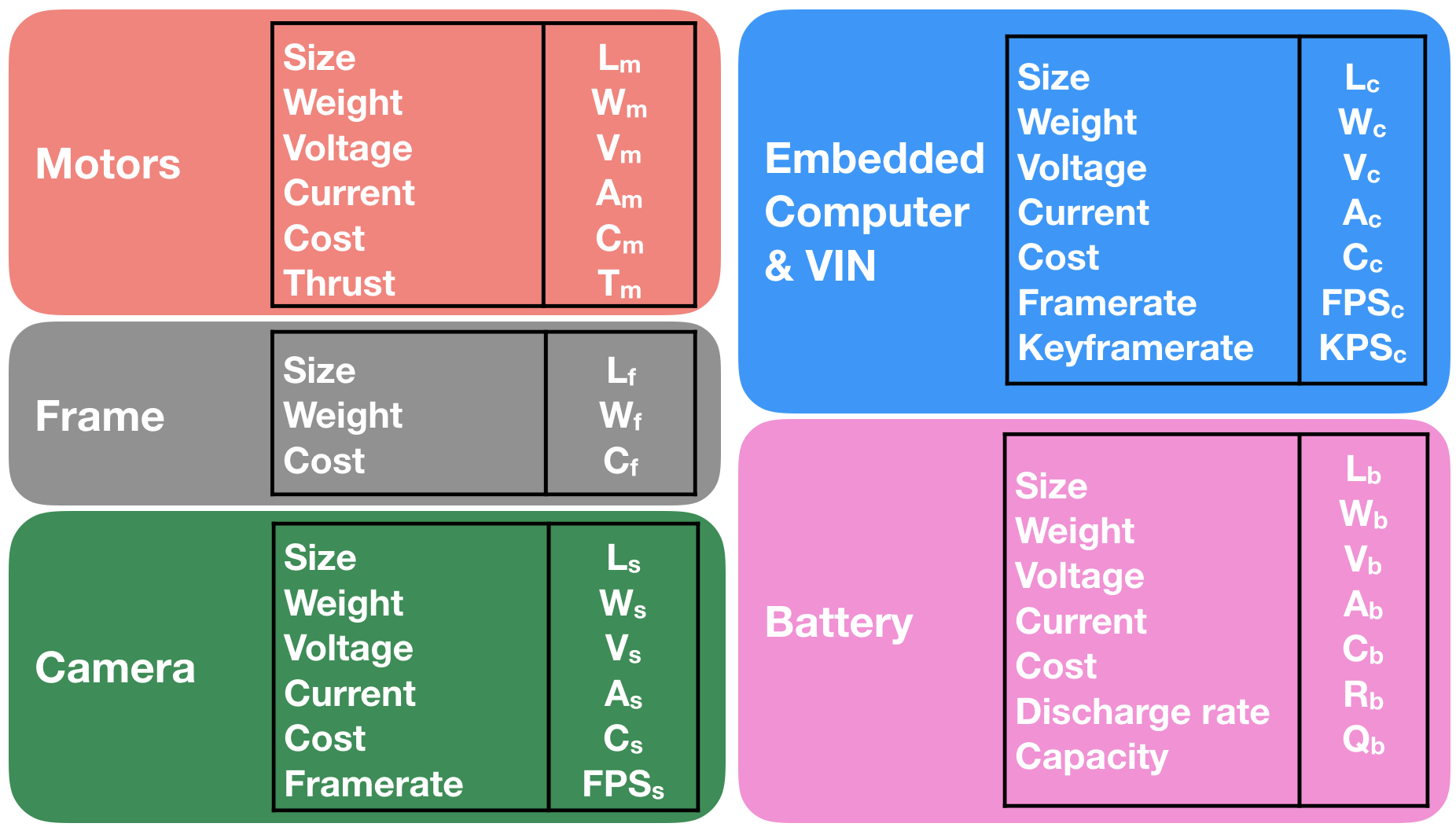
Figure 2: Drone co-design overview: modules and features.

An overview of the modules we design and their corresponding features is given in Fig. 2. For the sake of simplicity, in this toy example we preferred not to design other components. For instance, we disregarded other algorithms running on the board, e.g., for control, which are typically less computationally demanding. We also neglected the presence/design of voltage adapters and connectors, while we assumed that each choice of motors comes with a suitable choice of ESC (Electronic Speed Control boards) and propellers.

System-level performance. The second step of the design process is to quantitatively define the system-level performance metrics (what is the “best drone”?). Since we consider an autonomous drone racing application, the best drone is one that can complete a given track as quickly as possible, hence a system that can navigate at high speed. Therefore, in this example, the system performance metric is the top speed of the drone. We mainly consider forward speed, but the presentation can be extended to maximize agility and accelerations.

In order to derive an expression for the top (forward) speed, we observe Fig. 1(b) and note that at its top speed, the forward acceleration is zero, hence the horizontal component $T_{h}$ of the thrust $T$ must compensate the drag force (i) $T_{h}=D$, and the vertical component $T_{v}$ of the thrust must compensate the force of gravity (ii) $T_{v}=F_{g}=Mg$, where $M$ is the overall mass of the drone and $g$ is the acceleration due to gravity. Let us focus on (i), and note that (iii) $T^{2}=T_{h}^{2}+T_{v}^{2}$ and that the drag can be modeled as (iv) $D=\frac{1}{2}\rho c_{d}Av^{2}$, where $\rho$ is the air density, $c_{d}$ is the drag coefficient (we take $\rho=1.2\text{kg}/\text{m}^{3}$ and $c_{d}=1.3$), $A$ is the cross-sectional area, and $v$ is the forward speed of the drone. Substituting (ii), (iii), and (iv) back into (i), we obtain:

$$\sqrt{T^{2}-(Mg)^{2}}=\frac{1}{2}\,\rho\,c_{d}\,A\,v_{\max}^{2}$$ (34)

Now we note that the cross-sectional area can be approximated as $A=\sin(\beta)\ell^{2}=\frac{Mg}{T}L_{\text{f}}^{2}$, where $\beta$ is the pitch angle (basic trigonometry shows $\sin(\beta)=\frac{Mg}{T}$), and $L_{\text{f}}$ is the length of the frame (approximated as a square). Substituting this expression for $A$ in (34) and rearranging the terms we obtain:

$$v_{\max}=\left(\frac{4T^{2}}{\rho^{2}c_{d}^{2}L_{\text{f}}^{4}}\left(\frac{T^{2}}{(Mg)^{2}}-1\right)\right)^{\frac{1}{4}}$$ (35)

Finally, assuming that we design a quadrotor, the cumulative thrust is the sum of the thrusts $T_{\text{m}}$ provided by each of the four motors, while the mass is the sum of the weight $W_{i}$ of all the modules $i\in{\cal M}$:

$$v_{\max}=\left(\frac{4(4T_{\text{m}})^{2}}{\rho^{2}c_{d}^{2}L_{\text{f}}^{4}}\left(\frac{(4T_{\text{m}})^{2}}{(g\sum_{i\in{\cal M}}\omega_{i}W_{i})^{2}}-1\right)\right)^{\frac{1}{4}}$$ (SP)

where $\omega_{i}=4$ if $i=\text{m}$ (we have 4 motors on a quadrotor, each one weighting $W_{\text{m}}$), or $\omega_{i}=1$ otherwise.

In order to make explicit that the values of $T_{\text{m}},W_{i},L_{\text{f}}$ depend on our design, we observe that $T_{\text{m}}=[{\bm{F}}_{\text{m}}]_{T}{\bm{x}}_{\text{m}}$, $W_{i}=[{\bm{F}}_{i}]_{W}{\bm{x}}_{i}$ $L_{\text{f}}=[{\bm{F}}_{\text{f}}]_{L}{\bm{x}}_{\text{f}}$, which makes (SP) a function of our design vector. Eq. (SP) represents the system performance metric our design has to maximize. It is apparent from (SP) that the design encourages drones which are small and lightweight ($L_{\text{f}}$ and $W_{i}$ appear at the denominator) and with large thrust ($T_{\text{m}}$ appears at the numerator).

System-level constraints. System constraints provide further specifications (in the form of hard constraints) on the task the drone is designed for. For our drone example, we consider two main constraints: monetary budget and flight time.

1. Budget: Given a monetary budget $\bar{b}$, the budget constraint enforces that the sum of the costs $C_{i}$ of each module $i$ is within the budget:

   $$\textstyle\sum_{i\in{\cal M}}\omega_{i}C_{i}\leq\bar{b}$$ (SC1)

   where again $\omega_{i}=4$ if $i=\text{m}$ or $\omega_{i}=1$ otherwise.

2. Flight time: Given a minimum flight time $\bar{T}$ (this would be between 5-10 minutes in a real application), and calling $Q_{\text{b}}$ the battery capacity, and $A_{i}$ the average Ampere drawn by the $i$-th component (all assumed to operate at the same voltage), then the time it takes to drain the battery must be $\geq\bar{T}$:

   $$\frac{\alpha Q_{\text{b}}}{\sum_{i\in{\cal M}}\omega_{i}A_{i}}\geq\bar{T}$$ (SC2)

   where $\omega_{i}=4$ if $i=\text{m}$ (again, we have 4 motors on a quadrotor), or $\omega_{i}=1$ otherwise; the constant $\alpha\in(0,1]$ (typically chosen to be around $0.8$) models the fact that we might not want to fully discharge our battery (e.g., LiPo batteries may be damaged when discharged below a recommended threshold).

We remark that while flight time and budget constraints already make for an interesting problem, one can come up with many more system constraints, e.g., size and weight limits to participate into a specific drone racing competition, or motor power constraints for safety or regulatory constraints.

Implicit (module-level) constraints. The implicit constraints make sure that each module can operate correctly and it is compatible with the other modules in the system. We identified five implicit constraints:

1. Minimum thrust: the cumulative thrust provided by the four motors has to be sufficient for flight. Calling $T_{\text{m}}$ the thrust provided by each motor, and $W_{i}$ the weight of the $i$-th module, the minimum thrust constraint can be written as:

   $$4T_{\text{m}}\geq\bar{r}\;g\sum_{i\in{\cal M}}\omega_{i}W_{i}$$ (IC1)

   where $\bar{r}$ is a given minimum thrust-weight ratio ($\bar{r}=2$ in this example), to ensure that the thrust is sufficient to maneuver with agility, besides allowing the drone to hover.

2. Power: the battery should provide enough power to support the four motors, the camera, and the computer:

   $$A_{\text{b}}V_{\text{b}}\geq 4A_{\text{m}}V_{\text{m}}+A_{\text{s}}V_{\text{s}}+A_{\text{c}}V_{\text{c}}$$ (IC2)

   where $A_{i},V_{i}$ are the current and voltage for the $i$-th module.

3. Size: all components should fit on the frame. Assuming we can stack components on top of each other, the size constraint enforces that the size of each component should be smaller than the size of the frame:

   $$L_{\text{f}}\geq L_{i}\quad\text{with }i\in\{\text{m},\text{s},\text{c},\text{b}\}$$ (IC3)

4. Minimum camera frame-rate: the framerate of the camera should be fast enough to allow tracking visual features, during fast motion. This is necessary for the visual-inertial navigation (VIN) algorithms to properly estimate position and attitude of the drone. Assuming that our VIN front-end can track a feature moving by at most $\delta_{u}$ pixels between frames, and corresponding to the projection of a 3D point at distance $d$ from the camera (we assume $\delta_{u}=30$ pixels, $d=5$ meters), the frame-rate $\text{FPS}_{s}$ of the camera is bounded by [1]:

   $$\text{FPS}_{s}\geq\frac{fv_{\max}}{\delta_{u}d}$$ (IC4)

   where $f$ is the focal length of the camera, and $v_{\max}$ is the maximum speed of the drone, given in (SP).

5. Minimum VIN frame-rate: the VIN algorithm operating on the embedded computer on the drone should be able to process each frame, hence the VIN frame-rate (recall that we select from a catalog of VIN+computer combinations) must be larger than the camera frame-rate:

   $$\text{FPS}_{c}\geq\text{FPS}_{s}$$ (IC5)

Implementation and results. The “optimal” drone design solves the following optimization problem:

$$\begin{array}[]{lll}\;\;\;\max_{{\bm{x}}\in{\cal X}}&\text{(SP)}\\ \text{ subject to }&\text{(SC1)},\text{(SC2)}\\ &\text{(IC1)},\text{(IC2)},\text{(IC3)},\text{(IC4)},\text{(IC5)}\end{array}$$ (36)

Most of the constraints are already in a form that is amenable for our approach (Sec. III). Only the objective (SP) and the constraints (SC2) and (IC4) have a more involved expression, which we further develop in the appendix, where we show how to approximate those expressions in a form that fit a linear co-design solver.

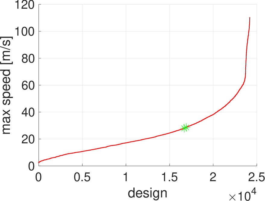
(a)

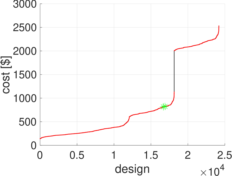
(b)

Figure 3: (a) Estimated maximum speed and (b) cost for any potential configuration of modules in our catalog. Infeasible designs are marked in red, while feasible designs are marked with a green star.

The optimal design we found in our implementation suggests that an optimal configuration of modules would include a Stormer 220 FPV Racing Quadcopter Frame Kit, EMAX1045 motors, an NVIDIA TX2 computer, a 60 frame-per-second camera, and a Tattu 5100mAh 3S 10C Battery Pack. The cost of such a drone would be $\$700.84$, and the drone would have a flight time of $10.42$ minutes and a top speed of $35.52$ meters per second, which is compatible with the performance one expects from a racing drone [21]. CPLEX was able to find an optimal design in $0.3$ seconds. Since the design space is relatively small we can compute the estimated maximum speed and the cost of every potential combination of the modules in our catalog. These results are shown in Fig. 3, where we also report whether the configuration is feasible (it satisfied all system and implicit constraints) or not. The figure shows that there are indeed only four feasible designs in our catalog all attaining fairly similar performance and cost.

IV-B Codesign of Heterogeneous Multi-Robot Teams

This section applies the proposed framework to the co-design of a heterogeneous multi-robot team. In particular, we consider a collective transport scenario, in which the robots must collectively carry a heavy object while avoiding obstacles. The robots must be configured to allow for efficient carrying and for wide sensor coverage, while battery power and frame size constrain the capabilities that any single robot possesses. The end result of our design is a heterogeneous team, composed of robots that specialize in carrying and robots that specialize in sensing. As a simplifying assumption, we focus on objects and robots with circular shapes (see Fig. 4).

Modules. We consider four types of modules: frames (f), sensors (s), motors (m), and batteries (b). Frames’ features include size and weight; sensors’ features include coverage (as a percentage of the surrounding area), size, weight, and power consumption; motors’ features include weight, size, power consumption and force exerted; and batteries’ features include size, weight, and power generated.

Since we have to design multiple robots, we use the notation ${\bm{x}}^{k}_{i}$ to denote the design vector associated to the $i$-th module of robot $k$. As before, we use $[{\bm{x}}^{k}_{i}]_{j}$ to denote the $j$-th entry of ${\bm{x}}^{k}_{i}$. $[{\bm{x}}^{k}_{i}]_{j}=1$ if we chose the $j$-th element in the catalog ${\cal C}_{i}$ of module $i$ on robot $k$, or zero otherwise. We let $k\in\{1,\ldots,K\}$ where we calculate the upper bound $K$ by considering the maximum number of robots that can encircle the object when the smallest frame is used. If the radius of the object is $R^{\text{object}}$ and the radius of the smallest frame is $R^{\text{min frame}}$, then

$$K=\left\lfloor\frac{\pi(R^{\text{object}}+R^{\text{min frame}})}{R^{\text{min frame}}}\right\rfloor.$$ (37)

System-level performance. In a multi-robot system, performance is inherently non-monotonic. In Hamann’s analysis [15], performance is expressed as the ratio of two components: cooperation $C({\bm{x}})$ and interference $I({\bm{x}})$. Cooperation refers to those phenomena that contribute to the task at hand; interference corresponds to the phenomena that diminish the system performance. A simple approach to capture both aspects is to cast the co-design problem as an interference minimization problem, while using cooperation measures as system constraints. In [15], $I({\bm{x}})$ is expressed as an exponential that decays with the size of the team $R$, from which it follows

$$\min_{{\bm{x}}\in{\cal X}}I({\bm{x}})\equiv\min_{{\bm{x}}\in{\cal X}}{\mathrm{e}}^{R({\bm{x}})}\equiv\min_{{\bm{x}}\in{\cal X}}R({\bm{x}})\equiv\max_{{\bm{x}}\in{\cal X}}-R({\bm{x}})$$ (38)

where the symbol “$\equiv$” denotes that these changes of objective do not alter the solution of the optimization problem. In (38) we also observed that the team size is a function of our design ($R=R({\bm{x}})$), i.e., the design algorithm can decide to use less robots than the upper bound (37). Eq. (38) shows that our design will attempt to use the least number of robots, in order to minimize interference. To capture $R({\bm{x}})$, we augment ${\bm{x}}$ with a binary element (later called the “slot”) that indicates whether the features of a robot $k$ are being used or not (in other words: if the robot is part of the team of not). We can thus define $R({\bm{x}})=\sum_{k=1}^{K}{\bm{x}}^{k}_{\text{slot}}$ and write

$$\text{SP}({\bm{x}})=-\textstyle\sum_{k=1}^{K}{\bm{x}}^{k}_{\text{slot}}.$$ (SP)

System-level constraints. We consider two families of system constraints concerning motors and sensing.

1. Push for object transportation: the team as a whole must be able to carry the object; this is essentially the cooperation measure mentioned above. For this, we need that the push $P_{j}$ exerted by the choice of motor $j$ exceeds the sum of the weights $W_{i,j}$ of each choice modules ($i\in{\cal M}$ and $j\in{\cal C}_{i}$) plus the weight $W$ of the object to transport:

   $$\sum_{k\in\{1,\ldots,K\},j\in{\cal C}_{\text{m}}}P_{j}[{\bm{x}}^{k}_{\text{m}}]_{j}\geq\sum_{k\in\{1,\ldots,K\},i\in\mathcal{M},j\in{\cal C}_{i}}W_{i,j}[{\bm{x}}^{k}_{i}]_{j}+W$$ (SC1)

   In addition, each robot’s motor push must exceed the weight of the robot itself:

   $$\sum_{j\in{\cal C}_{\text{m}}}P_{j}[{\bm{x}}^{k}_{\text{m}}]_{j}\geq\!\!\!\sum_{i\in\mathcal{M},j\in{\cal C}_{i}}\!\!\!W_{i,j}[{\bm{x}}^{k}_{i}]_{j}\quad\forall k\in\{1,\ldots,K\}$$ (SC2)

2. Sensor coverage: the robot sensors must ensure that at least 50% of the area around the object is covered at any time:

   $$\sum_{j\in{\cal C}_{\text{s}}}S_{j}[{\bm{x}}^{k}_{\text{s}}]_{j}\geq 50\%$$ (SC3)

   where $S_{j}$ is the coverage provided by the $j$-th sensor choice.

TABLE I: Implicit constraints for the multi-robot co-design example.

Meaning	Formalization	Tag
If a slot is activated, the robot has one frame	$\forall k\quad{\bm{x}}^{k}_{\text{slot}}=\sum_{j\in{\cal C}_{\text{f}}}[{\bm{x}}^{k}_{\text{f}}]_{j}$	(IC1)
If a slot is activated, the robot has one motor	$\forall k\quad{\bm{x}}^{k}_{\text{slot}}=\sum_{j\in{\cal C}_{\text{m}}}[{\bm{x}}^{k}_{\text{m}}]_{j}$	(IC2)
If a slot is activated, the robot has one battery	$\forall k\quad{\bm{x}}^{k}_{\text{slot}}=\sum_{j\in{\cal C}_{\text{b}}}[{\bm{x}}^{k}_{\text{b}}]_{j}$	(IC3)
If a slot is activated, the robot has at most one sensor	$\forall k\quad{\bm{x}}^{k}_{\text{slot}}\geq\sum_{j\in{\cal C}_{\text{s}}}[{\bm{x}}^{k}_{\text{s}}]_{j}$	(IC4)
The power consumption of a robot is lower than the power given by the battery	$\forall k\quad\sum_{j\in{\cal C}_{\text{b}}}P_{\text{b},j}[{\bm{x}}^{k}_{\text{b}}]_{j}\geq\sum_{i\in\{\text{m},\text{s}\},j\in{\cal C}_{i}}P_{i,j}[{\bm{x}}^{k}_{i}]_{j}$	(IC5)
The total size of the components of a robot is lower than the size of the chassis	$\forall k\quad\sum_{j\in{\cal C}_{\text{f}}}A_{\text{f},j}[{\bm{x}}^{k}_{\text{f}}]_{j}\geq\sum_{i\in\{\text{m},\text{s},\text{b}\},j\in{\cal C}_{i}}A_{i,j}[{\bm{x}}^{k}_{i}]_{j}$	(IC6)

Implicit (module-level) constraints. Table I summarizes the implicit constraints in our example. The symbol $P_{i,j}$ denotes the power offered by battery $j$ or used by the $j$-th choice of module $i$. $A_{i,j}$ denotes the area offered by a frame $j$ or the area used by the $j$-th choice of module $i$.

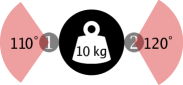
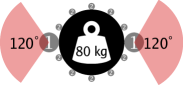
Figure 4: Collective transport example (top view), where multiple robots (gray circles) carry a large object (black circle). The figure shows two solutions found by CPLEX when the object weighs $10\,\mathrm{kg}$ (left) and $80\,\mathrm{kg}$ (right).

Implementation and results. To form the catalog of possible modules, we considered 10 alternatives for each type of module and 2 alternatives for the size of the robot frame, for a total of $2,000$ combinations. Using the size and weight of the object to transport, we explored the space of optimal solutions, which involved teams of up to $K=65$ robots. Fig. 4 reports the solutions we found by solving two instances of the problem, where the object to carry weighted $10\,\mathrm{kg}$ and $80\,\mathrm{kg}$, respectively. In the left diagram, CPLEX concluded that two large robots are sufficient to carry a $10\,\mathrm{kg}$ object. The robots are equipped with identical motors and batteries, and differ only in their sensor coverage. In the right diagram, CPLEX generated a solution including two types of robots: the larger type offers a lower pushing margin, but is capable of wide sensing; the smaller type is lighter and offers a higher pushing margin, but it performs no sensing. The presence of robots that carry no sensors allows them to collectively shoulder the bulk of the pushing. The interested reader can find the complete CPLEX implementation at https://bitbucket.org/lucacarlone/codesigncode/.

V Conclusion

We presented an approach for computational robot co-design that formulates the joint selection of the modules composing a robotic system in terms of mathematical programming. While our approach is rooted in the general context of binary optimization, we discussed a number of properties—specific to our co-design problem—that allow rephrasing several co-design problems including non-linear functions of the features of each module in terms of binary linear programming (BLP). Modern BLP algorithms and implementations can solve problems with few thousands of variables in seconds, which in turn allows attacking interesting co-design problems. We demonstrated the proposed co-design approach in two applications: the design of an autonomous drone and the design of a multi-robot team for collective transportation. Future work includes extending the set of functions for which we can solve the co-design problem in practice, and adding continuous variables (e.g., wing length, 3D-printed frame size) as part of the co-design problem.

-A Drone Co-design

This section discusses how to approximate the objective (SP) and the constraints (SC2) and (IC4) using binary linear functions. The following paragraphs deal with each case.

A linear lower bound for the objective (SP). The design has to maximize the maximum forward speed, which, from (SP), has the following expression:

$$v_{\max}=\left(\frac{4(4T_{\text{m}})^{2}}{\rho^{2}c_{d}^{2}L_{\text{f}}^{4}}\left(\frac{(4T_{\text{m}})^{2}}{(g\sum_{i\in{\cal M}}\omega_{i}W_{i})^{2}}-1\right)\right)^{\frac{1}{4}}$$ (39)

This expression does not fall in cases (a), (b), (c) in Section III; moreover, it involves all modules, hence taking the approach (d) of Section III would be impractical (it would simply lead to enumerating every possible design choice, implying a combinatorial explosion of the state space).

The approach we take in this section is to approximate Problem (36) by replacing its objective with a linear lower bound. We remark that, as shown in Section III, while the design is required to be linear in ${\bm{x}}$, it can be heavily nonlinear in the features ${\bm{F}}_{i}$. In the following we show how to obtain a linear lower bound for (39). For this purpose, we observe that from (IC1), the thrust-weight ratio must be larger than $\bar{r}$, hence $(4T_{\text{m}})/(g\sum_{i\in{\cal M}}\omega_{i}W_{i})\geq\bar{r}$. Therefore, it holds:

$$v_{\max}=\left(\frac{4(4T_{\text{m}})^{2}}{\rho^{2}c_{d}^{2}L_{\text{f}}^{4}}\left(\frac{(4T_{\text{m}})^{2}}{(g\sum_{i\in{\cal M}}\omega_{i}W_{i})^{2}}-1\right)\right)^{\frac{1}{4}}$$

$$\geq\left(\frac{4(4T_{\text{m}})^{2}}{\rho^{2}c_{d}^{2}L_{\text{f}}^{4}}\left(\bar{r}^{2}-1\right)\right)^{\frac{1}{4}}=\kappa\frac{T_{\text{m}}^{\frac{1}{2}}}{L_{\text{f}}}=\kappa\frac{([{\bm{F}}_{\text{m}}]_{T}\,{\bm{x}}_{\text{m}})^{\frac{1}{2}}}{[{\bm{F}}_{\text{f}}]_{L}{\bm{x}}_{\text{f}}}$$ (40)

where $\kappa$ is a constant, irrelevant for the maximization. The function (40) now falls in the case (c) discussed in Section III and can be made linear in ${\bm{x}}$ by taking the logarithm.

A conservative linear approximation for (IC4). Similarly to the case discussed above, we approximate the “problematic” constraints via surrogates that are linear in ${\bm{x}}$.

The approach we take is to substitute a constraint in the form $f({\bm{x}})\leq 0$ with a linear constraint $\hat{f}({\bm{x}})\leq 0$, where $f({\bm{x}})\leq\hat{f}({\bm{x}})$ for any ${\bm{x}}\in{\cal X}$. This guarantees that for any ${\bm{x}}$ that makes $\hat{f}({\bm{x}})\leq 0$, then also $f({\bm{x}})\leq 0$, i.e., we still guarantee to compute feasible (but potentially more conservative) designs.

Therefore, in the following we show how to obtain a linear upper bound for (IC4). Let us start by writing (IC4) more explicitly, by substituting $v_{\max}$ from (19):

$$\text{FPS}_{\text{s}}\geq\frac{f}{\delta_{u}d}\left(\frac{4(4T_{\text{m}})^{2}}{\rho^{2}c_{d}^{2}L_{\text{f}}^{4}}\left(\frac{(4T_{\text{m}})^{2}}{(g\sum_{i\in{\cal M}}\omega_{i}W_{i})^{2}}-1\right)\right)^{\frac{1}{4}}$$ (41)

or equivalently (taking the $4$-th power of each member):

$$\text{FPS}_{\text{s}}^{4}\geq\frac{4f^{4}}{\delta_{u}^{4}d^{4}\rho^{2}c_{d}^{2}}\frac{(4T_{\text{m}})^{2}}{L_{\text{f}}^{4}}\left(\frac{(4T_{\text{m}})^{2}}{(g\sum_{i\in{\cal M}}\omega_{i}W_{i})^{2}}-1\right)$$ (42)

Taking the logarithm of both sides we obtain:

$$4\log(\text{FPS}_{\text{s}})\geq\beta+2\log(4T_{\text{m}})-4\log(L_{\text{f}})+$$

$$+\log\left(\frac{(4T_{\text{m}})^{2}}{(g\sum_{i\in{\cal M}}\omega_{i}W_{i})^{2}}-1\right)$$ (43)

where we defined the constant $\beta\doteq\log(\frac{4f^{4}}{\delta_{u}^{4}d^{4}\rho^{2}c_{d}^{2}})$.

Rearranging the terms:

$$2\log(4T_{\text{m}})-4\log(L_{\text{f}})+$$

$$+\log\left(\frac{(4T_{\text{m}})^{2}}{(g\sum_{i\in{\cal M}}\omega_{i}W_{i})^{2}}-1\right)-4\log(\text{FPS}_{\text{s}})+\beta\leq 0$$ (44)

We note that so far we did not take any approximation since each operation we applied ($4$-th power, logarithm, reordering) preserves the original inequality. Moreover, (44) is in the form $f({\bm{x}})\leq 0$. In the rest of this paragraph, we show how to compute a linearized upper bound for $f({\bm{x}})$. For this purpose we note that the following chain of inequalities holds:

$$2\log(4T_{\text{m}})-4\log(L_{\text{f}})+$$

$$+\log\left(\frac{(4T_{\text{m}})^{2}}{(g\sum_{i\in{\cal M}}\omega_{i}W_{i})^{2}}-1\right)-4\log(\text{FPS}_{\text{s}})+\beta\!\! \!\!\!\!\overset{(i)}{\leq}\!\!\!\!$$

$$2\log(4T_{\text{m}})-4\log(L_{\text{f}})+$$

$$+\log\left(\frac{(4T_{\text{m}})^{2}}{(g\sum_{i\in{\cal M}}\omega_{i}W_{i})^{2}}\right)-4\log(\text{FPS}_{\text{s}})+\beta\!\! \!\!\!\!\overset{(ii)}{=}\!\!\!\!$$

$$4\log(4T_{\text{m}})-4\log(L_{\text{f}})+$$

$$-2\log\left(\sum_{i\in{\cal M}}g\,\omega_{i}\,W_{i}\right)-4\log(\text{FPS}_{\text{s}})+\beta\!\! \!\!\!\!\overset{(iii)}{\leq}\!\!\!\!$$

$$4\log(4T_{\text{m}})-4\log(L_{\text{f}})+$$

$$-2\sum_{i\in{\cal M}}\frac{1}{|{\cal M}|}\log\left(g\,\omega_{i}\,W_{i}\right)\!-\!2\log(|{\cal M}|)\!-\!4\log(\text{FPS}_{\text{s}})+\beta$$ (45)

where in (i) we dropped the $-1$ and used the fact that the logarithm is a non-decreasing function, in (ii) we simply developed the logarithm of the ratio, and in (iii) we used the Jensen’s inequality:

$$\log\left(\frac{\sum_{i=1}^{n}y_{i}}{n}\right)\geq\frac{\sum_{i=1}^{n}\log(y_{i})}{n}\iff$$ (46)

$$\log\left(\sum_{i=1}^{n}y_{i}\right)\geq\sum_{i=1}^{n}\frac{1}{n}\log(y_{i})+\log(n)$$ (47)

which holds for any integer $n$ and positive scalar $y_{i}$.

Making the dependence of $T_{\text{m}}$, $L_{\text{f}}$, $W_{i}$, and $\text{FPS}_{\text{s}}$ on the design vector ${\bm{x}}$ explicit in (45), we obtain:

$$\hat{f}({\bm{x}})\doteq 4\log(4[{\bm{F}}_{\text{m}}]_{T}{\bm{x}}_{\text{m}})-4\log([{\bm{F}}_{\text{f}}]_{L}{\bm{x}}_{\text{f}})+$$

$$-2\sum_{i\in{\cal M}}\frac{1}{|{\cal M}|}\log\left(g\,\omega_{i}\,[{\bm{F}}_{i}]_{W}{\bm{x}}_{i}\right)+$$

$$-2\log(|{\cal M}|)-4\log([{\bm{F}}_{\text{s}}]_{\text{FPS}}{\bm{x}}_{\text{s}})+\beta$$ (48)

which now falls in the case (b) discussed in Section III and can be easily made linear with respect to ${\bm{x}}$.

A conservative linear approximation for (SC2). Similarly to the previous section, here we approximate the “problematic” constraint (SC2) via surrogates that are linear in ${\bm{x}}$. In particular, as before, we substitute a constraint in the form $f({\bm{x}})\leq 0$ with a linear constraint $\hat{f}({\bm{x}})\leq 0$, where $f({\bm{x}})\leq\hat{f}({\bm{x}})$ for any ${\bm{x}}\in{\cal X}$. This guarantees that for any ${\bm{x}}$ that makes $\hat{f}({\bm{x}})\leq 0$, then also $f({\bm{x}})\leq 0$, i.e., we still guarantee to compute feasible (but potentially more conservative) designs.

Let us start by reporting the original expression we want to approximate (SC2):

$$\frac{\alpha Q_{\text{b}}}{\sum_{i\in{\cal M}}\omega_{i}A_{i}}\geq\bar{T}$$ (49)

which, again, does not fall in cases (a), (b), (c) in Section III, and involves all modules, hence making the approach described in case (d) of Section III impractical.

In order to obtain a conservative approximation of the constraint (49), we first take the logarithm of both members:

$$\log(\alpha Q_{\text{b}})-\log\left(\sum_{i\in{\cal M}}\omega_{i}A_{i}\right)\geq\log(\bar{T})$$ (50)

which does not alter the inequality since all involved quantities are positive. Rearranging the terms:

$$\log\left(\sum_{i\in{\cal M}}\omega_{i}A_{i}\right)-\log(\alpha Q_{\text{b}})+\log(\bar{T})\leq 0$$ (51)

We can find an upper bound for the left-hand-side of (51) as follows:

$$\log\left(\sum_{i\in{\cal M}}\omega_{i}A_{i}\right)-\log(\alpha Q_{\text{b}})+\log(\bar{T})\leq$$

$$\log(6A_{\text{m}})-\log(\alpha Q_{\text{b}})+\log(\bar{T})$$ (52)

where we used $\sum_{i\in{\cal M}}\omega_{i}A_{i}=A_{\text{s}}+A_{\text{c}}+4A_{\text{m}}\leq 6A_{\text{m}}$ (note: frame and batteries are assumed to draw zero current) which follows from the fact the motors are the modules that draw more current. Therefore we can substitute the original constraint (49) with a conservative linear approximation:

$$\hat{f}({\bm{x}})\doteq\log(6[{\bm{F}}_{\text{m}}]_{A}{\bm{x}}_{\text{m}})-\log(\alpha[{\bm{F}}_{\text{b}}]_{Q}{\bm{x}}_{\text{b}})+\log(\bar{T})\leq 0$$ (53)

which now falls in the case (b) discussed in Section III and can be easily made linear with respect to ${\bm{x}}$.

References

- [1] Z. Zhang, A. Suleiman, L. Carlone, V. Sze, and S. Karaman, “Visual-inertial odometry on chip: An algorithm-and-hardware co-design approach,” in Robotics: Science and Systems (RSS), 2017.
- [2] NVIDIA, “Nvidia jetson tx2 module specifications.” [Online]. Available: https://developer.nvidia.com/embedded/buy/jetson-tx2
- [3] D. Lipinski and K. Mohseni, “Feasible area coverage of a hurricane using micro-aerial vehicles,” in AIAA Scitech, 2014, pp. 824–829.
- [4] H. Lipson and J. B. Pollack, “Automatic design and manufacture of robotic lifeforms,” Nature, vol. 406, no. 6799, pp. 974–978, Aug. 2000.
- [5] H. Lipson, V. Sunspiral, J. Bongard, and N. Cheney, “On the difficulty of co-optimizing morphology and control in evolved virtual creatures,” in Proceedings of the European Conference on Artificial Life 13. MIT Press, 2016, pp. 226–233.
- [6] N. Cheney, J. Bongard, V. SunSpiral, and H. Lipson, “Scalable co-optimization of morphology and control in embodied machines,” Journal of The Royal Society Interface, vol. 15, no. 143, p. 20170937, June 2018.
- [7] P. H. Chou, R. B. Ortega, and G. Borriello, “The Chinook Hardware/Software Co-synthesis System,” in Proceedings of the 8th International Symposium on System Synthesis, ser. ISSS ’95. New York, NY, USA: ACM, 1995, pp. 22–27.
- [8] B. C. Schafer and K. Wakabayashi, “Divide and Conquer High-level Synthesis Design Space Exploration,” ACM Trans. Des. Autom. Electron. Syst., vol. 17, no. 3, pp. 29:1–29:19, July 2012.
- [9] “Architecture Analysis and Design Language.” [Online]. Available: http://www.aadl.info/aadl/currentsite/
- [10] A. Mehta, J. DelPreto, and D. Rus, “Integrated Codesign of Printable Robots,” Journal of Mechanisms and Robotics, vol. 7, no. 2, pp. 021 015–021 015–10, May 2015.
- [11] O. Hussien, A. Ames, and P. Tabuada, “Abstracting Partially Feedback Linearizable Systems Compositionally,” IEEE Control Systems Letters, vol. 1, no. 2, pp. 227–232, Oct. 2017.
- [12] E. S. Kim, M. Arcak, and M. Zamani, “Constructing Control System Abstractions from Modular Components,” in Proceedings of the 21st International Conference on Hybrid Systems: Computation and Control (Part of CPS Week), ser. HSCC ’18. New York, NY, USA: ACM, 2018, pp. 137–146.
- [13] A. Censi, “A Mathematical Theory of Co-Design,” arXiv:1512.08055 [cs, math], Dec. 2015, arXiv: 1512.08055.
- [14] ——, “A Class of Co-Design Problems With Cyclic Constraints and Their Solution,” IEEE Robotics and Automation Letters, vol. 2, no. 1, pp. 96–103, Jan. 2017.
- [15] H. Hamann, “Towards Swarm Calculus: Universal Properties of Swarm Performance and Collective Decisions,” in Swarm Intelligence, D. e. a. Hutchison, Ed. Berlin, Heidelberg: Springer Berlin Heidelberg, 2012, vol. 7461, pp. 168–179.
- [16] A. Kushleyev, D. Mellinger, C. Powers, and V. Kumar, “Towards a swarm of agile micro quadrotors,” Autonomous Robots, vol. 35, no. 4, pp. 287–300, 2013.
- [17] V. Trianni, Evolutionary Swarm Robotics - Evolving Self-Organising Behaviours in Groups of Autonomous Robots, ser. Studies in Computational Intelligence. Springer, 2008, vol. 108.
- [18] G. Francesca, M. Brambilla, A. Brutschy, L. Garattoni, R. Miletitch, G. Podevijn, A. Reina, T. Soleymani, M. Salvaro, C. Pinciroli, F. Mascia, V. Trianni, and M. Birattari, “AutoMoDe-Chocolate: automatic design of control software for robot swarms,” Swarm Intelligence, vol. 9, no. 2, pp. 125–152, Sept. 2015.
- [19] A. Schrijver, Theory of Linear and Integer Programming. New York, NY, USA: John Wiley & Sons, Inc., 1986.
- [20] IBM, “CPLEX: IBM ILOG CPLEX Optimiz Studio.” [Online]. Available: https://www.ibm.com/products/ilog-cplex-optimization-studio
- [21] FPV Drone Reviews, “Fastest FPV drones, https://fpvdronereviews.com/guides/fastest-racing-drones/,” 2017.