Taylor expansion based fast Multipole Methods for 3-D Helmholtz equations in Layered Media

Abstract

In this paper, we develop fast multipole methods for 3D Helmholtz kernel in layered media. Two algorithms based on different forms of Taylor expansion of layered media Green’s function are developed. A key component of the first algorithm is an efficient algorithm based on discrete complex image approximation and recurrence formula for the calculation of the layered media Green’s function and its derivatives, which are given in terms of Sommerfeld integrals. The second algorithm uses symmetric derivatives in the Taylor expansion to reduce the size of precomputed tables for the derivatives of layered media Green’s function. Numerical tests in layered media have validated the accuracy and $O(N)$ complexity of the proposed algorithms.

1 Introduction

Wave scattering of objects embedded in layered media can be computed by integral equation (IE) methods using domain Green’s functions which satisfy the transmission conditions at material layer interfaces and the Sommerfeld radiation condition at infinity (cf. [1, 2, 3, 4]). As a result, IE methods based on domain Green’s functions only require solution unknowns to be given on the scatterer’s surface for a surface IE formulation or over the scatterer body for a volume IE. This is different from formulations based on free space Green’s functions, which will need additional unknowns on the infinite material layer interfaces (cf. [6, 7, 8]). For the solution of the resulting linear system from the discretized IEs, iterative solvers such as GMRES are usually used, which require the product of a full matrix, from the discretization of the integral operator, and a solution vector. A direct product will generate an $O(N^{2})$ cost where $N$ is the size of the matrix. Therefore, the main computational issue for IE methods is to develop fast solvers to speed up such a matrix-vector product. The popular fast method is the fast multipole method (FMM) developed by Greengard and Rokhlin using multipole expansions for the free space Green’s functions [9, 10]. However, extending FMMs to layered media has been a long outstanding challenge for IE methods.

Numerical algorithms for layered-media problems have traditionally been carried out in the Fourier spectral domain due to the availability of the closed-form Green’s functions (CFGF’s) for layered media in the spectral domain. Since a series of techniques have been developed to obtain approximated CFGF’s for layered media in the spatial domain (cf. [11, 12, 13]), extensions of FMMs to layered media problems were proposed by applying spherical harmonic expansions to the approximated CFGF’s (see [14, 15, 16] for Laplace, Helmholtz and Maxwell’s equations, respectively). For the Laplace equation, only real images were used in the approximating the CFGF’s and traditional FMMs can be then applied to the approximated CFGF’s, directly. However, for Helmholtz and Maxwell’s equations in layered media, complex images are required to obtain approximated CFGF’s. Thus, addition theorems used for the free space FMMs need  to be modified for wave functions with complex arguments, so far no rigorous mathematical formulations and numerical implementation have been obtained. Other efforts to speed up the computation of integral operator for layered media Green’s functions include the inhomogeneous plane wave method [38], windowed Green’s function method for layered-media [39], and cylindrical wave decomposition of the Green’s function in 3-D and 2-D FMM [5].

In this paper, we will develop FMM methods for the 3D Helmholtz equation for layered media based on Taylor expansion instead of the mutltipole expansion. In addition to the original FMMs [9, 10] using spherical harmonic expansion, FMMs based on Taylor expansion (TE) have already been developed and investigated for free space Green’s functions and other kernels [17, 18, 19, 20] and have been shown to have similar error estimate as multipole expansion using spherical harmonic expansion [17]. Since analytical form of the Green’s functions in layered media usually can only be obtained in the spectral domain using Sommerfeld integrals, it will be more convenient to develop FMMs based on Taylor expansions in multi-layer media.

We will start with the derivation of analytical form of the Green’s function in spectral domain for Helmholtz equations in multi-layer media. Two different versions of Taylor expansion based FMMs (TE-FMMs) will be proposed to compute the interaction between sources and targets located in different layers. The two versions come from using Taylor expansions with nonsymmetric derivatives or symmetric derivatives, respectively. For the two algorithms, different statigies are introduced for efficient computation of the translation operator from far field expansion centered at a source box to local expansion centered at a target box. In the case of Taylor expansion with nonsymmetric derivatives, we propose an efficient and low memory algorithm based on discrete complex image method (DCIM) approximation of the Green’s functions in the spectral domain together with recurrence formulas for derivatives of free space Green’s function. Meanwhile, for the case of Taylor expansion with symmetric derivatives, precomputed tables for the translation operators will be used, instead. With these Taylor expansion based FMMs, fast computation is achieved for interactions among particles in multi-layer media, as shown in numerical examples for two layers and three layers cases.

The rest of this paper is organized as follows. In section 2, a general formulation for Green’s function of Helmholtz equation in multi-layer media are derived. Unlike the derivation presented in [21], the derivation here shows source and target information in separate parts of the formulas for general multi-layered media. In section 3, the first version TE-FMM using non-symmetric derivatives is proposed for multi-layer media. Using DCIM approximation and recurrence formulas for derivatives, a fast algorithm for the computation of the translation operator from a TE in source box to a TE in target box is given. Then, fast algorithm for interactions among particles in multi-layer media is presented. The second TE-FMM using symmetric derivatives is developed in Section 4. There, we first introduce the TE-FMM using symmetric derivatives for the free space case, and then extend it to the case of multi-layer media. Numerical results using both versions of the TE-FMMs are given for two and three layers media in Section 5. Various efficiency comparison results are given to show the performance of the proposed TE-FMMs.

2 Spectral form of Green’s function in multi-layer media

In this section, we briefly summarize the derivation of the Green’s function of Helmholtz equations in multi-layer media [21] with source and target coordinates separated in the Fourier spectral form.

2.1 General formula

Consider a layered medium consisting of $L$-interfaces located at $z=d_{\ell},\ell=0,1,\cdots,L-1$ in Fig. 2.1. Suppose we have a point source at $\bm{r}^{\prime}=(x^{\prime},y^{\prime},z^{\prime})$ in the $\ell^{\prime}$th layer ($d_{\ell^{\prime}}<z^{\prime}<d_{\ell^{\prime}-1}$). Then, the layered media Green’s function for the Helmholtz equation satisfies

$$\bm{\Delta}u_{\ell\ell^{\prime}}(\bm{r},\bm{r}^{\prime})+k_{\ell}^{2}u_{\ell\ell^{\prime}}(\bm{r},\bm{r}^{\prime})=-\delta(\bm{r},\bm{r}^{\prime}),$$ (2.1)

at field point $\bm{r}=(x,y,z)$ in the $\ell$th layer ($d_{\ell}<z<d_{\ell}-1$) where $\delta(\bm{r},\bm{r}^{\prime})$ is the Dirac delta function and $k_{\ell}$ is the wave number in the $\ell$th layer.

Figure 2.1: Sketch of the layer structure for general multi-layer media.

Define the partial Fourier transform along $x-$ and $y-$directions for $u_{\ell\ell^{\prime}}(x,y,z)$ as

$$\widehat{u}_{\ell\ell^{\prime}}(k_{x},k_{y},z)=\mathscr{F}[u_{\ell\ell^{\prime}}(\bm{r},\bm{r}^{\prime})](k_{x},k_{y},z):=\int_{-\infty}^{\infty}\int_{-\infty}^{\infty}u_{\ell\ell^{\prime}}(\bm{r},\bm{r}^{\prime})e^{-{\rm i}(k_{x}x+k_{y}y)}dxdy.$$

Then, $\widehat{u}_{\ell\ell^{\prime}}(k_{x},k_{y},z)$ satisfies second order ordinary differential equations

$$\frac{d^{2}\widehat{u}_{\ell\ell^{\prime}}(k_{x},k_{y},z)}{dz^{2}}+(k_{\ell}^{2}-k_{\rho}^{2})\widehat{u}_{\ell\ell^{\prime}}(k_{x},k_{y},z)=-e^{-{\rm i}(k_{x}x^{\prime}+k_{y}y^{\prime})}\delta(z,z^{\prime}),$$

where $k_{\rho}^{2}=k_{x}^{2}+k_{y}^{2}$. The system of ordinary differential equations can be solved analytically for each layer in $z$ by imposing transmission conditions at the interface between $\ell$th and $(\ell-1)$th layer ($z=d_{\ell-1})$, i.e.,

$$\widehat{u}_{\ell-1,\ell^{\prime}}(k_{x},k_{y},z)=\widehat{u}_{\ell\ell^{\prime}}(k_{x},k_{y},z),\quad k_{\ell-1}\frac{d\widehat{u}_{\ell-1,\ell^{\prime}}(k_{x},k_{y},z)}{dz}=k_{\ell}\frac{d\widehat{u}_{\ell\ell^{\prime}}(k_{x},k_{y},z)}{dz},$$

as well as decay conditions in the top and bottom-most layers for $z\rightarrow\pm\infty$. Generally, an analytic solution has the following form

$$\begin{cases}\displaystyle\widehat{u}_{\ell\ell^{\prime}}(k_{x},k_{y},z)=A_{\ell\ell^{\prime}}\cosh({\rm i}k_{\ell z}z_{\ell})+B_{\ell\ell^{\prime}}\sinh({\rm i}k_{\ell z}z_{\ell}),\quad\ell\neq\ell^{\prime},L,\\[10.0pt] \displaystyle\widehat{u}_{\ell^{\prime}\ell^{\prime}}(k_{x},k_{y},z)=A_{\ell^{\prime}\ell^{\prime}}\cosh({\rm i}k_{\ell^{\prime}z}z_{\ell^{\prime}})+B_{\ell^{\prime}\ell^{\prime}}\sinh({\rm i}k_{\ell^{\prime}z}z_{\ell^{\prime}})+\widehat{G}(k_{\ell^{\prime}z},z-z^{\prime}),\\[10.0pt] \displaystyle\widehat{u}_{L\ell^{\prime}}(k_{x},k_{y},z)=A_{L\ell^{\prime}}\cosh({\rm i}k_{\ell z}z)+B_{L\ell^{\prime}}\sinh({\rm i}k_{\ell z}z),\end{cases}$$ (2.2)

where

$$\widehat{G}(k_{\ell^{\prime}z},z-z^{\prime})=\vartheta\frac{e^{{\rm i}k_{\ell^{\prime}z}|z-z^{\prime}|}}{k_{\ell^{\prime}z}},\quad\mathrm{with}\;\;\vartheta=\frac{{\rm i}e^{-{\rm i}(k_{x}x^{\prime}+k_{y}y^{\prime})}}{2}$$

is the Fourier transform of free space Green’s function with wave number $k_{\ell^{\prime}}$. Notations $k_{\ell z}=\sqrt{k_{\ell}^{2}-k_{\rho}^{2}}$, $k_{\ell^{\prime}z}=\sqrt{k_{\ell^{\prime}}^{2}-k_{\rho}^{2}}$ and local coordinate $z_{\ell}:=z-d_{\ell}$ are used here (see Fig. 2.1). The interface conditions implies that coefficients in the $\ell$th layer $V_{\ell\ell^{\prime}}=(A_{\ell\ell^{\prime}},B_{\ell\ell^{\prime}})^{\mathrm{T}}$ can be recursively determined as follow

$$\begin{split}&V_{\ell\ell^{\prime}}=\prod\limits_{k=\ell+1}^{L}\mathbb{T}_{k-1,k}V_{L},\quad\ell^{\prime}<\ell<L,\quad V_{\ell^{\prime}\ell^{\prime}}=\prod\limits_{k=\ell^{\prime}+1}^{L}\mathbb{T}_{k-1,k}V_{L\ell^{\prime}}+\bm{S}_{\ell^{\prime},\ell^{\prime}+1},\\ &V_{\ell^{\prime}-1,\ell^{\prime}}=\prod\limits_{k=\ell^{\prime}}^{L}\mathbb{T}_{k-1,k}V_{L}+\bm{S}_{\ell^{\prime}-1,\ell^{\prime}}+\mathbb{T}_{\ell^{\prime}-1,\ell^{\prime}}\bm{S}_{\ell^{\prime},\ell^{\prime}+1},\\ &V_{\ell\ell^{\prime}}=\prod\limits_{k=\ell+1}^{\ell^{\prime}-1}\mathbb{T}_{k-1,k}\Big{(}\prod\limits_{k=\ell^{\prime}}^{L}\mathbb{T}_{k-1,k}V_{L\ell^{\prime}}+\mathbb{T}_{\ell^{\prime}-1,\ell^{\prime}}\bm{S}_{\ell^{\prime},\ell^{\prime}+1}+\bm{S}_{\ell^{\prime}-1,\ell^{\prime}}\Big{)},\quad 0<\ell<\ell^{\prime}-1,\end{split}$$ (2.3)

where the transfer matrix _ℓ-1,ℓ are given by

$$\begin{split}\mathbb{T}_{\ell-1,\ell}=&\begin{pmatrix}\displaystyle\cosh({\rm i}k_{\ell z}D_{\ell})&\displaystyle\sinh({\rm i}k_{\ell z}D_{\ell})\\[6.0pt] \displaystyle\frac{k_{\ell}k_{\ell z}\sinh({\rm i}k_{\ell z}D_{\ell})}{k_{\ell-1}k_{\ell-1,z}}&\displaystyle\frac{k_{\ell}k_{\ell z}\cosh({\rm i}k_{\ell z}D_{\ell})}{k_{\ell-1}k_{\ell-1,z}}\end{pmatrix},\quad\ell=1,2,\cdots,L-1,\\ \mathbb{T}_{L-1,L}=&\begin{pmatrix}\displaystyle\cosh({\rm i}k_{Lz}d_{L-1})&\displaystyle\sinh({\rm i}k_{Lz}d_{L-1})\\[6.0pt] \displaystyle\frac{k_{N}k_{Lz}\sinh({\rm i}k_{Lz}d_{L-1})}{k_{L-1}k_{L-1,z}}&\displaystyle\frac{k_{L}k_{Lz}\cosh({\rm i}k_{Lz}d_{L-1})}{k_{L-1}k_{L-1,z}}\end{pmatrix},\end{split}$$

and source vectors are defined as follows:

$$\bm{S}_{\ell^{\prime}-1,\ell^{\prime}}=\begin{pmatrix}\displaystyle 1\\ \displaystyle\frac{k_{\ell^{\prime}}k_{\ell^{\prime}z}}{k_{\ell^{\prime}-1}k_{\ell^{\prime}-1,z}}\end{pmatrix}\frac{\vartheta e^{{\rm i}k_{\ell^{\prime}z}(d_{\ell^{\prime}-1}-z^{\prime})}}{k_{\ell^{\prime}z}},\quad\bm{S}_{\ell^{\prime},\ell^{\prime}+1}=\left(\begin{array}[c]{r}\displaystyle-1\\ \displaystyle 1\end{array}\right)\frac{\vartheta e^{{\rm i}k_{\ell^{\prime}z}(z^{\prime}-d_{\ell^{\prime}})}}{k_{\ell^{\prime}z}}.$$ (2.4)

The decaying conditions on the top and bottom layers yield initial values for the recursion (2.3)

$$A_{0\ell^{\prime}}=B_{0\ell^{\prime}},\quad A_{L\ell^{\prime}}=-B_{L\ell^{\prime}}.$$ (2.5)

Therefore, the system of algebraic equations between $V_{0\ell^{\prime}}$ and $V_{L\ell^{\prime}}$ can be found from (2.3) as

$$\begin{split}\begin{pmatrix}A_{0\ell^{\prime}}\\ A_{0\ell^{\prime}}\end{pmatrix}=&\prod\limits_{k=1}^{L}\mathbb{T}_{k-1,k}V_{L\ell^{\prime}}+\prod\limits_{k=1}^{\ell^{\prime}-1}\mathbb{T}_{k-1,k}\bm{S}_{\ell^{\prime}-1,\ell^{\prime}}+\prod\limits_{k=1}^{\ell^{\prime}}\mathbb{T}_{k-1,k}\bm{S}_{\ell^{\prime},\ell^{\prime}+1}\\ =&\begin{pmatrix}\alpha_{11}&\alpha_{12}\\ \alpha_{21}&\alpha_{22}\end{pmatrix}\left(\begin{array}[c]{r}A_{L\ell^{\prime}}\\ -A_{L\ell^{\prime}}\end{array}\right)+\begin{pmatrix}\beta_{11}\\ \beta_{21}\end{pmatrix}\vartheta e^{{\rm i}k_{\ell^{\prime}z}(d_{\ell^{\prime}-1}-z^{\prime})}+\begin{pmatrix}\beta_{12}\\ \beta_{22}\end{pmatrix}\vartheta e^{{\rm i}k_{\ell^{\prime}z}(z^{\prime}-d_{\ell^{\prime}})}.\end{split}$$ (2.6)

It is important to point out that $\alpha_{ij}$ and $\beta_{ij}$ are independent of the source location $(x^{\prime},y^{\prime},z^{\prime})$, which only depend on $\{k_{\ell},k_{\ell z}\}_{\ell=0}^{L}$ and $\{D_{\ell}\}_{\ell=1}^{L-1}$. Therefore

$$\begin{split}A_{0\ell^{\prime}}=B_{0\ell^{\prime}}=&\frac{[(\alpha_{22}-\alpha_{21})\beta_{11}+(\alpha_{11}-\alpha_{12})\beta_{21}]}{[(\alpha_{11}-\alpha_{12})-(\alpha_{21}-\alpha_{22})]}\frac{{\rm i}e^{-{\rm i}(k_{x}x^{\prime}+k_{y}y^{\prime})}}{2}\frac{e^{{\rm i}k_{\ell^{\prime}z}(d_{\ell^{\prime}-1}-z^{\prime})}}{k_{\ell^{\prime}z}}\\ &+\frac{[(\alpha_{22}-\alpha_{21})\beta_{12}+(\alpha_{11}-\alpha_{12})\beta_{22}]}{[(\alpha_{11}-\alpha_{12})-(\alpha_{21}-\alpha_{22})]}\frac{{\rm i}e^{-{\rm i}(k_{x}x^{\prime}+k_{y}y^{\prime})}}{2}\frac{e^{{\rm i}k_{\ell^{\prime}z}(z^{\prime}-d_{\ell^{\prime}})}}{k_{\ell^{\prime}z}},\\ A_{L\ell^{\prime}}=-B_{L\ell^{\prime}}=&\frac{\beta_{21}-\beta_{11}}{[(\alpha_{11}-\alpha_{12})-(\alpha_{21}-\alpha_{22})]}\frac{{\rm i}e^{-{\rm i}(k_{x}x^{\prime}+k_{y}y^{\prime})}}{2}\frac{e^{{\rm i}k_{\ell^{\prime}z}(d_{\ell^{\prime}-1}-z^{\prime})}}{k_{\ell^{\prime}z}}\\ &+\frac{\beta_{22}-\beta_{12}}{[(\alpha_{11}-\alpha_{12})-(\alpha_{21}-\alpha_{22})]}\frac{{\rm i}e^{-{\rm i}(k_{x}x^{\prime}+k_{y}y^{\prime})}}{2}\frac{e^{{\rm i}k_{\ell^{\prime}z}(z^{\prime}-d_{\ell^{\prime}})}}{k_{\ell^{\prime}z}}.\end{split}$$ (2.7)

Together with recursions (2.3), any coefficients $\{A_{\ell\ell^{\prime}},B_{\ell\ell^{\prime}}\}_{\ell=0}^{L}$ can be represented by

$$\begin{split}&A_{\ell\ell^{\prime}}=\big{(}A_{\ell\ell^{\prime}}^{1}e^{{\rm i}k_{\ell^{\prime}z}(d_{\ell^{\prime}-1}-z^{\prime})}+A_{\ell\ell^{\prime}}^{2}e^{{\rm i}k_{\ell^{\prime}z}(z^{\prime}-d_{\ell^{\prime}})}\big{)}\frac{{\rm i}e^{-{\rm i}(k_{x}x^{\prime}+k_{y}y^{\prime})}}{2k_{\ell^{\prime}z}},\\ &B_{\ell\ell^{\prime}}=\big{(}B_{\ell\ell^{\prime}}^{1}e^{{\rm i}k_{\ell^{\prime}z}(d_{\ell^{\prime}-1}-z^{\prime})}+B_{\ell\ell^{\prime}}^{2}e^{{\rm i}k_{\ell^{\prime}z}(z^{\prime}-d_{\ell^{\prime}})}\big{)}\frac{{\rm i}e^{-{\rm i}(k_{x}x^{\prime}+k_{y}y^{\prime})}}{2k_{\ell^{\prime}z}},\end{split}$$ (2.8)

where coefficients $\{A_{\ell\ell^{\prime}}^{1},A_{\ell\ell^{\prime}}^{2};B_{\ell\ell^{\prime}}^{1},B_{\ell\ell^{\prime}}^{2}\}_{\ell,\ell^{\prime}=0}^{L}$ only depend on $\{k_{\ell},k_{\ell z}\}_{\ell=0}^{L}$ and $\{D_{\ell}\}_{\ell=1}^{L-1}$.

Expressions given by (2.2) have upgoing and downgoing wave mixed. It is usually more convenient to rewrite those as upgoing and downgoing components

$$\begin{cases}\displaystyle\widehat{u}_{0\ell^{\prime}}(k_{x},k_{y},z)=b_{0\ell^{\prime}}\vartheta\frac{e^{{\rm i}k_{0z}z}}{k_{0z}},\\[10.0pt] \displaystyle\widehat{u}_{\ell\ell^{\prime}}(k_{x},k_{y},z)=a_{\ell\ell^{\prime}}\vartheta\frac{e^{-{\rm i}k_{\ell z}(z-d_{\ell})}}{k_{\ell z}}+b_{\ell\ell^{\prime}}\vartheta\frac{e^{{\rm i}k_{\ell z}(z-d_{\ell})}}{k_{\ell z}},\quad i\neq 0,\ell^{\prime},L,\\[10.0pt] \displaystyle\widehat{u}_{\ell^{\prime}\ell^{\prime}}(k_{x},k_{y},z)=a_{\ell^{\prime}\ell^{\prime}}\vartheta\frac{e^{-{\rm i}k_{\ell^{\prime}z}(z-d_{\ell^{\prime}})}}{k_{\ell z}}+b_{\ell^{\prime}\ell^{\prime}}\vartheta\frac{e^{{\rm i}k_{\ell^{\prime}z}(z-d_{\ell^{\prime}})}}{k_{\ell z}}+\widehat{G}(k_{\ell^{\prime}z},z-z^{\prime}),\\[10.0pt] \displaystyle\widehat{u}_{L\ell^{\prime}}(k_{x},k_{y},z)=a_{L\ell^{\prime}}\vartheta\frac{e^{-{\rm i}k_{Lz}z}}{k_{Lz}},\end{cases}$$ (2.9)

where

$$\begin{split}a_{\ell\ell^{\prime}}=&\frac{k_{\ell z}}{2k_{\ell^{\prime}z}}(A_{\ell\ell^{\prime}}^{1}-B_{\ell\ell^{\prime}}^{1})e^{{\rm i}k_{\ell^{\prime}z}(d_{\ell^{\prime}-1}-z^{\prime})}+\frac{k_{\ell z}}{2k_{\ell^{\prime}z}}(A_{\ell\ell^{\prime}}^{2}-B_{\ell\ell^{\prime}}^{2})e^{{\rm i}k_{\ell^{\prime}z}(z^{\prime}-d_{\ell^{\prime}})},\\ b_{\ell\ell^{\prime}}=&\frac{k_{\ell z}}{2k_{\ell^{\prime}z}}(A_{\ell\ell^{\prime}}^{1}+B_{\ell\ell^{\prime}}^{1})e^{{\rm i}k_{\ell^{\prime}z}(d_{\ell^{\prime}-1}-z^{\prime})}+\frac{k_{\ell z}}{2k_{\ell^{\prime}z}}(A_{\ell\ell^{\prime}}^{2}+B_{\ell\ell^{\prime}}^{2})e^{{\rm i}k_{\ell^{\prime}z}(z^{\prime}-d_{\ell^{\prime}})}.\end{split}$$ (2.10)

It is important to note that $z^{\prime}$ only appears in the exponentials. In general, these can be written in the form of

$$\begin{split}a_{\ell\ell^{\prime}}=&\sigma_{\ell\ell^{\prime}}^{\downarrow\downarrow}(k_{\rho})e^{{\rm i}k_{\ell^{\prime}z}(d_{\ell^{\prime}-1}-z^{\prime})}+\sigma_{\ell\ell^{\prime}}^{\downarrow\uparrow}(k_{\rho})e^{{\rm i}k_{\ell^{\prime}z}(z^{\prime}-d_{\ell^{\prime}})},\\ b_{\ell\ell^{\prime}}=&\sigma_{\ell\ell^{\prime}}^{\uparrow\downarrow}(k_{\rho})e^{{\rm i}k_{\ell^{\prime}z}(d_{\ell^{\prime}-1}-z^{\prime})}+\sigma_{\ell\ell^{\prime}}^{\uparrow\uparrow}(k_{\rho})e^{{\rm i}k_{\ell^{\prime}z}(z^{\prime}-d_{\ell^{\prime}})},\end{split}$$ (2.11)

where

$$\begin{split}\sigma_{\ell\ell^{\prime}}^{\downarrow\downarrow}(k_{\rho})&=\frac{k_{\ell z}}{2k_{\ell^{\prime}z}}(A_{\ell\ell^{\prime}}^{1}-B_{\ell\ell^{\prime}}^{1}),\quad\sigma_{\ell\ell^{\prime}}^{\downarrow\uparrow}(k_{\rho})=\frac{k_{\ell z}}{2k_{\ell^{\prime}z}}(A_{\ell\ell^{\prime}}^{2}-B_{\ell\ell^{\prime}}^{2}),\\ \sigma_{\ell\ell^{\prime}}^{\uparrow\downarrow}(k_{\rho})&=\frac{k_{\ell z}}{2k_{\ell^{\prime}z}}(A_{\ell\ell^{\prime}}^{1}+B_{\ell\ell^{\prime}}^{1}),\quad\sigma_{\ell\ell^{\prime}}^{\uparrow\uparrow}(k_{\rho})=\frac{k_{\ell z}}{2k_{\ell^{\prime}z}}(A_{\ell\ell^{\prime}}^{2}+B_{\ell\ell^{\prime}}^{2}).\end{split}$$ (2.12)

Therefore, taking inverse Fourier transform in (2.9) gives expression of Green’s function in the physical domain using Sommerfeld integrals as follows:

$$\begin{cases}\displaystyle u_{\ell\ell^{\prime}}^{\uparrow}(\bm{r},\bm{r}^{\prime})=\frac{{\rm i}}{4\pi}\int_{0}^{\infty}k_{\rho}J_{0}(k_{\rho}\rho)\frac{e^{{\rm i}k_{\ell z}(z-d_{\ell})}}{k_{\ell z}}\tilde{\sigma}_{\ell\ell^{\prime}}^{\uparrow}(k_{\rho},z^{\prime})dk_{\rho},\quad\ell<L,\\[8.0pt] \displaystyle u_{\ell\ell^{\prime}}^{\downarrow}(\bm{r},\bm{r}^{\prime})=\frac{{\rm i}}{4\pi}\int_{0}^{\infty}k_{\rho}J_{0}(k_{\rho}\rho)\frac{e^{-{\rm i}k_{\ell z}(z-d_{\ell})}}{k_{\ell z}}\tilde{\sigma}_{\ell\ell^{\prime}}^{\downarrow}(k_{\rho},z^{\prime})dk_{\rho},\quad 0<\ell<L,\\[8.0pt] \displaystyle u_{L\ell^{\prime}}^{\downarrow}(\bm{r},\bm{r}^{\prime})=\frac{{\rm i}}{4\pi}\int_{0}^{\infty}k_{\rho}J_{0}(k_{\rho}\rho)\frac{e^{-{\rm i}k_{\ell z}z}}{k_{\ell z}}\tilde{\sigma}_{L\ell^{\prime}}^{\downarrow}(k_{\rho},z^{\prime})dk_{\rho},\end{cases}$$ (2.13)

where

$$\begin{cases}\displaystyle\tilde{\sigma}_{\ell 0}^{\uparrow}(k_{\rho},z^{\prime})=e^{{\rm i}k_{0z}z^{\prime}}\sigma_{\ell 0}^{\uparrow\uparrow}(k_{\rho}),\\[8.0pt] \displaystyle\tilde{\sigma}_{\ell\ell^{\prime}}^{\uparrow}(k_{\rho},z^{\prime})=e^{{\rm i}k_{\ell^{\prime}z}(z^{\prime}-d_{\ell^{\prime}})}\sigma_{\ell\ell^{\prime}}^{\uparrow\uparrow}(k_{\rho})+e^{-{\rm i}k_{\ell^{\prime}z}(z^{\prime}-d_{\ell^{\prime}-1})}\sigma_{\ell\ell^{\prime}}^{\uparrow\downarrow}(k_{\rho}),\quad 0<\ell^{\prime}<L,\\[8.0pt] \displaystyle\tilde{\sigma}_{\ell\ell^{\prime}}^{\downarrow}(k_{\rho},z^{\prime})=e^{{\rm i}k_{\ell^{\prime}z}(z^{\prime}-d_{\ell^{\prime}})}\sigma_{\ell\ell^{\prime}}^{\downarrow\uparrow}(k_{\rho})+e^{-{\rm i}k_{\ell^{\prime}z}(z^{\prime}-d_{\ell^{\prime}-1})}\sigma_{\ell\ell^{\prime}}^{\downarrow\downarrow}(k_{\rho}),\quad 0<\ell^{\prime}<L,\\[8.0pt] \displaystyle\tilde{\sigma}_{\ell L}^{\downarrow}(k_{\rho},z^{\prime})=e^{-{\rm i}k_{\ell^{\prime}z}(z^{\prime}-d_{L-1})}\sigma_{\ell L}^{\downarrow\downarrow}(k_{\rho}).\end{cases}$$ (2.14)

Note that the Green’s function in the interior layers are given by

$$u_{\ell\ell^{\prime}}(\bm{r},\bm{r}^{\prime})=\begin{cases}\displaystyle u_{\ell\ell^{\prime}}^{\uparrow}(\bm{r},\bm{r}^{\prime})+u_{\ell\ell^{\prime}}^{\downarrow}(\bm{r},\bm{r}^{\prime}),&\ell\neq\ell^{\prime},\\ \displaystyle u_{\ell\ell^{\prime}}^{\uparrow}(\bm{r},\bm{r}^{\prime})+u_{\ell\ell^{\prime}}^{\downarrow}(\bm{r},\bm{r}^{\prime})+\frac{{\rm i}k_{\ell^{\prime}}}{4\pi}h_{0}^{(1)}(k_{\ell^{\prime}}|\bm{r}-\bm{r}^{\prime}|),&\ell=\ell^{\prime}.\end{cases}$$

The derivation above is applicable to multi-layered media, in Appendix A, we give explicit formulas (see (7.6), (7.12) and (7.17),(7.23), (7.29)) for the cases of two and three layers for numerical tests of the fast algorithms as these cases cover a wide range of applications.

3 First Taylor-expansion based FMM in multi-layered media

3.1 Free space

First, we briefly review the TE-FMM for Helmholtz equations in the free space. Consider $N$ source particles with source strength $q_{j}$ placed at $\bm{r}_{j}=(x_{j},y_{j},z_{j})$. The field at $\bm{r}_{i}=(x_{i},y_{i},z_{i})$ due to all other sources is given by

$$u(\bm{r}_{i})=\sum\limits_{j=1}^{N}q_{j}h_{0}^{(1)}(k|\bm{r}_{i}-\bm{r}_{j}|),\quad i=1,2,\cdots,N,$$ (3.1)

where $h_{0}^{(1)}(z)$ is the first kind spherical Hankel function of order zero. Hereafter, we omit the factor $\frac{{\rm i}k}{4\pi}$ and $\frac{{\rm i}k_{\ell}}{4\pi}$ in the free space and layered media Green’s functions, respectively. A TE-FMM will use the following Taylor expansions :

• TE in a source box centered at $\bm{r}_{c}$: we have

  $$\sum\limits_{j\in J_{m}}q_{j}h_{0}^{(1)}(k|\bm{r}-\bm{r}_{j}|)\approx\sum\limits_{|\bm{k}|=0}^{p}\alpha_{\bm{k}}\frac{D_{\bm{r}^{\prime}}^{\bm{k}}h_{0}^{(1)}(k\|{\bm{r}}-{\bm{r}}_{c}\|)}{\bm{k}!},$$ (3.2)

  where

  $${\alpha}_{\bm{k}}=\sum\limits_{j\in J_{m}}q_{j}(\bm{r}_{j}-\bm{r}_{c})^{\bm{k}},\quad D_{\bm{r}^{\prime}}^{\bm{k}}:=\frac{\partial^{|\bm{k}|}}{\partial(x^{\prime})^{k_{1}}\partial(y^{\prime})^{k_{2}}\partial(z^{\prime})^{k_{3}}},$$ (3.3)

  $J_{m}$ is the set of indices of particles in a source box centered at $\bm{r}_{c}$ and the $\bm{r}$ is far from this box.

• TE in a target box centered at $\bm{r}_{c}^{l}$: we have

  $$\sum\limits_{j\in J_{m}}q_{j}h_{0}^{(1)}(k|\bm{r}-\bm{r}_{j}|)\approx\sum\limits_{|\bm{k}|=0}^{p}\beta_{\bm{k}}(\bm{r}-\bm{r}_{c}^{l})^{\bm{k}},$$ (3.4)

  where

  $${\beta}_{\bm{k}}=\sum\limits_{j\in J_{m}}q_{j}\frac{D_{\bm{r}}^{\bm{k}}h_{0}^{(1)}(k(\bm{r}_{c}^{l}-\bm{r}_{j}))}{\bm{k}!},\quad D_{\bm{r}}^{\bm{k}}:=\frac{\partial^{|\bm{k}|}}{\partial x^{k_{1}}\partial y^{k_{2}}\partial z^{k_{3}}},$$ (3.5)

  $\{(q_{j},\bm{r}_{j})\}_{j\in J_{m}}$ are particles in a source box far from the target box.

Next, we present the translation operators.

• Translation from a TE in a source box centered at $\bm{r}_{c}$ to a TE in a target box centered at $\bm{r}_{c}^{l}$:

  $${\beta}_{\bm{k}}\approx\sum\limits_{|\bm{k}^{\prime}|=0}^{p}{\alpha}_{\bm{k}^{\prime}}L_{\bm{k}}^{\bm{k}^{\prime}},$$ (3.6)

  where

  $$L_{\bm{k}}^{\bm{k}^{\prime}}=\frac{D_{\bm{r}}^{\bm{k}}D_{\bm{r}^{\prime}}^{\bm{k}^{\prime}}h_{0}^{(1)}(k(\bm{r}_{c}^{l}-\bm{r}_{c}))}{\bm{k}!\bm{k}^{\prime}!}=(-1)^{|\bm{k}|}\frac{D_{\bm{r}^{\prime}}^{\bm{k}+\bm{k}^{\prime}}h_{0}^{(1)}(k(\bm{r}_{c}^{l}-\bm{r}_{c}))}{\bm{k}!\bm{k}^{\prime}!}.$$ (3.7)

• Trnaslation from a TE in a source box centered at $\bm{r}_{c}$ to a TE in another source box centered at $\bm{r}_{c}^{\prime}$: Let

  $${\gamma}_{\bm{k}}=\sum\limits_{j\in J_{m}}q_{j}(\bm{r}_{j}-\bm{r}_{c}^{\prime})^{\bm{k}},$$

  be the coefficients of TE in the source box centered at $\bm{r}_{c}^{\prime}$, then the bi-nominal formula

  $$(\bm{r}_{j}-\bm{r}_{c}^{\prime})^{\bm{k}}=\sum\limits_{k_{1}^{\prime}=0}^{k_{1}}\sum\limits_{k_{2}^{\prime}=0}^{k_{2}}\sum\limits_{k_{3}^{\prime}=0}^{k_{3}}B_{\bm{k}}^{\bm{k}^{\prime}}(\bm{r}_{j}-\bm{r}_{c})^{\bm{k}^{\prime}},$$ (3.8)

  gives that

  $$\gamma_{\bm{k}}=\sum\limits_{k_{1}^{\prime}=0}^{k_{1}}\sum\limits_{k_{2}^{\prime}=0}^{k_{2}}\sum\limits_{k_{3}^{\prime}=0}^{k_{3}}B_{\bm{k}}^{\bm{k}^{\prime}}{\alpha}_{\bm{k}^{\prime}},\quad\bm{k}^{\prime}=(k_{1}^{\prime},k_{2}^{\prime},k_{3}^{\prime}),$$ (3.9)

  where

  $$B_{\bm{k}}^{\bm{k}^{\prime}}=\frac{\bm{k}!(\bm{r}_{c}-\bm{r}_{c}^{\prime})^{\bm{k}-\bm{k}^{\prime}}}{k_{1}^{\prime}!(k_{1}-k_{1}^{\prime})!k_{2}^{\prime}!(k_{2}-k_{2}^{\prime})!k_{3}^{\prime}!(k_{3}-k_{3}^{\prime})!}.$$ (3.10)

• Translation from a TE in a target box centered at $\bm{r}_{c}^{l}$ to a TE in another target box centered at $\tilde{\bm{r}}_{c}^{l}$: Let

  $${\lambda}_{\bm{k}}=\sum\limits_{j\in J_{m}}\frac{q_{j}D_{\bm{r}}^{\bm{k}}h_{0}^{(1)}(k(\tilde{\bm{r}}_{c}^{l}-\bm{r}_{j}))}{\bm{k}!},$$ (3.11)

  be the coefficients of a TE in the target box centered at $\tilde{\bm{r}}_{c}^{l}$. Then, the Taylor expansion at $\bm{r}_{c}^{l}$ gives

  $${\lambda}_{\bm{k}}\approx\frac{1}{\bm{k}!}\sum\limits_{|\bm{k}^{\prime}|=0}^{p}\beta_{\bm{k}^{\prime}}D_{\tilde{\bm{r}}_{c}^{l}}^{\bm{k}}(\tilde{\bm{r}}_{c}^{l}-\bm{r}_{c}^{l})^{\bm{k}^{\prime}}.$$ (3.12)

  Note that

  $$D_{\tilde{\bm{r}}_{c}^{l}}^{\bm{k}}(\tilde{\bm{r}}_{c}^{l}-\bm{r}_{c}^{l})^{\bm{k}^{\prime}}=\begin{cases}\displaystyle 0,\quad k_{1}>k_{1}^{\prime}\;\;\mathrm{or}\;\;k_{2}>k_{2}^{\prime}\;\;\mathrm{or}\;\;k_{3}>k_{3}^{\prime},\\[6.0pt] \displaystyle\frac{\bm{k}^{\prime}!}{(\bm{k}^{\prime}-\bm{k})!}(\tilde{\bm{r}}_{c}^{l}-\bm{r}_{c}^{l})^{\bm{k}^{\prime}-\bm{k}},\quad\mathrm{otherwise},\end{cases}$$ (3.13)

  then

  $${\lambda}_{\bm{k}}=\sum\limits_{n^{\prime}=|\bm{k}|}^{p}\sum\limits_{\bm{k}^{\prime}\geq\bm{k}}^{|\bm{k}^{\prime}|\leq n^{\prime}}\beta_{\bm{k}^{\prime}}\frac{\bm{k}^{\prime}!}{\bm{k}!(\bm{k}^{\prime}-\bm{k})!}(\tilde{\bm{r}}_{c}^{l}-\bm{r}_{c}^{l})^{\bm{k}^{\prime}-\bm{k}}.$$ (3.14)

3.2 Multi-layered media

Let $\mathscr{P}_{\ell}=\{(Q_{\ell j},\bm{r}_{\ell j}),j=1,2,\cdots,N_{\ell}\}$ be a group of source particles distributed in the $\ell$-th layer of a multi-layered medium with $L+1$ layers (see Fig. 2.1). The interactions between all $N:=N_{0}+N_{1}+\cdots+N_{L}$ particles given by the sum

$$\Phi_{\ell}(\bm{r}_{\ell i})=\Phi_{\ell}^{free}(\bm{r}_{\ell i})+\sum\limits_{\ell^{\prime}=0}^{L}[\Phi_{\ell\ell^{\prime}}^{\uparrow}(\bm{r}_{\ell i})+\Phi_{\ell\ell^{\prime}}^{\downarrow}(\bm{r}_{\ell i})],$$ (3.15)

for $\ell=0,1,\cdots,L;\;\;i=1,2,\cdots,N_{\ell}$, where

$$\begin{split}&\Phi_{\ell}^{free}(\bm{r}_{\ell i}):=\sum\limits_{j=1,j\neq i}^{N_{\ell}}Q_{\ell j}h_{0}^{(1)}(k_{\ell}|\bm{r}_{\ell i}-\bm{r}_{\ell j}|),\\ &\Phi_{\ell\ell^{\prime}}^{\uparrow}(\bm{r}_{\ell i}):=\sum\limits_{j=1}^{N_{\ell^{\prime}}}Q_{\ell^{\prime}j}u_{\ell\ell^{\prime}}^{\uparrow}(\bm{r}_{\ell i},\bm{r}_{\ell^{\prime}j}),\quad\Phi_{\ell\ell^{\prime}}^{\downarrow}(\bm{r}_{\ell i}):=\sum\limits_{j=1}^{N_{\ell^{\prime}}}Q_{\ell^{\prime}j}u_{\ell\ell^{\prime}}^{\downarrow}(\bm{r}_{\ell i},\bm{r}_{\ell^{\prime}j})).\end{split}$$ (3.16)

Here $u_{\ell\ell^{\prime}}^{\uparrow},u_{\ell\ell^{\prime}}^{\downarrow}$ are the general scattering component of the domain Green’s function in the $\ell$-th layer due to a source $\bm{r}_{\ell^{\prime}j}$ in the $\ell^{\prime}$-th layer. We also omit the factor $\frac{{\rm i}k_{\ell}}{4\pi}$ in $u_{\ell\ell^{\prime}}^{\uparrow}$ and $u_{\ell\ell^{\prime}}^{\downarrow}$ for consistency with the free space case. In the top and bottom most layer, we have

$$u_{0\ell^{\prime}}^{\downarrow}(\bm{r},\bm{r}^{\prime})=0,\quad u_{L\ell^{\prime}}^{\uparrow}(\bm{r},\bm{r}^{\prime})=0,\quad 0\leq\ell^{\prime}\leq L.$$

General formulas for $u_{\ell\ell^{\prime}}^{\uparrow},u_{\ell\ell^{\prime}}^{\downarrow}$ are given in (2.13)-(2.14) while densities for two and three layered cases are presented in the Appendix A (see expressions in (7.6), (7.12) and (7.17),(7.23), (7.29)).

Since the domain Green’s function in multi-layer media has different representations (2.13) for source and target particles in different layers, it is necessary to perform calculation individually for interactions between any two groups of particles among the $L+1$ groups $\{\mathscr{P}_{\ell}\}_{\ell=0}^{L}$. Without a loss of generality, let us focus on the computation of upgoing component of the interaction between $\ell$-th and $\ell^{\prime}$-th groups, i.e.,

$$\Phi_{\ell\ell^{\prime}}^{\uparrow}(\bm{r}_{\ell i})=\sum\limits_{j=1}^{N_{\ell^{\prime}}}Q_{\ell^{\prime}j}u_{\ell\ell^{\prime}}^{\uparrow}(\bm{r}_{\ell i},\bm{r}_{\ell^{\prime}j}),\quad i=1,2,\cdots,N_{\ell}.$$ (3.17)

Let

$$\Phi_{\ell\ell^{\prime}}^{b\uparrow}(\bm{r}_{\ell i}):=\sum\limits_{j\in J_{m}}Q_{\ell^{\prime}j}u_{\ell\ell^{\prime}}^{\uparrow}(\bm{r}_{\ell i},\bm{r}_{\ell^{\prime}j}),$$ (3.18)

be the field at $\bm{r}_{\ell i}$ generated by the particles in a source box centered at $\bm{r}_{c}=(x_{c},y_{c},z_{c})$ in the tree structure. Here, $J_{m}$ is the set of indices of particles in the source box. The Taylor expansion based FMM for (3.17) will use TE approximations

$$\Phi_{\ell\ell^{\prime}}^{b\uparrow}(\bm{r}_{\ell i})\approx\sum_{|\bm{k}|=0}^{p}\alpha_{\bm{k}}\frac{D_{\bm{r}^{\prime}}^{\bm{k}}u_{\ell\ell^{\prime}}^{\uparrow}(\bm{r}_{\ell i},\bm{r}_{c})}{\bm{k}!},\quad{\alpha}_{\bm{k}}=\sum\limits_{j\in J_{m}}Q_{\ell^{\prime}j}(\bm{r}_{\ell^{\prime}j}-\bm{r}_{c})^{\bm{k}},$$ (3.19)

in the source box and

$$\Phi_{\ell\ell^{\prime}}^{b\uparrow}(\bm{r}_{\ell i})\approx\sum\limits_{|\bm{k}|=0}^{p}\beta_{\bm{k}}(\bm{r}_{\ell i}-\bm{r}_{c}^{l})^{\bm{k}},\quad{\beta}_{\bm{k}}=\sum\limits_{j\in J_{m}}\frac{Q_{\ell^{\prime}j}D_{\bm{r}}^{\bm{k}}u_{\ell\ell^{\prime}}^{\uparrow}(\bm{r}_{c}^{l},\bm{r}_{\ell^{\prime}j})}{\bm{k}!},$$ (3.20)

in the target box centered at $\bm{r}_{c}^{l}=(x_{c}^{l},y_{c}^{l},z_{c}^{l})$, respectively. Note that $u_{\ell\ell^{\prime}}^{\uparrow}(\bm{r},\bm{r}^{\prime})$ has a Sommerfeld integral representation with an integrand involving an exponential function $e^{{\rm i}k_{\ell z}(z-d_{\ell})}\tilde{\sigma}_{\ell\ell^{\prime}}^{\uparrow}(k_{\rho},z^{\prime})$. It is worthy to point out that the integrand has an exponential decay when $d_{\ell}<z<d_{\ell}-1,d_{\ell^{\prime}}<z^{\prime}<d_{\ell^{\prime}}-1,$ which ensures the convergence of the Sommerfeld integral.

According to the Taylor expansions (3.19) and (3.20), we conclude that the translation operators for center shifting from source boxes to their parents and from target boxes to their children are exactly the same as in free space case which are given by (3.9) and (3.14). The translation from a TE in source box to a TE in target box is given by

$${\beta}_{\bm{k}}\approx\sum\limits_{|\bm{k}^{\prime}|=0}^{p}{\alpha}_{\bm{k}^{\prime}}\frac{D_{\bm{r}}^{\bm{k}}D_{\bm{r}^{\prime}}^{\bm{k}^{\prime}}u_{\ell\ell^{\prime}}^{\uparrow}(\bm{r}_{c}^{l},\bm{r}_{c})}{\bm{k}!\bm{k}^{\prime}!}.$$ (3.21)

In the next section, an efficient algorithm for the computation of $D_{\bm{r}}^{\bm{k}}D_{\bm{r}^{\prime}}^{\bm{k}^{\prime}}u_{\ell\ell^{\prime}}^{\uparrow}(\bm{r}_{c}^{l},\bm{r}_{c})$ will be presented.

3.3 Discrete complex-image approximation of derivatives of Green’s functions for layered media

The TE-FMM demands an efficient algorithm for the computation of derivatives of Green’s function. For free space case, recurrence formulas are available (cf. [22, 23]). In layered media, the following derivatives are needed

$$\frac{D_{\bm{r}^{\prime}}^{\bm{k}}u_{\ell\ell^{\prime}}^{\uparrow}(\bm{r},\bm{r}^{\prime})}{\bm{k}!} =\frac{1}{\bm{k}!k_{\ell}}D_{\bm{r}^{\prime}}^{\bm{k}}\int_{0}^{\infty}k_{\rho}J_{0}(k_{\rho}\rho)\frac{e^{{\rm i}k_{\ell z}(z-d_{\ell})}}{k_{\ell z}}\tilde{\sigma}_{\ell\ell^{\prime}}^{\uparrow}(k_{\rho},z^{\prime})dk_{\rho},$$ (3.22)

$$\frac{D_{\bm{r}}^{\bm{k}}D_{\bm{r}^{\prime}}^{\bm{k}^{\prime}}u_{\ell\ell^{\prime}}^{\uparrow}(\bm{r},\bm{r}^{\prime})}{\bm{k}!\bm{k}^{\prime}!} =\frac{1}{\bm{k}!\bm{k}^{\prime}!k_{\ell}}D_{\bm{r}}^{\bm{k}}D_{\bm{r}^{\prime}}^{\bm{k}^{\prime}}\int_{0}^{\infty}k_{\rho}J_{0}(k_{\rho}\rho)\frac{e^{{\rm i}k_{\ell z}(z-d_{\ell})}}{k_{\ell z}}\tilde{\sigma}_{\ell\ell^{\prime}}^{\uparrow}(k_{\rho},z^{\prime})dk_{\rho},$$ (3.23)

where $\bm{k}=(k_{1},k_{2},k_{3}),\bm{k}^{\prime}=(k_{1}^{\prime},k_{2}^{\prime},k_{3}^{\prime})$ are multi-indices. They are derivatives of a function represented in terms of Sommerfeld integral (SI). It is well known that SI has oscillatory integrand with pole singularities due to the existence of surface waves. Over the past decades, much effort has been made on the computation of this integral, including using ideas from high-frequency asymptotics, rational approximation, contour deformation (cf. [24, 25, 21, 26, 27]), complex images (cf. [28, 27, 29, 13]), and methods based on special functions (cf. [30]) or physical images (cf. [31, 32, 33, 34]).

Since (3.22) is just a special case of (3.23), our discussion will only focus on the latter. This integral is convergent when the target and source particles are not exactly on the interfaces of a layered medium. Contour deformation with high order quadrature rules could be used for direct numerical computation. However, this becomes prohibitively expensive due to a large number of derivatives needed in the FMM. In fact, $O(p^{6})$ derivatives will be needed for each source box to target box translation. Moreover, the involved integrand decays more and more slowly as the derivative order is getting higher. The length of contour needs to be very long to obtain a required accuracy for the computation of high order derivatives. Therefore, putting all derivatives inside the integral and then applying quadratures with contour deformation is too expensive in terms of CPU time.

Moreover, despite that $u_{\ell\ell^{\prime}}^{\uparrow}$ is a function of $(\rho,z,z^{\prime})$ only, the derivative $D_{\bm{r}}^{\bm{k}}D_{\bm{r}^{\prime}}^{\bm{k}^{\prime}}u_{\ell\ell^{\prime}}^{\uparrow}(\bm{r},\bm{r}^{\prime})$ depends on all coordinates in ${\bm{r}}$ and $\bm{r}^{\prime}$ due to the nonsymmetric derivative, it is not feasible to make a precomputed table on a fine grid and then use interpolation to obtain approximation for the derivative $D_{\bm{r}}^{\bm{k}}D_{\bm{r}^{\prime}}^{\bm{k}^{\prime}}u_{\ell\ell^{\prime}}^{\uparrow}(\bm{r},\bm{r}^{\prime})$. Instead, for this TE-FMM, we will use a complex image approximation of the integrand to simplify the calculation of the derivatives.

Exchanging the order of the derivative and the integral leads to

$$\frac{D_{\bm{r}}^{\bm{k}}D_{\bm{r}^{\prime}}^{\bm{k}^{\prime}}u_{\ell\ell^{\prime}}^{\uparrow}(\bm{r},\bm{r}^{\prime})}{\bm{k}!\bm{k}^{\prime}!}=\frac{D_{\bm{r}}^{\bm{k}}D_{\bm{r}^{\prime}}^{\bm{k}_{0}^{\prime}}}{\bm{k}!\bm{k}_{0}^{\prime}!}\Big{(}\frac{1}{k_{\ell}}\int_{0}^{\infty}k_{\rho}J_{0}(k_{\rho}\rho)\frac{e^{{\rm i}k_{\ell z}(z-d_{\ell})}}{k_{\ell z}}\frac{\partial_{z^{\prime}}^{k_{3}^{\prime}}\tilde{\sigma}_{\ell\ell^{\prime}}^{\uparrow}(k_{\rho},z^{\prime})}{k_{3}^{\prime}!}dk_{\rho}\Big{)},$$ (3.24)

where $\bm{k}_{0}^{\prime}=(k_{1}^{\prime},k_{2}^{\prime},0)$ are multi-indices reduced from $\bm{k}^{\prime}$,

$$\frac{\partial_{z^{\prime}}^{k_{3}^{\prime}}\tilde{\sigma}_{\ell\ell^{\prime}}^{\uparrow}(k_{\rho},z^{\prime})}{k_{3}^{\prime}!}=\frac{({\rm i}k_{\ell^{\prime}z})^{k_{3}^{\prime}}\big{[}e^{{\rm i}k_{\ell^{\prime}z}(z^{\prime}-d_{\ell^{\prime}})}\sigma_{\ell\ell^{\prime}}^{\uparrow\uparrow}+(-1)^{k_{3}^{\prime}}e^{{\rm i}k_{\ell^{\prime}z}(d_{\ell^{\prime}-1}-z^{\prime})}\sigma_{\ell\ell^{\prime}}^{\uparrow\downarrow}\big{]}}{k_{3}^{\prime}!},$$ (3.25)

corresponds to the derivatives with respect to $z^{\prime}$. Note that the variables $x,y,z,x^{\prime},y^{\prime}$ and $z^{\prime}$ are in separate functions in the Sommerfeld integral (2.13). Let us first consider the derivatives with respect to $z^{\prime}$. Recalling (3.24), we have

$$\frac{1}{k_{3}^{\prime}!}\partial_{z^{\prime}}^{k_{3}^{\prime}}u_{\ell\ell^{\prime}}(\bm{r},\bm{r}^{\prime})=\frac{1}{k_{\ell}}\int_{0}^{\infty}k_{\rho}J_{0}(k_{\rho}\rho)\frac{e^{{\rm i}k_{\ell z}(z-d_{\ell})}}{k_{\ell z}}\frac{\partial_{z^{\prime}}^{k_{3}^{\prime}}\tilde{\sigma}_{\ell\ell^{\prime}}^{\uparrow}(k_{\rho},z^{\prime})}{k_{3}^{\prime}!}dk_{\rho}.$$ (3.26)

The derivatives of $u_{\ell\ell^{\prime}}^{\uparrow}(\bm{r},\bm{r}^{\prime})$ with respect to $z^{\prime}$ are represented by Sommerfeld integrals with densities $\frac{\partial_{z^{\prime}}^{k_{3}^{\prime}}\tilde{\sigma}_{\ell\ell^{\prime}}^{\uparrow}(k_{\rho},z^{\prime})}{k_{3}^{\prime}!}$. Now, we will use the discrete complex image method (DCIM) (cf. [12, 13]) to generate an approximation using a sum of free space Green’s function with complex coordinates. To use the decay from $e^{{\rm i}k_{\ell}(z-d_{\ell})}$, we define

$$\Theta_{\ell\ell^{\prime}}^{k_{3}^{\prime}}(k_{\rho},z^{\prime})=\frac{e^{{\rm i}k_{\ell z}(z_{min}-d_{\ell})}\partial_{z^{\prime}}^{k_{3}^{\prime}}\tilde{\sigma}_{\ell\ell^{\prime}}^{\uparrow}(k_{\rho},z^{\prime})}{k_{3}^{\prime}!}.$$ (3.27)

Here, we choose $z_{min}$ to be the minimum $z$ coordinates of all target particles in $\ell$-th layer, so the remaining term $e^{{\rm i}k_{\ell z}(z-z_{min})}$ still decays as $k_{\rho}\rightarrow\infty$. A two level DCIM method is used to approximate $\Theta_{\ell\ell^{\prime}}^{k_{3}^{\prime}}(k_{\rho},z^{\prime})$ as follows:

• Sample density function $\Theta_{\ell\ell^{\prime}}^{k_{3}^{\prime}}(k_{\rho},z^{\prime})$ over a path defined by the following mappings (see Fig. 3.1)

  $$\begin{split}k_{\ell z}={\rm i}k_{\ell}(T_{0}+t),\quad 0\leq t\leq T_{1},\quad C_{ap1}:1^{\mathrm{st}}\;\;\mathrm{level},\\ k_{\ell z}=k_{\ell}\Big{(}1-\frac{t}{T_{0}}+{\rm i}t\Big{)},\quad 0\leq t\leq T_{0},\quad C_{ap2}:2^{\mathrm{nd}}\;\;\mathrm{level}.\end{split}$$ (3.28)

• Approximate the sampled $\Theta_{\ell\ell^{\prime}}^{k_{3}^{\prime}}(k_{\rho},z^{\prime})$ by summation of complex exponentials as

  $$\Theta_{\ell\ell^{\prime}}^{k_{3}^{\prime}}(k_{\rho},z^{\prime})\approx\sum\limits_{j=1}^{M}A_{j}^{k_{3}^{\prime}}e^{-{\rm i}k_{\ell z}Z_{j}^{k_{3}^{\prime}}},$$ (3.29)

  using a generalized pencil-of-function method (GPOF) [35].

• Then, we have

  $$\begin{split}\frac{\partial_{z^{\prime}}^{k_{3}^{\prime}}u_{\ell\ell^{\prime}}(\bm{r},\bm{r}^{\prime})}{k_{3}^{\prime}!}=&\frac{1}{k_{\ell}}\int_{0}^{\infty}k_{\rho}J_{0}(k_{\rho}\rho)\frac{e^{{\rm i}k_{\ell z}(z-z_{min})}}{k_{\ell z}}\Theta_{\ell\ell^{\prime}}^{k_{3}^{\prime}}(k_{\rho},z^{\prime})dk_{\rho}\\ \approx&\sum\limits_{j=1}^{M}A_{j}^{k_{3}^{\prime}}\Big{(}\frac{1}{k_{\ell}}\int_{0}^{\infty}k_{\rho}J_{0}(k_{\rho}\rho)\frac{e^{{\rm i}k_{\ell z}(z-z_{min}-Z_{j}^{k_{3}^{\prime}})}}{k_{\ell z}}dk_{\rho}\Big{)},\end{split}$$ (3.30)

  and by applying the Sommerfeld identity

  $$h_{0}^{(1)}(k|\bm{r}|)=\frac{1}{k_{\ell}}\int_{0}^{\infty}k_{\rho}J_{0}(k_{\rho}\rho)\frac{e^{{\rm i}k_{\ell z}|z|}}{k_{\ell z}}dk_{\rho},$$ (3.31)

  to the SI with complex $z$-coordinates, we arrive at the following approximations to the derivatives,

  $$\frac{\partial_{z^{\prime}}^{k_{3}^{\prime}}u_{\ell\ell^{\prime}}(\bm{r},\bm{r}^{\prime})}{k_{3}^{\prime}!}\approx\sum\limits_{j=1}^{M}A_{j}^{k_{3}^{\prime}}h_{0}^{(1)}(k_{\ell}R_{j}^{k_{3}^{\prime}}),$$ (3.32)

  where $R_{j}^{k_{3}^{\prime}}=\sqrt{(x-x^{\prime})^{2}+(y-y^{\prime})^{2}+(z-z_{min}-Z_{j}^{k_{3}^{\prime}})^{2}}$ is the complex distance.

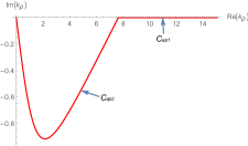
(a) Contour in $k_{\rho}$-plane

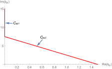
(b) Contour in $k_{\ell z}$-plane

Figure 3.1: Plots of contour used in two level DCIM method ($k_{\ell}=1.5$, $T_{0}=5$).

By taking derivative $D_{\bm{r}}^{\bm{k}}D_{\bm{r}^{\prime}}^{\bm{k}_{0}^{\prime}}$ directly on (3.32), we obtain approximation

$$\frac{D_{\bm{r}}^{\bm{k}}D_{\bm{r}^{\prime}}^{\bm{k}^{\prime}}u_{\ell\ell^{\prime}}(\bm{r},\bm{r}^{\prime})}{\bm{k}!\bm{k}^{\prime}!}\approx\sum\limits_{j=1}^{M}A_{j}^{k_{3}^{\prime}}\frac{D_{\bm{r}}^{\bm{k}}D_{\bm{r}^{\prime}}^{\bm{k}_{0}^{\prime}}h_{0}^{(1)}(k_{\ell}R_{j}^{k_{3}^{\prime}})}{\bm{k}!\bm{k}_{0}^{\prime}!}$$ (3.33)

Note that the approximation (3.29) is independent of $x,y,z,x^{\prime},y^{\prime}$. Approximation (3.33) is expected to maintain the accuracy of the approximation (3.29). Numerical results verify this fact at the end of this section. More importantly, the derivatives on Hankel function with complex coordinates can be calculated by using a recurrence formula.

Define

$$a^{\bm{k}}(\bm{r},\bm{r}^{\prime},k):=\frac{1}{\bm{k}!}D_{\bm{r}}^{\bm{k}}h_{0}^{(1)}(k|\bm{r}-\bm{r}^{\prime}|),\quad b^{\bm{k}}(\bm{r},\bm{r}^{\prime},k)=\frac{1}{\bm{k}!}D_{\bm{r}}^{\bm{k}}\psi,$$ (3.34)

where $\bm{r}^{\prime}=(x^{\prime},y^{\prime},Z^{\prime})$ is a coordinate with complex $z$-coordinate $Z^{\prime}$. Then, we have the following recurrence formula

$$\begin{split}|\bm{k}||\bm{r}-\bm{r}^{\prime}|^{2}a^{\bm{k}}&+2(|\bm{k}|-1)\sum\limits_{i=1}^{3}(\bm{r}-\bm{r}^{\prime})_{i}a^{\bm{k}-\bm{e}_{i}}+(|\bm{k}|+1)\sum\limits_{i=1}^{3}a^{\bm{k}-2\bm{e}_{i}}\\ =&{\rm i}k\Big{(}\sum\limits_{i=1}^{3}(\bm{r}-\bm{r}^{\prime})_{i}b^{\bm{k}-\bm{e}_{i}}+\sum\limits_{i=1}^{2}b^{\bm{k}-2\bm{e}_{i}}\Big{)},\\ |\bm{k}|b^{\bm{k}}=&{\rm i}k\Big{(}\sum\limits_{i=1}^{3}(\bm{r}-\bm{r}^{\prime})_{i}a^{\bm{k}-\bm{e}_{i}}+\sum\limits_{i=1}^{3}a^{\bm{k}-2\bm{e}_{i}}\Big{)}.\end{split}$$ (3.35)

The derivation can be done by simply following the procedure in [22], since the involved derivatives are independent of the complex coordinate $z^{\prime}$. With this recurrence formula, derivatives

$$D_{\bm{r}}^{\bm{k}}D_{\bm{r}^{\prime}}^{\bm{k}_{0}^{\prime}}h_{0}^{(1)}(k_{\ell}R_{j}^{k_{3}^{\prime}})=(-1)^{|\bm{k}_{0}^{\prime}|}D_{\bm{r}}^{\bm{k}+\bm{k}_{0}^{\prime}}h_{0}^{(1)}(k_{\ell}R_{j}^{k_{3}^{\prime}}),$$ (3.36)

can be efficiently calculated.

In the free space TE-FMM, the most time consuming part is the translation from a source box to a target box where a recurrence formula is used to calculate all $O(p^{6})$ derivatives. Note that $D_{\bm{r}}^{\bm{k}}D_{\bm{r}^{\prime}}^{\bm{k}^{\prime}}u_{\ell\ell^{\prime}}^{\uparrow}(\bm{r}_{c}^{l},\bm{r}_{c})$ only depends on the center of the corresponding boxes. More precisely, the density (3.25) approximated by DCIM only depends on the $z$-coordinates of the center of boxes in the source tree. Once the tree structure is fixed, we can pre-compute a table for all complex exponential approximations used for the computation of $D_{\bm{r}}^{\bm{k}}D_{\bm{r}^{\prime}}^{\bm{k}^{\prime}}u_{\ell\ell^{\prime}}^{\uparrow}(\bm{r}_{c}^{l},\bm{r}_{c})$. Assume that the depth of the source tree is $H$, then only $2^{H}(p+1)$ DCIM approximations are needed to be precomputed.

Next, we will give some numerical results to show the accuracy of the two level DCIM and show that taking derivative with respect to $x,y,z,x^{\prime},y^{\prime}$ will not result in an accuracy loss. For this purpose, let us consider the approximation of

$$\Big{(}\frac{\partial}{\partial x}+{\rm i}\frac{\partial}{\partial y}\Big{)}^{s}\Big{(}\frac{\partial}{\partial z}\Big{)}^{k_{3}}\Big{(}\frac{\partial}{\partial z^{\prime}}\Big{)}^{k_{3}^{\prime}}\frac{u_{11}^{\uparrow}(\bm{r},\bm{r}^{\prime})}{s!k_{3}!k_{3}^{\prime}!},$$ (3.37)

for three layers case with $k_{0}=0.8$, $k_{1}=1.5$, $k_{2}=2.0$, $d=2.0$. In the two level DCIM approximation, we set $T_{0}=\sqrt{\Big{(}\frac{k_{2}+0.8}{k_{1}}\Big{)}^{2}-1},T_{1}=10$ and use $101$ sample points in each level.

	$(k_{3},k_{3}^{\prime},s)$	direct quadrature	DCIM	error
$\bm{r}=(0.5,1.0,-0.5)$ $\bm{r}^{\prime}=(0.3,1.3,-0.5)$	(0, 0, 0)	0.0636386627264339	0.063638662478093	2.4834e-10
	(3, 4, 0)	0.00474777580070183	0.004747777003526	-1.2028e-09
	(8, 8, 0)	-7.40635683599036e-10	-7.406632552555640e-10	2.7572e-14
	(0, 0, 4)	-1.77276908208051e-06	-1.772752691103600e-06	-1.6391e-11
	(0, 0, 8)	1.61980348471514e-11	1.619802703109298e-11	7.8161e-18
$\bm{r}=(0.6,0.3,-1.2)$ $\bm{r}^{\prime}=(0.5,1.0,-0.5)$	(0, 0, 0)	0.0470021533117637	0.047002199376864	-4.6065e-08
	(3, 4, 0)	0.00185695910047338	0.001856957782404	1.3181e-09
	(8, 8, 0)	5.85835080649916e-09	5.858364813170763e-09	-1.4007e-14
	(0, 0, 4)	-1.71372127668556e-05	-1.713524114661759e-05	-1.9716e-9
	(0, 0, 8)	-1.26729956194435e-07	-1.267386149809553e-07	8.6588e-12

Table 3.1: Numerical results of $(k_{3},k_{3}^{\prime},s)-$derivatives in (3.37) (real parts).

	$(k_{3},k_{3}^{\prime},s)$	direct quadrature	DCIM	error
$\bm{r}=(0.5,1.0,-0.5)$ $\bm{r}^{\prime}=(0.3,1.3,-0.5)$	(0, 0, 0)	0.00236214962912961	0.002362151697708	-2.0686e-09
	(3, 4, 0)	-0.00126663970537548	- 0.001266638701878	-1.0035e-09
	(8, 8, 0)	1.3083718652325e-06	1.308371795385077e-06	6.9847e-14
	(0, 0, 4)	-1.50190394931086e-06	- 1.501883557929564e-06	-2.0391e-11
	(0, 0, 8)	-2.87922306729206e-13	- 2.878701763048925e-13	-5.2130e-17
$\bm{r}=(0.6,0.3,-1.2)$ $\bm{r}^{\prime}=(0.5,1.0,-0.5)$	(0, 0, 0)	-0.0655662374392812	- 0.065566216753017	-2.069e-08
	(3, 4, 0)	-0.00407200441147604	- 0.004072001032057	-3.3794e-09
	(8, 8, 0)	-5.8052078071366e-05	- 5.805409125522990e-05	2.0132e-09
	(0, 0, 4)	0.000103591338132027	1.035831449609178e-04	8.1932e-09
	(0, 0, 8)	5.90666673167792e-08	5.907018897856176e-08	-3.5217e-12

Table 3.2: Numerical results of $(k_{3},k_{3}^{\prime},s)-$derivatives in (3.37) (imaginary parts).

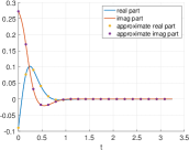
(a) $k_{3}^{\prime}=0$

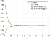
(b) $k_{3}^{\prime}=4$

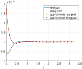
(c) $k_{3}^{\prime}=8$

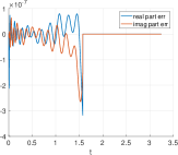
(d) $k_{3}^{\prime}=0$

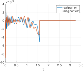
(e) $k_{3}^{\prime}=4$

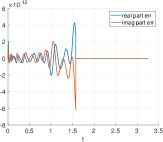
(f) $k_{3}^{\prime}=8$

Figure 3.2: Plots of two level DCIM approximation for $\Theta_{11}^{k_{3}^{\prime}}(k_{\rho},-0.5)$.

Approximations of $\Theta_{11}^{k_{3}^{\prime}}(k_{\rho},-0.5)$ with $z_{min}=-1.5$ and corresponding errors for different order of derivatives are depicted in Fig. 3.2. Numerical results obtained by direct quadrature with contour deformation and DCIM approximation are compared in Table 3.1-3.2. A large number of Gauss points is used for the quadrature calculation so a machine accuracy is obtained to be used as reference values. The numerical results presented in Table 3.1-3.2 show that DCIM can produce approximation with high accuracy even for high order derivatives. Taking derivative with respect to $x,y,z$ has no degeneracy on the accuracy. Since derivatives with respect to $x^{\prime},y^{\prime}$ are just a sign change of that with respect to $x,y$, it also shows that taking derivative with respect to $x^{\prime},y^{\prime}$ will not degenerate the accuracy neither.

Now we can present two algorithms for the computation of general component (3.17) and total interaction (3.15), respectively.

Algorithm 1 TEFMM-I for general component (3.17)

Generate an adaptive hierarchical tree structure and precompute tables.

Upward pass:

for $l=H\to 0$ do

     for all boxes $j$ on source tree level $l$  do

         if $j$ is a leaf node then

              form the free-space TE using Eq. (3.19).

         else

              form the free-space TE by merging children’s expansions using the free-space center shift translation operator (3.9).

         end if

     end for

end for

Downward pass:

for $l=1\to H$ do

     for all boxes $j$ on target tree level $l$  do

         shift the TE of $j$’s parent to $j$ itself using the free-space translation operator (3.14).

         collect interaction list contribution using the source box to target box translation operator in Eq. (3.21) with precomputed table for (3.29) and recurrence formula (3.35).

     end for

end for

Evaluate Local Expansions:

for each leaf node (childless box) do

     evaluate the local expansion at each particle location.

end for

Local Direct Interactions:

for $i=1\to N$  do

     compute Eq. (3.17) of target particle $i$ in the neighboring boxes using precomputed table of $u_{\ell\ell^{\prime}}^{\uparrow}(\bm{r},\bm{r}^{\prime})$.

end for

Algorithm 2 Taylor expansion based heterogeneous 3-D FMM for (3.15)

for $\ell=0\to L$ do

     for $\ell^{\prime}=0\to L$  do

         if $\ell=\ell^{\prime}$ then

              use free space FMM to compute $\Phi_{\ell}^{free}$.

         end if

         if $\ell=0$ then

              use Algorithm 1 to compute $\Phi_{0\ell^{\prime}}^{\uparrow}$.

         else

              if $\ell=L$ then

                  use Algorithm 1 to compute $\Phi_{L\ell^{\prime}}^{\downarrow}$.

              else

                  use Algorithm 1 to compute $\Phi_{\ell\ell^{\prime}}^{\uparrow}$.

                  use Algorithm 1 to compute $\Phi_{\ell\ell^{\prime}}^{\downarrow}$.

              end if

         end if

     end for

end for

4 Second Taylor-Expansion based FMM in multi-layered media

As discussed in the last section, Taylor expansion based FMM in multi-layered media depends on an efficient algorithm for the calculation of corresponding Green’s function and its derivatives. The algorithm using discrete complex image and recurrence formula has good efficiency. However, discrete complex image approximation may suffer stability problem in the calculation of high order derivatives. Since the Green’s function in multi-layered media has a symmetry in the $x-y$ plane, it is worthy to maintain this symmetry. For this purpose, we use notation $\mathcal{H}_{k}(\bm{r},\bm{r}^{\prime})=h_{0}^{(1)}(k|\bm{r}-\bm{r}^{\prime}|)$ and introduce differential operators

$$\begin{split}\mathscr{D}_{nm}^{s}=&\Big{(}\frac{\partial}{\partial x}-{\rm i}\frac{\partial}{\partial y}\Big{)}^{s}\Big{(}\frac{\partial}{\partial x}+{\rm i}\frac{\partial}{\partial y}\Big{)}^{m-{s}}\Big{(}\frac{\partial}{\partial z}\Big{)}^{n-m},\\ \widehat{\mathscr{D}}_{nm}^{s}=&\Big{(}\frac{\partial}{\partial x^{\prime}}-{\rm i}\frac{\partial}{\partial y^{\prime}}\Big{)}^{s}\Big{(}\frac{\partial}{\partial x^{\prime}}+{\rm i}\frac{\partial}{\partial y^{\prime}}\Big{)}^{m-s}\Big{(}\frac{\partial}{\partial z^{\prime}}\Big{)}^{n-m}.\end{split}$$ (4.1)

4.1 Free space

We start with rearranging TE of $h_{0}^{(1)}(k|\bm{r}-\bm{r}^{\prime}|)$ by using operators defined in (4.1).

Theorem 4.1.

Suppose $|\bm{r}^{\prime}|\leq a$ for a given small radius $a$, then the Taylor expansion of $h_{0}^{(1)}(k|\bm{r}-\bm{r}^{\prime}|)$ at origin with respect to $\bm{r}^{\prime}$ is

$$h_{0}^{(1)}(k|\bm{r}-\bm{r}^{\prime}|)=\sum_{n=0}^{\infty}\sum_{m=0}^{n}\sum_{s=0}^{m}\tilde{\alpha}_{nm}^{s}(\bm{r}^{\prime})\frac{\widehat{\mathscr{D}}_{nm}^{s}\mathcal{H}_{k}(\bm{r},\bm{0})}{2^{m}(n-m)!s!(m-s)!},$$ (4.2)

where

$$\quad\tilde{\alpha}_{nm}^{s}(\bm{r}^{\prime})=(x^{\prime}+{\rm i}y^{\prime})^{s}(x^{\prime}-{\rm i}y^{\prime})^{m-s}(z^{\prime})^{n-m}.$$ (4.3)

Proof.

Denote the spherical coordinates of ${\bm{r}}^{\prime}$ and ${\bm{r}}$ as $(\rho,\alpha,\beta)$ and $(r,\theta,\varphi)$, repsectively. Applying Taylor expansion on $h_{0}^{(1)}(k|{\bm{r}}-{\bm{r}}^{\prime}|)$ with respect to $\bm{r}^{\prime}=(x^{\prime},y^{\prime},z^{\prime})$ at the origin and changing the derivative with respect to $(x,y,z)$, we have

$$\begin{split}h_{0}^{(1)}(k|{\bm{r}}-{\bm{r}}^{\prime}|)=&\mathcal{H}_{k}({\bm{r}},\bm{0})+\sum_{n=1}^{\infty}\frac{(-1)^{n}}{n!}\left(x^{\prime}\frac{\partial}{\partial x}+y^{\prime}\frac{\partial}{\partial y}+z^{\prime}\frac{\partial}{\partial z}\right)^{n}\mathcal{H}_{k}({\bm{r}},\bm{0})\\ =&\mathcal{H}_{k}({\bm{r}},\bm{0})+\sum_{n=1}^{\infty}\frac{(-1)^{n}\rho^{n}}{n!}\sum_{m=0}^{n}\binom{n}{m}\sin^{m}\alpha\left(\cos{\beta}\frac{\partial}{\partial x}+\sin{\beta}\frac{\partial}{\partial y}\right)^{m}\\ &\qquad\qquad\qquad\qquad\qquad\qquad\qquad\times\cos^{n-m}\alpha\left(\frac{\partial}{\partial z}\right)^{n-m}\mathcal{H}_{k}({\bm{r}},\bm{0}).\end{split}$$ (4.4)

Notice that for any function $f(z),z\in\mathbb{C}$, we have

$$\left(\cos{\beta}\frac{\partial}{\partial x}+\sin{\beta}\frac{\partial}{\partial y}\right)f=\frac{1}{2}\Big{[}e^{{\rm i}\beta}\left(\frac{\partial}{\partial x}-{\rm i}\frac{\partial}{\partial y}\right)+e^{-{\rm i}\beta}\left(\frac{\partial}{\partial x}+{\rm i}\frac{\partial}{\partial y}\right)\Big{]}f.$$

Therefore, we can rewrite Eq. (4.4) as

$$\begin{split}h_{0}^{(1)}(k|{\bm{r}}-{\bm{r}}^{\prime}|)=&\mathcal{H}_{k}({\bm{r}},\bm{0})+\sum_{n=1}^{\infty}\sum_{m=0}^{n}\frac{(-1)^{n}\rho^{n}\sin^{m}\alpha\cos^{n-m}\alpha}{2^{m}(n-m)!}\\ &\qquad\qquad\qquad\qquad\times\sum_{s=0}^{m}\frac{e^{-{\rm i}(m-s)\beta}e^{{\rm i}s\beta}}{s!(m-s)!}\mathscr{D}_{nm}^{s}\mathcal{H}_{k}({\bm{r}},\bm{0})\\ =&\mathcal{H}_{k}({\bm{r}},\bm{0})+\sum_{n=1}^{\infty}\sum_{m=0}^{n}\sum_{s=0}^{m}\tilde{\alpha}_{nm}^{s}(\bm{r}^{\prime})\frac{(-1)^{n}\mathscr{D}_{nm}^{s}\mathcal{H}_{k}({\bm{r}},\bm{0})}{2^{m}(n-m)!s!(m-s)!},\end{split}$$ (4.5)

where

$$\tilde{\alpha}_{nm}^{s}(\bm{r}^{\prime})=\rho^{n}e^{{\rm i}s\beta}e^{-{\rm i}(m-s)\beta}\sin^{m}\alpha\cos^{n-m}\alpha=(x^{\prime}+{\rm i}y^{\prime})^{s}(x^{\prime}-{\rm i}y^{\prime})^{m-s}(z^{\prime})^{n-m}.$$ (4.6)

We finish the proof by using the fact $(-1)^{n}\mathscr{D}_{nm}^{s}\mathcal{H}_{k}({\bm{r}},\bm{0})=\widehat{\mathscr{D}}_{nm}^{s}\mathcal{H}_{k}({\bm{r}},\bm{0})$ in (4.5). ∎

Remark 4.1.

The notation $\mathcal{H}_{k}({\bm{r}},\bm{r}^{\prime})$ is used to clearly show that the derivatives $\mathscr{D}_{nm}^{s}h_{0}^{(1)}(k|{\bm{r}}-\bm{r}^{\prime}|)$ and $\widehat{\mathscr{D}}_{nm}^{s}h_{0}^{(1)}(k|{\bm{r}}-\bm{r}^{\prime}|)$ are not just depend on $|\bm{r}-\bm{r}^{\prime}|$ but are functions of $(\bm{r},\bm{r}^{\prime})$.

Corollary 4.1.

Suppose $|\bm{r}|\leq a$ for a given small radius $a$, then the Taylor expansion of $h_{0}^{(1)}(k|\bm{r}-\bm{r}^{\prime}|)$ at the origin with respect to $\bm{r}$ is

$$h_{0}^{(1)}(k|\bm{r}-\bm{r}^{\prime}|)=\sum_{n=0}^{\infty}\sum_{m=0}^{n}\sum_{s=0}^{m}{\beta}_{nm}^{s}\tilde{\alpha}_{nm}^{s}(\bm{r})$$ (4.7)

where

$${\beta}_{nm}^{s}=\frac{\mathscr{D}_{nm}^{s}\mathcal{H}_{k}(\bm{0},\bm{r}^{\prime})}{2^{m}(n-m)!s!(m-s)!}.$$ (4.8)

With Taylor expansions given in (4.2) and (4.7), we can have the second Taylor expansion based FMM which uses the following expansions:

• Taylor expansion (TE) in a source box centered at $\bm{r}_{c}$:

  $$\sum\limits_{j\in J_{m}}q_{j}h_{0}^{(1)}(k|\bm{r}-\bm{r}_{j}|)\approx\sum_{n=0}^{p}\sum_{m=0}^{n}\sum_{s=0}^{m}{\alpha}_{nm}^{s}\frac{\widehat{\mathscr{D}}_{nm}^{s}\mathcal{H}_{k}(\bm{r},\bm{r}_{c})}{2^{m}(n-m)!s!(m-s)!},$$ (4.9)

  where

  $${\alpha}_{nm}^{s}=\sum\limits_{j\in J_{m}}q_{j}\tilde{\alpha}_{nm}^{s}(\bm{r}_{j}-\bm{r}_{c}).$$ (4.10)

• Taylor expansion (TE) in a target box centered at $\bm{r}_{c}^{l}$:

  $$\sum\limits_{j\in J_{m}}q_{j}h_{0}^{(1)}(k|\bm{r}-\bm{r}_{j}|)\approx\sum_{n=0}^{p}\sum_{m=0}^{n}\sum_{s=0}^{m}{\beta}_{nm}^{s}\tilde{\alpha}_{nm}^{s}(\bm{r}-\bm{r}_{c}^{l}),$$ (4.11)

  where

  $${\beta}_{nm}^{s}=\sum\limits_{j\in J_{m}}\frac{q_{j}\mathscr{D}_{nm}^{s}\mathcal{H}_{k}(\bm{r}_{c}^{l},\bm{r}_{j})}{2^{m}(n-m)!s!(m-s)!}.$$ (4.12)

The translation operators used in the FMM algorithm can be derived similarly as in the conventional way. Firstly, by applying Taylor expansion (4.9) in (4.12) and using the fact $\mathcal{H}_{k}(\bm{r}_{c}^{l},\bm{r}_{j})=h_{0}^{(1)}(k|\bm{r}^{l}_{c}-\bm{r}_{j}|)$, we have

$$\begin{split}{\beta}_{nm}^{s}=&\frac{1}{2^{m}(n-m)!s!(m-s)!}\mathscr{D}_{nm}^{s}\sum_{n^{\prime}=0}^{p}\sum_{m^{\prime}=0}^{n^{\prime}}\sum_{s^{\prime}=0}^{m^{\prime}}{\alpha}_{n^{\prime}m^{\prime}}^{s^{\prime}}\frac{\widehat{\mathscr{D}}_{n^{\prime}m^{\prime}}^{s^{\prime}}\mathcal{H}_{k}(\bm{r}_{c}^{l},\bm{r}_{c})}{2^{m^{\prime}}(n^{\prime}-m^{\prime})!s^{\prime}!(m^{\prime}-s^{\prime})!}\\ =&\sum_{n^{\prime}=0}^{p}\sum_{m^{\prime}=0}^{n^{\prime}}\sum_{s^{\prime}=0}^{m^{\prime}}{\alpha}_{n^{\prime}m^{\prime}}^{s^{\prime}}\frac{\mathscr{D}_{nm}^{s}\widehat{\mathscr{D}}_{n^{\prime}m^{\prime}}^{s^{\prime}}\mathcal{H}_{k}(\bm{r}_{c}^{l},\bm{r}_{c})}{2^{m+m^{\prime}}(n-m)!s!(m-s)!(n^{\prime}-m^{\prime})!s^{\prime}!(m^{\prime}-s^{\prime})!}.\end{split}$$

Therefore, the translation operator from TE in a source box centered at $\bm{r}_{c}$ to TE in a target box centered at $\bm{r}_{c}^{l}$ is given by

$${\beta}_{nm}^{s}=\sum_{n^{\prime}=0}^{p}\sum_{m^{\prime}=0}^{n^{\prime}}\sum_{s^{\prime}=0}^{m^{\prime}}{\alpha}_{n^{\prime}m^{\prime}}^{s^{\prime}}L_{nms}^{n^{\prime}m^{\prime}s^{\prime}},$$ (4.13)

where

$$L_{nms}^{n^{\prime}m^{\prime}s^{\prime}}=\frac{\mathscr{D}_{nm}^{s}\widehat{\mathscr{D}}_{n^{\prime}m^{\prime}}^{s^{\prime}}\mathcal{H}_{k}(\bm{r}_{c}^{l},\bm{r}_{c})}{2^{m+m^{\prime}}(n-m)!s!(m-s)!(n^{\prime}-m^{\prime})!s^{\prime}!(m^{\prime}-s^{\prime})!}.$$ (4.14)

Denote the coefficients of TE in the source box centered at $\bm{r}_{c}^{\prime}$ by

$${\gamma}_{nm}^{s}=\sum\limits_{j=1}^{N}q_{j}\tilde{\alpha}_{nm}^{s}(\bm{r}_{j}-\bm{r}_{c}^{\prime}).$$

Direct calculation gives

$$\begin{split}&[(x_{j}-x_{c}^{\prime})+{\rm i}(y_{j}-y_{c}^{\prime})]^{s}[(x_{j}-x_{c}^{\prime})-{\rm i}(y_{j}-y_{c}^{\prime})]^{m-s}(z_{j}-z_{c}^{\prime})^{n-m}\\ =&\sum\limits_{s^{\prime}=0}^{s}\sum\limits_{m^{\prime}=0}^{m-s}\sum\limits_{n^{\prime}=0}^{n-m}B_{nms}^{n^{\prime}m^{\prime}s^{\prime}}[(x_{j}-x_{c})+{\rm i}(y_{j}-y_{c})]^{s^{\prime}}[(x_{j}-x_{c})-{\rm i}(y_{j}-y_{c})]^{m^{\prime}}(z_{j}-z_{c})^{n^{\prime}}\end{split}$$ (4.15)

where

$$\begin{split}B_{nms}^{n^{\prime}m^{\prime}s^{\prime}}=&\frac{s!(m-s)!(n-m)![(x_{c}-x_{c}^{\prime})+{\rm i}(y_{c}-y_{c}^{\prime})]^{s-s^{\prime}}}{s^{\prime}!(s-s^{\prime})!m^{\prime}!(m-s-m^{\prime})!n^{\prime}!(n-m-n^{\prime})!}\\ &\times[(x_{c}-x_{c}^{\prime})-{\rm i}(y_{c}-y_{c}^{\prime})]^{m-s-m^{\prime}}(z_{c}-z_{c}^{\prime})^{n-m-n^{\prime}}.\end{split}$$ (4.16)

Therefore,

$$\tilde{\alpha}_{nm}^{s}(\bm{r}_{j}-\bm{r}_{c}^{\prime})=\sum\limits_{s^{\prime}=0}^{s}\sum\limits_{m^{\prime}=0}^{m-s}\sum\limits_{n^{\prime}=0}^{n-m}B_{nms}^{n^{\prime}m^{\prime}s^{\prime}}\tilde{\alpha}_{n^{\prime}+m^{\prime}+s^{\prime},m^{\prime}+s^{\prime}}^{s^{\prime}}(\bm{r}_{j}-\bm{r}_{c}),$$ (4.17)

which implies that the translation operator from TE in a source box centered at $\bm{r}_{c}$ to TE in another source box centered at $\bm{r}_{c}^{\prime}$ has the form

$$\gamma_{nm}^{s}=\sum\limits_{s^{\prime}=0}^{s}\sum\limits_{m^{\prime}=0}^{m-s}\sum\limits_{n^{\prime}=0}^{n-m}B_{nms}^{n^{\prime}m^{\prime}s^{\prime}}{\alpha}_{n^{\prime}+m^{\prime}+s^{\prime},m^{\prime}+s^{\prime}}^{s^{\prime}}.$$ (4.18)

Let

$${\lambda}_{nm}^{s}=\sum\limits_{j\in J_{m}}\frac{q_{j}\mathscr{D}_{nm}^{s}\mathcal{H}_{k}(\tilde{\bm{r}}_{c}^{l},\bm{r}_{j})}{2^{m}(n-m)!s!(m-s)!},$$ (4.19)

be the coefficients of TE in a target box centered at $\tilde{\bm{r}}_{c}^{l}$. By applying Taylor expansion at $\bm{r}_{c}^{l}$ we obtain

$$\begin{split}{\lambda}_{nm}^{s}=&\frac{1}{2^{m}(n-m)!s!(m-s)!}{\mathscr{D}}_{nm}^{s}\sum\limits_{j\in J_{m}}q_{j}h_{0}^{(1)}(k|\tilde{\bm{r}}_{c}^{l}-\bm{r}_{j}|)\\ \approx&\frac{1}{2^{m}(n-m)!s!(m-s)!}\sum_{n^{\prime}=0}^{p}\sum_{m^{\prime}=0}^{n^{\prime}}\sum_{s^{\prime}=0}^{m^{\prime}}{\beta}_{n^{\prime}m^{\prime}}^{s^{\prime}}{\mathscr{D}}_{nm}^{s}\tilde{\alpha}_{n^{\prime}m^{\prime}}^{s^{\prime}}(\tilde{\bm{r}}_{c}^{l}-\bm{r}_{c}^{l}).\end{split}$$ (4.20)

Note that

$$\begin{split}&\Big{(}\frac{\partial}{\partial\tilde{x}_{c}^{l}}-{\rm i}\frac{\partial}{\partial\tilde{y}_{c}^{l}}\Big{)}^{s}\Big{(}\frac{\partial}{\partial\tilde{x}_{c}^{l}}+{\rm i}\frac{\partial}{\partial\tilde{y}_{c}^{l}}\Big{)}^{m-s}[(\tilde{x}_{c}^{l}-x_{c}^{l})+{\rm i}(\tilde{y}_{c}^{l}-y_{c}^{l})]^{s^{\prime}}[(\tilde{x}_{c}^{l}-x_{c}^{l})-{\rm i}(\tilde{y}_{c}^{l}-y_{c}^{l})]^{m^{\prime}-s^{\prime}}\\ =&\begin{cases}\displaystyle 0,\quad m-s>m^{\prime}-s^{\prime}\;\;\mathrm{or}\;\;s>s^{\prime},\\[6.0pt] \displaystyle\frac{2^{m}s^{\prime}!(m^{\prime}-s^{\prime})![(\tilde{x}_{c}^{l}-x_{c}^{l})+{\rm i}(\tilde{y}_{c}^{l}-y_{c}^{l})]^{s^{\prime}-s}}{(s^{\prime}-s)!(m^{\prime}-s^{\prime}-m+s)!}[(\tilde{x}_{c}^{l}-x_{c}^{l})-{\rm i}(\tilde{y}_{c}^{l}-y_{c}^{l})]^{m^{\prime}-s^{\prime}-m+s},\quad\mathrm{otherwise},\end{cases}\\ &\Big{(}\frac{\partial}{\partial\tilde{z}_{c}^{l}}\Big{)}^{n-m}(\tilde{z}_{c}^{l}-z_{c}^{l})^{n^{\prime}-m^{\prime}}=\begin{cases}\displaystyle 0,\quad\mathrm{if}\;n-m>n^{\prime}-m^{\prime},\\ \displaystyle\frac{(n^{\prime}-m^{\prime})!}{(n^{\prime}-m^{\prime}-(n-m))!}(\tilde{z}_{c}^{l}-z_{c}^{l})^{n^{\prime}-m^{\prime}-n+m},\;\mathrm{otherwise}.\\ \end{cases}\end{split}$$

Therefore,

$${\mathscr{D}}_{nm}^{s}\tilde{\alpha}_{n^{\prime}m^{\prime}}^{s^{\prime}}(\tilde{\bm{r}}_{c}^{l}-\bm{r}_{c}^{l})=\begin{cases}\displaystyle 0,\quad\mathrm{if}\;\;m-s>m^{\prime}-s^{\prime}\;\;\mathrm{or}\;\;s>s^{\prime}\;\;\mathrm{or}\;\;\;n-m>n^{\prime}-m^{\prime};\\[10.0pt] \displaystyle 2^{m}C_{nms}^{n^{\prime}m^{\prime}s^{\prime}}\tilde{\alpha}_{n^{\prime}-n,m^{\prime}-m}^{s^{\prime}-s}(\tilde{\bm{r}}_{c}^{l}-\bm{r}_{c}^{l}),\quad\mathrm{otherwise},\end{cases}$$ (4.21)

where

$$C_{nms}^{n^{\prime}m^{\prime}s^{\prime}}=\frac{(m^{\prime}-s^{\prime})!s^{\prime}!(n^{\prime}-m^{\prime})!}{(m^{\prime}-s^{\prime}-m+s)!(s^{\prime}-s)!(n^{\prime}-m^{\prime}-(n-m))!}.$$

Substituting (4.21) into (4.20) gives the translation operator from TE in a target box centered at $\bm{r}_{c}^{l}$ to TE in another target box centered at $\tilde{\bm{r}}_{c}^{l}$

$${\lambda}_{nm}^{s}=\sum\limits_{n^{\prime}=n}^{p}\sum\limits_{m^{\prime}=m}^{m+n^{\prime}-n}\sum_{s^{\prime}=s}^{s+m^{\prime}-m}\beta_{n^{\prime}m^{\prime}}^{s^{\prime}}\frac{C_{nms}^{n^{\prime}m^{\prime}s^{\prime}}\tilde{\alpha}_{n^{\prime}-n,m^{\prime}-m}^{s^{\prime}-s}(\tilde{\bm{r}}_{c}^{l}-\bm{r}_{c}^{l})}{(n-m)!s!(m-s)!}.$$ (4.22)

To ensure the efficiency of this algorithm, a fast algorithm is needed for the calculation of derivatives $\mathscr{D}_{nm}^{s}\mathcal{H}_{k}(\bm{r},\bm{r}^{\prime})$ and $\mathscr{D}_{nm}^{s}\widehat{\mathscr{D}}_{n^{\prime}m^{\prime}}^{s^{\prime}}\mathcal{H}_{k}(\bm{r},\bm{r}^{\prime})$ which are used in the computation of coefficients (4.12) and translation operators (4.14). A recurrence formula can be derived from the following result (cf.[36]). Define

$$\Omega_{n}^{m}(\bm{r})=h_{n}^{(1)}(k|\bm{r}|)Y_{n}^{m}(\theta,\phi),\quad\mathscr{D}^{\pm}=\frac{1}{k}\Big{(}\frac{\partial}{\partial x}\pm{\rm i}\frac{\partial}{\partial y}\Big{)},\quad\mathscr{D}^{0}=-\frac{1}{k}\frac{\partial}{\partial z},$$ (4.23)

where

$$Y_{n}^{m}(\theta,\phi)=(-1)^{m}\sqrt{\frac{2n+1}{4\pi}\frac{(n-m)!}{(n+m)!}}P_{l}^{m}(\cos\theta)e^{{\rm i}m\phi},$$ (4.24)

is the spherical harmonics.

Theorem 4.2.

For $0\leq|m|\leq n$,

$$\begin{split}&\mathscr{D}^{+}\Omega_{n}^{m}=A_{nm}^{+}\Omega_{n+1}^{m+1}+B_{nm}^{+}\Omega_{n-1}^{m+1},\\ &\mathscr{D}^{-}\Omega_{n}^{m}=A_{nm}^{-}\Omega_{n+1}^{m-1}+B_{nm}^{-}\Omega_{n-1}^{m-1},\\ &\mathscr{D}^{0}\Omega_{n}^{m}=A_{nm}^{0}\Omega_{n+1}^{m}+B_{nm}^{0}\Omega_{n-1}^{m}.\end{split}$$ (4.25)

where

$$\begin{split}&A_{nm}^{+}=\sqrt{\frac{(n+m+2)(n+m+1)}{(2n+1)(2n+3)}},\quad B_{nm}^{+}=\sqrt{\frac{(n-m)(n-m-1)}{4n^{2}-1}},\\ &A_{nm}^{-}=-\sqrt{\frac{(n-m+2)(n-m+1)}{(2n+1)(2n+3)}},\quad B_{nm}^{-}=-\sqrt{\frac{(n+m)(n+m-1)}{4n^{2}-1}},\\ &A_{nm}^{0}=-\sqrt{\frac{(n+1)^{2}-m^{2}}{(2n+1)(2n+3)}},\quad B_{nm}^{0}=\sqrt{\frac{n^{2}-m^{2}}{4n^{2}-1}}.\end{split}$$

In particular, for $n\geq 0$

$$\mathscr{D}^{0}\Omega_{n}^{\pm n}=\frac{1}{\sqrt{2n+3}}\Omega_{n+1}^{\pm n}.$$ (4.26)

From the theorem 4.2, the high order derivatives can be expressed as

$$\{(\mathscr{D}^{+})^{s},(\mathscr{D}^{-})^{s},(\mathscr{D}^{0})^{s}\}\Omega_{n}^{m}=\sum\limits_{r=0}^{s}\big{\{}{C}_{rs}^{+}\Omega_{n-s+2r}^{m+s},{C}_{rs}^{-}\Omega_{n-s+2r}^{m-s},C_{rs}^{0}\Omega_{n-s+2r}^{m}\big{\}},$$

where the coefficients $\{{C}_{rs}^{+}\},\{C_{rs}^{-}\},\{{C}_{rs}^{0}\}$ have a recurrence formula

$$\begin{split}&C_{rs}^{+}=\begin{cases}\displaystyle 0,&n-s+2r<m+s,\\[5.0pt] \displaystyle B_{n-s+1,m+s-1}^{+}C_{0,s-1}^{+},&r=0,\\[5.0pt] \displaystyle A_{n+s-1,m+s-1}^{+}C_{s-1,s-1}^{+},&r=s,\\[5.0pt] \displaystyle A_{n-s+2r-1,m+s-1}^{+}C_{r-1,s-1}^{+}+B_{n-s+2r+1,m+s-1}^{+}C_{r,s-1}^{+},&0<r<s,\end{cases}\\ &C_{rs}^{-}=\begin{cases}\displaystyle 0,&n-s+2r<|m-s|,\\[5.0pt] \displaystyle B_{n-s+1,m-s+1}^{-}C_{0,s-1}^{-},&r=0,\\[5.0pt] \displaystyle A_{n+s-1,m-s+1}^{-}C_{s-1,s-1}^{-},&r=s,\\[5.0pt] \displaystyle A_{n-s+2r-1,m-s+1}^{-}C_{r-1,s-1}^{-}+B_{n-s+2r+1,m-s+1}^{-}C_{r,s-1}^{-},&0<r<s,\end{cases}\\ &{C}_{rs}^{0}=\begin{cases}\displaystyle 0,&n-s+2r<m,\\[5.0pt] \displaystyle B_{n-s+1,m}^{0}C_{0,s-1}^{0},&r=0,\\[5.0pt] \displaystyle A_{n+s-1,m}^{0}C_{s-1,s-1}^{0},&r=s,\\[5.0pt] \displaystyle A_{n-(s-2r)-1,m}^{0}C_{r-1,s-1}^{0}+B_{n-(s-2r)+1,m}^{0}C_{r,s-1}^{0},&0<r<s,\end{cases}\end{split}$$

with initial values

$$C_{00}^{+}=C_{00}^{-}={C}_{00}^{0}=1.$$

Therefore,

$$\begin{split}\mathscr{D}_{nm}^{s}\mathcal{H}_{k}(\bm{r},\bm{r}^{\prime})=&\Big{(}\frac{-1}{k}\Big{)}^{n}\sqrt{\frac{1}{4\pi}}(\mathscr{D}^{-})^{s}(\mathscr{D}^{+})^{m-s}(\mathscr{D}^{0})^{n-m}\Omega_{0}^{0}(\bm{r}-\bm{r}^{\prime})\\ =&\Big{(}\frac{-1}{k}\Big{)}^{n}\sqrt{\frac{1}{4\pi}}\sum\limits_{n^{\prime}=0}^{n-m}\sum\limits_{m^{\prime}=0}^{m-s}\sum\limits_{s^{\prime}=0}^{s}C_{n^{\prime}m^{\prime}}^{s^{\prime}}\Omega_{2(n^{\prime}+m^{\prime}+s^{\prime})-n}^{m-2s}(\bm{r}-\bm{r}^{\prime}),\end{split}$$ (4.27)

where the coefficients $\{C_{n^{\prime}m^{\prime}}^{s^{\prime}}\}$ can be computed using coefficients $\{{C}_{rs}^{+}\},\{C_{rs}^{-}\},\{{C}_{rs}^{0}\}$. This formula is also used for the calculation of $\mathscr{D}_{nm}^{s}\widehat{\mathscr{D}}_{n^{\prime}m^{\prime}}^{s^{\prime}}\mathcal{H}_{k}(\bm{r},\bm{r}^{\prime})=(-1)^{n^{\prime}}\mathscr{D}_{n+n^{\prime},m+m^{\prime}}^{s+s^{\prime}}\mathcal{H}_{k}(\bm{r},\bm{r}^{\prime})$.

4.2 Multi-layer media

Consider the calculation of interactions given by (3.15) with the setting presented in the last section. We only need to focus on a general component given by (3.17). According to (4.9)-(4.12), the TE-FMM for (3.17) will use Taylor expansions

$$\Phi_{\ell\ell^{\prime}}^{b\uparrow}(\bm{r}_{\ell i})=\sum_{n=0}^{\infty}\sum_{m=0}^{n}\sum_{s=0}^{m}{\alpha}_{nm}^{s}\frac{\widehat{\mathscr{D}}_{nm}^{s}u_{\ell\ell^{\prime}}^{\uparrow}(\bm{r}_{\ell i},\bm{r}_{c})}{2^{m}(n-m)!s!(m-s)!},\quad{\alpha}_{nm}^{s}=\sum\limits_{j\in J_{m}}Q_{\ell^{\prime}j}\tilde{\alpha}_{nm}^{s}(\bm{r}_{\ell^{\prime}j}-\bm{r}_{c}),$$ (4.28)

in a source box centered at $\bm{r}_{c}=(x_{c},y_{c},z_{c})$ and

$$\Phi_{\ell\ell^{\prime}}^{b\uparrow}(\bm{r}_{\ell i})=\sum_{n=0}^{p}\sum_{m=0}^{n}\sum_{s=0}^{m}{\beta}_{nm}^{s}\tilde{\alpha}_{nm}^{s}(\bm{r}_{\ell i}-\bm{r}_{c}^{l}),\quad{\beta}_{nm}^{s}=\sum\limits_{j\in J_{m}}\frac{Q_{\ell^{\prime}j}\mathscr{D}_{nm}^{s}u_{\ell\ell^{\prime}}^{\uparrow}(\bm{r}_{c}^{l},\bm{r}_{\ell^{\prime}j})}{2^{m}(n-m)!s!(m-s)!},$$ (4.29)

in a target box centered at $\bm{r}_{c}^{l}=(x_{c}^{l},y_{c}^{l},z_{c}^{l})$, respectively.

Applying TE (4.28) in the expression of the coefficients $\beta_{nm}^{s}$ in (4.29), we obtain

$${\beta}_{nm}^{s}\approx\sum_{n^{\prime}=0}^{p}\sum_{m^{\prime}=0}^{n^{\prime}}\sum_{s^{\prime}=0}^{m^{\prime}}{\alpha}_{n^{\prime}m^{\prime}}^{s^{\prime}}\frac{\mathscr{D}_{nm}^{s}\widehat{\mathscr{D}}_{n^{\prime},m^{\prime}}^{s^{\prime}}u_{\ell\ell^{\prime}}^{\uparrow}(\bm{r}_{c}^{l},\bm{r}_{c})}{M_{nms}^{n^{\prime}m^{\prime}s^{\prime}}},$$ (4.30)

where

$$M_{nms}^{n^{\prime}m^{\prime}s^{\prime}}=2^{m+m^{\prime}}(n-m)!s!(m-s)!(n^{\prime}-m^{\prime})!s^{\prime}!(m^{\prime}-s^{\prime})!.$$

Due to the symmetry of differential operators $\mathscr{D}_{nm}^{s}$ and $\widehat{\mathscr{D}}_{n^{\prime}m^{\prime}}^{s^{\prime}}$, the entry of the translation matrix in (4.30) also has a symmetry in the $x-y$ plane. This can be shown by using Sommerfeld integral representation (2.13). In fact, by using the identities

$$\begin{split}&\Big{(}\frac{\partial}{\partial x}+{\rm i}\frac{\partial}{\partial y}\Big{)}^{m-{s}}J_{0}(kr)=(-k)^{m-s}J_{m-s}(kr)e^{{\rm i}(m-s)\theta},\\ &\Big{(}\frac{\partial}{\partial x}-{\rm i}\frac{\partial}{\partial y}\Big{)}^{s}\Big{(}J_{m-s}(kr)e^{{\rm i}(m-s)\theta}\Big{)}=k^{s}J_{m-2s}(kr)e^{{\rm i}(m-2s)\theta},\end{split}$$ (4.31)

we have

$$\begin{split}&\frac{\mathscr{D}_{nm}^{s}\widehat{\mathscr{D}}_{n^{\prime},m^{\prime}}^{s^{\prime}}u_{\ell\ell^{\prime}}^{\uparrow}(\bm{r}_{c}^{l},\bm{r}_{c})}{M_{nms}^{n^{\prime}m^{\prime}s^{\prime}}}=\frac{\mathscr{D}_{nm}^{s}\widehat{\mathscr{D}}_{n^{\prime}m^{\prime}}^{s^{\prime}}}{M_{nms}^{n^{\prime}m^{\prime}s^{\prime}}}\frac{1}{k_{\ell}}\int_{0}^{\infty}k_{\rho}J_{0}(k_{\rho}\rho)\frac{e^{{\rm i}k_{\ell z}(z_{c}^{l}-d_{\ell})}}{k_{\ell z}}\tilde{\sigma}_{\ell\ell^{\prime}}^{\uparrow}(k_{\rho},z_{c})dk_{\rho}\\ =&\frac{(-1)^{m+s+s^{\prime}}e^{{\rm i}(m+m^{\prime}-2(s+s^{\prime}))\phi}}{M_{nms}^{n^{\prime}m^{\prime}s^{\prime}}}\frac{1}{k_{\ell}}\int_{0}^{\infty}k_{\rho}^{m+m^{\prime}+1}J_{m+m^{\prime}-2(s+s^{\prime})}(k_{\rho}\rho)\\ &\times({\rm i}k_{\ell z})^{n-m}\frac{e^{{\rm i}k_{\ell z}(z_{c}^{l}-d_{\ell})}}{k_{\ell z}}\frac{\partial^{n^{\prime}-m^{\prime}}\tilde{\sigma}_{\ell\ell^{\prime}}^{\uparrow}(k_{\rho},z_{c})}{\partial z^{\prime}}dk_{\rho},\end{split}$$ (4.32)

where $(\rho,\phi)$ is the polar coordinates of $(x_{c}^{l}-x_{c},y_{c}^{l}-y_{c})$

$$\frac{\partial^{n^{\prime}-m^{\prime}}\tilde{\sigma}_{\ell\ell^{\prime}}^{\uparrow}(k_{\rho},z_{c})}{\partial z^{\prime}}=({\rm i}k_{\ell^{\prime}z})^{n^{\prime}-m^{\prime}}\Big{(}e^{{\rm i}k_{\ell^{\prime}z}(z_{c}-d_{\ell^{\prime}})}\sigma_{\ell\ell^{\prime}}^{\uparrow\uparrow}(k_{\rho})+(-1)^{n^{\prime}-m^{\prime}}e^{{\rm i}k_{\ell^{\prime}z}(d_{\ell^{\prime}-1}-z_{c})}\sigma_{\ell\ell^{\prime}}^{\uparrow\downarrow}(k_{\rho})\Big{)}.$$

For general integer indices $n,n^{\prime},m,m^{\prime}$, define integrals

$$\mathcal{S}_{nn^{\prime}}^{mm^{\prime}}(\rho,z,z^{\prime})=\frac{1}{k_{\ell}}\int_{0}^{\infty}\frac{k_{\rho}^{m+1}J_{m-2m^{\prime}}(k_{\rho}\rho)({\rm i}k_{\ell z})^{n}}{2^{m}m!n!n^{\prime}!}\frac{e^{{\rm i}k_{\ell z}(z-d_{\ell})}}{k_{\ell z}}\frac{\partial^{n^{\prime}}\tilde{\sigma}_{\ell\ell^{\prime}}^{\uparrow}(k_{\rho},z^{\prime})}{\partial z^{\prime}}dk_{\rho}.$$ (4.33)

Then

$$\frac{\mathscr{D}_{nm}^{s}\widehat{\mathscr{D}}_{n^{\prime},m^{\prime}}^{s^{\prime}}u_{\ell\ell^{\prime}}^{\uparrow}(\bm{r}_{c}^{l},\bm{r}_{c})}{M_{nms}^{n^{\prime}m^{\prime}s^{\prime}}}=\frac{(-1)^{m+s+s^{\prime}}(m+m^{\prime})!}{s!(m-s)!s^{\prime}!(m^{\prime}-s^{\prime})!}e^{{\rm i}(m+m^{\prime}-2(s+s^{\prime}))\phi}\mathcal{S}_{n-m,n^{\prime}-m^{\prime}}^{m+m^{\prime},s+s^{\prime}}(\rho,z_{c}^{l},z_{c}).$$

We pre-compute integrals $\mathcal{S}_{nn^{\prime}}^{mm^{\prime}}(\rho,z,z^{\prime})$ on a 3D grid $\{\rho_{i},z_{j},z_{k}^{\prime}\}$ in the domain of interest for all $n,m=0,1,\cdots,p$; $s=0,1,\cdots,2p$; $s^{\prime}=0,1,\cdots,s$. Then, a polynomial interpolation is performed for the computation of derivatives $\mathscr{D}_{nm}^{s}\widehat{\mathscr{D}}_{n^{\prime},m^{\prime}}^{s^{\prime}}u_{\ell\ell^{\prime}}^{\uparrow}(\bm{r}_{c}^{l},\bm{r}_{c})$ in the translation operators.

The computation of Sommerfeld integrals similar to $\mathcal{S}_{nn^{\prime}}^{mm^{\prime}}(\rho,z,z^{\prime})$ is a standard problem in acoustic and electromagnetic scattering and often handled by contour deformation. It is typical to deform the integration contour by pushing it away from the real line into the fourth quadrant of the complex $k_{\rho}$-plane to avoid branch points and poles in the integrand. Here, we use a piece-wise smooth contour which consists of two segments:

$$\Gamma_{1}:\;\;\{k_{\rho}={\rm i}t,-b\leq t\leq 0\},\quad\Gamma_{2}:\;\;\{k_{\rho}=t-{\rm i}b,\quad 0\leq t<\infty\}.$$ (4.34)

We truncate $\Gamma_{2}$ at a point $t_{max}>0$, where the integrand has decayed to a user specified tolerance.

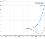
(a) $(1,3,3,2)$

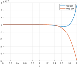
(b) $(5,6,3,2)$

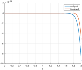
(c) $(6,8,18,11)$

Figure 4.1: Plots of integrand along the integration contour $\Gamma_{1}$ with $\ell=\ell^{\prime}=1$ and different $(n,n^{\prime},m,m^{\prime})$.

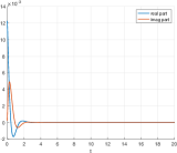
(a) $(1,3,3,2)$

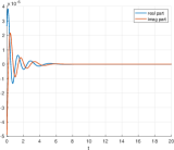
(b) $(5,6,3,2)$

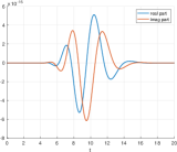
(c) $(6,8,18,11)$

Figure 4.2: Plots of integrand along the integration contour $\Gamma_{2}$ with $\ell=\ell^{\prime}=1$ and different $(n,n^{\prime},m,m^{\prime})$.

As an example, we plot the integrand in (4.33) along $\Gamma_{1}$ and $\Gamma_{2}$ (see, Fig. 4.1 and Fig. 4.2). The three layers case with $k_{0}=0.8,k_{1}=1.5,k_{2}=2.0,d=2.0,z=-0.3,z^{\prime}=-0.5$ and density given in (7.23) is used. We can see that the integrand has exponential decay along $\Gamma_{2}$ as $t$ goes to infinity.

Remark 4.2.

Similar to the first TE-FMM, the translation operators for center shift from source boxes to their parents and from target boxes to their children are exactly the same as in free space case which are given by (4.18) and (4.22).

The algorithm using symmetric derivatives for general component (3.17) is as following:

Algorithm 3 TEFMM-II for general component (3.17)

Generate an adaptive hierarchical tree structure and precompute tables.

Upward pass:

for $l=H\to 0$ do

     for all boxes $j$ on source tree level $l$  do

         if $j$ is a leaf node then

              form the free-space TE using Eq. (4.10).

         else

              form the free-space TE by merging children’s expansions using the free-space center shift translation operator (4.18).

         end if

     end for

end for

Downward pass:

for $l=1\to H$ do

     for all boxes $j$ on target tree level $l$  do

         shift the TE of $j$’s parent to $j$ itself using the free-space center shift translation operator (4.22).

         collect interaction list contribution using the source box to target box translation operator in Eq. (4.30) with precomputed tables of integrals (4.33).

     end for

end for

Evaluate Local Expansions:

for each leaf node (childless box) do

     evaluate the local expansion at each particle location using (4.11).

end for

Local Direct Interactions:

for $i=1\to N$  do

     compute Eq. (3.17) of target particle $i$ in the neighboring boxes using precomputed table of $u_{\ell\ell^{\prime}}^{\uparrow}(\bm{r},\bm{r}^{\prime})$.

end for

5 Numerical results

In this section, we present numerical results to demonstrate the performance of two versions of TE-FMMs for acoustic wave scattering in layered media. These algorithms are implemented based on an open-source FMM package DASHMM [37]. The numerical simulations are performed on a workstation with two Xeon E5-2699 v4 2.2 GHz processors (each has 22 cores) and 500GB RAM using the gcc compiler version 6.3. Two and three layers media are considered for the numerical tests. More specifically, interfaces are placed at $z_{0}=0$ and $z_{0}=0,z_{1}=-2$ for two and three layer cases, respectively. We first use an example with particles uniformly distributed inside a cubic domain for accuracy and efficiency test. Then, more general distributions of particles in irregular domains are tested.

Example 1 (Cubic domains): Set particles to be uniformly distributed in cubes of size $1$ centered at $(0.5,0.5,1.0)$, $(0.5,0.5,-1.0)$ and $(0.5,0.5,-3.0)$, respectively. Let $\widetilde{\Phi}_{\ell}(\bm{r}_{\ell i})$ be the approximated values of $\Phi_{\ell}(\bm{r}_{\ell i})$ calculated by TE-FEM. For accuracy test, we put $N=8000$ particles in each box and define $L^{2}$-error and maximum error as

$$Err_{2}^{\ell}:=\sqrt{\frac{\sum\limits_{i=1}^{N_{\ell}}|\Phi_{\ell}(\bm{r}_{\ell i})-\widetilde{\Phi}_{\ell}(\bm{r}_{\ell i})|^{2}}{\sum\limits_{i=1}^{N_{\ell}}|\Phi_{\ell}(\bm{r}_{\ell i})|^{2}}},\qquad Err_{max}^{\ell}:=\max\limits_{1\leq i\leq{N_{\ell}}}\frac{|\Phi_{\ell}(\bm{r}_{\ell i})-\widetilde{\Phi}_{\ell}(\bm{r}_{\ell i})|}{|\Phi_{\ell}(\bm{r}_{\ell i})|}.$$ (5.1)

Convergence rates against $p$ are depicted in Figs. 5.1 and 5.2. Comparisons between CPU time for the computation of free space components $\Phi_{\ell}^{free}$ and scattering components in two and three layers are presented in Tables 5.1-5.2 and Tables 5.3-5.4. We can see that the cost for the computation of scattering components is about forty times of that for the free space components.

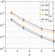
(a) two layers

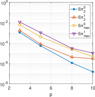
(b) three layers

Figure 5.1: Convergence of TEFMM-I against truncation number $p$.

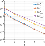
(a) two layers

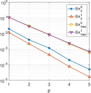
(b) three layers

Figure 5.2: Convergence of TEFMM-II against truncation number $p$.

cores	$N$	time for $\Phi_{0}^{free}$	time for $\Phi_{00}^{\uparrow}+\Phi_{01}^{\uparrow}$	time for $\Phi_{1}^{free}$	time for $\Phi_{10}^{\downarrow}+\Phi_{11}^{\downarrow}$
1	64000	4.11	120.11	4.00	135.57
	216000	25.65	902.09	25.73	1005.43
	512000	36.80	1120.73	36.58	1385.88
	1000000	61.84	1422.70	63.07	1539.35
22	64000	0.25	7.08	0.23	7.85
	216000	1.54	52.79	1.55	59.04
	512000	2.21	65.88	2.18	73.65
	1000000	3.75	81.39	3.65	90.25
44	64000	0.17	3.63	0.17	3.95
	216000	1.10	26.60	1.09	29.86
	512000	1.44	33.42	1.44	37.31
	1000000	1.92	41.34	1.88	45.84

Table 5.1: CPU time for two layers using TEFMM-I with $p=3$.

cores	$N$	time for $\Phi_{0}^{free}$	time for $\sum\limits_{\ell^{\prime}=0}^{2}\Phi_{0\ell^{\prime}}^{\uparrow}$	time for $\Phi_{1}^{free}$	time for $\sum\limits_{\ell^{\prime}=0}^{2}\Phi_{1\ell^{\prime}}^{\uparrow}$
1	64000	3.94	109.61	3.97	134.37
	216000	25.60	824.29	25.76	1016.34
	512000	36.74	1034.80	36.51	1266.90
	1000000	62.67	1286.97	60.39	1551.25
22	64000	0.25	6.47	0.24	7.90
	216000	1.55	48.26	1.55	59.32
	512000	2.21	60.36	2.19	73.81
	1000000	3.75	75.05	3.65	90.67
44	64000	0.16	3.34	0.17	3.99
	216000	1.09	24.38	1.09	30.06
	512000	1.60	30.73	1.62	37.75
	1000000	1.93	38.19	1.87	46.08

Table 5.2: CPU time for three layers using TEFMM-I with $p=3$.

cores	$N$	time for $\Phi_{0}^{free}$	time for $\Phi_{00}^{\uparrow}+\Phi_{01}^{\uparrow}$	time for $\Phi_{1}^{free}$	time for $\Phi_{10}^{\downarrow}+\Phi_{11}^{\downarrow}$
1	64000	7.65	120.27	7.37	117.20
	216000	60.76	610.60	59.30	663.51
	512000	60.80	1071.95	60.06	1049.38
	1000000	120.18	1153.79	118.06	1146.19
22	64000	0.38	9.48	0.38	9.64
	216000	3.41	54.53	3.43	55.94
	512000	3.47	74.21	3.43	74.84
	1000000	6.49	79.62	6.37	82.53
44	64000	0.23	8.35	0.21	8.72
	216000	1.74	47.62	1.76	47.09
	512000	1.75	66.88	1.73	65.65
	1000000	3.36	67.56	3.29	65.50

Table 5.3: CPU time for two layers using TEFMM-II with $p=3$.

cores	$N$	time for $\Phi_{0}^{free}$	time for $\sum\limits_{\ell^{\prime}=0}^{2}\Phi_{0\ell^{\prime}}^{\uparrow}$	time for $\Phi_{1}^{free}$	time for $\sum\limits_{\ell^{\prime}=0}^{2}\Phi_{1\ell^{\prime}}^{\uparrow}$
1	64000	6.66	97.98	6.58	99.07
	216000	60.42	651.24	61.14	657.92
	512000	64.91	912.75	63.15	903.19
	1000000	117.90	1101.38	116.92	1304.45
22	64000	0.38	9.64	0.38	9.69
	216000	3.41	54.79	3.42	56.29
	512000	3.47	75.98	3.41	75.91
	1000000	6.49	81.98	6.37	84.57
44	64000	0.22	8.06	0.22	8.52
	216000	1.77	47.69	1.80	46.63
	512000	1.74	66.45	1.74	65.43
	1000000	3.35	66.85	3.26	70.04

Table 5.4: CPU time for three layers using TEFMM-II with $p=3$.

Example 2 (Irregular domains): In practical applications, objects of irregular shape are often encountered. Here, we give examples with particles located in irregular domains which are obtained by shifting the domain given by

$$r=0.5-a+\frac{a}{8}(35\cos^{4}\theta-30\cos^{2}\theta+3),$$ (5.2)

with $a=0.1,0.15$ to new centers $(0,0,1)$ and $(0,0,-1)$, respectively (see Fig. 5.3 (left) for an illustration). For the three layer case test, we use particles in similar domains centered at $(0,0,1)$, $(0,0,-1)$ and $(0,0,-3)$ with $a=0.1,0.15,0.05$, respectively (see Fig. 5.3 (right)). All particles are generated by keeping the uniform distributed particles in a larger cubic within corresponding irregular domains. The CPU time for the computation of $\{\Phi_{\ell}(\bm{r}_{\ell i})\}_{i=0}^{N_{\ell}}$ and $\{\Phi_{\ell}^{free}(\bm{r}_{\ell i})\}_{i=0}^{N_{\ell}}$ are compared in Fig. 5.4 and Fig. 5.5. It shows that the new algorithms have an $O(N)$ complexity.

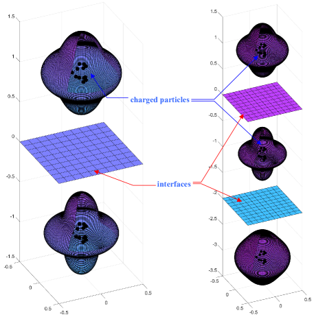
Figure 5.3: Configuration of two numerical examples.

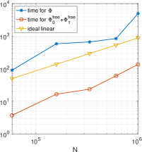
(a) two layers

(b) three layers

Figure 5.4: CPU time for TEFMM-I.

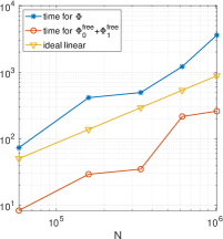
(a) two layers

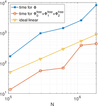
(b) three layers

Figure 5.5: CPU time for TEFMM-II.

6 Conclusion

In this paper, we have presented two Taylor-expansion based fast multipole method for the efficient calculation of the discretized integral operator for the Helmholtz equation in layered media. These methods use the Taylor expansion of layered media Green’s function for the low rank representation of far field for acoustic wave scattering governed by the Helmholtz equation. Comparing with the spherical harmonic multipole expansion in the traditional FMM, the Taylor expansion requires $O(p^{3})$ terms for the low rank representation of far field of layered Green’s function in contrast to $O(p^{2})$ for the spherical harmonic based multipole expansion FMM for the free space Green’s function. We addressed the main difficulty in developing the TE-FMM for the layered media - the computation of up to $p$-th order derivatives of the layered Green’s function, which are given in terms of oscillatory Sommerfeld integrals. We proposed two solutions to overcome this difficulty. For the first TE-FMM based on non-symmetric derivatives, an efficient algorithm was developed using discrete complex image, which has shown to be very accurate and efficient for the low frequency Helmholtz equation. Meanwhile, for the second TE-FMM based on symmetric derivatives, pre-calculated tables are used for the translation operators.

Both versions of the TE-FMM have comparable accuracy, and as our numerical examples show, both have an $O(N)$ time complexity similar to the FMM in the free space and they can provide fast solutions for integral equations of Helmholtz equations in layered media with low to middle frequencies. In comparison, the advantage of the first TE-FMM is the efficiency of computing the translation operator with the complex image approximations. However, the complex image approximation is sensitive to the parameters and we still need a rigorous mathematical theory for the approach in finding the discrete images. On the other hand, the second TE-FMM could be used for higher order TE expansions, however, there is a need to pre-compute large number of tables for the translation operators and it requires table storages.

For the future work, we will carry out error estimate of the TE-FMMs for the layered media, which require an analysis of the Sommerfeld integral representations of the derivatives and the complex image approximations.

7 Appendix A

7.1 Two layers with sources in the top layer

Let $L=1$ with source in the bottom layer at $\bm{r}^{\prime}=(x^{\prime},y^{\prime},z^{\prime})$, i.e., $z^{\prime}>0$. Then, the domain Green’s function has representation

$$\begin{cases}\widehat{u}_{0}(k_{x},k_{y},z)=A_{0}\cosh({\rm i}k_{0z}z)+B_{0}\sinh({\rm i}k_{0z}z)+\frac{{\rm i}e^{{\rm i}(k_{0z}|z-z^{\prime}|-k_{x}x^{\prime}-k_{y}y^{\prime})}}{2k_{0z}},&z>0,\\[7.0pt] \widehat{u}_{1}(k_{x},k_{y},z)=A_{1}\cosh({\rm i}k_{1z}z)+B_{1}\sinh({\rm i}k_{1z}z),&z<0,\end{cases}$$ (7.1)

or equivalently

$$\begin{cases}\widehat{u}_{0}(k_{x},k_{y},z)=b_{0}e^{{\rm i}k_{0z}z}+\frac{{\rm i}e^{{\rm i}(k_{0z}|z-z^{\prime}|-k_{x}x^{\prime}-k_{y}y^{\prime})}}{2k_{0z}},&z>0,\\[7.0pt] \widehat{u}_{1}(k_{x},k_{y},z)=a_{1}e^{-{\rm i}k_{1z}z},&z<0,\end{cases}$$ (7.2)

where

$$\begin{split}&b_{0}=\frac{A_{0}+B_{0}}{2},\quad a_{1}=\frac{A_{1}-B_{1}}{2}.\end{split}$$ (7.3)

Proceeding the recursion (2.3) gives coefficients

$$\begin{cases}\displaystyle A_{0}=B_{0}=\frac{(k_{0}k_{0z}-k_{1}k_{1z})e^{{\rm i}k_{0z}z^{\prime}}}{2(k_{0}k_{0z}+k_{1}k_{1z})}\frac{{\rm i}e^{-{\rm i}(k_{x}x^{\prime}+k_{y}y^{\prime})}}{k_{0z}},\\[10.0pt] \displaystyle A_{1}=-B_{1}=\frac{k_{0}k_{0z}e^{{\rm i}k_{0z}z^{\prime}}}{k_{0}k_{0z}+k_{1}k_{1z}}\frac{{\rm i}e^{-{\rm i}(k_{x}x^{\prime}+k_{y}y^{\prime})}}{k_{0z}},\end{cases}$$ (7.4)

or alternatively

$$\begin{cases}\displaystyle b_{0}=\frac{k_{0}k_{0z}-k_{1}k_{1z}}{2(k_{0}k_{0z}+k_{1}k_{1z})}\frac{{\rm i}e^{-{\rm i}(k_{x}x^{\prime}+k_{y}y^{\prime})}e^{{\rm i}k_{0z}z^{\prime}}}{k_{0z}},\\[10.0pt] \displaystyle a_{1}=\frac{k_{0}k_{1z}}{k_{0}k_{0z}+k_{1}k_{1z}}\frac{{\rm i}e^{-{\rm i}(k_{x}x^{\prime}+k_{y}y^{\prime})}e^{{\rm i}k_{0z}z^{\prime}}}{k_{1z}}.\end{cases}$$ (7.5)

Taking inverse Fourier transform on (7.2) with coefficients given by (7.5), we have

$$\sigma_{00}^{\uparrow\uparrow}(k_{\rho})=\frac{k_{0}k_{0z}-k_{1}k_{1z}}{k_{0}k_{0z}+k_{1}k_{1z}},\quad\sigma_{10}^{\downarrow\uparrow}(k_{\rho})=\frac{2k_{0}k_{1z}}{k_{0}k_{0z}+k_{1}k_{1z}}.$$ (7.6)

7.2 Two layers with sources in the bottom layer

Let $L=1$ with source in the bottom layer at $\bm{r}^{\prime}=(x^{\prime},y^{\prime},z^{\prime})$, i.e., $z^{\prime}<0$. The domain Green’s function has representation

$$\begin{cases}\widehat{u}_{0}(k_{x},k_{y},z)=A_{0}\cosh({\rm i}k_{0z}z)+B_{0}\sinh({\rm i}k_{0z}z),&z>0,\\[7.0pt] \widehat{u}_{1}(k_{x},k_{y},z)=A_{1}\cosh({\rm i}k_{1z}z)+B_{1}\sinh({\rm i}k_{1z}z)+\frac{{\rm i}e^{{\rm i}(k_{1z}|z-z^{\prime}|-k_{x}x^{\prime}-k_{y}y^{\prime})}}{2k_{1z}},&z<0,\end{cases}$$ (7.7)

or equivalently

$$\begin{cases}\widehat{u}_{0}(k_{x},k_{y},z)=b_{0}e^{{\rm i}k_{0z}z},&z>0,\\[7.0pt] \widehat{u}_{1}(k_{x},k_{y},z)=a_{1}e^{-{\rm i}k_{1z}z}+\frac{{\rm i}e^{{\rm i}(k_{1z}|z-z^{\prime}|-k_{x}x^{\prime}-k_{y}y^{\prime})}}{2k_{1z}},&z<0,\end{cases}$$ (7.8)

where

$$\begin{split}&b_{0}=\frac{A_{0}+B_{0}}{2},\quad a_{1}=\frac{A_{1}-B_{1}}{2}.\end{split}$$ (7.9)

Proceeding the recursion (2.3) gives coefficients

$$\begin{cases}\displaystyle A_{0}=B_{0}=\frac{e^{-{\rm i}k_{1z}z^{\prime}}k_{1}k_{1z}}{k_{0}k_{0z}+k_{1}k_{1z}}\frac{{\rm i}e^{-{\rm i}(k_{x}x^{\prime}+k_{y}y^{\prime})}}{k_{1z}},\\[10.0pt] \displaystyle A_{1}=-B_{1}=\frac{k_{1}k_{1z}-k_{0}k_{0z}}{2(k_{0}k_{0z}+k_{1}k_{1z})}\frac{{\rm i}e^{-{\rm i}(k_{x}x^{\prime}+k_{y}y^{\prime})}e^{-{\rm i}k_{1z}z^{\prime}}}{k_{1z}},\end{cases}$$ (7.10)

or alternatively

$$\begin{cases}\displaystyle b_{0}=\frac{k_{1}k_{0z}}{k_{0}k_{0z}+k_{1}k_{1z}}\frac{{\rm i}e^{-{\rm i}(k_{x}x^{\prime}+k_{y}y^{\prime})}e^{-{\rm i}k_{1z}z^{\prime}}}{k_{0z}},\\[10.0pt] \displaystyle a_{1}=\frac{k_{1}k_{1z}-k_{0}k_{0z}}{2(k_{0}k_{0z}+k_{1}k_{1z})}\frac{{\rm i}e^{-{\rm i}(k_{x}x^{\prime}+k_{y}y^{\prime})}e^{-{\rm i}k_{1z}z^{\prime}}}{k_{1z}}.\end{cases}$$ (7.11)

Taking inverse Fourier transform on (7.8) with coefficients given by (7.11), we have

$$\sigma_{01}^{\uparrow\downarrow}(k_{\rho})=\frac{2k_{1}k_{0z}}{k_{0}k_{0z}+k_{1}k_{1z}},\quad\sigma_{11}^{\downarrow\downarrow}(k_{\rho})=\frac{k_{1}k_{1z}-k_{0}k_{0z}}{k_{0}k_{0z}+k_{1}k_{1z}}.$$ (7.12)

7.3 Three layers with sources in the top layer

Let $L=2$ with interfaces at $z=0$ and $z=-d<0$. Assume that the source is in the first layer at $(x^{\prime},y^{\prime},z^{\prime})$, i.e., $z^{\prime}>0$. The domain Green’s function has representation

$$\begin{cases}\displaystyle\widehat{u}_{0}(k_{x},k_{y},z)=A_{0}\cosh({\rm i}k_{0z}z)+B_{0}\sinh({\rm i}k_{0z}z)+\frac{{\rm i}e^{{\rm i}(k_{0z}|z-z^{\prime}|-k_{x}x^{\prime}-k_{y}y^{\prime})}}{2k_{0z}},&0<z<z^{\prime},\\[7.0pt] \displaystyle\widehat{u}_{1}(k_{x},k_{y},z)=A_{1}\cosh({\rm i}k_{1z}(z+d))+B_{1}\sinh({\rm i}k_{1z}(z+d)),&-d<z<0,\\[7.0pt] \displaystyle\widehat{u}_{2}(k_{x},k_{y},z)=A_{2}\cosh({\rm i}k_{2z}z)+B_{2}\sinh({\rm i}k_{2z}z),&z<-d,\end{cases}$$ (7.13)

or equivalently

$$\begin{cases}\displaystyle\widehat{u}_{0}(k_{x},k_{y},z)=b_{0}e^{{\rm i}k_{0z}z}+\frac{{\rm i}e^{{\rm i}(k_{0z}|z-z^{\prime}|-k_{x}x^{\prime}-k_{y}y^{\prime})}}{2k_{0z}},&z>0,\\[7.0pt] \displaystyle\widehat{u}_{1}(k_{x},k_{y},z)=a_{1}e^{-{\rm i}k_{1z}(z+d)}+b_{1}e^{{\rm i}k_{1z}(z+d)},&-d<z<0,\\[7.0pt] \displaystyle\widehat{u}_{2}(k_{x},k_{y},z)=a_{2}e^{-{\rm i}k_{2z}z},&z<-d,\end{cases}$$ (7.14)

where

$$b_{0}=\frac{A_{0}+B_{0}}{2},\quad a_{1}=\frac{A_{1}-B_{1}}{2},\quad b_{1}=\frac{A_{1}+B_{1}}{2},\quad a_{2}=\frac{A_{2}-B_{2}}{2}.$$

Again proceeding the recursion (2.3) gives coefficients

$$\begin{cases}\displaystyle A_{0}=B_{0}=\frac{k_{0}k_{0z}\kappa_{11}+{\rm i}k_{1}k_{1z}\kappa_{12}}{2(k_{0}k_{0z}\kappa_{11}-{\rm i}k_{1}k_{1z}\kappa_{12})}\frac{{\rm i}e^{-{\rm i}(k_{x}x^{\prime}+k_{y}y^{\prime})}e^{{\rm i}k_{0z}z^{\prime}}}{k_{0z}},\\[7.0pt] \displaystyle A_{1}=\frac{k_{0}k_{1}k_{0z}k_{1z}}{k_{0}k_{0z}\kappa_{11}-{\rm i}k_{1}k_{1z}\kappa_{12}}\frac{{\rm i}e^{-{\rm i}(k_{x}x^{\prime}+k_{y}y^{\prime})}e^{ik_{0z}z^{\prime}}}{k_{0z}},\\[7.0pt] \displaystyle B_{1}=\frac{-k_{0}k_{2}k_{0z}k_{2z}}{k_{0}k_{0z}\kappa_{11}-{\rm i}k_{1}k_{1z}\kappa_{12}}\frac{{\rm i}e^{-{\rm i}(k_{x}x^{\prime}+k_{y}y^{\prime})}e^{ik_{0z}z^{\prime}}}{k_{0z}},\\[7.0pt] \displaystyle A_{2}=-B_{2}=\frac{k_{0}k_{1}k_{0z}k_{1z}e^{-{\rm i}dk_{2z}}}{k_{0}k_{0z}\kappa_{11}-{\rm i}k_{1}k_{1z}\kappa_{12}}\frac{{\rm i}e^{-{\rm i}(k_{x}x^{\prime}+k_{y}y^{\prime})}e^{{\rm i}k_{0z}z^{\prime}}}{k_{0z}},\end{cases}$$ (7.15)

and

$$\begin{cases}\displaystyle b_{0}=\frac{k_{0}k_{0z}\kappa_{11}+{\rm i}k_{1}k_{1z}\kappa_{12}}{2(k_{0}k_{0z}\kappa_{11}-{\rm i}k_{1}k_{1z}\kappa_{12})}\frac{{\rm i}e^{-{\rm i}(k_{x}x^{\prime}+k_{y}y^{\prime})}e^{{\rm i}k_{0z}z^{\prime}}}{k_{0z}},\\[7.0pt] \displaystyle a_{1}=\frac{k_{0}k_{1z}(k_{1}k_{1z}+k_{2}k_{2z})}{2(k_{0}k_{0z}\kappa_{11}-{\rm i}k_{1}k_{1z}\kappa_{12})}\frac{{\rm i}e^{-{\rm i}(k_{x}x^{\prime}+k_{y}y^{\prime})}e^{{\rm i}k_{0z}z^{\prime}}}{k_{1z}},\\[7.0pt] \displaystyle b_{1}=\frac{k_{0}k_{1z}(k_{1}k_{1z}-k_{2}k_{2z})}{2(k_{0}k_{0z}\kappa_{11}-{\rm i}k_{1}k_{1z}\kappa_{12})}\frac{{\rm i}e^{-{\rm i}(k_{x}x^{\prime}+k_{y}y^{\prime})}e^{{\rm i}k_{0z}z^{\prime}}}{k_{1z}},\\[7.0pt] \displaystyle a_{2}=\frac{k_{0}k_{1}k_{1z}k_{2z}e^{-{\rm i}dk_{2z}}}{k_{0}k_{0z}\kappa_{11}-{\rm i}k_{1}k_{1z}\kappa_{12}}\frac{{\rm i}e^{-{\rm i}(k_{x}x^{\prime}+k_{y}y^{\prime})}e^{{\rm i}k_{0z}z^{\prime}}}{k_{2z}},\end{cases}$$

where

$$\begin{split}&\kappa_{11}=\frac{k_{1}k_{1z}-k_{2}k_{2z}}{2}e^{{\rm i}2dk_{1z}}+\frac{k_{1}k_{1z}+k_{2}k_{2z}}{2},\\ &\kappa_{12}={\rm i}\Big{(}\frac{k_{2}k_{2z}-k_{1}k_{1z}}{2}e^{{\rm i}2dk_{1z}}+\frac{k_{1}k_{1z}+k_{2}k_{2z}}{2}\Big{)}.\end{split}$$ (7.16)

Substuting into (7.14) and applying inverse Fourier transform, we have

$$\begin{cases}\displaystyle\sigma_{00}^{\uparrow\uparrow}(k_{\rho})=\frac{k_{0}k_{0z}\kappa_{11}+{\rm i}k_{1}k_{1z}\kappa_{12}}{k_{0}k_{0z}\kappa_{11}-{\rm i}k_{1}k_{1z}\kappa_{12}},\\[8.0pt] \displaystyle\sigma_{10}^{\uparrow\uparrow}(k_{\rho})=\frac{k_{0}k_{1z}(k_{1}k_{1z}-k_{2}k_{2z})e^{{\rm i}dk_{1z}}}{k_{0}k_{0z}\kappa_{11}-{\rm i}k_{1}k_{1z}\kappa_{12}},\\[8.0pt] \displaystyle\sigma_{10}^{\downarrow\uparrow}(k_{\rho})=\frac{k_{0}k_{1z}(k_{1}k_{1z}+k_{2}k_{2z})e^{{\rm i}dk_{1z}}}{k_{0}k_{0z}\kappa_{11}-{\rm i}k_{1}k_{1z}\kappa_{12}},\\[8.0pt] \displaystyle\sigma_{20}^{\downarrow\uparrow}(k_{\rho})=\frac{2k_{0}k_{1}k_{1z}k_{2z}e^{{\rm i}dk_{1z}}}{k_{0}k_{0z}\kappa_{11}-{\rm i}k_{1}k_{1z}\kappa_{12}}.\end{cases}$$ (7.17)

7.4 Three layers with sources in the middle layer

Let $L=2$ with interfaces at $z=0$ and $z=-d<0$. Assume that the source is in the middle layer at $(x^{\prime},y^{\prime},z^{\prime})$, i.e., $-d<z^{\prime}<0$. The domain Green’s function has representation

$$\begin{cases}\displaystyle\widehat{u}_{0}=A_{0}\cosh({\rm i}k_{0z}z)+B_{0}\sinh({\rm i}k_{0z}z),&z>0,\\[7.0pt] \displaystyle\widehat{u}_{0}=A_{1}\cosh({\rm i}k_{1z}(z+d))+B_{1}\sinh({\rm i}k_{1z}(z+d))+\frac{{\rm i}e^{{\rm i}(k_{1z}|z-z^{\prime}|-k_{x}x^{\prime}-k_{y}y^{\prime})}}{2k_{1z}},&-d<z<z^{\prime},\\[7.0pt] \displaystyle\widehat{u}_{2}=A_{2}\cosh({\rm i}k_{2z}z)+B_{2}\sinh({\rm i}k_{2z}z),&z<-d,\end{cases}$$ (7.18)

or equivalently

$$\begin{cases}\displaystyle\widehat{u}_{0}=b_{0}e^{{\rm i}k_{0z}z},&z>0,\\[7.0pt] \displaystyle\widehat{u}_{1}=a_{1}e^{-{\rm i}k_{1z}(z+d)}+b_{1}e^{{\rm i}k_{1z}(z+d)}+\frac{{\rm i}e^{{\rm i}(k_{1z}|z-z^{\prime}|-k_{x}x^{\prime}-k_{y}y^{\prime})}}{2k_{1z}},&-d<z<0,\\[7.0pt] \displaystyle\widehat{u}_{2}=a_{2}e^{-{\rm i}k_{2z}z},&z<-d,\end{cases}$$ (7.19)

where

$$b_{0}=\frac{A_{0}+B_{0}}{2},\quad a_{1}=\frac{A_{1}-B_{1}}{2},\quad b_{1}=\frac{A_{1}+B_{1}}{2},\quad a_{2}=\frac{A_{2}-B_{2}}{2}.$$

Again proceeding the recursion (2.3) gives coefficients

$$\begin{cases}\displaystyle A_{0}=B_{0}=\frac{k_{1}k_{1z}\kappa_{23}}{k_{0}k_{0z}\kappa_{11}-{\rm i}k_{1}k_{1z}\kappa_{12}}\frac{{\rm i}e^{-{\rm i}(k_{x}x^{\prime}+k_{y}y^{\prime})}}{k_{1z}},\\[7.0pt] \displaystyle A_{1}=\frac{(e^{-{\rm i}k_{1z}z^{\prime}}k_{1}k_{1z}(k_{1}k_{1z}-k_{0}k_{0z})+e^{{\rm i}k_{1z}(d+z^{\prime})}\kappa_{21})e^{{\rm i}dk_{1z}}}{k_{0}k_{0z}\kappa_{11}-{\rm i}k_{1}k_{1z}\kappa_{12}}\frac{{\rm i}e^{-{\rm i}(k_{x}x^{\prime}+k_{y}y^{\prime})}}{k_{1z}},\\[7.0pt] \displaystyle B_{1}=\frac{(e^{-{\rm i}k_{1z}z^{\prime}}k_{2}k_{2z}(k_{0}k_{0z}-k_{1}k_{1z})+e^{{\rm i}k_{1z}(d+z^{\prime})}\kappa_{21}^{\prime})e^{{\rm i}dk_{1z}}}{k_{0}k_{0z}\kappa_{11}-{\rm i}k_{1}k_{1z}\kappa_{12}}\frac{{\rm i}e^{-{\rm i}(k_{x}x^{\prime}+k_{y}y^{\prime})}}{k_{1z}},\\[7.0pt] \displaystyle A_{2}=-B_{2}=\frac{k_{1}k_{1z}\kappa_{22}e^{{\rm i}d(k_{1z}-k_{2z})}}{k_{0}k_{0z}\kappa_{11}-{\rm i}k_{1}k_{1z}\kappa_{12}}\frac{{\rm i}e^{-{\rm i}(k_{x}x^{\prime}+k_{y}y^{\prime})}}{k_{1z}},\end{cases}$$ (7.20)

where $\kappa_{11},\kappa_{12}$ are defined in (7.16) and

$$\begin{split}\kappa_{21}&=(k_{1}k_{1z}-k_{2}k_{2z})\Big{(}\frac{k_{1}k_{1z}-k_{0}k_{0z}}{2}e^{{\rm i}dk_{1z}}+\frac{k_{0}k_{0z}+k_{1}k_{1z}}{2}e^{-{\rm i}dk_{1z}}\Big{)},\\ \kappa_{21}^{\prime}&=(k_{1}k_{1z}-k_{2}k_{2z})\Big{(}\frac{k_{0}k_{0z}-k_{1}k_{1z}}{2}e^{{\rm i}dk_{1z}}+\frac{k_{0}k_{0z}+k_{1}k_{1z}}{2}e^{-{\rm i}dk_{1z}}\Big{)},\\ \kappa_{22}&=\frac{k_{1}k_{1z}+k_{0}k_{0z}}{2}e^{{\rm i}k_{1z}z^{\prime}}+\frac{k_{1}k_{1z}-k_{0}k_{0z}}{2}e^{-{\rm i}k_{1z}z^{\prime}},\\ \kappa_{23}&=\frac{k_{1}k_{1z}-k_{2}k_{2z}}{2}e^{{\rm i}k_{1z}(2d+z^{\prime})}+\frac{k_{1}k_{1z}+k_{2}k_{2z}}{2}e^{-{\rm i}k_{1z}z^{\prime}}.\end{split}$$

Noting that

$$\kappa_{21}+\kappa_{22}=(k_{0}k_{0z}+k_{1}k_{1z})e^{{\rm i}k_{1z}z^{\prime}},\quad\kappa_{21}-\kappa_{22}=(k_{0}k_{0z}-k_{1}k_{1z})e^{-{\rm i}k_{1z}z^{\prime}},$$ (7.21)

we further have

$$\begin{cases}\displaystyle b_{0}=\frac{{\rm i}e^{-{\rm i}(k_{x}x^{\prime}+k_{y}y^{\prime})}}{k_{0z}}\frac{k_{1}k_{0z}\kappa_{23}}{k_{0}k_{0z}\kappa_{11}-{\rm i}k_{1}k_{1z}\kappa_{12}},\\[7.0pt] \displaystyle a_{1}=\frac{{\rm i}e^{-{\rm i}(k_{x}x^{\prime}+k_{y}y^{\prime})}}{2k_{1z}}\frac{(k_{1}k_{1z}-k_{0}k_{0z})\kappa_{23}e^{{\rm i}dk_{1z}}}{k_{0}k_{0z}\kappa_{11}-{\rm i}k_{1}k_{1z}\kappa_{12}},\\[7.0pt] \displaystyle b_{1}=\frac{{\rm i}e^{-{\rm i}(k_{x}x^{\prime}+k_{y}y^{\prime})}}{2k_{1z}}\frac{(k_{1}k_{1z}-k_{2}k_{2z})\kappa_{22}e^{{\rm i}dk_{1z}}}{k_{0}k_{0z}\kappa_{11}-{\rm i}k_{1}k_{1z}\kappa_{12}},\\[7.0pt] \displaystyle a_{2}=\frac{{\rm i}e^{-{\rm i}(k_{x}x^{\prime}+k_{y}y^{\prime})}}{k_{2z}}\frac{k_{1}k_{2z}\kappa_{22}e^{{\rm i}dk_{1z}}e^{-{\rm i}dk_{2z}}}{k_{0}k_{0z}\kappa_{11}-{\rm i}k_{1}k_{1z}\kappa_{12}}.\end{cases}$$ (7.22)

Substuting into (7.19) and applying inverse Fourier transform, we have

$$\begin{cases}\displaystyle\{\sigma_{01}^{\uparrow\uparrow}(k_{\rho}),\sigma_{01}^{\uparrow\downarrow}(k_{\rho})\}=\frac{k_{1}k_{0z}}{k_{0}k_{0z}\kappa_{11}-{\rm i}k_{1}k_{1z}\kappa_{12}}\big{\{}(k_{1}k_{1z}-k_{2}k_{2z})e^{{\rm i}dk_{1z}},k_{1}k_{1z}+k_{2}k_{2z}\},\\[8.0pt] \displaystyle\{\sigma_{11}^{\uparrow\uparrow}(k_{\rho}),\sigma_{11}^{\uparrow\downarrow}(k_{\rho})\}=\frac{k_{1}k_{1z}-k_{2}k_{2z}}{k_{0}k_{0z}\kappa_{11}-{\rm i}k_{1}k_{1z}\kappa_{12}}\Big{\{}\frac{k_{1}k_{1z}+k_{0}k_{0z}}{2},\frac{k_{1}k_{1z}-k_{0}k_{0z}}{2}e^{{\rm i}dk_{1z}}\Big{\}},\\[8.0pt] \displaystyle\{\sigma_{11}^{\downarrow\uparrow}(k_{\rho}),\sigma_{11}^{\downarrow\downarrow}(k_{\rho})\}=\frac{(k_{1}k_{1z}-k_{0}k_{0z})e^{{\rm i}dk_{1z}}}{k_{0}k_{0z}\kappa_{11}-{\rm i}k_{1}k_{1z}\kappa_{12}}\Big{\{}\frac{k_{1}k_{1z}-k_{2}k_{2z}}{2}e^{{\rm i}dk_{1z}},\frac{k_{1}k_{1z}+k_{2}k_{2z}}{2}\Big{\}},\\[8.0pt] \displaystyle\{\sigma_{21}^{\downarrow\uparrow}(k_{\rho}),\sigma_{21}^{\downarrow\downarrow}(k_{\rho})\}=\frac{k_{1}k_{2z}e^{-{\rm i}dk_{2z}}}{k_{0}k_{0z}\kappa_{11}-{\rm i}k_{1}k_{1z}\kappa_{12}}\Big{\{}k_{1}k_{1z}+k_{0}k_{0z},(k_{1}k_{1z}-k_{0}k_{0z})e^{{\rm i}dk_{1z}}\Big{\}}.\end{cases}$$ (7.23)

7.5 Three layers with sources in the bottom layer

Let $L=2$ with interfaces at $z=0$ and $z=-d<0$. Assume that the source is in the bottom layer at $(x^{\prime},y^{\prime},z^{\prime})$, i.e., $z^{\prime}<-d$. The domain Green’s function has representation

$$\begin{cases}\displaystyle\widehat{u}_{0}(k_{x},k_{y},z)=A_{0}\cosh({\rm i}k_{0z}z)+B_{0}\sinh({\rm i}k_{0z}z),&z>0,\\[7.0pt] \displaystyle\widehat{u}_{1}(k_{x},k_{y},z)=A_{1}\cosh({\rm i}k_{1z}(z+d))+B_{2}\sinh({\rm i}k_{1z}(z+d)),,&-d<z<0,\\[7.0pt] \displaystyle\widehat{u}_{2}(k_{x},k_{y},z)=A_{2}\cosh({\rm i}k_{2z}z)+B_{2}\sinh({\rm i}k_{2z}z),&z<-d,\end{cases}$$ (7.24)

or equivalently

$$\begin{cases}\displaystyle\widehat{u}_{0}(k_{x},k_{y},z)=b_{0}e^{{\rm i}k_{0z}z},&z>0,\\[7.0pt] \displaystyle\widehat{u}_{1}(k_{x},k_{y},z)=a_{1}e^{-{\rm i}k_{1z}(z+d)}+b_{1}e^{{\rm i}k_{1z}(z+d)},&-d<z<0,\\[7.0pt] \displaystyle\widehat{u}_{2}(k_{x},k_{y},z)=a_{2}e^{-{\rm i}k_{2z}z}+\frac{{\rm i}e^{{\rm i}(k_{2z}|z-z^{\prime}|-k_{x}x^{\prime}-k_{y}y^{\prime})}}{2k_{2z}},&z<-d,\end{cases}$$ (7.25)

where

$$b_{0}=\frac{A_{0}+B_{0}}{2},\quad a_{1}=\frac{A_{1}-B_{1}}{2},\quad b_{1}=\frac{A_{1}+B_{1}}{2},\quad a_{2}=\frac{A_{2}^{U}-B_{2}^{U}}{2}.$$

then the solution can be calculated via (2.7), i.e.,

$$\begin{cases}\displaystyle A_{0}=B_{0}=\frac{k_{1}k_{1z}k_{2}k_{2z}e^{{\rm i}dk_{1z}}}{k_{2}k_{2z}\kappa_{31}-{\rm i}k_{1}k_{1z}\kappa_{32}}\frac{{\rm i}e^{-{\rm i}(k_{x}x^{\prime}+k_{y}y^{\prime})}e^{-{\rm i}k_{2z}(d+z^{\prime})}}{k_{2z}},\\[7.0pt] \displaystyle A_{1}=\frac{k_{2}k_{2z}\kappa_{31}e^{-{\rm i}k_{2z}(d+z^{\prime})}}{k_{2}k_{2z}\kappa_{31}-{\rm i}k_{1}k_{1z}\kappa_{32}}\frac{{\rm i}e^{-{\rm i}(k_{x}x^{\prime}+k_{y}y^{\prime})}}{k_{2z}},\\[7.0pt] \displaystyle B_{1}=\frac{-{\rm i}k_{2}k_{2z}\kappa_{32}e^{-{\rm i}k_{2z}(d+z^{\prime})}}{k_{2}k_{2z}\kappa_{31}-{\rm i}k_{1}k_{1z}\kappa_{32}}\frac{{\rm i}e^{-{\rm i}(k_{x}x^{\prime}+k_{y}y^{\prime})}}{k_{2z}},\\[7.0pt] \displaystyle A_{2}=-B_{2}=\frac{k_{2}k_{2z}\kappa_{31}+{\rm i}k_{1}k_{1z}\kappa_{32}}{2(k_{2}k_{2z}\kappa_{31}-{\rm i}k_{1}k_{1z}\kappa_{32})}\frac{{\rm i}e^{-{\rm i}(k_{x}x^{\prime}+k_{y}y^{\prime})}e^{-{\rm i}k_{2z}(d+z)}}{k_{2z}},\end{cases}$$ (7.26)

where

$$\begin{split}&\kappa_{31}=\frac{k_{1}k_{1z}-k_{0}k_{0z}}{2}e^{{\rm i}2dk_{1z}}+\frac{k_{1}k_{1z}+k_{0}k_{0z}}{2},\\ &\kappa_{32}={\rm i}\Big{(}\frac{k_{0}k_{0z}-k_{1}k_{1z}}{2}e^{{\rm i}2dk_{1z}}+\frac{k_{0}k_{0z}+k_{1}k_{1z}}{2}\Big{)}.\end{split}$$ (7.27)

Then

$$\begin{cases}\displaystyle b_{0}=\frac{k_{1}k_{1z}k_{2}k_{2z}e^{{\rm i}dk_{1z}}}{k_{2}k_{2z}\kappa_{31}+{\rm i}k_{1}k_{1z}\kappa_{32}}\frac{{\rm i}e^{-{\rm i}(k_{x}x^{\prime}+k_{y}y^{\prime})}e^{-{\rm i}k_{2z}(d+z^{\prime})}}{k_{2z}},\\[7.0pt] \displaystyle a_{1}=\frac{{\rm i}e^{-{\rm i}(k_{x}x^{\prime}+k_{y}y^{\prime})}}{k_{2z}}\frac{k_{2}k_{2z}(k_{1}k_{1z}-k_{0}k_{0z})e^{{\rm i}2dk_{1z}}e^{-{\rm i}k_{2z}(d+z^{\prime})}}{2(k_{2}k_{2z}\kappa_{31}+{\rm i}k_{1}k_{1z}\kappa_{32})},\\[7.0pt] \displaystyle b_{1}=\frac{{\rm i}e^{-{\rm i}(k_{x}x^{\prime}+k_{y}y^{\prime})}}{k_{2z}}\frac{k_{2}k_{2z}(k_{1}k_{1z}+k_{0}k_{0z})e^{-{\rm i}k_{2z}(d+z^{\prime})}}{2(k_{2}k_{2z}\kappa_{31}+{\rm i}k_{1}k_{1z}\kappa_{32})},\\[7.0pt] \displaystyle a_{2}=\frac{k_{2}k_{2z}\kappa_{31}+{\rm i}k_{1}k_{1z}\kappa_{32}}{2(k_{2}k_{2z}\kappa_{31}-{\rm i}k_{1}k_{1z}\kappa_{32})}\frac{{\rm i}e^{-{\rm i}(k_{x}x^{\prime}+k_{y}y^{\prime})}e^{-{\rm i}dk_{2z}}}{k_{2z}}.\end{cases}$$ (7.28)

Substuting into (7.25) and applying inverse Fourier transform, we have

$$\begin{cases}\displaystyle\sigma_{02}^{\uparrow\downarrow}(k_{\rho})=\frac{2k_{1}k_{1z}k_{2}k_{0z}e^{{\rm i}dk_{1z}}}{k_{2}k_{2z}\kappa_{31}-{\rm i}k_{1}k_{1z}\kappa_{32}},\\[8.0pt] \displaystyle\sigma_{12}^{\uparrow\downarrow}(k_{\rho})=\frac{k_{2}k_{1z}(k_{1}k_{1z}+k_{0}k_{0z})}{k_{2}k_{2z}\kappa_{31}-{\rm i}k_{1}k_{1z}\kappa_{32}},\\[8.0pt] \displaystyle\sigma_{12}^{\downarrow\downarrow}(k_{\rho})=\frac{k_{2}k_{1z}(k_{1}k_{1z}-k_{0}k_{0z})e^{{\rm i}2dk_{1z}}}{k_{2}k_{2z}\kappa_{31}-{\rm i}k_{1}k_{1z}\kappa_{32}},\\[8.0pt] \displaystyle\sigma_{22}^{\downarrow\downarrow}(k_{\rho})=\frac{k_{2}k_{2z}\kappa_{31}+{\rm i}k_{1}k_{1z}\kappa_{32}}{k_{2}k_{2z}\kappa_{31}-{\rm i}k_{1}k_{1z}\kappa_{32}}.\end{cases}$$ (7.29)

It is worthy to point out that

$$k_{2}k_{2z}\kappa_{31}-{\rm i}k_{1}k_{1z}\kappa_{32}=k_{0}k_{0z}\kappa_{11}-{\rm i}k_{1}k_{1z}\kappa_{12}.$$

References

- [1] K. A. Michalski, D. L. Zheng, Electromagnetic scattering and radiation by surfaces of arbitrary shape in layered media. I. theory, IEEE Trans. Antennas Propag. 38 (3) (1990) 335–344.
- [2] X. M. Millard, Q. H. Liu, A fast volume integral equation solver for electromagnetic scattering from large inhomogeneous objects in planarly layered media, IEEE Trans. Antennas Propag. 51 (9) (2003) 2393–2401.
- [3] D. Chen, M. H. Cho, W. Cai, Accurate and efficient Nystrm volume integral equation method for electromagnetic scattering of 3-D metamaterials in layered media, SIAM J. Sci. Comput. 40 (1) (2018) B259–B282.
- [4] J. Lai, M. Kobayashi, L. Greengard, A fast solver for multi-particle scattering in a layered medium, Opt. Express 22 (17) (2014) 20481–20499.
- [5] M. H. Cho, W. Cai, A parallel fast algorithm for computing the helmholtz integral operator in 3-d layered media, Journal of Computational Physics 231 (2012) 5910-5925.
- [6] M. H. Cho, Spectrally-accurate numerical method for acoustic scattering from doubly-periodic 3d multilayered media, arXiv preprint arXiv:1806.03813.
- [7] M. H. Cho, A. H. Barnett, Robust fast direct integral equation solver for quasi-periodic scattering problems with a large number of layers, Opt. express 23 (2) (2015) 1775–1799.
- [8] J. Lai, M. Kobayashi, A. Barnett, A fast and robust solver for the scattering from a layered periodic structure containing multi-particle inclusions, J. Comput. Phys. 298 (2015) 194–208.
- [9] L. Greengard, V. Rokhlin, A fast algorithm for particle simulations, J. Comput. phys. 73 (2) (1987) 325–348.
- [10] L. Greengard, V. Rokhlin, A new version of the fast multipole method for the laplace equation in three dimensions, Acta Numer. 6 (1997) 229–269.
- [11] Y. L. Chow, J. J. Yang, D. G. Fang, G. E. Howard, A closed-form spatial Green’s function for the thick microstrip substrate, IEEE Trans. Microwave Theory Tech. 39 (3) (1991) 588–592.
- [12] M. I. Aksun, A robust approach for the derivation of closed-form Green’s functions, IEEE Trans. Microw. Theory Tech. 44 (5) (1996) 651–658.
- [13] A. Alparslan, M. I. Aksun, K. A. Michalski, Closed-form Green’s functions in planar layered media for all ranges and materials, IEEE Trans. Microw. Theory Tech. 58 (3) (2010) 602–613.
- [14] V. Jandhyala, E. Michielssen, R. Mittra, Multipole-accelerated capacitance computation for 3-D structures in a stratified dielectric medium using a closed-form Green’s function, Int. J. Microwave Millimeter-Wave Computer-Aided Eng. 5 (2) (1995) 68–78.
- [15] L. Gurel, M. I. Aksun, Electromagnetic scattering solution of conducting strips in layered media using the fast multipole method, IEEE Microwave Guided Wave Lett. 6 (8) (1996) 277.
- [16] N. Geng, A. Sullivan, L. Carin, Fast multipole method for scattering from an arbitrary PEC target above or buried in a lossy half space, IEEE Trans. Antennas Propag. 49 (5) (2001) 740–748.
- [17] J. Tausch, The variable order fast multipole method for boundary integral equations of the second kind, Computing 72 (3-4) (2004) 267–291.
- [18] L. X. Ying, G. Biros, D. Zorin, A kernel-independent adaptive fast multipole algorithm in two and three dimensions, J. of Comput. Phys. 196 (2) (2004) 591–626.
- [19] W. Fong, E. Darve, The black-box fast multipole method, J. Comput. Phys. 228 (23) (2009) 8712–8725.
- [20] E. Darve, P. Havé, Efficient fast multipole method for low-frequency scattering, J. Comput. Phys. 197 (1) (2004) 341–363.
- [21] M. H. Cho, W. Cai, A parallel fast algorithm for computing the Helmholtz integral operator in 3-D layered media, J. Comput. Phys. 231 (17) (2012) 5910–5925.
- [22] P. J. Li, H. Johnston, R. Krasny, A Cartesian treecode for screened Coulomb interactions, J. Computat. Phys. 228 (10) (2009) 3858–3868.
- [23] J. Tausch, The fast multipole method for arbitrary Green’s functions, Contemporary Mathematics 329 (2003) 307–314.
- [24] W. Cai, Computational Methods for Electromagnetic Phenomena: electrostatics in solvation, scattering, and electron transport, Cambridge University Press, New York, NY, 2013.
- [25] W. Cai, T. J. Yu, Fast calculations of dyadic Green’s functions for electromagnetic scattering in a multilayered medium, J. Comput. Phys. 165 (1) (2000) 1–21.
- [26] V. I. Okhmatovski, A. C. Cangellaris, Evaluation of layered media Green’s functions via rational function fitting, IEEE microw. Wireless Comp. Lett. 14 (1) (2004) 22–24.
- [27] M. Paulus, P. Gay-Balmaz, O. J. F. Martin, Accurate and efficient computation of the Green’s tensor for stratified media, Physical Review E 62 (4) (2000) 5797.
- [28] D. G. Fang, J. J. Yang, G. Y. Delisle, Discrete image theory for horizontal electric dipoles in a multilayered medium, in: IEE Proc. H. Microw. Antennas and Propag., Vol. 135, IET, 1988, pp. 297–303.
- [29] M. Ochmann, The complex equivalent source method for sound propagation over an impedance plane, J. Acoust. Soc. Amer. 116 (6) (2004) 3304–3311.
- [30] I.-S. Koh, J.-G. Yook, Exact closed-form expression of a sommerfeld integral for the impedance plane problem, IEEE Trans. Antennas Propag. 54 (9) (2006) 2568–2576.
- [31] Y. L. Li, M. J. White, Near-field computation for sound propagation above ground using complex image theory, J. Acoust. Soc. Amer. 99 (2) (1996) 755–760.
- [32] F. Ling, J. M. Jin, Discrete complex image method for Green’s functions of general multilayer media, IEEE Microw. Guided Wave Lett. 10 (10) (2000) 400–402.
- [33] M. oneil, L. Greengard, A. Pataki, On the efficient representation of the half-space impedance Green’s function for the helmholtz equation, Wave Motion 51 (1) (2014) 1–13.
- [34] J. Lai, L. Greengard, M. O’Neil, A new hybrid integral representation for frequency domain scattering in layered media, Appl. Comput. Harmon. A. 45 (2) (2018) 359–378.
- [35] Y. B. Hua, T. K. Sarkar, Generalized pencil-of-function method for extracting poles of an EM system from its transient response, IEEE Trans. Antennas Propag. 37 (2) (1989) 229–234.
- [36] P. A. Martin, Multiple scattering: interaction of time-harmonic waves with N obstacles, no. 107, Cambridge University Press, 2006.
- [37] J. DeBuhr, B. Zhang, A. Tsueda, V. Tilstra-Smith, T. Sterling, Dashmm: Dynamic adaptive system for hierarchical multipole methods, Commun. Comput. Phys. 20 (4) (2016) 1106–1126.
- [38] B. Hu, W. C. Chew, Fast inhomogeneous plane wave algorithm for electromagnetic solutions in layered medium structures: two-dimensional case, Radio Sci. 35 (1) (2000) 31–43.
- [39] O. P. Bruno, M. Lyon, C. Pérez-Arancibia, C. Turc, Windowed green function method for layered-media scattering, SIAM Journal on Applied Mathematics 76 (5) (2016) 1871–1898.