The Impact of Spatial Correlation in Fluctuations of the Refractive Index on Rogue Wave Generation Probability

Abstract

The presence of refractive index fluctuations in an optical medium can result in the generation of optical rogue waves. Using numerical simulations and statistical analysis, we have shown that the probability of optical rogue waves increases in the presence of spatial correlations in the fluctuations of the refractive index. We have analyzed the impact of the magnitude and the spatial correlation length of these fluctuations on the probability of optical rogue wave generation.

I Introduction

Oceanic freak or rogue waves (RW) are large, rare, and unpredictable waves that appear in relatively calm waters, and are claimed to result in maritime disasters involving ship disappearances muller2005rogue . The science of RWs in optics was initiated by observing extraordinarily high field amplitude peaks at certain wavelengths in the chaotic spectrum from the supercontinuum solli2007optical . It is now understood that RWs can appear in different circumstances in both linear and nonlinear systems arecchi2011granularity ; akhmediev2010editorial ; Leonetti ; Safari . In recent years, numerous theoretical and experimental results have been reported on the generation and study of RWs in different optical platforms. Examples in nonlinear systems include supercontinuum generation in optical fibers solli2007optical ; lafargue2009direct ; solli2010seeded ; buccoliero2011midinfrared , nonlinear waves in optical cavities montina2009non ; residori2012rogue , and Raman fiber amplifiers finot2010selection ; hammani2012experimental . There have been only a few reports on studies of RWs in linear systems akhmediev2010editorial ; hohmann2010freak ; ying2011linear ; mattheakis2016extreme ; peysokhan2017optical . In particular, Ref. hohmann2010freak conducted a microwave transport experiment in a quasi-two-dimensional resonator with randomly distributed conical scatterers and found hot spots corresponding to RWs.

In this Letter, we expand on the results of Ref. hohmann2010freak and study the impact of the spatial correlation in the fluctuations of the material dielectric constant on the probability of RW generation. Our analysis targets the optical domain and the results are notable because in practice refractive index fluctuations always occur with a finite correlation length. In the examples that we explore in this Letter, we show that with increasing the correlation length, the probability of RW generation increases. We apply our analysis to examine whether the increased likelihood of hot spots (RWs) may be linked to premature material failure when exposed to high-intensity laser radiation rudolph2013laser . Our analysis is performed in the linear domain, similar to Ref. hohmann2010freak . We study the effect of the correlation length ($\mu$) and the dielectric constant fluctuation contrast (DCFC, $\Delta\epsilon$), which is defined as the difference between the maximum and the minimum of the dielectric constant, on the probability of occurrence of optical RWs. We show that both the correlation length and DCFC have significant impacts on the probability of RW generation.

II Simulations

Simulations are performed with the finite-difference time-domain (FDTD) method fdtd using Meep, which is an open-source software package for electromagnetics simulation meep . Meep simulates fully vectorial Maxwell’s equations:

$$\frac{\partial\mathbf{B}}{\partial t} =-\nabla\times\mathbf{E}-\mathbf{J}_{B}-\sigma_{B}\mathbf{B}, \mathbf{B}=\mu\mathbf{H},$$ (1)

$$\frac{\partial\mathbf{D}}{\partial t} =\nabla\times\mathbf{H}-\mathbf{J}-\sigma_{D}\mathbf{D}, \mathbf{D}=\varepsilon\mathbf{E},$$ (2)

where $\mathbf{E}$ is the electric field, $\mathbf{D}$ is displacement field, $\mathbf{H}$ is the magnetic field, and $\mathbf{B}$ is the magnetic flux density. $\varepsilon$ is the dielectric constant, $\mu$ is the magnetic permeability, $\mathbf{J}$ ($\mathbf{J}_{B}$) is the current density of electric (magnetic) charge, and $\sigma_{B}$ ($\sigma_{D}$) terms correspond to (frequency-independent) magnetic (electric) conductivities.

The occurrence of RWs is due to random fluctuations in the material; therefore, it must be studied using a statistical approach. For each dielectric medium identified with a particular value of DCFC and correlation length, we create an ensemble of “statistically equivalent” dielectric media mafi2015transverse . Each ensemble contains a sufficiently large number of elements required for obtaining proper statistics to estimate the probability of RW generation. The dielectric medium is assumed to have no absorption and is invariant in the y-direction, and light is incident along the z-direction. Both the width of the medium in the transverse x-direction and its length in the longitudinal z-direction are each chosen to be $100\lambda$. The incident light is a monochromatic plane-wave of wavelength $\lambda$, and the polarization of the light is perpendicular to the x-z plane. Perfectly matched layers of thickness $\lambda$ are placed all around the medium. The numerical cell size is set at $\lambda/15$, which is sufficiently small compared with the wavelength of light to ensure the accuracy of the computation. The background dielectric constant of the medium is assumed to be $\epsilon=2$. The propagation of the wave is computed until the steady state is established. Depending on the value of DCFC and correlation length, 2,000 to 5,000 simulations are performed in each case. Simulations are performed on 20 nodes of a supercomputer, where each node has 8 CPUs.

To construct the medium with a randomly fluctuating dielectric constant with a specific correlation length, we employ the following procedure: we first create a random vector $X$ representing the dielectric constant at each point on the 2D computational grid in the x-z plane. The dielectric constant on the computational grid is sampled at $N\,=\,$100 points in each spatial coordinate and is represented by indices $i,j=1,\cdots,N$. An element of $X$ is represented by $X_{\alpha}$, where $\alpha(i,j)=i+N\times j$; therefore, $X$ has $100^{2}=10,000$ elements. $X_{\alpha}$ consists of uncorrelated random variables, which are chosen uniformly in the range $[-\Delta\epsilon,\Delta\epsilon]$; therefore, $E(X_{\alpha})\,=0$ and $E(X_{\alpha},X_{\beta})\,=\,\Delta\epsilon^{2}/3$, where $\alpha,\beta\,=,1,\cdots\,N^{2}$. In matrix language, we have:

$$E(X)\,=0,\quad E(X,X^{T})\,=\,(\Delta\epsilon^{2}/3)\,{\mathbf{1}},$$ (3)

where $E$ represents the expectation value. To transform $X$ to a correlated random vector, we start with the desired covariance matrix $Q$ identified by the correlation length $\mu$. The elements of $Q$ are constructed according to:

$$Q_{\alpha,\beta}\,=\,\exp(-\tilde{d}(\alpha,\beta)/\mu^{2}),$$ (4)

where $\tilde{d}(\alpha,\beta)$ is the square of the physical distance between points $\alpha$ and $\beta$ on the computational grid. Therefore, the correlation between two points decreases exponentially as a function of their separation. We then use Cholesky decomposition to decompose the real symmetric positive-definite matrix $Q$ into a unique product of a lower triangular matrix $L$ with its transpose $L^{T}$:

$$Q=LL^{T}.$$ (5)

We then define another vector $Z=LX$ with the following property:

$$E(Z)\,=0,\quad E(Z,Z^{T})\,=\,(\Delta\epsilon^{2}/3)\,Q,$$ (6)

which represents the desired correlated random vector.

To simulate the propagation of light and RW generation in each element of an ensemble for a given value of $\Delta\epsilon$ and $\mu$, we generate a $Z$ vector, representing the fluctuations of the dielectric constant in that element. Although the variance of the elements of $Z$ are bounded by $\Delta\epsilon^{2}/3$, the size of the elements of $Z$ become occasionally larger than $\Delta\epsilon$, resulting in unacceptably large dielectric constant fluctuations. In such cases, we remove this element from the ensemble and generated another $Z$, ensuring that the size of each element remains smaller than or equal to $\Delta\epsilon$. By following this procedure, the correlation is persevered and the maximum values of fluctuation in the dielectric constant is guaranteed to remain below $\Delta\epsilon$ for a more realistic representation of a dielectric. Because of this selective elimination, the statistics will deviate slightly from the continuous uniform distribution, which is inconsequential in the general observations we present in this Letter.

III Results

In Fig. 1, the refractive index and light intensity profiles are shown for three different dielectric media with different values of the correlation length for refractive index fluctuations. From the top row to the bottom row, the correlation lengths are $0.2\lambda$, $1.3\lambda$, and $2.8\lambda$, respectively; $\Delta\epsilon=0.4$ is assumed in all three cases. The left column in Fig. 1 shows the refractive index fluctuations and the effect of the increased correlation length from top to bottom row is visible. The right column shows the intensity of the propagated light: in each case, the incident light is a plane-wave with the wavelength $\lambda$, which propagates along the z-direction (from left to right). The branching flow of light clearly appears in this linear regime, and several high-intensity spots are observed in each case. As the correlation length is increased, the number of branches decrease, but the peaks appear to become more prominent and intense. Therefore, it is desirable to investigate the impact of an increase in the correlation length of the refractive index fluctuation on the occurrence of the RWs quantitatively.

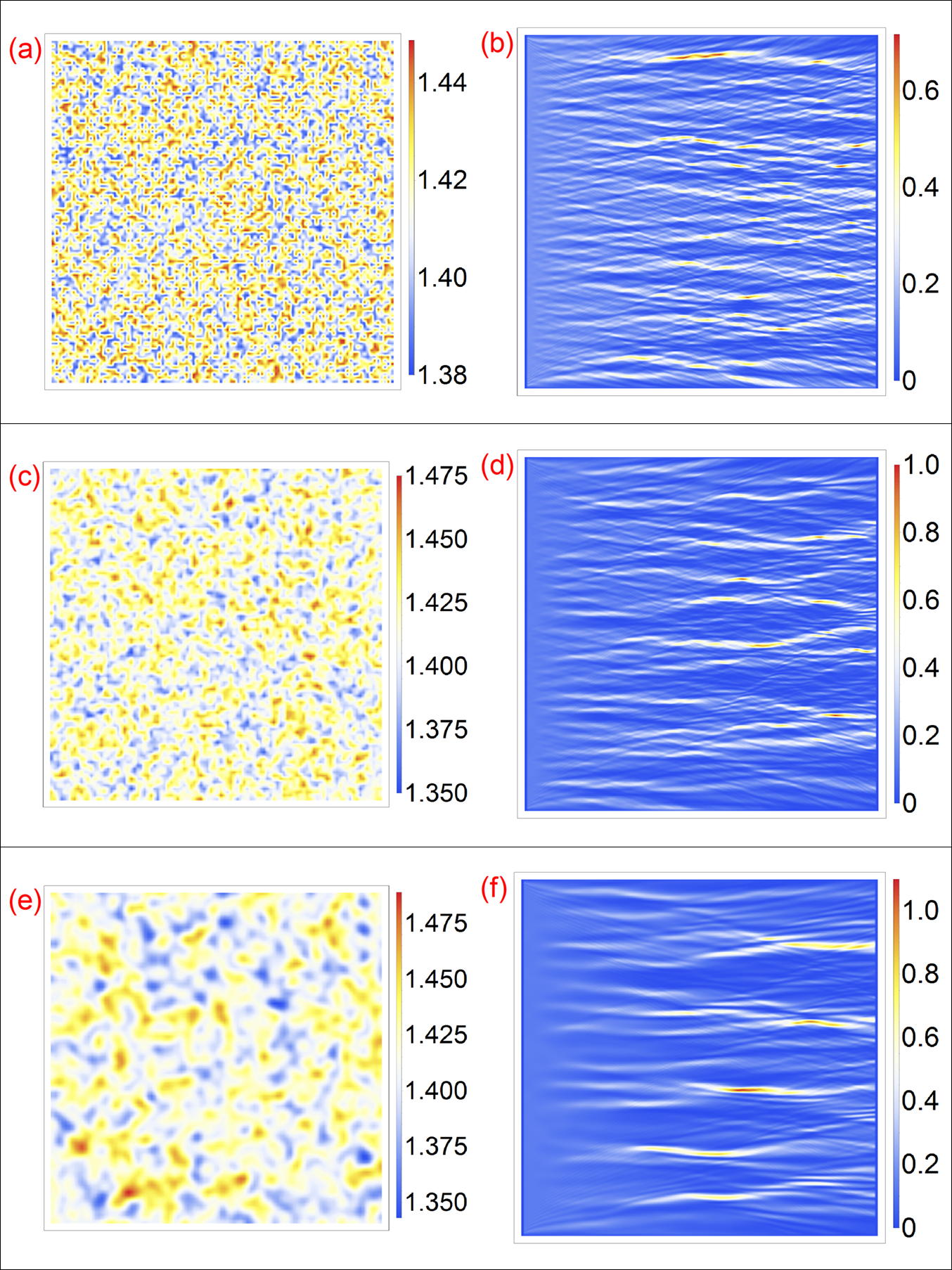
Figure 1: (a), (c), and (e) show the fluctuations in the refractive index profiles with the correlation lengths of $0.2\lambda$, $1.3\lambda$, and $2.8\lambda$, respectively, where $\Delta\epsilon=0.4$ is assumed in all three cases. (b), (d), and (f) show the light intensities related to (a), (c), and (e), respectively. The incident plane-wave propagates along the z-direction, from left to right.

To quantify the occurrence rate of the RWs, we first need to identify them. In Fig. 2, we show an example of the propagation of light through a randomly correlated dielectric medium, defined by $\Delta\epsilon=0.4$ and $\mu=2.8\lambda$. Figure 2(b) is a three-dimensional display of intensity, zoomed-in over the black square in Fig. 2(a), in which the optical RW is seen. To find the occurrence of an RW event, after steady-state of the propagated wave is established, the intensity of the optical field is extracted in the matrix format sampled at each position. Then a two-dimensional local intensity peak-detection procedure is performed over the intensity matrix, where each intensity pixel is compared to its eight neighbors, from which a peak intensity probability distribution (PIPD) is calculated. The PIPD, $P(I)$, is defined such that $P(I)\,dI$ is proportional to the number of local peaks in the intensity range of $I$ and $I+dI$.

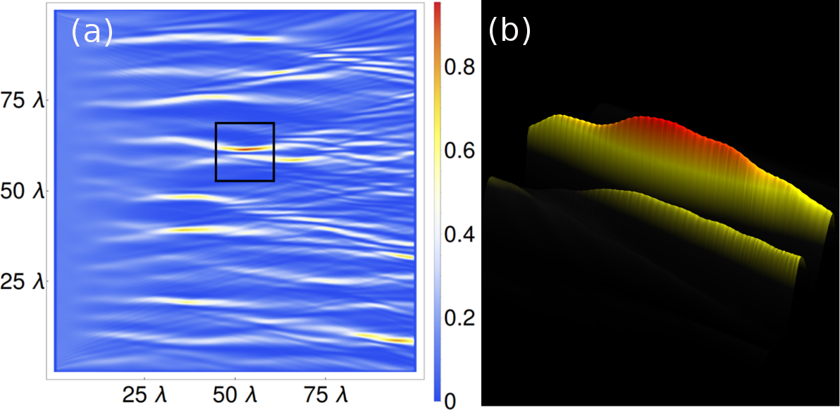
Figure 2: (a) The propagation of light through a random dielectric medium with $\mu=2.8\lambda$ and $\Delta\epsilon=0.4$ is shown. The incident light is a plane-wave with the wavelength $\lambda$. The light is propagated along the z-direction (from left to right). (b) A 3D display of the intensity corresponding to the black square region in subfigure (a) displays the profile of an optical RW.

To identify an intensity peak as a RW after PIPD is determined, one can use one of the following two commonly used methods: Method 1 is based on the Longuet-Higgins random seas model Longuet-Higgins , where the central limit theorem is applied to the random superposition of a large number of optical waves with different propagating directions, resulting in a Rayleigh probability distribution for the intensity peaks of the form $P(I)=e^{-I}$; and in Method 2 RWs are identified using the RW-intensity-threshold in PIPD. The RW-intensity-threshold ($I_{\rm RW}$) is given by $I_{\rm RW}=2I_{S}$, where $I_{S}$ is the mean of the upper third of peaks in the PIPD and all peak events with higher intensity than $I_{\rm RW}$ are identified as RWs dudley2014instabilities . In Fig. 3, we employ Method 2 to the configuration discussed in Fig. 2: the calculated PIPD is shown, where the peak events that satisfy $I_{\rm peak}>I_{\rm RW}$ are highlighted by a darker background color.

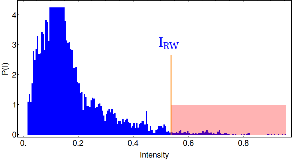
Figure 3: The simulations presented in this figure correspond to $\mu=2.8\lambda$ and $\Delta\epsilon=0.4$. The probability distribution of the peak intensities is plotted versus the intensity values of the peaks. The vertical orange line marked with $I_{RW}$ indicates the threshold of the optical RWs based on Method 2, above which the events are identified as RWs.

In this Letter, we use Method 2, which is also commonly used in the theory of scattering from random potentials. To evaluate the impact of the correlation length on the occurrence probability of RWs, we propagated an optical plane wave through a randomly correlated material with the same geometry and the dielectric contrast of $\Delta\epsilon=0.08$. The number of RWs is counted based on the statistical approach of Method 2. This process is repeated for 2000 different media (random realizations of the ensemble) for each value of the correlation length. Finally, the average and standard deviation of the number of RWs are calculated and the result is shown in Fig. 4. The average number of RWs increases by nearly two orders of magnitude when the correlation length increases from $0.2\lambda$ to $2.8\lambda$–this implies that the effect of correlation length is substantial on the probability of RW generation. This observation is the main finding in this Letter and the simulations are generic enough to suggest that this behavior is universal for at least a broad range of correlation lengths.

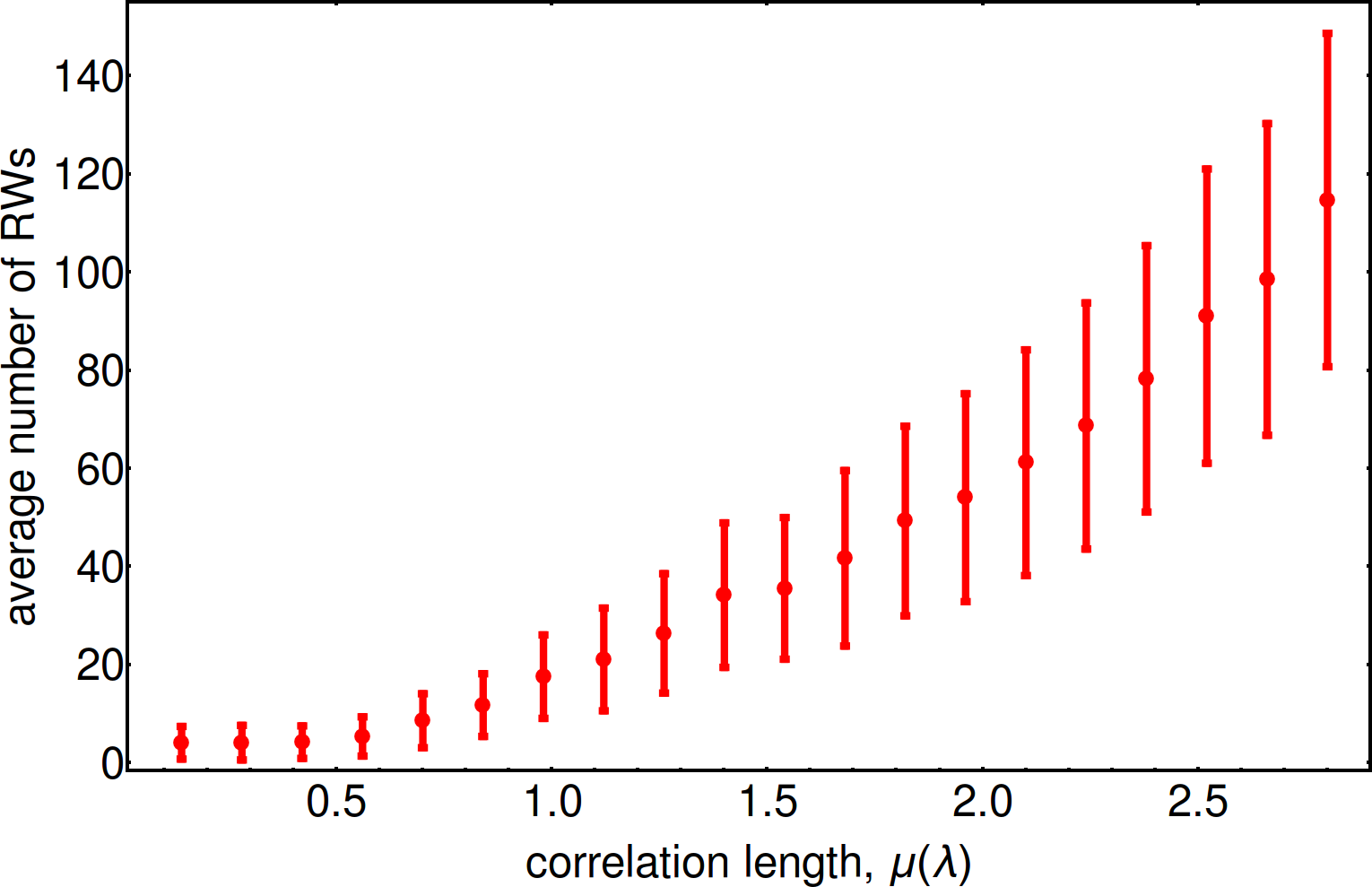
Figure 4: The number of RWs versus the correlation length: the dots are the average number of RWs for a specific correlation length and the error bars are the standard deviation of the total number of RWs for each correlation length.

Another parameter that plays an essential role in forming optical RWs is the fluctuation contrast in the dielectric constant. To investigate its impact, we propagated an optical plane wave through a randomly correlated material with the same geometry and the correlation length of $\mu=2.8\lambda$ for different values of $\Delta\epsilon$. For each value of $\Delta\epsilon$, a large number of ensemble elements were generated to obtain sufficient statistics on the number of RWs. The number of ensemble elements was 5,000 for each value of $\Delta\epsilon\approx 2n\Delta n$, where $\Delta n$ is the fluctuation contrast in the refractive index. The scaling of the number of RWs generated versus $\Delta n/n$ is shown in Fig. 5(a) in a linear scale and in Fig. 5(b) in logarithmic scale and the results indicate that the effect of the magnitude of fluctuation in the refractive index has a sizable impact on the probability of RW generation.

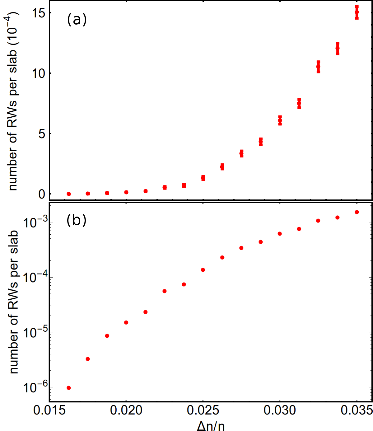
Figure 5: (a) The mean number of RWs per simulated slab as a function of the normalized refractive index fluctuation contrast $\Delta n/n$ is shown, where the correlation length of $\mu=2.8\lambda$ is assumed. The error bars are the standard error calculated for a sample size of 5,000 at each point; (b) Identical to (a), except plotted in a logarithmic scale.

The results presented in Fig. 5 are for in-plane fluctuations. In reality, the refractive index fluctuations occur in the full volume; therefore, one expects that the number of RWs in a sample with fluctuations in three dimensions ($N_{3}$) scale as $N_{3}\propto N_{2}^{3/2}$, where $N_{2}$ is the number of RWs in a sample with only in-plane fluctuations. Considering that the area of each sample here is assumed to be $10^{4}\lambda^{2}$, one can readily estimate the mean number of RWs generated per $\lambda^{3}$ volume element in the presence of the correlated refractive index fluctuations in 3D. The result is plotted in Fig. 6, which is extracted from Fig. 5(b), where the number of RWs is divided by $10^{4}$ to find the number of in-plane RWs per $\lambda^{2}$ area and subsequently raised to the power $3/2$ to find the expected number of RWs per $\lambda^{3}$ volume.

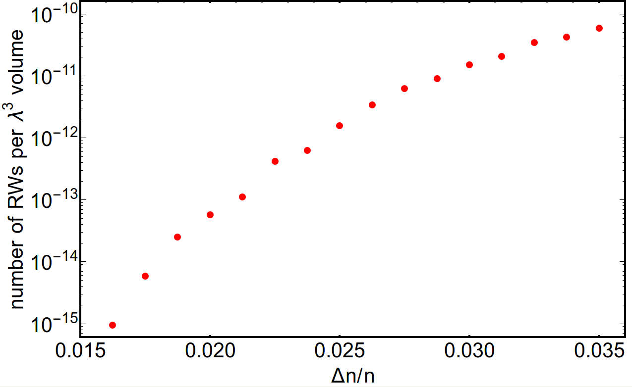
Figure 6: The mean number of RWs per $\lambda^{3}$ volume as a function of the normalized refractive index fluctuation contrast $\Delta n/n$ is shown, where the correlation length of $\mu=2.8\lambda$ is assumed.

Figure 6 shows that for $\Delta n\approx 0.02$, the mean number of RWs per $\lambda^{3}$ volume is on the order of $10^{-15}$. Therefore, for visible wavelength with $\lambda\approx 500$ nm, the mean number of RWs generated in a sample of 1 cm³ volume is approximately 0.01. In optical glasses, the nominal value for refractive index fluctuations is around $\Delta n\approx 0.00001$ or less. Figure 6 indicates that the probability for RW generation at such small refractive index fluctuations is quite small. Therefore, RWs are likely not responsible for the premature failure of optical materials below their nominal optical damage threshold in the bulk. However, it is possible that the presence of contaminants on optical surfaces such as dust, water, and skin oils, or imperfect polishing provide sufficient phase fluctuation on the surface to create hot spots as RWs near the surface, resulting in a lower damage threshold. It must be noted that the discussions in this Letter are exclusively on RW generation according to the definition of Method 2 and it is quite possible that refractive index fluctuations of around $\Delta n\approx 0.00001$ can still result in intensity peaks that do not qualify as a RW but can still contribute to the premature optical material failure.

IV Conclusion

We have shown that the presence of spatial correlation in the fluctuations of the refractive index of a dielectric media has an impact on the probability of rogue wave generation. In the examples that we explored in this Letter, we observed that by increasing the correlation length, the likelihood of rogue wave generation increases. A possible explanation for this behavior is that the presence of a spatial correlation result in an underlying structure that mimics a photonic crystal, in which the rogue waves are created as a coherent enhancement of amplitude due to a Bragg-type scattering behavior Chutinan:99 ; Mafi:15 . Our examples are generic; therefore, we believe our conclusions can be broadly applied to all coherent wave systems.

References

- (1) P. Müller, C. Garrett, and A. Osborne, “Rogue waves,” Oceanography 18, 66 (2005).
- (2) D. Solli, C. Ropers, P. Koonath, and B. Jalali, “Optical rogue waves,” Nature 450, 1054–1057 (2007).
- (3) F. Arecchi, U. Bortolozzo, A. Montina, and S. Residori, “Granularity and inhomogeneity are the joint generators of optical rogue waves,” Phys. Rev. Lett. 106, 153901 (2011).
- (4) N. Akhmediev and E. Pelinovsky, “Editorial–Introductory remarks on discussion and debate: Rogue waves–towards a unifying concept?,” Eur. Phys. J. Special Topics 185, 1–4 (2010).
- (5) M. Leonetti and C. Conti, “Observation of three dimensional optical rogue waves through obstacles,” Appl. Phys. Lett. 106, 254103 (2015).
- (6) A. Safari, R. Fickler, M. J. Padgett, and R. W. Boyd, “Generation of Caustics and Rogue Waves from Nonlinear Instability,” Phys. Rev. Lett. 119, 203901 (2017).
- (7) C. Lafargue, J. Bolger, G. Genty, F. Dias, J. Dudley, and B. Eggleton, “Direct detection of optical rogue wave energy statistics in supercontinuum generation,” Electron. Lett. 45, 217–219 (2009).
- (8) D. Solli, B. Jalali, and C. Ropers, “Seeded supercontinuum generation with optical parametric down-conversion,” Phys. Rev. Lett. 105, 233902 (2010).
- (9) D. Buccoliero, H. Steffensen, H. Ebendorff-Heidepriem, T. M. Monro, and O. Bang, “Midinfrared optical rogue waves in soft glass photonic crystal fiber,” Opt. Express 19, 17973–17978 (2011).
- (10) A. Montina, U. Bortolozzo, S. Residori, and F. Arecchi, “Non-Gaussian statistics and extreme waves in a nonlinear optical cavity,” Phys. Rev. Lett. 103, 173901 (2009).
- (11) S. Residori, U. Bortolozzo, A. Montina, F. Lenzini, and F. Arecchi, “Rogue waves in spatially extended optical systems,” Fluctuation Noise Lett. 11, 1240014 (2012).
- (12) C. Finot, K. Hammani, J. Fatome, J. M. Dudley, and G. Millot, “Selection of extreme events generated in raman fiber amplifiers through spectral offset filtering,” IEEE J. Quantum Electron. 46, 205–213 (2010).
- (13) K. Hammani and C. Finot, “Experimental signatures of extreme optical fluctuations in lumped raman fiber amplifiers,” Opt. Fiber Tech. 18, 93–100 (2012).
- (14) R. Höhmann, U. Kuhl, H.-J. Stöckmann, L. Kaplan, and E. Heller, “Freak waves in the linear regime: A microwave study,” Phys. Rev. Lett. 104, 093901 (2010).
- (15) L. Ying, Z. Zhuang, E. Heller, and L. Kaplan, “Linear and nonlinear rogue wave statistics in the presence of random currents,” Nonlinearity 24, R67 (2011).
- (16) M. Mattheakis, I. Pitsios, G. Tsironis, and S. Tzortzakis, “Extreme events in complex linear and nonlinear photonic media,” Chaos, Solitons & Fractals 84, 73–80 (2016).
- (17) M. Peysokhan, E. Mobini, J. Keeney, and A. Mafi, “Optical rouge wave generation in dielectrics with correlated fluctuations of refractive index,” in “Frontiers in Optics,” (Optical Society of America, 2017), pp. JW4A–111.
- (18) W. Rudolph, L. Emmert, Z. Sun, D. Patel, and C. Menoni, “Laser damage in dielectric films: What we know and what we don’t,” in “Laser-Induced Damage in Optical Materials: 2013,” (International Society for Optics and Photonics, 2013), vol. 8885, p. 888516.
- (19) A. Taflove, A. Oskooi, and S. G. Johnson, Advances in FDTD computational electrodynamics: photonics and nanotechnology (Artech house, Norwood, MA, 2013).
- (20) A. F. Oskooi, D. Roundy, M. Ibanescu, P. Bermel, J. D. Joannopoulos, and S. G. Johnson, “Meep: A flexible free-software package for electromagnetic simulations by the fdtd method,” Comput. Phys. Commun. 181, 687–702 (2010).
- (21) A. Mafi, “Transverse Anderson localization of light: a tutorial,” Adv. Opt. Photonics 7, 459–515 (2015).
- (22) M. S. Longuet-Higgins and G. E. R. Deacon, “The statistical analysis of a random, moving surface,” Philos. Trans. Royal Soc. A: Mathematical, Physical and Engineering Sciences 249, 321–387 (1957).
- (23) J. M. Dudley, F. Dias, M. Erkintalo, and G. Genty, “Instabilities, breathers and rogue waves in optics,” Nat. Photonics 8, 755 (2014).
- (24) A. Chutinan and S. Noda, “Effects of structural fluctuations on the photonic bandgap during fabrication of a photonic crystal: a study of a photonic crystal with a finite number of periods,” J. Opt. Soc. Am. 16, 1398–1402 (1999).
- (25) A. Mafi, “Anderson localization in a partially random Bragg grating and a conserved area theorem,” Opt. Lett. 40, 3603–3606 (2015).