Periodic thermodynamics of the Rabi model with circular polarization
for arbitrary spin quantum numbers

Abstract

We consider a spin $s$ subjected to both a static and an orthogonally applied oscillating, circularly polarized magnetic field while being coupled to a heat bath, and analytically determine the quasistationary distribution of its Floquet-state occupation probabilities for arbitrarily strong driving. This distribution is shown to be Boltzmannian with a quasitemperature which is different from the temperature of the bath, and independent of the spin quantum number. We discover a remarkable formal analogy between the quasithermal magnetism of the nonequilibrium steady state of a driven ideal paramagnetic material, and the usual thermal paramagnetism. Nonetheless, the response of such a material to the combined fields is predicted to show several unexpected features, even allowing one to turn a paramagnet into a diamagnet under strong driving. Thus, we argue that experimental measurements of this response may provide key paradigms for the emerging field of periodic thermodynamics.

I Introduction

A quantum system governed by an explicitly time-dependent Hamiltonian $H(t)$ which varies periodically with time $t$, such that

$$H(t)=H(t+T)\;,$$ (1)

possesses a complete set of Floquet states, that is, of solutions to the time-dependent Schrödinger equation having the particular form

$$|\psi_{n}(t)\rangle=|u_{n}(t)\rangle\exp(-{\mathrm{i}}\varepsilon_{n}t)\;.$$ (2)

The Floquet functions $|u_{n}(t)\rangle$ share the $T$-periodic time dependence of their Hamiltonian,

$$|u_{n}(t)\rangle=|u_{n}(t+T)\rangle\;;$$ (3)

the quantities $\varepsilon_{n}$, which accompany their time evolution in the same manner as energy eigenvalues accompany the evolution of unperturbed energy eigenstates, are known as quasienergies Zeldovich66 ; Sambe73 ; FainshteinEtAl78 . Here we assume that the quasienergies constitute a pure point spectrum, associated with square-integrable Floquet states in the system’s Hilbert space ${\mathcal{H}}_{S}$; we also adopt a system of units such that both the Planck constant $\hbar$ and the Boltzmann constant $k_{\rm B}$ are set to one.

Evidently the factorization of a Floquet state (2) into a Floquet function and an exponential of a phase which grows linearly in time is not unique: Defining $\omega=2\pi/T$, and taking an arbitrary, positive or negative integer $\nu$, one has

$$|u_{n}(t)\rangle\exp(-{\mathrm{i}}\varepsilon_{n}t)=|u_{n}(t){\mathrm{e}}^{{\mathrm{i}}\nu\omega t}\rangle\exp\!\big{(}-{\mathrm{i}}[\varepsilon_{n}+\nu\omega]t\big{)}\;,$$ (4)

where $|u_{n}(t){\mathrm{e}}^{{\mathrm{i}}\nu\omega t}\rangle$ again is a $T$-periodic Floquet function, representing the same Floquet state as $|u_{n}(t)\rangle$. Therefore, a quasienergy is not to be regarded as just a single number equipped with the dimension of energy, but rather as an infinite set of equivalent representatives,

$$[\varepsilon_{n}]\equiv\{\varepsilon_{n}+\nu\omega\;|\;\nu\in{\mathbbm{Z}}\}\;,$$ (5)

where the choice of the “canonical representative” distinguished by setting $\nu=0$ is a matter of convention.

The significance of these Floquet states (2) rests in the fact that, as long as the Hamiltonian depends on time in a strictly $T$-periodic manner, every solution $|\psi(t)\rangle$ to the time-dependent Schrödinger equation can be expanded with respect to the Floquet basis,

$$|\psi(t)\rangle=\sum_{n}c_{n}\,|u_{n}(t)\rangle\exp(-{\mathrm{i}}\varepsilon_{n}t)\;,$$ (6)

where the coefficients $c_{n}$ do not depend on time. Hence, the Floquet states propagate with constant occupation probabilities $|c_{n}|^{2}$, despite the presence of a time-periodic drive. Under conditions of perfectly coherent time evolution these coefficients $c_{n}$ would be determined solely by the system’s state at the moment the periodic drive is turned on. However, if the periodically driven system is interacting with an environment, as it happens in many cases of experimental interest BlumelEtAl91 ; GrifoniHanggi98 ; GasparinettiEtAl13 ; StaceEtAl13 ; ZhangEtAl17 ; ChoiEtAl17 , that environment may continuously induce transitions among the system’s Floquet states, to the effect that a quasistationary distribution $\{p_{n}\}$ of Floquet-state occupation probabilities establishes itself which contains no memory of the initial state, and the question emerges how to quantify this distribution.

In a short programmatic note entitled “Periodic Thermodynamics”, Kohn has drawn attention to such quasistationary Floquet-state distributions $\{p_{n}\}$, emphasizing that they should be less universal than usual distributions characterizing thermal equilibrium, depending on the very form of the system’s interaction with its environment Kohn01 . In an earlier pioneering study, Breuer et al. had already calculated these distributions for time-periodically forced oscillators coupled to a thermal oscillator bath BreuerEtAl00 . For the particular case of a linearly forced harmonic oscillator these authors have shown that the Floquet-state distribution remains a Boltzmann distribution parametrized by the temperature of the heat bath, whereas it becomes rather more complicated in the case of forced anharmonic oscillators. These investigations have been extended later by Ketzmerick and Wustmann, who have demonstrated that structures found in the phase space of classical forced anharmonic oscillators leave their distinct traces in the quasistationary Floquet-state distributions of their quantum counterparts KetzmerickWustmann10 . To date, a great variety of different individual aspects of the “periodic thermodynamics” envisioned by Kohn has been discussed in the literature HoneEtAl09 ; BulnesCuetaraEtAl15 ; ShiraiEtAl15 ; Liu15 ; IadecolaEtAl15a ; IadecolaEtAl15 ; SeetharamEtAl15 ; VorbergEtAl15 ; VajnaEtAl16 ; RestrepoEtAl16 ; LazaridesMoessner17 ; SeetharamEtAl19 , but a coherent overall picture is still lacking.

In this situation it seems advisable to resort to models which are sufficiently simple to admit analytical solutions and thus to unravel salient features on the one hand, and which actually open up meaningful perspectives for groundbreaking novel laboratory experiments on the other. To this end, in the present work we consider a spin $s$ exposed to both a static magnetic field and an oscillating, circularly polarized magnetic field applied perpendicularly to the static one, as in the classic Rabi set-up Rabi37 , and coupled to a thermal bath of harmonic oscillators. The experimental measurement of the thermal paramagnetism resulting from magnetic moments subjected to a static field alone has a long and successful history Brillouin27 ; Henry52 , having become a standard topic in textbooks on Statistical Physics FowlerGuggenheim39 ; Pathria11 . We argue that a future generation of such experiments, including both a static and a strong oscillating field, may set further milestones towards the development of full-fledged periodic thermodynamics.

We proceed as follows: In Sec. II we collect the necessary technical tools, starting with a brief summary of the golden-rule approach to time-periodically driven open quantum systems in the form developed by Breuer et al. BreuerEtAl00 , thereby establishing our notation. We also sketch a technique which enables one to “lift” a solution to the Schrödinger equation for a spin $s=1/2$ in a time-varying magnetic field to general $s$. In Sec. III we discuss the Floquet states for spins in a circularly polarized driving field, obtaining the states for general $s$ from those for $s=1/2$ with the help of the lifting procedure. In Sec. IV we compute the quasistationary Floquet-state distribution for driven spins under the assumption that the spectral density of the heat bath be constant, and show that this distribution is Boltzmannian with a quasitemperature which is different from the actual bath temperature; the dependence of this quasitemperature on the system parameters is discussed in some detail. In Sec. V we determine the magnetization of a spin system which is subjected to both a static and an orthogonally applied, circularly polarized magnetic field while being coupled to a heat bath. To this end, we first establish a general formula for the ensuing magnetization by means of another systematic use of the lifting technique, and then show that the resulting expression can be interpreted as a derivative of a partition function based on both the quasitemperature and the system’s quasienergies, in perfect formal analogy to the textbook treatment of paramagnetism in the absence of time-periodic driving; these insights are exploited for elucidating the response of an ideal paramagnet to a circularly polarized driving field. In Sec. VI we consider the rate of energy dissipated by the driven spins into the bath, thus generalizing results derived previously for $s=1/2$ in Ref. LangemeyerHolthaus14 . In Sec. VII we summarize and discuss our main findings, emphasizing the possible knowledge gain to be derived from future measurements of paramagnetic response to strong time-periodic forcing, carried out along the lines drawn in the present work.

II Technical Tools

II.1 Golden-rule approach to open driven systems

Let us consider a quantum system evolving according to a $T$-periodic Hamiltonian $H(t)$ on a Hilbert space ${\mathcal{H}}_{S}$ which is perturbed by a time-independent operator $V$. Then the transition matrix element connecting an initial Floquet function $|u_{i}(t)\rangle$ to a final Floquet function $|u_{f}(t)\rangle$ can be expanded into a Fourier series,

$$\langle u_{f}(t)|\,V\,|u_{i}(t)\rangle=\sum_{\ell\in{\mathbbm{Z}}}\,V_{fi}^{(\ell)}\exp({\mathrm{i}}\ell\omega t)\;,$$ (7)

and consequently the “golden rule” for the rate of transitions $\Gamma_{fi}$ from a Floquet state labeled $i$ to a Floquet state $f$ is written as LangemeyerHolthaus14

$$\Gamma_{fi}=2\pi\sum_{\ell\in{\mathbbm{Z}}}\,|V_{fi}^{(\ell)}|^{2}\,\delta(\omega_{fi}^{(\ell)})\;,$$ (8)

where

$$\omega_{fi}^{(\ell)}=\varepsilon_{f}-\varepsilon_{i}+\ell\omega\;.$$ (9)

Thus, a transition among Floquet states is not simply associated with only one single frequency, but rather with a set of frequencies spaced by integer multiples of the driving frequency $\omega$, reflecting the ladder-like nature of the system’s quasienergies (5); this is one of the sources of the peculiarities which distinguish periodic thermodynamics from usual equilibrium thermodynamics Kohn01 ; BreuerEtAl00 .

Let us now assume that, instead of merely being perturbed by $V$, the periodically driven system is coupled to a heat bath, described by a Hamiltonian $H_{\rm bath}$ acting on a Hilbert space ${\mathcal{H}}_{B}$, so that the total Hamiltonian on the composite Hilbert space ${\mathcal{H}}_{S}\otimes{\mathcal{H}}_{B}$ takes the form

$$H_{\rm total}(t)=H(t)\otimes{\mathbbm{1}}+{\mathbbm{1}}\otimes H_{\rm bath}+H_{\rm int}\;.$$ (10)

Stipulating further that the interaction Hamiltonian $H_{\rm int}$ factorizes according to

$$H_{\rm int}=V\otimes W\;,$$ (11)

the golden rule can be applied to joint transitions from Floquet states $i$ to Floquet states $f$ of the system accompanied by transitions from bath eigenstates $n$ with energy $E_{n}$ to other bath eigenstates $m$ with energy $E_{m}$, acquiring the form

$$\Gamma_{fi}^{mn}=2\pi\sum_{\ell\in{\mathbbm{Z}}}\,|V_{fi}^{(\ell)}|^{2}\,|W_{mn}|^{2}\,\delta(E_{m}-E_{n}+\omega_{fi}^{(\ell)})\;.$$ (12)

Moreover, following Breuer et al. BreuerEtAl00 , let us consider a bath consisting of thermally occupied harmonic oscillators, and an interaction of the prototypical form

$$W=\sum_{\widetilde{\omega}}\left(b_{\widetilde{\omega}}^{\phantom{\dagger}}+b_{\widetilde{\omega}}^{\dagger}\right)\;,$$ (13)

where $b_{\widetilde{\omega}}^{\phantom{\dagger}}$ ($b_{\widetilde{\omega}}^{\dagger}$) is the annihilation (creation) operator pertaining to a bath oscillator of frequency $\widetilde{\omega}$. One could also multiply $W$ by a function $g(\widetilde{\omega})$ specifying a frequency-dependent coupling strength, but this function could be absorbed in the spectral density of the bath introduced later, and therefore will not be used here.

We now have to distinguish two cases: If $E_{n}-E_{m}=\widetilde{\omega}>0$, so that the bath is de-excited and transfers energy to the system, the required annihilation-operator matrix element reads

$$W_{mn}=\sqrt{n(\widetilde{\omega})}\;,$$ (14)

where $n(\widetilde{\omega})$ is the occupation number of a bath oscillator with frequency $\widetilde{\omega}$, and the square $|W_{mn}|^{2}$ entering the golden rule (12) has to be replaced by the thermal avarage

$$N(\widetilde{\omega})\equiv\langle n(\widetilde{\omega})\rangle=\frac{1}{\exp(\beta\widetilde{\omega})-1}\;,$$ (15)

with $\beta$ denoting the inverse bath temperature. Conversely, if $E_{n}-E_{m}=\widetilde{\omega}<0$ so that the system loses energy to the bath and a bath phonon is created, one has

$$W_{mn}=\sqrt{n(-\widetilde{\omega})+1}\;,$$ (16)

giving

$$N(\widetilde{\omega})\equiv\langle n(-\widetilde{\omega})\rangle+1=\frac{1}{1-\exp(\beta\widetilde{\omega})}\;.$$ (17)

Finally, let $J(\widetilde{\omega})$ be the spectral density of the bath. Then the total rate $\Gamma_{fi}$ of bath-induced transitions among the Floquet states $i$ and $f$ of the driven system is expressed as a sum of partial rates,

$$\Gamma_{fi}=\sum_{\ell\in{\mathbbm{Z}}}\,\Gamma_{fi}^{(\ell)}\;,$$ (18)

where

$$\Gamma_{fi}^{(\ell)}=2\pi\,|V_{fi}^{(\ell)}|^{2}\,N(\omega_{fi}^{(\ell)})\,J(|\omega_{fi}^{(\ell)}|)\;.$$ (19)

The evaluation of this formula requires a definite specification of the quasienergy representatives for each state when computing the transition frequencies (9); this specification also fixes the representatives of the Floquet functions which enter the matrix elements (7). An alternative choice of representatives would lead to a shift of the Fourier index $\ell$, but leaves the sum (18) invariant.

These total rates (18) now determine the desired quasistationary distribution $\{p_{n}\}$ as a solution to the equation BreuerEtAl00

$$\sum_{m}\big{(}\Gamma_{nm}p_{m}-\Gamma_{mn}p_{n}\big{)}=0\;.$$ (20)

It deserves to be emphasized again that the very details of the system-bath coupling enter here, so that the precise form of the respective distribution $\{p_{n}\}$ may depend strongly on such details Kohn01 .

II.2 The lift from $s=1/2$ to general $s$

We will make heavy use of a procedure which allows one to transfer a solution to the Schrödinger equation for a spin with spin quantum number $s=1/2$ in a time-dependent external field to a solution of the corresponding Schrödinger equation for general $s$, see also Ref. Schmidt18 . This procedure essentially rests on the fact that a spin-$s$ state can be represented as a direct symmetrized product of $2s$ spin-$1/2$ states, as exposed by Landau and Lifshitz LaLiQM81 . It does not appear to be widely known, but has been applied already in 1987 to the coherent evolution of a laser-driven $N$-level system possessing an $SU(2)$ dynamic symmetry Hioe87 , and more recently to the spin-$s$ Landau-Zener problem PokrovskySinitsyn04 . Here we briefly sketch this method.

Let $t\mapsto\Psi(t)\in SU(2)$ be a smooth curve such that $\Psi(0)={\mathbbm{1}}$, as given by a $2\times 2$-matrix of the form

$$\Psi(t)=\left(\begin{array}[]{rr}z_{1}(t)&z_{2}(t)\\ -z_{2}^{\ast}(t)&z_{1}^{\ast}(t)\end{array}\right)$$ (21)

with complex functions $z_{1}(t)$, $z_{2}(t)$ obeying $|z_{1}(t)|^{2}+|z_{2}(t)|^{2}=1$ for all times $t$. One then has

$$\left(\frac{{\mathrm{d}}}{{\mathrm{d}}t}\Psi(t)\right)\,\Psi(t)^{-1}\equiv-{\mathrm{i}}H(t)\in su(2)\;,$$ (22)

where $su(2)$ denotes the Lie algebra of $SU(2)$, i.e., the space of anti-Hermitean, traceless $2\times 2$-matrices which is closed under commutation Hall15 . Hence the columns $|\psi_{1}(t)\rangle$, $|\psi_{2}(t)\rangle$ of $\Psi(t)$ are linearly independent solutions of the Schrödinger equation

$${\mathrm{i}}\frac{{\mathrm{d}}}{{\mathrm{d}}t}|\psi_{j}(t)\rangle=H(t)\,|\psi_{j}(t)\rangle\;,\quad j=1,2\;.$$ (23)

Next we consider the well-known irreducible Lie algebra representation of $su(2)$,

$$r^{(s)}:su(2)\longrightarrow su(2s+1)\;,$$ (24)

which is parametrized by a spin quantum number $s$ such that $2s\in{\mathbbm{N}}$, together with the corresponding irreducible group representation (“irrep” for brevity)

$$R^{(s)}:SU(2)\longrightarrow SU(2s+1)\;.$$ (25)

One then has Hall15

$$r^{(s)}({\mathrm{i}}s_{j})={\mathrm{i}}S_{j}\;,\quad j=x,y,z\;,$$ (26)

where $s_{j}=\sigma_{j}/2$ denote the three $s=1/2$ spin operators given by the Pauli matrices $\sigma_{j}$, and the $S_{j}$ denote the corresponding spin operators for general $s$. Recall the standard matrices

$$\left(S_{z}\right)_{m,n} = n\,\delta_{mn}\;,$$ (27)

$$\left(S_{x}\right)_{m,n} = \left\{\begin{array}[]{r@{\quad:\quad}l}\phantom{\pm}\displaystyle\frac{1}{2}\sqrt{s(s+1)-n(n\pm 1)}&m=n\pm 1\;,\\ 0&\mbox{else}\;,\end{array}\right.$$ (30)

$$\left(S_{y}\right)_{m,n} = \left\{\begin{array}[]{r@{\quad:\quad}l}\pm\displaystyle\frac{1}{2{\mathrm{i}}}\sqrt{s(s+1)-n(n\pm 1)}&m=n\pm 1\;,\\ 0&\mbox{else}\;,\end{array}\right.$$ (33)

where $m,n=s,s-1,\ldots,-s$, and

$$S_{\pm}\equiv S_{x}\pm{\mathrm{i}}S_{y}\;.$$ (34)

It follows from the general theory of representations Hall15 that $r^{(s)}$ and $R^{(s)}$ may be applied to Eq. (22) and yield

$$\left(\frac{{\mathrm{d}}}{{\mathrm{d}}t}R^{(s)}\,\Psi(t)\right)\,\left(R^{(s)}\,\Psi(t)\right)^{-1}=r^{(s)}\big{(}-{\mathrm{i}}H(t)\big{)}\;.$$ (35)

Since the traceless matrix $H(t)$ can always be written as a linear combination of the spin operators $s_{j}$ it acquires the form of a Zeeman term with a time-dependent magnetic field ${\mathbf{b}}(t)$, namely,

$$H(t)={\mathbf{b}}(t)\cdot{\mathbf{s}}=\sum_{j=1}^{3}b_{j}(t)\,s_{j}\;,$$ (36)

and Eq. (26) now implies

$$r^{(s)}\big{(}-{\mathrm{i}}H(t)\big{)}=-{\mathrm{i}}\,{\mathbf{b}}(t)\cdot{\mathbf{S}}=-{\mathrm{i}}\sum_{j=1}^{3}b_{j}(t)\,S_{j}\;.$$ (37)

Hence, the “lifted” matrix

$$\Psi^{(s)}(t)\equiv R^{(s)}\big{(}\Psi(t)\big{)}$$ (38)

will be a matrix solution to the lifted Schrödinger equation

$${\mathrm{i}}\frac{{\mathrm{d}}}{{\mathrm{d}}t}\Psi^{(s)}(t)={\mathbf{b}}(t)\cdot{\mathbf{S}}\,\Psi^{(s)}(t)\;.$$ (39)

Note that the matrix $\Psi^{(s)}(t)$ is unitary, and hence its columns span the general $(2s+1)$-dimensional solution space of the lifted Schrödinger equation (39). The decisive step of this procedure, namely, the lift from Eq. (22) to Eq. (35), is further illustrated in Appendix A with the help of an elementary example.

III Floquet formulation of the Rabi problem

III.1 Floquet decomposition for $s=1/2$

A spin $1/2$ subjected to both a constant magnetic field applied in the $z$-direction and an orthogonal, circularly polarized time-periodic field, as constituting the classic Rabi problem Rabi37 , is described by the Hamiltonian

$$H(t)=\frac{\omega_{0}}{2}\sigma_{z}+\frac{F}{2}(\sigma_{x}\cos\omega t+\sigma_{y}\sin\omega t)\;.$$ (40)

Here $\omega_{0}>0$ denotes the transition frequency pertaining to the spin states in the static field alone, while $F$, carrying the dimension of a frequency in our system of units, denotes the amplitude of the periodic drive. This is a special form of the Zeeman Hamiltonian (36) with the particular choices

$$b_{x}(t) = F\cos\omega t$$

$$b_{y}(t) = F\sin\omega t$$

$$b_{z}(t) = \omega_{0}\;.$$ (41)

The Floquet states (2) brought about by this Hamiltonian (40) are given by HolthausJust94

$$|\psi_{\pm}(t)\rangle=\frac{{\mathrm{e}}^{\mp{\mathrm{i}}\Omega t/2}}{\sqrt{2\Omega}}\left(\begin{array}[]{r}\pm\sqrt{\Omega\pm\delta}\;{\mathrm{e}}^{-{\mathrm{i}}\omega t/2}\\ \sqrt{\Omega\mp\delta}\;{\mathrm{e}}^{+{\mathrm{i}}\omega t/2}\end{array}\right)\;,$$ (42)

where

$$\delta=\omega_{0}-\omega$$ (43)

denotes the detuning of the transition frequency $\omega_{0}$ from the driving frequency $\omega$, and $\Omega$ is the Rabi frequency,

$$\Omega=\sqrt{\delta^{2}+F^{2}}\;.$$ (44)

The $2\times 2$-matrix $\Psi(t)$ constructed from these states does not satisfy $\Psi(0)={\mathbbm{1}}$. This is of no concern, since $\Psi(t)$ could be replaced by $\Psi(t)\big{(}\Psi(0)\big{)}^{-1}$. The distinct advantage of these Floquet solutions (42) lies in the fact that they yield a particularly convenient starting point for the lifting procedure outlined in Sec. II.2: One has

$$\Psi(t) = \frac{1}{\sqrt{2\Omega}}\left(\begin{array}[]{rr}\sqrt{\Omega+\delta}&-\sqrt{\Omega-\delta}\\ {\mathrm{e}}^{{\mathrm{i}}\omega t}\sqrt{\Omega-\delta}&{\mathrm{e}}^{{\mathrm{i}}\omega t}\sqrt{\Omega+\delta}\end{array}\right)$$ (50)

$$\times\left(\begin{array}[]{cc}{\mathrm{e}}^{-{\mathrm{i}}(\omega+\Omega)t/2}&0\\ 0&{\mathrm{e}}^{-{\mathrm{i}}(\omega-\Omega)t/2}\end{array}\right)$$

$$\equiv P(t)\,{\mathrm{e}}^{-{\mathrm{i}}\omega t/2}\,\exp(-{\mathrm{i}}\Omega t\,s_{z})\;.\phantom{\int_{a}^{b}}$$ (51)

This decomposition possesses the general Floquet form

$$\Psi(t)=P(t)\exp(-{\mathrm{i}}Gt)\;,$$ (52)

where the unitary matrix $P(t)=P(t+T)$ again is $T$-periodic, and the eigenvalues of the “Floquet matrix” $G$, to be obtained from the matrix logarithm of $\Psi(T)\big{(}\Psi(0)\big{)}^{-1}=\exp(-{\mathrm{i}}GT)$, provide the system’s quasienergies Shirley65 ; Salzman74 ; GesztesyMitter81 ; Holthaus16 . Since $G$ already is diagonal in this representation (51), the quasienergies of a spin $1/2$ driven by a circularly polarized field according to the Hamiltonian (40) can be read off immediately:

$$\varepsilon_{\pm}=\frac{\omega\pm\Omega}{2}\quad\bmod\omega\;,$$ (53)

satisfying $\varepsilon_{+}+\varepsilon_{-}=0\,\bmod\,\omega$. For later application we express the periodic part $P(t)$ of the decomposition (51) in the following way:

$$P(t) = {\mathrm{e}}^{{\mathrm{i}}\omega t/2}\left(\begin{array}[]{cc}{\mathrm{e}}^{-{\mathrm{i}}\omega t/2}&0\\ 0&{\mathrm{e}}^{+{\mathrm{i}}\omega t/2}\end{array}\right)$$ (59)

$$\times\frac{1}{\sqrt{2\Omega}}\left(\begin{array}[]{rr}\sqrt{\Omega+\delta}&-\sqrt{\Omega-\delta}\\ \sqrt{\Omega-\delta}&\sqrt{\Omega+\delta}\end{array}\right)$$

$$\equiv {\mathrm{e}}^{{\mathrm{i}}\omega t/2}\exp(-{\mathrm{i}}\omega t\,s_{z})\,\Xi\;.\phantom{\int_{a}^{b}}$$ (60)

The time-independent matrix $\Xi=\Psi(0)$ introduced here can be written as

$$\Xi=\exp\left(-{\mathrm{i}}\lambda\,s_{y}\right)=\left(\begin{array}[]{rr}\cos(\lambda/2)&-\sin(\lambda/2)\\ \sin(\lambda/2)&\cos(\lambda/2)\end{array}\right)$$ (61)

with

$$\lambda/2=\arccos\left(\sqrt{\frac{\Omega+\delta}{2\Omega}}\right)\;.$$ (62)

Hence, one has the identities

$$\Xi^{\dagger}s_{x}\Xi = \frac{\delta}{\Omega}\,s_{x}+\frac{\sqrt{\Omega^{2}-\delta^{2}}}{\Omega}\,s_{z}$$

$$\Xi^{\dagger}s_{y}\Xi = s_{y}\phantom{\frac{\delta}{\Omega}}\;,$$

$$\Xi^{\dagger}s_{z}\Xi = \frac{\delta}{\Omega}\,s_{z}-\frac{\sqrt{\Omega^{2}-\delta^{2}}}{\Omega}\,s_{x}\;,$$ (63)

which will be put into use in both Sec. IV and Sec. V.

III.2 Floquet decomposition for general $s$

Replacing the spin-$1/2$ operators $s_{j}=\sigma_{j}/2$ in the Hamiltonian (40) by their conterparts $S_{j}$ for general spin quantum number $s$, one obtains

$$H^{(s)}(t) = {\mathbf{b}}(t)\cdot{\mathbf{S}}$$ (64)

$$= \omega_{0}\,S_{z}+F\left(S_{x}\,\cos\omega t+S_{y}\,\sin\omega t\right)\;.$$

According to Sec. II.2 the general matrix solution to the corresponding Schrödinger equation (39) now is obtained as the lift (38) of the $2\times 2$-matrix (51). Invoking Eqs. (60) and (61), and applying the irrep $R^{(s)}$ to this decomposition yields

$$\Psi^{(s)}(t) = R^{(s)}\!\Big{(}\exp(-{\mathrm{i}}\omega t\,s_{z})\exp\left(-{\mathrm{i}}\lambda\,s_{y}\right)\exp(-{\mathrm{i}}\Omega t\,s_{z})\Big{)}$$ (65)

$$= \exp(-{\mathrm{i}}\omega t\,S_{z})\exp\left(-{\mathrm{i}}\lambda\,S_{y}\right)\exp(-{\mathrm{i}}\Omega t\,S_{z})\;.\phantom{\int_{a}^{b}}$$

In order to bring this factorization into the standard Floquet form analogous to Eq. (52),

$$\Psi^{(s)}(t)=P^{(s)}(t)\exp\!\big{(}-{\mathrm{i}}G^{(s)}t\big{)}$$ (66)

with a $T$-periodic matrix $P^{(s)}(t)=P^{(s)}(t+T)$, we have to distinguish two cases:

(i)

For integer $s$ we may set

$$P^{(s)}(t) = \exp(-{\mathrm{i}}\omega t\,S_{z})\,\exp\left(-{\mathrm{i}}\lambda\,S_{y}\right)\;,$$

$$G^{(s)} = \Omega\,S_{z}\;.$$ (67)

(ii)

For half-integer $s$ the requirement that $P^{(s)}(t)$ be $T$-periodic demands insertion of additional factors ${\mathrm{e}}^{\pm{\mathrm{i}}\omega t/2}$, in analogy to the representation (60) for $s=1/2$. This gives

$$P^{(s)}(t) = {\mathrm{e}}^{{\mathrm{i}}\omega t/2}\exp(-{\mathrm{i}}\omega t\,S_{z})\,\exp\left(-{\mathrm{i}}\lambda\,S_{y}\right)\;,$$

$$G^{(s)} = \frac{\omega}{2}{\mathbbm{1}}^{(s)}+\Omega\,S_{z}\;,$$ (68)

where ${\mathbbm{1}}^{(s)}$ indicates the unit matrix in ${\mathbbm{C}}^{2s+1}$.

Denoting the eigenstates of $S_{z}$ as $|m\rangle$, such that $S_{z}|m\rangle=m|m\rangle$, we now introduce Floquet functions and their quasienergies according to the prescription

$$\Psi^{(s)}(t)\,|m\rangle = P^{(s)}(t)\,|m\rangle\,\exp\!\left(-{\mathrm{i}}\varepsilon_{m}t\right)$$ (69)

$$\equiv |u_{m}(t)\rangle\,\exp\!\left(-{\mathrm{i}}\varepsilon_{m}t\right)\;,$$

implying the particular choice

$$|u_{m}(t)\rangle=P^{(s)}(t)\,|m\rangle$$ (70)

of $T$-periodic Floquet functions. The associated quasienergy representatives then are

$$\varepsilon_{m}=m\Omega$$ (71)

for integer $s$ according to case (i), or

$$\varepsilon_{m}=\frac{\omega}{2}+m\Omega$$ (72)

for half-integer $s$ according to case (ii), with $m=-s,\ldots,s$. This convenient choice of representatives will be presupposed in the following for computing the partial rates (19). Observe that there is a further, physically important distinction to be made at this point: When the driving amplitude vanishes, that is, for $F\to 0$, the Rabi frequency (44) does not reduce to the detuning, but rather to the absolute value of the detuning, $\Omega\to|\omega_{0}-\omega|$. Hence, for $F\to 0$ the Floquet functions (70) “connect” to $|m\rangle$ only for red detuning, when $\omega<\omega_{0}$, but to $|-m\rangle$ for blue detuning, when $\omega>\omega_{0}$. Hence, under blue detuning the labeling of the Floquet functions and their quasienergies effectively is reversed with respect to the eigenstates of $S_{z}$. This feature needs to be kept in mind for correctly assessing the following results.

We also note that in the adiabatic low-frequency limit, when the spin is exposed to an arbitrarily slowly varying magnetic field enabling adiabatic following to the instantaneous energy eigenstates, the quasienergies should be given by the one-cyle averages of the instantaneous energy eigenvalues. Indeed, in this limit the Rabi frequency (44) reduces to $\Omega=\sqrt{\omega_{0}^{2}+F^{2}}$, while the time-independent instantaneous energy levels are $E_{m}=m\,\Omega$, yielding the expected identity.

IV The quasistationary distribution

Now we stipulate that the periodically driven spin be coupled to a thermal bath of harmonic oscillators, as sketched in Sec. II.1, taking the coupling operator to be of the simple form ExplainV

$$V=\gamma\,S_{x}\;.$$ (73)

In order to calculate the Fourier decompositions (7) of the Floquet matrix elements of $V$, and referring to the above representation (70) of the Floquet functions, we thus need to consider the operator

$$P^{(s)\dagger}(t)\,S_{x}\,P^{(s)}(t)$$ (74)

$$= \exp\left({\mathrm{i}}\lambda\,S_{y}\right)\exp\left({\mathrm{i}}\omega t\,S_{z}\right)\,S_{x}\,\exp\left(-{\mathrm{i}}\omega t\,S_{z}\right)\exp\left(-{\mathrm{i}}\lambda\,S_{y}\right)$$

$$\equiv \sum_{\ell\in{\mathbbm{Z}}}\,V^{(\ell)}\exp({\mathrm{i}}\ell\omega t)\;;$$

note that the additional phase factor ${\mathrm{e}}^{{\mathrm{i}}\omega t/2}$ contained in the expression (68) for $P^{(s)}(t)$ with half-integer $s$ cancels here. Using the $su(2)$ commutation relations and their counterparts for general $s$, we deduce

$$\exp\left({\mathrm{i}}\omega t\,S_{z}\right)\,S_{x}\,\exp\left(-{\mathrm{i}}\omega t\,S_{z}\right)$$ (75)

$$= \frac{1}{2}\left({\mathrm{e}}^{{\mathrm{i}}\omega t}\,S_{+}+{\mathrm{e}}^{-{\mathrm{i}}\omega t}\,S_{-}\right)\;.$$

Hence, as in the case $s=1/2$ studied in Ref. LangemeyerHolthaus14 , the only non-vanishing Fourier components $V^{(\ell)}$ occur for $\ell=\pm 1$:

$$V^{(\pm 1)}=\frac{\gamma}{2}\exp\left({\mathrm{i}}\lambda\,S_{y}\right)S_{\pm}\exp\left(-{\mathrm{i}}\lambda\,S_{y}\right)\;.$$ (76)

Applying $R^{(s)}$ to Eqs. (63), this yields

$$V^{(\pm 1)}=\frac{\gamma}{2}\left(\frac{\delta}{\Omega}\,S_{x}\,+\frac{\sqrt{\Omega^{2}-\delta^{2}}}{\Omega}\,S_{z}\,\pm{\mathrm{i}}\,S_{y}\right)\;.$$ (77)

Thus, $V^{(\pm 1)}$ is a tridiagonal matrix. For computing the partial transition rates (19) we therefore have to consider only frequencies $\omega_{mn}^{(\pm 1)}$ of pseudotransitions LangemeyerHolthaus14 , for which $m=n$, and of transitions between neighboring Floquet states, $m=n\pm 1$. For evaluating the definition (9) one now has to resort to the quasienergy representatives (71) and (72) which belong to the Floquet functions (70) entering here, giving

$$\omega_{mn}^{(\pm 1)}=\left\{\begin{array}[]{r@{\quad:\quad}l}\pm\omega&m=n\;,\\ \phantom{-}\Omega\pm\omega&m=n+1\;,\\ -\Omega\pm\omega&m=n-1\;.\end{array}\right.$$ (78)

According to the Pauli master equation (20), the quasistationary distribution $\{p_{m}\}_{m=s,\ldots,-s}$ which establishes itself under the combined influence of time-periodic driving and the thermal oscillator bath is the eigenvector of a tridiagonal matrix $\widetilde{\Gamma}$ corresponding to the eigenvalue $0$, where $\widetilde{\Gamma}$ is obtained from $\Gamma\equiv\Gamma^{(1)}+\Gamma^{(-1)}$ by subtracting from the diagonal elements the respective column sums, i.e.,

$$\widetilde{\Gamma}_{mn}=\Gamma_{mn}-\delta_{mn}\sum_{k=-s}^{s}\Gamma_{kn}\;.$$ (79)

Since $\widetilde{\Gamma}$ is tridiagonal with non-vanishing secondary diagonal elements, this eigenvector is unique up to normalization. Moreover, it is evident that we only need the matrix elements of $\Gamma$ in the secondary diagonals for calculating the quasistationary distribution, whereas the diagonal elements will be required for computing the dissipation rate LangemeyerHolthaus14 .

The very fact that $V^{(\pm 1)}$, and hence $\Gamma$, merely is a tridiagonal matrix has a conceptually important consequence: It enforces detailed balance, meaning that each term of the sum (20) vanishes individually. With $\Gamma$ being tridiagonal, this sum reduces to

$$(\Gamma_{n,n-1}\,p_{n-1}-\Gamma_{n-1,n}\,p_{n})$$

$$+\;(\Gamma_{n,n+1}\,p_{n+1}-\Gamma_{n+1,n}\,p_{n}) = 0$$ (80)

for all $n=-s+1$, $\ldots\,$, $s-1$, since the term with $m=n$ in Eq. (20) cancels. In the border cases $n=-s$ or $n=s$ this identity still holds, but only one bracket survives. Upon setting the first bracket in this Eq. (80) to zero, one obtains

$$\frac{p_{n}}{p_{n-1}}=\frac{\Gamma_{n,n-1}}{\Gamma_{n-1,n}}$$ (81)

for $n=-s+1$, $\ldots\,$, $s-1$. Together with the normalization requirement, this relation alone already determines the entire distribution $\{p_{m}\}$. In particular, it entails

$$\frac{p_{n+1}}{p_{n}}=\frac{\Gamma_{n+1,n}}{\Gamma_{n,n+1}}\;,$$ (82)

thus ensuring that also the second bracket in Eq. (80) vanishes, confirming detailed balance.

Now one needs to observe that the sign of the transition frequencies (78) depends on the relative magnitude of the driving frequency $\omega$ and the Rabi frequency $\Omega$; recall that the distinction between positive and negative transition frequencies — physically corresponding to the distinction between annihilation and creation of bath phonons — leads to the two different expressions (15) and (17) entering the transition rates (19). This prompts us to distinguish between the low-frequency case $0<\omega<\Omega$ and the high-frequency case $0<\Omega<\omega$ in the following. The resonant case $\omega=\Omega$ constitutes a special problem; this is best dealt with by taking the appropriate limits of the results obtained in the other two cases.

Finally, a further factor of substantial importance is the spectral density $J(\widetilde{\omega})$, which may allow one to manipulate the quasistationary distribution to a considerable extent DiermannEtAl19 . For the sake of simplicity and transparent discussion, here we assume that $J(\widetilde{\omega})\equiv J_{0}$ is constant.

IV.1 Low-frequency case $0<\omega<\Omega$

In order to utilize the above Eq. (82) for determining the distribution $\{p_{m}\}$ recursively we only need to evaluate the partial rates $\Gamma_{m,m+1}^{(\pm 1)}$ and $\Gamma_{m+1,m}^{(\pm 1)}$ according to the general prescription (19), making use of the particular representation (77). In the low-frequency case this leads to the expressions

$$\Gamma^{(\pm 1)}_{m,m+1} = \frac{s(s+1)-m(m+1)}{16\left(1-{\mathrm{e}}^{-\beta(\Omega\mp\omega)}\right)}\left(\frac{\Omega\mp\delta}{\Omega}\right)^{2}$$

$$\Gamma^{(\pm 1)}_{m+1,m} = \frac{s(s+1)-m(m+1)}{16\left({\mathrm{e}}^{\beta(\Omega\pm\omega)}-1\right)}\left(\frac{\Omega\pm\delta}{\Omega}\right)^{2}$$ (83)

which have been scaled by $\Gamma_{0}=2\pi\gamma^{2}J_{0}$, and have thus been made dimensionless. Evidently, these representations imply that the desired ratio

$$\frac{\Gamma_{m+1,m}}{\Gamma_{m,m+1}}\equiv q_{L}$$ (84)

is independent of both $s$ and $m$; a tedious but straightforward calculation readily yields

$$q_{L}=\frac{2\delta\Omega\sinh(\beta\omega)+\left(\delta^{2}+\Omega^{2}\right)\left({\mathrm{e}}^{-\beta\Omega}-\cosh(\beta\omega)\right)}{2\delta\Omega\sinh(\beta\omega)-\left(\delta^{2}+\Omega^{2}\right)\left({\mathrm{e}}^{\beta\Omega}-\cosh(\beta\omega)\right)}\;.$$ (85)

Therefore, the quasistationary occupation probabilities of the Floquet states can be written in the form

$$p_{m}=\frac{1}{Z_{L}}q_{L}^{m}$$ (86)

with $m=-s,\ldots,s$, and $Z_{L}$ ensuring normalization. Hence, not only does one find detailed balance here, but the occupation probabilities even generate a finite geometric sequence.

IV.2 High-frequency case $0<\Omega<\omega$

Analogously, in the high-frequency case $0<\Omega<\omega$ we require the dimensionless partial rates

$$\Gamma^{(\pm 1)}_{m,m+1} = \pm\frac{s(s+1)-m(m+1)}{16\left({\mathrm{e}}^{\beta(\pm\omega-\Omega)}-1\right)}\left(\frac{\Omega\mp\delta}{\Omega}\right)^{2}$$

$$\Gamma^{(\pm 1)}_{m+1,m} = \pm\frac{s(s+1)-m(m+1)}{16\left({\mathrm{e}}^{\beta(\Omega\pm\omega)}-1\right)}\left(\frac{\Omega\pm\delta}{\Omega}\right)^{2}$$ (87)

for constructing the matrix $\Gamma=\Gamma^{(1)}+\Gamma^{(-1)}$. Once more, the ratio

$$\frac{\Gamma_{m+1,m}}{\Gamma_{m,m+1}}\equiv q_{H}$$ (88)

does depend neither on $s$ nor on $m$, so that the occupation probabilities again form a geometric sequence; after some juggling, one finds

$$q_{H}=\frac{\left(\delta^{2}+\Omega^{2}\right)\sinh(\beta\omega)+2\delta\Omega\left({\mathrm{e}}^{-\beta\Omega}-\cosh(\beta\omega)\right)}{\left(\delta^{2}+\Omega^{2}\right)\sinh(\beta\omega)-2\delta\Omega\left({\mathrm{e}}^{\beta\Omega}-\cosh(\beta\omega)\right)}\;.$$ (89)

Thus, the high-frequency Floquet-state occupation probabilities are given by

$$p_{m}=\frac{1}{Z_{H}}q_{H}^{m}$$ (90)

analogously to Eq. (86).

IV.3 The quasitemperature

The fact that, on the one hand, the distribution of occupation probabilities $\{p_{m}\}$ is a geometric one in both the low- and the high frequency case, and that the quasienergy representatives $\varepsilon_{m}$ of all Floquet states can be taken to be equidistant on the other, suggests to write this distribution in Boltzmann form,

$$p_{m}=\frac{1}{Z}\exp(-\vartheta\varepsilon_{m})\;,$$ (91)

where $Z$ is adjusted such that this distribution is normalized, $\sum_{m=-s}^{s}p_{m}=1$. Evidently, the parameter $\vartheta$ introduced here plays the role of an inverse quasitemperature, and $Z$ is a formal analog of a canonical partition function Pathria11 . We emphasize that we are dealing with a nonequilibrium steady state of the driven system which does not possess a temperature in the sense of equilibrium thermodynamics. However, this nonequilibrium steady state is characterized by a Boltzmannian distribution (91) into which a single parameter enters as if it were a temperature; hence, the designation “quasitemperature” is well justified. Needless to say, although the driven system is in contact with a bath which possesses a given temperature, its quasitemperature can be quite different from that temperature.

Evidently, the definition of such a quasitemperature still involves a certain degree of arbitrariness, as it requires to single out a specific representative of the quasienergy class of each Floquet state. In principle, one could employ the representatives

$$\varepsilon_{m}=m(\Omega+r\omega)$$ (92)

with arbitrary fixed $r\in{\mathbbm{Z}}$ for integer $s$, and odd $r\in{\mathbbm{Z}}$ for half-integer $s$; this freedom can be exploited to equip the respective quasitemperature with properties deemed to be desirable. For instance, when setting $r=+1$ ($r=-1$) for red (blue) detuning, one obtains representatives which for $F\to 0$ connect continuously to the energy eigenvalues of the undriven spin described by $H_{0}=\omega_{0}S_{z}$, thus guaranteeing that the quasitemperature introduced via these representatives reduces to the temperature of the ambient bath in the limit of vanishing driving amplitude.

Here we take a different route, and introduce a quasitemperature on the grounds of the representatives (71) and (72) selected earlier for computing the rates (19), so that the distribution acquires the practical form

$$p_{m}=\frac{1}{Z_{q}}\exp(-\vartheta\Omega m)$$ (93)

for both integer and half-integer $s$. Introducing, for ease of notation,

$$q\equiv\left\{\begin{array}[]{r@{\quad:\quad}l}q_{L}&0<\omega<\Omega\\ q_{H}&0<\Omega<\omega\;,\end{array}\right.$$ (94)

with $q_{L}$ and $q_{H}$ as given by the expressions (85) and (89), respectively, this leads immediately to the definition

$$\vartheta\equiv-\frac{\ln q}{\Omega}\;.$$ (95)

Since $q$, being a ratio of two rates, may adopt any value between zero and $+\infty$, the quasitemperature then ranges from $-\infty$ to $+\infty$. Notwithstanding the various possible definitions of a quasitemperature, the very distribution $\{p_{m}\}$ itself, governing the observable physics, is determined uniquely. Also observe that, when $F\to 0$,

$$q\to\left\{\begin{array}[]{r@{\quad:\quad}l}{\mathrm{e}}^{-\beta\omega_{0}}&\omega<\omega_{0}\\ {\mathrm{e}}^{+\beta\omega_{0}}&\omega>\omega_{0}\;.\end{array}\right.$$ (96)

Hence, in the absence of the time-periodic driving field the above solutions (86) and (90) correctly lead to a Boltzmann distribution with the inverse bath temperature $\beta$, thereby indicating thermal equilibrium of the spin system; the unfamiliar “plus”-sign appearing in this limit (96) in the case of blue detuning merely reflects the reversed labeling already discussed in the paragraph following Eq. (72).

The dimensionless inverse quasitemperature $\omega_{0}\vartheta$ ultimately depends on the scaled driving amplitude $F/\omega_{0}$, the scaled driving frequency $\omega/\omega_{0}$, and the dimensionless inverse actual temperature $\omega_{0}\beta$ of the heat bath, but not on the spin quantum number $s$. In contrast, the partition function $Z_{q}$ depends on $s$:

$$Z_{q}=\sum_{m=-s}^{s}\exp(-\vartheta\Omega m)=\frac{\sinh\!\left(\displaystyle\frac{2s+1}{2}\,\vartheta\Omega\right)}{\sinh\!\left(\displaystyle\frac{\vartheta\Omega}{2}\right)}\;.$$ (97)

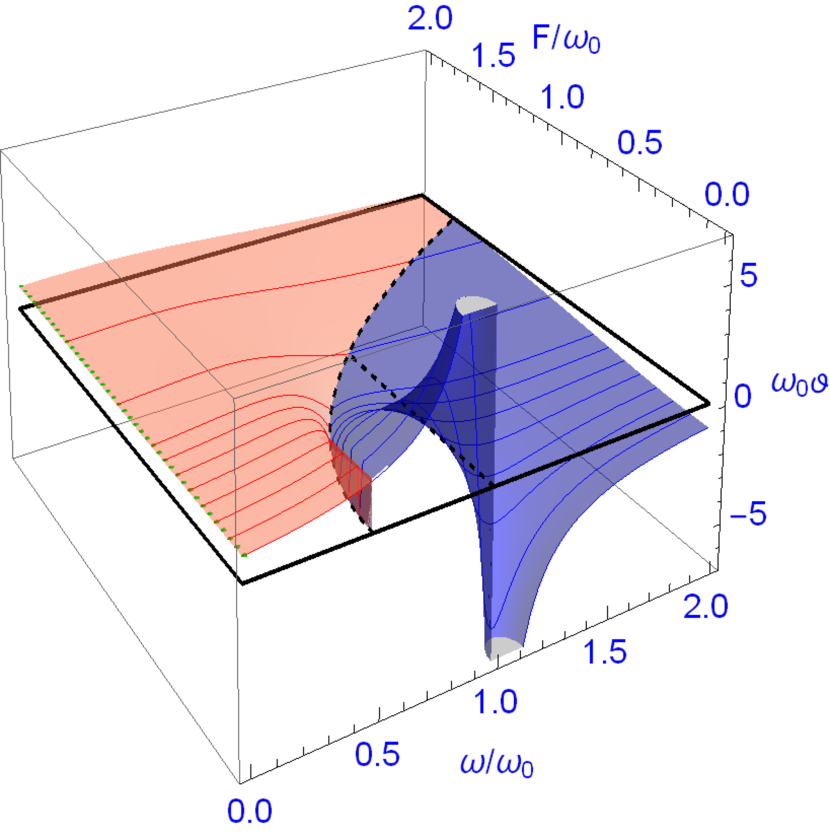
Figure 1: (Color online) Dimensionless inverse quasitemperature $\omega_{0}\vartheta$ of the spin system under the influence of a circularly polarized monochromatic driving force with amplitude $F$ and frequency $\omega$, being coupled to a harmonic-oscillator bath of inverse actual temperature $\omega_{0}\beta=1$. The blue (dark) part of the graph corresponds to the high-frequency regime $0<\Omega<\omega$, the red (gray) part to the low-frequency regime $0<\omega<\Omega$. Along the line segment $\omega=\omega_{0}$ with $F<\omega_{0}$ and along the parabola $\omega=\omega_{c}$ given by Eq. (98), both marked by black dashes, the inverse quasitemperature vanishes. A few functions $\vartheta(\omega)$ for constant $F$ are highlighted. The limit $\omega_{0}\vartheta=\omega_{0}\beta$ for $\omega/\omega_{0}\to 0$ is indicated by a green (dotted) line.

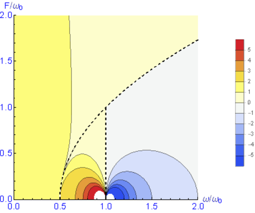
Figure 2: (Color online) Contour plot of the dimensionless inverse quasitemperature $\omega_{0}\vartheta$ with the same parameters as in Figure 1. The line segment $\omega=\omega_{0}$ with $F<\omega_{0}$ and the parabola $\omega=\omega_{c}$, where $\vartheta$ vanishes, are again marked by black dashes.

The inverse quasitemperature $\vartheta$ vanishes — meaning that the periodically driven system effectively becomes infinitely hot, so that all its Floquet states are populated equally — regardless of the bath temperature, if either $\omega=\omega_{0}$ while $0<F<\omega_{0}$, or if

$$\omega=\omega_{c}\equiv\frac{1}{2\omega_{0}}\left(F^{2}+\omega_{0}^{2}\right)\;,$$ (98)

with the latter equation defining the boundary $\omega=\Omega$ between the low- and the high-frequency regime, see Figs. 1 and 2. Along this boundary the quasienergies of all Floquet states are degenerate (modulo $\omega$), so that the appearance of infinite quasitemperature here can be understood as a resonance effect. In terms of the inverse quasitemperatures, denoted $\vartheta_{L}$ ($\vartheta_{H}$) in the low- (high-) frequency regime, there is a continuous change from $\vartheta_{L}$ to $\vartheta_{H}$, since

$$\lim_{\omega\uparrow\omega_{c}}\vartheta_{L}=\lim_{\omega\downarrow\omega_{c}}\vartheta_{H}=0\;.$$ (99)

However, the two functions $\vartheta_{L}$ and $\vartheta_{H}$ do not join smoothly at $\omega=\omega_{c}$, since their derivatives with respect to $\omega$ adopt different limits:

$$\lim_{\omega\uparrow\omega_{c}}\frac{\partial\vartheta_{L}}{\partial\omega} = -\frac{4\beta\omega_{0}^{3}\left(F^{4}+\omega_{0}^{4}\right)}{F^{4}\left(F^{2}+\omega_{0}^{2}\right)^{2}}\;,$$

$$\lim_{\omega\downarrow\omega_{c}}\frac{\partial\vartheta_{H}}{\partial\omega} = \frac{4\beta\omega_{0}^{3}\left(F-\omega_{0}\right)\left(F+\omega_{0}\right)}{F^{4}\left(F^{2}+\omega_{0}^{2}\right)}\;.$$ (100)

We will now investigate the behavior of the function $\omega_{0}\vartheta(\omega_{0}\beta,\omega/\omega_{0},F/\omega_{0})$ in the limits corresponding to the four sideways faces of the box bounding the plot displayed in Fig. 1:

(i) As already noted at the end of Sec. III.2, in the low-frequency limit $\omega/\omega_{0}\to 0$ the quasienergies (71) and (72) approach the actual energies $E_{m}=m\sqrt{\omega_{0}^{2}+F^{2}}$ (with $m=s,\ldots,-s$) of a spin exposed to a slowly varying drive. Hence, in this limit the periodic thermodynamics investigated here must reduce to the usual thermodynamics described by a canonical ensemble; in particular, the inverse quasitemperature $\vartheta$ must approach the true inverse bath temperature $\beta$. This expectation is borne out by the leading term of the low-frequency expansion

$$\omega_{0}\vartheta_{L} = \omega_{0}\beta+\frac{2\omega_{0}\beta(\omega/\omega_{0})}{(F/\omega_{0})^{2}+2}$$ (101)

$$+\frac{\omega_{0}\beta(\omega/\omega_{0})^{2}}{2\big{(}(F/\omega_{0})^{2}+2\big{)}^{2}}\left(8-4(F/\omega_{0})^{2}-\frac{(F/\omega_{0})^{4}\,\omega_{0}\beta\,\coth\left(\frac{\omega_{0}\beta}{2}\sqrt{(F/\omega_{0})^{2}+1}\right)}{\sqrt{(F/\omega_{0})^{2}+1}}\right)+O(\omega/\omega_{0})^{3}\;.$$

(ii) Next we consider the ultrahigh-frequency limit $\omega/\omega_{0}\to\infty$, keeping both $\omega_{0}\beta$ and $F/\omega_{0}$ fixed. Inspecting $q_{H}$ as defined by Eq. (89), and observing that asymptotically $\Omega=\sqrt{(\omega_{0}-\omega)^{2}+F^{2}}\sim\omega-\omega_{0}$ for $\omega/\omega_{0}\to\infty$, one finds $q_{H}\to\exp(+\beta\omega_{0})$. Recalling the reversed labeling of Floquet states for blue detuning, which accounts for the “plus” sign, this implies that in this limit the Floquet-state distribution (90) equals the Boltzmann distribution for the undriven energy eigenstates with the bath temperature. This finding can intuitively be understood as an averaging principle: In the ultrahigh-frequency limit the effect of the exernal drive on the occupation probabilities averages out, leaving one with the original thermal distribution. On the other hand, there is no such averaging principle for quasienergies; the ac Stark shift (that is, the deviation of the quasienergies from the energy eigenvalues of the undriven system) increases as $\omega$. Since our quasitemperature is defined with respect to the quasienergies, it follows that the quasitemperature has to vanish at high frequencies: By virtue of Eq. (95) one has $\vartheta_{H}\sim-\beta\omega_{0}/\omega$, and hence

$$\lim_{\omega/\omega_{0}\to\infty}\omega_{0}\vartheta_{H}\;=\;0\;;$$ (102)

as shown by Fig. 1, this limit is approached with negative quasitemperatures.

(iii) The static limit of vanishing driving amplitude, $F/\omega_{0}\to 0$, yields

$$\lim_{F/\omega_{0}\to 0}\omega_{0}\vartheta_{L}\;=\lim_{F/\omega_{0}\to 0}\omega_{0}\vartheta_{H}\;=\;\frac{\omega_{0}\beta}{1-\omega/\omega_{0}}\;,$$ (103)

easily deduced from the limits (96) in combination with the definition (95). Once again, this seemingly strange expression, exhibiting a pole at $\omega=\omega_{0}$ which is prominently visible in Fig. 1, is fully in agreement with the requirement that the periodic thermodynamics should reduce to ordinary thermodynamics when the time-periodic driving force vanishes. Namely, for $F/\omega_{0}\to 0$ the system possesses the energy eigenvalues $E_{m}=m\omega_{0}$, whereas the quasienergy representatives (71) or (72) reduce to $\varepsilon_{m}=m|\omega_{0}-\omega|$ or $\varepsilon_{m}=\omega/2+m|\omega_{0}-\omega|$ with $m=s,\ldots,-s$, while the Floquet states approach the energy eigenstates of $H_{0}=\omega_{0}S_{z}$. In this limit the parametrization of their occupation probabilities in terms of either the quasithermal distribution (91) or the standard canonical distribution must lead to identical values, implying that the usual Boltzmann factor $\exp(-\beta m\omega_{0})$ must become proportional to $\exp\left(-\vartheta m|\omega_{0}-\omega|\right)$. Hence, one has $\beta\omega_{0}=\vartheta(\omega_{0}-\omega)$ for $F/\omega_{0}\to 0$ and $0<\omega<\omega_{0}$, which immediately furnishes the above expression (103). In the case of blue detuning, for $0<\omega_{0}<\omega$, the reversed labeling of the quasienergies yields an additional “minus” sign, again leading to the limit (103).

(iv) In the converse strong-driving limit $F/\omega_{0}\to\infty$ we first focus on the regime $\omega\sim F$ where $\vartheta=\vartheta_{L}>0$. After some transformations we obtain the asymptotic form

$$\omega_{0}\vartheta_{L}\sim\omega_{0}\beta-\frac{\omega\beta}{\sqrt{(F/\omega_{0})^{2}+(\omega/\omega_{0})^{2}}}$$ (104)

in this regime, so that the inverse quasitemperature decreases monotonically with increasing driving amplitude, as exemplified by Fig. 3.

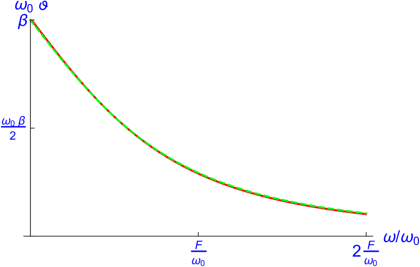
Figure 3: (Color online) Inverse dimensionless quasitemperature $\omega_{0}\vartheta$ for $\omega_{0}\beta=1$ and $F/\omega_{0}=100$ as a function of $\omega/\omega_{0}$ in the regime $0<\omega/\omega_{0}<2F/\omega_{0}$. We show the exact values of $\omega_{0}\vartheta_{L}$ (red line), as well as the asymptotic form (104) (green dashes).

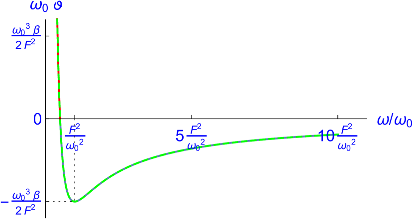
Figure 4: (Color online) Inverse dimensionless quasitemperature $\omega_{0}\vartheta$ for $\omega_{0}\beta=1$ and $F/\omega_{0}=100$ as a function of $\omega/\omega_{0}$ in the regime $\omega/\omega_{0}>(F/\omega_{0})^{2}/2$. We show the exact values of $\omega_{0}\vartheta_{L}$ (red solid line) and $\omega_{0}\vartheta_{H}$ (blue solid line), together with the asymptotic form (105) (green dashes).

In contrast, for $\omega>\omega_{c}$ as given by Eq. (98) we have $\vartheta=\vartheta_{H}<0$. Asymptotically, here we find

$$\omega_{0}\vartheta_{H}\sim-\frac{\omega_{0}\beta}{\omega/\omega_{0}}+\frac{\omega_{0}\beta}{2(\omega/\omega_{0})^{2}}\,(F/\omega_{0})^{2}\;.$$ (105)

This asymptotic function exhibits a pronounced minimum at $\omega/\omega_{0}=(F/\omega_{0})^{2}$ of depth $\omega_{0}\vartheta_{H}\sim-\omega_{0}^{3}\beta/(2F^{2})$, depicted in Fig. 4. This minimum can be understood as a result of two opposing trends: On the one hand, the averaging principle requires that the occupation probabilities approach the “undriven” Boltzmann distribution with the bath temperature for large $\omega/\omega_{0}$, which means that the inverse quasitemperature tends to a finite value proportional to $-\beta$ for large, but finite driving frequencies. On the other hand, the factor $1/\Omega$ in Eq. (95) becomes more and more predominant and forces $\vartheta$ to approach $0$ in the high-frequency regime.

V Application: Periodically driven paramagnets

V.1 Calculation of quasithermal expectation values

Starting from the proposition that the Floquet states of a periodically driven spin system be populated according to the distribution (91) we introduce the quasithermal average of the spin component in the direction of the static field,

$$\langle S_{z}\rangle_{q}\equiv\frac{1}{Z}\sum_{m=-s}^{s}\langle u_{m}(t)|S_{z}|u_{m}(t)\rangle\,\exp(-\vartheta\varepsilon_{m})\;.$$ (106)

In order to evaluate this expression we utilize the representation (70) of the Floquet functions, giving

$$Z\langle S_{z}\rangle_{q} = \sum_{m=-s}^{s}\langle m|P^{(s)\dagger}\,S_{z}\,P^{(s)}|m\rangle\,\exp(-\vartheta\varepsilon_{m})$$ (107)

$$= \mbox{Tr}\left(P^{(s)\dagger}\,S_{z}\,P^{(s)}\,\exp\!\big{(}-\vartheta G^{(s)}\big{)}\right)\;.$$

Next, we resort once more to the lifting technique: For $s=1/2$, the decomposition (60) readily yields

$$P^{\dagger}s_{z}P = \Xi^{\dagger}s_{z}\Xi$$ (108)

$$= \frac{\delta}{\Omega}\,s_{z}-\frac{\sqrt{\Omega^{2}-\delta^{2}}}{\Omega}\,s_{x}$$

by virtue of Eq. (63). Applying the irrep $r^{(s)}$, we deduce

$$P^{(s)\dagger}\,S_{z}\,P^{(s)} = r^{(s)}\big{(}P^{\dagger}s_{z}P\big{)}$$ (109)

$$= \frac{\delta}{\Omega}\,S_{z}-\frac{\sqrt{\Omega^{2}-\delta^{2}}}{\Omega}\,S_{x}\;.$$

Inserting this into the above identity (107), and calculating the trace in the eigenbasis of $S_{z}$, we obtain the important result

$$\langle S_{z}\rangle_{q}=\frac{1}{Z_{q}}\frac{\omega_{0}-\omega}{\Omega}\,\sum_{m=-s}^{s}m\,{\mathrm{e}}^{-\vartheta\Omega\,m}\;,$$ (110)

valid for both integer and half-integer $s$. In particular, this shows that the quasithermal expectation value (106) does not depend on time, despite the time-dependence of the Floquet functions. Although the unusual-looking prefactor $(\omega_{0}-\omega)/\Omega$ indeed implies that the $z$-component of the magnetization vanishes for $\omega=\omega_{0}$, it does not necessarily imply that the magnetization reverses its direction when $\omega$ is varied across $\omega_{0}$, since the reversal of the prefector’s sign can be compensated by a simultaneous change of the sign of the quasitemperature, as it happens for low driving amplitudes according to Eq. (103).

V.2 Response of paramagnetic materials to circularly polarized driving fields

As an experimentally accessible example of the above considerations, and thus as a possible laboratory application of periodic thermodynamics, we consider the magnetization of an ideal paramagnetic substance under the influence of both a static magnetic field applied in the $z$-direction, and a circularly polarized oscillating magnetic field applied in the $x$-$y$-plane. In order to facilitate comparison with the literature, here we re-install the Planck constant $\hbar$ and the Boltzmann constant $k_{\rm B}$.

We assume that the magnetic atoms of the substance have an electron shell with total angular momentum $J$, resulting from the coupling of orbital angular momentum and spin, giving the magnetic moment $\mu=g_{J}\mu_{\rm B}J$. Here $\mu_{\rm B}$ denotes the Bohr magneton, and $g_{J}$ is the Landé $g$-factor which may assume both signs; for the sake of definiteness, here we assume $g_{J}<0$. In the presence of a constant magnetic field $B_{0}$ this moment gives rise to the energy levels

$$E_{m}=-m\,g_{J}\mu_{\rm B}B_{0}\equiv m\,\hbar\omega_{0}\;,$$ (111)

where $m=-J\ldots,J$ is the magnetic quantum number. Hence, with $g_{J}<0$ the spin tends to align antiparallel to the applied magnetic field, favoring $m=-J$.

Let us briefly recall the usual textbook treatment of the ensuing thermal paramagnetism within the canonical ensemble FowlerGuggenheim39 ; Pathria11 , assuming the substance to possess a temperature $T$. Then the canonical partition function

$$Z_{0} = \sum_{m=-J}^{J}\exp\!\left(-\frac{E_{m}}{k_{\rm B}T}\right)=\sum_{m=-J}^{J}\exp\!\left({-}m\frac{\hbar\omega_{0}}{k_{B}T}\right)$$ (112)

$$= \frac{\sinh\!\left(\displaystyle\frac{2J+1}{2J}\,y_{0}\right)}{\sinh\!\left(\displaystyle\frac{y_{0}}{2J}\right)}$$

which depends on the dimensionless quantity

$$y_{0}\equiv-\frac{g_{J}\mu_{\rm B}B_{0}}{k_{\rm B}T}\,J=\frac{\hbar\omega_{0}}{k_{\rm B}T}\,J$$ (113)

serves as moment-generating function, in the sense that the thermal expectation value of the magnetization $M$ is obtained by taking the appropriate derivative of its logarithm, namely,

$$\langle M\rangle = {\frac{N}{V}\,\langle\mu\rangle}=\frac{N}{V}\,g_{J}\mu_{\rm B}\langle m\rangle$$ (114)

$$= \frac{N}{V}\frac{\partial}{\partial B_{0}}\,k_{B}T\ln Z_{0}\;.$$

Here $N/V$ denotes the density of contributing atoms. Working out this prescription, one finds the magnetization FowlerGuggenheim39 ; Pathria11

$$\langle M\rangle=M_{0}\,B_{J}(y_{0})\;,$$ (115)

where

$$M_{0}=-\frac{N}{V}\,g_{J}\mu_{\rm B}J$$ (116)

denotes the saturation magnetization, and

$$B_{J}(y)\equiv\frac{2J+1}{2J}\coth\!\left(\frac{2J+1}{2J}y\right)-\frac{1}{2J}\coth\!\left(\frac{y}{2J}\right)$$ (117)

is the so-called Brillouin function of order $J$ Brillouin27 ; this theoretical prediction (115) has been beautifully confirmed in low-temperature experiments with paramagnetic ions by Henry Henry52 already in 1952. In the weak-field limit $\mu_{\rm B}B_{0}\ll k_{\rm B}T$ one may use to approximation

$$B_{J}(y)\approx\frac{J+1}{J}\frac{y}{3}\quad\mbox{for}\quad|y|\ll 1\;,$$ (118)

giving

$$\langle M\rangle\approx\frac{N}{V}\,\frac{(g_{J}\mu_{\rm B})^{2}J(J+1)}{3k_{\rm B}T}\,B_{0}\;.$$ (119)

Returning to periodic thermodynamics, let us add the circularly polarized field $B_{1}(\cos\omega t,\sin\omega t,0)$ perpendicularly to the constant one. Then the Rabi frequency (44) can be written as

$$\Omega=\sqrt{(\omega_{0}-\omega)^{2}+(g_{J}\mu_{\rm B}B_{1}/\hbar)^{2}}\;,$$ (120)

where

$$\omega_{0}=-\frac{g_{J}\mu_{\rm B}B_{0}}{\hbar}\;$$ (121)

measures the strength of the static field in accordance with Eq. (111). Assuming that the spins’ environment is correctly described by a thermal oscillator bath with constant spectral density $J_{0}$, and the coupling to that environment is given by the expression (73), the Floquet-state occupation probabilities are governed by the distribution (91), and we can invoke the above result (110) to write the observable magnetization in the form

$$\langle M\rangle_{q} = -\frac{N}{V}\,g_{J}\mu_{\rm B}\langle S_{z}\rangle_{q}$$

$$= -\frac{N}{V}\,\frac{g_{J}\mu_{\rm B}}{Z_{q}}\,\frac{\omega_{0}-\omega}{\Omega}\sum_{m=-J}^{J}m\,\exp\!\left({-}m\frac{\hbar\Omega}{k_{\rm B}\tau}\right)\;,$$

where $\tau=1/(k_{\rm B}\vartheta)$ is the quasitemperature, and

$$Z_{q}=\sum_{m=-J}^{J}\exp\!\left({-}m\frac{\hbar\Omega}{k_{\rm B}\tau}\right)$$ (123)

is the corresponding partition function (97). Quite remarkably, this expression (V.2) is a perfect formal analog of the previous Eq. (114), since we have

$$\langle M\rangle_{q}=\frac{N}{V}\,\frac{\partial}{\partial B_{0}}\,k_{\rm B}\tau\ln Z_{q}\;,$$ (124)

taking into account the nonlinear dependence of the Rabi frequency (120) on the static field strength $B_{0}$. Hence, the resulting quasithermal magnetization can be expressed in a manner analogous to Eq. (115), namely,

$$\langle M\rangle_{q}=M_{1}\,B_{J}(y_{1})\;,$$ (125)

with modified saturation magnetization

$$M_{1}=\frac{\omega_{0}-\omega}{\Omega}\,M_{0}\;,$$ (126)

and the argument of the Brillouin function now depending on the quasitemperature,

$$y_{1}=\frac{\hbar\Omega}{k_{\rm B}\tau}\,J\;.$$ (127)

For consistency, this prediction (125) must reduce to the usual weak-field magnetiziation (119) when both $B_{1}\to 0$ and $\mu_{\rm B}B_{0}\ll k_{\rm B}T$. This is ensured by the limit (103): For sufficiently small $B_{1}$, the quasitemperature $\tau$ is related to the actual bath temperature $T$ through

$$\frac{1}{k_{\rm B}\tau}\approx\frac{\omega_{0}}{\omega_{0}-\omega}\,\frac{1}{k_{\rm B}T}\;.$$ (128)

Inserting this into Eq. (125), one can employ the approximation (118) for frequencies $\omega$ not too close to $\omega_{0}$. In this way one recovers the expected expression (119) unless $\omega\approx\omega_{0}$, in which case one has $\langle M\rangle_{q}\approx 0$.

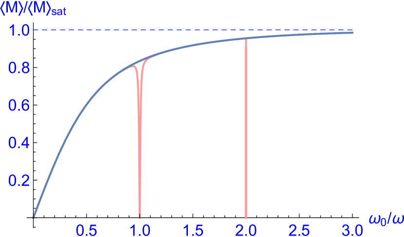
Figure 5: (Color online) Magnetizations $\langle M\rangle$ divided by their saturation magnetizations as functions of the scaled strength $\omega_{0}/\omega$ of the static field. The blue (dark) curve represents the ordinary thermal magnetization (115), the red (gray) one the quasithermal magnetization (125) for weak driving, $g_{J}\mu_{\rm B}B_{1}/(\hbar\omega)=0.01$. Here we have set $k_{\rm B}T=\hbar\omega$ and $J=7/2$.

As is evident from the above discussion, under typical conditions of electron spin resonance (ESR) with weak driving amplitudes, such that $B_{1}/B_{0}$ is on the order of $10^{-2}$ or less EatonEtAl10 , the difference between the quasithermal magnetization $\langle M\rangle_{q}$ and the customary thermal magnetization $\langle M\rangle$ is more or less negligible, except for driving frequencies close to resonance. This is illustrated in Fig. 5 for $g_{J}\mu_{\rm B}B_{1}/(\hbar\omega)=0.01$, where the bath temperature is chosen such that $k_{\rm B}T=\hbar\omega$. Here we have plotted both the usual magnetization (115) of an undriven spin system and the quasithermal magnetization (125) of its weakly driven counterpart, normalized to their respective saturation value, vs. the ratio $\omega_{0}/\omega$, representing the scaled strength $B_{0}$ of the static field. The vanishing of the quasithermal magnetization at both $\omega_{0}/\omega=1$ and $\omega_{0}/\omega=2$ clearly reflects the appearance of infinite quasitemperature at these ratios, as already observed in Fig. 1.

In marked contrast, novel types of behavior with measurable consequences occur in the regime of non-perturbatively strong driving. A particularly striking example is provided by Fig. 6, where $k_{\rm B}T=\hbar\omega_{0}$ and $J=1$: Under strong driving, the ratio $\langle M\rangle_{q}/\langle M\rangle$ actually becomes negative for frequencies $\omega_{0}<\omega<\omega_{c}$, implying that the paramagnetic material effectively becomes a diamagnetic one, reflecting the fact that under strong driving the distribution of Floquet-state occupation probabilities can differ substantially from the original thermal Boltzmann distribution. This possibility of turning a paramagnet into a diamagnet through the application of strong time-periodic forcing, as further elucidated in Fig. 7, is a “hard” prediction of periodic thermodynamics which now awaits its experimental verification.

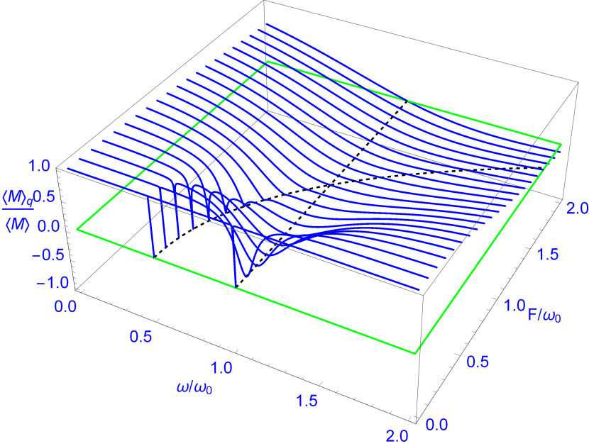
Figure 6: (Color online) Ratio $\langle M\rangle_{q}/\langle M\rangle$ of the quasithermal magnetization (125) and the customary magnetization (115) as function of $\omega/\omega_{0}$ and $F/\omega_{0}$, with $F=g_{J}\mu_{\rm B}B_{1}/\hbar$. Parameters chosen here are $k_{\rm B}T=\hbar\omega_{0}$ and $J=1$. Along the dashed black line $\omega=\omega_{0}$ and along the dashed black parabola $\omega=\omega_{c}$ given by Eq. (98) the quasithermal magnetization vanishes, so that $\langle M\rangle_{q}/\langle M\rangle$ becomes negative for strong driving with frequencies $\omega_{0}<\omega<\omega_{c}$.

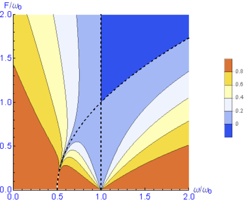
Figure 7: (Color online) Contour plot of the ratio $\langle M\rangle_{q}/\langle M\rangle$ with the same parameters as in Fig. 6. The domain in which $\langle M\rangle_{q}/\langle M\rangle$ becomes negative is indicated by the dark blue color.

VI Dissipation

Since a bath-induced transition from a Floquet state $n$ to a Floquet state $m$ is accompanied by all frequencies $\omega_{mn}^{(\ell)}$ as introduced in Eq. (9), the rate of energy dissipated in the quasistationary state is given by LangemeyerHolthaus14

$$R=-\sum_{mn\ell}\omega_{mn}^{(\ell)}\,\Gamma_{mn}^{(\ell)}\,p_{n}\;.$$ (129)

For consistency it needs to be shown that $R>0$, so that in the nonequilibrium steady state characterized by the Floquet-state distribution $\{p_{n}\}$ the energy flows from the driven system into the bath, regardless of the system’s quasitemperature DiermannEtAl19 . While this intuitive expression yields the mean dissipation rate, it is, in principle, also possible to to obtain the full probability distribution of energy exchanges between a periodically driven quantum system and a thermalized heat reservoir by applying the methods developed in Ref. GasparinettiEtAl14 .

The expression (129) can now be evaluated for all spin quantum numbers $s$. In addition to the partial transition rates (19) for neigboring Floquet states $m=n\pm 1$ listed in Secs. IV.1 and IV.2, Eq. (129) also requires the rates for pseudotransitions with $m=n$. Again dividing by $\Gamma_{0}=2\pi\gamma^{2}J_{0}$, we obtain the dimensionless diagonal transition rates

$$\Gamma_{mm}^{(\pm 1)}=\pm\frac{(2m)^{2}F^{2}}{16\left({\mathrm{e}}^{\pm\beta\omega}-1\right)\Omega^{2}}$$ (130)

for $m=s,\ldots,-s$, valid for both cases $0<\omega<\Omega$ and $0<\Omega<\omega$. In order to represent $R$ in a condensed fashion we define the polynomials

$$P_{s}(q) \equiv -2\sum_{m=0}^{2s}(m-s)^{2}q^{m}$$

$$Q_{s}(q) \equiv \frac{1}{2}\sum_{m=0}^{2s-1}(m+1)(2s-m)q^{m}$$

$$z_{s}(q) \equiv \sum_{m=0}^{2s}q^{m}\;,$$ (131)

together with the expression

$$A^{\pm}(q)\equiv\frac{\left({\mathrm{e}}^{\beta(\pm\omega+\Omega)}q-1\right)(\delta\pm\Omega)^{2}(\omega\pm\Omega)}{{\mathrm{e}}^{\beta(\pm\omega+\Omega)}-1}\;.$$ (132)

Dividing by $\omega_{0}\Gamma_{0}$, one obtains a dimensionless dissipation rate which can now be written in the form

$$R=\frac{P_{s}(q)\,\omega\,F^{2}+Q_{s}(q)\,\big{(}A^{+}(q)\mp A^{-}(q)\big{)}}{8\,z_{s}(q)\,\Omega^{2}}\;,$$ (133)

where one has to insert either $q_{L}$ or $q_{H}$ for $q$, in accordance with the case distinction (94), and the “$\mp$”-sign in the numerator becomes “minus” for $0<\omega<\Omega$, but “plus” for $0<\Omega<\omega$.

After resolving all symbols $R$ will be a function of five arguments, $R=R(s,\beta,\omega,\omega_{0},F)$, which makes the discussion more difficult than in the case of $s=1/2$ that has been considered in Ref. LangemeyerHolthaus14 . Thus, here we mention only the most perspicuous aspects of the dissipation function.

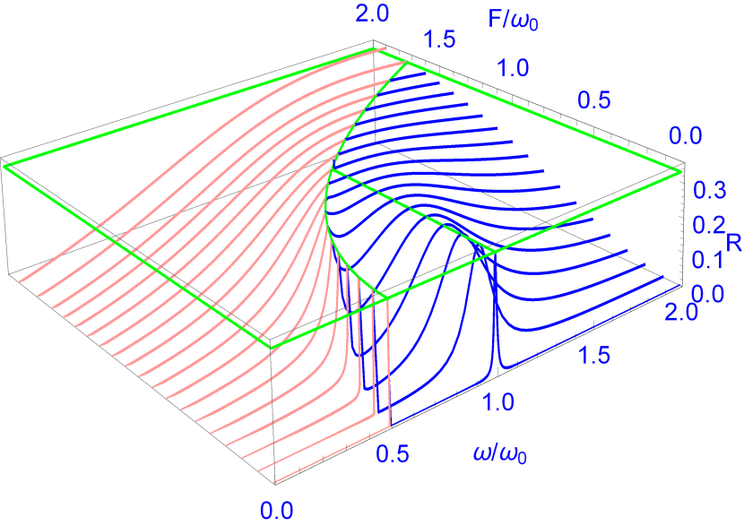
Figure 8: (Color online) The dimensionless dissipation rate $R$ for $s=1$ and $\omega_{0}\beta=1$ as a function of $\omega/\omega_{0}$ and $F/\omega_{0}$. The blue (dark) part of the graph corresponds to the high-frequency regime $0<\Omega<\omega$, the red (gray) one to the low-frequency regime $0<\omega<\Omega$. Along the line $\omega=\omega_{0}$ with $0<F<\omega_{0}$ and along the parabola $\omega=\omega_{c}$ given by Eq. (98) the dissipation rate takes on the constant value $s(s+1)/6=1/3$ (green solid lines and parabola).

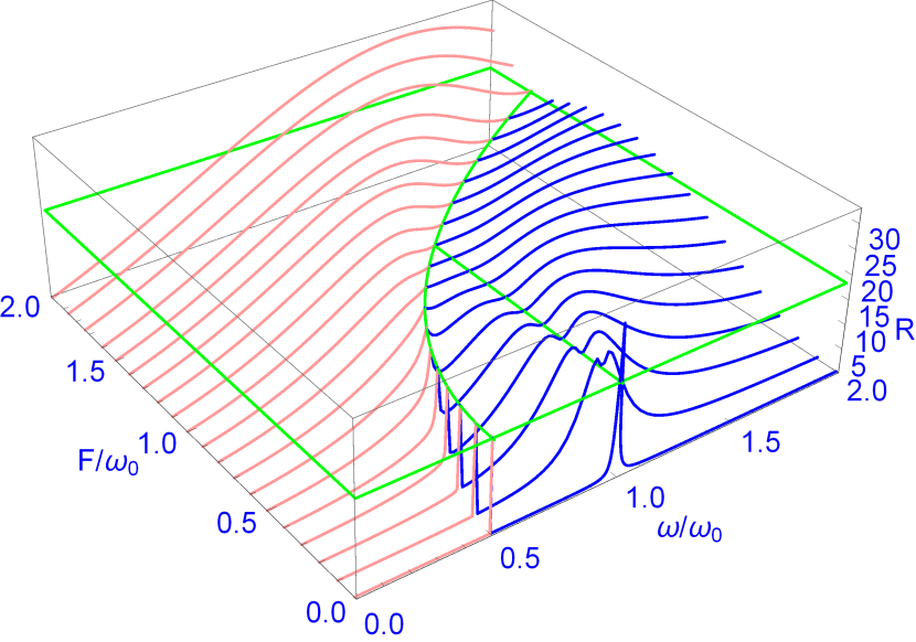
Figure 9: (Color online) As Fig. 8, but for $s=10$. Along the line $\omega=\omega_{0}$ with $0<F<\omega_{0}$ and along the parabola $\omega=\omega_{c}$ given by Eq. (98) the dissipation rate takes on the constant value $s(s+1)/6=55/3$ (green solid lines and parabola). The blue (dark) curve with $F/\omega_{0}\approx 0$ possesses two unresolved sharp maxima close to an equally sharp minimum at $\omega{\approx}\omega_{0}$.

Recall that for both $\omega=\omega_{0}$ with $0<F<\omega_{0}$ and $\omega=\omega_{c}=\left(F^{2}+\omega_{0}^{2}\right)/(2\omega_{0})$ we have $q=1$, and hence $\vartheta=0$. It turns out that along these two curves in the $(\omega,\,F)$–plane the dimensionless rate $R$ takes on the value

$$R_{0}=\frac{1}{6}s(s+1)\;,$$ (134)

as visualized in Figs. 8 and 9 for $s=1$ and $s=10$, respectively. For $1/2\leq s\leq 7/2$ this value constitutes a smooth maximum for $\omega=\omega_{0}$ and small $F/\omega_{0}$ which becomes increasingly sharp for $F/\omega_{0}\to 0$. However, for $s>7/2$ the previous maximum turns into a local minimum, the sharpness of which increases for $s\to\infty$. In contrast, along the line $\omega=\omega_{c}$ this value $R_{0}$ remains a local maximum of $R$ for all $s$, as long as $F<\omega_{0}$.

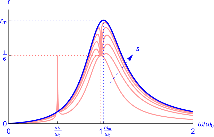
Figure 10: (Color online) The scaled dissipation rate $r=R/(s^{2}+s)$ for $s=1/2$, $5$, $10$, $20$, $50$, $200$, with bath temperature $\omega_{0}\beta=1$ and driving amplitude $F/\omega_{0}=1/4$, as a function of $\omega/\omega_{0}$. The six red (gray) curves increase with $s$ for $\omega>\omega_{c}$ as indicated by the dashed arrow. They all meet at the two points with coordinates $(\omega_{c}/\omega_{0},1/6)$ and $(1,1/6)$. The asymptotic envelope (135) is given by the blue (dark) curve, with its maximum $(\omega_{m}/\omega_{0},r_{m})$ being determined by Eqs. (136) and (137).

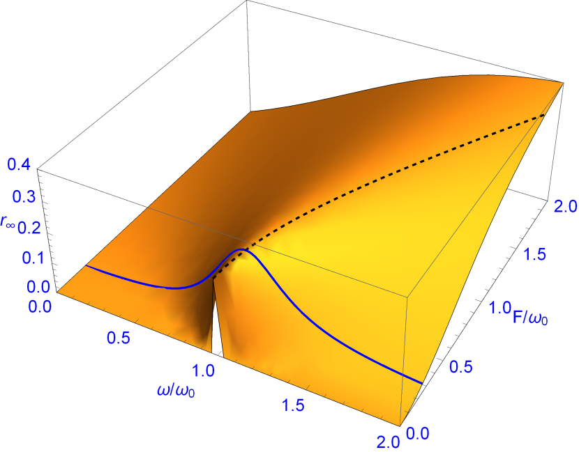
Figure 11: (Color online) The asymptotic limit $r_{\infty}(\omega/\omega_{0},F/\omega_{0})$ of the scaled dissipation rate $R/(s^{2}+s)$ for $s\to\infty$ according to Eq. (135). The particular curve with $F/\omega_{0}=1/4$ considered in Fig. 10 is shown in blue color (dark solid curve). The maximum values of the functions $r_{\infty}(\omega/\omega_{0},F/\omega_{0})$ with constant $F$ according to Eqs. (136) and (137) are indicated by a black dashed curve.

For $s\to\infty$ the scaled dissipation rate $r\equiv R/(s^{2}+s)$ tends to the limit

$$r_{\infty}(\omega/\omega_{0},F/\omega_{0})\equiv\frac{\omega}{4\omega_{0}}\,\frac{F^{2}}{F^{2}+(\omega-\omega_{0})^{2}}$$ (135)

which is independent of the heat-bath temperature. As illustrated by Fig. 10 the convergence proceeds pointwise except for $\omega=\omega_{c}$ and $\omega=\omega_{0}$ when $F<\omega_{0}$, where $r=1/6$ for all $s$. For fixed $F$ the asymptotic function $r_{\infty}(\omega/\omega_{0},F/\omega_{0})$ has a global maximum at

$$\omega_{m}/\omega_{0}=\sqrt{(F/\omega_{0})^{2}+1}\;,$$ (136)

adopting the value

$$r_{m}=\frac{1}{8}\left(1+\sqrt{(F/\omega_{0})^{2}+1}\right)\;,$$ (137)

as depicted in Figs. 10 and 11. Interestingly, the shape of $r_{\infty}$ as a function of $\omega/\omega_{0}$, indicating a resonance phenomenon leading to a maximum of the absorbed heat at $\omega=\omega_{m}$ close to $\omega_{0}$, is closely related to a prediction based on the classical Landau-Lifshitz equation Gilbert55, as sketched briefly in Appendix B.

VII Discussion

A simple harmonic oscillator which is linearly driven by an external time-periodic force while kept in contact with a thermal oscillator bath represents a nonequilibrium system, but nonetheless adopts a steady state and develops a quasistationary distribution of Floquet-state occupation probabilities which equals the Boltzmann distribution of the equilibrium model obtained in the absence of the driving force, being characterized by precisely the same temperature as that of the bath it is coupled to BreuerEtAl00 ; LangemeyerHolthaus14 .

The system considered in the present work, a spin with arbitrary spin quantum number $s$ exposed to a circularly polarized driving field while interacting with a bath of thermally occupied harmonic oscillators, may be regarded as the next basic model in a hierarchy of analytically solvable models on Periodic Thermodynamics. Exactly as in the case of the linearly forced harmonic oscillator, the system-bath interaction here induces nearest-neighbor coupling among the Floquet states of the time-periodically driven system, so that the model’s transition matrix (18) is tridiagonal, thus enforcing detailed balance. Again, the resulting quasistationary Floquet distribution turns out to be Boltzmannian, but now with a quasitemperature which differs from the physical temperature of the bath. Already the mere fact that a time-periodically driven quantum system in its steady state may exhibit a quasitemperature which is different from the actual temperature of its environment, and which can be actively controlled by adjusting, e.g., the amplitude or frequency of the driving force, in itself constitutes a noteworthy observation, suggesting that periodic thermodynamics generally may be far more subtle than usual equilibium thermodynamics based on some effective Floquet Hamiltonian.

For systems exhibiting a geometric distribution $\{p_{n}\}$ of Floquet-state occupation probabilities, the parametrization of the latter in terms of a quasitemperature is feasible if there are equidistant canonical representatives of the respective quasienergy classes DiermannEtAl19 . Therefore, we conjecture that the possibility to introduce a quasitemperature remains restricted to particularly simple integrable systems. However, the concept of quasistationary Floquet-state occupation probabilities does not require the introduction of a quasitemperature, and the exploration of the dependence of the corresponding observable quasistationary expectation values on the parameters of the driven system and its coupling to its environment constitutes a major task of periodic thermodynamics in general.

In this sense our model system is not only of basic theoretical interest, but also leads to novel predictions concerning future experiments with paramagnetic materials in strong circularly polarized fields. The very existence of a quasistationary Floquet distribution which is different from the distribution characterizing thermal equilibrium implies that the magnetic response of such a periodically driven material can be quite different from that of the undriven one; as we have demonstrated in Sec. V.2, a strong circularly polarized driving field effectively may turn a paramagnetic material into a diamagnetic one. While we are not in a position to ascertain whether the corresponding parameter regime can be reached with already existing experimental set-ups PetukhovEtAl05 , it might be worthwhile to design specifically targeted measurements for confirming this particularly striking prediction of periodic thermodynamics.

Yet, there is still more at stake here. When Brillouin published his now-famous treatise Brillouin27 on thermal paramagnetism in 1927, this was essentially a blueprint for an experimental demonstration of the quantization of angular momentum, whereas the further thermodynamical input into the theory was not to be questioned, being backed by the overwhelming generality of equilibrium thermodynamics FowlerGuggenheim39 ; Pathria11 . At the advent of periodic thermodynamics more than 90 years later, one faces an inverted situation: With the quantization of angular momentum being firmly established, it is nonequilibrium physics in the guise of periodic thermodynamics which is to be examined in measurements of paramagnetism under time-periodic driving. As has been stressed already by Kohn Kohn01 and clarified by Breuer et al. BreuerEtAl00 , quasistationary Floquet distributions are not universal, depending on the very form of the system-bath interaction. Here we have assumed an interaction of the simplistic type (11) with coupling (73) proportional to the spin operator $S_{x}$ on the system’s side and simple creation and annihilation operators (13) on the side of the bath, combined with the assumption of a constant spectral density of the bath, but there are other possibilities. Measurements of magnetism under strong driving will be sensitive to such issues; two materials which exhibit precisely the same paramagnetic response in the absence of time-periodic forcing may react differently to a static magnetic field once an additional time-periodic field has been added. Thus, despite the formal similarity of our key results (124) and (125) to their historical antecessors (114) and (115), these former equations may have the potential to open up an altogether new line of research.

Appendix A Remarks on the lifting procedure

The technique of lifting a matrix solution of the time-dependent Schrödinger equation for $s=1/2$ to general $s$, as reviewed briefly in Subsec. II.2, has been repeatedly used in this paper. In this Appendix we illustrate this technique with the help of an elementary example from classical mechanics.

Consider the motion of a rigid body, and let $\vec{r}_{0}$ denote a constant position vector in a reference frame fixedly attached to that body (“B-system”). Then this vector is expressed by

$$\vec{r}(t)=B(t)\,\vec{r}_{0}$$ (138)

with respect to some inertial laboratory system (“L-system”), where the rotational $3\times 3$-matrix $B(t)$ satisfies both $B(t)^{\top}=B(t)^{-1}$ and $\det B(t)=1$. Differentiating Eq. (138) with respect to time gives

$$\frac{{\mathrm{d}}}{{\mathrm{d}}t}\vec{r}(t)\equiv\dot{\vec{r}}=\dot{B}\,\vec{r}_{0}=\left(\dot{B}\,B^{\top}\right)\vec{r}(t)\equiv\Omega(t)\,\vec{r}(t)\;,$$ (139)

where the anti-symmetric real $3\times 3$-matrix

$$\Omega(t)=\dot{B}(t)\,B^{\top}(t)$$ (140)

has been introduced. This equation $\dot{\vec{r}}=\Omega(t)\,\vec{r}(t)$ is nothing but the matrix version of the familiar equation

$$\dot{\vec{r}}=\vec{\omega}\times\vec{r}\;,$$ (141)

involving the vector $\vec{\omega}$ of angular velocity in the L-system; this vector is constant for all points of the rigid body. Next, let $\vec{\ell}$ be the angular momentum of the rigid body in the L-system, implying that the corresponding vectors in the B-system are given by

$$\vec{\Omega} = B(t)^{\top}\,\vec{\omega}$$

$$\vec{L} = B(t)^{\top}\,\vec{\ell}\;.$$ (142)

As is well known, the linear relation between $\vec{\Omega}$ and $\vec{L}$ can be written as

$$\vec{L}=\Theta\,\vec{\Omega}\;,$$ (143)

where the time-independent, symmetric $3\times 3$-matrix $\Theta$ denotes the inertial tensor of the rigid body in the B-system. Exploiting Eqs. (142), one obtains the corresponding inertial tensor $\theta(t)$ in the L-system,

$$\vec{\ell}=B\,\vec{L}=B\,\Theta\,\vec{\Omega}=\left(B\,\Theta\,B^{\top}\right)\vec{\omega}\equiv\theta(t)\,\vec{\omega}\;.$$ (144)

Utilizing $\dot{B}B^{\top}+B{\dot{B}}^{\top}=0$ and, hence,

$${\dot{B}}^{\top}=-B^{\top}\dot{B}B^{\top}=-B^{\top}\Omega\;,$$ (145)

its time derivative takes the form

$$\dot{\theta} = \phantom{\Omega}\dot{B}\Theta B^{\top}+B\Theta\dot{B}^{\top}$$ (146)

$$= \Omega B\Theta B^{\top}+B\Theta(-B^{\top}\Omega)\;=\;\left[\Omega,\theta\right]\;,$$

with the last bracket denoting the commutator of two $3\times 3$-matrices.

While this equation (146) has been derived above in an elementary though somewhat tedious manner, we will now show that it follows directly from Eq. (140) by group-theoretical arguments.

To this end, we translate the above considerations into the appropriate group-theoretical language. Obviously, the matrices $B(t)$ connecting the B- and the L-system are elements of the Lie group $SO(3)$, and $\Omega(t)$ belongs to the associated Lie algebra $so(3)$ of real anti-symmetric $3\times 3$-matrices. Its defining equation (140) then is recognized as an immediate analog of the matrix Schrödinger equation (22) which has served as starting point in Subsec. II.2. Moreover, the transformation $\Theta\mapsto\theta=B\,\Theta\,B^{\top}$ implied by Eq. (144) can be viewed as an operation of $B$ on the space of symmetric $3\times 3$-matrices $\Theta$, and hence as a $6$-dimensional representation $R$ of $SO(3)$:

$$\theta\;=\;R(B)(\Theta)\;=\;B\,\Theta\,B^{\top}\;.$$ (147)

It is not irreducible but can be split into $1$- and $5$-dimensional irreps due to the rotational invariance of the trace of $\Theta$. The corresponding $6$-dimensional representation $r$ of the Lie algebra $so(3)$ is then given by

$$r(\Omega)(\Theta)=\left[\Omega,\Theta\right]\;.$$ (148)

This follows if $B$ is written as $B={\mathbbm{1}}+\epsilon\Omega$ with an anti-symmetric $3\times 3$-matrix $\Omega$, so that Eq. (147) yields

$$R({\mathbbm{1}}+\epsilon\Omega)(\Theta) = ({\mathbbm{1}}+\epsilon\Omega)\;\Theta\;({\mathbbm{1}}-\epsilon\Omega)$$ (149)

$$= \Theta+\epsilon\left[\Omega,\Theta\right]+O(\epsilon^{2})\;.$$

Now the definition (147) implies

$$\dot{\theta}=\left(\frac{{\mathrm{d}}}{{\mathrm{d}}t}R(B)\right)(\Theta)=\left(\frac{{\mathrm{d}}}{{\mathrm{d}}t}R(B)\right)R(B)^{-1}(\theta)\;,$$ (150)

so that the above Eq. (146) can be expressed in the form

$$\left(\frac{{\mathrm{d}}}{{\mathrm{d}}t}R(B)\right)R(B)^{-1}(\theta)=r(\Omega)(\theta)\;.$$ (151)

This is the lifted image of Eq. (140), in the same sense as the Schrödinger equation (35) in Subsec. II.2 is the lifted image of Eq. (22). Thus, it would have been possible to deduce Eq. (146) immediately from Eq. (140) in a single step.

Appendix B Damped spin precession

Instead of a driven spin coupled to a heat bath, here we consider a classical unit spin vector ${\mathbf{S}}(t)$ under the influence of both a magnetic field ${\mathbf{b}}(t)$ conforming to Eq. (41) and a nonlinear damping mechanism satisfying an equation of the Landau-Lifshitz type LL35 ,

$$\frac{{\mathrm{d}}}{{\mathrm{d}}t}{\mathbf{S}}=-{\mathbf{S}}\times{\mathbf{b}}+g\,{\mathbf{S}}\times\left({\mathbf{S}}\times{\mathbf{b}}\right)\;,$$ (152)

where the parameter $g>0$ describes the strength of the damping. (Note that the unusual signs have been chosen here because the spin vector of an electron points into the direction opposite to that of the magnetic moment.) Analogously to the elementary case of a classical damped, periodically driven oscillator it can be shown that asymptotically for $t\to\infty$ the solution of Eq. (152) becomes a rotation about the ${\mathbf{b}}_{z}$-axis with the same frequency as the field ${\mathbf{b}}(t)$ and a constant phase shift,

$${\mathbf{S}}(t)=\left(\begin{array}[]{c}\sqrt{1-z^{2}}\cos(\omega t-\phi)\\ \sqrt{1-z^{2}}\sin(\omega t-\phi)\\ z\end{array}\right)\;.$$ (153)

The functions $z=z(\omega_{0},\omega,F,g)$ and $\phi=\phi(\omega_{0},\omega,F,g)$ can be determined analytically, but are too lengthy to be reproduced here. Let

$$E(t)={\mathbf{S}}(t)\cdot{\mathbf{b}}(t)$$ (154)

be the energy of the spin in the field; this function $E(t)$ will be a periodic function of $t$ for the special solution (153). Differentiating, we find

$$\dot{E} = \dot{\mathbf{S}}\cdot{\mathbf{b}}+{\mathbf{S}}\cdot\dot{\mathbf{b}}$$ (155)

$$= -({\mathbf{S}}\times{\mathbf{b}})\cdot{\mathbf{b}}+g\big{(}{\mathbf{S}}\times({\mathbf{S}}\times{\mathbf{b}})\big{)}\cdot{\mathbf{b}}+{\mathbf{S}}\cdot\dot{\mathbf{b}}$$

$$= g\big{(}({\mathbf{S}}\cdot{\mathbf{b}})^{2}-{\mathbf{b}}^{2}\big{)}+{\mathbf{S}}\cdot\dot{\mathbf{b}}\;.$$

Integrating $\dot{E}$ over one period gives $0$, implying that the time averages of the final two terms in Eq. (155) must cancel. It is plausible to regard the first term

$$q\equiv g\big{(}({\mathbf{S}}\cdot{\mathbf{b}})^{2}-{\mathbf{b}}^{2}\big{)}\leq 0$$ (156)

as the heat loss of the driven spin due to the damping, and the second term

$$w\equiv{\mathbf{S}}\cdot\dot{\mathbf{b}}$$ (157)

as the work performed on the spin by the driving field, so that the time average of $w$ must be positive. A short calculation yields

$$w=|q|=-F\,\omega\,\sqrt{1-z^{2}}\,\sin\phi$$ (158)

which is independent of $t$, so that time-averaging is not necessary here. Note that $w\geq 0$ requires that the phase shift $\phi$ satisfies $\pi\leq\phi\leq 2\pi$. In Fig. 12 we have plotted $|q|$ as a function of $\omega/\omega_{0}$ for parameters taken from Fig. 10 and observe qualitative agreement with $r_{\infty}$ as drawn therein, suggesting a close connection between the heat-bath model and the phenomenological Landau-Lifshitz equation (152).

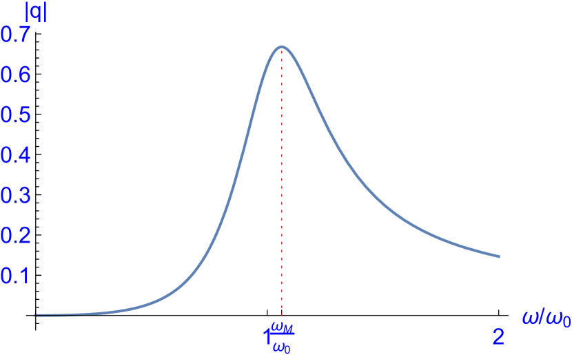
Figure 12: (Color online) Absolute value of the dissipated heat $|q|$ of the classical damped, periodically driven spin described by the Landau-Lifshitz equation (152) as a function of $\omega/\omega_{0}$. Parameters are $F/\omega_{0}=1/4$, and $g=0.1$.

A thorough investigation of this connection would require knowledge of the relation between the dissipation constant $g$ and the parameters of the heat-bath model. While a rigorous derivation of that relation is beyond the scope of this Appendix, one may obtain insight from a simple dimensional argument: Comparing the factors of dimension 1/time which set the scale for the relaxation rate implied by Eq. (152) on the one hand, and for the rates (83) and (87) on the other, we deduce

$$g|{\mathbf{b}}|\;\sim\;\Gamma_{0}=2\pi\gamma^{2}J_{0}\;,$$ (159)

where the symbol “$\sim$” is supposed to indicate “equality up to dimensionless numbers of order one”.

The rate $|q|$ of dissipated heat can then be expressed in two different ways. According to Eq. (156), one has

$$|q|\;\sim\;g|{\mathbf{b}}|^{2}\;=\;g(F^{2}+\omega_{0}^{2})\;.$$ (160)

On the other hand, the maximum dimensionless scaled dissipation rate $r_{m}$ in the classical limit $s\to\infty$ is given by Eq. (137), implying the estimate

$$R_{m} = \omega_{0}\,\Gamma_{0}\,r_{m}$$ (161)

$$\sim \Gamma_{0}\left(\omega_{0}+\sqrt{F^{2}+\omega_{0}^{2}}\right)$$

$$\sim g|{\mathbf{b}}|\left(\omega_{0}+\sqrt{F^{2}+\omega_{0}^{2}}\right)$$

$$\sim g\left(F^{2}+\omega_{0}^{2}+\omega_{0}\sqrt{F^{2}+\omega_{0}^{2}}\right)$$

for the full rate. This is compatible with the above relation (160), again hinting at an intrinsic connection between the heat-bath model studied in the main text, and the Landau-Lifshitz equation (152), so that the remarkable similarity between Figs. 10 and 12 is no coincidence.

References

- (1) Ya. B. Zel’dovich, The quasienergy of a quantum-mechanical system subjected to a periodic action, J. Exptl. Theoret. Phys. (U.S.S.R.) 51, 1492 (1966) [Sov. Phys. JETP 24, 1006 (1967)].
- (2) H. Sambe, Steady states and quasienergies of a quantum-mechanical system in an oscillating field, Phys. Rev. A 7, 2203 (1973).
- (3) A. G. Fainshtein, N. L. Manakov, and L. P. Rapoport, Some general properties of quasi-energetic spectra of quantum systems in classical monochromatic fields, J. Phys. B: Atom. Molec. Phys. 11, 2561 (1978).
- (4) R. Blümel, A. Buchleitner, R. Graham, L. Sirko, U. Smilansky, and H. Walther, Dynamical localization in the microwave interaction of Rydberg atoms: The influence of noise, Phys. Rev. A 44, 4521 (1991).
- (5) M. Grifoni and P. Hänggi, Driven quantum tunneling, Phys. Rep. 304, 229 (1998).
- (6) S. Gasparinetti, P. Solinas, S. Pugnetti, R. Fazio, and J. P. Pekola, Environment-governed dynamics in driven quantum systems, Phys. Rev. Lett. 110, 150403 (2013).
- (7) T. M. Stace, A. C. Doherty, and D. J. Reilly, Dynamical steady states in driven quantum systems, Phys. Rev. Lett. 111, 180602 (2013).
- (8) J. Zhang, P. W. Hess, A. Kyprianidis, P. Becker, A. Lee, J. Smith, G. Pagano, I.-D. Potirniche, A. C. Potter, A. Vishwanath, N. Y. Yao, and C. Monroe, Observation of a discrete time crystal, Nature 543, 217 (2017).
- (9) S. Choi, J. Choi, R. Landig, G. Kucsko, H. Zhou, J. Isoya, F. Jelezko, S. Onoda, H. Sumiya, V. Khemani, C. von Keyserlingk, N. Y. Yao, E. Demler, and M. D. Lukin, Observation of discrete time-crystalline order in a disordered dipolar many-body system, Nature 543, 221 (2017).
- (10) W. Kohn, Periodic Thermodynamics, J. Stat. Phys. 103, 417 (2001).
- (11) H.-P. Breuer, W. Huber, and F. Petruccione, Quasistationary distributions of dissipative nonlinear quantum oscillators in strong periodic driving fields, Phys. Rev. E 61, 4883 (2000).
- (12) R. Ketzmerick and W. Wustmann, Statistical mechanics of Floquet systems with regular and chaotic states, Phys. Rev. E 82, 021114 (2010).
- (13) D. W. Hone, R. Ketzmerick, and W. Kohn, Statistical mechanics of Floquet systems: The pervasive problem of near-degeneracies, Phys. Rev. E 79, 051129 (2009).
- (14) G. Bulnes Cuetara, A. Engel, and M. Esposito, Stochastic thermodynamics of rapidly driven systems, New J. Phys. 17, 055002 (2015).
- (15) T. Shirai, T. Mori, and S. Miyashita, Condition for emergence of the Floquet-Gibbs state in periodically driven open systems, Phys. Rev. E 91, 030101(R) (2015).
- (16) D. E. Liu, Classification of the Floquet statistical distribution for time-periodic open systems, Phys. Rev. B 91, 144301 (2015).
- (17) T. Iadecola, and C. Chamon, Floquet systems coupled to particle reservoirs, Phys. Rev. B 91, 184301 (2015).
- (18) T. Iadecola, T. Neupert, and C. Chamon, Occupation of topological Floquet bands in open systems, Phys. Rev. B 91, 235133 (2015).
- (19) K. I. Seetharam, C.-E. Bardyn, N. H. Lindner, M. S. Rudner, and G. Refael, Controlled population of Floquet-Bloch states via coupling to Bose and Fermi baths, Phys. Rev. X 5, 041050 (2015).
- (20) D. Vorberg, W. Wustmann, H. Schomerus, R. Ketzmerick, and A. Eckardt, Nonequilibrium steady states of ideal bosonic and fermionic quantum gases, Phys. Rev. E 92, 062119 (2015).
- (21) S. Vajna, B. Horovitz, B. Dóra, and G. Zaránd, Floquet topological phases coupled to environments and the induced photocurrent, Phys. Rev. B 94, 115145 (2016).
- (22) S. Restrepo, J. Cerrillo, V. M. Bastidas, D. G. Angelakis, and T. Brandes, Driven open quantum systems and Floquet stroboscopic dynamics, Phys. Rev. Lett. 117, 250401 (2016).
- (23) A. Lazarides and R. Moessner, Fate of a discrete time crystal in an open system, Phys. Rev. B 95, 195135 (2017).
- (24) K. I. Seetharam, C.-E. Bardyn, N. H. Lindner, M. S. Rudner, and G. Refael, Steady states of interacting Floquet insulators, Phys. Rev. B 99, 014307 (2019).
- (25) I. I. Rabi, Spin quantization in a gyrating magnetic field, Phys. Rev. 51, 652 (1937).
- (26) L. Brillouin, Les moments de rotation et le magnétisme dans la mécanique ondulatoire, J. Phys. Radium 8, 74 (1927).
- (27) W. E. Henry, Spin Paramagnetism of , , and at Liquid Helium Temperatures and in Strong Magnetic Fields, Phys. Rev. 88, 559 (1952).
- (28) R. H. Fowler and E. A. Guggenheim, Statistical Thermodynamics (Cambridge University Press, Cambridge, 1939).
- (29) For a modern exposition see, e.g., R. K. Pathria, Statistical Mechanics (Academic Press, New York; 3rd edition, 2011).
- (30) M. Langemeyer and M. Holthaus, Energy flow in periodic thermodynamics, Phys. Rev. E 89, 012101 (2014).
- (31) H.-J. Schmidt, The Floquet theory of the two-level system revisited, Z. Naturforsch. A 73, 705 (2018).
- (32) L. D. Landau and E. M. Lifshitz, Quantum Mechanics: Non-Relativistic Theory, § 57 (Butterworth-Heinemann, 3rd revised edition, reprinted 1981).
- (33) F. T. Hioe, -level quantum systems with dynamic symmetry, J. Opt. Soc. Am. B 4, 1327 (1987).
- (34) V. L. Pokrovsky and N. A. Sinitsyn, Spin transitions in time-dependent regular and random magnetic fields, Phys. Rev. B 69, 104414 (2004).
- (35) See, e.g., B. C. Hall, Lie Groups, Lie Algebras, and Representations: An Elementary Introduction, Graduate Texts in Mathematics 222 (Springer, New York; 2nd edition, 2015).
- (36) M. Holthaus and B. Just, Generalized -pulses, Phys. Rev. A 49, 1950 (1994).
- (37) J. H. Shirley, Solution of the Schrödinger equation with a Hamiltonian periodic in time, Phys. Rev. 138, B 979 (1965).
- (38) W. R. Salzman, Quantum mechanics of systems periodic in time, Phys. Rev. A 10, 461 (1974).
- (39) F. Gesztesy and H. Mitter, A note on quasi-periodic states, J. Phys. A: Math. Gen. 14, L79 (1981).
- (40) M. Holthaus, Floquet engineering with quasienergy bands of periodically driven optical lattices, J. Phys. B: At. Mol. Opt. Phys. 49, 013001 (2016).
- (41) Note a minor deviation from Ref. LangemeyerHolthaus14 , where .
- (42) O. R. Diermann, H. Frerichs, and M. Holthaus, Periodic thermodynamics of the parametrically driven harmonic oscillator, Phys. Rev. E 100, 012102 (2019).
- (43) G. R. Eaton, S. S. Eaton, D. P. Barr, and R. T. Weber, Quantitative EPR (Springer-Verlag, Wien; 2010).
- (44) S. Gasparinetti, P. Solinas, A. Braggio, and M. Sassetti, Heat-exchange statistics in driven open quantum systems, New J. Phys. 16, 115001 (2014).
- (45) L.D. Landau and E.M. Lifshitz, Theory of the dispersion of magnetic permeability in ferromagnetic bodies, Phys. Z. Sowjetunion 8, 153 (1935).
- (46) K. Petukhov, W. Wernsdorfer, A.-L. Barra, and V. Mosser, Resonant photon absorption in Fe8 single-molecule magnets detected via magnetization measurements, Phys. Rev. B 72, 052401 (2005).