Robust Reinforcement Learning in POMDPs
with Incomplete and Noisy Observations

Abstract

In real-world scenarios, the observation data for reinforcement learning with continuous control is commonly noisy and part of it may be dynamically missing over time, which violates the assumption of many current methods developed for this. We addressed the issue within the framework of partially observable Markov Decision Process (POMDP) using a model-based method, in which the transition model is estimated from the incomplete and noisy observations using a newly proposed surrogate loss function with local approximation, while the policy and value function is learned with the help of belief imputation. For the latter purpose, a generative model is constructed and is seamlessly incorporated into the belief updating procedure of POMDP, which enables robust execution even under a significant incompleteness and noise. The effectiveness of the proposed method is verified on a collection of benchmark tasks, showing that our approach outperforms several compared methods under various challenging scenarios.

1 Introduction

Significant progress has been made in reinforcement learning (RL) to solve a large number of tasks, such as Atari games (Mnih et al., 2015), board games (Silver et al., 2017b, a) and robotic control (Schulman et al., 2016). On tasks like robotic control, the agent acquires full observation through sensors from the environment to make decisions. For example, a bipedal robot perceives data through sensors such as position sensor and velocity sensor. However, in real-world scenarios, the agent could receive incomplete observation data for some reasons, namely, part of the sensor data is missing. For example, any malfunction in the sensor, too much time of preprocessing, or intrinsically, the sensors’ different sampling frequency from each other, could result in this issue (Randløv and Alstrøm, 1997). Furthermore, real-world applications usually involve noise coming from sensors, non-deterministic actions and environment (Främling, 2004). Current RL systems are not robust against these incomplete and noisy data. For example, the Proximal Policy Optimization (PPO) algorithm, involving policy network and value network, which requires complete observation to output actions, and the learning process could be damaged by the noise.

In this paper we are interested in RL method under incomplete and noisy observation. Incomplete means part of observation is dynamically missing over timestep, namely the dimension and time that observation missing occurs could not be known in advance by agent.

A passive countermeasure against the incomplete observations is to stop the executing process. However, this arrangement suffers from high cost or even is dangerous under some circumstances, e.g., for an automatic drive car driving in high speed, stopping action when data missing occurs is fatal. Another typical solution is to fill the missing components with the adjacent earlier data. However, this method is trustless especially in a rapidly changing system. A plausible method is to predict values of missing components. However, since the environments involve noise, predicting the latent state accurately is a non-trivial task.

Our work is part-in inspired by the approaches of POMDPs (Kaelbling, Littman, and Cassandra, 1998; McAllister and Rasmussen, 2017). During the execution phase of the agent, we maintain a belief state, which is the posterior distribution over latent state based on the historical incomplete and noisy observations. The belief state is employed by the policy to make decision. Our contributions are three-folds. First, we model the incomplete and noisy observations problem within the framework of POMDPs, and make several approximations to conduct a tractable and efficient belief updating. Second, we propose a new surrogate loss function with local approximation, which learns the transition model of MDP from incomplete and noisy observations. Last but not least, we propose a robust RL method with a belief imputation mechanism, which enables robust execution when the input is corrupted or partially missing. Extensive experiments on several benchmark tasks show that our approach outperforms several compared methods under various challenging scenarios.

The remainder of the paper is organized as follows. First, we give a brief outline of related work, RL and the generative model. Then we detail the new algorithm, BI-PPO, and the generative model of the incomplete and noisy observations is presented. After that, experimental results on RL benchmark tasks with incomplete and noisy observations are demonstrated. The paper concludes with conclusions and directions for future work.

2 Related Work

Concerning the methods handling missing data in RL. Randløv and Alstrøm (1997) first present a data complement method by setting up an exception network whose output is used to impute the missing values. Their method work in a MDP framework, and they impute missing data with the prediction based only on the imputed-state at last timestep. This differs from our approach, which works in a POMDP framework and employ the belief state to act based on the whole history observations and actions besides the current one.

Lizotte et al. (2008) proposed a method for batch Q-learning with missing data. They model the posterior distribution of missing data $X_{miss}$ given observed data $X_{obs}$, where $X$ is a set of trajectories. Then they sample $X^{(1)}_{miss},X^{(2)}_{miss},\ldots,X^{(N)}_{miss}$ from $X_{miss}|X_{obs}$ to construct multiple imputed datasets. The finally Q function is integrated with Q functions trained with these imputed data. Their method depends on proper assumption of the generative model and does not work well on high dimensional continuous control.

For the methods working in POMDPs, the approach of maintaining a belief state is widely used. McAllister and Rasmussen (2017) studied a special case where the partial observability has the form of additive Gaussian noise on the unobserved state. The belief is used to filter the noisy observations. Igl et al. (2018) proposed the Deep Variational RL, which directly uses a network to output distribution of the belief state from the observation, and relies on a particle filter to approximate the intractable computation of the belief updating. Their method is more like a DNN-based ’black-box’ which trying to directly output the belief state from current observation. While our method sufficiently exploits the prior knowledge of the problem structure under the incomplete and noisy observation setting by explicitly imputing the missing components from the observed part.

Many other approaches solve POMDPs by Recurrent Neural Networks (RNNs). Hausknecht and Stone (2015) proposed the Deep Recurrent Q-network (DRQN), which employ RNNs to integrate historical trajectory and is robust to partial observability on Atari games. Zhu, Li, and Poupart (2017) extended DRQN by explicitly including actions as input to the RNNs, which is called Action-specific DRQN (ADRQN). These works utilize RNNs to recurrently aggregate the history observations, while we maintain a belief state which is propagate forward by exploiting the problem structure.

3 Preliminaries

3.1 Reinforcement Learning

In RL, the decision process is modelled as a Markov Decision Process (MDP) described by the tuple $M=(\mathcal{S},\mathcal{A},{\cal T},r,\rho_{1},\gamma)$. $\mathcal{S}$, $\mathcal{A}$, ${\cal T}:\mathcal{S}\times\mathcal{A}\rightarrow\mathcal{P}(\mathcal{S})$, $r:\mathcal{S}\times{A}\rightarrow\mathbb{R}$ are the set of states, set of actions, stochastic transition function and the reward function respectively. $\rho_{1}$ is the distribution of the initial state $s_{0}$, and $\gamma\in(0,1)$ is the discount factor. Value function $V^{\pi}(s)=\mathbb{E}[R_{t}^{\gamma}|s_{t}=s]$ and action-value function $Q^{\pi}(s,a)=\mathbb{E}[R_{t}^{\gamma}|s_{t}=s,a_{t}=a]$, where $R_{t}^{\gamma}=\sum_{k=0}^{\infty}\gamma^{k}r_{t+k+1}$ , are often used in RL algorithms.

The main idea of RL methods is to update the parameter of policy $\pi_{\theta}$ towards the direction of maximizing performance objective,

$$L^{\textrm{policy}}(\theta)=\int_{\cal S\times\cal A}{{\rho^{{\pi_{\theta}}}}(s)}{\pi_{{\theta}}(a|s)r(s,a)dsda},$$

where ${\rho^{{\pi_{\theta}}}}(s)=(1-\gamma)\mathop{\sum}_{t=1}^{\infty}{\gamma^{t-1}}{\rho_{t}^{{\pi_{\theta}}}}(s)$, $\rho_{t}^{\pi_{\theta}}(s)$ is the density of $s$ at time $t$. The most commonly used gradient estimator has the form

$$\nabla_{\theta}L^{\textrm{policy}}(\theta)=\mathbb{E}_{s,a}\left[{\nabla_{\theta}\log\pi_{\theta}(a|s)A^{\pi_{\theta}}(s,a)}\right],$$

where $A^{\pi_{\theta}}(s_{t},a_{t})=Q^{\pi_{\theta}}(s_{t},a_{t})-V^{\pi_{\theta}}(s_{t})$ is the advantage function of policy $\pi_{\theta}$. The up to date algorithm to estimate $A^{\pi_{\theta}}(s_{t},a_{t})$ is the Generalized Advantage Estimator $\hat{A}^{(\gamma,\lambda)}_{t}$ (Schulman et al., 2016), which has the form

$$\hat{A}^{(\gamma,\lambda)}_{t}=\sum_{k=0}^{\infty}{(\gamma\lambda)}^{k}\left[r_{t}+\gamma\hat{V}_{\phi}(s_{t+k+1})-\hat{V}_{\phi}(s_{t+k})\right],$$

where $0<\lambda<1$ is a trade-off coefficient, and $\hat{V}_{\phi}$ is the estimated value function trained by

$${{L}^{\textrm{value}}({\phi})}=\mathbb{E}_{s_{t}}{\left\|{{V}_{\phi}}({{s}_{t}})-{{{\hat{V}}}_{t}}\right\|}^{2},$$ (1)

where $\hat{V}_{t}=\sum_{k=0}^{\infty}\gamma^{k}r_{t+k}$ is the discounted accumulated reward of from timestep $t$. PPO (Schulman et al., 2017) tactfully plug the idea of constraint on policy into the objective, by optimizing the ”surrogate” objective

$${L}^{\textrm{policy}}_{\textrm{}}({\theta})=\mathbb{E}_{s_{t},a_{t}}\left[\min\left({\omega}_{\theta}(a_{t},s_{t}){\hat{A}^{(\gamma,\lambda)}_{t}},\\ \mathop{clip}\left({\omega}_{\theta}(a_{t}|s_{t}),1-\delta,1+\delta\right){\hat{A}^{(\gamma,\lambda)}_{t}}\right)\right],$$ (2)

where ${\omega}_{\theta}(a_{t},s_{t})=\frac{{{\pi}_{\theta}}({{a}_{t}}|{{s}_{t}})}{{{\pi}_{{{\theta}_{old}}}}({{a}_{t}}|{{s}_{t}})}$, $\delta$ is the clipping parameter.

3.2 Generative Model of Incomplete and Noisy Observations

Let the state at timestep $t$ to be $s_{t}\in\mathbb{R}^{D}$, which is noisily and partially observed as $x_{t}=(s_{t}+\epsilon_{t})\odot w_{t}$, where $\epsilon_{t}\sim\mathcal{N}(0,\Sigma^{\epsilon})$, $w_{t}\in\{0,1\}^{D}$ is the observable indicator vector ($1$ for observed, $0$ for missing), and the operator $\odot$ is defined as $(s\odot w)^{(i)}\triangleq\left\{\begin{matrix}s^{(i)}&w^{(i)}=1\\ \mathsf{o}&w^{(i)}=0\end{matrix}\right.,$ where a component possesses value $\mathsf{o}$ means the data is missing; thus $x_{t}\in(\mathbb{R}\cup\{\mathsf{o}\})^{D}$.

Note that the entries of $w_{t}$ are sampled at each timestep, which make the observation dynamically missing over time. We refer missing part the ones whose values are missing, denoted as $x_{t}^{m}\in\mathbb{R}^{M_{t}}$, $M_{t}$ is the number of components of the missing part, and available part are the ones that possess values, denoted as $x_{t}^{a}\in\mathbb{R}^{D-M_{t}}$. Current RL systems could not deal with these incomplete observations directly, especially the case where the available part is dynamically changing over time.

The missing mechanism could be characterized by the conditional distribution $P(w_{t}|s_{t},x_{t},a_{t};\zeta_{t})$, where $\zeta_{t}$ denotes unknown parameter that partly determine missingness. Our method works as long as $w_{t}$ is independent of $s_{t}$. Specifically, we assume that the observation data are either Missingness Completely At Random (MCAR) or Missingness At Random (MAR) (Little and Rubin, 1987). MCAR means the missingness only depends on unknown parameters $\zeta_{t}$, while MAR is less restrictive in that the missingness could also depend on other available components, i.e.,$P(w_{t}|s_{t},x_{t},a_{t};\zeta_{t})=P(w_{t}|x_{t}^{a},a_{t};\zeta_{t})$. Since MCAR case is a particular case of MAR, we would derive our method under the MAR case throughout the paper.

4 Methods

In this section, we present the modifications on two subroutines of RL methods, which are execution and training phase respectively. During the execution phase, we conduct belief state propagation, which is employed by the policy to decide action. While in training phase, we learn the transition model of MDP, which is required by updating of the belief state and jointly trained with policy searching.

4.1 Belief State Propagation

In the execution phase, we divert the impracticable planning in original state space into belief space. In belief space, a belief state is a posterior distribution over possible original state space based on the history trajectory data, i.e., $b_{t}(s_{t})\triangleq P(s_{t}|x_{1:t},a_{1:t-1})$. The updating of belief state $b_{t}(s_{t})$ has the form by using Bayes rule,

$$b_{t}(s_{t})=\frac{P(x_{t}|s_{t},a_{t};\zeta_{t})\tilde{b}_{t}(s_{t})}{\int{P(x_{t}|s^{\prime}_{t},a_{t};\zeta_{t})\tilde{b}_{t}(s^{\prime}_{t})ds^{\prime}_{t}}},\quad\text{for }t=1,2,\ldots$$ (3)

where $$\tilde{b}_{t}(s_{t})=\int{b_{t-1}(s_{t-1}){\cal T}(s_{t}|s_{t-1},a_{t-1})ds_{t-1}}$$ (4)

$$\text{for }t=2,3,\ldots$$

where ${\cal T}$ is the transition probability function in original state space. To clarify the updating process, we introduce $\tilde{b}_{t}(s_{t})$ which is called an ”intermediate” belief state. The execution starts with a prior intermediate belief state $\tilde{b}_{1}(s_{1})$ and an initial observation $x_{1}$, the belief state $b_{t}(s_{t})$ is computed using (3), then the action $a_{t}$ is decided according to this belief state and receive an incomplete observation $x_{t+1}$, finally we yield the next belief state $b_{t+1}$ by computing (4) and (3) alternatively, and keeps iterating until end of the episode. We detail this process in the following.

First, we compute the intermediate belief state $\tilde{b}_{t}(s_{t})$ using (4) (the initial intermediate belief state $\tilde{b}_{1}$ is a parameterized distribution), which is intractable since the transition probability function ${\cal T}(s_{t}|s_{t-1},a_{t-1})$ is nonlinear. However, (4) could be approximated by replacing the nonlinear ${\cal T}(s_{t}|s_{t-1},a_{t-1})$ with first-order (linear) approximation of ${\cal T}$ w.r.t. $s_{t-1}$ at ${\mathbb{E}}_{s_{t-1}\sim b_{t-1}}[s_{t-1}]$, which reduces to $\tilde{b}_{t}(s_{t})\doteq{\cal T}(s_{t}|{\mathbb{E}}_{s_{t-1}\sim b_{t-1}}[s_{t-1}],a_{t-1})$. For tractability, we approximate the transition function by using Laplace Approximation, formulated as ${\cal T}(s_{t}|s_{t-1},a_{t-1})=\mathcal{N}\left(s_{t}|f^{\mu}(s_{t-1},a_{t-1}),f^{\Sigma}(s_{t-1},a_{t-1})\right)$, where $f^{\mu}$ and $f^{\Sigma}$ is approximated by DNNs, detailed in next section. Thus, for an intermediate state space $\tilde{b}_{t}(s_{t})$, the mean $\tilde{\mu}_{t}$ and variance $\tilde{\Sigma}_{t}$ are computed by

$$\tilde{b}_{t}(s_{t})\doteq\mathcal{N}\left(s_{t}|{\tilde{\mu}_{t}=f^{\mu}\left({\mathbb{E}}_{s_{t-1}\sim b_{t-1}}[s_{t-1}],a_{t-1}\right)},\\ {\quad\quad\quad\quad\tilde{\Sigma}_{t}=f^{\Sigma}\left({\mathbb{E}}_{s_{t-1}\sim b_{t-1}}[s_{t-1}],a_{t-1}\right)}\right)$$ (5)

Here we approximate the transition distribution as a multivariate Gaussian but focus on modeling the dynamic with a highly non-linear DNN, which helps to capture the complex dynamics of the environment. Although more general density models such as mixture of Gaussians or non-parametric models could be adopted, this could increase the difficulty of belief inference.

Then, the belief state $b_{t}$ is computed using (3). For the likelihood part $P(x_{t}|s_{t},a_{t};\zeta_{t})$, where $x_{t}\in(R\cup\{\mathsf{o}\})^{D}$ is an incomplete and noisy observation in which some components possess value $\mathsf{o}$. We denote $I^{a}_{t}=\{i|x_{t}^{(i)}\neq\mathsf{o}\}$, $I^{m}_{t}=\{i|x_{t}^{(i)}=\mathsf{o}\}$ as the available and missing indexes respectively. A sub-permutation matrix, which is used for filter and leave the available part of $x_{t}$, is constructed by ${\mathsf{H}}_{t}\in\mathbb{R}^{(D-M_{t})\times D}$ by ${\mathsf{H}}_{t}^{(j,{I_{t}^{o}}^{(j)})}=1,j=1,\ldots,D-M_{t}$ while other entries are $0$. For example, for a $D=3$ observation $x_{t}=(1,\mathsf{o},2)^{\top}$, the sub-permutation matrix is ${\mathsf{H}}_{t}=\begin{pmatrix}1&0&0\\ 0&0&1\end{pmatrix}$. Following the generative model, we have

$$P(x_{t}|s_{t},a_{t};\zeta_{t})=P(w_{t}|x_{t}^{a},a_{t};\zeta_{t})P(x_{t}^{a}|s_{t})$$ (6)

where $P(w_{t}|x_{t}^{a},a_{t};\zeta_{t})$ emerges due to the MAR assumption, $P(x_{t}^{a}|s_{t})={\cal N}({\mathsf{H}}_{t}x_{t}|{\mathsf{H}}_{t}s_{t},{\mathsf{H}}_{t}\Sigma^{\epsilon}{\mathsf{H}}_{t}^{\top})$ is marginal likelihood of the available part $x_{t}^{a}$ and has the form of linear Gaussian model (derived in Appendix LABEL:app-sec_ob_likelihood).

In addition, we adopt Gaussian as the initial intermediate belief state $\tilde{b}_{1}(s_{1})\triangleq{\cal N}(s_{1}|\tilde{\mu}_{1},\tilde{\Sigma}_{1})$. Thus by employing (3), $b_{1}(s_{1})$ is still Gaussian, and also does $\tilde{b}_{2}({s_{2}}),b_{2}(s_{2}),\ldots,\tilde{b}_{t}({s_{t}}),b_{t}(s_{t})$ by employing (5) and (3) alternatively. Specifically, given an intermediate belief state $\tilde{b}_{t}(s_{t})={\cal N}(s_{t}|\tilde{\mu}_{t},\tilde{\Sigma}_{t})$, updating of belief state $b_{t}$ in (3) is computed by

$${b}_{t}({s}_{t})=\mathcal{N}\left({s}_{t}|{{\mu}_{t}={\tilde{\mu}_{t}}+{F_{t}}\left({x_{t}-{\tilde{\mu}_{t}}}\right),}\\ {\quad\quad\quad\quad{\Sigma}_{t}={\tilde{\Sigma}_{t}}-{F_{t}}{\tilde{\Sigma}_{t}}}\right),$$ (7)

where $${F_{t}}={\tilde{\Sigma}_{t}}{\mathsf{H}}_{t}^{\top}{\left[{{{\mathsf{H}}_{t}}({\tilde{\Sigma}_{t}}+\Sigma^{\epsilon}){\mathsf{H}}_{t}^{\top}}\right]^{-1}}{{\mathsf{H}}_{t}}.$$ (8)

Note that the missing distribution $P(w_{t}|x_{t}^{a},a_{t};\zeta_{t})$ in (6) is cancelled out in (3) since it doesn’t depend on state $s_{t}$. The derivation is detailed in Appendix LABEL:app-sec_updating_belief.

In some special cases, for example, when there is no data missing occurs (but noise exists), we have ${\mathsf{H}}_{t}=I$ and Eq (8) reduces to $F_{t}={\tilde{\Sigma}_{t}}{\left[{({\tilde{\Sigma}_{t}}+\Sigma^{\epsilon})}\right]^{-1}}$. We could see that the larger the noise covariance $\Sigma^{\epsilon}$ the smaller the term $F_{t}$, which reduces the impact of current observation $x_{t}$ on the expectation $\mu_{t}$, and enlarges the uncertainty $\Sigma_{t}$ (see Eq (7)). Furthermore, when the noise is also removed (and no data missing occurs), we have $\Sigma^{\epsilon}=\mathbf{0}$ and thus $F_{t}=I$, hence $\mu_{t}$ will collapse to $x_{t}$ and $\Sigma_{t}$ to $\mathbf{0}$.

Finally, the belief state $b_{t}$ is employed by the policy $\pi$ to decide action, where we can use the exception $\mu_{t}$ of belief state for decision directly, $\pi({b}_{t})\triangleq\pi(\mu_{t}),$ or include the uncertainty term $\Sigma_{t}$ as input,

$$\pi({b}_{t})\triangleq\pi(\mu_{t},\Sigma_{t}),$$ (9)

4.2 Learning Transition Model from Incomplete and Noisy Observations

The belief state propagation in (5) requires a transition model, and the initial intermediate belief state $\tilde{b}_{1}$ also need to be learned. Some methods assume the transition model is already known (Egorov, 2015) or is approximated by a generative network, which requires a lot of data to train especially in high-dimensional tasks. However, we adopt Gaussian, which is parameterized by a highly non-linear transition network, i.e., $\hat{\mathcal{T}}(s_{t+1}|s_{t},a_{t})=\mathcal{N}\left(s_{t+1}|f^{\mu}_{\psi_{p}}(s_{t},a_{t}),f^{\Sigma}_{\psi_{p}}(s_{t},a_{t})\right)$. ${\psi_{p}}$ is parameter of the DNN, $f^{\Sigma}_{\psi_{p}}(s_{t},a_{t})$ is a state-action-dependent, positive-definite square matrix, which is parametrized by $f^{\Sigma}_{\psi_{p}}(s_{t},a_{t})=G_{\psi_{p}}(s_{t},a_{t})G_{\psi_{p}}^{\top}(s_{t},a_{t})$, where $G_{\psi_{p}}(s_{t},a_{t})$ is a lower-triangular matrix whose entries come from a linear output layer of a DNN. The initial intermediate belief state is also a Gaussian distribution $\tilde{b}_{1}(s_{1})\triangleq{\cal N}(s_{1}|\tilde{\mu}_{1},\tilde{\Sigma}_{1})$. For simplification, we denote $\psi\triangleq(\psi_{p},\tilde{\mu}_{1},\tilde{\Sigma}_{1})$. The log-likelihood of observations given actions, i.e., $\log P(x_{1:T}|a_{1:T};\psi)$, is

$$\begin{multlined}{L}(\psi)=\log\int{\tilde{b}(s_{1};\psi)P(x_{1}|s_{1},a_{1};\zeta_{1})\cdot}\\ {\prod_{t=1}^{T-1}\hat{\mathcal{T}}(s_{t+1}|s_{t},a_{t};\psi)P(x_{t+1}|s_{t+1},a_{t+1};\zeta_{t+1})ds_{1:T}}\end{multlined}{L}(\psi)=\log\int{\tilde{b}(s_{1};\psi)P(x_{1}|s_{1},a_{1};\zeta_{1})\cdot}\\ {\prod_{t=1}^{T-1}\hat{\mathcal{T}}(s_{t+1}|s_{t},a_{t};\psi)P(x_{t+1}|s_{t+1},a_{t+1};\zeta_{t+1})ds_{1:T}}$$ (10)

Note that the unknown parameter $\zeta_{t}$ (which partly determines the missing vector) doesn’t need to be learned (is not employed by belief updating) and doesn’t influence the learning of other parameters since it is independent of $s_{t}$ (see Eq (6)). The multiple production in (10) makes the objective difficult to optimize directly. Instead, we introduce the following local approximation,

$${\hat{L}_{\psi^{\prime}}}(\psi)=\log\int{\tilde{b}_{1}(s_{1};\psi)P(x_{1}|s_{1},a_{1};\zeta_{1})ds_{1}}\\ +\sum_{t=1}^{T-1}\left[\log\int{b_{t}(s_{t};\psi^{\prime})\hat{\cal T}(s_{t+1}|s_{t},a_{t};{\psi})\cdot}\\ {\quad\quad\quad P(x_{t+1}|s_{t+1},a_{t+1};\zeta_{t+1})ds_{t}ds_{t+1}}\right],$$ (11)

where $\psi^{\prime}$ is a value of variable $\psi$.

Due to the intractable nonlinear $\hat{\cal T}$, Eq (11) is approximated by replacing the nonlinear $g(s_{t},x_{t+1},a_{t})=\int{\hat{\cal T}(s_{t+1}|s_{t},a_{t};{\psi})P(x_{t+1}|s_{t+1})ds_{t+1}}$ with first-order (linear) approximation w.r.t. $s_{t}$ at ${\mathbb{E}}_{s_{t}\sim b_{t}(s_{t};{\psi^{\prime}})}[s_{t}]=\mu_{t}$. Thus the final objective function has the form

$${\hat{L}}^{\textrm{model}}_{\psi^{\prime}}(\psi)=\log{\cal N}\left({\mathsf{H}}_{1}x_{1}|{\mathsf{H}}_{1}\tilde{\mu}_{1},{\mathsf{H}}_{1}\left(\tilde{\Sigma}_{1}+\Sigma^{\epsilon}\right){\mathsf{H}}_{1}^{\top}\right)\\ +\sum_{t=1}^{T-1}\left[\log\mathcal{N}\left({\mathsf{H}}_{t+1}x_{t+1}|{\mathsf{H}}_{t+1}f^{\mu}_{\psi_{p}}(\mu_{t},a_{t}),\\ {{\mathsf{H}}_{t+1}\left(f^{\Sigma}_{\psi_{p}}(\mu_{t},a_{t})+\Sigma^{\epsilon}\right){\mathsf{H}}_{t+1}^{\top}}\right)\right]$$ (12)

The parameters of the noise model could be learned in principle, e.g., by imposing extra regularization terms (e.g., low-rank constraints, $l_{2}$-norm) over the parameters.

4.3 Jointly Learning with Policy Searching

We extend PPO from MDPs to a special-case of POMDPs (where the observations are incomplete and noisy), which we call Belief Imputation PPO (BI-PPO). The input to the policy and value network of PPO is modified to be belief state, i.e., $(\mu_{t},\Sigma_{t})$, as Eq (9) shows. Whereas we only implement our method by extending PPO, it could also be generally extended to other DNN-based RL algorithms. We integrate the objectives by minimizing the following objective function,

$$J(\theta,\phi,\psi)=-{{L}^{\textrm{policy}}_{\textrm{}}({\theta})}+\lambda_{v}{{L}^{\textrm{value}}({\phi})}-\lambda_{p}{{\hat{L}}^{\textrm{model}}_{\psi^{\prime}}({\psi})}$$ (13)

where $\lambda_{v}$ and $\lambda_{p}$ are the coefficients. The transition network shares parameter with the policy and value networks, and these three networks are trained jointly. This architecture could assist in learning a more robust representation and promote the performance of RL, as we will evaluate in experiments. Since we adopt the normalized advantage values and rewards to train policy and value network, all the three terms have the same magnitude across different tasks (the term ${{\hat{L}}^{\textrm{model}}_{\psi^{\prime}}({\psi})}$ could be seen as a likelihood term). Thus we could use the same setting of the hyper-parameters across different tasks in principle.The BI-PPO algorithm is presented in Algorithm 1.

Algorithm 1 BI-PPO

1:  for $i=1$ to TIMESTEPS_MAX$/T$ do

2:     // Execution Phase

3:     Receive observation $x_{1}$ from environment

4:     Start with $\tilde{b}_{1}=\mathcal{N}(\tilde{\mu}_{1},\tilde{\Sigma}_{1})$

5:     for $t=1$ to $T$ do

6:        Update the belief state $b_{t}=\mathcal{N}(\mu_{t},\Sigma_{t})$ by (7)

7:        Perform $a_{t}$ according to $\pi(b_{t})$ by (9)

8:        Receive reward $r_{t}$ and incomplete observation $x_{t+1}$

9:        Update the intermediate belief state $\tilde{b}_{t+1}$ by (5)

10:     end for

11:     // Training Phase

12:     for $k=1$ to Epoches_Max do

13:        Compute advantage $\hat{A}_{t}^{(\lambda,\gamma)}$, for $t=1,\ldots,T$

14:        for $t=1$ to $T$ do

15:           Update belief state $b_{t}=\mathcal{N}(\mu_{t},\Sigma_{t})$ by (7) with $\tilde{b}_{t}$ and $x_{t}$

16:           Train networks with the tuple $(\mu_{t},\Sigma_{t},a_{t},A_{t}^{(\lambda,\gamma)},x_{t+1})$ by (13)

17:           Update the intermediate belief state $\tilde{b}_{t+1}$ by (5)

18:        end for

19:     end for

20:  end for

5 Experiments

5.1 Experiments Setting

We designed our experiments to investigate the following questions:

1. Could BI-PPO be robust to the incomplete and noisy observations issue for control tasks? To what extent of missing and noise could it be robust?

2. Could BI-PPO contribute to learning regarding episode rewards and data efficiency?

To answer 1, we evaluate BI-PPO under different missing and noise settings on benchmark continuous control tasks. Specially, each component of observation has a probability of rate to be missing and is contaminated with additive Gaussian noise. Concerning 2, we compare BI-PPO with several prior policy optimization algorithms, regarding episode rewards and the required timestep to hit a threshold. The following two sections discuss these two questions respectively.

Simulated Tasks. We evaluated our methods on 8 benchmarks simulated locomotion tasks, which is implemented in OpenAI Gym v0.9.3. (Brockman et al., 2016) using the MuJoCo (Todorov, Erez, and Tassa, 2012) physics engine. The 8 benchmark tasks are HalfCheetah, Hopper, Walker2d, Ant, Swimmer, Reacher, InvertedDoublePendulum, InvertedPendulum respectively.

Implementation Details. We implemented our algorithms based on the implementations of PPO (Dhariwal et al., 2017). Similarly in Schulman et al. (2017), we used discount factor $\gamma=0.99$, GAE parameter $\lambda=0.95$, PPO clipping parameter is setting to be $0.2$, and Adam is used to for learning the weights of deep networks with a base learning rate of $lr=3\times 10^{-4}$, Adam epsilon $\epsilon_{adam}=1\times 10^{-5}$. Empirically, we set the penalty coefficient $\lambda_{v}=1.0,\lambda_{p}=1.0$. All three DNNs has two hidden layers of 64 units each and shares the first layer.

5.2 Evaluation with Incomplete and Noisy Observations

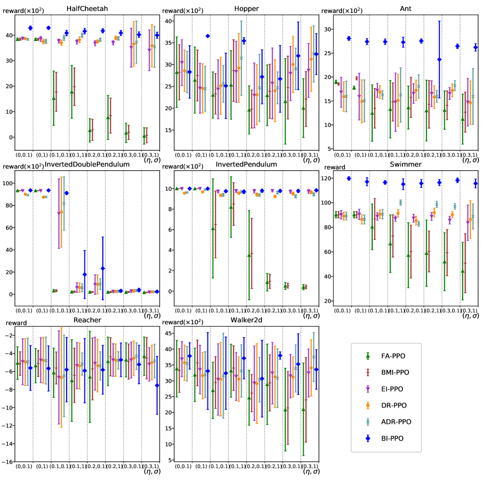
Figure 1: Episode rewards under different missing ratio $\eta$ and noise factor $\sigma$ settings on benchmark tasks. The error bars show $\pm 1$ standard deviation of the mean reward given 10 episodes of the trained model. The horizontal axis shows different combination of missing ratio $\eta$ and noise level $\sigma$, while the vertical axis shows the rewards. The rewards of different methods are shown for each setting.

Table 1: Results of maximum attained episode rewards and timesteps to hit a threshold within 2 million timesteps, averaged over 3 random seeds. (a) shows the maximum attained episode reward. (b) shows the timesteps to hit a prescribed threshold. The thresholds for all environment were chosen according to Wu et al. (2017) except Ant and HalfCheetah since we evaluate algorithms within 1/15 of their limiting timesteps.

	(a) Maximum Rewards				(b) Timesteps ($\times 10^{3}$) to hit threshold
	BI-PPO	EI-PPO	PPO	ACKTR	Threshold	BI-PPO	EI-PPO	PPO	ACKTR
HalfCheetah	4156	3735	1549	3233	2100	235	425	$\infty$	850
Hopper	3828	3595	3622	3309	2000	184	231	209	502
Ant	2988	1628	2448	3566	2500	1220	$\infty$	$\infty$	825
Inverted DoublePendulum	9345	9342	9333	9342	9100	104	137	155	348
InvertedPendulum	1000	1000	1000	1000	950	18	22	18	110
Swimmer	115	105	118	47	90	493	1073	550	$\infty$
Reacher	-5	-4	-1	-3	-7	176	268	137	250
Walker2d	4352	4034	4285	2398	3000	489	456	252	$\infty$

To investigate robustness against incomplete and noisy observations, we investigate methods under different missing ratio and noise level. For missing mechanism, we design for the MAR case, the probability function of $i$-th observable indicator ($i=1,\dots,D$) is

$$P(w^{(i)}_{t}=1|x_{t}^{a},a_{t};\zeta_{t})\triangleq P(w^{(i)}_{t}=1|x_{t}^{a},a_{t},\zeta)P(w^{(i)}_{t}=1|\zeta)$$

The two terms in RHS represent the missing conditioned on observed and unknown variables, jointly impact $w_{t}^{(i)}$. Only both two distributions output $1$ could component $i$ be observable. They have forms

$$\begin{gathered}\begin{multlined}P(w^{(i)}_{t}{=}1|x_{t}^{a},a_{t},\zeta)\triangleq 1-{min\left({g}({x_{t}^{a}}^{\top}\beta_{1,i}+a_{t}^{\top}\beta_{2,i}+\beta_{3,i}),\zeta\right)}\end{multlined}P(w^{(i)}_{t}{=}1|x_{t}^{a},a_{t},\zeta)\triangleq 1-{min\left({g}({x_{t}^{a}}^{\top}\beta_{1,i}+a_{t}^{\top}\beta_{2,i}+\beta_{3,i}),\zeta\right)}\\ P(w^{(i)}_{t}=1|\zeta)\triangleq 1-\zeta,\end{gathered}$$

where $g$ is the sigmoid function, $\beta_{1,i}$, $\beta_{2,i}$, $\beta_{3,i}$ are random variable sampled from Gaussian distribution, $0<\zeta<1$ is the parameter of Bernoulli distribution. We use $\min$ operation to manually control the missing level in our experiments. To explicitly compare the result under different missing level, we refer $\eta=\max_{x_{t}^{a},a_{t}}P(w^{(i)}_{t}=0|x_{t}^{a},a_{t};\zeta_{t})$ to the missing ratio, and we set $\eta=0,0.1,0.2,0.3$ for different settings by tuning $\zeta$. The noise levels are controlled by a noise factor $\sigma=0.1,1$, such that the noises are $\sqrt{\Sigma^{\epsilon}}=\sigma\times 0.01\times I$. We run each trial for $2\times 10^{6}$ timesteps (except for RNN-based comparison methods, which require more timesteps and is trained with $2\times 10^{7}$ timesteps) and save the trained model every 2048 timesteps, then the model which achieves the best performance during the training process is employed to execute for 10 episodes. We measure the episode rewards, imputed state precision and execution time of each method.

We compare our method against the following algorithms. 1) The naive Fill Adjacent (FA) method is baseline, where the missing value is imputed with adjacent earlier value. 2) Bayesian Multiple Imputation (BMI) method (Lizotte et al., 2008), which imputes missing values with posterior of observed data to build policies. 3) Exception Imputation (EI) (Randløv and Alstrøm, 1997), which complement the missing values with a predictive state directly. 4) Deep Recurrent Q-network (DRQN) (Hausknecht and Stone, 2015), which add recurrent LSTM architecture to the networks. 5) Action-specific DRQN (ADRQN) (Zhu, Li, and Poupart, 2017), which extra including the action as input of RNNs. We implement these methods using PPO, thus are called FA-PPO, BMI-PPO, EI-PPO, DR-PPO, ADR-PPO respectively.

Episode Rewards: Fig. 1 shows episode rewards results under different missing ratio and noise level on benchmark tasks. At low noise without missing, all methods work relatively well. However, as missing ratio increase, FA-PPO works poorly, while BMI-PPO works slightly better than FA-PPO but a lot worse than BI-PPO. DR-PPO, ADR-PPO performs better than EI-PPO, but much worse than BI-PPO. This is partly due to the reason that the hidden representation yielded by a RNN network is not stable when the input contains corrupted or missing values. BI-PPO outperform EI-PPO by a large margin, especially on HalfCheetah, Ant, Swimmer, Walker2d. All methods don’t work well on InvertedDoublePendulum with high missing ratio. We speculate that the state in this task is compact and all components have critical information for decision. Nevertheless, overall BI-PPO shows robustness against significant incompleteness and noise, and work pretty well especially on high dimensional tasks like HalfCheetah, Hopper, and Ant.

Imputed State Precision: The imputed state precision could partly reflect why the algorithms perform in the level. We measure MSE between the imputed state and the latent system state, which could be obtained in the simulator. The imputed state precision results are almost consistent with rewards results in Fig. 1, and are provided in Appendix LABEL:app-sec_observation_precision.

Execution Time Complexity: We report model run time for EI-PPO, DR-PPO, ADR-PPO and BI-PPO. The former three ones run for average $2.7$s in an episode over all tasks, with constant time complexity w.r.t. the number of timetsteps $T$. While BI-PPO runs for average $5.1$s and scales with $\mathcal{O}\left(T(D(1-\eta))^{3}\right)$ time complexity.

5.3 Evaluation with Complete and Clean Observations

In this section, we investigate whether BI-PPO could assist in learning better policy, regarding rewards and sample efficiency. Thus we evaluate them with complete and clean observations. We compared BI-PPO and EI-PPO against the following methods: the original PPO (Schulman et al., 2017), Actor Critic using Kronecker-Factored Trust Region (ACKTR) (Wu et al., 2017). Both of BI-PPO and EI-PPO set up an additional transition network, but approximate the transition model in a different way. We use OpenAI Baselines (Dhariwal et al., 2017) implementations of these algorithms. Each algorithm runs for $2$ million timesteps, and is averaged over the 3 random seeds.

Maximum Episode Rewards: Table 1 (a) shows maximum episode rewards within 2 million timesteps. Table 1 (a) shows that both BI-PPO and EI-PPO significantly outperform the original PPO. Especially on HalfCheetah and Ant, BI-PPO achieves $268\%$ and $120\%$ of the original PPO maximum reward. This shows that our approach of jointly learning the required model for computing the belief state with the policy is beneficial to improve the overall generalization capability of the system. On HalfCheetah, Hopper, InvertedDoublePendulum, and Walker2d, BI-PPO performs better than ACKTR. BI-PPO outperform EI-PPO on almost all tasks except Reacher, which shows that the probabilistic approximation to transition function is necessary.

Sample Efficiency: Table 1 (b) shows the timesteps required by algorithms to hit a prescribed threshold within $2$ million timesteps. The thresholds for all environments were chosen according to Wu et al. (2017) except Ant and HalfCheetah since we evaluate algorithms within 1/15 of their timesteps. Table 1 (b) shows that BI-PPO significantly outperform ACKTR on HalfCheetah, Hopper, InvertedDoublePendulum, Reacher. We could also observe that BI-PPO requires fewer timesteps than EI-PPO and the original PPO on almost all tasks except Swimmer and Reacher.

6 Conclusions

In this paper, we propose a new algorithm, BI-PPO, addressing the incomplete and noisy observations problem for continuous control using a model-based method, in which the transition model is estimated from the incomplete and noisy observations using a newly proposed surrogate loss function with local approximation. To implement belief imputation for execution and training, we construct a generative model and seamlessly incorporate it into the belief updating procedure of POMDP. Furthermore, we propose a robust RL method with belief imputation, which enables robust execution even under a significant incompleteness and noise. Experiments verify the effectiveness of the proposed method, showing that our approach outperforms several compared methods under various challenging scenarios. Besides, BI-PPO could also improve the original PPO by a large margin regarding rewards and data efficiency, and is competitive with the state-of-the-art policy gradient methods.

As part of our future work, we plan to handle a slightly different but more difficult case where some sensors suddenly produce totally different values. An approach to handle this case, based on this work, is to treat such values as outliers, and weight down their influence on the belief imputation or just throw them away.

appendix.pdf,-

References

- Brockman et al. (2016) Brockman, G.; Cheung, V.; Pettersson, L.; Schneider, J.; Schulman, J.; Tang, J.; and Zaremba, W. 2016. Openai gym.
- Dhariwal et al. (2017) Dhariwal, P.; Hesse, C.; Klimov, O.; Nichol, A.; Plappert, M.; Radford, A.; Schulman, J.; Sidor, S.; and Wu, Y. 2017. Openai baselines. https://github.com/openai/baselines.
- Egorov (2015) Egorov, M. 2015. Deep reinforcement learning with pomdps.
- Främling (2004) Främling, K. 2004. Reinforcement learning in a noisy environment: light-seeking robot. WSEAS Transactions on Systems 3(2):714–719.
- Hausknecht and Stone (2015) Hausknecht, M. J., and Stone, P. 2015. Deep recurrent q-learning for partially observable mdps. arXiv preprint arXiv:1507.06527.
- Igl et al. (2018) Igl, M.; Zintgraf, L. M.; Le, T. A.; Wood, F.; and Whiteson, S. 2018. Deep variational reinforcement learning for pomdps. international conference on machine learning 2122–2131.
- Kaelbling, Littman, and Cassandra (1998) Kaelbling, L. P.; Littman, M. L.; and Cassandra, A. R. 1998. Planning and acting in partially observable stochastic domains. Artificial Intelligence 101(1):99–134.
- Little and Rubin (1987) Little, R. J. A., and Rubin, D. B. 1987. Statistical analysis with missing data.
- Lizotte et al. (2008) Lizotte, D. J.; Gunter, L.; Laber, E. B.; and Murphy, S. A. 2008. Missing Data and Uncertainty in Batch Reinforcement Learning. NIPS-08 Workshop on Model Uncertainty and Risk in Reinforcement Learning 1–8.
- McAllister and Rasmussen (2017) McAllister, R., and Rasmussen, C. E. 2017. Data-efficient reinforcement learning in continuous state-action gaussian-pomdps. In NIPS 2017, 2040–2049.
- Mnih et al. (2015) Mnih, V.; Kavukcuoglu, K.; Silver, D.; Rusu, A. A.; Veness, J.; Bellemare, M. G.; Graves, A.; Riedmiller, M.; Fidjeland, A. K.; Ostrovski, G.; et al. 2015. Human-level control through deep reinforcement learning. Nature 518(7540):529.
- Randløv and Alstrøm (1997) Randløv, J., and Alstrøm, P. 1997. Reinforcement learning based on incomplete state data.
- Schulman et al. (2016) Schulman, J.; Moritz, P.; Levine, S.; Jordan, M. I.; and Abbeel, P. 2016. High-dimensional continuous control using generalized advantage estimation. international conference on learning representations.
- Schulman et al. (2017) Schulman, J.; Wolski, F.; Dhariwal, P.; Radford, A.; and Klimov, O. 2017. Proximal policy optimization algorithms. arXiv preprint arXiv:1707.06347.
- Silver et al. (2017a) Silver, D.; Hubert, T.; Schrittwieser, J.; Antonoglou, I.; Lai, M.; Guez, A.; Lanctot, M.; Sifre, L.; Kumaran, D.; Graepel, T.; et al. 2017a. Mastering chess and shogi by self-play with a general reinforcement learning algorithm. arXiv preprint arXiv:1712.01815.
- Silver et al. (2017b) Silver, D.; Schrittwieser, J.; Simonyan, K.; Antonoglou, I.; Huang, A.; Guez, A.; Hubert, T.; Baker, L.; Lai, M.; Bolton, A.; et al. 2017b. Mastering the game of go without human knowledge. Nature 550(7676):354.
- Todorov, Erez, and Tassa (2012) Todorov, E.; Erez, T.; and Tassa, Y. 2012. Mujoco: A physics engine for model-based control. In Ieee/rsj International Conference on Intelligent Robots and Systems, 5026–5033.
- Wu et al. (2017) Wu, Y.; Mansimov, E.; Grosse, R. B.; Liao, S.; and Ba, J. 2017. Scalable trust-region method for deep reinforcement learning using kronecker-factored approximation. neural information processing systems 5279–5288.
- Zhu, Li, and Poupart (2017) Zhu, P.; Li, X.; and Poupart, P. 2017. On improving deep reinforcement learning for pomdps. arXiv preprint arXiv:1804.06309.