Limits of sequences of pseudo-Anosov maps and of hyperbolic 3-manifolds

Abstract.

There are two objects naturally associated with a braid $\beta\in B_{n}$ of pseudo-Anosov type: a (relative) pseudo-Anosov homeomorphism $\varphi_{\beta}\colon S^{2}\to S^{2}$; and the finite volume complete hyperbolic structure on the 3-manifold $M_{\beta}$ obtained by excising the braid closure of $\beta$, together with its braid axis, from $S^{3}$. We show the disconnect between these objects, by exhibiting a family of braids $\{\beta_{q}:q\in{{\mathbb{Q}}}\cap(0,1/3]\}$ with the properties that: on the one hand, there is a fixed homeomorphism $\varphi_{0}\colon S^{2}\to S^{2}$ to which the (suitably normalized) homeomorphisms $\varphi_{\beta_{q}}$ converge as $q\to 0$; while on the other hand, there are infinitely many distinct hyperbolic 3-manifolds which arise as geometric limits of the form $\lim_{k\to\infty}M_{\beta_{q_{k}}}$, for sequences $q_{k}\to 0$.

1. Introduction

This article presents a somewhat surprising phenomenon on the interface between the theories of surface homeomorphisms and of 3-manifold geometry. Two theorems due to Thurston associate to certain mapping classes on a surface — the pseudo-Anosov mapping classes — two different types of canonical objects.

• The Classification Theorem for Surface Homeomorphisms [26, 13, 7] states that every irreducible mapping class which is not of finite order contains a pseudo-Anosov homeomorphism, which is unique up to topological conjugacy. Such a mapping class is said to be of pseudo-Anosov type.

• The Hyperbolization Theorem for Fibered 3-Manifolds [27, 22, 20] states that the mapping torus of a mapping class admits a complete hyperbolic metric of finite volume (unique up to isometry by the Mostow-Prasad Theorem) if and only if the mapping class is of pseudo-Anosov type.

In this paper we consider mapping classes of marked spheres, represented by elements of Artin’s braid groups: an $n$-braid $\beta\in B_{n}$ defines a mapping class on the $n$-marked disk, and hence on the $(n+1)$-marked sphere. We say that $\beta$ is of pseudo-Anosov type if and only if the corresponding mapping class is, and in this case we can associate to it:

• a homeomorphism $\varphi_{\beta}\colon S^{2}\to S^{2}$, unique up to conjugacy, which is pseudo-Anosov relative to the marked points (that is, whose invariant foliations are permitted to have $1$-pronged singularities at these points); and

• the hyperbolic $3$-manifold $M_{\beta}=S^{3}\setminus({\overline{\beta}}\cup A)$ — where ${\overline{\beta}}$ is the closure of $\beta$ and $A$ is its braid axis — which is homeomorphic to the mapping torus of $\varphi_{\beta}$ (acting on the sphere punctured at the $n+1$ marked points).

We will present a family of pseudo-Anosov braids $\{\beta_{q}:q\in{{\mathbb{Q}}}\cap(0,1/3]\}$, with $\beta_{m/n}\in B_{n+2}$, with the following properties:

• The pseudo-Anosov homeomorphisms $\varphi_{q}:=\varphi_{\beta_{q}}:S^{2}\to S^{2}$ can be normalized in such a way that $\varphi_{q}\to\varphi_{0}$ as $q\to 0$, where $\varphi_{0}$ is a fixed sphere homeomorphism (the tight horseshoe map, derived from Smale’s horseshoe map).

• The hyperbolic $3$-manifolds $M_{q}:=M_{\beta_{q}}$ have the property that there are infinitely many distinct finite volume hyperbolic $3$-manifolds which can be obtained as geometric limits $\lim_{k\to\infty}M_{q_{k}}$ for some sequence $q_{k}\to 0$.

The braids $\beta_{q}$ are the NBT braids of [17]: they are pseudo-Anosov braids for which the corresponding pseudo-Anosov homeomorphisms $\varphi_{q}$ have particularly simple train tracks (see Remark 5). The fact that $\varphi_{q}\to\varphi_{0}$ as $q\to 0$ is a straightforward consequence of results of [6]: the main content of this paper is an analysis of possible geometric limits of sequences $M_{q_{k}}$.

It is interesting to contrast this work with the surprising discovery due to Farb, Leininger, and Margalit [12] (see also [1]) of a universal finiteness phenomenon for the mapping tori of small dilatation pseudo-Anosov homeomorphisms: all such mapping tori can be obtained by Dehn surgery on a finite collection of hyperbolic 3-manifolds. More precisely, given a constant $P>0$, a pseudo-Anosov homeomorphism $\varphi\colon S\to S$ of a surface $S$, with dilatation $\lambda$, is said to have small dilatation if $|\chi(S)|\log\lambda\leq P$. It follows from a result of Penner [23] that, for sufficiently large $P$, the set of small dilatation pseudo-Anosovs (as $S$ ranges over all surfaces of negative Euler characteristic) is infinite. Nevertheless, it is shown in [12] that, after puncturing at the singularities of the invariant foliations of each pseudo-Anosov, there is only a finite number of mapping tori associated with these maps.

Here, on the other hand, we consider sequences of pseudo-Anosov homeomorphisms of the punctured sphere (punctured, in fact, exactly at the singularities of the invariant foliations, although these include $1$-pronged singularities), all of which converge to the same sphere homeomorphism, and show that the corresponding sequences of mapping tori have infinitely many distinct geometric limits. Since our sequences of pseudo-Anosovs have dilatations converging to $2$, and are defined on punctured spheres with unbounded Euler characteristics, they do not have small dilatations.

The principal technique used in the paper is Dehn surgery, and we now briefly recap some key definitions and results, in order to fix conventions (which are taken from section 9 of Rolfsen’s book [24]). Let $L=L_{1}\cup\dots\cup L_{n}$ be a link in $S^{3}$ with components $L_{i}$, and let $N$ be a closed tubular neighborhood of $L_{1}$ which is disjoint from the other components of $L$. Pick a basis $([\mu],[\lambda])$ for $H_{1}(\partial N,{{\mathbb{Z}}})$ such that the ‘meridian’ $\mu$ is contractible in $N$ and the ‘longitude’ $\lambda$ has linking number $0$ with $L_{1}$.

If $J$ is a homotopically non-trivial simple closed curve in $\partial N$, then we can construct a $3$-manifold

$$M=\left(S^{3}\setminus(L\cup\accentset{\circ}{N})\right)\cup_{h}N,$$

where $h\colon\partial N\to\partial N$ is a homeomorphism which takes $\mu$ onto $J$. Writing $[J]=b[\mu]+a[\lambda]$, we say that $M$ is obtained from $S^{3}\setminus L$ by Dehn filling $L_{1}$ with surgery coefficient $r=b/a$: this definition is independent of the choices of orientations of $\mu$, $\lambda$ and $J$. (This corresponds to Dehn filling coefficient $(b,a)$ in the notation used by SnapPy [8], where the coefficients $(b,a)$ and $(-b,-a)$ lead to the same surgery. We will always assume that $a$ and $b$ are coprime.) We define the surgery coefficient $r$ to be $\infty$ if and only if $[J]=\pm[\mu]$ (so that $b=1$ and $a=0$). In this case $M=S^{3}\setminus(L_{2}\cup\dots\cup L_{n})$: that is, filling $L_{1}$ with surgery coefficient $\infty$ is the same as erasing the component $L_{1}$ from the link $L$.

Suppose now that we have assigned surgery coefficients to some of the components of $L$, and that $L_{1}$ is an unknotted component of $L$. Applying a positive meridional twist to the (solid torus) complement of a tubular neighborhood of $L_{1}$ is referred to as performing a $+1$ twist on $L_{1}$: if $D$ is a disk bounded by $L_{1}$ which the other components of $L$ intersect transversely, then the effect of this twist on the link $L$ is to replace each segment of $L$ which intersects $D$ with a helix which screws through a collar of $D$ in the right-handed sense. If $t\in{{\mathbb{Z}}}$, then performing a $t$ twist on $L_{1}$ means performing $t$ such twists if $t\geq 0$, or $-t$ left-handed twists if $t<0$.

The revised link $L^{\prime}$ after a $t$ twist on $L_{1}$ describes the same $3$-manifold as $L$ provided that the surgery coefficients (on those components of $L$ which have them) are updated using the formulæ:

(1) $$r_{1}(L_{1}) =\frac{1}{t+1/r_{0}(L_{1})},$$

$$r_{1}(L_{i}) =r_{0}(L_{i})+t(\operatorname{lk}(L_{1},L_{i}))^{2}\qquad(i>1),$$

where $r_{0}(L_{i})$ and $r_{1}(L_{i})$ are the surgery coefficients on $L_{i}$ before and after the twist, and $\operatorname{lk}(L_{1},L_{i})$ is the linking number of $L_{1}$ with $L_{i}$.

In this paper, we will only perform twists in the case where $L={\overline{\beta}}\cup A$ is the closure of a braid together with its axis; and we will only perform them on either the braid axis $A$ or a fixed component of ${\overline{\beta}}$ (one which corresponds to a single string of the braid). It will therefore be convenient to describe the effects of such twists directly on the braid.

1. A $t$-twist on the braid axis $A$ replaces $\beta$ with $\beta\theta^{-t}$, where $\theta$ is the full twist in the braid group.

2. Figure 1 (a) is a schematic representation of ${\overline{\beta}}\cup A$, where $\beta$ has a fixed string which links one of the other strings. The effect of a $-1$ twist on the corresponding component of ${\overline{\beta}}$ is shown in (b), which is followed by conjugacy (exchanging the red and the first black string) to obtain the braid of (c). Because this braid has the same structure as $\beta$, the process can be repeated $t-1$ more times to obtain the braid of (d), which is the effect of applying a $-t$ twist on the fixed string. It has $t$ more strands than $\beta$.

   We shall also consider twists on fixed strings which link a ribbon of other parallel strings of the braid. Figure 2 shows the effect of a $-t$ twist in this case, determined analogously. If the ribbon consists of $m$ strings, then this increases the number of strings of $\beta$ by $tm$.

   In order to carry out a $+t$ twist on a fixed string, we will conjugate $\beta$ to take the form of the right hand side of Figure 2. The $+t$ twist will then reduce it to the braid on the left hand side.

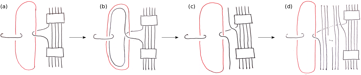
Figure 1. $-1$ and $-t$ twists on a fixed string which links one other string.

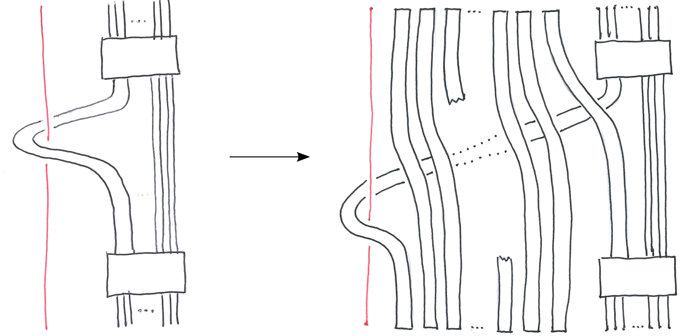
Figure 2. A $-t$ twist on a fixed string which links a ribbon of parallel strings.

We will use the following simplified version of Thurston’s Hyperbolic Dehn Surgery Theorem, which follows from Chapters 4 and 5 of [28], see also [2, 21].

Theorem 1.

Let $L=L_{1}\cup\dots\cup L_{n}$ be a link in $S^{3}$ such that $M:=S^{3}\setminus L$ is a complete hyperbolic 3-manifold of finite volume, $r_{i}=b_{i}/a_{i}$ be a sequence of rationals with $a_{i}^{2}+b_{i}^{2}\to\infty$, and $M_{i}$ be the sequence of 3-manifolds obtained by Dehn filling $L_{1}$ with surgery coefficients $r_{i}$. Then $M_{i}$ converges geometrically to $M$, and the convergence is non-trivial in the sense that $M_{i}$ and $M$ are distinct for all $i$, so that there are infinitely many distinct 3-manifolds $M_{i}$.

2. The braids $\beta_{q}$

Recall that the positive permutation braid $\beta\in B_{n}$ defined by a permutation $\pi\in S_{n}$ is the unique $n$-braid which induces the permutation $\pi$ on its strings, and which has the properties that every pair of strings crosses at most once, and that every crossing is in the positive sense (we adopt the convention, following Birman [4], that a braid crossing is positive if the left string crosses over the right one). Thus a diagram of $\beta$ can be constructed by drawing the $1^{\text{st}}$ to the $n^{\text{th}}$ strings in order, with the $i^{\text{th}}$ string going from position $i$ to position $\pi(i)$ and passing underneath any intervening strings which have already been drawn.

The following definition is from theorem 2.1 of [17], and the fact that the braids defined are of pseudo-Anosov type is contained in the proof of theorem 2.3 of the same paper. (There the braids $\beta^{\prime}_{q}$ are also defined for $q\in(1/3,1/2)$, but this is done in a different way and, since we are only interested in limits as $q\to 0$, is not relevant here.) Here and throughout the paper, when we write a positive rational number as $m/n$, we will always assume that $m$ and $n$ are coprime and positive.

Definition 2 (The braids $\beta^{\prime}_{q}$).

Let $q=m/n\in{{\mathbb{Q}}}\cap(0,1/3]$. The braid $\beta^{\prime}_{q}\in B_{n+2}$ is the positive permutation braid (see Figure 3) defined by the cyclic permutation

(2) $$\pi_{q}(r)=\begin{cases}r+m&\text{ if }1\leq r\leq n-3m+1,\\ r+m+1&\text{ if }n-3m+2\leq r\leq n-2m+1,\\ 2n-2m+4-r&\text{ if }n-2m+2\leq r\leq n-m+1,\\ n-2m+2&\text{ if }r=n-m+2,\\ n+3-r&\text{ if }n-m+3\leq r\leq n+2.\end{cases}$$

It is helpful to organize the strings of $\beta^{\prime}_{q}$ in ribbons of parallel strings: the 5 cases of (2) yield, in order:

• A ribbon of width $n-3m+1$ which moves $m$ places to the right.

• A ribbon of width $m$ which moves $m+1$ places to the right, thus leaving the target in position $n-2m+2$ unassigned.

• A ribbon of width $m$ which is sent to the final $m$ target positions with a half twist.

• A ‘rogue’ string, which ends at the unassigned target in position $n-2m+2$.

• A ribbon of width $m$, which is sent to the first $m$ target positions with a half twist.

Figure 3. The braid $\beta^{\prime}_{m/n}\in B_{n+2}$.

Definition 3 (The braids $\beta_{q}$).

It will be convenient for us to conjugate the braids $\beta^{\prime}_{q}$ by a half twist of the final $m$ strings, thereby turning the half twist on the final ribbon into a full twist, and removing the half twist on the penultimate ribbon: these conjugated braids will be denoted $\beta_{q}$ (Figure 4). (The braids $\beta_{q}$ can be seen as circular braids, as shown on the right of the figure, with each string other than the rogue one rotating around the circle by either $m$ or $m+1$ positions. This point of view motivates constructions later in the paper — see Definitions 6 and 10.)

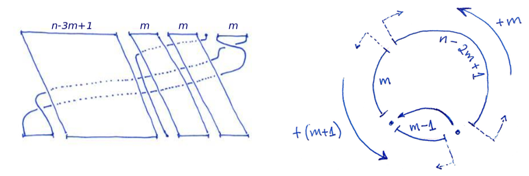
Figure 4. The braid $\beta_{m/n}\in B_{n+2}$, and as a circular braid.

3. Pseudo-Anosov convergence to the tight horseshoe

The tight horseshoe map [9] $\varphi_{0}\colon S\to S$ is a 2-sphere homeomorphism which can be obtained by collapsing the horizontal and vertical gaps in the invariant Cantor set of Smale’s horseshoe map [25]. In order to define it directly, we start with its sphere $S$ of definition, which is obtained by making identifications along the sides of a unit square $\Sigma$ as depicted in Figure 5. Infinitely many segments along the boundary of $\Sigma$, two of length $1/2^{i}$ for each $i\geq 0$, are folded in half (so that the points of each segment, other than the center point, are identified in pairs). The top and right edges of $\Sigma$ are each a single folded segment, and the other segments are arranged on the left and bottom sides in decreasing order of length from the top left and bottom right vertices respectively. The fold segment endpoints, together with the bottom left corner, are identified to a single point $\infty$. It can be shown (see for example [11]) that the space $S$ so obtained is a topological sphere (and, in fact, that the Euclidean structure on $\Sigma$ induces a well defined conformal structure on $S$).

Figure 5. The sphere $S$ of definition of the tight horseshoe map.

To define the tight horseshoe map, let $F\colon\Sigma\to\Sigma$ be the (discontinuous and non-injective) map defined by

$$F(x,y)=\begin{cases}(2x,\,y/2)&\text{ if }x\leq 1/2,\\ (2-2x,\,1-y/2)&\text{ if }x>1/2.\end{cases}$$

That is, $F$ stretches $\Sigma$ by a factor 2 horizontally, contracts it by a factor $1/2$ vertically, and maps its left half to its bottom half, and its right half, with a flip, to its top half. The identifications on $\Sigma$ are precisely those needed to make $F$ continuous and injective, so that it defines a homeomorphism $\varphi_{0}\colon S\to S$, the tight horseshoe map. (It is an example of a generalized pseudo-Anosov map [10]: it has (horizontal and vertical) unstable and stable invariant foliations, but these foliations have infinitely many $1$-pronged singularities — at the centers of the fold segments — accumulating on an ‘$\infty$-pronged singularity’ corresponding to the fold segment endpoints and the bottom left vertex.)

For each $q=m/n\in(0,1/3]\cap{{\mathbb{Q}}}$, let $\varphi_{q}\colon S^{2}\to S^{2}$ be a pseudo-Anosov homeomorphism in the mapping class of the $(n+3)$-marked sphere defined by $\beta_{q}$. The convergence of $\varphi_{q}$ to $\varphi_{0}$ as $q\to 0$ is an immediate consequence of results from [6]. The following statement is a summary of the relevant parts of theorems 5.19 and 5.31 of that paper.

Theorem 4.

There is a continuously varying family $\{\chi_{t}\colon S^{2}\to S^{2}\}_{t\in(\sqrt{2},2]}$ of homeomorphisms of the standard 2-sphere, with the properties that:

1. $\chi_{2}$ is topologically conjugate to $\varphi_{0}$; and

2. there is a decreasing function $t\colon(0,1/3]\cap{{\mathbb{Q}}}\to(\sqrt{2},2)$, satisfying $t(q)\to 2$ as $q\to 0$, such that $\chi_{t(q)}$ is topologically conjugate to $\varphi_{q}$ for each $q$.

Remark 5.

A brief discussion of the ideas surrounding Theorem 4 may be helpful to the reader. Boyland [5] defined the braid type of a period $n$ orbit $P$ of an orientation-preserving disk homeomorphism $f\colon D^{2}\to D^{2}$ to be the isotopy class of $f\colon D^{2}\setminus P\to D^{2}\setminus P$, up to conjugacy in the mapping class group of the $n$-punctured disk: the braid type can therefore be described — although not uniquely — by a braid $\beta_{P}\in B_{n}$. He further defined the forcing relation, a partial order on the set of braid types: one braid type forces another if every homeomorphism which has a periodic orbit of the former braid type also has one of the latter. The forcing relation therefore describes constraints on the order in which periodic orbits can appear in parameterized families of homeomorphisms.

If $f$ is Smale’s horseshoe map, then standard symbolic techniques associate a code $c_{P}\in\{0,1\}^{n}$ to a period $n$ orbit $P$. This coding establishes a correspondence between the non-trivial periodic orbits of $f$ and those of the affine unimodal tent maps $T_{t}\colon[0,1]\to[0,1]$ defined for $t\in(1,2]$ by

$$T_{t}(x)=\min(2+t(x-1),t(1-x)),$$

whose periodic orbits are likewise coded in a standard way. The braids $\beta^{\prime}_{q}$ of Definition 2 — or, more accurately, the braids $\beta^{\prime}_{q}$ for $q\in(0,1/2)\cap\mathbb{Q}$ alluded to before the definition — are precisely the pseudo-Anosov braids describing braid types of horseshoe periodic orbits $P_{q}$ which are quasi-one-dimensional, in the sense that the braid types that they force are exactly those corresponding to the periodic orbits of the tent map $T_{t(q)}$ which has kneading sequence $c_{P_{q}}^{\infty}$ [17].

Another way to view the braids $\beta_{q}^{\prime}$ is as the braids of horseshoe periodic orbits $P_{q}$ whose mapping class is pseudo-Anosov and whose associated train tracks are the simplest possible: if the $1$-gons about the orbit points are ignored, then the union of the remaining edges is an arc. This means that the only singularities of the invariant foliations of $\varphi_{q}$ are 1-prongs at points of the orbit and an $n$-prong at $\infty$, where $q=m/n$. This is what makes the orbits $P_{q}$ quasi-one-dimensional: the induced map on the reduced train track (which is an interval) is a unimodal interval map.

One way to construct the pseudo-Anosov map in a mapping class is as a factor of the natural extension of a corresponding train track map. In [6], a similar method is used to construct a measurable pseudo-Anosov homeomorphism from the natural extension of each tent map $T_{t}$ with $t>\sqrt{2}$: these form the continuously varying family $\chi_{t}$ of Theorem 4. They are pseudo-Anosov maps if and only if the kneading sequence of the tent map is periodic and is the horseshoe code of one of the braids $\beta_{q}^{\prime}$, i.e., if and only if $t=t(q)$ for some $q\in(0,1/2)\cap\mathbb{Q}$, and in this case $\chi_{t(q)}$ is topologically conjugate to $\varphi_{q}$.

Theorem 4 also provides limits of the pseudo-Anosov homeomorphisms $\varphi_{q}$ as $q$ tends to an irrational $\xi$, or to a rational $r$ either from above or from below (the image of $t$ is discrete). All such limits are generalized pseudo-Anosov homeomorphisms.

4. Convergence of mapping tori

Let $\nu=\ell/m\in[0,1)\cap{{\mathbb{Q}}}$, and consider the corresponding sequence $(q^{(\nu)}_{k})_{k\geq 3}$ of rationals defined by $q^{(\nu)}_{k}=\frac{m}{km+\ell}$. By the description of the ribbon structure of the braids $\beta_{q}$ in Section 2, the braid $\beta_{q^{(\nu)}_{k}}$ is as depicted in Figure 4, with the first ribbon having width $(k-3)m+\ell+1$ and the others having width $m$.

In this section we will show that, for each $\nu$, the mapping tori $M_{q^{(\nu)}_{k}}$ converge geometrically as $k\to\infty$ to a hyperbolic manifold ${\widehat{M}}_{\nu}$ of finite volume. In the following section, we will prove that the set $\{{\widehat{M}}_{\nu}\colon\nu\in[0,1)\cap{{\mathbb{Q}}}\}$ is infinite.

The crucial observation is that the sequence of mapping tori $M_{q^{(\nu)}_{k}}$ can be obtained from a single finite-volume hyperbolic 3-manifold ${\widehat{M}}_{\nu}$ by Dehn filling one of its cusps with a sequence of distinct surgery coefficients $r_{k}$: it therefore follows from Theorem 1 that the sequence of mapping tori converges geometrically to ${\widehat{M}}_{\nu}$.

The manifolds ${\widehat{M}}_{\nu}$ are themselves mapping tori, corresponding to braids $\gamma_{\nu}$ which are obtained from $\beta_{q^{(\nu)}_{3}}=\beta_{m/(3m+\ell)}$ by adding one additional string on the left. This additional string is chosen precisely in order that ${\widehat{M}}_{\nu}$ is the geometric limit of the sequence $M_{q^{(\nu)}_{k}}$ (see the proof of Theorem 7).

Definition 6 (The braids $\gamma_{\nu}$).

Let $\nu=\ell/m\in[0,1)\cap{{\mathbb{Q}}}$. The braid $\gamma_{\nu}\in B_{3m+\ell+3}$ is obtained from $\beta_{m/(3m+\ell)}$ by adding a fixed string on the left, which links with the final width $m$ ribbon of $\beta_{m/(3m+\ell)}$ but not with the other strings, as depicted in Figure 6. (In the circular representation of Figure 4, this corresponds to adding a fixed string, not linking the rogue string, through the center of the circle.)

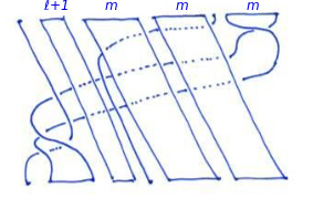
Figure 6. The braid $\gamma_{\ell/m}$.

That $\gamma_{\nu}$ is a pseudo-Anosov braid follows from the fact that $\beta_{m/(3m+\ell)}$ is. (Any reducing curve $C$ would bound a disk $D$ containing at least two but not all of the punctures associated with the strings of $\gamma_{\nu}$. $D$ cannot contain the puncture associated to the fixed string, since then its image would also contain that puncture but a different set of the other punctures; it cannot contain a proper subset of the other punctures, since then $\beta_{m/(3m+\ell)}$ would be reducible; and it cannot contain all of the other punctures since the associated strings link with the fixed string.) Therefore ${\widehat{M}}_{\nu}:=S^{3}\setminus({\overline{\gamma}}_{\nu}\cup A)$ (where $A$ is the braid axis) is a finite volume hyperbolic $3$-manifold with $3$ cusps.

Theorem 7.

Let $\nu\in[0,1)\cap{{\mathbb{Q}}}$ and $k\geq 1$. Dehn filling the cusp of ${\widehat{M}}_{\nu}$ corresponding to the fixed string of $\gamma_{\nu}$ with surgery coefficient $1/k$ yields $M_{q^{(\nu)}_{k+3}}$.

Proof.

It is immediate from Figure 2 that performing a $-k$ twist on the component $R$ of ${\overline{\gamma}}_{\nu}\cup A$ corresponding to the fixed string increases the width of the first ribbon of $\gamma_{\nu}$ from $\ell+1$ to $km+\ell+1$. By (1), this changes the surgery coefficient on $R$ to $r_{1}(R)=1/(-k+1/(1/k))=\infty$, so that it can be erased, yielding the closure of the braid $\beta_{m/((k+3)m+\ell)}=\beta_{q_{k+3}^{(\nu)}}$ (see Figure 4). That is, Dehn filling $R$ with surgery coefficient $1/k$ yields $M_{q_{k+3}^{(\nu)}}$ as required. ∎

The following corollary is now immediate from Theorem 1.

Corollary 8.

For each $\nu\in[0,1)\cap{{\mathbb{Q}}}$ the sequence $M_{q^{(\nu)}_{k}}$ converges geometrically to ${\widehat{M}}_{\nu}$.

5. Infinitely many limit manifolds

Figure 7 is a plot of the volumes of the limit manifolds ${\widehat{M}}_{\nu}$ against $\nu$, generated by SnapPy [8]. The points in red are those for which $\nu$ is of the form $i/(i+1)$. In this section we show how all of the corresponding manifolds ${\widehat{M}}_{i/(i+1)}$ can be obtained by Dehn filling a cusp of another hyperbolic $3$-manifold $M$ with a sequence of distinct surgery coefficients, so that, again by Theorem 1, there are infinitely many distinct limit manifolds ${\widehat{M}}_{i/(i+1)}$ (which converge geometrically to $M$ as $i\to\infty$).

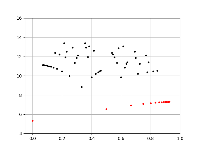
Figure 7. Volumes of the limit manifolds ${\widehat{M}}_{\nu}$ (for $\nu$ with denominator $\leq 14$).

Remarks 9.

1. Other apparently convergent sequences in Figure 7 correspond to similar sequences $\nu_{i}$, such as $\nu_{i}=1/i$ and $\nu_{i}=i/(2i+1)$.

2. The volume $5.333489\ldots$ of ${\widehat{M}}_{0}$ suggests that it may be the magic manifold. To see that this is indeed the case, consider the braids depicted in Figure 8, each representing the 3-manifold obtained by removing the braid closure together with its axis from $S^{3}$. The braid on the left is $\gamma_{0/1}$, representing ${\widehat{M}}_{0}$, while the one on the right represents the magic manifold (see for example Figure 3 of [19]). The operations converting each braid to the next are either twists on components of the associated links or braid conjugacies, and therefore leave the 3-manifolds unchanged. Specifically, these operations are, in order: conjugacy by $\sigma_{4}^{-1}$; a $+3$ twist on the red component (see Figure 1 (d) and (a)); conjugacy by $\sigma_{2}$; a $+1$ twist on the braid axis; and conjugacy by $\sigma_{1}\sigma_{2}$.

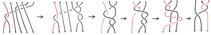
Figure 8. ${\widehat{M}}_{0}$ is the magic manifold.

The manifold $M$ is obtained from the $10$-braid $\delta$ of the following definition (see Figure 9), whose closure ${\overline{\delta}}$ is a three-component link. Note that the blue and green strings in the figure form a braid conjugate to $\gamma_{0/1}$ (the conjugacy $\sigma_{1}^{-1}\sigma_{2}^{-1}\sigma_{3}^{-1}\sigma_{4}^{-1}\sigma_{5}^{-1}$ moves the fixed string from the left to the right of the braid diagram), and to this braid has been added a $4$-string braid which ‘shadows’ the blue strings. It is not obvious a priori — at least, not to the authors — that Dehn filling the ‘black’ cusp of the resulting hyperbolic $3$-manifold should yield the manifolds ${\widehat{M}}_{i/(i+1)}$: rather, the braid $\delta$ was found experimentally using SnapPy [8].

Definition 10.

Let $\delta=\sigma_{6}\sigma_{5}\sigma_{4}\sigma_{3}\sigma_{9}\sigma_{8}\sigma_{8}\sigma_{9}\sigma_{7}\sigma_{6}\sigma_{5}\sigma_{4}\sigma_{3}\sigma_{2}\sigma_{1}\sigma_{8}\sigma_{7}\sigma_{6}\sigma_{5}\sigma_{4}\sigma_{3}\sigma_{2}\sigma_{1}\sigma_{8}\sigma_{6}\in B_{10}$.

It can be checked, using the implementation [18] of the Bestvina-Handel algorithm for train tracks of surface homeomorphisms [3] that $\delta$ is pseudo-Anosov, with its train track and image train track as shown in Figure 10. The corresponding relative pseudo-Anosov homeomorphism therefore has 1-pronged singularities at the marked points corresponding to the blue and green strings of Figure 9, a $4$-pronged singularity at $\infty$, and regular points at the black marked points. Therefore $M:=S^{3}\setminus({\overline{\delta}}\cup A)$ (where $A$ is the braid axis) is a finite volume hyperbolic 3-manifold with 4 cusps.

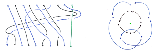
Figure 9. The braid $\delta\in B_{10}$.

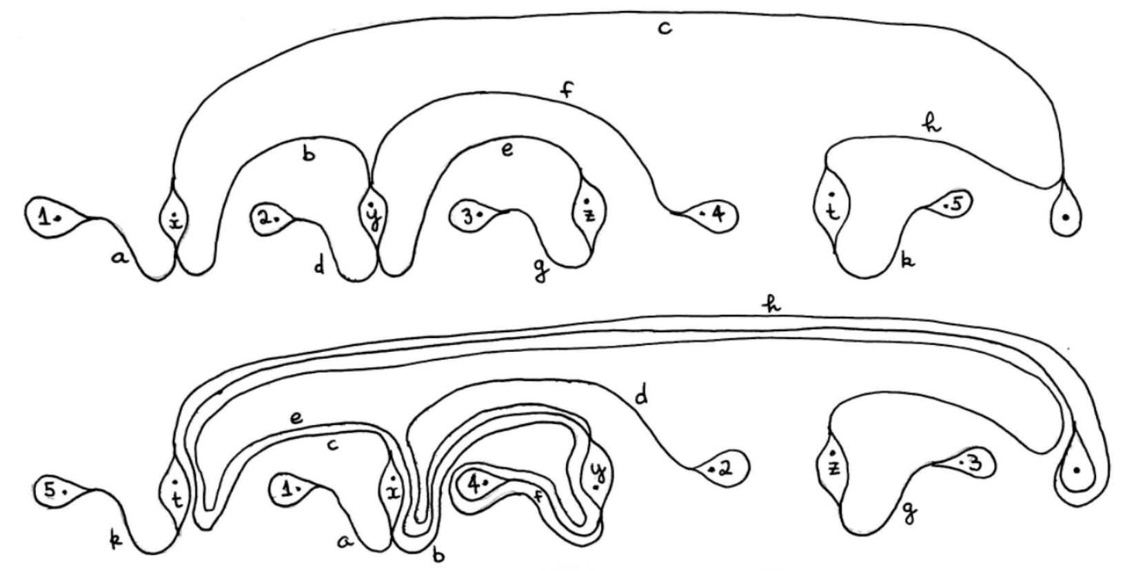
Figure 10. An invariant train track for $\delta$, and its image.

Theorem 11.

Let $i\geq 1$. Dehn filling the cusp of $M$ corresponding to the black strings of Figure 9 with surgery coefficient $-4+1/i$ yields ${\widehat{M}}_{i/(i+1)}$.

Proof.

The left hand side of Figure 11 depicts a braid $\zeta$, which is $\delta$ together with an extra fixed string shown in red. We write $B$ and $R$ for the black and red components of ${\overline{\zeta}}$, which are unknotted. We need to show that filling $B$ with coefficient $r_{0}(B)=-4+1/i$ and $R$ with coefficient $r_{0}(R)=\infty$ (i.e. erasing $R$ from the link ${\overline{\zeta}}\cup A$) yields the $3$-manifold ${\widehat{M}}_{i/(i+1)}$.

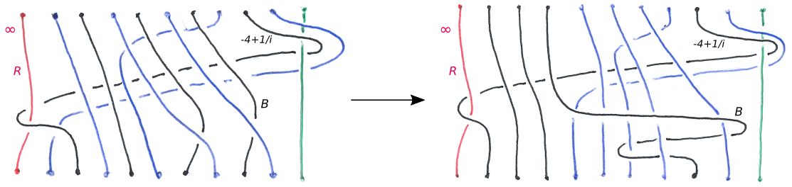
Figure 11. Conjugating $\zeta$ to prepare it for a $+3$ twist on $R$.

The braid on the right hand side of the figure is obtained by conjugating by $\sigma_{7}^{-2}\sigma_{2}^{-1}\sigma_{4}^{-1}\sigma_{3}^{-1}\sigma_{6}^{-1}\sigma_{5}^{-1}\sigma_{4}^{-1}$. Referring to Figure 1, performing a $+3$ twist on $R$ yields the braid on the left of Figure 12, and a conjugacy by $\sigma_{6}^{-1}\sigma_{7}$ gives the braid on the right hand side of the figure. By (1), the updated surgery coefficients are:

$$r_{1}(R) = 1/(3+1/r_{0}(R))=1/3,\text{ and}$$

$$r_{1}(B) = r_{0}(B)+3=-1+1/i,$$

since $\operatorname{lk}(B,R)=1$.

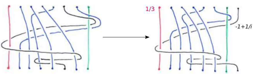
Figure 12. A $+3$ twist on $R$, followed by a conjugacy.

Performing a $+1$ twist on the braid axis $A$ yields the braid on the left hand side of Figure 13, which a further conjugacy by $\sigma_{7}\sigma_{6}\sigma_{5}\sigma_{4}\sigma_{3}\sigma_{2}\sigma_{1}\sigma_{1}\sigma_{2}\sigma_{3}\sigma_{4}\sigma_{5}\sigma_{6}\sigma_{7}$ — to pull the black string around — reduces to the right hand side of the figure. (Here and in Figure 14, the parts of the blue strings which participate in the full twist have not been drawn, to clarify the diagrams.) The red component $R$ and the black component $B$ are now unlinked. The revised surgery coefficients are

$$r_{2}(R) = 1/3+1=4/3,\text{ and}$$

$$r_{2}(B) = -1+1/i+1=1/i,$$

since $\operatorname{lk}(A,R)=\operatorname{lk}(A,B)=1$.

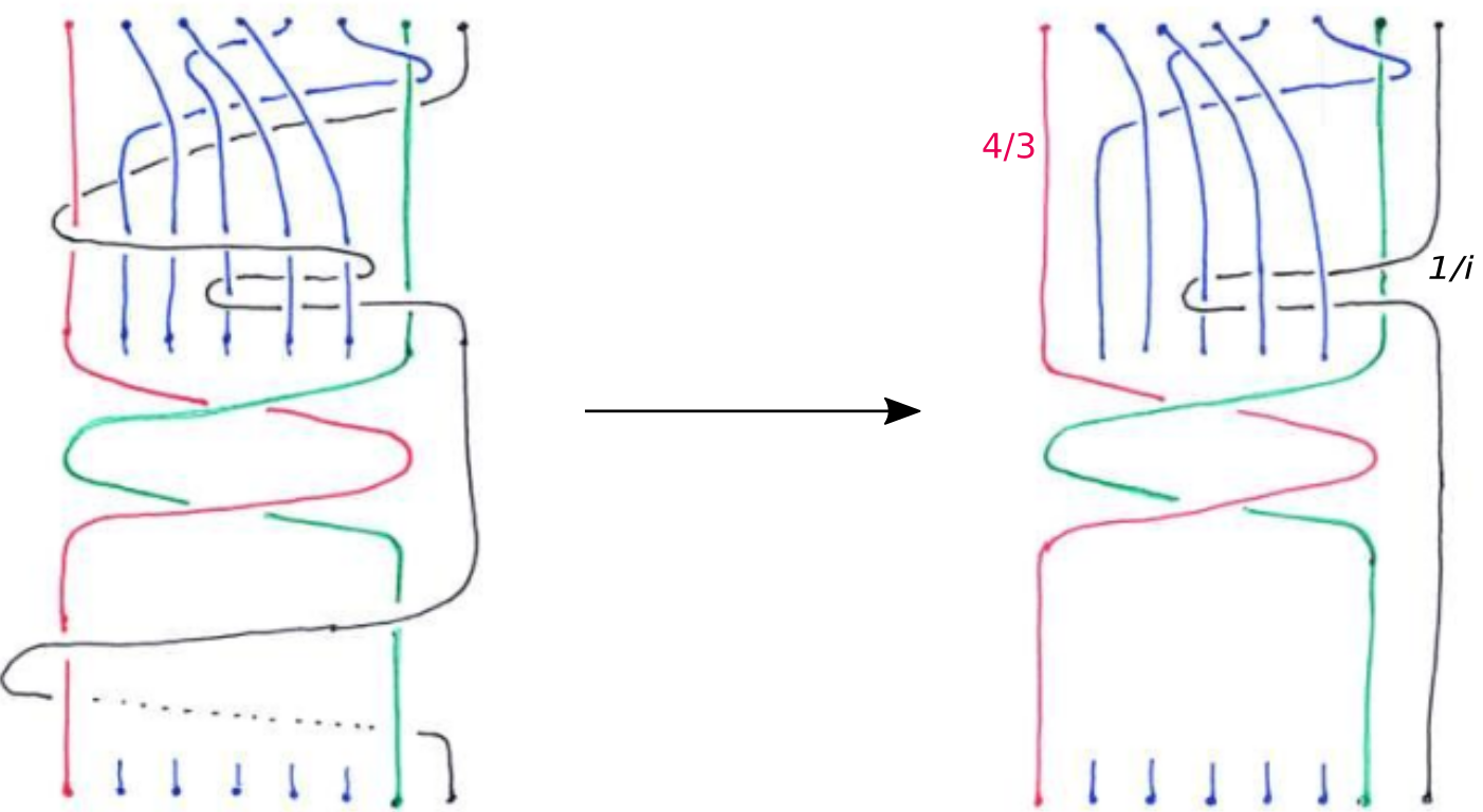
Figure 13. A $+1$ twist on the braid axis $A$, followed by a conjugacy.

We can now carry out the surgery on $B$. Performing a $-i$ twist on $B$ yields the braid of Figure 14 (in which the ribbon contains $i-1$ parallel strings). The surgery coefficient of $B$ is

$$r_{3}(B)=\frac{1}{-i+1/(1/i)}=\infty,$$

so that it can be removed (and is not shown in Figure 14). Because $R$ and $B$ are unlinked, the surgery coefficient of $R$ is unchanged: $r_{3}(R)=r_{2}(R)=4/3$.

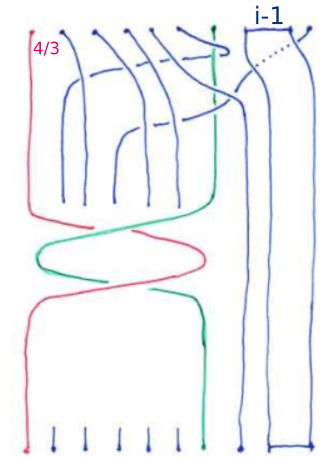
Figure 14. A $-i$ twist on $B$ changes its surgery coefficient to $\infty$.

We next perform a $-1$ twist on $A$, which produces the braid on the left hand side of Figure 15, and changes the surgery coefficient of $R$ to $r_{4}(R)=1/3$. A $-3$ twist on $R$ therefore changes its coefficient to $\infty$, so that it can be erased: this results in the braid on the right hand side of Figure 15, in which each of the four ribbons contains $i-1$ parallel strings.

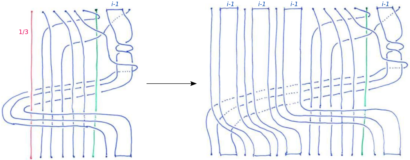
Figure 15. A $-1$ twist on $A$ followed by a $-3$ twist on $R$.

To complete the proof, we exhibit a braid conjugacy between the braid on the right hand side of Figure 15 and the braid $\gamma_{i/(i+1)}$ — that is, the braid of Figure 6 with all four ribbons containing $i+1$ parallel strings. (This conjugacy was discovered computationally, using sliding circuit set methods [15, 16] for small values of $i$ and extrapolating: the braids $\gamma_{i/(i+1)}$ have small sliding circuit sets but large ultra summit sets [14].) Two successive conjugacies are shown in Figure 16. Here the first, second, and fourth ribbons have been enlarged by incorporating an additional parallel string, so that they each contain $i$ parallel strings.

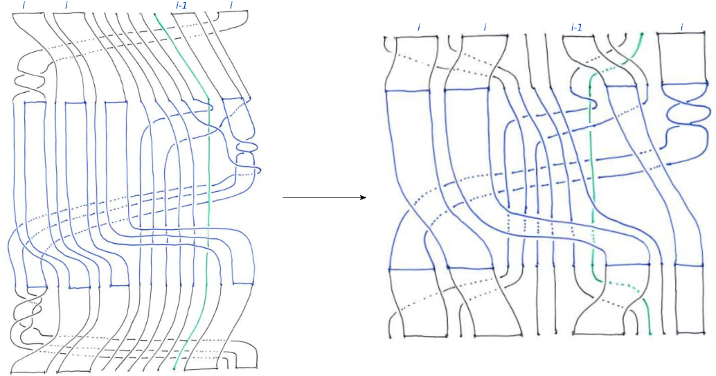
Figure 16. Successive conjugacies on the right hand side of Figure 15.

Simplifying the braid on the right hand side of Figure 16 by isotopy of the strings yields the braid on the left hand side of Figure 17. Again, we have incorporated additional parallel strings into ribbons, so that the first two ribbons contain $i+1$ parallel strings, and the other two contain $i$ parallel strings. A final conjugacy which moves the green string to the left, underneath all of the other strings, gives the braid on the right hand side of the figure, and incorporating additional parallel strings into the rightmost two ribbons yields $\gamma_{i/(i+1)}$ as required.

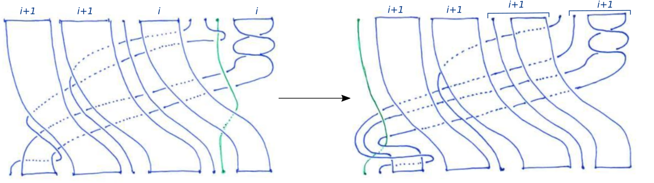
Figure 17. A simplified diagram of the right hand side of Figure 16, followed by a conjugacy.

∎

Corollary 12.

The sequence ${\widehat{M}}_{i/(i+1)}$ converges geometrically to $M$ as $i\to\infty$, and there are infinitely many distinct hyperbolic 3-manifolds ${\widehat{M}}_{i/(i+1)}$.

6. Acknowledgements

The authors are grateful for the support of FAPESP grant 2016/25053-8 and CAPES grant 88881.119100/2016-01. AdC is partially supported by CNPq grant PQ 302392/2016-5. JGM is partially supported by Spanish Project MTM2016-76453-C2-1-P and FEDER.

The authors appreciate the very helpful comments of an anonymous referee.

References

- [1] I. Agol, Ideal triangulations of pseudo-Anosov mapping tori, Topology and geometry in dimension three, Contemp. Math., vol. 560, Amer. Math. Soc., Providence, RI, 2011, pp. 1–17. MR 2866919
- [2] R. Benedetti and C. Petronio, Lectures on hyperbolic geometry, Universitext, Springer-Verlag, Berlin, 1992. MR 1219310
- [3] M. Bestvina and M. Handel, Train-tracks for surface homeomorphisms, Topology 34 (1995), no. 1, 109–140. MR 1308491
- [4] J. Birman, Braids, links, and mapping class groups, Princeton University Press, Princeton, N.J., 1974, Annals of Mathematics Studies, No. 82. MR 0375281
- [5] P. Boyland, Topological methods in surface dynamics, Topology Appl. 58 (1994), no. 3, 223–298. MR 1288300
- [6] P. Boyland, A. de Carvalho, and T. Hall, Natural extensions of unimodal maps: virtual sphere homeomorphisms and prime ends of basin boundaries, Geom. Topol. (in press).
- [7] A. Casson and S. Bleiler, Automorphisms of surfaces after Nielsen and Thurston, London Mathematical Society Student Texts, vol. 9, Cambridge University Press, Cambridge, 1988. MR 964685
- [8] M. Culler, N. Dunfield, M. Goerner, and J. Weeks, SnapPy, a computer program for studying the geometry and topology of -manifolds, Available at http://snappy.computop.org [downloaded: 20/12/18], 2018.
- [9] A. de Carvalho, Extensions, quotients and generalized pseudo-Anosov maps, Graphs and patterns in mathematics and theoretical physics, Proc. Sympos. Pure Math., vol. 73, Amer. Math. Soc., Providence, RI, 2005, pp. 315–338. MR 2131019
- [10] A. de Carvalho and T. Hall, Unimodal generalized pseudo-Anosov maps, Geom. Topol. 8 (2004), 1127–1188. MR 2087080
- [11] by same author, Paper folding, Riemann surfaces and convergence of pseudo-Anosov sequences, Geom. Topol. 16 (2012), no. 4, 1881–1966. MR 2975296
- [12] B. Farb, C. Leininger, and D. Margalit, Small dilatation pseudo-Anosov homeomorphisms and 3-manifolds, Adv. Math. 228 (2011), no. 3, 1466–1502. MR 2824561
- [13] A. Fathi, F. Laudenbach, and V. Poénaru, Travaux de Thurston sur les surfaces, Astérisque, vol. 66, Société Mathématique de France, Paris, 1979, Séminaire Orsay, With an English summary. MR 568308
- [14] V. Gebhardt, A new approach to the conjugacy problem in Garside groups, J. Algebra 292 (2005), no. 1, 282–302. MR 2166805
- [15] V. Gebhardt and J. González-Meneses, The cyclic sliding operation in Garside groups, Math. Z. 265 (2010), no. 1, 85–114. MR 2606950
- [16] by same author, Solving the conjugacy problem in Garside groups by cyclic sliding, J. Symbolic Comput. 45 (2010), no. 6, 629–656. MR 2639308
- [17] T. Hall, The creation of horseshoes, Nonlinearity 7 (1994), no. 3, 861–924.
- [18] by same author, Trains, an implementation of the Bestvina-Handel algorithm, Available at http://pcwww.liv.ac.uk/maths/tobyhall/software/, 2009.
- [19] E. Kin and M. Takasawa, Pseudo-Anosovs on closed surfaces having small entropy and the Whitehead sister link exterior, J. Math. Soc. Japan 65 (2013), no. 2, 411–446. MR 3055592
- [20] C. McMullen, Renormalization and 3-manifolds which fiber over the circle, Annals of Mathematics Studies, vol. 142, Princeton University Press, Princeton, NJ, 1996. MR 1401347
- [21] W. Neumann and D. Zagier, Volumes of hyperbolic three-manifolds, Topology 24 (1985), no. 3, 307–332. MR 815482
- [22] J-P. Otal, The hyperbolization theorem for fibered 3-manifolds, SMF/AMS Texts and Monographs, vol. 7, American Mathematical Society Providence RI; Société Mathématique de France Paris, 2001, Translated from the 1996 French original by Leslie D. Kay. MR 1855976
- [23] R. Penner, Bounds on least dilatations, Proc. Amer. Math. Soc. 113 (1991), no. 2, 443–450. MR 1068128
- [24] D. Rolfsen, Knots and links, Mathematics Lecture Series, vol. 7, Publish or Perish Inc., Houston TX, 1990, Corrected reprint of the 1976 original. MR 1277811
- [25] S. Smale, Differentiable dynamical systems, Bull. Amer. Math. Soc. 73 (1967), 747–817. MR 0228014
- [26] W. Thurston, On the geometry and dynamics of diffeomorphisms of surfaces, Bull. Amer. Math. Soc. (N.S.) 19 (1988), no. 2, 417–431. MR 956596
- [27] by same author, Hyperbolic structures on 3-manifolds, II: surface groups and 3-manifolds which fiber over the circle, arXiv:9801045v1 [math.GT] (1998).
- [28] by same author, The geometry and topology of three-manifolds, Available at http://library.msri.org/books/gt3m/ [downloaded: 20/12/18], 2002.