Phase-amplitude formalism for ultra-narrow shape resonances

Abstract

We apply Milne’s phase-amplitude representation [W. E. Milne, Phys. Rev. 35, 863 (1930)] to a scattering problem involving disjoint classically allowed regions separated by a barrier. Specifically, we develop a formalism employing different sets of amplitude and phase functions — each set of solutions optimized for a separate region — and we use these locally adapted solutions to obtain the true value of the scattering phase shift and accurate tunneling rates for ultra-narrow shape resonances. We show results for an illustrative example of an attractive potential with a large centrifugal barrier.

I Introduction

An integral representation for scattering phase shifts based on the phase-amplitude formalism was recently derived by the present authors Shu et al. (2018). Although the main result of Ref. Shu et al. (2018) is fully general, the computational approach was restricted to a single (infinite) classically allowed region; thus, in the presence of a barrier, our previous method can only be employed for energies above the barrier. We now extend the phase-amplitude formalism Milne (1930) to scattering energies below the top of the barrier, and we provide a method for characterizing shape resonances. We pay special attention to the case of a large barrier delimiting a deep inner well capable of holding long-lived resonances. A variety of methods Hazi and Taylor (1970); Mandelshtam et al. (1993); Babb and Du (1990); Sidky and Ben-Itzhak (1999); Gibson et al. (1998); Mrugała (2008) have been developed for tunneling resonances; however, the regime of ultra-narrow resonances ($\Gamma\lll E_{\text{res}}$) still presents computational difficulties Sidky and Ben-Itzhak (1999); Gibson et al. (1998); Mrugała (2008). The phase-amplitude approach presented in this work overcomes this obstacle, as it yields the scattering phase shift expressed in terms of quantities obeying a simple energy dependence and allows the extraction of highly accurate resonance widths.

Milne’s phase-amplitude method Milne (1930) has a long history and has been used extensively in atomic physics Greene et al. (1982); Yoo and Greene (1986); Robicheaux et al. (1987); Raoult and Balint-Kurti (1988); Fourré and Raoult (1994); Bohn (1994); Burke et al. (1998); Bohn and Julienne (1999); Ch. Jungen and Texier (2000); Bar-Shalom et al. (2001); Crubellier and Luc-Koenig (2006); Lecomte and Raoult (2007); Zhao et al. (2012); Hall et al. (2013); Price and Greene (2018). However, its wealth of advantages is still being explored Kiyokawa (2015); Shu et al. (2018); Cariglia et al. (2018); Lidsey . In this study we exploit the relationship between the solutions of the radial Schrödinger equation and those of the envelope equation (which is equivalent with Milne’s amplitude equation). In particular, we develop an approach for extending the phase function outside its domain of smoothness, which makes it possible to combine solutions that are locally adapted in each classically allowed region and thus bridge them across the barrier. Making use of our new results, we can now extend the applicability of the integral representation in Ref. Shu et al. (2018) to scattering energies below the top of the barrier, which allows us to analyze ultra-narrow shape resonances.

This article is organized as follows. Section II gives the theoretical description of our phase-amplitude approach, which makes it possible to separate the background and resonant contributions to the scattering phase shift; see Sec. III.2. The resonance widths are obtained in Sec. III.3, and results for an illustrative example are presented in Sec. IV. Concluding remarks are given in Sec. V.

II Theory: envelope equation approach

We consider the scattering of two structureless, spinless particles with a spherically symmetric potential $V(R)$. The radial Schrödinger equation reads

$$\Psi^{\prime\prime}=U\Psi,\qquad U=2\mu\big{(}V_{\rm eff}-E\big{)},$$ (1)

where $V_{\rm eff}(R)=V(R)+\frac{\ell(\ell+1)}{2\mu R^{2}}$ is the effective potential, $\mu$ is the reduced mass of the two particles undergoing scattering, and $E=\frac{k^{2}}{2\mu}>0$ is the energy in the center-of-mass frame. Atomic units are used throughout.

II.1 The envelope equation

As in our previous work Shu et al. (2018) (see also Ref. Schief (1997); Moyo and Leach (2000); Kiyokawa (2015)), the Schrödinger equation is replaced by the envelope equation,

$$\rho^{\prime\prime\prime}=4U\!\rho^{\prime}+2U^{\prime}\!\rho.$$ (2)

A particular solution $\rho(R)$ and its corresponding phase $\theta(R)$ can be used to parametrize the physical wave function,

$$\psi(R)=\sqrt{\rho(R)}\sin[\theta(R)-\theta(0)],$$ (3)

and to obtain the scattering phase shift,

$$\delta_{\ell}=\ell\textstyle\frac{\pi}{2}-\theta(0).$$ (4)

This result relies on the smoothness of $\rho(R)$ and $\theta(R)$ in the asymptotic region, which is ensured using the computational approach of Ref. Shu et al. (2018). Namely, $\rho(R)$ is initialized at $R=\infty$ according to the asymptotic boundary condition

$$\rho(R)\xrightarrow{R\to\infty}1,$$

and is propagated inward. The envelope function $\rho(R)$ is then used to obtain $\theta(R)$ by integrating

$$\theta^{\prime}=\frac{k}{\rho}.$$ (5)

The phase function will thus obey the asymptotic behavior

$$\theta(R)\xrightarrow{R\to\infty}kR.$$

Our main goal is computing the phase $\theta(R)$ at $R=0$, which yields the phase shift $\delta_{\ell}$ in Eq. (4). In our previous work Shu et al. (2018) we presented a method suitable for the case of a single classically allowed region extending to infinity. However, if the effective potential $V_{\text{eff}}(R)$ has a barrier, and if the scattering energy is below the top of the barrier, the direct propagation (numerical integration) of the outer phase $\theta$ into the inner potential well is no longer feasible, as we explain below.

An example of a potential with a large barrier is depicted in Fig. 1. For energies $0<E<E_{\text{top}}$, where $E_{\text{top}}$ is the height of the barrier, two classically allowed regions exist, which are separated by the barrier. We thus divide the radial domain in two regions, as shown in Fig. 1. The turning point on the inner side of the barrier, $R_{\rm in}(E)$, is the boundary between the inner and the outer regions. The latter includes the classically forbidden region under the barrier and the entire asymptotic domain.

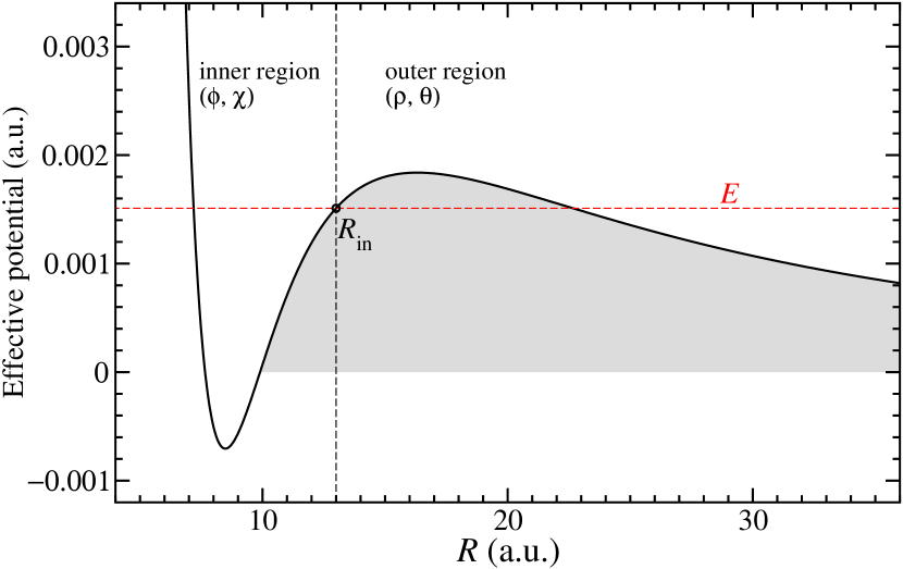
Figure 1: A representative effective potential which has a sufficiently deep well at short range, delimited by a large barrier (indicated by the shaded area). The dashed vertical line at the turning point $R_{\text{in}}$ separates the inner and outer regions.

The outer envelope and phase, $\rho$ and $\theta$, are propagated inward through the asymptotic region and through the barrier, using the method we presented in Ref. Shu et al. (2018). We remark that the classically forbidden region under the barrier does not pose any difficulties. However, the envelope $\rho(R)$ increases quasi-exponentially, as $R$ decreases through the barrier region; thus, $\rho(R_{\text{in}})$ will be very large. This can be easily understood if we write $\rho=f^{2}+g^{2}$, where $f$ and $g$ are solutions of the radial equation which obey the asymptotic behavior $f(R)\sim\sin(kR)$ and $g(R)\sim\cos(kR)$. According to their definition, $f$ and $g$ are linearly independent; hence, one solution (say, $g$), or both of them, must increase through the barrier, as $R$ decreases towards $R_{\text{in}}$. Thus, the dominant solution ($g$) will dictate the behavior of the envelope inside the inner well, where we have $\rho(R)=g^{2}(R)$ to a very good approximation; consequently, for $R<R_{\text{in}}$, the envelope has an oscillatory behavior with (nearly) vanishing minima at the nodes of $g$, and exceedingly large values at the anti-nodes. This would cause severe difficulties if $\theta(R)$ were propagated inside the inner well ($R<R_{\text{in}}$). Indeed, when integrating Eq. (5), the minima of $\rho$ yield a series of sharp spikes for the integrand $\frac{k}{\rho(R)}$, which cannot be handled numerically. Therefore, the inner region has to be tackled separately (independently of the outer region), and the two regions need to be bridged together, in order to obtain $\theta(0)$.

II.2 Linear decomposition of envelope solutions

As is well known, the general solution of Milne’s amplitude equation can be expressed Pinney (1950); Eliezer and Gray (1976); Reid and Ray (1980); Korsch and Laurent (1981); Yoo and Greene (1986) in terms of solutions of the radial equation (1). Equivalently, the general solution of the envelope equation (2) can be written as

$$\rho=a\phi^{2}+b\chi^{2}+2c\phi\chi,$$ (6)

where $\phi$ and $\chi$ are linearly independent solutions of Eq. (1). The coefficients $a$, $b$ and $c$ are free in general, but they can be chosen to obey the constraint

$$\left(ab-c^{2}\right)W^{2}=k^{2},$$ (7)

with $W$ the Wronskian of $\phi$ and $\chi$. The constraint above is directly related to an invariant of the envelope equation, as explained in Appendix A. We emphasize that $\phi^{2}$, $\chi^{2}$ and $\phi\chi$ are particular solutions of the envelope equation ; see Ref. Shu et al. (2018). Moreover, $W\neq 0$ ensures that they do indeed form a fundamental set of solutions of the envelope equation; a rigorous proof is given in Appendix A, thereby justifying that Eq. (6) represents the general solution of Eq. (2). The linear decomposition (6) together with the constraint (7) play a pivotal role in our work, as we show next.

II.3 Matching equations

Inside the inner region ($0<R<R_{\rm in}$) we employ two linear independent solutions ($\phi,\ \chi$) of the radial equation (1), and we ensure $\phi(R)\to 0$ when $R\to 0$, such that $\phi$ is the regular solution. We now use Eq. (6) to express the outer envelope $\rho$ in terms of $\phi$ and $\chi$. We emphasize that the numerical methods employed for $\phi$, $\chi$ and $\rho$ must ensure their well defined energy dependence; this will be inherited by the coefficients $a(E)$, $b(E)$ and $c(E)$, which are obtained from the matching conditions

$$a\phi^{2}+b\chi^{2}+2c\phi\chi = \rho$$

$$a\phi\phi^{\prime}+b\chi\chi^{\prime}+c\big{(}\phi\chi\big{)}^{\prime} = \textstyle\frac{1}{2}\rho^{\prime}$$ (8)

$$a\Big{(}\phi^{\prime}\Big{)}^{2}+b\Big{(}\chi^{\prime}\Big{)}^{2}+2c\phi^{\prime}\chi^{\prime} = \textstyle\frac{1}{2}\rho^{\prime\prime}-U\!\rho.$$

The coefficients $a$, $b$ and $c$ are independent of the matching point; thus, in principle, the matching conditions could be imposed anywhere; however, in practice, the matching point should be located near $R_{\text{in}}$. Indeed, the outer phase $\theta$ cannot be propagated inside the inner well, as explained in Sec. II.1. Conversely, if $\phi$ and $\chi$ were propagated outside the inner well, they would increase through the barrier and become linearly dependent. Hence, as depicted in Fig. 1, the most convenient choice for the matching point is the inner turning point $R_{\text{in}}$.

The $3\times 3$ linear system of equations (8) is solved in an elementary way; first, we find that the determinant $\Delta$ is given by a simple expression, $\Delta=W^{3}\neq 0$, with $W$ the (nonvanishing) Wronskian of $\phi$ and $\chi$; then, the coefficients $a$, $b$ and $c$ are obtained as the unique solution,

$$W^{2}a = \rho\left(\chi^{\prime}-\frac{\chi\rho^{\prime}}{2\rho}\right)^{2}+\frac{k^{2}\chi^{2}}{\rho}$$

$$W^{2}b = \rho\left(\phi^{\prime}-\frac{\phi\rho^{\prime}}{2\rho}\right)^{2}+\frac{k^{2}\phi^{2}}{\rho}$$ (9)

$$W^{2}c = -\rho\left(\phi^{\prime}-\frac{\phi\rho^{\prime}}{2\rho}\right)\left(\chi^{\prime}-\frac{\chi\rho^{\prime}}{2\rho}\right)-\frac{k^{2}\phi\chi}{\rho},$$

with $\phi$, $\chi$ and $\rho$ evaluated at the matching point. The coefficients $a$, $b$ and $c$ can now be used to obtain the phase shift.

II.4 Extracting the scattering phase shift

According to Eq. (4), in order to find the phase shift, we need to extend the outer phase into the inner region; this can be accomplished using Eqs. (5)–(7), as shown in Appendix B. The key result is Eq. (B), which yields the outer phase at $R=0$. For the sake of clarity, we set $W=k$ in Eq. (B) to simplify the expression of the outer phase,

$$\theta(0)=\theta_{*}-\pi N_{*}-\alpha_{*}+\arctan(c),$$

where $\theta_{*}\equiv\theta(R_{\text{in}})$ stems from the outer-region propagation, $N_{*}$ is the number of nodes of $\chi$ in the inner region, and

$$\alpha_{*}=\arctan(c+az_{*}),$$ (10)

with $z_{*}=\frac{\phi(R_{\text{in}})}{\chi(R_{\text{in}})}$. Finally, we substitute $\theta(0)$ in Eq. (4) to find

$$\delta_{\ell}=\ell\frac{\pi}{2}-\theta_{*}+\pi N_{*}+\alpha_{*}+\arctan(-c).$$ (11)

The phase shift is thus expressed in terms of the coefficients $a$ and $c$ that we obtained in the previous section. The last term in the equation above, namely $\arctan[-c(E)]$, yields the width $\Gamma$ for ultra-narrow resonances, as we shall see in Sec. III.3. However, in preparation for extracting $\Gamma$, we first employ a phase-amplitude parametrization for the inner solutions $\phi$ and $\chi$ in the next section, which yields simpler expressions for the coefficients $a$, $b$ and $c$.

II.5 Locally adapted solutions in the inner region

Although $\phi$ and $\chi$ can be obtained as numerical solutions of the radial equation, we prefer instead to employ the phase-amplitude method in the inner region (similar to the outer region). This will make it possible to express the coefficients $a,\ b$ and $c$ in terms of an inner-region phase which has a smooth energy dependence.

Let $\varrho$ denote the envelope inside the inner region, and $\beta$ the corresponding phase function,

$$\beta(R)\equiv\!\int_{0}^{R}\!\!\frac{q}{\varrho(r)}dr,$$ (12)

where the parameter $q>0$ can be chosen conveniently. We emphasize that the inner and outer envelope functions ($\varrho$ and $\rho$, respectively) are different solutions on the envelope equation; consequently, the phase functions $\beta$ and $\theta$ differ nontrivially. A simple optimization procedure Shu et al. is employed in the inner region to ensure the smoothness of $\varrho$ and $\beta$, which we now use to construct $\phi$ and $\chi$,

$$\phi=\sqrt{\varrho}\sin\beta,\qquad\chi=\sqrt{\varrho}\cos\beta.$$ (13)

We remark that Eq. (12) ensures $\beta=0$ at $R=0$. Thus, $\phi$ is the regular solution, as desired; moreover, Eqs. (12) and (13) yield the Wronskian $W=\phi^{\prime}\chi-\phi\chi^{\prime}=q$. We now substitute Eqs. (12) and (13) in Eq. (9) to rewrite the coefficients $a,\ b$ and $c$ in terms of the inner phase $\beta$,

$$a \;=\; u\,\cos^{2}(\beta+\eta)+\varepsilon\cos^{2}\beta$$

$$b \;=\; u\,\sin^{2}(\beta+\eta)+\varepsilon\sin^{2}\beta$$ (14)

$$c \;=\; -u\,\sin(\beta+\eta)\cos(\beta+\eta)-\varepsilon\sin\beta\cos\beta.$$

In the equations above and hereafter, $\beta=\beta(R_{\text{in}})$. The inner and outer envelopes (and their derivatives) at the matching point also appear in Eq. (14) via the quantities $\eta$, $u$ and $\varepsilon$,

$$\cot\eta=\frac{\varrho}{2q}\left(\frac{\varrho^{\prime}}{\varrho}-\frac{\rho^{\prime}}{\rho}\right),$$ (15)

$$u=\frac{\rho}{\varrho}\csc^{2}\eta,\qquad\varepsilon=\frac{\varrho}{\rho}\left(\frac{k}{q}\right)^{2}.$$ (16)

The three parameters above are interrelated, as they obey the relationship $u\varepsilon=\Big{(}\frac{k}{q}\csc\eta\Big{)}^{2}$.

The equations above render the phase shift $\delta_{\ell}$ in Eq. (11) expressed exclusively in terms of quantities obtained from the phase-amplitude formalism; indeed, $N_{*}=\operatorname{nint}[\beta(R_{\text{in}})/\pi]$, where $\operatorname{nint}[\cdots]$ stands for nearest integer, while making use of $z_{*}=\frac{\phi(R_{\text{in}})}{\chi(R_{\text{in}})}=\tan\beta(R_{\text{in}})$, $\alpha_{*}$ in Eq. (10) reads

$$\alpha_{*} = \arctan(c+a\tan\beta)$$

$$= \arctan\left[-u\sin(\eta)\cos(\beta+\eta)\sec(\beta)\right]$$

$$= -\arctan\left(\frac{\rho\cos(\beta+\eta)}{\varrho\sin\eta\cos\beta}\right).$$

Finally, we remark that the equations in this section remain valid if the inner envelope $\varrho$ has residual oscillations; thus, strictly speaking, the inner envelope $\varrho$ need not be smooth. However, the optimization method Shu et al. that we devised for honing in on the smooth envelope is advantageous in practice, provided that a well defined $E$-dependence for $\varrho$ is ensured; indeed, attention must be paid when employing optimization, as the inner envelope will be initialized with values which are numerical functions of energy.

III theory: envelope rescaling and resonance widths

III.1 Envelope rescaling

As explained in Sec. II.1, the outer envelope follows a quasi-exponential behavior under the barrier when $E<E_{\text{top}}$, which yields $\rho(R_{\text{in}})\ggg 1$. Hence, the coefficients $a$, $b$ and $c$ can reach exceedingly large values and have to be rescaled; indeed, $\rho(R)$ is rescaled during its propagation through the barrier, in order to avoid numerical overflow. Therefore, at the end of the propagation, the value of $\rho(R_{\text{in}})$, and thus $u$ and $\varepsilon$, will be represented logarithmically.

We remark that, although $a$, $b$ and $c$ are independent of the matching point, the parameters $\eta$, $u$ and $\varepsilon$ do depend on its location. Hence, if $u$ (or $\rho$ itself) were used as scaling factor, the rescaled coefficients would depend on the matching point. Although this would not entail any difficulty, it is possible to rescale the coefficients such that they do remain formally independent of the matching point. Namely, we choose the quantity $\upsilon\equiv u+\varepsilon$ as the scaling factor; from Eq. (14) we find

$$\upsilon=u+\varepsilon=a+b,$$ (18)

which is independent of the matching point, and we define the scaled coefficients according to

$$\tilde{a}\equiv\frac{a}{\upsilon},\qquad\tilde{b}\equiv\frac{b}{\upsilon},\qquad\tilde{c}\equiv\frac{c}{\upsilon}.$$ (19)

Equation (14) can now be recast as

$$\tilde{a} \;=\; \tilde{u}\cos^{2}(\beta+\eta)+\tilde{\varepsilon}\cos^{2}\beta$$

$$\tilde{b} \;=\; \tilde{u}\sin^{2}(\beta+\eta)+\tilde{\varepsilon}\sin^{2}\beta$$ (20)

$$\tilde{c} \;=\; -\tilde{u}\sin(\beta+\eta)\cos(\beta+\eta)-\tilde{\varepsilon}\sin\beta\cos\beta,$$

where the scaled parameters

$$\tilde{u}\equiv\frac{u}{\upsilon},\qquad\tilde{\varepsilon}\equiv\frac{\varepsilon}{\upsilon}$$

obey the simple relationship

$$\tilde{u}+\tilde{\varepsilon}=1,$$

which render the scaled coefficients of the order of unity.

III.2 Ultra-narrow resonances

For scattering energies $E$ sufficiently lower than $E_{\text{top}}$, we enter the regime of ultra-narrow resonances, characterized by $\tilde{\varepsilon}\sim\rho^{-2}(R_{\text{in}})\lll\tilde{u}\approx 1$. This simplifies greatly the expressions of the scaled coefficients; indeed, Eq. (20) becomes

$$\tilde{a}(E) \;\approx\; \cos^{2}\beta_{\text{full}}(E)$$

$$\tilde{b}(E) \;\approx\; \sin^{2}\beta_{\text{full}}(E)$$ (21)

$$\tilde{c}(E) \;\approx\; -\sin\beta_{\text{full}}(E)\cos\beta_{\text{full}}(E),$$

where the phase

$$\beta_{\text{full}}\equiv\beta+\eta$$ (22)

represents the full contribution from the inner region and the barrier; see Appendix C.

Ultra-narrow resonances correspond to metastable (quasibound) states, and their positions ($E_{\text{res}}$) can be obtained as the roots of $\beta_{\text{full}}(E)=N\pi$ with $N$ a positive integer. Hence, the resonance positions are the minima of $\tilde{b}(E)$, i.e., the roots of $\sin\beta_{\text{full}}=0$. Note that we also have $\tilde{c}(E)=0$ at $E=E_{\text{res}}$. We remark that methods which are suitable for bound states can be used to find the positions $E_{\text{res}}$ of quasi-bound states. On the other hand, the vanishingly small widths ($\Gamma$) of such resonances are difficult to obtain.

In preparation for the next section, where the resonance width $\Gamma$ will be extracted, we first rewrite $\delta_{\ell}$ in Eq. (11) as a sum of background and resonant contributions, and we analyze the resonant phase shift in detail. For scattering energies sufficiently lower than $E_{\text{top}}$, the large barrier plays the role of a repulsive wall. Therefore, the inner region is inaccessible (unless $E\approx E_{\text{res}}$) and we identify the background term,

$$\delta_{\ell}^{\rm bg}(E)\equiv\ell\frac{\pi}{2}-\theta_{*}(E),$$ (23)

which is given by the outer phase $\theta_{*}(E)=\theta(E;R_{\text{in}})$, with $R_{\text{in}}$ playing the same role as $R=0$ in Eq. (4). The remaining terms in Eq. (11) give the contribution of the inner region, which we interpret as the resonant part of the phase shift,

$$\delta_{\ell}^{\rm res}(E)\equiv\pi N_{*}(E)+\alpha_{*}(E)\arctan[-c(E)].$$ (24)

To simplify our notation, we shall omit the subscript $\ell$ for the remainder of this article, and we rewrite Eq. (11) as

$$\delta(E)=\delta^{\rm bg}(E)+\delta^{\rm res}(E).$$

As we explain next, the resonant phase shift is very nearly constant between resonances, $\delta^{\text{res}}(E)\approx N\pi$. Thus, we have

$$\delta(E)\stackrel{{\scriptstyle{\scriptscriptstyle\text{mod}\,\pi}}}{{=}}\delta^{\text{bg}}(E),\qquad E\neq E_{\text{res}},$$ (25)

which confirms the interpretation of $\delta^{\text{bg}}$ in Eq. (23) as the background phase shift.

In order to understand the energy dependence of $\delta^{\rm res}(E)$, we first recall that $N_{*}(E)$ is an integer-valued step function; secondly, in the regime of ultra-narrow resonances we have $\alpha_{*}(E)\approx\arctan(\pm\infty)=\pm\frac{\pi}{2}$, due to $u\sim\rho\to\infty$ in Eq. (II.5). Similarly, $\arctan[c(E)]\approx\arctan(\pm\infty)=\pm\frac{\pi}{2}$, and thus the last two terms in Eq. (24) yield $\alpha_{*}-\arctan(c)\approx\pm\pi$ or zero. Consequently, $\delta^{\rm res}(E)$ is to an excellent approximation a piecewise constant function, whose values are integer multiples of $\pi$. More precisely, $\delta^{\rm res}(E)$ follows a stepwise behavior, increasing sharply by $\pi$ at each resonance, as we explain next.

The behavior of $\delta^{\rm res}(E)$ can be fully elucidated by a more detailed analysis of the terms in Eq. (24). First, the discontinuous steps of $N_{*}(E)=\operatorname{nint}[\beta/\pi]$ when $\beta\stackrel{{\scriptstyle{\scriptscriptstyle\text{mod}\,\pi}}}{{=}}\frac{\pi}{2}$ are irrelevant, as each step ($+\pi$) due to $\pi N_{*}(E)$ is canceled by an opposite ($-\pi$) step given by $\alpha_{*}(E)=\arctan(c+a\tan\beta)$, due to $\tan\beta$ jumping from $+\infty$ to $-\infty$. Second, we observe that both $\tilde{a}(E)$ and $\tilde{c}(E)$ will vanish when $\cos\beta_{\text{full}}=0$; see Eq. (21). The roots of $\cos\beta_{\text{full}}=0$ are interspersed between the roots of $\sin\beta_{\text{full}}=0$, i.e, the zeros of $b(E)$. The latter give the resonance positions $E_{\text{res}}$, while the common zeros of $a(E)$ and $c(E)$ are completely unremarkable despite the fact that both $\alpha_{*}(E)$ and $\arctan[c(E)]$ in Eq. (24) vary rapidly in their vicinity; indeed, using the definition (10) of $\alpha_{*}$ and the constraint $1+c^{2}=ab$ (see Eq. (7) with $W=k$), we find that the last two terms in Eq. (24) cancel nearly perfectly,

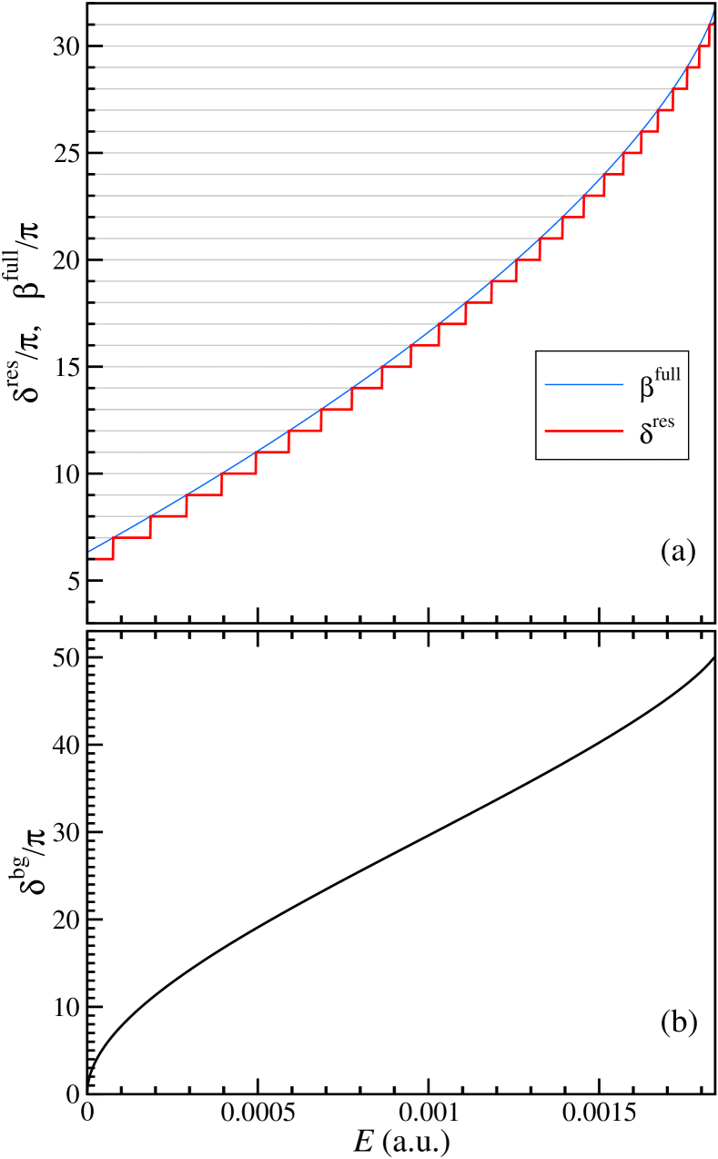
Figure 2: Energy dependence of the resonance phase shift $\delta^{\text{res}}$ (thick red line) and $\beta_{\text{full}}=\beta+\eta$ (thin blue line) in the top panel (a), and background phase shift $\delta^{\text{bg}}$ in the bottom panel (b). The full phase shift $\delta=\delta^{\text{bg}}+\delta^{\text{res}}$ is shown in Fig. 3(c), where the resonance positions are indicated. The results were obtained using the potential energy (32).

$$\alpha_{*} - \arctan(c)=\arctan(c+az_{*})-\arctan(c)$$

$$= \arctan\left(\frac{az_{*}}{1+c^{2}+acz_{*}}\right)=\arctan\left(\frac{z_{*}}{b+cz_{*}}\right)\approx 0.$$

This expression vanishes because $b\approx\infty$ when $\sin\beta_{\text{full}}\not\approx 0$. Finally, one is left with the only possible explanation for the stepwise behavior of $\delta^{\rm res}(E)$. Namely, it stems solely from the last term in Eq. (24),

$$\arctan[-c(E)]=-\arctan\big{[}\upsilon(E)\tilde{c}(E)\big{]}.$$

Indeed, at $E_{\text{res}}$ we have $c=0$ (and $b\approx 0$) due to $\sin\beta_{\text{full}}=0$. Moreover, the derivative $\dot{c}\equiv\frac{dc}{dE}$ is very large at $E=E_{\text{res}}$,

$$\dot{c}(E_{\text{res}})=\upsilon(E_{\text{res}})\dot{\tilde{c}}(E_{\text{res}})=-\upsilon(E_{\text{res}})\dot{\beta}_{\text{full}}(E_{\text{res}}).$$ (26)

Hence, as $E$ increases within a narrow window around $E_{\text{res}}$, $c(E)$ decreases rapidly (practically from $+\infty$ to $-\infty$), which yields a rapid increase of $\arctan[-c(E)]$ from $-\frac{\pi}{2}$ to $+\frac{\pi}{2}$. This is in agreement with the well known signature of scattering resonances; namely, the increase by $\pi$ of the phase shift at each resonance, as depicted in Fig. 2(a).

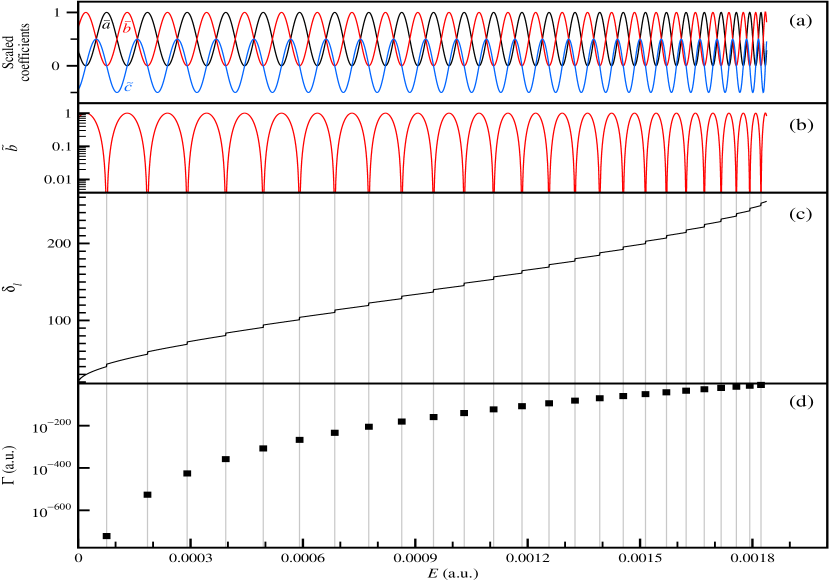
Figure 3: Energy dependence of the scaled coefficients (a), semilog plot of $\tilde{b}$ (b), phase shift $\delta_{\ell}$ (c), and resonance widths (d). The vertical lines mark the positions of the resonances.

III.3 Resonance widths

We now extract the widths of ultra-narrow resonances, while the case of broad resonances (e.g., above-barrier resonances) will be discussed in Sec. IV.1. As is well known, the scattering phase shift $\delta(E)$ increases rapidly when $E\approx E_{\text{res}}$, and its derivative $\dot{\delta}(E)\equiv\frac{d\delta}{dE}$ has a sharp maximum at $E_{\rm res}$. We thus analyze $\dot{\delta}$ to extract the resonance width $\Gamma$. For ultra-narrow resonances, the phase shift can be easily separated into background and resonant contributions, as shown in the previous section. Moreover, in the immediate vicinity of a narrow resonance, the background term is nearly constant and we neglect it. Therefore, we need only consider the resonant phase shift in Eq. (24). Specifically, its derivative reads

$$\dot{\delta}^{\text{res}}\equiv\frac{d\delta^{\text{res}}}{dE}\approx\frac{d}{dE}\big{[}\!-\!\arctan c(E)\big{]}=-\frac{\dot{c}(E)}{1+c^{2}(E)},$$ (27)

where we used $\dot{N}_{*}=0$ and $\dot{\alpha}_{*}\approx 0$. In order to extract the resonance width $\Gamma$, we employ the linear approximation

$$c(E)\approx\dot{c}_{\rm res}(E-E_{\rm res}),$$ (28)

with $\dot{c}_{\text{res}}\equiv\dot{c}(E_{\text{res}})$. The linearization (28) is essentially exact within a sufficiently narrow window $\Delta E$; at the same time, the strong inequality $\Delta E\ggg\Gamma$ also holds. Thus, the line shapes of ultra-narrow resonances are accurately given by

$$\dot{\delta}^{\text{res}}(E)\approx-\frac{\dot{c}_{\text{res}}}{1+\big{(}\dot{c}_{\text{res}}\big{)}^{2}\big{(}E-E_{\text{res}}\big{)}^{2}}.$$ (29)

Comparing this result to the familiar Breit–Wigner expression,

$$\dot{\delta}_{\text{BW}}(E)=\frac{\frac{\Gamma}{2}}{\big{(}E-E_{\text{res}}\big{)}^{2}+\left(\frac{\Gamma}{2}\right)^{2}},$$ (30)

we identify the resonance width,

$$\frac{2}{\Gamma}=-\dot{c}_{\text{res}}.$$ (31)

Making use of Eq. (26), we can express the resonance width in terms of the scaled coefficients,

$$\frac{2}{\Gamma}=-\upsilon_{\text{res}}\dot{\tilde{c}}_{\text{res}}=\upsilon_{\text{res}}\dot{\beta}^{\text{full}}_{\text{res}},$$

with $\dot{\tilde{c}}_{\text{res}}\equiv\dot{\tilde{c}}(E_{\text{res}})$ and $\upsilon_{\text{res}}\equiv\upsilon(E_{\text{res}})$. We emphasize that the vanishingly small value of $\Gamma$ for ultra-narrow resonances stems from the huge value of the scaling factor $\upsilon\approx u$, which in turn is due to the exponential increase of the envelope through the barrier. Finally, we remark that the linearization (28) was used only within a very narrow window $\Delta E$ around $E_{\text{res}}$ to facilitate the formal comparison of the Breit–Wigner formula (30) with Eq. (29). However, we evaluate the energy derivative $\dot{\tilde{c}}(E_{\text{res}})$ using a high order method for numerical differentiation based on Chebyshev polynomials covering a wide energy interval. Thus, in order to attain high accuracy, we account fully for the nonlinear behavior of $\tilde{c}(E)$ and $\beta^{\text{full}}(E)$.

IV Results and discussion

As an illustrative example, we consider the potential energy employed in our previous work Shu et al. (2018),

$$V(R)=C_{\rm wall}\,e^{-\frac{R}{R_{\text{wall}}}}\;-\;\frac{C_{3}}{R^{3}+R_{\rm core}^{3}},$$ (32)

with $C_{\rm wall}=10$, $R_{\rm wall}=1$, $R_{\rm core}=5$ and $C_{3}=18$ (all in atomic units), and the reduced mass $\mu=\frac{m}{2}$, where $m$ is the mass of ⁸⁸Sr. Although $V(R)$ is barrierless, the effective potential, $V_{\text{eff}}=V+\frac{\ell(\ell+1)}{2\mu R^{2}}$, will have a centrifugal barrier for $0<\ell\lessapprox 557$. We are interested in the case of a large barrier, and thus a sufficiently high value for $\ell$ will be used; namely, $\ell=500$. As depicted in Fig. 1, the effective potential has a large centrifugal barrier and a sufficiently deep well at short range holding a large number of shape resonances. Hence, our example is a suitable representative for potentials which posses ultra-narrow shape resonances.

Figure 2 shows the energy dependence of $\delta^{\rm bg}(E)$ and $\delta^{\rm res}(E)$, as well as $\beta_{\text{full}}(E)$. It is readily apparent in Fig. 2(a) that the resonant phase shift is constant between resonances, $\delta^{\text{res}}(E)\approx N\pi$, with the integer $N$ increasing by unity for each resonance, as we discussed in Sec. III.2.

The phase $\beta_{\text{full}}(E)$ has a smooth energy dependence, as shown in Figure 2(a), which explains the simple oscillatory behavior of the scaled coefficients in Fig. 3(a). The unscaled coefficients follow the same oscillatory behavior, albeit modulated by the strongly varying amplitude $\upsilon(E)\approx u(E)$, which is dominated by the quasi-exponential behavior of the outer envelope $\rho(E;R_{\text{in}})$. However, the scaling (19) was not introduced to merely simplify the plot in Fig. 3(a). Indeed, the scaling factor $\upsilon(E)$ and the scaled coefficient $\tilde{c}(E)$ proved instrumental in extracting the resonance width $\Gamma$, as discussed in Sec. III.3.

A semilog plot of $\tilde{b}(E)$ is shown in Fig. 3(b), while the phase shift is depicted in Fig. 3(c). As discussed in Sec. III.2, the nearly vanishing minima of $\tilde{b}(E)$ and hence of $b(E)$ signify resonances, whose positions are marked by the vertical lines; the widths $\Gamma$ are plotted in the bottom panel (d).

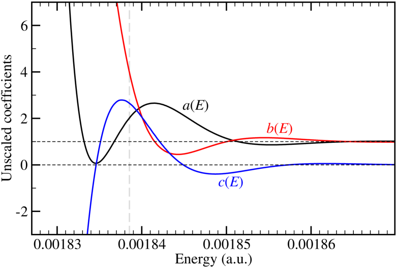
Figure 4: Energy dependence of the coefficients $a(E)$, $b(E)$ and $c(E)$ in the vicinity of $E_{\text{top}}$, which is marked by the vertical dashed line. As the energy $E$ increase above the barrier, the coefficients $a(E)$ and $b(E)$ converge to unity, while $c(E)$ converges to zero; these limits are marked by horizontal dashed lines.

IV.1 Above-barrier resonances

For scattering energies just above the barrier, the situation is similar to the case $E<E_{\text{top}}$; namely, a globally smooth envelope does not exist ($\varrho\neq\rho$). Hence, it is again advantageous to combine locally adapted solutions for the inner and outer regions. However, global smoothness will be recovered very quickly when the energy increases above the barrier; this is apparent in Fig. 4, which shows the behavior of the unscaled coefficients ($a$, $b$, $c$) for energies below and above $E_{\text{top}}$. The limits $a(E)\approx b(E)\to 1$ and $c(E)\to 0$, which correspond to the globally smooth envelope $\varrho=\rho$, are eventually attained at high energies. We remark that the nonexistence of a globally smooth envelope ($\varrho\neq\rho$) for energies just above the barrier is closely related to quantum reflection Maitra and Heller (1996); Côté et al. (1997); Segev et al. (1997); Côté et al. (1998), which only vanishes at energies sufficiently high above the barrier (when a globally smooth envelope does exist).

As is well known, shape resonances may occur for energies just above the barrier. Such resonances are rather broad, and are in stark contrast with the ultra-narrow resonances described in the previous section. We now discuss briefly an example of a broad above-barrier resonance, which will shed more light on ultra-narrow resonances.

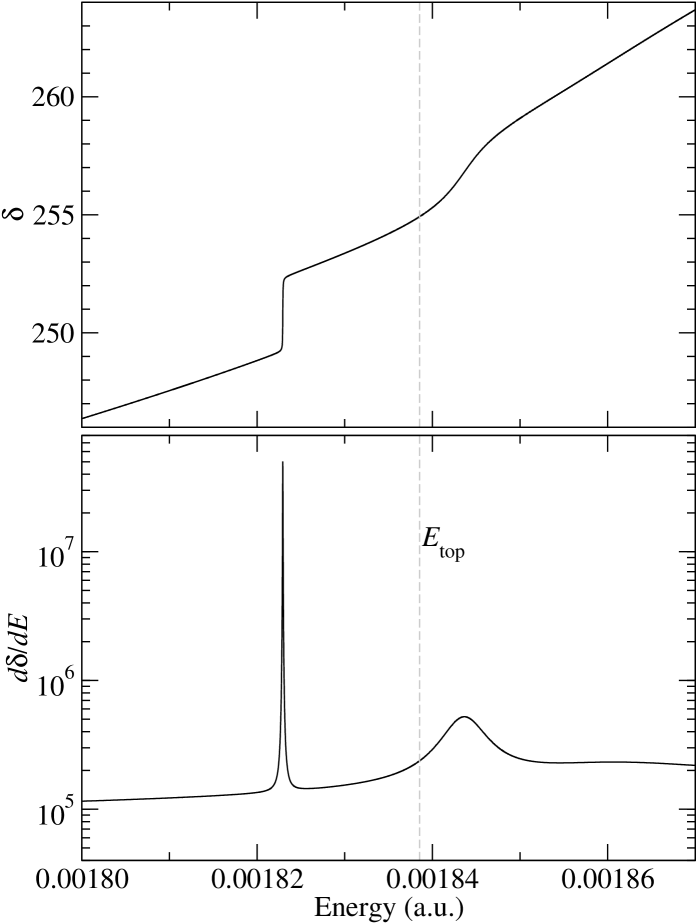
Figure 5: Energy dependence of the phase shift $\delta$ and its derivative $\dot{\delta}$ for scattering energies near the top of the barrier $E_{\text{top}}$ (marked by a vertical dashed line). The sharp feature is the first resonance below the top of the barrier. The broad resonance above the barrier is also visible (especially in the lower panel).

For $E>E_{\text{top}}$, a convenient choice for the matching point is $R_{\text{top}}$ (the location of the barrier top). However, as the energy increases above the barrier, the boundary between the inner and outer regions becomes arbitrary; hence, the interpretation of the outer-region contribution (23) as the background phase shift loses its meaning. Thus, although our method is still useful for computing the phase shift, the extraction of the resonance width (and position) must be performed by fitting the resonance line-shape using the Breit–Wigner formula. The fitting procedure must also include an energy dependent background, as it cannot be neglected in this case; indeed, for broad resonances, $\delta^{\text{bg}}(E)$ may vary significantly within $\Delta E\sim\Gamma$.

Figure 5 shows the behavior of the phase shift $\delta(E)$ and its derivative $\dot{\delta}(E)$ for energies $E$ near the top of the barrier. Two resonances are readily apparent; namely, the first resonance under the barrier, which is sufficiently narrow to be analyzed as explained in Sec. III.3, and a broad resonance above the barrier. The latter is resolved by fitting its lineshape, as mentioned above. Specifically, we employ

$$\dot{\delta}_{\text{fit}}(E)=\dot{\delta}_{\text{BW}}(E)+\dot{\delta}^{\text{bg}}_{\text{fit}}(E),$$

with $\dot{\delta}_{\text{BW}}(E)$ given in Eq. (30) and a low degree polynomial for the background term $\dot{\delta}^{\text{bg}}_{\text{fit}}(E)$ to extract the resonance position $E_{\rm res}=1.84362\times 10^{-3}\text{ a.u.}$ and width $\Gamma=5.628\times 10^{-6}\text{ a.u.}$

We emphasize that the fitting procedure can only be used when resonances are sufficiently broad for their lineshapes to be resolved via a numerical scan of $E$ within $\Delta E\sim\Gamma$. Although this is a trivial observation, we need to bring it to the fore, because the direct fitting method cannot be used when $\Gamma$ is vanishingly small. Indeed, scanning through a narrow energy window $\Delta E\sim\Gamma$ in the vicinity of $E=E_{\text{res}}$ cannot be done if $\log_{10}(E_{\text{res}}/\Gamma)>N_{\text{digits}}$, where $N_{\text{digits}}$ is the number of digits available in machine arithmetic. This simple limitation of computer arithmetic is a severe obstacle for directly resolving ultra-narrow resonances, but is almost never mentioned in the literature; a notable exception is Ref. Sidky and Ben-Itzhak (1999).

IV.2 Accuracy test

In order to explore the numerical accuracy of our method, we use the following result from Breit and Wigner Breit and Wigner (1936),

$$k_{\rm res}\!\!\int_{0}^{R_{\rm out}}\!\!\!\!\!\left|\psi_{\rm res}(R)\right|^{2}dR\approx 2\frac{E_{\text{res}}}{\Gamma},$$ (33)

which was employed in similar work on resonances Allison (1969); Jackson and Wyatt (1970); Sando and Dalgarno (1971); Babb and Du (1990). In the equation above, $R_{\text{out}}$ is the outermost turning point and $\psi_{\text{res}}(R)\equiv\psi(E_{\text{res}};R)$ is the physical wave function normalized to unit amplitude asymptotically, i.e., $\psi\sim\sin\big{(}kR-\ell\frac{\pi}{2}+\delta\big{)}$, which we now express in terms of the regular solution $\phi$ and the Jost function $\mathscr{F}$ Newton (1982); Taylor (1972),

$$\psi(E;R)=\frac{\phi(E;R)}{\mathscr{F}(E)}.$$ (34)

The regular solution has the asymptotic behavior

$$\phi(R)\ \xrightarrow{R\to\infty}\ \,\mathscr{A}\sin\big{(}kR-\ell\textstyle\frac{\pi}{2}\big{)}+\mathscr{B}\cos\big{(}kR-\ell\textstyle\frac{\pi}{2}\big{)},$$

with $\frac{\mathscr{B}}{\mathscr{A}}=\tan\delta$ and $\mathscr{A}-i\mathscr{B=F}$ the Jost function. We recall that the regular solution $\phi$ was employed in the linear decomposition (6) of the outer envelope; the coefficients $a$, $b$ and $c$ in Eq. (6) obey the constraint $ab=c^{2}+1$ (see Eq. (7), with $W=k$). Due to the constraint, only $a$ and $c$ appear in the phase shift expression (11), while $b$ does not. However, the coefficient $b$ is directly related to the Jost function; specifically, it can be shown that

$$b=\mathscr{A}^{2}+\mathscr{B}^{2}=|\mathscr{F}|^{2}.$$

We now make use of the constraint (7) yet again to write

$$\frac{1}{|\mathscr{F}|^{2}}=\frac{1}{b}=\frac{a}{1+c^{2}},$$

which we substitute in Eq. (34) to obtain

$$\big{|}\psi(E;R)\big{|}^{2}=\frac{a(E)}{1+c^{2}(E)}\phi^{2}(E;R).$$

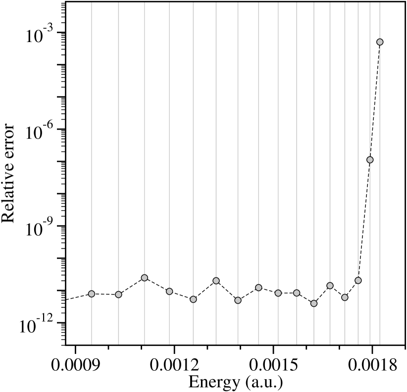
Figure 6: The relative error $|\mathscr{S-\tilde{S}}|/\mathscr{S}$, where $\mathscr{S}$ is the integral on the left-hand-side of Eq. (35) and $\tilde{\mathscr{S}}\equiv|\dot{\tilde{c}}_{\text{res}}|E_{\text{res}}/k_{\text{res}}$ is the right-hand-side. $\mathscr{\tilde{S}}$ was obtained using the value of $\dot{\tilde{c}}$ evaluated as described in Sec. III.3, while $\mathscr{S}=\int\!\phi^{2}$ was computed by numerical quadrature.

For energies within a narrow window centered on $E_{\text{res}}$, we use the approximations

$$a(E) \approx a_{\text{res}}$$

$$c(E) \approx \dot{c}_{\text{res}}(E-E_{\text{res}})$$

$$\phi(E;R) \approx \phi(E_{\text{res}};R).$$

The latter holds for $R$ throughout the inner region and most of the barrier, and thus the probability density inside the inner potential well reads

$$\big{|}\psi(E;R)\big{|}^{2}\approx\frac{a_{\text{res}}}{1+\dot{c}^{2}_{\text{res}}(E-E_{\text{res}})^{2}}\phi^{2}_{\text{res}}(R),$$

where $\phi_{\text{res}}(R)\equiv\phi(E_{\text{res}};R)$. We now substitute $|\dot{c}_{\text{res}}|=\frac{2}{\Gamma}$ from Eq. (31) and make use of the scaling (19) to recast the expression above such that the familiar Breit–Wigner expression, i.e., the Lorentzian energy dependence sharply peaked at $E=E_{\text{res}}$, is made explicit for the wave function itself,

$$\big{|}\psi(E;R)\big{|}^{2}\approx\frac{\frac{\Gamma}{2}}{\big{(}E-E_{\text{res}}\big{)}^{2}+\left(\frac{\Gamma}{2}\right)^{2}}\big{|}\dot{\tilde{c}}_{\text{res}}\big{|}^{-1}\phi^{2}_{\text{res}}(R).$$

For $E=E_{\text{res}}$ the equation above reads

$$\big{|}\psi_{\text{res}}(R)\big{|}^{2}\approx\frac{2}{\Gamma}\big{|}\dot{\tilde{c}}_{\text{res}}\big{|}^{-1}\phi^{2}_{\text{res}}(R),$$

which we now use to rewrite Eq. (33),

$$\int_{0}^{R_{\rm out}}\!\!\!\phi^{2}_{\rm res}(R)\,dR\approx\big{|}\dot{\tilde{c}}_{\text{res}}\big{|}\frac{E_{\rm res}}{k_{\rm res}}.$$ (35)

We emphasize that the approximations used above, as well as in deriving the Breit–Wigner result (33), are excellent for ultra-narrow resonances. Indeed, Fig. 6 shows that Eq. (35) is valid to high accuracy for the resonances located deep below the top of the barrier, which demonstrates that our numerical approach can reach a high level of precision. The approximate nature of Eq. (35) is only visible for the highest two resonances located just under the top of the barrier. Finally, we remark that although Eq. (33) yields essentially exact results for the widths of ultra-narrow resonances, the resonantly enhanced amplitude of $\psi_{\text{res}}(R)$ at short range cannot be pinned down by scanning the energy directly when $\Gamma\lll E_{\text{res}}$ (see discussion at the end of Sec. IV.1). Nevertheless, even if the phase-amplitude approach is not employed, it does suggest a simple remedy for finding the correct physical wave function $\psi_{\text{res}}$ when solving the radial equation (1) directly; namely, the resonance position $E_{\text{res}}$ is first found, and subsequently the (unknown) phase shift $\delta$ is varied instead of the energy (which is kept fixed). Thus, for $E=E_{\text{res}}$, the solution $\psi_{E}$ is initialized asymptotically using $\psi_{E}(\delta;R)=\cos(\delta)j_{\ell}(kR)+\sin(\delta)n_{\ell}(kR)\approx\sin(kR-\ell\frac{\pi}{2}+\delta)$, and is propagated inward. The phase shift $\delta$ is then adjusted to maximize the short-range amplitude of $\psi_{E}(\delta;R)$.

V Summary and outlook

The appeal of Milne’s phase-amplitude representation Milne (1930) stems from the fact that it only requires the computation of slowly varying phase and amplitude functions instead of highly oscillatory wave functions. However, this advantage cannot be fully exploited unless special algorithms are devised for honing in on the smooth solution. For scattering problems, an efficient method was developed by the present authors Shu et al. (2018) for computing the smooth amplitude in the asymptotic region. On the other hand, for classically allowed regions of finite extent, an optimization procedure is needed to find the smooth amplitude; we have developed such an optimization algorithm Shu et al. for locally adapted solutions, which we employed in this work.

We recently formulated an integral representation for phase shifts Shu et al. (2018) based on a phase-amplitude approach Milne (1930); however, our computational method was only applicable to the case of a single (infinite) classically allowed region. In order to generalize our previous work Shu et al. (2018), we have now developed a phase-amplitude approach for tackling scattering potentials with a barrier. As shown in this article, our new method is especially useful for energies below the top of the barrier, when two disjoint classically allowed regions exist. In particular, accurate values of resonance widths in the extreme regime of ultra-narrow resonances ($\Gamma\lll E_{\text{res}}$) can be easily obtained. Numerical results are presented for a representative example of an interaction potential. We also perform an accuracy test which shows that our method is robust for very large barriers.

The approach presented here could be adapted to shape resonances in low energy scattering Côté et al. (1999), and to ultra-long-range Rydberg molecular potentials Stanojevic et al. (2006, 2008), and may also prove useful for analyzing threshold behavior Côté et al. (2004, 1996) relevant to ultracold molecules Côté and Dalgarno (1999); Byrd et al. (2010), especially when near-threshold resonances exist Simbotin et al. (2014); Simbotin and Côté (2015); Shu et al. (2016, 2017). Moreover, we are currently investigating the possibility of extending the phase-amplitude formalism to coupled-channel problems which would allow studies of Feshbach resonances Gacesa et al. (2008); Deiglmayr et al. (2009).

Appendix A Proof of the linear independence of the fundamental set of solutions $\{\phi^{2}$, $\chi^{2}$, $\phi\chi\}$

In our previous work Shu et al. (2018) it was shown that if $\phi$ and $\chi$ are any two solutions of the radial Schrödinger equation (1), then $\phi^{2}$, $\chi^{2}$, and $\phi\chi$ are particular solutions of the envelope equation. Here we prove that the triplet $\{\phi^{2},\chi^{2},\phi\chi\}$ is a basis in the three-dimensional space of solutions of Eq. (2), if $\phi$ and $\chi$ are linearly independent; specifically, we show that the linear combination

$$\rho=a\phi^{2}+b\chi^{2}+2c\phi\chi$$ (36)

vanishes if and only if $a=b=c=0$. We first use the fact that any solution of the envelope equation yields an invariant Shu et al. (2018),

$$Q=\frac{1}{2}\rho\rho^{\prime\prime}-U\rho^{2}-\frac{1}{4}(\rho^{\prime})^{2},$$ (37)

and we employ Eq. (36) to substitute $\rho$, $\rho^{\prime}$ and $\rho^{\prime\prime}$ in terms of $\phi$ and $\chi$ in the equation above; a straightforward but tedious manipulation yields

$$Q=(ab-c^{2})W^{2},$$ (38)

where $W$ is the Wronskian of $\phi$ and $\chi$. If $\rho=0$ in Eq. (36), we obtain $Q=0$ trivially from Eq. (37), while the linear independence of $\phi$ and $\chi$ ensures $W\neq 0$, and consequently Eq. (38) yields

$$ab=c^{2}.$$

We now consider the two possible cases: $c=0$ and $c\neq 0$. In the first case we have $c^{2}=ab=0$, which implies $a=0$ or $b=0$; the vanishing of the remaining coefficient ($b$ or $a$, respectively) follows from our assumption, i.e., $\rho=0$ in Eq. (36). For the second case ($c\neq 0$, and hence $ab\neq 0$), we substitute $c=\operatorname{sgn}(c)\sqrt{ab}$ in Eq. (6), and we obtain

$$\rho=\pm\Psi^{2},$$

where $\Psi$ is the linear combination

$$\Psi=\phi\sqrt{|a|}\pm\chi\operatorname{sgn}(c)\sqrt{|b|}.$$

In the two expressions above, the algebraic sign ($\pm$) is $\operatorname{sgn}(a)=\operatorname{sgn}(b)$. Finally, $\rho=0$ in Eq. (36) yields $\Psi=0$, and the equation above implies $a=b=0$, because $\phi$ and $\chi$ are linearly independent. This contradicts the assumption $ab\neq 0$ in the second case, which completes our proof. Thus, Eq. (36) with arbitrary constants $a$, $b$ and $c$ can indeed be regarded as the general solution of the envelope equation.

Appendix B Extending Milne’s phase outside its domain of smoothness

In this appendix we derive a formula for extending the outer phase $\theta$ into the inner region. First, the inward propagation of $\theta$ through the outer region (including the barrier) is accomplished using the numerical method developed in our previous work Shu et al. (2018). Next, we use Eqs. (5) and (6) to obtain $\theta(R)$ inside the inner region ($0<R<R_{\text{in}}$),

$$\theta_{*}-\theta(R)=\int_{R}^{R_{\text{in}}}\!\!\frac{k}{\rho(r)}dr=k\!\!\int_{R}^{R_{\text{in}}}\frac{dr}{a\phi^{2}+b\chi^{2}+2c\phi\chi},$$

where $\theta_{*}\equiv\theta(R_{\text{in}})$ is known. As explained in Sec. II.1, the integral cannot be handled numerically inside the inner region; instead, we tackle it formally. Making use of the Wronskian $W=\phi^{\prime}\chi-\phi\chi^{\prime}\neq 0$, which is independent of $r$, we rewrite the integral above,

$$\theta_{*}-\theta(R)=\frac{k}{W}\!\int_{R}^{R_{\text{in}}}\!\!\frac{\phi^{\prime}\chi-\phi\chi^{\prime}}{a\phi^{2}+b\chi^{2}+2c\phi\chi}dr.$$

Next, we define $z(r)\equiv\frac{\phi(r)}{\chi(r)}$ and we change the integration variable from $r$ to $z$, but we do so only after the inner region is partitioned in sub-intervals delimited by the nodes of $\chi(r)$, such that $z(r)$ is a one-to-one mapping inside each interval. The change of variable yields

$$\theta_{*}-\theta(R) = k\!\int_{R}^{R_{n}}\!\frac{dr}{\rho(r)}+k\!\sum_{j=n}^{N_{*}}\!\int_{R_{j}}^{R_{j+1}}\frac{dr}{\rho(r)}$$ (39)

$$= \frac{k}{W}\left(\int_{z(R)}^{\infty}\frac{dz}{az^{2}+2cz+b}+(N_{*}-n)\int_{-\infty}^{+\infty}\frac{dz}{az^{2}+2cz+b}+\int_{-\infty}^{z_{*}}\frac{dz}{az^{2}+2cz+b}\right),$$

where $R_{1},R_{2},\ldots,R_{N_{*}}$ are the nodes of $\chi$ inside the inner region, while $R_{0}=0$ and $R_{N_{*}+1}=R_{\text{in}}$ are its boundaries. The node $R_{n}>R$ is the node closest to $R$ inside the integration domain $[R,R_{\text{in}}]$. The upper limit of the last integral is $z_{*}\equiv\frac{\phi(R_{\text{in}})}{\chi(R_{\text{in}})}$. The new integration variable $z$ in Eq. (39) makes it clear that, except for the first and last interval, all other ($N_{*}-n$) intervals give identical contributions.

Making use of the constraint (7), the integral appearing repeatedly in Eq. (39) takes a simple form,

$$\frac{k}{W}\int\frac{dz}{az^{2}+2cz+b}=\arctan\left(\frac{W}{k}(az+c)\right),$$

which we now evaluate for each interval. The contribution of the first interval is

$$\frac{k}{W}\int_{z(R)}^{\infty}\frac{dz}{az^{2}+b+2cz}=\frac{\pi}{2}-\arctan\left(\frac{W}{k}[a\,z(R)+c]\right),$$

while the last interval yields

$$\frac{k}{W}\int_{-\infty}^{z_{*}}\frac{dz}{az^{2}+b+2cz}=\arctan\left(\frac{W}{k}(az_{*}+c)\right)+\frac{\pi}{2}.$$

As mentioned above, the ($N_{*}-n$) remaining intervals give identical contributions; namely, for $n\leq j\leq N_{*}-1$, we have

$$k\int_{R_{j}}^{R_{j+1}}\frac{dr}{\rho(r)}=\frac{k}{W}\int_{-\infty}^{+\infty}\frac{dz}{az^{2}+b+2cz}=\pi.$$

Finally, we add the contributions from all intervals to obtain the outer phase $\theta$ inside the inner region,

$$\theta(R) = \arctan\left(\frac{W}{k}[a\,z(R)+c]\right),$$

$$- \arctan\left(\frac{W}{k}(c+az_{*})\right)+\theta_{*}-\pi(N_{*}-n+1).$$

This result is of key importance, as it yields the scattering phase shift; see Sec. II.4.

Appendix C Choosing the location of the matching point

For energies above the barrier, $R_{\text{top}}$ is a convenient location for the matching point, while for scattering energies below the top of the barrier the matching conditions are imposed at $R_{\text{in}}$. However, for $E<E_{\text{top}}$, the matching point can be placed anywhere within the classically forbidden region under the barrier, despite the fact that in Sec. II.3 we argued that the matching point be located at the turning point $R_{\text{in}}$ (see Fig. 1). $R_{\text{in}}$ is a necessary choice for the matching point only if the phase-amplitude approach is restricted to the outer region; see Sec. II.3. Indeed, if the phase-amplitude method is also used in the inner region, the matching point need no longer be kept at (or near) $R_{\text{in}}$. The freedom to relax the location of the matching point stems from the fact that the inner solutions $\phi$ and $\chi$ can be parametrized in terms of the inner envelope $\varrho$ and phase $\beta$, as shown in Sec. II.5. Accordingly, the solutions (14) of the the matching equations (8) are expressed entirely in terms of phase-amplitude quantities and remain highly accurate if the matching point (which we now denote $R_{*}$) is moved between $R_{\text{in}}$ and $R_{\text{out}}$ (the outermost turning point).

Although the scaled coefficients introduced in Eq. (20) are formally independent of the matching point, their simplified expressions (21) are no longer independent of $R_{*}$. To clarify this aspect, we now analyze the $R_{*}$ dependence of the inner-region phase $\beta_{\text{full}}$ in Eq. (22) to show that for energies sufficiently lower than $E_{\text{top}}$ the phase $\beta_{\text{full}}(R_{*})$ is practically independent of the matching point. Specifically, we make use of the definition (15) to evaluate the derivative $\eta^{\prime}=d\eta/dR_{*}$, while from Eq. (12) we have $\beta^{\prime}=q/\varrho$. Taking advantage of the invariant (37) with $Q=q^{2}$ and $Q=k^{2}$ for $\varrho$ and $\rho$, respectively, we obtain

$$\beta^{\prime}_{\text{full}}=\beta^{\prime}+\eta^{\prime}=\frac{k^{2}\varrho}{\rho^{2}q}\sin^{2}\eta,$$

which is vanishingly small for $E$ sufficiently lower than $E_{\text{top}}$. Indeed, if $R_{*}=R_{\text{in}}$, we have $\rho(R_{*})\ggg 1$, which ensures $\beta^{\prime}+\eta^{\prime}\approx 0$. If $R_{*}$ is shifted away from $R_{\text{in}}$, then $\varrho$ increases while $\eta$ and $\rho$ decrease; from Eq. (15) we have $\eta\sim\frac{1}{\varrho}$ when $\varrho\ggg 1$, and we find

$$\beta^{\prime}_{\text{full}}=\beta^{\prime}+\eta^{\prime}\sim\frac{k}{\rho^{2}\varrho}\approx 0.$$

Therefore, we have

$$\beta_{\text{full}}(R_{*})=\beta(R_{*})+\eta(R_{*})\approx\text{constant,}$$

which justifies our interpretation of $\beta+\eta=\beta_{\text{full}}$ as the full phase accumulated at short range, including the contribution from the barrier region; indeed, when $R_{*}$ is near $R_{\text{out}}$, we have $\eta\approx 0$, and thus

$$\beta_{\text{full}}(R_{*})\approx\beta(R_{\text{out}}),\quad\text{for }R_{\text{in}}\leq R_{*}\leq R_{\text{out}}.$$

Finally, we remark that $R_{*}=R_{\text{top}}$ is a convenient choice for the matching point for all energies (below and above the barrier). In general, the matching point can be energy dependent, e.g., the turning point $R_{\text{in}}(E)$. Therefore, in order to ensure the quantities $\beta$, $\eta$, $u$ and $\varepsilon$ introduced in Sec. II.5 have a well defined energy dependence, the matching point $R_{*}(E)$ must be chosen such that it is a well behaved function of energy.

References

- Shu et al. (2018) D. Shu, I. Simbotin, and R. Côté, Phys. Rev. A 97, 022701 (2018).
- Milne (1930) W. E. Milne, Phys. Rev. 35, 863 (1930).
- Hazi and Taylor (1970) A. U. Hazi and H. S. Taylor, Phys. Rev. A 1, 1109 (1970).
- Mandelshtam et al. (1993) V. A. Mandelshtam, T. R. Ravuri, and H. S. Taylor, Phys. Rev. Lett. 70, 1932 (1993).
- Babb and Du (1990) J. F. Babb and M. L. Du, Chem. Phys. Lett. 167, 273 (1990).
- Sidky and Ben-Itzhak (1999) E. Y. Sidky and I. Ben-Itzhak, Phys. Rev. A 60, 3586 (1999).
- Gibson et al. (1998) G. N. Gibson, G. Dunne, and K. J. Bergquist, Phys. Rev. Lett. 81, 2663 (1998).
- Mrugała (2008) F. Mrugała, J. Chem. Phys. 129, 064314 (2008).
- Greene et al. (1982) C. H. Greene, A. R. P. Rau, and U. Fano, Phys. Rev. A 26, 2441 (1982).
- Yoo and Greene (1986) B. Yoo and C. H. Greene, Phys. Rev. A 34, 1635 (1986).
- Robicheaux et al. (1987) F. Robicheaux, U. Fano, M. Cavagnero, and D. A. Harmin, Phys. Rev. A 35, 3619 (1987).
- Raoult and Balint-Kurti (1988) M. Raoult and G. G. Balint-Kurti, Phys. Rev. Lett. 61, 2538 (1988).
- Fourré and Raoult (1994) I. Fourré and M. Raoult, J. Chem. Phys. 101, 8709 (1994).
- Bohn (1994) J. L. Bohn, Phys. Rev. A 49, 3761 (1994).
- Burke et al. (1998) J. P. Burke, C. H. Greene, and J. L. Bohn, Phys. Rev. Lett. 81, 3355 (1998).
- Bohn and Julienne (1999) J. L. Bohn and P. S. Julienne, Phys. Rev. A 60, 414 (1999).
- Ch. Jungen and Texier (2000) Ch. Jungen and F. Texier, J. Phys. B 33, 2495 (2000).
- Bar-Shalom et al. (2001) A. Bar-Shalom, M. Klapisch, and J. Oreg, J. Quant. Spectr. Rad. Transf. 71, 169 (2001).
- Crubellier and Luc-Koenig (2006) A. Crubellier and E. Luc-Koenig, J. Phys. B 39, 1417 (2006).
- Lecomte and Raoult (2007) J. M. Lecomte and M. Raoult, Mol. Phys. 105, 1575 (2007).
- Zhao et al. (2012) L. B. Zhao, I. I. Fabrikant, J. B. Delos, F. Lépine, S. Cohen, and C. Bordas, Phys. Rev. A 85, 053421 (2012).
- Hall et al. (2013) F. H. J. Hall, M. Aymar, M. Raoult, O. Dulieu, and S. Willitsch, Mol. Phys. 111, 1683 (2013).
- Price and Greene (2018) T. J. Price and C. H. Greene, J. Phys. Chem. A 122, 8565 (2018).
- Kiyokawa (2015) S. Kiyokawa, AIP Adv. 5, 087150 (2015).
- Cariglia et al. (2018) M. Cariglia, A. Galajinsky, G. W. Gibbons, and P. A. Horvathy, Eur. Phys. J. C 78, 314 (2018).
- (26) J. E. Lidsey, arXiv:1802.09186 .
- Schief (1997) W. K. Schief, Appl. Math. Lett. 10, 13 (1997).
- Moyo and Leach (2000) S. Moyo and P. G. L. Leach, J. Math. Anal. Appl. 252, 840 (2000).
- Pinney (1950) E. Pinney, Proc. Am. Math. Soc. 1, 681 (1950).
- Eliezer and Gray (1976) C. Eliezer and A. Gray, SIAM J. Appl. Math. 30, 463 (1976).
- Reid and Ray (1980) J. L. Reid and J. R. Ray, J. Math. Phys. 21, 1583 (1980).
- Korsch and Laurent (1981) H. J. Korsch and H. Laurent, J. Phys. B 14, 4213 (1981).
- (33) D. Shu, I. Simbotin, and R. Côté, arXiv:1612.07849 .
- Maitra and Heller (1996) N. T. Maitra and E. J. Heller, Phys. Rev. A 54, 4763 (1996).
- Côté et al. (1997) R. Côté, H. Friedrich, and J. Trost, Phys. Rev. A 56, 1781 (1997).
- Segev et al. (1997) B. Segev, R. Côté, and M. G. Raizen, Phys. Rev. A 56, R3350 (1997).
- Côté et al. (1998) R. Côté, B. Segev, and M. G. Raizen, Phys. Rev. A 58, 3999 (1998).
- Breit and Wigner (1936) G. Breit and E. Wigner, Phys. Rev. 49, 519 (1936).
- Allison (1969) A. C. Allison, Chem. Phys. Lett. 3, 371 (1969).
- Jackson and Wyatt (1970) J. L. Jackson and R. E. Wyatt, Chem. Phys. Lett. 4, 643 (1970).
- Sando and Dalgarno (1971) K. M. Sando and A. Dalgarno, Mol. Phys. 20, 103 (1971).
- Newton (1982) R. G. Newton, Scattering Theory of Waves and Particles, 2nd ed. (Springer-Verlag, New York, 1982).
- Taylor (1972) J. R. Taylor, Scattering Theory (Wiley, New York, 1972).
- Côté et al. (1999) R. Côté, A. Dalgarno, A. M. Lyyra, and L. Li, Phys. Rev. A 60, 2063 (1999).
- Stanojevic et al. (2006) J. Stanojevic, R. Côté, D. Tong, S. M. Farooqi, E. E. Eyler, and P. L. Gould, Eur. Phys. J. D 40, 3 (2006).
- Stanojevic et al. (2008) J. Stanojevic, R. Côté, D. Tong, E. E. Eyler, and P. L. Gould, Phys. Rev. A 78, 052709 (2008).
- Côté et al. (2004) R. Côté, E. I. Dashevskaya, E. E. Nikitin, and J. Troe, Phys. Rev. A 69, 012704 (2004).
- Côté et al. (1996) R. Côté, E. J. Heller, and A. Dalgarno, Phys. Rev. A 53, 234 (1996).
- Côté and Dalgarno (1999) R. Côté and A. Dalgarno, J. Mol. Spectrosc. 195, 236 (1999).
- Byrd et al. (2010) J. N. Byrd, J. A. Montgomery, Jr., and R. Côté, Phys. Rev. A 82, 010502 (2010).
- Simbotin et al. (2014) I. Simbotin, S. Ghosal, and R. Côté, Phys. Rev. A 89, 040701 (2014).
- Simbotin and Côté (2015) I. Simbotin and R. Côté, Chem. Phys. 462, 79 (2015).
- Shu et al. (2016) D. Shu, I. Simbotin, and R. Côté, Chem. Phys. Chem. 17, 3655 (2016).
- Shu et al. (2017) D. Shu, I. Simbotin, and R. Côté, J. Phys. B 50, 204003 (2017).
- Gacesa et al. (2008) M. Gacesa, P. Pellegrini, and R. Côté, Phys. Rev. A 78, 010701 (2008).
- Deiglmayr et al. (2009) J. Deiglmayr, P. Pellegrini, A. Grochola, M. Repp, R. Côté, O. Dulieu, R. Wester, and M. Weidemüller, New J. Phys. 11, 055034 (2009).